WHAT DRIVES THE VIX AND THE VOLATILITY RISK PREMIUM?∗

Elena Andreou† Eric Ghysels‡

First Draft: February 2012

This Draft: September 29, 2013PRELIMINARY AND INCOMPLETE

Abstract

There is a long tradition in finance of characterizing compensation for risk as a linear function of factors. The most

common examples are linear models for equity risk premia, such as the CAPM and APT pricing models. We develop

an econometric methodology to infer factors from a large panels of (filtered) volatilities. The panels are not confined

to equity volatilities, but cover a wide range of financial instruments. Motivated by affine jump diffusion no-arbitrage

asset pricing models, we present a formal framework for factor estimation with panels consisting of various filtered

volatilities, either ARCH-type or realized. The theoretical pricing formulas combined with the asymptotic properties

of the filtering procedures allows us to invoke large factor model asymptotic theory to obtain factor estimates. Using

a large panel of financial instruments related to corporate credit risk, default risk and commodities we extracted

factors and show how they predict the VIX and determine the volatility risk premium.

∗The second author benefited from funding from a Marie Curie FP7-PEOPLE-2010-IIF grant. We thank Ron Gallant, LarsHansen, Jonathan Hill, Adam McCloskey, Serena Ng and Eric Renault for some helpful comments while writing the paper.†Department of Economics, University of Cyprus, P.O. Box 537, CY 1678 Nicosia, Cyprus, e-mail:

elena.andreou@ucy.ac.cy.‡Department of Economics, University of North Carolina, Gardner Hall CB 3305, Chapel Hill, NC 27599-3305, USA, and

Department of Finance, Kenan-Flagler Business School, e-mail: eghysels@unc.edu.

1 Introduction

There is a long tradition in finance to characterize compensation for risk as determined by a linear functionof factors. This is true for stock market valuation, where, for example, the widely used Fama-French three-factor model can be interpreted in the framework of the no-arbitrage theory of Ross (1976b), in yield curveand credit risk modeling, where models by Vasicek (1977), Duffie and Kan (1996), and Dai and Singleton(2000) are typical examples, as well as derivatives pricing (i.e., Heston (1993), Bates (1996), Duffie, Pan,and Singleton (2000)).

This paper is related to the extant literature in a number of ways. The extraction of risk factors is typicallyconfined to a particular asset class. Fama-French factors are extracted from cross-sections of stock returnsand are meant to price equity risk. Level, slope and curvature factors are extracted from fixed incomesecurities and meant to price the term structure. Default risk is extracted from panels of corporate bondsand meant to assess such risk across a wide spectrum of credit quality, etc. A few attempts have been madeto price across asset classes, see Bakshi and Chen (1997), Bekaert and Grenadier (1999), Bakshi and Chen(2005), Bekaert, Engstrom, and Xing (2009), Bekaert, Engstrom, and Grenadier (2010), Koijen, Lustig, andVan Nieuwerburgh (2010), Lettau and Wachter (2011), among others, use the class of affine asset pricingmodels to extract factors jointly from stocks and bonds. Our paper proposes new ways to extract risk factors,and suggests how to use a broad class of assets ranging from equities, sovereign and corporate bonds, shortterm lending, commodities and foreign exchange, to do so.

While our primary focus is on volatility risk factors, in particular those related to the VIX, we find suchfactors are also useful in predicting future equity returns. Regarding the extraction of volatility risk factors,we propose a novel approach. In particular, we extract such factors from panels of filtered volatilities usingARCH-type models. We know for sure that ARCH models are the wrong models, yet as argued by Nelson(1990), Nelson and Foster (1994), Nelson (1996), among others, they can be viewed as filters and deliverreliable estimates of spot volatility despite their mis-specification. To obtain such results we need somecontinuous record asymptotic arguments about the samples used to estimate the volatilities. On top of this,we need both large cross-sections (of dimension N) of such volatilities and we need a reasonably long timeseries (of length T). This entails some challenges regarding the large sample analysis used to estimate thevolatility risk factors. In a companion theory paper (Andreou and Ghysels (2013)) the authors show that,contrary to the root-N standard normal consistency, one finds N -consistency, also standard normal, due tothe fact that the high frequency sampling scheme is tied to the size of the cross-section, boosting the rate ofconvergence. We apply this new estimation strategy to new panel data sets of filtered volatilities, to uncoverthe driving factor for the VIX and volatility risk premium.

A number of papers have considered extracting factors using a classical factor analysis using (finitedimensional) panels of option-based implied volatilities - see e.g. Carr and Wu (2009), Egloff, Leippold,and Wu (2010), Zhou (2010), Bakshi, Panayotov, and Skoulakis (2011), among others. The advantage of

1

our approach is that we use a much broader class of volatilities (and therefore large dimensional), as we arenot limited to (liquid) option-based implied volatilities. Moreover, because of the richness of our panel interms of coverage of different asset classes, including equities, commodities, corporate bonds and FX, wecan identify factors by using only a specific asset class. More specifically, we can extract factors only fromequities, or only from commodities, and use them to put labels on the sources of risk. Note also, that ouranalysis is largely data-driven, namely, simple GARCH models function as filters (the GARCH parameterestimates are not of any direct interest), and principal component analysis is applied to ever expandingcross-sections of time series using high frequency data to generate the panel data of estimated volatilities.

Obviously not all risk factors may be revealed by volatilities, despite the potentially large selection of cross-sectional observations. Therefore, we do not exclusively rely on panels of volatilities. Namely, we alsoconsider panels of a broad class of assets, including commodity returns, credit risk spreads (as well as theirvolatilities), etc. Extracting risk factors from such data does not pose any new technical challenges - unlikethe case of volatilities. Yet, the application goes beyond the traditional factor analysis.

As noted earlier, we use our analysis setup to extract fundamental asset pricing factors and revisit modelingthe economic sources of the VIX and the volatility risk premium (VRP). Is it really the case that a singlefactor drives VRP, or are there multiple factors involved? The single factor argument has been usedextensively in a number of recent papers, including Zhou (2010), Mueller, Vedolin, and Zhou (2011)and Wang, Zhou, and Zhou (2013), among others, to argue that the VRP predicts risk premia acrossequity, bond, currency, and credit markets. These findings are inspired by the Drechsler and Yaron (2011)general equilibrium model that incorporates consumption growth volatility uncertainty and recursive utilitypreferences of a representative agent. Empirically, the volatility of the volatility of consumption growth ishard to pin down, however, and therefore the model implied linear mapping between the so called vol of voland VRP is exploited in empirical analysis. There is reason to believe, however, that a single factor modelmay not be an adequate. Indeed, several recent empirical studies suggest this is the case, including Carrand Wu (2009), Egloff, Leippold, and Wu (2010), Bakshi, Panayotov, and Skoulakis (2011), Christiansen,Schmeling, and Schrimpf (2012), Corradi, Distaso, and Mele (2013) and Engle, Ghysels, and Sohn (2013),among others. The empirical work in our paper is most closely related to recent work by Christiansen,Schmeling, and Schrimpf (2012), Corradi, Distaso, and Mele (2013) and Engle, Ghysels, and Sohn (2013).Corradi, Distaso, and Mele (2013) develop a no-arbitrage affine asset pricing model where stock marketvolatility is explicitly related to a number of macroeconomic and unobservable factors. The model is fullyparameterized and involves two observable factors - inflation and industrial production growth - and anadditional latent third orthogonal factor. While the theoretical framework is powerful and elegant with stockvolatility linked to the factors by no-arbitrage restrictions, it is potentially prone to specification errors. Forexample, Corradi, Distaso, and Mele (2013) assume that inflation and industrial production (IP) growthare driven by two orthogonal factors described by univariate square root processes. In reality inflationand IP growth are not orthogonal, a specification error which affects the parameterization and impliedarbitrage restrictions in the model. Moreover, Christiansen, Schmeling, and Schrimpf (2012) document that

2

purely macroeconomic variables (as opposed to financial variables) hardly show up as important predictorsof financial volatility. Along similar lines, Engle, Ghysels, and Sohn (2013) show that (the long termcomponent) of volatility is not only driven by inflation and industrial production (IP) growth, but also byinflation and IP volatility. In addition, Christiansen, Schmeling, and Schrimpf (2012) find that defaultspreads stand out as useful predictors not only for equity market volatility but also for other asset classes,whereas measures of funding market (il)liquidity and heightened counter-party credit risk also matter forseveral asset classes.

INCOMPLETE

2 Affine Asset Pricing Models

We start with the widely used class of continuous time affine jump diffusion (henceforth AJD) asset pricingmodels. To fix notation, we follow the presentation of Duffie, Pan, and Singleton (2000) and considera filtered probability space (Ω,F , (Ft)t≥0,P) where the filtration satisfies the usual conditions (see e.g.Protter (2004)) and P refers to the physical or historical probably measure. Moreover, we suppose that thek-dimensional F-adapted process X f of state variables or factors is Markov in some state space D ⊂ Rk,

solving the stochastic differential equation:

dX ft = µP(X ft )dt+ σ(X ft )dW Pt (2.1)

where W Pt is an Ft-adapted Brownian motion under P in Rk, µP : D→ Rk, σ : D→ Rk×k. The empirical

analysis in the paper involves asset classes which do not feature reliable intra-daily data, which precludesus from using realized variances using high frequency data. As a consequence, our analysis focuses on theestimation of ARCH-type models, which excludes the presence of jumps. In a richer data environment, wecould easily extend the setting to one including affine jump diffusion processes, see Andreou and Ghysels(2013) for further details. Formally, the affine diffusions satisfy the following:

Assumption 2.1. The distribution of X f , given an initial known X f0 at t = 0, is completely characterizedby the pair (KP, H) of parameters determining the affine functions:

µP(x) = KP0 +KP

1 x, KP ≡ (KP0 ,K

P1 ) ∈ Rk × Rk×k

(σ(x)σ(x)T)ij = (H0)ij + (H1)Tijx H ≡ (H0, H1) ∈ Rk×k × Rk×k×k (2.2)

Finally, we also assume absence of arbitrage, which implies the existence of (Ω,F , (Ft)t≥0,Q) where Q isan equivalent martingale measure under the risk neutral world. Furthermore, we assume that X f is also anaffine diffusion under Q, and therefore:

3

Assumption 2.2. Under the risk-neutral equivalent martingale measure Q the process X is described by:

dX ft = µQ(X ft )dt+ σ(X ft )dWQt (2.3)

completely characterized by the pair (KQ, H, lQ) of parameters determining the affine functions:

µQ(x) = KQ0 +KQ

1 x, KQ ≡ (KQ0 ,K

Q1 ) ∈ Rk × Rk×k

(σ(x)σ(x)T)ij = (H0)ij + (H1)Tijx H ≡ (H0, H1) ∈ Rk×k × Rk×k×k (2.4)

In a generic affine diffusion no-arbitrage asset price setting, Duffie, Pan, and Singleton (2000) show thatthe bond, equity and variance premia at different investment horizons are linear functions of the same riskfactors - i.e. state variables X ft . In the term structure literature it is common to rotate the factors such thatthey correspond to the commonly used level, slope and curvature factors. The equity premia literature hasinstead focused on factors driven by macroeconomic fundamentals, in particular consumption uncertainty inthe context of long-run risk economies studied by Bansal and Yaron (2004), where agents have a preferencefor early resolution of uncertainty and therefore dislike increases in economic uncertainty.1

While we will consider a broad asset class, we start with equity returns. We start with a reduced form forexpected excess log returns (on the market portfolio):

EPt [rt,t+τ ] = γer(τ)X ft , (2.5)

Following Britten-Jones and Neuberger (2000), Jiang and Tian (2005), and Carr and Wu (2009), we definethe variance risk premium (VRP) as the difference between expected variance under the risk-neutral measureand expected variance under the objective measure.

The VRP has been studied extensively as it relates to variance swap contracts for which there is an activemarket particularly pertaining to the S&P 500 stock market index. One leg of the swap will pay an amountbased upon the realized variance of the price changes of the underlying. Conventionally, these price changeswill be daily log returns. The other leg of the swap will pay a fixed amount, which is the strike, quoted at thedeal’s inception. Thus the net payoff to the counter-parties will be the difference between these two and willbe settled in cash at the expiration. Hence, at maturity, the payoff to the long side of the swap is equal to thedifference between the realized variance over the life of the contract and a constant called the variance swaprate. No arbitrage dictates that the variance swap rate equals the risk-neutral expected value of the realizedvariance, i.e. EQ

t [V rt,t+τ ], V r

t,t+τ is the equity return forward integrated variance over the time interval t to t+ τ. The VRP is the difference between the time t expected equity returns variance under the historical (P)and the risk-neutral (Q) probability measures, over horizon τ can be written as:

V RP (t, τ) = EQt [V r

t,t+τ ]− EPt [V r

t,t+τ ] (2.6)1See in particular Eraker and Shaliastovich (2008) for the linear pricing characterization of long-run risk equilibrium models.

4

With the linear affine risk premia setting, one obtains respectively:

V RP (t, τ) = δvrp(τ) + γvrp(τ)X ft , (2.7)

where δvrp and γvrp relate to the data generating process, i.e. relate to αi and βi for i = Q and P (seefor example Todorov (2010), among others, for further details). Similarly, the pricing of future integratedvolatility can be written as:

EQt [V r

t,t+τ ] = µQrv(τ) + γQ

rv(τ)X ft , EPt [V r

t,t+τ ] = µPrv(τ) + γP

rv(τ)X ft (2.8)

The above linear pricing schemes have been used extensively, although with assumed factor representations- and their interpretation - that are different. See notably Carr and Wu (2009), Egloff, Leippold, and Wu(2010), Zhou (2010), Bakshi, Panayotov, and Skoulakis (2011), Mueller, Vedolin, and Zhou (2011), Wang,Zhou, and Zhou (2013) and Corradi, Distaso, and Mele (2013), among others. In the next section, we presenta novel approach of estimating X ft .

By analogy with the term structure of interest rates, one can estimate the principal components for a panelof variance risk premia with different maturities. Buhler (2006), Amengual (2009), Egloff, Leippold, andWu (2010) and Aıt-Sahalia, Karaman, and Mancini (2012) apply principal component analysis (PCA) topanels of variance swap rates and find that two factors - which can be interpreted as level and slope - explainclose to 100 % of the variation in variance swap rates for the S&P 500. The similarities with term structureof interest rates also brings us to the topic of stochastic singularity - since we have potentially large cross-sections of variance swap rates driven - according to equation (2.7 - by just a few state variables. Addingmeasurement errors to the variance swap rates is the standard solution. The analysis in the next section willnot require us to add an ad hoc measurement error as filtered volatilities have a natural error distributionwhich we know how to characterize asymptotically.2

In the empirical section we use five homogeneous classes of assets. Risk pricing for each asset class islinearly affine inX f .Most importantly, however, the different asset classes will - via differences in exposure- give us different snapshots of factor space which spans risk in an unified affine asset pricing world. Forconvenience of presentation we conclude this section with a generic affine pricing formula indexed by anindicator defined for a set of asset classes ranging from equities (already discussed), sovereign and corporatebonds, short term lending, commodities and foreign exchange. We will also need to distinguish ’spread’factors from ’volatility’ factors. The former pertain to respectively default, credit and maturity spreads,whereas the latter will pertain to their volatility, i.e. the volatility of default, credit and maturity spreads.

2Todorov (2010), Bollerslev and Todorov (2011), Aıt-Sahalia, Karaman, and Mancini (2012) find that a large and time-varyingjump risk component is embedded in variance swap rates. Regularity conditions underlying some of the factor filters discussed inthe next section will exclude jump risk, the reason why we need the rely on the more restrictive Assumption 2.1.

5

The distinction is reminiscent of the excess equity returns and their volatility

EPt [ct,t+τ ] = µP

c (τ) + γPc (τ)X ft , EP

t [V ct,t+τ ] = µP

cv(τ) + γPcv(τ)X ft

EQt [ct,t+τ ] = µQ

c (τ) + γQc (τ)X ft , EQ

t [V ct,t+τ ] = µQ

cv(τ) + γQcv(τ)X ft

(2.9)

Before we do, it is worth noting that we do not impose no-arbitrage conditions across pricing equations -unlike for instance Corradi, Distaso, and Mele (2013). Imposing such conditions is a much debated topic inthe term structure of interest literature (see e.g. Duffee (2011)) and as we noted in the Introduction may beprone to mis-specification issues. We therefore do not follow this route. Alternatively, and again similar tothe term structure literature, one might think of backing out factors, using a sufficient number of financialassets - an approach pursued by Carr and Wu (2009), Zhou (2010), Bakshi, Panayotov, and Skoulakis (2011),among others. We will not pursue this approach either.

3 Factor Analysis with Panels of ARCH Filters

The idea to extract factors that determine risk premia has a long tradition both in the equity pricing (Merton(1973), Ross (1976a), Chamberlain and Rothschild (1983), among many others) and fixed income termstructure (Fama and Bliss (1987), Campbell and Shiller (1991), Cochrane and Piazzesi (2005), among manyothers). The method we adopt relates to efforts by Ludvigson and Ng (2009) to find a direct relation betweenbond risk premia and the macro economy. However, we use their techniques in a novel way to extractcommon factors from a large panel of asset volatilities.

Technically speaking we will consider for any asset i with (log) price xit which has exposure to (some of)the risk factors, i.e.:

xit ≡ δi0 + δiX ft δi 6= 0 (3.1)

such as for example the log price of an equity claim, log price of a zero-coupon bond, a risk spread, etc.,and we are interested in two objects: (1) spot volatility and (2) integrated volatility. More precisely, we canwrite spot volatility, simplifying the notation, as:

V it = µP

iv(0) + γPiv(0)X ft ≡ µiv + γivX ft (3.2)

whereas the time t expectation of integrated volatility over horizon τ, namely EPt [V i

t,t+τ ] = µPiv(τ) +

γPiv(τ)X ft , will be studied in the next section. We do not directly observe volatility, integrated or spot,

(nor X ft ) but have at our disposable, for a large set of assets, some estimates for either type of volatility. Wewill start with the spot volatility case and consider integrated volatilities in the next section. We are workingunder the assumption that we can collect volatility data which span the space all the risk factors, formally

6

defined later. Alternatively, we can think of estimating a sub-block of factors pertaining to volatility, whichwe still will denote by X ft to avoid further complicating notation.

Combining equation equations (2.1) and (3.3) implies that xit satisfies the diffusion:

dxit = µi(X ft )dt+ σi(X ft )dW Pt (3.3)

where X ft satisfies Assumption 2.1, and therefore by Ito’s lemma: µi(X ft ) ≡ δiµP(X ft ) and σi(X ft ) ≡σ(X ft ).

When spot volatility is latent it is necessary to think about filtering. There are an abundant number of filteringschemes, many based on Markov Chain Monte Carlo simulation algorithms, inspired by the seminal workof Jacquier, Polson, and Rossi (2002). Such filtering schemes are analytically intractable and unattractivewhen we are dealing with potentially large cross-sections, like hundreds of individual asset volatilities. Wetherefore need to rely on computationally simple filters, convenient and analytically tractable. We thereforeopt for ARCH-type models as filters, following the work of Nelson (1990), Nelson and Foster (1994), Nelson(1996), among others. Hence, we will rely on easy to estimate (univariate) ARCH-type models viewed as afilters through which one passes the data to produce an estimate of the conditional variance.

We lack continuous time observations xit for asset i but have observations, denoted by x[h]ikh with k integer,at arbitrary small time intervals equally spaced by hi and such data can be collected at an ever increasingfrequency, hi ↓ 0 ∀ i. Suppose we denote the filtered volatility by V [h]it and we define:

V [h]it ≡ V it + ε[h]it = µiv + γivX ft + ε[h]it (3.4)

where ε[h]it is a filtering error, i.e. the difference between the true spot volatility and the one obtained fromthe ARCH-filter. Nelson and Foster (1994) use continuous record asymptotics, i.e. using asset log assetprice data at arbitrary small time intervals, denoted by x[h]it for asset i in the cross-section, to characterizethe distribution of the measurement error.

The data structure we have in mind involves three types of asymptotics. There is the cross-section ofvolatilities estimates at each point in time, namely i = 1, . . . , N observed at dates t = 1, . . . , T. Thissetup is reminiscent of the large N and large T asymptotics for panel data models of Stock and Watson(2002), Bai and Ng (2002), Bai (2003), among others. In addition to the expanding N and T, we also havethe sampling frequency h of data used to compute the volatility estimates using data collected at increasingfrequency, h ↓ 0, where h ≡ supi=1,N hi. The sampling scheme we therefore have in mind appears in thefollowing diagram:

7

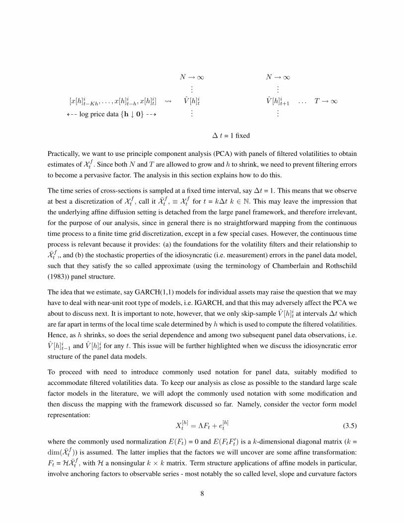
N →∞ N →∞...

...[x[h]it−Kh, . . . , x[h]it−h, x[h]it] V [h]it V [h]it+1 . . . T →∞

L99 log price data h ↓ 0 99K...

...

∆ t = 1 fixed

Practically, we want to use principle component analysis (PCA) with panels of filtered volatilities to obtainestimates of X ft . Since bothN and T are allowed to grow and h to shrink, we need to prevent filtering errorsto become a pervasive factor. The analysis in this section explains how to do this.

The time series of cross-sections is sampled at a fixed time interval, say ∆t = 1. This means that we observeat best a discretization of X ft , call it X ft , ≡ X

ft for t = k∆t k ∈ N. This may leave the impression that

the underlying affine diffusion setting is detached from the large panel framework, and therefore irrelevant,for the purpose of our analysis, since in general there is no straightforward mapping from the continuoustime process to a finite time grid discretization, except in a few special cases. However, the continuous timeprocess is relevant because it provides: (a) the foundations for the volatility filters and their relationship toX ft ,, and (b) the stochastic properties of the idiosyncratic (i.e. measurement) errors in the panel data model,such that they satisfy the so called approximate (using the terminology of Chamberlain and Rothschild(1983)) panel structure.

The idea that we estimate, say GARCH(1,1) models for individual assets may raise the question that we mayhave to deal with near-unit root type of models, i.e. IGARCH, and that this may adversely affect the PCA weabout to discuss next. It is important to note, however, that we only skip-sample V [h]it at intervals ∆t whichare far apart in terms of the local time scale determined by hwhich is used to compute the filtered volatilities.Hence, as h shrinks, so does the serial dependence and among two subsequent panel data observations, i.e.V [h]it−1 and V [h]it for any t. This issue will be further highlighted when we discuss the idiosyncratic errorstructure of the panel data models.

To proceed with need to introduce commonly used notation for panel data, suitably modified toaccommodate filtered volatilities data. To keep our analysis as close as possible to the standard large scalefactor models in the literature, we will adopt the commonly used notation with some modification andthen discuss the mapping with the framework discussed so far. Namely, consider the vector form modelrepresentation:

X[h]t = ΛFt + e

[h]t (3.5)

where the commonly used normalization E(Ft) = 0 and E(FtF ′t) is a k-dimensional diagonal matrix (k =dim(X ft )) is assumed. The latter implies that the factors we will uncover are some affine transformation:Ft = HX ft , with H a nonsingular k × k matrix. Term structure applications of affine models in particular,involve anchoring factors to observable series - most notably the so called level, slope and curvature factors

8

(see e.g. Dai and Singleton (2000) for a detailed discussion). In our analysis, there is no obvious way tocalibrate the level and scale of Ft, and therefore we use a standard normalization. Moreover, we let (a) X [h]

t

= ((V [h]it − v[h]iT ), i = 1, . . . , N)′, where v[h]iT are the sample means for each volatility filter series inthe cross-section - the demeaning absorbs the term µiv + γivE[X ft ], in equation (3.4) since the factors andidiosyncratic errors are mean zero, (b) the factor loadings Λ = (λ1, . . . , λN )′ are non-random and, (c) e[h]

t =(ε[h]it, i = 1, . . . , N)′. The matrix representation of the factor model is:

X [h] = FΛ′ + e[h] (3.6)

where X [h] = (X ′1, . . . , X′N ) is a T × N matrix of observations on demeaned volatilities and e[h] =

((e[h]1 )′, . . . , (e[h]

N )′) a T ×N matrix of idiosyncratic errors. Henceforth, to simplify notation we will denotethe individual elements of X [h] as x[h]

it , and those of e[h] as e[h]it .

The estimator we consider is standard, namely the method of asymptotic principal components, initiated bywas first considered by Connor and Korajczyk ((1986) and (1988)) and refined by Stock and Watson (2002),Bai and Ng (2002), Bai (2003), as an estimator of the factors in a large N and T setup. For any given rnot necessarily equal to the true number of factors k, the method of principal components (PC) constructs aT × r matrix of estimated factors and a corresponding N × r matrix of estimated loadings by solving thefollowing optimization problem for a given h :

minΛ,F

1NT

N∑i=1

T∑t=1

(x[h]it − λ

′iFt)

2 (3.7)

subject to the normalization that (Λ′rΛr)/N = Ir and (F ′rFr) being diagonal. The estimated factor matrixF

[h]t is

√T times the eigenvectors corresponding to the r largest eigenvalues of the T ×T matrix X [h]X [h]′ .

Moreover, Λ′ = (F [h]′F [h])−1F [h]′X [h] are the corresponding factor loadings.

Under suitable regularity conditions, Andreou and Ghysels (2013) show that if√N/T → 0, then for each

t :(√N/h1/4)(F [h]

t −HXft ) d→ N(0, V −1QΛtQ′V −1),

We note from the above that the estimation of the factors has a rate of convergence (√N/h1/4) instead of

the standard√N asymptotic results found in Bai and Ng (2002), Bai (2003), among others. The reason for

the difference is the combination of the continuous record asymptotics of Nelson and Foster (1994) and thelarge panel data analysis. In the latter case, standard central limit theorems are assumed for the error processof the panel data model (see e.g. Assumption F of Bai (2003)). In our analysis, the dependence structureof the errors follow directly from the assumed sampling scheme for the ARCH filters. In fact, if we takeas example h = N−2, we simultaneously squeeze the ARCH filtering errors, and therefore the errors of thepanel data. With h = N−2, we actually obtain a rate of converge equal to N, instead of the usual

√N. This

actually implies that ARCH filter panel data models yield super-consistent estimators, borrowing a concept

9

from the unit root literature (e.g. Dickey and Fuller (1981)), for the factor process X ft .

It should finally also be noted that the number of factors can be consistently estimated the number of factorsk by analyzing the statistical properties of the minimand V (k) appearing in equation (3.7) as a function of k,where k is not necessarily the true k. Bai and Ng (2002) showed that the number of factors can be estimatedconsistently by minimizing the following criterion:

IC(k) = log (V (k)) + k

(N + T

NT

)log(

NT

N + T

)

In terms of practical implementation there is an important lesson which emerges from our analysis. Althoughwe will study monthly panels, our GARCH models will be daily and we will pick the last day of the monthin order to construct our panel data set. Such a strategy will enable us to exploit the idea of using higherfrequency data to extract the monthly volatility risk factors.

4 Factors for the VIX and the Volatility Risk Premium

In the previous section we focused exclusively on extracting volatility risk factors. Our empirical analysisdoes not deal exclusively with panel of GARCH volatility filters, it also includes various risk spreads forexample. Hence, we will drop the h index in this section, although in the background, we should keep inmind that higher frequency data is used to implement our empirical analysis. A consequence of the resultsdiscussed in the previous implies that we cannot pool panels of filtered volatilities with other standard paneldata, since the convergence rates differ. We will therefore proceed with estimating factors by asset class andtreat separately the return/spread and volatility panels. For each class we extract return/spread risk factorsand return/spread volatility risk factors. In particular, we extract factors from a panel of homogeneous assetclasses e.g. corporate risk, commodity price risk, which allow us to identify the specific sources of riskassociated with these particular classes of financial assets. Second, we apply the ideas spelled out in theprevious section, by extracting factors from daily GARCH models. Typically factors are extracted from aspecific asset class (e.g. term structure) to price the same type of assets (e.g. fixed income derivatives). Weextract factors of say, short term funding risk, long-run corporate spreads risk, commodity risk and showhow it helps pricing equity volatility risk, the RV of S&P500 stock market returns, the VIX as well as VRP.

4.1 Factor Extraction

We extract common factors for panels that are stratified by asset class (e.g. commodities) and subclasses(e.g. energy and metals commodities). The panel of daily GARCH models sampled end of each monthconsist of (i) energy and metals commodity returns and spreads, (ii) long-run corporate bond spreads and

10

(iii) short-run funding spreads during 1999m01 - 2010m12, T = 144. More specifically:

(i) The short-run funding risk panel (N = 35) are volatilities of e.g. the LIBOR, Eurodollar, (Non)Commercial (Non) Financial paper short-run spreads and Tbills of different maturities (7 Days,1,3,6,12months) with respect the Fed funds rate, summarized by category in Appendix Table A.1 and listed indetail in Appendix Table A.4. For each series an AR(1)-GARCH(1,1) model is estimated as a proxy of thevolatility of each spread. The common volatility factor estimated from the volatility panel is denoted bySRFUN VF. The corresponding factor estimated from the returns panel is SRFUN SF.

(ii) The long-run corporate risk panel (N = 74) involves volatilities of corporate bond spreads fromdifferent industries, indices, maturities, rating categories vis-a-vis the corresponding government bondmaturity (e.g. 1,5,7,10 years) summarized by category in Appendix Table A.2 and listed in detail inAppendix Table A.5. As above an AR(1)-GARCH(1,1) model is estimated for each spread series. Thefirst principal component or factor estimated from this panel of volatilities is denoted by LRCOR VF andthe corresponding one from just the spreads LRCOR SF.

(iii) The energy and metals commodities risk block is based on a homogeneous panel of volatilities ofenergy and metal commodities (N = 122) of various spot and future returns e.g. of gas, oil, biofuel andvarious metals e.g. gold, silver, aluminium e.t.c, as well as corresponding indices described by categoryin Appendix Table A.3, and the corresponding spreads between spot and futures prices of each commodity.The detailed list of the series can be found in Table A.6. For each series we estimate an AR(1)-GARCH(1,1)model. The common volatility factor estimated from the panel of volatilities is denoted by EM VF and thecorresponding one from returns and spreads is denoted by EM RF.

Using the AR(1)-GARCH(1,1) univariate filters in panel (i) above, the short-run funding risk volatility factor(SRFUN VF) explains 65% of the variation of the panel as given by the sum of squared loadings. Thisfactor loads heavily on the following types of spreads: 15Day A2/P2/F2 Nonfinancial Commercial Paper(% Per Annum) -15Day Aa Financial Commercial Paper (% Per Annum), 15Day A2/P2/F2 NonfinancialCommercial Paper (% Per Annum) -15Day Aa Nonfinancial Commercial Paper (% Per Annum) and 7DayLondon Interbank Offered Rate (%) -FF.3 We find that the corresponding SRFUN RV factor explains also81% of the variation of the series in this panel.

In the second panel of the corporate risk we extract the common factor from the AR(1)-GARCH(1,1)univariate filters of long-run corporate spreads which is denoted by LRCOR VF and explains 75% variationof this panel. The LRCOR VF factor explains 85% of the variation of the panel and loads heavilyon the following types of volatility spreads: Merrill Lynch Treasury Master: Effective Yield (%)-10Yr-Tbond, Merrill Lynch Treasury Master: Yield To Worst (%)-10Yr-Tbond, Merrill Lynch Corporate Bonds:Industrials: 1 to 3 Yrs: Effective Yield (%) -3Yr-Tnote and Merrill Lynch Corporate Bonds: Utilities: 1 to

3For robustness we also obtain the corresponding factor from the panel of univariate monthly Realized volatilities based on theaggregated squared residuals of the daily AR(1) of the spreads.

11

3 Yrs: Effective Yield (%) -3Yr-Tnote. Note that the corresponding factor based on the Realized Volatilityof the squared residuals of the daily AR(1) of the spreads, LRCOR RV, also explains 85% of the variationin the panel.

The last panel of the energy and metals commodities returns and spreads volatilities yields a commonvolatility factor which explains 95% of the variation of this panel of asset volatilities and correlates highlywith the volatilities of the following series: S&P GSCI Heating Oil Total Return Index (Dec-31-82=100),No 2 Heating Oil Futures Price: 3-Month Contract Settlement ($/Gal) and S&P GSCI Energy CommoditiesTotal Return Index (12/31/82=100).

We examine the predictive ability of these factors, SRFUN VF, LRCOR VF and EM VF, in explaining theVIX, the Realized Volatility of the S&P 500 (RV SP500) and the VRP at different horizons. The VIX isthe Chicago Board Options Exchange Market Volatility Index, a measure of the implied volatility S&P 500index options. We model the VIX2. The monthly RV measure for the S&P 500 is the summation of the78 within day five-minute squared returns covering the normal trading hours from 9:30am to 4:00pm plusthe close-to-open overnight return. For a typical month with 22 trading days, this leaves us with a total ofT = 22× 78 = 1716 five-minute returns. The variance risk premium is a common short-run component ofthe market risk premia which is not directly observable but an empirical proxy can be constructed from thedifference between model-free option-implied variance (VIX2) and the conditional expectation of model-free realized variance RV SP500.

5 What drives the VIX, RV SP500 and VRP?

In this section we focus the discussion on the results related to the two novel volatility factors, the short-runfunding risk spread volatility factor, SRFUN VF, and the energy and metals volatility factor, EM VF, whichpredict the VIX2, RV SP500 and VRP for alternative forecast horizons, h, and model specifications usingin-sample analysis. A number of additional results are discussed and presented in the robustness section 6.

Table 1 presents the estimated linear predictive regression models for the VIX2 during the period 1999m01- 2010m12 for alternative forecasting horizons of H = 6, 9 and 12 months. The LS parameter estimatesand the Newey West HAC standard errors with fixed bandwidth are reported along with the adjusted R2

for each model. The following models are specified: Models 1 and 2 in Table 1 represent the benchmarkmodels. In model 1 the VIX2 follows a simple AR(H) process and in model 2 the VIX2 is driven by itsown lag and that of the volatility of consumption along the lines of models of Drechsler and Yaron (2011).Note that we proxy the volatility of the volatility of consumption using the AR-GARCH fitted values ofthe monthly per capita consumption on non-durables and services. This series is also used in Drechslerand Yaron (2011) and Bansal and Shaliastovich (2013). Alternative measures of consumption volatility arealso addressed in the robustness section. The corresponding single factor model specification for the VIX2

12

which is closer to the theory e.g. Drechsler and Yaron (2011) is given by model 7 and includes only thevolatility of consumption, DLC V(−H). The remaining models considered in table 1 incorporate our newvolatility factors , EM VF(−H) and or just SRFUN VF(−H), with and without VIX2(−H) in models 3-6and models 8-9, respectively.

The general results from Table 1 are the following: (i) The three factor model which includes the volatilityof consumption, DLC V(−H), the energy and metals volatility factor, EM VF(−H), and the short-runfunding risk, SRFUN VF(−H), shows the last two factors are statistically significant and that in general thevolatility of the volatility of consumption factor is statistically insignificant in explaining the VIX2. Thisresult holds for all H considered in Table 1. (ii) The short-run funding risk volatility factor, SRFUN VF,is statistically significant at the 1% level in almost all forecast horizons, H = 6, 9 and 12 and alternativemodel specifications in Table 1. Most importantly the SRFUN VF(−H) factor provides significant gains interms of adjusted R2 for all H horizons vis-a-vis the benchmark models 1 and 2 i.e. the AR(1) and singlefactor consumption volatility models, respectively. (iii) The adjusted R2 gains from our factors are higherfor the shorter horizons of 6 and 9 months compared to those of one year. For example, for H = 6 monthsthe benchmark models 1 and 2 yield adjusted R2 of 6% whereas incorporating the SRFUN VF factor canimprove the adjusted R2 by on average 35%.

Table 2 examines whether our two factors, SRFUN VF and EM VF can predict the RV SP500 for thesample period 1999m01 - 2010m12. Table 2 has a similar structure to that of Table 1. The difference inTable 2 is that models 1-6 control for the lags of both RV SP500 and the VIX2. The general results inTable 2 are the following: (i) The SRFUN VF and EM VF factors are both statistically significant at H = 6and 9 whereas the SRFUN VF is significant at all three horizons including a year. Overall the SRFUN VFappears to be the relatively most significant factor at 1% and 5% significant levels vis-a-vis the other factorsfor all H . Interestingly enough the lagged RV SP500 is only significant for H = 6 whereas the SRFUN VFis significant for all horizons considered from 6 to 12 months. In contrast, the energy and metals factor,EM VF, appears to be strongly significant for relatively shorter horizons of 6 months and insignificant forhorizons (ii) The adjusted R2 gains from our factors are higher for the shorter horizons of 6 and 9 monthsand they are relatively small for H = 12. For example, for H = 6 months the benchmark models 1 yieldsa low adjusted R2 of 1% whereas incorporating the SRFUN VF factor can improve the adjusted R2 by onaverage 30% for H = 6 and 20% for H = 9.

Table 3 presents the predictive regression models for the VRP for the sample period 1999m01 - 2010m12for forecasting horizons of H = 6, 9 and 12 months. The benchmark models include model 1 with thelagged VIX2 as well as the single factor of the volatility of volatility of consumption, DLC V(−H), in theunivariate model 7 which is in accordance to the long-run risk models of e.g. Drechsler and Yaron (2011).The benchmark model 2 which includes both VIX2(−H) and DLC V(−H) is also considered. The resultsin Table 3 present some interesting results: (i) In accordance with the theory the VRP can be explainedby the single factor model which is the volatility of the volatility of consumption which is approximated

13

by the DLC V that turns out to be significant in longer horizons of 12 months in explaining the VRP.In particular, in the last panel of Table 3 the DLC V(−12) factor turns out to be significant even in thepresence of other factors such as our two factors and even lagged VIX2. However, in shorter horizons ofH = 6 the consumption risk factor becomes insignificant and weakly significant in some models forH = 6.(ii) Interestingly the energy and metals volatility factor, EM VF(−H) has an opposite and complementaryrole in driving the VRP compared to the DLC V. The EM VF is significant only for shorter horizons ofH = 6 months only and turns out to be insignificant for longer horizons of H = 12 months. (iii) The factorthat remains strongly significant in all forecast horizons and all model specifications is SRFUN VF. Thisshort-run funding risk factor appears to be driving the VRP and it is the factor which also improves adjustedR2 for all H but especially H = 6.

The results in Tables 1 - 3 refer to the sample period until the end of 2010m12 which includes the LehmanBrother collapse during September and October 2008. In Tables 4 - 6 we estimate the same models asthose in Tables 1 - 3 but exclude the months of the Lehman brothers collapse using a dummy variable.Table 4 shows the predictive regression model results for the VIX2 excluding the two months related tothe Lehman Brothers collapse. Comparing the results in Tables 1 and 4 with and without the 2008m09and m10, respectively, we find that overall the results described in Table 1 are qualitatively the same asthose with Table 4. Namely, the SRFUN VF(−H) is still the most strongly significant predictor for all H= 6, 9 and 12 and that the EM VF(−H) is significant only at shorter horizons H = 6 and 9, whereas theDLC V(−H) still turns out to be insignificant in all models and horizons. The notable difference betweenthe results in Tables 1 and 4 is the fact that excluding the Lehman Brothers collapse improves significantlythe adjusted R2’s of the benchmark models 1 and 2 for all H . Yet, including our factors and especiallySRFUN VF(−H) for H = 6 and 9 months doubles the adjusted R2 of the benchmark models 1 and 2. InTables 5 and 6 we find that excluding the Lehman effect improves some of the benchmark model adjustedR2’s in models 2 and 1, respectively. Hence the corresponding improvements from adding our factors inthe models for the RV SP500 and VRP are significantly lower when the crisis months are not in the sample.In the RV SP500 predictive regressions our two proposed factors, SRFUN VF and RV SP500 are the twostatistically significant factors for H = 6 as reported in Table 5 as well as H = 9 and 12. Another notabledifference when predicting the VRP without the Lehman brother months is that for the VRP model a singlefactor captures its fluctuations at H = 6 months.

In summarizing the above results and most importantly in comparing the adjusted R2’s of different typesof corporate risk factors in predicting the VIX2, RV SP500 and VRP we report the results in panels A, Band C, in Table 7, respectively, in the period 1999m01-2010m12. The following corporate risk type factorsare compared: The two volatility factors, namely the short-run funding volatility factor, SRFUN VF, the(short- and long-run) corporate volatility factor (COR VF) as well as the three spreads factors, the short-runfunding risk factor (SRFUN SF), the (short- and long-run) corporate spreads factor and the GZ spread factor(GZ SPR). The first column panels A-C in Table 7 reports the model specifications and each column refersto one of the above factors included in the models in the first column one at a time. The reported adjusted

14

R2’s and the corresponding stars denote the level of significance of the corresponding factor. The overallresult from Table 7 is that SRFUN VF provides that highest adjustedR2 compared to the other factors and itturns out to be the significant factor across model specifications followed by the COR SF. It is worth notingthat while the adjusted R2 are mildly higher when using the SRFUN VF instead of the COR SF predictorfor explaining the VIX2 in panel A, the gains are almost double when using the SRFUN VF instead of theCOR SF to predict either the RV SP500 or the VRP in panels B and C, respectively.

6 Revisiting the Equity Return Predictability

The empirical evidence in the previous section suggests that some of the short-run funding risk and corporaterisk factors predict the VRP. Consequently in this section we examine whether these factors can also predictthe equity returns by improving the in-sample fit of some of the benchmark models and methods in thisliterature. Hence we revisit some of the traditional equity predictability results by examining whether ourfactors have any additional predictive ability beyond that of the VRP and some of the most popular predictorsof returns, such as the log Price-Dividend ratio, log(P/D) and the Moody’s bonds default spread, BAA-AAAwhich is also directly related with our corporate risk factor. Given the relatively short 12 year span of oursample period we focus on the short-run equity return predictability evidence for one month ahead.

Table 8 presents the LS estimation results and robust standard errors based on the Newey West HACestimator with a fixed bandwidth value specified to 12 months. The top panel of Table 8 presents themodels where VRP is taken as the benchmark predictor in model 1 and the rest of the models 2-7 whichinclude our short-run funding risk factors of spreads (SRFUN SF) and their volatilities (SRFUN VF) as wellas corporate risk factors based on spreads (COR SF) and their volatilities (COR VF). Additional factorsincluded in the models are the Gildchrist and Zakrajsek (2009, 2012) GZ credit spread (GZ SPR) as wellas the orthogonalized factor based on the residuals from the regression of COR SF and SRFUN VF. In thepredictive models 2-7 these factors are included in addition to VRP, one at a time, in order to comparetheir relative predictive ability with the benchmark model 1 which includes only the VRP predictor andanother benchmark model which includes the VRP and a traditional corporate spread predictor, BAA-AAA. Whilst results show that VRP is significant in all models our risk factors and in particular short-runfunding volatility factor (SRFUN VF), the short-run funding spreads factor (SRFUN SF) and the short- andlong-run corporate spreads factor (COR SF) are always statistically significant vis-a-vis the correspondingbenchmark models which include as predictors only the VRP (model 1) or the VRP and BAA-AAA (model2) or other benchmark models which include the VRP and log(P/D) (model 9).

In the second panel of Table 8 we perform the same analysis as above controlling for both the VRP andlog(P/D) and examining the predictive ability of our factors in models 9-14. Similarly in models 15-20we also control for the VRP and the Baltic Dry Index (BDI) growth rate predictor proposed in Bakshi,Panayotov, and Skoulakis (2011) which is related to commodity prices. In these models we obtain similar

15

results to those mentioned above. Namely the SRFUN VF, the SRFUN SF and the COR SF are alwaysstatistically significant vis-a-vis the corresponding benchmark models which include as predictors only theVRP and log(P/D) (model 9) or the BDI (model 15). Overall the SRFUN SF yields the relatively highestimprovement in the adjustedR2 and including this predictor along with the traditional benchmark predictors(VRP, log(P/D), BAA-AAA and BDI) more than doubles the adjusted R2 vis-a-vis the benchmarks whichinclude any of the above predictors.4

7 Robustness

We examine the robustness of the results in Section 5 by performing the following checks:

(i) Comparing the short-run funding spreads (SRFUN SF) versus volatility of spreads (SRFUN VF)factors

Given that both the spreads and the volatility of the spreads are considered as alternative risk factors wecompare the results of Table 1 replacing the common volatility factor of short-run funding volatility risk,SRFUN VF, and corporate volatility risk (both long-run corporate bond and short-run funding risk), withthe corresponding factors from spreads only, given by SRFUN SF and COR SF, respectively. These resultsare reported in Table B.1. Comparing the results from the two panels (SRFUN SF and COR SF) of TableB.1 with the corresponding one from Table 1 for SRFUN VF we find that for H = 6 the common volatilityfactor, SRFUN VF, yields a corresponding higher Adj. R2 compared to either SRFUN SF or COR SF,whilst overall their significance is very similar for H = 6. Note that higher Adj. R2 for the SRFUN VF andsimilar significance between SRFUN VF and either SRFUN SF or COR SF is also observed forH = 9 and12.

(ii) How many corporate factors affect the VIX2, RV SP500 and VRP?

We examine how many corporate factors explain the VIX2, RV SP500 and VRP for the period 1999m01- 2010m12. Given that COR SF (the factor from the spreads of short-run funding and long-run corporatespreads which correlates highly with GZ spread) appears significant, we examine the number of corporatefactors in addition to SRFUN VF by orthogonalizing the COR SF and SRFUN VF factors using a linearregression of COR SF on SRFUN VF and obtaining the residuals of this regression which representsthe new factor, denoted by CORSF SRFUNVF. We examine whether this is significant in addition toSRFUN VF and EM VF. The IV method is used to estimate these models to correct for the generatedregressor, CORSF SRFUNVF, problem.

In Tables B.2-B.5 we report the predictive regression models for VIX2, RV SP500 and VRP, respectively.These tables report both the IV and LS standard errors and show that there is only weak significant evidence

4Note that empirical results in Table 8 do not report results for the Energy and Metals volatility factor because this turns out tobe an insignificant in-sample predictor.

16

for H = 6 for the additional factor, CORSF SRFUNVF, for VIX2 only (as opposed to VRP and RV SP500)mostly at 10% significance level, for the sample period up to 2010m12 and that of excluding the LehmanBrother effect.

(iii) Reverse Causality analysis

We examine whether the VIX2 and RV SP500 also help predict our volatility factors, SRFUN VF,LRCOR VF and EM VF i.e. if there is also reverse causality. Hence we test the null hypothesis of no reversecausality by estimating a VAR and testing the statistical significance of the coefficients of VIX2(−H) andRV SP500(−H) for various H using robust standard errors. Table B.6 reports the corresponding equationwhere the above hypothesis is tested for the volatility factors. Table B.7 reports the corresponding resultsfor the mean or returns and spreads factors. The general result is that in 1999m01 - 2010m12 the VIX2

and RV SP500 do not provide empirical evidence of Granger causing the SRFUN VF or SRFUN SF, theEM VF or EM RF for H = 6, 12 months.

(iv) Consumption Volatility Proxies

The volatility of volatility of consumption is difficult to measure empirically. Alternative papers (e.g. Baliand Zhou (2012), Bollerslev, Tauchen, and Zhou (2009), Zhou (2010), Mueller, Vedolin, and Zhou (2011),Wang, Zhou, and Zhou (2013)) approximate consumption volatility by the monthly industrial production(IP) or the Chicago Fed National Activity Index (CFNAI) instead of the per capita consumption on non-durables and services growth rates and volatilities based on an AR(1)-GARCH(1,1).

Hence we replace the DLC V in all models of Section 5 with the corresponding consumption and industrialproduction proxies of consumption volatility given by the growth rates of consumption or Industrialproduction and their corresponding AR(1)-GARCH(1,1) volatilities, one at a time, and find that similarresults apply for the CFNAI AR-GARCH volatility proxy (CFNAI V), the consumption (DLC), the IP andthe IP volatility proxy (IP and IP V).

(v) Monthly factors of Realized Volatility Panels

Using monthly RV SP500 based on daily squared returns instead of the GARCH estimator for each seriesand extracting the corresponding common factor volatilities from each panel - SRFUN RV, COR RV andEM RV.

(vi) Predictive models of log RV SP500

There is a large literature on predictive models for RV SP500 which consider the log RV SP500transformation. Our results in Table 2 are robust to both RV SP500 and log RV SP500 transformations.

(vii) Static versus Dynamic Factors and Factors of log volatilities

The results are robust to either the static or dynamic factors extracted from our volatility panels. In particular,the static and dynamic factors yield very similar Adj R2 and significance results when the Lehman brothers

17

effect is excluded from our sample period.

Using the panel of log and non-log GARCH/RV series for extracting volatility factors for the corporate,short-run funding spreads and energy and metals commodities returns we find that the results in Tables 1, 2and 3 are robust in terms of statistical significance.

(viii) The Ludvigson and Ng volatility factor approach

Ludvigson and Ng (2007) extract the common factors from a large panel of monthly financial assets returnsand spreads and then approximate the volatility of this factor by estimating a GARCH or RV model for thefactors of returns and spreads. Instead our analysis is based on extracting the common volatility factor from apanel ofN volatilities. We compare the results of both approaches. First, we extract the common factor fromthe panel of spreads and returns, namely, EM RF for the energy and metals returns and spreads, SRFUN SFfor the short-run funding spreads, LRCOR SF for the long-run corporate bond spreads. Then we estimatean AR-GARCH model for each of SRFUN SF, LRCOR SF and EM RF and estimate the correspondingTables 1-3. Our volatility factors COR VF and SRFUN VF yield a 0.72 correlation coefficient with thecorresponding volatility of the spreads factors for the COR and SRFUN following the Ludvigson andNg (2007) approach. We find that our results are similar using either approach during the relatively lowvolatility period up to 2008M8 whereas our factors are significant for the full sample including the crisis upto 2010M12.

8 Conclusions

We extract novel common volatility factors from a cross-section of (i) corporate spread volatilities, (ii)short-run funding risk and (iii) volatilities of energy and metals commodities returns. We find that the VIX,VRP and RV SP500 can be predicted by new factors, in addition to the Consumption Volatility, namely theVolatility Factor of the Corporate Spreads and in particular the funding risk as well as the energy and metalsvolatility. We show that our new corporate risk factors can also predict monthly excess returns at shorthorizons both in-sample and out-of-sample. We plan to test the economic significance of the out-of-samplereturns predictability results and most importantly the VIX predictability results by trying to price the VIXfutures.

18

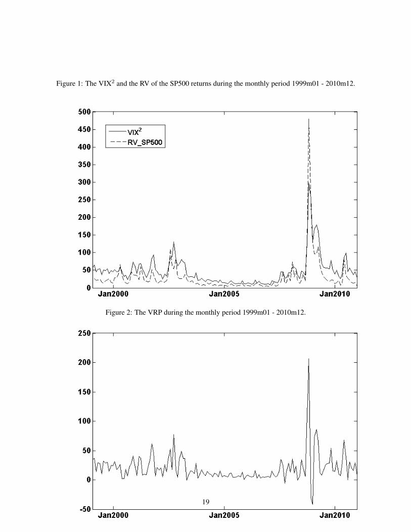
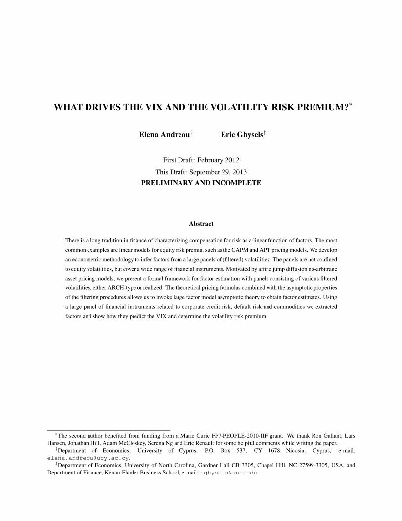
Figure 1: The VIX2 and the RV of the SP500 returns during the monthly period 1999m01 - 2010m12.

Figure 2: The VRP during the monthly period 1999m01 - 2010m12.

19

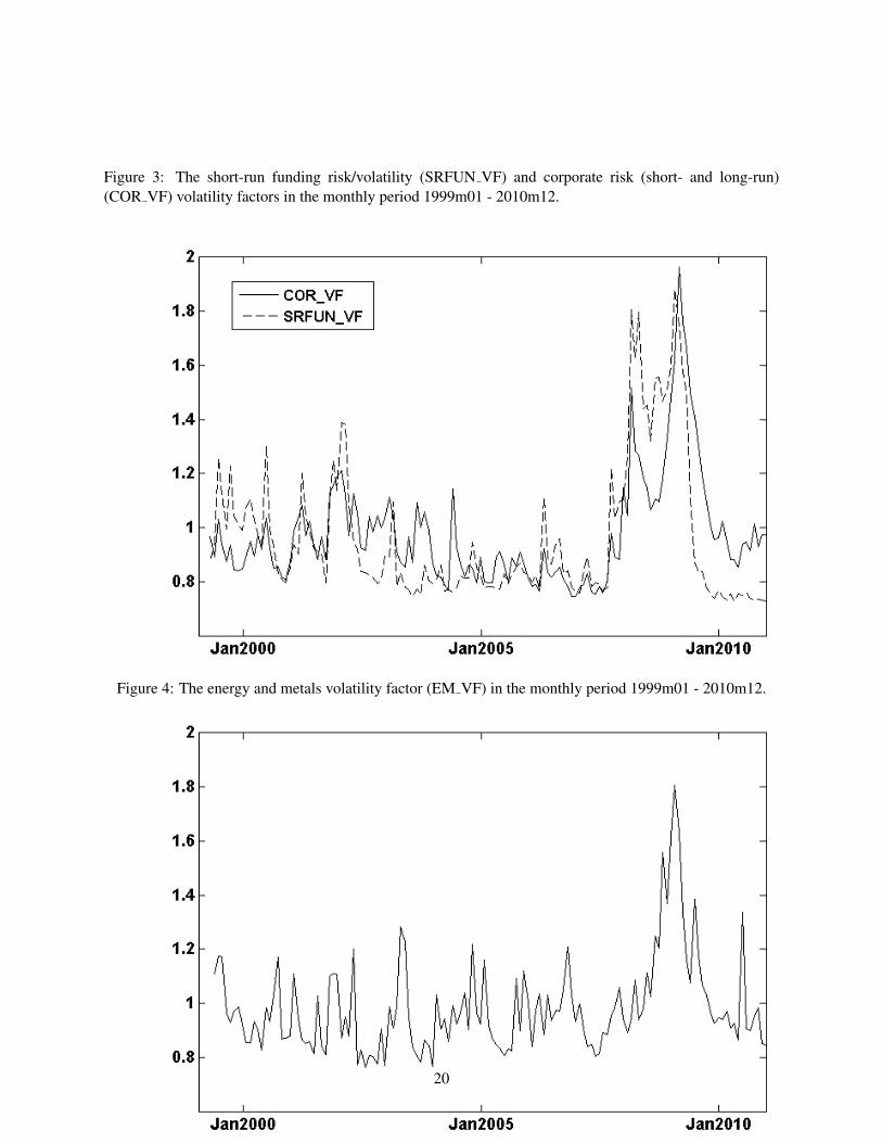
Figure 3: The short-run funding risk/volatility (SRFUN VF) and corporate risk (short- and long-run)(COR VF) volatility factors in the monthly period 1999m01 - 2010m12.

Figure 4: The energy and metals volatility factor (EM VF) in the monthly period 1999m01 - 2010m12.

20

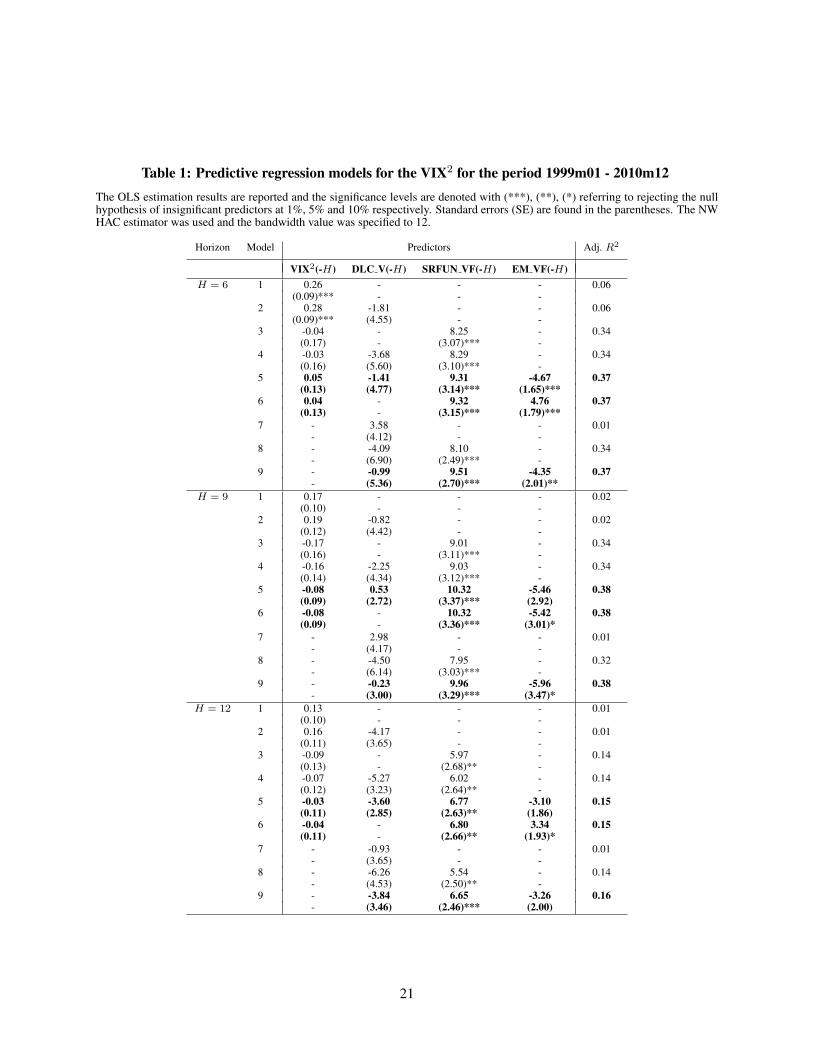
Table 1: Predictive regression models for the VIX2 for the period 1999m01 - 2010m12The OLS estimation results are reported and the significance levels are denoted with (***), (**), (*) referring to rejecting the nullhypothesis of insignificant predictors at 1%, 5% and 10% respectively. Standard errors (SE) are found in the parentheses. The NWHAC estimator was used and the bandwidth value was specified to 12.

Horizon Model Predictors Adj. R2

VIX2(-H) DLC V(-H) SRFUN VF(-H) EM VF(-H)H = 6 1 0.26 - - - 0.06

(0.09)*** - - -2 0.28 -1.81 - - 0.06

(0.09)*** (4.55) - -3 -0.04 - 8.25 - 0.34

(0.17) - (3.07)*** -4 -0.03 -3.68 8.29 - 0.34

(0.16) (5.60) (3.10)*** -5 0.05 -1.41 9.31 -4.67 0.37

(0.13) (4.77) (3.14)*** (1.65)***6 0.04 - 9.32 4.76 0.37

(0.13) - (3.15)*** (1.79)***7 - 3.58 - - 0.01

- (4.12) - -8 - -4.09 8.10 - 0.34

- (6.90) (2.49)*** -9 - -0.99 9.51 -4.35 0.37

- (5.36) (2.70)*** (2.01)**H = 9 1 0.17 - - - 0.02

(0.10) - - -2 0.19 -0.82 - - 0.02

(0.12) (4.42) - -3 -0.17 - 9.01 - 0.34

(0.16) - (3.11)*** -4 -0.16 -2.25 9.03 - 0.34

(0.14) (4.34) (3.12)*** -5 -0.08 0.53 10.32 -5.46 0.38

(0.09) (2.72) (3.37)*** (2.92)6 -0.08 - 10.32 -5.42 0.38

(0.09) - (3.36)*** (3.01)*7 - 2.98 - - 0.01

- (4.17) - -8 - -4.50 7.95 - 0.32

- (6.14) (3.03)*** -9 - -0.23 9.96 -5.96 0.38

- (3.00) (3.29)*** (3.47)*H = 12 1 0.13 - - - 0.01

(0.10) - - -2 0.16 -4.17 - - 0.01

(0.11) (3.65) - -3 -0.09 - 5.97 - 0.14

(0.13) - (2.68)** -4 -0.07 -5.27 6.02 - 0.14

(0.12) (3.23) (2.64)** -5 -0.03 -3.60 6.77 -3.10 0.15

(0.11) (2.85) (2.63)** (1.86)6 -0.04 - 6.80 3.34 0.15

(0.11) - (2.66)** (1.93)*7 - -0.93 - - 0.01

- (3.65) - -8 - -6.26 5.54 - 0.14

- (4.53) (2.50)** -9 - -3.84 6.65 -3.26 0.16

- (3.46) (2.46)*** (2.00)

21

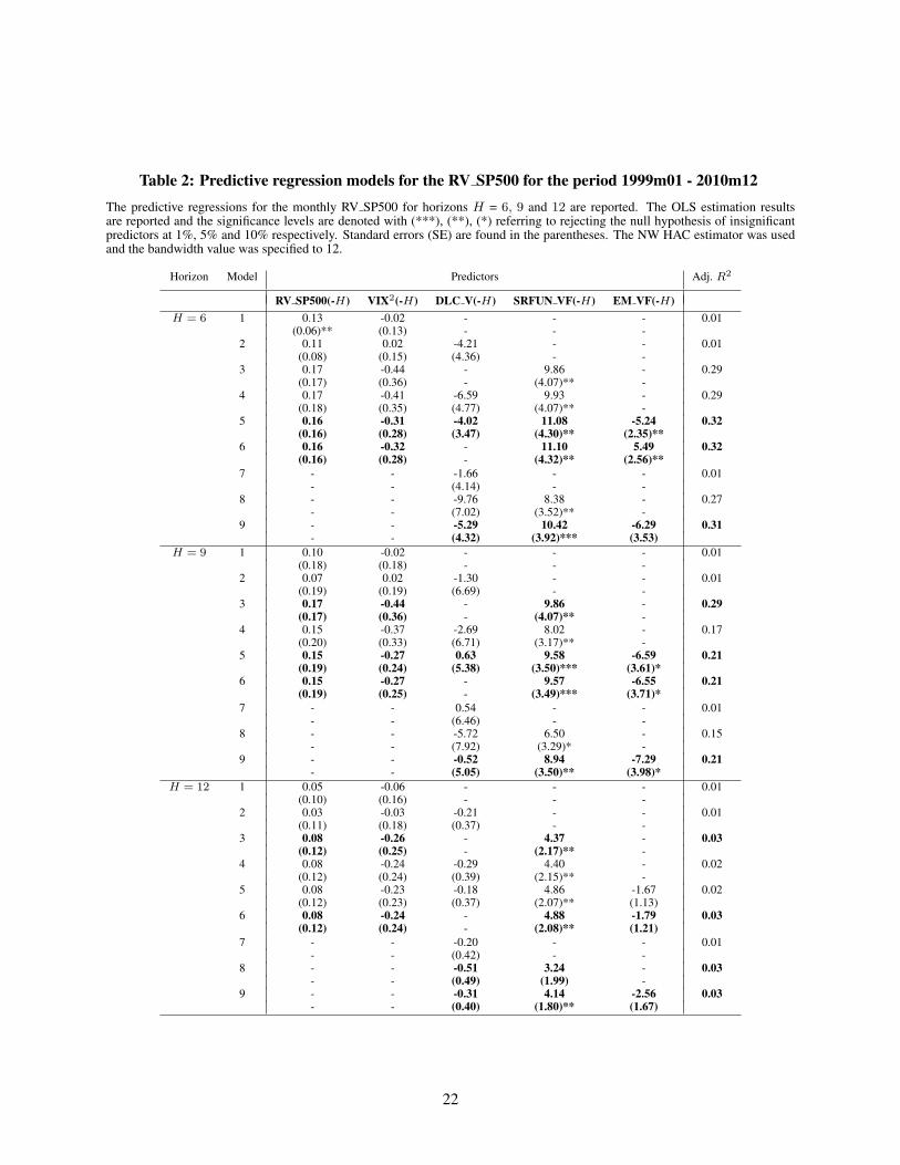
Table 2: Predictive regression models for the RV SP500 for the period 1999m01 - 2010m12The predictive regressions for the monthly RV SP500 for horizons H = 6, 9 and 12 are reported. The OLS estimation resultsare reported and the significance levels are denoted with (***), (**), (*) referring to rejecting the null hypothesis of insignificantpredictors at 1%, 5% and 10% respectively. Standard errors (SE) are found in the parentheses. The NW HAC estimator was usedand the bandwidth value was specified to 12.

Horizon Model Predictors Adj. R2

RV SP500(-H) VIX2(-H) DLC V(-H) SRFUN VF(-H) EM VF(-H)H = 6 1 0.13 -0.02 - - - 0.01

(0.06)** (0.13) - - -2 0.11 0.02 -4.21 - - 0.01

(0.08) (0.15) (4.36) - -3 0.17 -0.44 - 9.86 - 0.29

(0.17) (0.36) - (4.07)** -4 0.17 -0.41 -6.59 9.93 - 0.29

(0.18) (0.35) (4.77) (4.07)** -5 0.16 -0.31 -4.02 11.08 -5.24 0.32

(0.16) (0.28) (3.47) (4.30)** (2.35)**6 0.16 -0.32 - 11.10 5.49 0.32

(0.16) (0.28) - (4.32)** (2.56)**7 - - -1.66 - - 0.01

- - (4.14) - -8 - - -9.76 8.38 - 0.27

- - (7.02) (3.52)** -9 - - -5.29 10.42 -6.29 0.31

- - (4.32) (3.92)*** (3.53)H = 9 1 0.10 -0.02 - - - 0.01

(0.18) (0.18) - - -2 0.07 0.02 -1.30 - - 0.01

(0.19) (0.19) (6.69) - -3 0.17 -0.44 - 9.86 - 0.29

(0.17) (0.36) - (4.07)** -4 0.15 -0.37 -2.69 8.02 - 0.17

(0.20) (0.33) (6.71) (3.17)** -5 0.15 -0.27 0.63 9.58 -6.59 0.21

(0.19) (0.24) (5.38) (3.50)*** (3.61)*6 0.15 -0.27 - 9.57 -6.55 0.21

(0.19) (0.25) - (3.49)*** (3.71)*7 - - 0.54 - - 0.01

- - (6.46) - -8 - - -5.72 6.50 - 0.15

- - (7.92) (3.29)* -9 - - -0.52 8.94 -7.29 0.21

- - (5.05) (3.50)** (3.98)*H = 12 1 0.05 -0.06 - - - 0.01

(0.10) (0.16) - - -2 0.03 -0.03 -0.21 - - 0.01

(0.11) (0.18) (0.37) - -3 0.08 -0.26 - 4.37 - 0.03

(0.12) (0.25) - (2.17)** -4 0.08 -0.24 -0.29 4.40 - 0.02

(0.12) (0.24) (0.39) (2.15)** -5 0.08 -0.23 -0.18 4.86 -1.67 0.02

(0.12) (0.23) (0.37) (2.07)** (1.13)6 0.08 -0.24 - 4.88 -1.79 0.03

(0.12) (0.24) - (2.08)** (1.21)7 - - -0.20 - - 0.01

- - (0.42) - -8 - - -0.51 3.24 - 0.03

- - (0.49) (1.99) -9 - - -0.31 4.14 -2.56 0.03

- - (0.40) (1.80)** (1.67)

22

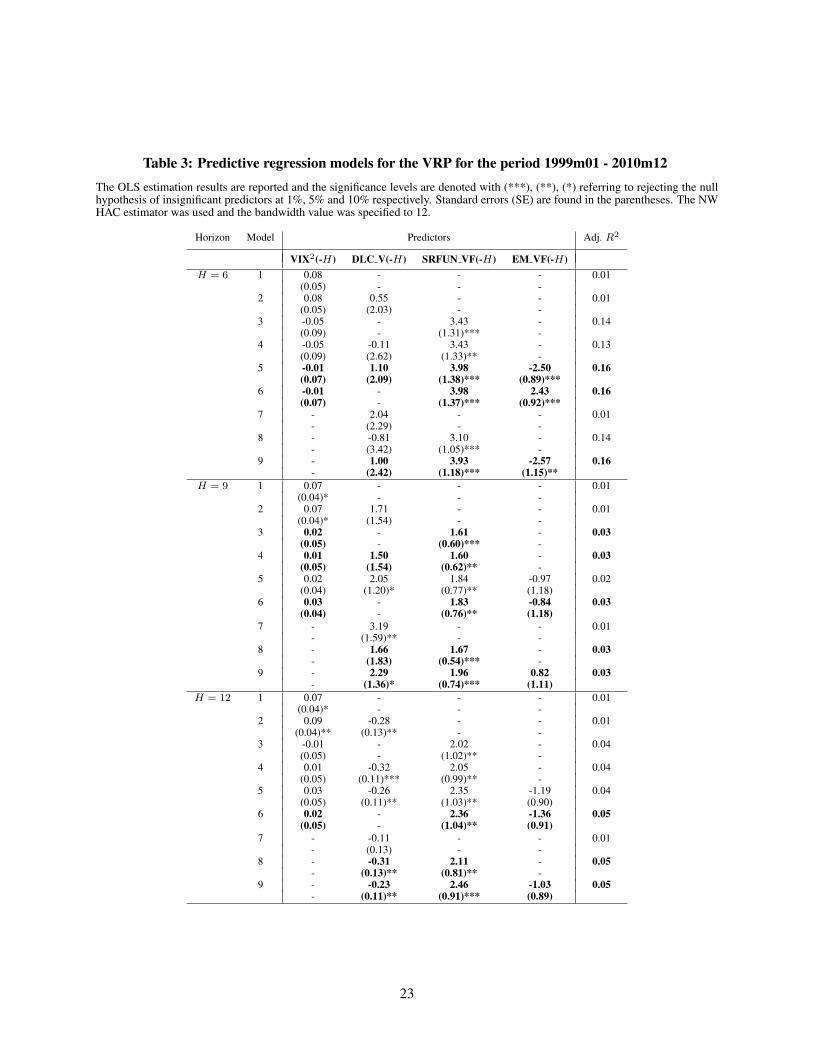
Table 3: Predictive regression models for the VRP for the period 1999m01 - 2010m12The OLS estimation results are reported and the significance levels are denoted with (***), (**), (*) referring to rejecting the nullhypothesis of insignificant predictors at 1%, 5% and 10% respectively. Standard errors (SE) are found in the parentheses. The NWHAC estimator was used and the bandwidth value was specified to 12.

Horizon Model Predictors Adj. R2

VIX2(-H) DLC V(-H) SRFUN VF(-H) EM VF(-H)H = 6 1 0.08 - - - 0.01

(0.05) - - -2 0.08 0.55 - - 0.01

(0.05) (2.03) - -3 -0.05 - 3.43 - 0.14

(0.09) - (1.31)*** -4 -0.05 -0.11 3.43 - 0.13

(0.09) (2.62) (1.33)** -5 -0.01 1.10 3.98 -2.50 0.16

(0.07) (2.09) (1.38)*** (0.89)***6 -0.01 - 3.98 2.43 0.16

(0.07) - (1.37)*** (0.92)***7 - 2.04 - - 0.01

- (2.29) - -8 - -0.81 3.10 - 0.14

- (3.42) (1.05)*** -9 - 1.00 3.93 -2.57 0.16

- (2.42) (1.18)*** (1.15)**H = 9 1 0.07 - - - 0.01

(0.04)* - - -2 0.07 1.71 - - 0.01

(0.04)* (1.54) - -3 0.02 - 1.61 - 0.03

(0.05) - (0.60)*** -4 0.01 1.50 1.60 - 0.03

(0.05) (1.54) (0.62)** -5 0.02 2.05 1.84 -0.97 0.02

(0.04) (1.20)* (0.77)** (1.18)6 0.03 - 1.83 -0.84 0.03

(0.04) - (0.76)** (1.18)7 - 3.19 - - 0.01

- (1.59)** - -8 - 1.66 1.67 - 0.03

- (1.83) (0.54)*** -9 - 2.29 1.96 0.82 0.03

- (1.36)* (0.74)*** (1.11)H = 12 1 0.07 - - - 0.01

(0.04)* - - -2 0.09 -0.28 - - 0.01

(0.04)** (0.13)** - -3 -0.01 - 2.02 - 0.04

(0.05) - (1.02)** -4 0.01 -0.32 2.05 - 0.04

(0.05) (0.11)*** (0.99)** -5 0.03 -0.26 2.35 -1.19 0.04

(0.05) (0.11)** (1.03)** (0.90)6 0.02 - 2.36 -1.36 0.05

(0.05) - (1.04)** (0.91)7 - -0.11 - - 0.01

- (0.13) - -8 - -0.31 2.11 - 0.05

- (0.13)** (0.81)** -9 - -0.23 2.46 -1.03 0.05

- (0.11)** (0.91)*** (0.89)

23

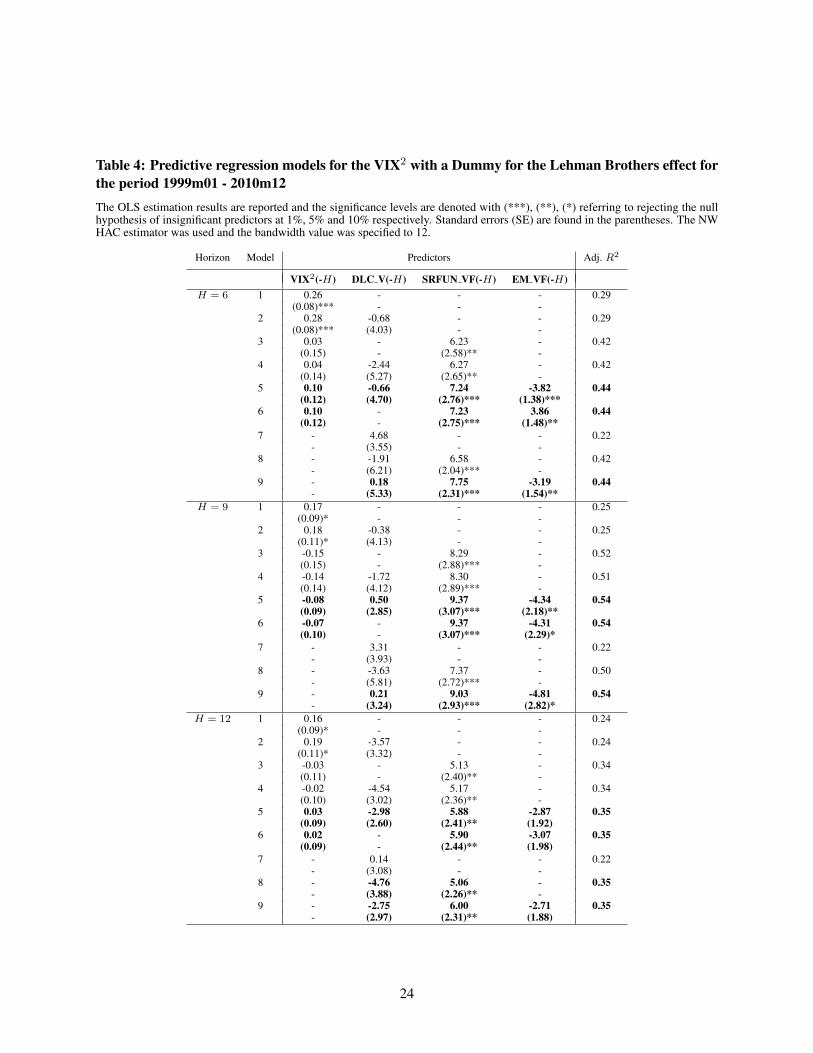
Table 4: Predictive regression models for the VIX2 with a Dummy for the Lehman Brothers effect forthe period 1999m01 - 2010m12The OLS estimation results are reported and the significance levels are denoted with (***), (**), (*) referring to rejecting the nullhypothesis of insignificant predictors at 1%, 5% and 10% respectively. Standard errors (SE) are found in the parentheses. The NWHAC estimator was used and the bandwidth value was specified to 12.

Horizon Model Predictors Adj. R2

VIX2(-H) DLC V(-H) SRFUN VF(-H) EM VF(-H)H = 6 1 0.26 - - - 0.29

(0.08)*** - - -2 0.28 -0.68 - - 0.29

(0.08)*** (4.03) - -3 0.03 - 6.23 - 0.42

(0.15) - (2.58)** -4 0.04 -2.44 6.27 - 0.42

(0.14) (5.27) (2.65)** -5 0.10 -0.66 7.24 -3.82 0.44

(0.12) (4.70) (2.76)*** (1.38)***6 0.10 - 7.23 3.86 0.44

(0.12) - (2.75)*** (1.48)**7 - 4.68 - - 0.22

- (3.55) - -8 - -1.91 6.58 - 0.42

- (6.21) (2.04)*** -9 - 0.18 7.75 -3.19 0.44

- (5.33) (2.31)*** (1.54)**H = 9 1 0.17 - - - 0.25

(0.09)* - - -2 0.18 -0.38 - - 0.25

(0.11)* (4.13) - -3 -0.15 - 8.29 - 0.52

(0.15) - (2.88)*** -4 -0.14 -1.72 8.30 - 0.51

(0.14) (4.12) (2.89)*** -5 -0.08 0.50 9.37 -4.34 0.54

(0.09) (2.85) (3.07)*** (2.18)**6 -0.07 - 9.37 -4.31 0.54

(0.10) - (3.07)*** (2.29)*7 - 3.31 - - 0.22

- (3.93) - -8 - -3.63 7.37 - 0.50

- (5.81) (2.72)*** -9 - 0.21 9.03 -4.81 0.54

- (3.24) (2.93)*** (2.82)*H = 12 1 0.16 - - - 0.24

(0.09)* - - -2 0.19 -3.57 - - 0.24

(0.11)* (3.32) - -3 -0.03 - 5.13 - 0.34

(0.11) - (2.40)** -4 -0.02 -4.54 5.17 - 0.34

(0.10) (3.02) (2.36)** -5 0.03 -2.98 5.88 -2.87 0.35

(0.09) (2.60) (2.41)** (1.92)6 0.02 - 5.90 -3.07 0.35

(0.09) - (2.44)** (1.98)7 - 0.14 - - 0.22

- (3.08) - -8 - -4.76 5.06 - 0.35

- (3.88) (2.26)** -9 - -2.75 6.00 -2.71 0.35

- (2.97) (2.31)** (1.88)

24

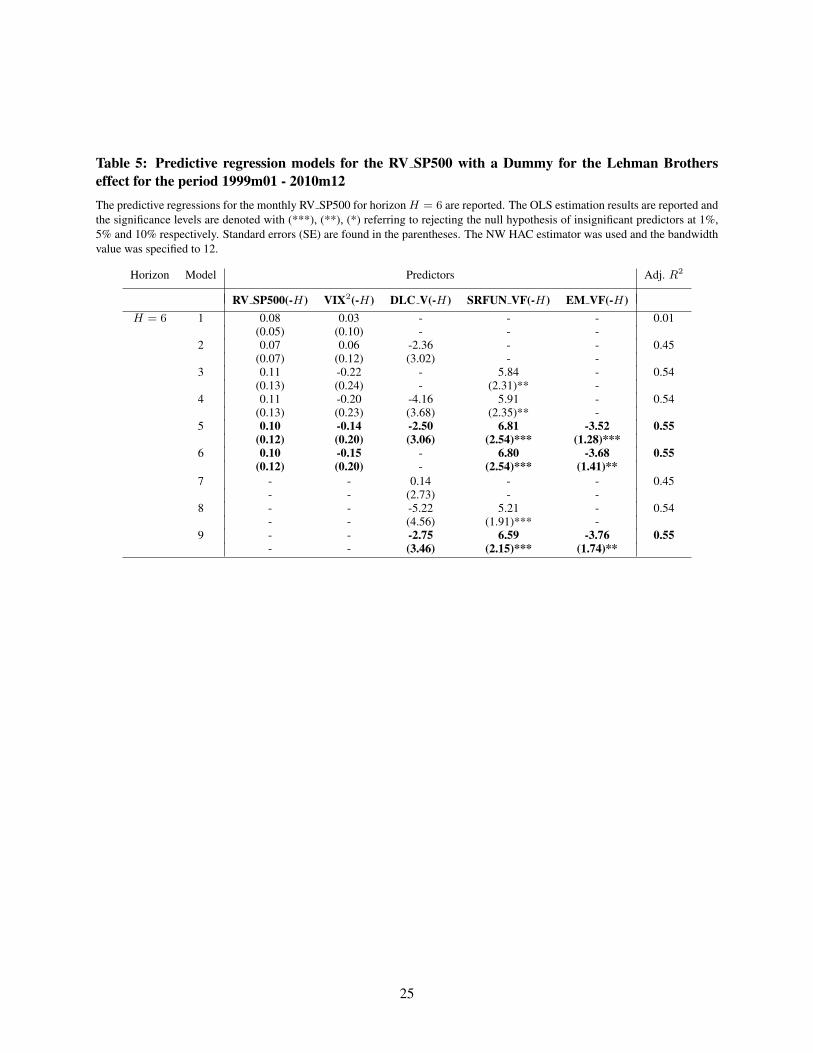
Table 5: Predictive regression models for the RV SP500 with a Dummy for the Lehman Brotherseffect for the period 1999m01 - 2010m12The predictive regressions for the monthly RV SP500 for horizon H = 6 are reported. The OLS estimation results are reported andthe significance levels are denoted with (***), (**), (*) referring to rejecting the null hypothesis of insignificant predictors at 1%,5% and 10% respectively. Standard errors (SE) are found in the parentheses. The NW HAC estimator was used and the bandwidthvalue was specified to 12.

Horizon Model Predictors Adj. R2

RV SP500(-H) VIX2(-H) DLC V(-H) SRFUN VF(-H) EM VF(-H)H = 6 1 0.08 0.03 - - - 0.01

(0.05) (0.10) - - -2 0.07 0.06 -2.36 - - 0.45

(0.07) (0.12) (3.02) - -3 0.11 -0.22 - 5.84 - 0.54

(0.13) (0.24) - (2.31)** -4 0.11 -0.20 -4.16 5.91 - 0.54

(0.13) (0.23) (3.68) (2.35)** -5 0.10 -0.14 -2.50 6.81 -3.52 0.55

(0.12) (0.20) (3.06) (2.54)*** (1.28)***6 0.10 -0.15 - 6.80 -3.68 0.55

(0.12) (0.20) - (2.54)*** (1.41)**7 - - 0.14 - - 0.45

- - (2.73) - -8 - - -5.22 5.21 - 0.54

- - (4.56) (1.91)*** -9 - - -2.75 6.59 -3.76 0.55

- - (3.46) (2.15)*** (1.74)**

25

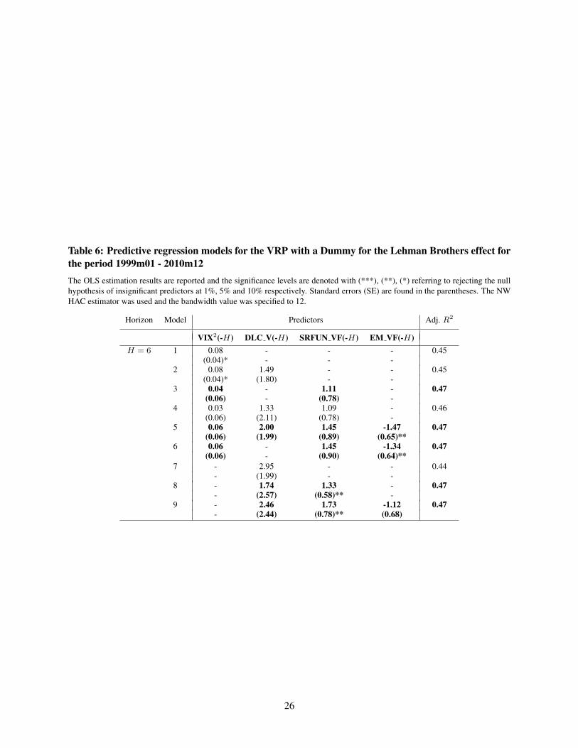
Table 6: Predictive regression models for the VRP with a Dummy for the Lehman Brothers effect forthe period 1999m01 - 2010m12The OLS estimation results are reported and the significance levels are denoted with (***), (**), (*) referring to rejecting the nullhypothesis of insignificant predictors at 1%, 5% and 10% respectively. Standard errors (SE) are found in the parentheses. The NWHAC estimator was used and the bandwidth value was specified to 12.

Horizon Model Predictors Adj. R2

VIX2(-H) DLC V(-H) SRFUN VF(-H) EM VF(-H)H = 6 1 0.08 - - - 0.45

(0.04)* - - -2 0.08 1.49 - - 0.45

(0.04)* (1.80) - -3 0.04 - 1.11 - 0.47

(0.06) - (0.78) -4 0.03 1.33 1.09 - 0.46

(0.06) (2.11) (0.78) -5 0.06 2.00 1.45 -1.47 0.47

(0.06) (1.99) (0.89) (0.65)**6 0.06 - 1.45 -1.34 0.47

(0.06) - (0.90) (0.64)**7 - 2.95 - - 0.44

- (1.99) - -8 - 1.74 1.33 - 0.47

- (2.57) (0.58)** -9 - 2.46 1.73 -1.12 0.47

- (2.44) (0.78)** (0.68)

26

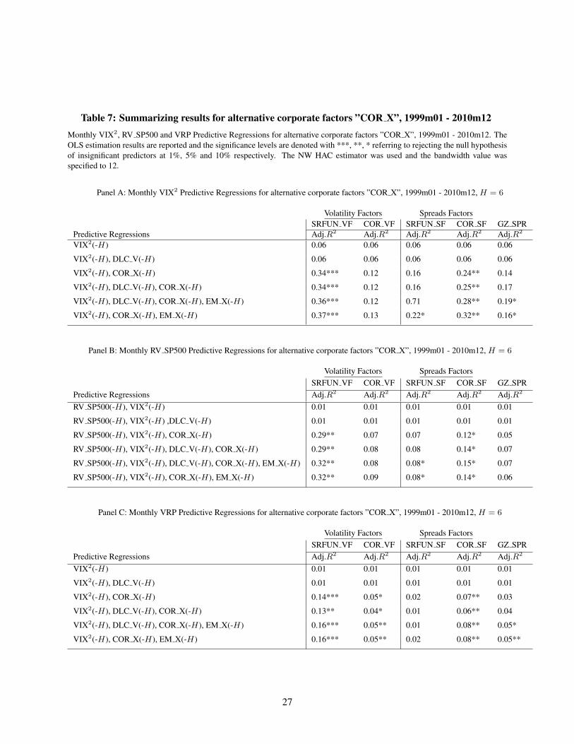
Table 7: Summarizing results for alternative corporate factors ”COR X”, 1999m01 - 2010m12Monthly VIX2, RV SP500 and VRP Predictive Regressions for alternative corporate factors ”COR X”, 1999m01 - 2010m12. TheOLS estimation results are reported and the significance levels are denoted with ***, **, * referring to rejecting the null hypothesisof insignificant predictors at 1%, 5% and 10% respectively. The NW HAC estimator was used and the bandwidth value wasspecified to 12.

Panel A: Monthly VIX2 Predictive Regressions for alternative corporate factors ”COR X”, 1999m01 - 2010m12, H = 6

Volatility Factors Spreads FactorsSRFUN VF COR VF SRFUN SF COR SF GZ SPR

Predictive Regressions Adj.R2 Adj.R2 Adj.R2 Adj.R2 Adj.R2

VIX2(-H) 0.06 0.06 0.06 0.06 0.06

VIX2(-H), DLC V(-H) 0.06 0.06 0.06 0.06 0.06

VIX2(-H), COR X(-H) 0.34*** 0.12 0.16 0.24** 0.14

VIX2(-H), DLC V(-H), COR X(-H) 0.34*** 0.12 0.16 0.25** 0.17

VIX2(-H), DLC V(-H), COR X(-H), EM X(-H) 0.36*** 0.12 0.71 0.28** 0.19*

VIX2(-H), COR X(-H), EM X(-H) 0.37*** 0.13 0.22* 0.32** 0.16*

Panel B: Monthly RV SP500 Predictive Regressions for alternative corporate factors ”COR X”, 1999m01 - 2010m12, H = 6

Volatility Factors Spreads FactorsSRFUN VF COR VF SRFUN SF COR SF GZ SPR

Predictive Regressions Adj.R2 Adj.R2 Adj.R2 Adj.R2 Adj.R2

RV SP500(-H), VIX2(-H) 0.01 0.01 0.01 0.01 0.01

RV SP500(-H), VIX2(-H) ,DLC V(-H) 0.01 0.01 0.01 0.01 0.01

RV SP500(-H), VIX2(-H), COR X(-H) 0.29** 0.07 0.07 0.12* 0.05

RV SP500(-H), VIX2(-H), DLC V(-H), COR X(-H) 0.29** 0.08 0.08 0.14* 0.07

RV SP500(-H), VIX2(-H), DLC V(-H), COR X(-H), EM X(-H) 0.32** 0.08 0.08* 0.15* 0.07

RV SP500(-H), VIX2(-H), COR X(-H), EM X(-H) 0.32** 0.09 0.08* 0.14* 0.06

Panel C: Monthly VRP Predictive Regressions for alternative corporate factors ”COR X”, 1999m01 - 2010m12, H = 6

Volatility Factors Spreads FactorsSRFUN VF COR VF SRFUN SF COR SF GZ SPR

Predictive Regressions Adj.R2 Adj.R2 Adj.R2 Adj.R2 Adj.R2

VIX2(-H) 0.01 0.01 0.01 0.01 0.01

VIX2(-H), DLC V(-H) 0.01 0.01 0.01 0.01 0.01

VIX2(-H), COR X(-H) 0.14*** 0.05* 0.02 0.07** 0.03

VIX2(-H), DLC V(-H), COR X(-H) 0.13** 0.04* 0.01 0.06** 0.04

VIX2(-H), DLC V(-H), COR X(-H), EM X(-H) 0.16*** 0.05** 0.01 0.08** 0.05*

VIX2(-H), COR X(-H), EM X(-H) 0.16*** 0.05** 0.02 0.08** 0.05**

27

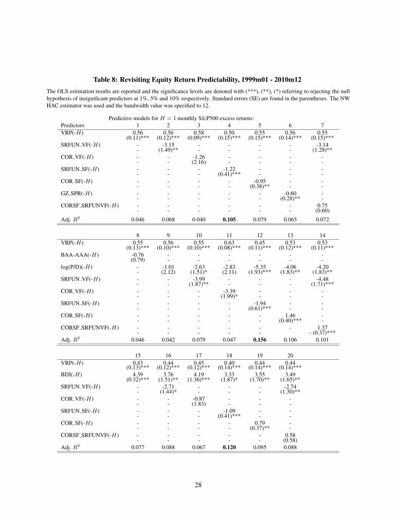
Table 8: Revisiting Equity Return Predictability, 1999m01 - 2010m12The OLS estimation results are reported and the significance levels are denoted with (***), (**), (*) referring to rejecting the nullhypothesis of insignificant predictors at 1%, 5% and 10% respectively. Standard errors (SE) are found in the parentheses. The NWHAC estimator was used and the bandwidth value was specified to 12.

Predictive models for H = 1 monthly S&P500 excess returns:Predictors 1 2 3 4 5 6 7VRP(-H) 0.56 0.56 0.58 0.50 0.55 0.56 0.55

(0.11)*** (0.12)*** (0.09)*** (0.15)*** (0.15)*** (0.14)*** (0.15)***SRFUN VF(-H) - -3.15 - - - - -3.14

- (1.49)** - - - - (1.28)**COR VF(-H) - - -1.26 - - - -

- - (2.16) - - - -SRFUN SF(-H) - - - -1.22 - - -

- - - (0.41)*** - - -COR SF(-H) - - - - -0.95 - -

- - - - (0.38)** - -GZ SPR(-H) - - - - - -0.60 -

- - - - - (0.28)** -CORSF SRFUNVF(-H) - - - - - - 0.75

- - - - - - (0.60)

Adj. R2 0.046 0.068 0.040 0.105 0.079 0.065 0.072

8 9 10 11 12 13 14VRP(-H) 0.55 0.56 0.55 0.63 0.45 0.53 0.53

(0.13)*** (0.10)*** (0.10)*** (0.08)*** (0.11)*** (0.12)*** (0.11)***BAA-AAA(-H) -0.76 - - - - - -

(0.79) - - - - - -log(P/D)(-H) - -1.01 -2.63 -2.83 -5.35 -4.06 -4.20

- (2.12) (1.51)* (2.11) (1.93)*** (1.83)** (1.83)**SRFUN VF(-H) - - -3.99 - - - -4.48

- - (1.87)** - - - (1.71)***COR VF(-H) - - - -3.39 - - -

- - - (1.99)* - - -SRFUN SF(-H) - - - - -1.94 - -

- - - - (0.61)*** - -COR SF(-H) - - - - - 1.46 -

- - - - - (0.40)*** -CORSF SRFUNVF(-H) - - - - - - 1.37

- - - - - - (0.37)***Adj. R2 0.046 0.042 0.079 0.047 0.156 0.106 0.101

15 16 17 18 19 20VRP(-H) 0.43 0.44 0.45 0.40 0.44 0.44

(0.13)*** (0.12)*** (0.12)*** (0.14)*** (0.14)*** (0.14)***BDI(-H) 4.39 3.76 4.19 3.33 3.55 3.49

(0.32)*** (1.51)** (1.36)*** (1.87)* (1.70)** (1.65)**SRFUN VF(-H) - -2.71 - - - -2.74

- (1.44)* - - - (1.30)**COR VF(-H) - - -0.87 - - -

- - (1.83) - - -SRFUN SF(-H) - - - -1.09 - -

- - - (0.41)*** - -COR SF(-H) - - - - 0.79 -

- - - - (0.37)** -CORSF SRFUNVF(-H) - - - - - 0.58

- - - - - (0.58)Adj. R2 0.077 0.088 0.067 0.120 0.095 0.088

28

References

A IT-SAHALIA, Y., M. KARAMAN, AND L. MANCINI (2012): “The term structure of variance swaps, riskpremia and the expectation hypothesis,” Discussion Paper, Princeton University.

AMENGUAL, D. (2009): “The term structure of variance risk premia,” Discussion Paper, PrincetonUniversity.

ANDREOU, E., AND E. GHYSELS (2013): “Estimating Volatility Risk Factors Using Large Panels ofFiltered or Realized Volatilities,” Discussion paper, UCY and UNC.

BAI, J. (2003): “Inferential theory for factor models of large dimensions,” Econometrica, 71, 135–171.

BAI, J., AND S. NG (2002): “Determining the number of factors in approximate factor models,”Econometrica, pp. 191–221.

BAKSHI, G., AND Z. CHEN (1997): “An alternative valuation model for contingent claims,” Journal ofFinancial Economics, 44, 123–165.

(2005): “Stock valuation in dynamic economies,” Journal of Financial Markets, 8, 111–151.

BAKSHI, G., G. PANAYOTOV, AND G. SKOULAKIS (2011): “Improving the predictability of real economicactivity and asset returns with forward variances inferred from option portfolios,” Journal of FinancialEconomics, 100, 475–495.

BALI, T., AND H. ZHOU (2012): “Risk, uncertainty, and expected returns,” Available at SSRN 2020604.

BANSAL, R., AND I. SHALIASTOVICH (2013): “A long-run risks explanation of predictability puzzles inbond and currency markets,” Review of Financial Studies, 26, 1–33.

BANSAL, R., AND A. YARON (2004): “Risks for the long run: A potential resolution of asset pricingpuzzles,” Journal of Finance, 59, 1481–1509.

BATES, D. S. (1996): “Jumps and stochastic volatility: Exchange rate processes implicit in Deutsche Markoptions,” Review of Financial Studies, 9, 69–107.

BEKAERT, G., E. ENGSTROM, AND S. R. GRENADIER (2010): “Stock and bond returns with MoodyInvestors,” Journal of Empirical Finance, 17, 867–894.

BEKAERT, G., E. ENGSTROM, AND Y. XING (2009): “Risk, uncertainty, and asset prices,” Journal ofFinancial Economics, 91, 59–82.

BEKAERT, G., AND S. R. GRENADIER (1999): “Stock and bond pricing in an affine economy,” Discussionpaper, National Bureau of Economic Research.

29

BOLLERSLEV, T., G. TAUCHEN, AND H. ZHOU (2009): “Expected stock returns and variance risk premia,”Review of Financial Studies, 22, 4463–4492.

BOLLERSLEV, T., AND V. TODOROV (2011): “Tails, fears, and risk premia,” Journal of Finance, 66, 2165–2211.

BRITTEN-JONES, M., AND A. NEUBERGER (2000): “Option prices, implied price processes, and stochasticvolatility,” Journal of Finance, 55, 839–866.

BUHLER, H. (2006): “Consistent variance curve models,” Finance and Stochastics, 10, 178–203.

CAMPBELL, J., AND R. SHILLER (1991): “Yield spreads and interest rate movements: A bird’s eye view,”Review of Economic Studies, 58, 495–514.

CARR, P., AND L. WU (2009): “Variance risk premiums,” Review of Financial Studies, 22, 1311–1341.

CHAMBERLAIN, G., AND M. ROTHSCHILD (1983): “Arbitrage, Factor Structure, and Mean-VarianceAnalysis on Large Asset Markets,” Econometrica, pp. 1281–1304.

CHRISTIANSEN, C., M. SCHMELING, AND A. SCHRIMPF (2012): “A comprehensive look at financialvolatility prediction by economic variables,” Journal of Applied Econometrics, 27, 956–977.

COCHRANE, J., AND M. PIAZZESI (2005): “Bond Risk Premia,” American Economic Review, pp. 138–160.

CONNOR, G., AND R. A. KORAJCZYK (1986): “Performance measurement with the arbitrage pricingtheory: A new framework for analysis,” Journal of Financial Economics, 15, 373–394.

(1988): “Risk and return in an equilibrium APT: Application of a new test methodology,” Journalof Financial Economics, 21, 255–289.

CORRADI, V., W. DISTASO, AND A. MELE (2013): “Macroeconomic determinants of stock marketvolatility and volatility risk-premiums,” Journal of Monetary Economics (forthcoming).

DAI, Q., AND K. J. SINGLETON (2000): “Specification analysis of affine term structure models,” Journalof Finance, 55, 1943–1978.

DICKEY, D. A., AND W. A. FULLER (1981): “Likelihood ratio statistics for autoregressive time series witha unit root,” Econometrica, 49, 1057–1072.

DRECHSLER, I., AND A. YARON (2011): “What’s vol got to do with it,” Review of Financial Studies, 24,1–45.

DUFFEE, G. R. (2011): “Forecasting with the term structure: The role of no-arbitrage restrictions,”Discussion paper, Working paper, Johns Hopkins University, Department of Economics.

30

DUFFIE, D., AND R. KAN (1996): “A yield-factor model of interest rates,” Mathematical Finance, 6, 379–406.

DUFFIE, D., J. PAN, AND K. SINGLETON (2000): “Transform analysis and asset pricing for affine jump-diffusions,” Econometrica, 68, 1343–1376.

EGLOFF, D., M. LEIPPOLD, AND L. WU (2010): “The term structure of variance swap rates and optimalvariance swap investments,” Journal of Financial and Quantitative Analysis, 45, 1279–1310.

ENGLE, R., E. GHYSELS, AND B. SOHN (2013): “Stock Market Volatility and MacroeconomicFundamentals,” Review of Economics and Statistics (forthcoming).

ERAKER, B., AND I. SHALIASTOVICH (2008): “An equilibrium guide to designing affine pricing models,”Mathematical Finance, 18, 519–543.

FAMA, E., AND R. BLISS (1987): “The information in long-maturity forward rates,” American EconomicReview, pp. 680–692.

HESTON, S. L. (1993): “A closed-form solution for options with stochastic volatility with applications tobond and currency options,” Review of Financial Studies, 6, 327–343.

JACQUIER, E., N. G. POLSON, AND P. E. ROSSI (2002): “Bayesian analysis of stochastic volatilitymodels,” Journal of Business and Economic Statistics, 20, 69–87.

JIANG, G., AND Y. TIAN (2005): “The model-free implied volatility and its information content,” Reviewof Financial Studies, 18, 1305–1342.

KOIJEN, R., H. LUSTIG, AND S. VAN NIEUWERBURGH (2010): “The cross-section and time-series ofstock and bond returns,” Discussion Paper, National Bureau of Economic Research.

LETTAU, M., AND J. A. WACHTER (2011): “The term structures of equity and interest rates,” Journal ofFinancial Economics, 101, 90–113.

LUDVIGSON, S., AND S. NG (2009): “Macro factors in bond risk premia,” Review of Financial Studies,22(12), 5027–5067.

LUDVIGSON, S. C., AND S. NG (2007): “The empirical risk-return relation: A factor analysis approach,”Journal of Financial Economics, 83, 171–222.

MERTON, R. (1973): “An intertemporal capital asset pricing model,” Econometrica, pp. 867–887.

MUELLER, P., A. VEDOLIN, AND H. ZHOU (2011): “Short-run bond risk premia,” Available at SSRNhttp://papers.ssrn.com/sol3/papers.cfm?abstract_id=1851854.

NELSON, D. B. (1990): “ARCH models as diffusion approximations,” Journal of Econometrics, 45, 7–38.

31

(1996): “Asymptotic filtering theory for multivariate ARCH models,” Journal of Econometrics, 71,1–47.

NELSON, D. B., AND D. P. FOSTER (1994): “Asymptotic filtering theory for univariate ARCH models,”Econometrica, 62, 1–41.

PROTTER, P. (2004): Stochastic Integration and Differential Equations. Springer.

ROSS, S. (1976a): “The Arbitrage Theory of Capital Asset Pricing,” Journal of Economic Theory, 13,341–360.

ROSS, S. A. (1976b): “The arbitrage theory of capital asset pricing,” Journal of Economic Theory, 13,341–360.

STOCK, J., AND M. WATSON (2002): “Forecasting using principal components from a large number ofpredictors,” Journal of the American Statistical Association, 97, 1167–1179.

TODOROV, V. (2010): “Variance risk-premium dynamics: The role of jumps,” Review of Financial Studies,23, 345–383.

VASICEK, O. (1977): “An equilibrium characterization of the term structure,” Journal of FinancialEconomics, 5, 177–188.

WANG, H., H. ZHOU, AND Y. ZHOU (2013): “Credit default swap spreads and variance risk premia,”Journal of Banking and Finance (forthcoming).

ZHOU, H. (2010): “Variance risk premia, asset predictability puzzles, and macroeconomic uncertainty,”Available at http://papers.ssrn.com/sol3/papers.cfm?abstract_id=1400049.

32

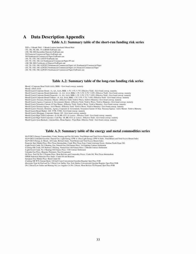
A Data Description AppendixTable A.1: Summary table of the short-run funding risk series

TED = 3 Month Tbill - 3 Month London Interbank Offered Rate(7D, 1M, 3M, 6M, 1Y) LIBOR-FedFunds rate(1M, 3M, 6M) Eurodollar Deposits-FedFunds rate1M Financial Commercial Paper-FedFunds rate1M Nonfinancial Commercial Paper-FedFunds rate(1D, 7D, 15D, 1M) AAFCP-FedFunds rate(1D, 7D, 15D, 1M) AA Nonfinancial Commercial Paper-FF rate(1M, 3M, 6M) Certificates of Deposit-FedFunds rate(1D, 7D, 15D, 1M) A2/P2/F2 Nonfinancial Commercial Paper-AA Nonfinancial Commercial Paper(1D, 7D, 15D, 1M) A2/P2/F2 Nonfinancial Commercial Paper-AA Financial Commercial Paper(1D, 7D, 15D, 1M) A2/P2/F2 Nonfinancial Commercial Paper-FedFunds rate

Table A.2: Summary table of the long-run funding risk seriesMoody’s Corporate Bond Yield (AAA, BBB) - Govt bond corresp. maturityMoody’s BAA-AAAMerrill Lynch Corporate Bonds: (A, AA, AAA, BBB, 1-3Y, 3-5Y, 5-7Y): Effective Yield - Govt bond corresp. maturityMerrill Lynch Corporate Bonds:Industrials: (A, AA, AAA, BBB, 1-3Y, 3-5Y, 5-7Y, 7-10Y): Effective Yield - Govt bond corresp. maturityMerrill Lynch Corporate Bonds:Financials: (A, AA, AAA, BBB, 1-3Y, 3-5Y, 5-7Y, 7-10Y): Effective Yield - Govt bond corresp. maturityMerrill Lynch Corporate Bonds:Utilities: (A, AA, AAA, BBB, 1-3Y, 3-5Y, 5-7Y, 7-10Y): Effective Yield - Govt bond corresp. maturityMerrill Lynch (Treasury, Domestic) Master: (Effective Yield, Yield to Worst, Yield to Maturity) -Govt bond corresp. maturityMerrill Lynch (Agency, Corporate & Government) Master: (Effective Yield, Yield to Worst, Yield to Maturity) -Govt bond corresp. maturityMerrill Lynch Treasuries Current 10 Year Master: (Effective Yield, Yield to Worst, Yield to Maturity) -Govt bond corresp. maturityMerrill Lynch Treasury/Agency: AAA Master: (Effective Yield, Yield to Worst, Yield to Maturity) -Govt bond corresp. maturityMerrill Lynch (Treasury, Domestic, Agency, Corporate & Government, Treasuries Current 10 Year, Treasury/Agency: AAA) Master: Yield to MaturityMerrill Lynch Broad Market: (Eff, YTW, YTM) -Govt bond corresp. maturityMerrill Lynch (Mortgage, Corporate) Master: Eff - Govt bond corresp. maturityMerrill Lynch High Yield Corporates: (Ii, B, BB, CCC & Lower) : Effective Yield - Govt bond corresp. maturityMerrill Lynch High Yield Corporates: Cash Pay: (B, BB, CCC & Lower) : Effective Yield - Govt bond corresp. maturityMerrill Lynch Asset-Backeds: (Automobiles, Home Equity): Fixed Rate: Effective Yield - Govt bond corresp. maturity

Table A.3: Summary table of the energy and metal commodities seriesS&P GSCI (Energy Commodities, Crude, Heating and Gas Oil) Index, Total Return and Total Excess Return IndexS&P GSCI (Unleaded Gasoline, Natural Gas, Light Energy CPW 4, Ultra-Light Energy CPW 8) Index, Total Return and Total Excess Return IndexS&P GSCI (Energy & Metals, All Crude, Biofuel) Index, Total Return and Total Excess Return IndexDomestic Spot Market Price (West Texas Intermediate, Crude West Texas Sour, Crude Louisiana Sweet, Alaskan North Slope Oil)(Light Sweet Crude, No 2 Heating, Gas, Natural Gas) Oil Futures Price: 1st Expiring Contract Settlement(Cushing OK Crude, NY Harbour 2 Heating, Natural Gas) Oil Futures Price: 2-Month Contract Settlement(Light Sweet Crude, No 2 Heating) Oil Futures Price: 3-M Contract SettlementUnleaded Gas Price, (Regular, Premium), Non-OxygenatedOil Price: Fuel Oil No 2, Propane Price: Mont Belvieu and Commodity Prices: Crude Oil, West Texas IntermediateFIBER Industrial Materials Price Index: Crude Oil and BenzeneEuropean Free Market Price: Brent Crude Oil(Cushing OK WTI, Europe Brent, US Gulf Coast Conventional Gasoline Regular) Spot Price FOB(Kerosene-Type Jet Fuel and No 2 Diesel Low Sulfur, New York Harbor Conventional Gasoline Regular) Spot Price FOB(No 2 Diesel Low Sulfur and Heating Oil, Los Angeles CA No 2 Diesel, Mont Belvieu TX Propane) Spot Price FOB

33

Table A.4: Detailed table of the short-run funding risk series

Index Definition Index Definition

1 15-Day A2/P2/F2 Nonfin. Com. Paper (% Per Annum) -15-Day Aa Fin. Com. Paper (% p.a) 19 15-Day Aa Nonfinancial Commercial Paper (% p.a) -FF

2 15-Day A2/P2/F2 Nonfin. Com. Paper (% p.a) -15-Day Aa Nonfin. Com. Paper (% p.a) 20 6-Month Eurodollar Deposits (London Bid) (% P.A.) -FF

3 7-Day London Interbank Offered Rate (%) -FF 21 6-Month Certificates Of Deposit, Secondary Market (% P.A.) -FF

4 1-Day Aa Nonfinancial Commercial Paper (% Per Annum) -FF 22 One-Year London Interbank Offered Rate (%) -FF

5 1-Day Aa Financial Commercial Paper (% Per Annum) -FF 23 1-Month Eurodollar Deposits (London Bid) (% P.A.) -FF

6 7-Day Aa Nonfinancial Commercial Paper (% Per Annum) -FF 24 1-Month A2/P2/F2 Nonfinancial Commercial Paper (% Per Annum) -FF

7 7-Day Aa Financial Commercial Paper (% Per Annum) -FF 25 3-Month Eurodollar Deposits (London Bid) (% P.A.) -FF

8 1-Day A2/P2/F2 Nonfinancial Commercial Paper (% Per Annum) -FF 26 3-Month London Interbank Offered Rate (%) -FF

9 15-Day Aa Financial Commercial Paper (% Per Annum) -FF 27 3-Month Certificates Of Deposit, Secondary Market (% P.A.) -FF

10 7-Day A2/P2/F2 Nonfin. Com. Paper (% Per Annum) -7-Day Aa Nonfin. Com. Paper (% p.a) 28 6-Month London Interbank Offered Rate (%) -FF

11 1-Month Nonfinancial Commercial Paper (% Per Annum) -FF 29 1-Month London Interbank Offered Rate (%) -FF

12 1-Month Aa Nonfinancial Commercial Paper (% Per Annum) -FF 30 7-Day A2/P2/F2 Nonfin. Com. Paper (% p.a) -7-Day Aa Fin. Com. Paper (% p.a)

13 1-Day A2/P2/F2 Nonfin. Com. Paper (% p.a) -1-Day Aa Fin. Com. Paper (% Per Annum) 31 Overnight London Interbank Offered Rate (%) -FF

14 1-Month Certificates Of Deposit, Secondary Market (% P.A.) -FF 32 Ted 3Month Tbill-3-Month London Interbank Offered Rate (%) -FF

15 7-Day A2/P2/F2 Nonfinancial Commercial Paper (% Per Annum) -FF 33 1-Month A2/P2/F2 Nonfin. Com. Paper (% p.a) -1-Month Aa Nonfin. Com. Paper

16 1-Month Financial Commercial Paper (% Per Annum) -FF 34 15-Day A2/P2/F2 Nonfinancial Commercial Paper (% Per Annum) -FF

17 1-Month Aa Financial Commercial Paper (% Per Annum) -FF 35 1-Month A2/P2/F2 Nonfin. Com. Paper (% p.a) -1-Month Aa Fin. Com. Paper (% p.a)

18 1-Day A2/P2/F2 Nonfin. Com. Paper (% Per Annum) -1-Day Aa Nonfin. Com. Paper (% p.a)

34

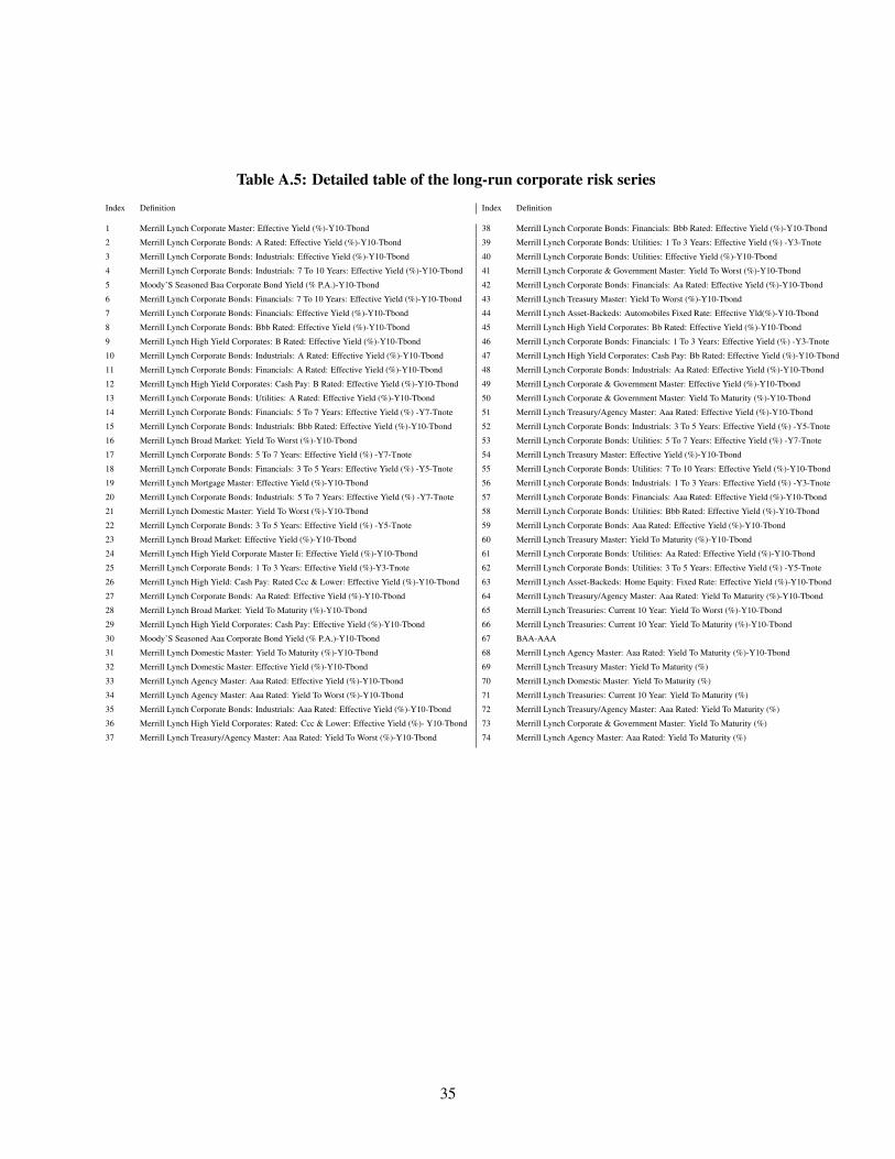
Table A.5: Detailed table of the long-run corporate risk series

Index Definition Index Definition

1 Merrill Lynch Corporate Master: Effective Yield (%)-Y10-Tbond 38 Merrill Lynch Corporate Bonds: Financials: Bbb Rated: Effective Yield (%)-Y10-Tbond

2 Merrill Lynch Corporate Bonds: A Rated: Effective Yield (%)-Y10-Tbond 39 Merrill Lynch Corporate Bonds: Utilities: 1 To 3 Years: Effective Yield (%) -Y3-Tnote

3 Merrill Lynch Corporate Bonds: Industrials: Effective Yield (%)-Y10-Tbond 40 Merrill Lynch Corporate Bonds: Utilities: Effective Yield (%)-Y10-Tbond

4 Merrill Lynch Corporate Bonds: Industrials: 7 To 10 Years: Effective Yield (%)-Y10-Tbond 41 Merrill Lynch Corporate & Government Master: Yield To Worst (%)-Y10-Tbond

5 Moody’S Seasoned Baa Corporate Bond Yield (% P.A.)-Y10-Tbond 42 Merrill Lynch Corporate Bonds: Financials: Aa Rated: Effective Yield (%)-Y10-Tbond

6 Merrill Lynch Corporate Bonds: Financials: 7 To 10 Years: Effective Yield (%)-Y10-Tbond 43 Merrill Lynch Treasury Master: Yield To Worst (%)-Y10-Tbond

7 Merrill Lynch Corporate Bonds: Financials: Effective Yield (%)-Y10-Tbond 44 Merrill Lynch Asset-Backeds: Automobiles Fixed Rate: Effective Yld(%)-Y10-Tbond

8 Merrill Lynch Corporate Bonds: Bbb Rated: Effective Yield (%)-Y10-Tbond 45 Merrill Lynch High Yield Corporates: Bb Rated: Effective Yield (%)-Y10-Tbond

9 Merrill Lynch High Yield Corporates: B Rated: Effective Yield (%)-Y10-Tbond 46 Merrill Lynch Corporate Bonds: Financials: 1 To 3 Years: Effective Yield (%) -Y3-Tnote

10 Merrill Lynch Corporate Bonds: Industrials: A Rated: Effective Yield (%)-Y10-Tbond 47 Merrill Lynch High Yield Corporates: Cash Pay: Bb Rated: Effective Yield (%)-Y10-Tbond

11 Merrill Lynch Corporate Bonds: Financials: A Rated: Effective Yield (%)-Y10-Tbond 48 Merrill Lynch Corporate Bonds: Industrials: Aa Rated: Effective Yield (%)-Y10-Tbond

12 Merrill Lynch High Yield Corporates: Cash Pay: B Rated: Effective Yield (%)-Y10-Tbond 49 Merrill Lynch Corporate & Government Master: Effective Yield (%)-Y10-Tbond

13 Merrill Lynch Corporate Bonds: Utilities: A Rated: Effective Yield (%)-Y10-Tbond 50 Merrill Lynch Corporate & Government Master: Yield To Maturity (%)-Y10-Tbond

14 Merrill Lynch Corporate Bonds: Financials: 5 To 7 Years: Effective Yield (%) -Y7-Tnote 51 Merrill Lynch Treasury/Agency Master: Aaa Rated: Effective Yield (%)-Y10-Tbond

15 Merrill Lynch Corporate Bonds: Industrials: Bbb Rated: Effective Yield (%)-Y10-Tbond 52 Merrill Lynch Corporate Bonds: Industrials: 3 To 5 Years: Effective Yield (%) -Y5-Tnote

16 Merrill Lynch Broad Market: Yield To Worst (%)-Y10-Tbond 53 Merrill Lynch Corporate Bonds: Utilities: 5 To 7 Years: Effective Yield (%) -Y7-Tnote

17 Merrill Lynch Corporate Bonds: 5 To 7 Years: Effective Yield (%) -Y7-Tnote 54 Merrill Lynch Treasury Master: Effective Yield (%)-Y10-Tbond

18 Merrill Lynch Corporate Bonds: Financials: 3 To 5 Years: Effective Yield (%) -Y5-Tnote 55 Merrill Lynch Corporate Bonds: Utilities: 7 To 10 Years: Effective Yield (%)-Y10-Tbond

19 Merrill Lynch Mortgage Master: Effective Yield (%)-Y10-Tbond 56 Merrill Lynch Corporate Bonds: Industrials: 1 To 3 Years: Effective Yield (%) -Y3-Tnote

20 Merrill Lynch Corporate Bonds: Industrials: 5 To 7 Years: Effective Yield (%) -Y7-Tnote 57 Merrill Lynch Corporate Bonds: Financials: Aaa Rated: Effective Yield (%)-Y10-Tbond

21 Merrill Lynch Domestic Master: Yield To Worst (%)-Y10-Tbond 58 Merrill Lynch Corporate Bonds: Utilities: Bbb Rated: Effective Yield (%)-Y10-Tbond

22 Merrill Lynch Corporate Bonds: 3 To 5 Years: Effective Yield (%) -Y5-Tnote 59 Merrill Lynch Corporate Bonds: Aaa Rated: Effective Yield (%)-Y10-Tbond

23 Merrill Lynch Broad Market: Effective Yield (%)-Y10-Tbond 60 Merrill Lynch Treasury Master: Yield To Maturity (%)-Y10-Tbond

24 Merrill Lynch High Yield Corporate Master Ii: Effective Yield (%)-Y10-Tbond 61 Merrill Lynch Corporate Bonds: Utilities: Aa Rated: Effective Yield (%)-Y10-Tbond

25 Merrill Lynch Corporate Bonds: 1 To 3 Years: Effective Yield (%)-Y3-Tnote 62 Merrill Lynch Corporate Bonds: Utilities: 3 To 5 Years: Effective Yield (%) -Y5-Tnote

26 Merrill Lynch High Yield: Cash Pay: Rated Ccc & Lower: Effective Yield (%)-Y10-Tbond 63 Merrill Lynch Asset-Backeds: Home Equity: Fixed Rate: Effective Yield (%)-Y10-Tbond

27 Merrill Lynch Corporate Bonds: Aa Rated: Effective Yield (%)-Y10-Tbond 64 Merrill Lynch Treasury/Agency Master: Aaa Rated: Yield To Maturity (%)-Y10-Tbond

28 Merrill Lynch Broad Market: Yield To Maturity (%)-Y10-Tbond 65 Merrill Lynch Treasuries: Current 10 Year: Yield To Worst (%)-Y10-Tbond

29 Merrill Lynch High Yield Corporates: Cash Pay: Effective Yield (%)-Y10-Tbond 66 Merrill Lynch Treasuries: Current 10 Year: Yield To Maturity (%)-Y10-Tbond

30 Moody’S Seasoned Aaa Corporate Bond Yield (% P.A.)-Y10-Tbond 67 BAA-AAA

31 Merrill Lynch Domestic Master: Yield To Maturity (%)-Y10-Tbond 68 Merrill Lynch Agency Master: Aaa Rated: Yield To Maturity (%)-Y10-Tbond

32 Merrill Lynch Domestic Master: Effective Yield (%)-Y10-Tbond 69 Merrill Lynch Treasury Master: Yield To Maturity (%)

33 Merrill Lynch Agency Master: Aaa Rated: Effective Yield (%)-Y10-Tbond 70 Merrill Lynch Domestic Master: Yield To Maturity (%)

34 Merrill Lynch Agency Master: Aaa Rated: Yield To Worst (%)-Y10-Tbond 71 Merrill Lynch Treasuries: Current 10 Year: Yield To Maturity (%)

35 Merrill Lynch Corporate Bonds: Industrials: Aaa Rated: Effective Yield (%)-Y10-Tbond 72 Merrill Lynch Treasury/Agency Master: Aaa Rated: Yield To Maturity (%)

36 Merrill Lynch High Yield Corporates: Rated: Ccc & Lower: Effective Yield (%)- Y10-Tbond 73 Merrill Lynch Corporate & Government Master: Yield To Maturity (%)

37 Merrill Lynch Treasury/Agency Master: Aaa Rated: Yield To Worst (%)-Y10-Tbond 74 Merrill Lynch Agency Master: Aaa Rated: Yield To Maturity (%)

35

Table A.6: Detailed table of the energy and metal Commodities

Index Definition Index Definition

1 Lme Lead: Closing 3-Month Forward Price ($/Metric Tonne) 62 Lme Aluminum, 99.7% Purity: Closing Cash Price ($/Metric Tonne)

2 S&P GSCI Lead Total Return Index (Dec-30-94=100) 63 S&P GSCI All Crude Total Return Index (Dec-31-86=100)

3 S&P GSCI Lead Total Excess Return Index (Dec-30-94=100) 64 S&P GSCI Petroleum Ex-Gasoil Total Excess Return Index (Dec-30-82=100)

4 S&P GSCI Lead Index (Dec-30-94=100) 65 Cushing Ok Wti Spot Price Fob (Dollars Per Barrel)

5 S&P GSCI Zinc Index (Dec-31=90=100) 66 S&P GSCI Energy And Metals Index (Jan-6-95=100)

6 S&P GSCI Zinc Total Return Index (Dec-31=90=100) 67 Light Sweet Crude Oil Futures Price: 1St Expiring Contract Settlement ($/Bbl)

7 S&P GSCI Zinc Total Excess Return Index (Dec-31=90=100) 68 S&P GSCI Crude Oil Index

8 S&P GSCI Precious Metal Nearby Index (Jan-2-73=100) 69 S&P GSCI Crude Oil Total Excess Return Index

9 S&P GSCI Precious Metals Total Return Index (Dec-29-72=100) 70 S&P GSCI Crude Oil Total Return Index

10 S&P GSCI Silver Total Return Index (Dec-29-72=100) 71 Domestic Spot Market Price: Crude West Texas Sour, Midland ($/Barrel)

11 Lme Zinc: Closing Cash Price ($/Metric Tonne) 72 Domestic Spot Market Price: West Texas Intermediate, Cushing ($/Barrel)

12 S&P GSCI Silver Total Excess Return Index (Dec-29-72=100) 73 Commodity Prices: Aluminum, Lme Spot ($/Metric Ton)

13 S&P GSCI Biofuel Index (Jan-16-95=100) 74 S&P GSCI Energy Commodities Nearby Index (12/31/82100)

14 S&P GSCI Silver Index (Dec-29-72=100) 75 S&P GSCI Energy Commodities Total Return Index (12/31/82=100)

15 Commodity Prices: Zinc, Special High Grade (Cents/Lb) 76 S&P GSCI Four Energy Commodities Excess Return Index (Jan-16-95=100)

16 S&P GSCI Precious Metals Total Excess Return Index (Dec-29-72=100) 77 Commodity Prices: Copper Scrap, NY No. 2 (Cents/Lb)

17 S&P GSCI Biofuel Total Excess Return Index (Jan-16-95=100) 78 S&P GSCI Four Energy Commodities Index (Jan-16-95=100)

18 S&P GSCI Biofuel Total Return Index (Jan-16-95=100) 79 S&P GSCI Four Energy Commodities Total Return Index (Jan-16-95=100)

19 Fiber Industrial Materials Price Index: Metals (1990100) 80 Commodity Prices: Crude Oil, West Texas Intermediate ($/Barrel)

20 S&P GSCI Ultra-Light Energy Cpw 8 Total Return Index (Jan=2-70=100) 81 Commodity Prices: Tallow, Chicago Inedible Prime (Cents/Lb)

21 S&P GSCI Ultra-Light Energy Cpw 8 Excess Return Index (Jan=2-70=100) 82 Us Gulf Coast Conventional Gasoline Regular Spot Price Fob (Cents Per Gallon)

22 Lme Tin: Closing 3-Month Forward Price ($/Metric Tonne) 83 Domestic Spot Market Price: Crude Louisiana Sweet, St James ($/Barrel)

23 Philadelphia Semiconductor Index (12/01/93=100) 84 Europe Brent Spot Price Fob (Dollars Per Barrel)

24 S&P GSCI Gold Index 85 S&P GSCI Heating Oil Total Excess Return Index (Dec-31-82=100)

25 Lme Tin: Closing Cash Price ($/Metric Tonne) 86 S&P GSCI Natural Gas Total Excess Return Index (Dec-31-93=100)

26 S&P GSCI Gold Total Return Index 87 S&P GSCI Natural Gas Total Return Index (Dec-31-93=100)

27 Crb Spot Commodity Price Index: Metals (1967100) 88 Domestic Spot Mkt Price: Alaskan North Slope Oil Delivered Pacific ($/Barrel)

28 Gold Futures Price: 6-Month Contract Settlement ($/Troy Oz) 89 S&P GSCI Heating Oil Total Return Index (Dec-31-82=100)

29 S&P GSCI Gold Total Excess Return Index 90 Commodity Prices: Steel Scrap, No. 1 Heavy Melting ($/gross Ton)

30 Lme Nickel: Closing Cash Price ($/Metric Tonne) 91 Spot Price: U.S. Gulf Coast Kerosene-Type Jet Fuel F.O.B. (Cents/Gallon)

31 Cash Price: London Gold Bullion, Pm Fix (Us$/Troy Oz) 92 European Free Market Price: Brent Crude Oil ($/Barrel)

32 S&P GSCI Industrial Metals Nearby Index (Dec-31-76) 93 Mont Belvieu Tx Propane Spot Price Fob (Cents Per Gallon)

33 S&P GSCI Ultra-Light Energy Index Cpw 8 (Jan=2-70=100) 94 Random Lengths’ Framing Lumber Composite ($/1000 Bd Ft)

34 S&P GSCI Industrial Metals Total Return Index (Dec-31-76) 95 Unleaded Gas Price, Premium Non-Oxygenated, Ny ($/Gal)

35 S&P GSCI Industrial Metals Total Excess Return Index (Dec-31-76) 96 S&P GSCI Gasoil Total Excess Return Index

36 S&P GSCI Light Energy Cpw 4 Total Excess Return Index (Jan-02-70=100) 97 New York Harbor No 2 Diesel Low Sulfur Spot Price Fob (Cents Per Gallon)

37 S&P GSCI Light Energy Cpw 4 Total Return Index (Jan-02-70=100) 98 S&P GSCI Gasoil Total Return Index

38 S&P Gsci Nickel Total Return Index (Dec-31-92=100) 99 New York Harbor No 2 Heating Oil Spot Price Fob (Cents Per Gallon)

39 Lme Copper, Grade A: Closing Cash Price ($/Metric Tonne) 100 Ny Harbor #2 Heating Oil Futures Price: 2-Month Contract Settlement($/Gallon)

40 Lme Copper, Grade A: Closing 3-Month Forward Price ($/Metric Tonne) 101 S&P GSCI Heating Oil Index (Dec-31-82100)

41 Lme Nickel: Closing 3-Month Forward Price ($/Metric Tonne) 102 S&P GSCI Unleaded Gasoline Total Excess Return Index (Dec-31-87=100)

42 S&P GSCI Nickel Index (Dec-31-92=100) 103 S&P GSCI Unleaded Gasoline Total Return Index (Dec-31-87=100)

43 Commodity Prices: Benzene ($/Gal) 104 Commodity Prices: Random Lengths’ Structural Panel Composite ($/1000 Sq Ft)

44 S&P GSCI Copper Index (Dec-30-76=100) 105 Us Gulf Coast No 2 Diesel Low Sulfur Spot Price Fob (Cents Per Gallon)

45 S&P GSCI Copper Total Return Index (Dec-30-76=100) 106 S&P GSCI Natural Gas Index (Dec-31-93=100)

46 S&P GSCI Copper Total Excess Return Index (Dec-30-76=100) 107 Natural Gas Futures Price: 1St Expiring Contract Settlement ($/Mmbtu)

47 Lme Aluminum, 99.7% Purity: Closing 3-Month Forward Price ($Metric/Tonne) 108 S&P GSCI Unleaded Gasoline Index (Dec-31-87100)48 S&P GSCI Light Energy Index -Cpw 4 (Jan-02-70=100) 109 Philadelphia Exchange: Gold & Silver Index (Close, 6/7/89=90)

49 Commodity Prices: Hides, Chicago, Heavy Native Steers (Cents/Lb) 110 Gas Oil Futures Price: 1St Expiring Contract Settlement ($/Metric Ton)

50 Commodity Prices: Burlap, NY 10 Oz, 40 (Cents/Yard) 111 Natural Gas Futures Price: 2-Month Contract Settlement ($/Mmbtu)

51 Cushing Ok Crude Oil Futures Price: 2-Month Contract Settlement ($/Barrel) 112 S&P GSCI Gasoil Index

52 Light Sweet Crude Oil Futures Price: 3-Month Contract Settlement ($/Bbl) 113 Oil Price: Fuel Oil No 2, Ny ($/Gallon)

53 S&P GSCI Aluminum Total Excess Return Index (Dec-31-90=100) 114 Fiber Industrial Materials Price Index: Crude Oil And Benzene (1990100)

54 S&P GSCI Aluminum Total Return Index (Dec-31-90=100) 115 Los Angeles Ca No 2 Diesel Spot Price Fob (Cents Per Gallon)

55 S&P GSCI Aluminum Index (Dec-31-90=100) 116 Lme Aluminum Alloy: Closing 3-Month Forward Price ($/Metric Tonne)

56 S&P GSCI All Crude Index (Dec-31-86=100) 117 No 2 Heating Oil Futures Price: 3-Month Contract Settlement ($/Gal)

57 S&P GSCI Brent Crude Total Excess Return Index (Jan-6-99=100) 118 No 2 Heating Oil Futures Price: 1St Expiring Contract Settlement ($/Gal)

58 S&P GSCI Energy And Metals Total Excess Return Index (Jan-6-95=100) 119 Propane Price, Mont Belvieu ($/Gal)

59 S&P GSCI Brent Crude Total Return Index (Jan-6-99=100) 120 Lme Aluminum Alloy: Closing Cash Price ($/Metric Tonne)

60 S&P GSCI Energy And Metals Total Return Index (Jan-6-95=100) 121 Unleaded Gas Price, Regular, Non-Oxygenated, Ny ($/Gal)

61 S&P GSCI All Crude Total Excess Return Index (Dec-31-86=100) 122 New York Harbor Conventional Gasoline Regular Spot Price Fob (Cents Per Gallon)36

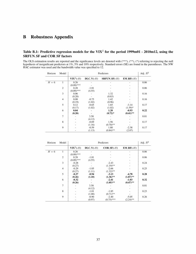
B Robustness Appendix

Table B.1: Predictive regression models for the VIX2 for the period 1999m01 - 2010m12, using theSRFUN SF and COR SF factorsThe OLS estimation results are reported and the significance levels are denoted with (***), (**), (*) referring to rejecting the nullhypothesis of insignificant predictors at 1%, 5% and 10% respectively. Standard errors (SE) are found in the parentheses. The NWHAC estimator was used and the bandwidth value was specified to 12.

Horizon Model Predictors Adj. R2

VIX2(-H) DLC V(-H) SRFUN SF(-H) EM RF(-H)H = 6 1 0.26 - - - 0.06

(0.09)*** - - -2 0.28 -1.81 - - 0.06

(0.09)*** (4.55) - -3 0.06 - 1.32 - 0.16

(0.20) - (0.83) -4 0.08 -0.75 1.42 - 0.16

(0.19) (1.02) (0.96) -5 0.12 -0.65 1.65 -3.14 0.17

(0.17) (1.02) (1.02) (1.59)*6 0.04 - 1.20 -0.93 0.22

(0.20) - (0.72)* (0.41)**7 - 3.58 - - 0.01

- (4.12) - -8 - -0.69 1.56 - 0.17

- (1.16) (0.70)** -9 - -0.59 1.80 -2.38 0.17

- (1.13) (0.84)** (2.07)

Horizon Model Predictors Adj. R2

VIX2(-H) DLC V(-H) COR SF(-H) EM RF(-H)H = 6 1 0.26 - - - 0.06

(0.09)*** - - -2 0.28 -1.81 - - 0.06

(0.09)*** (4.55) - -3 -0.28 - -2.43 - 0.24

(0.27) - (1.19)** -4 -0.29 -1.05 -2.66 - 0.25

(0.27) (1.11) (1.32)** -5 -0.27 -0.94 -3.13 -4.78 0.28

(0.26) (1.10) (1.36)** (1.87)**6 -0.32 - -2.41 -1.03 0.32

(0.26) - (1.05)** (0.47)**7 - 3.58 - - 0.01

- (4.12) - -8 - -1.01 -1.85 - 0.23

- (1.00) (0.71)** -9 - -0.90 -2.40 -5.05 0.26

- (0.97) (0.75)*** (2.24)**

37

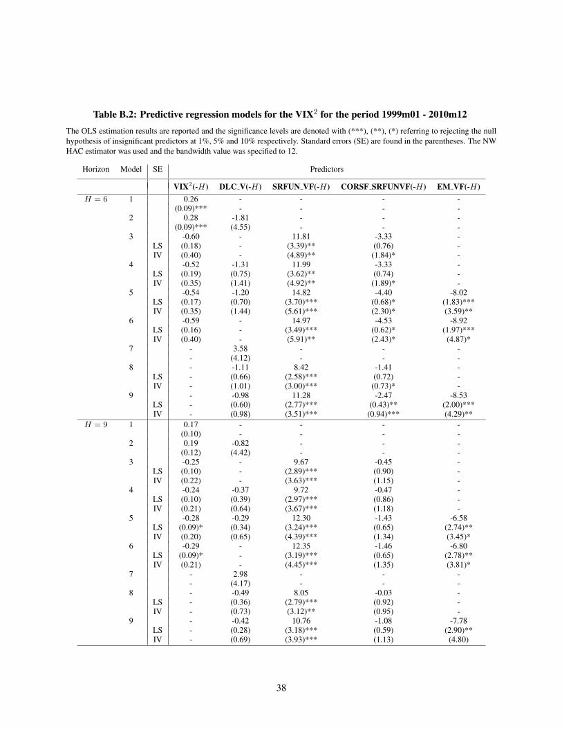
Table B.2: Predictive regression models for the VIX2 for the period 1999m01 - 2010m12The OLS estimation results are reported and the significance levels are denoted with (***), (**), (*) referring to rejecting the nullhypothesis of insignificant predictors at 1%, 5% and 10% respectively. Standard errors (SE) are found in the parentheses. The NWHAC estimator was used and the bandwidth value was specified to 12.

Horizon Model SE Predictors

VIX2(-H) DLC V(-H) SRFUN VF(-H) CORSF SRFUNVF(-H) EM VF(-H)H = 6 1 0.26 - - - -

(0.09)*** - - - -2 0.28 -1.81 - - -

(0.09)*** (4.55) - - -3 -0.60 - 11.81 -3.33 -

LS (0.18) - (3.39)** (0.76) -IV (0.40) - (4.89)** (1.84)* -

4 -0.52 -1.31 11.99 -3.33 -LS (0.19) (0.75) (3.62)** (0.74) -IV (0.35) (1.41) (4.92)** (1.89)* -

5 -0.54 -1.20 14.82 -4.40 -8.02LS (0.17) (0.70) (3.70)*** (0.68)* (1.83)***IV (0.35) (1.44) (5.61)*** (2.30)* (3.59)**

6 -0.59 - 14.97 -4.53 -8.92LS (0.16) - (3.49)*** (0.62)* (1.97)***IV (0.40) - (5.91)** (2.43)* (4.87)*

7 - 3.58 - - -- (4.12) - - -

8 - -1.11 8.42 -1.41 -LS - (0.66) (2.58)*** (0.72) -IV - (1.01) (3.00)*** (0.73)* -

9 - -0.98 11.28 -2.47 -8.53LS - (0.60) (2.77)*** (0.43)** (2.00)***IV - (0.98) (3.51)*** (0.94)*** (4.29)**

H = 9 1 0.17 - - - -(0.10) - - - -

2 0.19 -0.82 - - -(0.12) (4.42) - - -

3 -0.25 - 9.67 -0.45 -LS (0.10) - (2.89)*** (0.90) -IV (0.22) - (3.63)*** (1.15) -

4 -0.24 -0.37 9.72 -0.47 -LS (0.10) (0.39) (2.97)*** (0.86) -IV (0.21) (0.64) (3.67)*** (1.18) -

5 -0.28 -0.29 12.30 -1.43 -6.58LS (0.09)* (0.34) (3.24)*** (0.65) (2.74)**IV (0.20) (0.65) (4.39)*** (1.34) (3.45)*

6 -0.29 - 12.35 -1.46 -6.80LS (0.09)* - (3.19)*** (0.65) (2.78)**IV (0.21) - (4.45)*** (1.35) (3.81)*

7 - 2.98 - - -- (4.17) - - -

8 - -0.49 8.05 -0.03 -LS - (0.36) (2.79)*** (0.92) -IV - (0.73) (3.12)** (0.95) -

9 - -0.42 10.76 -1.08 -7.78LS - (0.28) (3.18)*** (0.59) (2.90)**IV - (0.69) (3.93)*** (1.13) (4.80)

38

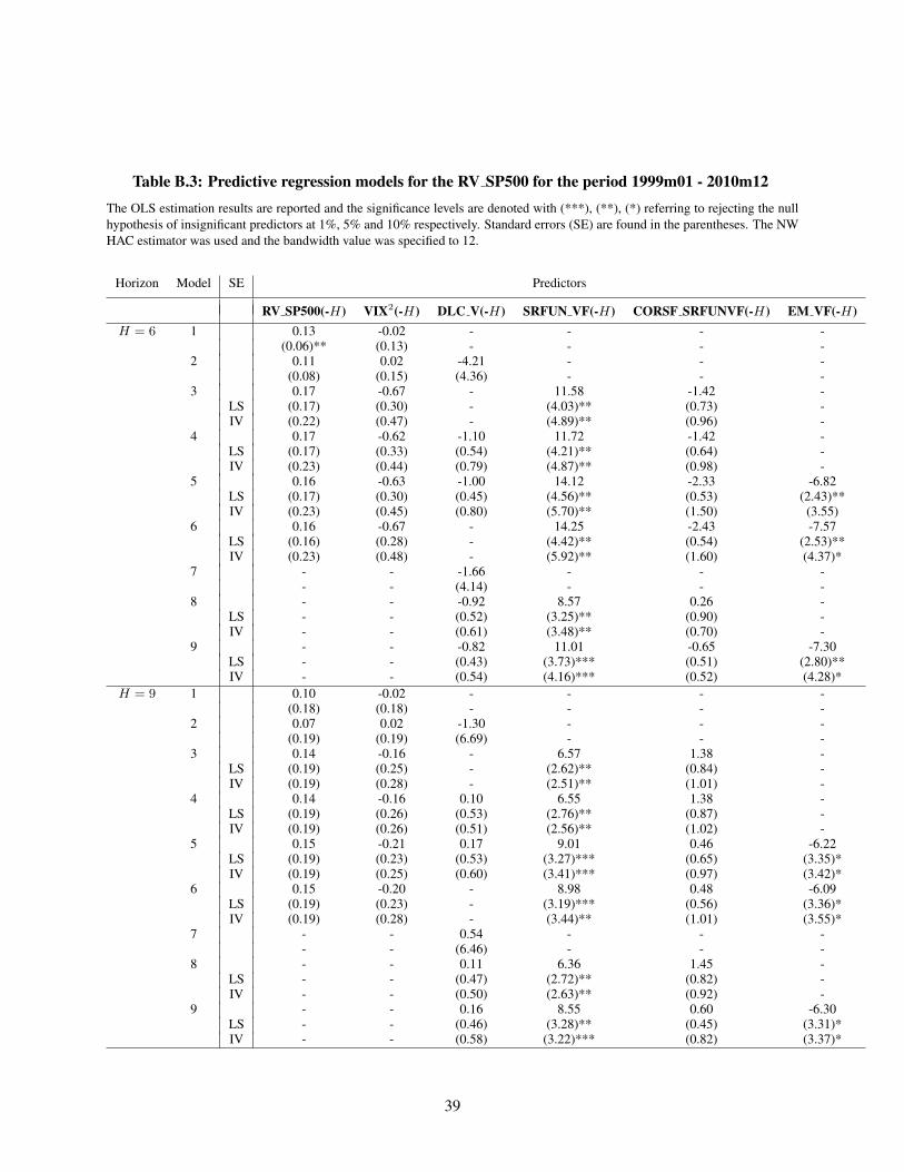
Table B.3: Predictive regression models for the RV SP500 for the period 1999m01 - 2010m12The OLS estimation results are reported and the significance levels are denoted with (***), (**), (*) referring to rejecting the nullhypothesis of insignificant predictors at 1%, 5% and 10% respectively. Standard errors (SE) are found in the parentheses. The NWHAC estimator was used and the bandwidth value was specified to 12.

Horizon Model SE Predictors

RV SP500(-H) VIX2(-H) DLC V(-H) SRFUN VF(-H) CORSF SRFUNVF(-H) EM VF(-H)H = 6 1 0.13 -0.02 - - - -

(0.06)** (0.13) - - - -2 0.11 0.02 -4.21 - - -

(0.08) (0.15) (4.36) - - -3 0.17 -0.67 - 11.58 -1.42 -

LS (0.17) (0.30) - (4.03)** (0.73) -IV (0.22) (0.47) - (4.89)** (0.96) -

4 0.17 -0.62 -1.10 11.72 -1.42 -LS (0.17) (0.33) (0.54) (4.21)** (0.64) -IV (0.23) (0.44) (0.79) (4.87)** (0.98) -

5 0.16 -0.63 -1.00 14.12 -2.33 -6.82LS (0.17) (0.30) (0.45) (4.56)** (0.53) (2.43)**IV (0.23) (0.45) (0.80) (5.70)** (1.50) (3.55)

6 0.16 -0.67 - 14.25 -2.43 -7.57LS (0.16) (0.28) - (4.42)** (0.54) (2.53)**IV (0.23) (0.48) - (5.92)** (1.60) (4.37)*

7 - - -1.66 - - -- - (4.14) - - -

8 - - -0.92 8.57 0.26 -LS - - (0.52) (3.25)** (0.90) -IV - - (0.61) (3.48)** (0.70) -

9 - - -0.82 11.01 -0.65 -7.30LS - - (0.43) (3.73)*** (0.51) (2.80)**IV - - (0.54) (4.16)*** (0.52) (4.28)*

H = 9 1 0.10 -0.02 - - - -(0.18) (0.18) - - - -

2 0.07 0.02 -1.30 - - -(0.19) (0.19) (6.69) - - -

3 0.14 -0.16 - 6.57 1.38 -LS (0.19) (0.25) - (2.62)** (0.84) -IV (0.19) (0.28) - (2.51)** (1.01) -

4 0.14 -0.16 0.10 6.55 1.38 -LS (0.19) (0.26) (0.53) (2.76)** (0.87) -IV (0.19) (0.26) (0.51) (2.56)** (1.02) -

5 0.15 -0.21 0.17 9.01 0.46 -6.22LS (0.19) (0.23) (0.53) (3.27)*** (0.65) (3.35)*IV (0.19) (0.25) (0.60) (3.41)*** (0.97) (3.42)*

6 0.15 -0.20 - 8.98 0.48 -6.09LS (0.19) (0.23) - (3.19)*** (0.56) (3.36)*IV (0.19) (0.28) - (3.44)** (1.01) (3.55)*

7 - - 0.54 - - -- - (6.46) - - -

8 - - 0.11 6.36 1.45 -LS - - (0.47) (2.72)** (0.82) -IV - - (0.50) (2.63)** (0.92) -

9 - - 0.16 8.55 0.60 -6.30LS - - (0.46) (3.28)** (0.45) (3.31)*IV - - (0.58) (3.22)*** (0.82) (3.37)*

39

Table B.4: Predictive regression models for the VRP for the period 1999m01 - 2010m12The OLS estimation results are reported and the significance levels are denoted with (***), (**), (*) referring to rejecting the nullhypothesis of insignificant predictors at 1%, 5% and 10% respectively. Standard errors (SE) are found in the parentheses. The NWHAC estimator was used and the bandwidth value was specified to 12.

Horizon Model SE Predictors

VIX2(-H) DLC V(-H) SRFUN VF(-H) CORSF SRFUNVF(-H) EM VF(-H)H = 6 1 0.08 - - - -

(0.05) - - - -2 0.08 0.55 - - -

(0.05) (2.03) - - -3 -0.29 - 4.99 -1.49 -

LS (0.08) - (1.25)*** (0.26) -IV (0.18) - (1.95)** (0.76)* -

4 -0.27 -0.42 5.05 -1.49 -LS (0.08) (0.26) (1.32)*** (0.25) -IV (0.16)* (0.66) (1.97)** (0.77)* -

5 -0.28 -0.37 6.52 -2.05 -4.17LS (0.07) (0.25) (1.39)*** (0.20) (0.88)***IV (0.16)* (0.70) (2.44)*** (1.06)* (1.77)**

6 -0.30 - 6.56 -2.09 -4.44LS (0.07) - (1.34)*** (0.20) (0.91)***IV (0.18) - (2.54)** (1.12)* (2.28)*

7 - 2.04 - - -- (2.29) - - -

8 - -0.32 3.19 -0.49 -LS - (0.22) (0.99)*** (0.38) -IV - (0.42) (1.27)** (0.33) -

9 - -0.25 4.67 -1.05 -4.44LS - (0.21) (1.10)*** (0.26) (0.93)***IV - (0.44) (1.53)*** (0.47)** (2.14)**

H = 9 1 0.07 - - - -(0.04)* - - - -

2 0.07 1.71 - - -(0.04)* (1.54) - - -

3 -0.19 - 3.09 -1.30 -LS (0.06) - (0.81)*** (0.33)* -IV (0.18) - (1.68)* (1.03) -

4 -0.19 -0.20 3.12 -1.31 -LS (0.06) (0.26) (0.86)*** (0.36) -IV (0.16) (0.53) (1.71)* (1.05) -

5 -0.20 -0.17 4.04 -1.65 -2.34LS (0.06) (0.25) (1.07)*** (0.38)* (1.35)IV (0.17) (0.53) (2.24)* (1.27) (2.02)

6 -0.21 - 4.07 -1.67 -2.47LS (0.06) - (1.02)*** (0.36)** (1.39)IV (0.19) - (2.29)* (1.28) (2.30)

7 - 3.19 - - -- (1.59)** - - -

8 - -0.29 1.82 -0.97 -LS - (0.22) (0.64)*** (0.28) -IV - (0.59) (0.97)* (0.77) -

9 -0.27 2.93 -1.40 -3.20LS - (0.20) (0.88)** (0.29) (1.44)IV - (0.57) (1.57)* (1.09) (3.02)

40

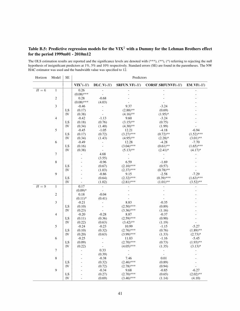
Table B.5: Predictive regression models for the VIX2 with a Dummy for the Lehman Brothers effectfor the period 1999m01 - 2010m12The OLS estimation results are reported and the significance levels are denoted with (***), (**), (*) referring to rejecting the nullhypothesis of insignificant predictors at 1%, 5% and 10% respectively. Standard errors (SE) are found in the parentheses. The NWHAC estimator was used and the bandwidth value was specified to 12.

Horizon Model SE Predictors

VIX2(-H) DLC V(-H) SRFUN VF(-H) CORSF SRFUNVF(-H) EM VF(-H)H = 6 1 0.26 - - - -

(0.08)*** - - - -2 0.28 -0.68 - - -

(0.08)*** (4.03) - - -3 -0.46 - 9.37 -3.24 -

LS (0.17) - (2.88)** (0.69) -IV (0.38) - (4.16)** (1.95)* -

4 -0.42 -1.13 9.60 -3.24 -LS (0.18) (0.76) (3.15)** (0.75) -IV (0.34) (1.40) (4.30)** (1.99) -

5 -0.45 -1.05 12.21 -4.18 -6.94LS (0.17) (0.72) (3.27)*** (0.72)** (1.52)***IV (0.34) (1.43) (4.95)** (2.28)* (3.01)**

6 -0.49 - 12.28 -4.28 -7.70LS (0.16) - (3.04)*** (0.61)** (1.65)***IV (0.38) - (5.13)** (2.41)* (4.17)*

7 - 4.68 - - -- (3.55) - - -

8 - -0.96 6.59 -1.69 -LS - (0.67) (2.10)*** (0.57) -IV - (1.03) (2.37)*** (0.78)** -

9 - -0.86 9.15 -2.58 -7.29LS - (0.64) (2.32)*** (0.39)*** (1.63)***IV - (1.02) (2.81)*** (1.01)** (3.52)**

H = 9 1 0.17 - - - -(0.09)* - - - -

2 0.18 -0.04 - - -(0.11)* (0.41) - - -

3 -0.21 - 8.83 -0.35 -LS (0.10) - (2.50)*** (0.89) -IV (0.23) - (3.36)*** (1.16) -

4 -0.20 -0.28 8.87 -0.37 -LS (0.11) (0.36) (2.59)*** (0.90) -IV (0.22) (0.63) (3.42)** (1.19) -

5 -0.24 -0.23 10.99 -1.15 -5.27LS (0.10) (0.32) (2.76)*** (0.76) (1.89)**IV (0.20) (0.63) (3.99)*** (1.33) (2.73)*

6 -0.25 - 11.03 -1.16 -5.45LS (0.09) - (2.70)*** (0.73) (1.93)**IV (0.22) - (4.05)*** (1.35) (3.13)*

7 - 0.33 - - -- (0.39) - - -

8 - -0.38 7.46 0.01 -LS - (0.32) (2.46)*** (0.89) -IV - (0.72) (2.78)*** (0.94) -

9 - -0.34 9.68 -0.85 -6.27LS - (0.27) (2.70)*** (0.65) (2.02)**IV - (0.69) (3.46)*** (1.14) (4.10)

41

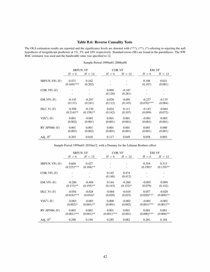
Table B.6: Reverse Causality TestsThe OLS estimation results are reported and the significance levels are denoted with (***), (**), (*) referring to rejecting the nullhypothesis of insignificant predictors at 1%, 5% and 10% respectively. Standard errors (SE) are found in the parentheses. The NWHAC estimator was used and the bandwidth value was specified to 12.

Sample Period 1999m01-2008m08

SRFUN VF COR VF EM VFH = 6 H = 12 H = 6 H = 12 H = 6 H = 12

SRFUN VF(-H) 0.471 0.162 - - 0.108 0.021(0.169)*** (0.202) - - (0.107) (0.081)

COR VF(-H) - - 0.099 -0.187 - -- - (0.120) (0.281) - -

EM VF(-H) -0.145 -0.207 0.028 -0.091 -0.227 -0.135(0.131) (0.241) (0.112) (0.145) (0.070)*** (0.084)

DLC V(-H) -0.509 -0.330 0.024 0.111 -0.143 -0.044(0.214)** (0.159)** (0.142) (0.107) (0.099) (0.072)

VIX2(-H) 0.001 -0.001 0.001 0.001 -0.001 -0.001(0.002) (0.001) (0.001) (0.001) (0.001) (0.001)

RV SP500(-H) 0.001 0.001 0.001 0.001 0.001 0.000(0.002) (0.002) (0.001) (0.001) (0.001) (0.001)

Adj. R2 0.203 0.018 0.117 0.049 0.058 0.003

Sample Period 1999m01-2010m12, with a Dummy for the Lehman Brothers effect

SRFUN VF COR VF EM VFH = 6 H = 12 H = 6 H = 12 H = 6 H = 12

SRFUN VF(-H) 0.604 0.427 - - 0.354 0.313(0.225)*** (0.168)** - - (0.199)* (0.139)**

COR VF(-H) - - 0.145 0.474 - -- - (0.148) (0.412) - -

EM VF(-H) -0.280 -0.404 0.144 -0.260 -0.095 -0.099(0.133)** (0.195)** (0.143) (0.152)* (0.079) (0.142)

DLC V(-H) -0.054 -0.028 -0.004 -0.010 0.057 -0.020(0.018)*** (0.016)* (0.020) (0.025) (0.020)*** (0.009)**

VIX2(-H) -0.003 -0.003 0.000 -0.002 -0.001 -0.002(0.002)* (0.001)** (0.001) (0.002) (0.001)*** (0.001)**

RV SP500(-H) 0.003 0.002 0.001 0.001 0.001 0.001(0.001)*** (0.001)** (0.001)*** (0.001) (0.000)*** (0.000)**

Adj. R2 0.298 0.194 0.285 0.082 0.281 0.184

42

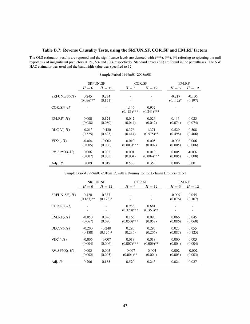
Table B.7: Reverse Causality Tests, using the SRFUN SF, COR SF and EM RF factorsThe OLS estimation results are reported and the significance levels are denoted with (***), (**), (*) referring to rejecting the nullhypothesis of insignificant predictors at 1%, 5% and 10% respectively. Standard errors (SE) are found in the parentheses. The NWHAC estimator was used and the bandwidth value was specified to 12.

Sample Period 1999m01-2008m08

SRFUN SF COR SF EM RFH = 6 H = 12 H = 6 H = 12 H = 6 H = 12

SRFUN SF(-H) 0.245 0.274 - - -0.217 -0.106(0.096)** (0.171) - - (0.112)* (0.197)

COR SF(-H) - - 1.146 0.932 - -- - (0.181)*** (0.241)*** - -

EM RF(-H) 0.000 0.124 0.042 0.026 0.113 0.023(0.088) (0.080) (0.044) (0.042) (0.074) (0.074)

DLC V(-H) -0.213 -0.420 0.376 1.371 0.529 0.508(0.525) (0.623) (0.414) (0.575)** (0.498) (0.406)

VIX2(-H) -0.004 -0.002 0.010 0.005 -0.006 0.006(0.005) (0.006) (0.003)*** (0.007) (0.005) (0.006)

RV SP500(-H) 0.006 0.002 0.001 0.010 0.005 -0.007(0.007) (0.005) (0.004) (0.004)*** (0.005) (0.008)

Adj. R2 0.009 0.019 0.588 0.359 0.006 0.001

Sample Period 1999m01-2010m12, with a Dummy for the Lehman Brothers effect

SRFUN SF COR SF EM RFH = 6 H = 12 H = 6 H = 12 H = 6 H = 12

SRFUN SF(-H) 0.420 0.337 - - -0.009 0.055(0.167)** (0.173)* - - (0.076) (0.107)

COR SF(-H) - - 0.983 0.681 - -- - (0.320)*** (0.353)** - -

EM RF(-H) -0.050 0.096 0.166 0.093 0.066 0.045(0.067) (0.080) (0.050)*** (0.059) (0.086) (0.060)

DLC V(-H) -0.200 -0.248 0.295 0.295 0.023 0.055(0.180) (0.126)* (0.235) (0.206) (0.087) (0.125)

VIX2(-H) -0.006 -0.007 0.019 0.018 0.000 0.003(0.004) (0.006) (0.007)*** (0.009)** (0.004) (0.004)

RV SP500(-H) 0.003 0.003 -0.007 -0.004 0.002 -0.002(0.002) (0.003) (0.004)** (0.004) (0.003) (0.003)

Adj. R2 0.206 0.155 0.520 0.243 0.024 0.027

43