Munich Personal RePEc Archive

What factors affect the export

competitiveness? Malaysian evidence

Amanbayev, Yerkebulan and Masih, Mansur

INCEIF, Malaysia, Business School, Universiti Kuala Lumpur,

Kuala Lumpur, Malaysia

16 April 2017

Online at https://mpra.ub.uni-muenchen.de/102512/

MPRA Paper No. 102512, posted 26 Aug 2020 11:29 UTC

What factors affect the export competitiveness? Malaysian evidence

Yerkebulan Amanbayev 1 and Mansur Masih2

Abstract

Export competitiveness is an important issue for any country. This paper aims to discern the factors

that affect the export competitiveness of a country. Malaysia is taken as a case study. Theoretically,

exports are expected to be affected, among others, by factors such as, inflation rate, interest rate,

exchange rate and money supply. The standard time series techniques are employed for the

analysis. The empirical findings tend to indicate that the most important factor that affects the

export competitiveness is the inflation rate followed by interest rate, exchange rate and money

supply. This is an important finding for the policy makers to bear in mind in order to remain export-

competitive at least in the context of Malaysia.

Keywords: export competitiveness, macro variables, Malaysia

___________________________________

1 INCEIF, Lorong Universiti A, 59100 Kuala Lumpur, Malaysia.

2 Corresponding author, Senior Professor, UniKL Business School, 50300, Kuala Lumpur, Malaysia.

Email: mansurmasih@unikl.edu.my

Introduction

Indeed, the past three decades the Malaysian economy has witnessed rapid economic growth. This

growth has been in conjunction with low inflation, reduced unemployment, diminishing poverty,

reductions in income inequality, and rising per capita income. The manufacturing sector has played

a vital role in Malaysian economic prosperity, contributing substantially to output, employment,

investment and exports. Nonetheless, the export sector has been regarded as the cornerstone in

reinforcing the Malaysian economy, it has also made the country highly dependent on the viability

of the external factors.

In fact, the concept of competitiveness is interrelated to international trade and comparative

advantage. The comparative advantage within international trade theory was first coined by David

Ricardo in 1817. He presented the Ricardian model to describe the patterns of international trade

in “On the Principles of Political Economy and Taxation”. The basic idea of Ricardian model is

that countries will gain from international trade if each country produces and exports the goods in

which they have comparative advantage. It is therefore not necessary for a country to possess

absolute advantage in producing goods, i.e. to be able to produce goods with fewer inputs than any

other country, to benefit from trade. In a nutshell, according to Ricardian model, a country that has

higher labor productivity than other countries in producing goods has a lower price for that goods

and therefore has comparative advantage in producing it.

(1) Objective and Motivation of Research

The competitiveness is an intricate term widely used in both economic research and public debate.

It is therefore necessary to define and clarify the meaning of competitiveness. Despite the wide

use of the concept, there is a consensus that competitiveness can be analyzed on three different

grounds. Firstly, competitiveness can be observed on the macroeconomic level, where nations

competitiveness is studied. Secondly, it is present on the mesoeconomic level, where the

competitiveness of industries and sectors, like E&E sector, is studied. Thirdly competitiveness is

observed on the microeconomic level, where the competitiveness of firms is examined.

Although there are diverse ideas of how competitiveness can be observed on the three levels, the

concept of comparative advantage can be linked to all the three levels of observation. On the

macroeconomic level, competitiveness can be observed as economic growth, as other macro-

indicators, or as comparative advantage due to price differences. Competitiveness on the

mesoeconomic level is observed as the comparative advantage of an industry of a country, and

also as the ability of an industry to gain and maintain a share of domestic and export markets.

Finally, there are several ways of studying competitiveness at the microeconomic level. These are

the firm’s cost efficiency, the quality of its products, ability to meet demand, ability to produce on

large scale and the possession of comparative advantage in production.

Two important differences between comparative advantage and competitiveness are worth to be

mentioned. Firstly, competitiveness can be affected by changes in macroeconomic variables,

whereas comparative advantage is structural in nature. Secondly government support and

protection affect competitiveness, but not comparative advantage. Moreover, Vollrath (1989)

notes that government intervention and competitiveness can change due to exchange rate

fluctuations or regulated prices, but comparative advantage is still unaffected since it is based on

factor endowments or on other non-macroeconomic variables, depending on the underlying theory.

The fact that competitiveness is more sensitive to macroeconomic changes and government

policies shows that comparative advantage denotes a kind of underlying factor of competitiveness,

which is more important , but also harder to observe.

According to Global Competitiveness Report (WEF 2009), there are three factors which bolster

the export competitiveness:

1) Demand-side factors:

- Growing demand for final products that drives higher demand for intermediate products

- Changes in consumer tastes and preferences

- New standards or quality requirements

- Consumer concerns, such as the environment, fair trade, and labor protections

- Marketing practices

- Channels of distribution

2) Supply-side factors:

- Production costs (such as purchased inputs, labor, and capital costs)

- Labor productivity

- Investment

- Capacity utilization

- Infrastructure

- Proximity to the market

- Product innovation and entrepreneurial ability

- Industry structure (such as concentration or vertical and horizontal integration)

3) Exchange rate factors:

- Exchange rate volatility increases risk from exporting and may deter producers from entering the

export market. It may also induce buyers to switch sources of supply.

- An increase in a country’s real exchange rate, observed in changes in the relationship between

domestic and foreign prices for the same goods, means that its exports may become more

expensive than competing products in foreign markets.

The aforementioned are deemed as the external factors which have an impact on the export.

However, there are macroeconomic variables which have direct and indirect influence on the

export competitiveness. The most classical example is the transmission mechanism of exchange

rate on the net exports. This channel involves the interest rate, because when domestic real interest

rates fall due to money supply, domestic currency deposits become less attractive relative to

deposits denominated in foreign currencies. As a result, the value of domestic currency deposits

relative to other currency deposits falls, and its depreciates. The lower value of the domestic

currency makes domestic goods cheaper than foreign goods, thereby causing a rise in net exports.

However, there is an opposite view pertaining to supply-side channels that complicate the effects

of currency depreciation on economic performance. As we know that devaluation makes imported

goods expensive. Therefore, it could have an indirect supply effect on domestic prices. Hence, the

higher cost of imported inputs associated with an exchange rate depreciation increases marginal

cost and leads to higher prices of domestically produced goods (Hyder and Shah,2004). Further,

import-competing firms might increase prices in response to the surge of in foreign competitor

price in order to improve profit margins.

On the other hand, inflation has a correlation with export. For instance, if inflation in the UK is

relatively lower than elsewhere, then UK exports will become more competitive and there will be

an increase in demand for Pound Sterling to buy UK goods. Also foreign goods will be less

competitive and so UK citizens will buy less imports.

Therefore countries with lower inflation rates tend to see an appreciation in the value of their

currency. Conversely, increases in domestic inflation lead to higher prices for exported goods and

a decrease in exports as foreign consumers substitute in favor of lower-priced alternatives

produced within their own country or imported from elsewhere. Substitution occurs in the home

market as well. As the prices of domestically produced goods increase, import prices remain

constant and shoppers shift their preference toward imports, which have fallen in price relative to

inflating domestically produced goods. The net result for a country with a rise in inflation is

decreased exports and increased consumption of imports. The result is a fall in net export.

Generally, a nation running a relatively high rate of inflation will find its currency declining in

value relative to the currencies of countries with lower inflation rates. This relationship is famously

known as purchasing power parity.

Moreover, there is a relationship between interest rate and export. For example, when interest rates

rise in Malaysia (with the price level fixed), Malaysian ringgit bank deposits become more

attractive relative to deposits denominated in foreign currencies, thereby causing a rise in the value

of ringgit deposits relative to other currency deposits, and thus a rise in the exchange rate. The

higher value of the ringgit resulting from the rise in interest rates makes domestic goods more

expensive than foreign goods, thereby causing a fall in net exports.

As we have seen that there are complex and various relationship among the interest rate, money

supply, exchange rate and export. From the aforesaid, we cannot reveal what factor has a strong

effect on the export. Therefore, the main objective and motivation of this paper to find out the

most significant component that impacts on the export competitiveness. The main difference of

this paper from previous, that it aspires to investigate the export competitiveness of Malaysia

from domestic macroeconomic variables, not from the particular sector or industry. Moreover,

there is no paper which addresses this particular issue and dedicated solely to Malaysia.

(2) Literature review

Meanwhile, researchers have conducted surveys on the export competition in different

perspectives. For example, study on electric and electronical export performance and competitive

advantage (Amir, 2000; Fatimah and Alias, 1997; Wilson and Wong, 2000;), competitiveness of

commodity market (e.g Md. Nasir, Mohd Ghazali and Fatimah, 1993; Fatimah and Roslan, 1988;

Muhammad and Habibah, 1993; Muhammad and Abdul Aziz ;1991) and export competitiveness

of ASEAN country with the emergence of China (e.g. Chandran, Veera and Karunagaram 2004;

Chen, Xu and Duan, 2000) and China competitive threat to ASEAN and other exporters (Mukriz

and Nor Aznin, 2005).

Currently, there is no study attempted to use domestic variables pertaining to Malaysian export

competitiveness. However, there are couple of papers which are related to this subject. For

instance, Gulfason (IMF Working paper,1997) tries to identify main export determinants and

economic growth in cross-sectional data which cover 160 countries. He concludes that high

inflation tend to be associated with low exports in proportion to GDP. On the other hand, Irving

B. Kravis and Robert E. Lipsey (National Bureau of Economic Research,1977) carried out the

relationship between export and domestic prices under inflation and exchange rate movements. In

a nutshell, they come up with the following:

- Export price movements differ from those of domestic prices for substantial periods;

- Changes in export/domestic price ratios offset, to some degree, changes in exchange rates and in

relative domestic prices;

- Export/domestic price ratios respond to foreign prices and exchange rates;

- Both export and domestic prices respond to changes in foreign prices and exchange rates, but the

export price response is greater;

- Changes in the export/domestic price ratio are associated with shifts between exporting and

selling at home

M.F.J. Prachowny (Queen’s Economics Department Working Paper,1970) analyses the relation

between inflation and export prices. He points out the possibility that aggregate export prices rise

more slowly than GNP prices if the inflation cost-push or domestic demand-pull, with opposite

results for foreign demand-pull inflation.

Moreover, F.Mishkin (2004), A.Shapiro (2002), R.E. Hall and J.B. Taylor (1988) elaborated the

relationship between interest rate and exports. Basically, it states that increasing interest rates tend

to strengthen the currency of the country, since it is more appealing for foreign investors to buy

that currency and invest them in that country. Thus, if a country’s interest rate is high compared

to foreign interest rates, capital will flow from foreign countries to this country. Such flows could

be enormous if all other factors stay the same. To prevent this, the exchange rate must be

strengthened as a result of the higher demand of the currency. This is called appreciation of the

currency. A higher exchange rate enhances imports since foreign goods get cheaper in comparison

with goods produced domestically. At the same time it reduces exports, since it makes the goods

from that country more expensive to foreigners. Net export is exports minus imports. As a result

of decreasing exports and increasing imports, net exports decline. Another effect of this is that the

inflation is reduced through lower prices for imported goods.

Eventually, there are some papers regarding the relationship between real exchange rate and

inflation, which are explicitly concluded that exchange rate devaluation is a major factor for the

soaring inflation (Kamin 1996 for Mexico; Dornbusch 1990 for Argentina, Brazil, Peru). However,

the others do not find significant impact of devaluation on inflation (Dornbusch 1990 for Bolivia;

Kamas 1995 for Columbia).

(3) Research Methodology, Results and Interpretation

The data series we use in this study are time series data. Empirical work based on time series data

assumes that the underlying time series is stationary (Gujarati, 2003). But many studies have

shown that majority of time series variables are non stationary or integrated of order 1 (Engle and

Granger, 1987). Using non stationary time series in a regression analysis may result in spurious

regression which was firstly pointed out by Granger (1974).

Moreover, in traditional regression, the exogeneity and endogeneity of variables is pre-determined

by the researcher, typically based on the assumption of underlying theory. However, in our case,

as we are dealing with various macroeconomic variables, there is complex relations between them,

and thus no single well established theory. The main superiority of cointegration technique that it

refutes the regression analysis approach whether variable endogenous or exogenous. In fact, we

let the data to determine which variable is leader or follower. In a nutshell, in regression causality

is assumed, whilst in cointegration, it is empirically vindicated with the data.

The data employed in this paper are monthly, which incorporate inflation, export, money supply,

interest rate, nominal exchange rate and dummies of Malaysia. It contains 201 observations

starting from January, 15, 1996. The source of data is DataStream.

3.1. Unit root test

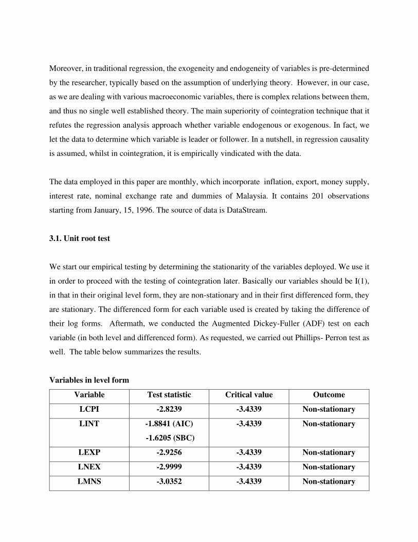
We start our empirical testing by determining the stationarity of the variables deployed. We use it

in order to proceed with the testing of cointegration later. Basically our variables should be I(1),

in that in their original level form, they are non-stationary and in their first differenced form, they

are stationary. The differenced form for each variable used is created by taking the difference of

their log forms. Aftermath, we conducted the Augmented Dickey-Fuller (ADF) test on each

variable (in both level and differenced form). As requested, we carried out Phillips- Perron test as

well. The table below summarizes the results.

Variables in level form

Variable Test statistic Critical value Outcome

LCPI -2.8239 -3.4339 Non-stationary

LINT -1.8841 (AIC)

-1.6205 (SBC)

-3.4339 Non-stationary

LEXP -2.9256 -3.4339 Non-stationary

LNEX -2.9999 -3.4339 Non-stationary

LMNS -3.0352 -3.4339 Non-stationary

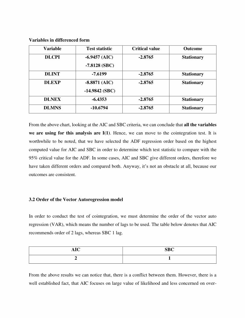
Variables in differenced form

Variable Test statistic Critical value Outcome

DLCPI -6.9457 (AIC)

-7.8128 (SBC)

-2.8765 Stationary

DLINT -7.6199 -2.8765 Stationary

DLEXP -8.8871 (AIC)

-14.9842 (SBC)

-2.8765 Stationary

DLNEX -6.4353 -2.8765 Stationary

DLMNS -10.6794 -2.8765 Stationary

From the above chart, looking at the AIC and SBC criteria, we can conclude that all the variables

we are using for this analysis are I(1). Hence, we can move to the cointegration test. It is

worthwhile to be noted, that we have selected the ADF regression order based on the highest

computed value for AIC and SBC in order to determine which test statistic to compare with the

95% critical value for the ADF. In some cases, AIC and SBC give different orders, therefore we

have taken different orders and compared both. Anyway, it’s not an obstacle at all, because our

outcomes are consistent.

3.2 Order of the Vector Autoregression model

In order to conduct the test of cointegration, we must determine the order of the vector auto

regression (VAR), which means the number of lags to be used. The table below denotes that AIC

recommends order of 2 lags, whereas SBC 1 lag.

AIC SBC

2 1

From the above results we can notice that, there is a conflict between them. However, there is a

well established fact, that AIC focuses on large value of likelihood and less concerned on over-

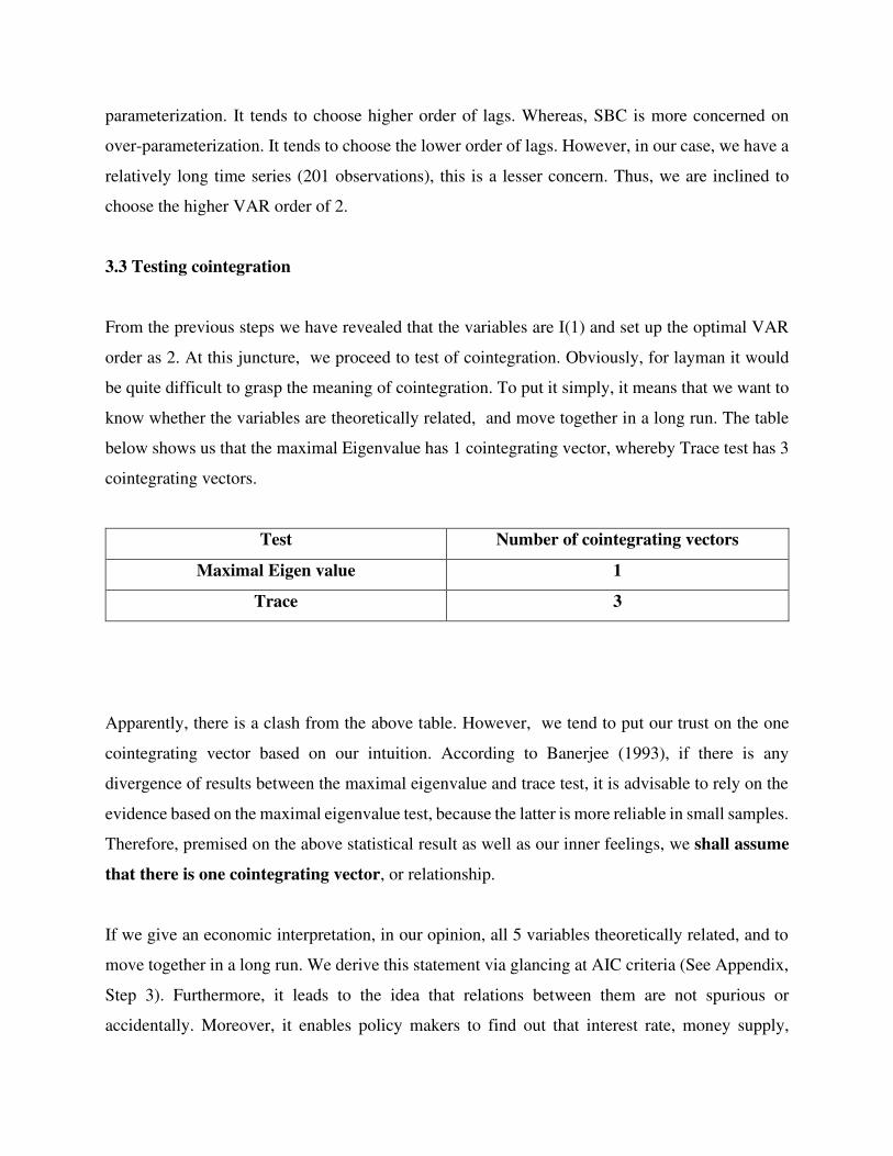
parameterization. It tends to choose higher order of lags. Whereas, SBC is more concerned on

over-parameterization. It tends to choose the lower order of lags. However, in our case, we have a

relatively long time series (201 observations), this is a lesser concern. Thus, we are inclined to

choose the higher VAR order of 2.

3.3 Testing cointegration

From the previous steps we have revealed that the variables are I(1) and set up the optimal VAR

order as 2. At this juncture, we proceed to test of cointegration. Obviously, for layman it would

be quite difficult to grasp the meaning of cointegration. To put it simply, it means that we want to

know whether the variables are theoretically related, and move together in a long run. The table

below shows us that the maximal Eigenvalue has 1 cointegrating vector, whereby Trace test has 3

cointegrating vectors.

Test Number of cointegrating vectors

Maximal Eigen value 1

Trace 3

Apparently, there is a clash from the above table. However, we tend to put our trust on the one

cointegrating vector based on our intuition. According to Banerjee (1993), if there is any

divergence of results between the maximal eigenvalue and trace test, it is advisable to rely on the

evidence based on the maximal eigenvalue test, because the latter is more reliable in small samples.

Therefore, premised on the above statistical result as well as our inner feelings, we shall assume

that there is one cointegrating vector, or relationship.

If we give an economic interpretation, in our opinion, all 5 variables theoretically related, and to

move together in a long run. We derive this statement via glancing at AIC criteria (See Appendix,

Step 3). Furthermore, it leads to the idea that relations between them are not spurious or

accidentally. Moreover, it enables policy makers to find out that interest rate, money supply,

export, exchange rate and inflation are intertwined and interrelated in the long term, and hence

they should monitor them properly and implement prudent policy and decision-making. We would

like to point out as well, that there are various economic theories that underpin relations between

those variables. For instance, Purchasing power parity which stems from the exchange rate and

inflation, the Fisher effect which deals with the inflation and interest rate and transmission

mechanism of money supply to interest rate.

Although, cointegration tells us the existence of the long-run theoretical relationship, however, it

does not provide which of the above variables is the leading one (exogenous) and which one is the

lagging (endogenous). Thus cointegration cannot show the causation among the variables. This

problem will be solved in subsequent steps.

3.4 Long run structuring model

It is worth to be noted that, before the advent of LRSM, one of the main limitations of time-series

was the fact that time series was mainly atheoretical and it was disparaged by the proponents of

the conventional regression analysis for this flaw. However, with the revelation of the LRSM, the

robust answer was found, that is LRSM proves theoretical relationship between the cointegrated

variables. It does so by imposing on the variables’ long-run relations identifying and over-

identifying restrictions based on economic theory. Hence, time-series technique unified the data

and theory through the application of LRSM, and thus we could test obtained coefficients vis-à-

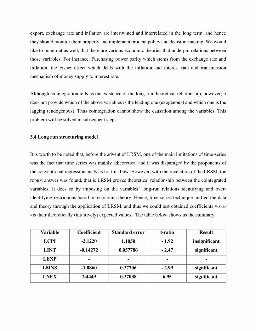
vis their theoretically (intuitively) expected values. The table below shows us the summary:

Variable Coefficient Standard error t-ratio Result

LCPI -2.1220 1.1050 - 1.92 insignificant

LINT -0.14272 0.057786 - 2.47 significant

LEXP - - - -

LMNS -1.0860 0.37706 - 2.99 significant

LNEX 2.4449 0.37038 6.95 significant

As we see from the results, LINT, LMNS, LNEX are significant, except LCPI. Therefore, we were

curious to find out, why LCPI is insignificant. Hence, we decided to scrutinize the significance of

the variables by subjecting the estimates to over-identifying restrictions. We run it for all variables,

and LCPI turn out to significant level as well as other variables. We would like to clarify, that we

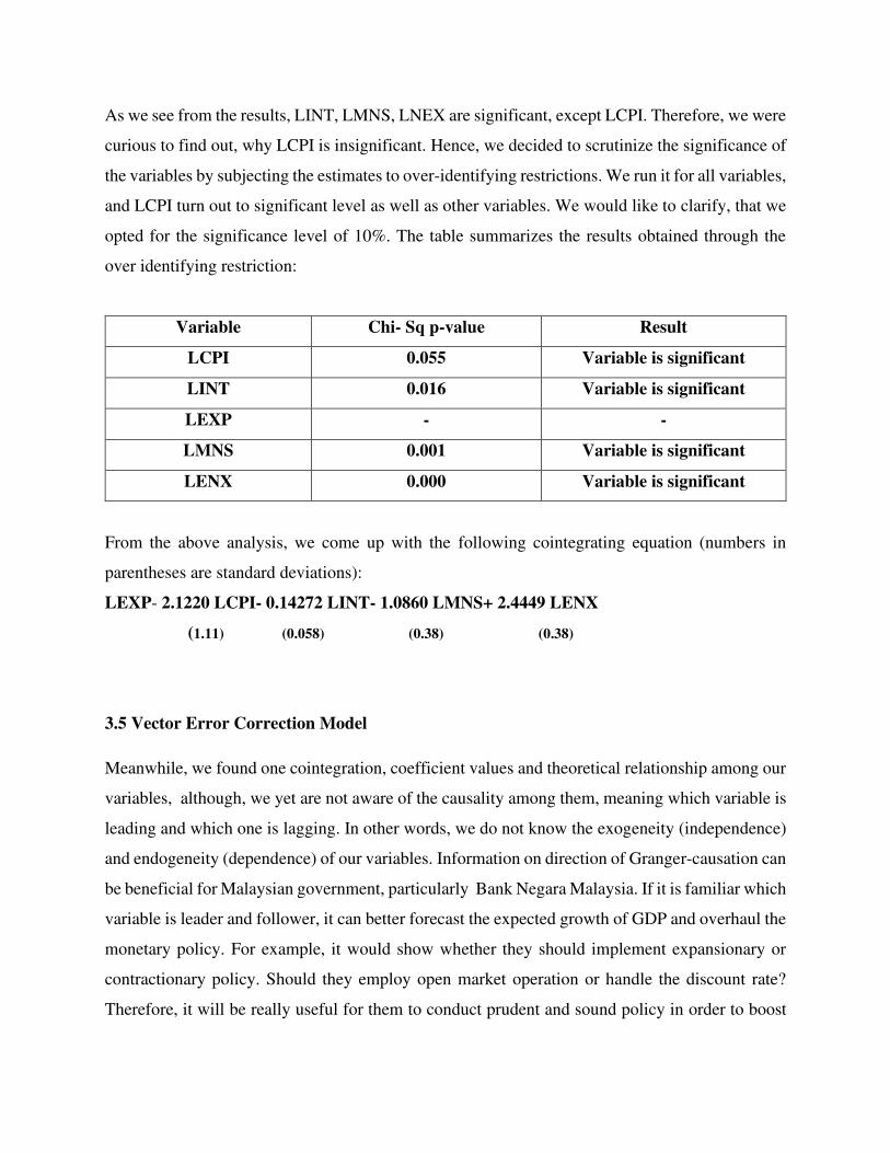
opted for the significance level of 10%. The table summarizes the results obtained through the

over identifying restriction:

Variable Chi- Sq p-value Result

LCPI 0.055 Variable is significant

LINT 0.016 Variable is significant

LEXP - -

LMNS 0.001 Variable is significant

LENX 0.000 Variable is significant

From the above analysis, we come up with the following cointegrating equation (numbers in

parentheses are standard deviations):

LEXP- 2.1220 LCPI- 0.14272 LINT- 1.0860 LMNS+ 2.4449 LENX

(1.11) (0.058) (0.38) (0.38)

3.5 Vector Error Correction Model

Meanwhile, we found one cointegration, coefficient values and theoretical relationship among our

variables, although, we yet are not aware of the causality among them, meaning which variable is

leading and which one is lagging. In other words, we do not know the exogeneity (independence)

and endogeneity (dependence) of our variables. Information on direction of Granger-causation can

be beneficial for Malaysian government, particularly Bank Negara Malaysia. If it is familiar which

variable is leader and follower, it can better forecast the expected growth of GDP and overhaul the

monetary policy. For example, it would show whether they should implement expansionary or

contractionary policy. Should they employ open market operation or handle the discount rate?

Therefore, it will be really useful for them to conduct prudent and sound policy in order to boost

the growth of the economy. Hence, the exogenous variable would be the proxy for the policy

makers.

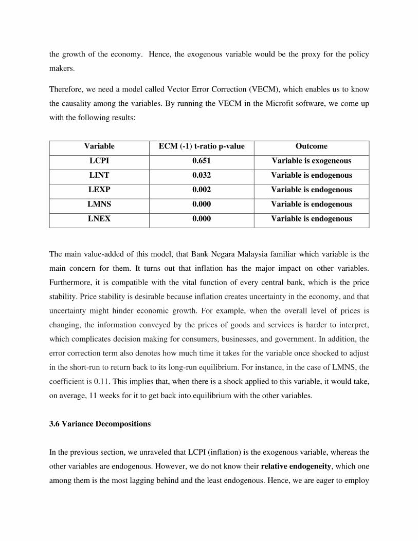
Therefore, we need a model called Vector Error Correction (VECM), which enables us to know

the causality among the variables. By running the VECM in the Microfit software, we come up

with the following results:

Variable ECM (-1) t-ratio p-value Outcome

LCPI 0.651 Variable is exogeneous

LINT 0.032 Variable is endogenous

LEXP 0.002 Variable is endogenous

LMNS 0.000 Variable is endogenous

LNEX 0.000 Variable is endogenous

The main value-added of this model, that Bank Negara Malaysia familiar which variable is the

main concern for them. It turns out that inflation has the major impact on other variables.

Furthermore, it is compatible with the vital function of every central bank, which is the price

stability. Price stability is desirable because inflation creates uncertainty in the economy, and that

uncertainty might hinder economic growth. For example, when the overall level of prices is

changing, the information conveyed by the prices of goods and services is harder to interpret,

which complicates decision making for consumers, businesses, and government. In addition, the

error correction term also denotes how much time it takes for the variable once shocked to adjust

in the short-run to return back to its long-run equilibrium. For instance, in the case of LMNS, the

coefficient is 0.11. This implies that, when there is a shock applied to this variable, it would take,

on average, 11 weeks for it to get back into equilibrium with the other variables.

3.6 Variance Decompositions

In the previous section, we unraveled that LCPI (inflation) is the exogenous variable, whereas the

other variables are endogenous. However, we do not know their relative endogeneity, which one

among them is the most lagging behind and the least endogenous. Hence, we are eager to employ

Variance Decomposition (VDC) technique. VDC indicates how much each variable contributes to

the other variables in a model. In other words, VDC decomposes variance of forecast error of a

particular variable into proportions attributable to shocks from each variable in system including

its own. Therefore, fluctuations of the variable explained mostly by its own past movements is the

least dependent on the others. There are two types of the VDC analysis: orthogonalized and

generalized. In orthogonalized VDC partitions of the forecast error variance attributed to other

variables in the model add up to 100%, while it is not applied in the generalized form. In addition,

orthogonalized VDC depends on a particular ordering of the variables, that is the first variable in

the list would be considered as the most exogenous, thus orthogonalized form of VDC could give

biased results, while generalized does not have such restriction. Finally, in contrast to generalized

form, orthogonalized form assumes that when one of the variables is shocked other variables are

kept constant, that is they do not vary over time or switched off. Therefore, we deploy the

generalized form of VDC. However, the orthogonalized VDC results are also provided.

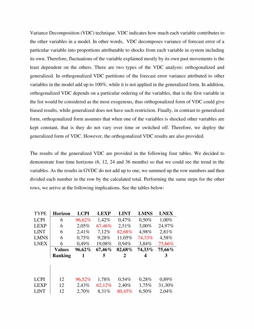
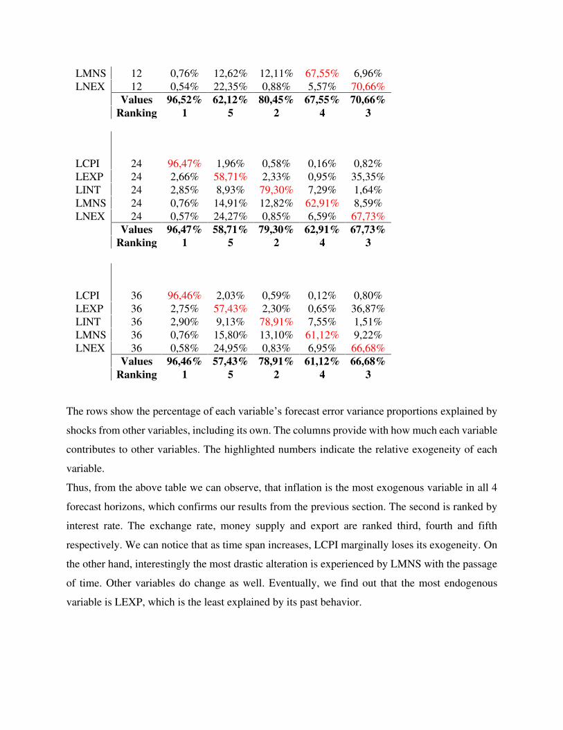
The results of the generalized VDC are provided in the following four tables. We decided to

demonstrate four time horizons (6, 12, 24 and 36 months) so that we could see the trend in the

variables. As the results in GVDC do not add up to one, we summed up the row numbers and then

divided each number in the row by the calculated total. Performing the same steps for the other

rows, we arrive at the following implications. See the tables below:

TYPE Horizon LCPI LEXP LINT LMNS LNEX

LCPI 6 96,62% 1,42% 0,47% 0,50% 1,00%

LEXP 6 2,05% 67,46% 2,51% 3,00% 24,97%

LINT 6 2,41% 7,12% 82,68% 4,98% 2,81%

LMNS 6 0,75% 9,28% 11,05% 74,33% 4,58%

LNEX 6 0,49% 19,08% 0,94% 3,84% 75,66%

Values 96,62% 67,46% 82,68% 74,33% 75,66%

Ranking 1 5 2 4 3

LCPI 12 96,52% 1,78% 0,54% 0,28% 0,89%

LEXP 12 2,43% 62,12% 2,40% 1,75% 31,30%

LINT 12 2,70% 8,31% 80,45% 6,50% 2,04%

LMNS 12 0,76% 12,62% 12,11% 67,55% 6,96%

LNEX 12 0,54% 22,35% 0,88% 5,57% 70,66%

Values 96,52% 62,12% 80,45% 67,55% 70,66%

Ranking 1 5 2 4 3

LCPI 24 96,47% 1,96% 0,58% 0,16% 0,82%

LEXP 24 2,66% 58,71% 2,33% 0,95% 35,35%

LINT 24 2,85% 8,93% 79,30% 7,29% 1,64%

LMNS 24 0,76% 14,91% 12,82% 62,91% 8,59%

LNEX 24 0,57% 24,27% 0,85% 6,59% 67,73%

Values 96,47% 58,71% 79,30% 62,91% 67,73%

Ranking 1 5 2 4 3

LCPI 36 96,46% 2,03% 0,59% 0,12% 0,80%

LEXP 36 2,75% 57,43% 2,30% 0,65% 36,87%

LINT 36 2,90% 9,13% 78,91% 7,55% 1,51%

LMNS 36 0,76% 15,80% 13,10% 61,12% 9,22%

LNEX 36 0,58% 24,95% 0,83% 6,95% 66,68%

Values 96,46% 57,43% 78,91% 61,12% 66,68%

Ranking 1 5 2 4 3

The rows show the percentage of each variable’s forecast error variance proportions explained by

shocks from other variables, including its own. The columns provide with how much each variable

contributes to other variables. The highlighted numbers indicate the relative exogeneity of each

variable.

Thus, from the above table we can observe, that inflation is the most exogenous variable in all 4

forecast horizons, which confirms our results from the previous section. The second is ranked by

interest rate. The exchange rate, money supply and export are ranked third, fourth and fifth

respectively. We can notice that as time span increases, LCPI marginally loses its exogeneity. On

the other hand, interestingly the most drastic alteration is experienced by LMNS with the passage

of time. Other variables do change as well. Eventually, we find out that the most endogenous

variable is LEXP, which is the least explained by its past behavior.

Moreover, the above results compel Bank Negara Malaysia to revise the inflation rate rigorously.

It implies that it should handle and maintain inflation rate in a decent manner in order to bolster

the growth of the overall economy. It might be suggested for them to set up a robust inflation

targeting in order to equalize various conflicting goals of monetary policy. They should be aware,

that controlling price stability may trigger the rise or fall of export competitiveness of Malaysia.

3.7 Impulse response function

The impulse response function presents the same information as in the VDC, but in a graphical

form. The IRFs also show how much time it would require for the variables to get back to their

long-run equilibrium in case of a variable-specific shock.

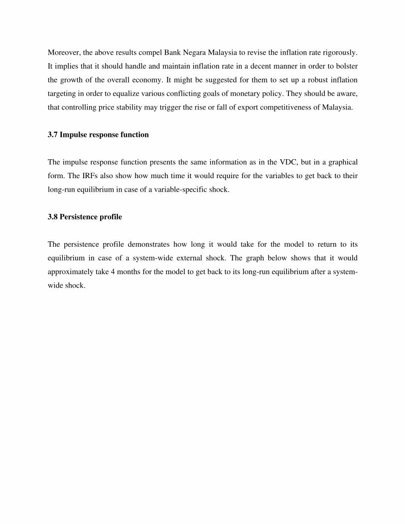
3.8 Persistence profile

The persistence profile demonstrates how long it would take for the model to return to its

equilibrium in case of a system-wide external shock. The graph below shows that it would

approximately take 4 months for the model to get back to its long-run equilibrium after a system-

wide shock.

(4) Conclusion and policy implication

This paper attempted to address the issue of export competitiveness of Malaysia by using

macroeconomic factors. The study shows that the most affecting factor on export is inflation. From

the purchasing power parity, we know that inflation has an impact on the export indirectly. It

involves the exchange rate in the middle, which implies that the country running high rate of

inflation will find its currency depreciating in value relative to the currencies of countries with

lower inflation rates.

Inflation has adverse ramifications for the overall economy, such as it erodes living standards,

affects distribution of income, rising inflationary expectations can lead to upward spiraling

inflation and damages international competitiveness. Therefore, Bank Negara Malaysia in

coordination with the government should find a clue how to control inflation rate in a proper

manner and at the same time to bolster the growth of export. As it was mentioned, they may adopt

inflation targeting model which is aimed to steer actual inflation towards the target through the use

of interest rate changes and other monetary tools. This precedent has been successfully

implemented in some countries. As Variance Decomposition model indicates, that an interest rate

Persistence Profile of the effect of a system-wide shock to CV'(s)

CV1

Horizon

0.0

0.2

0.4

0.6

0.8

1.0

0 2 4 6 8 10 12 14 16 18 20 22 24 26 28 30 32 34 36 38 40 42 44 46 48 50 50

is ranked as the second significant factor which affects export. Therefore, they should supervise

the overnight policy rate carefully in order to prevent currency appreciation, which leads to the fall

of net export. Finally, Bank Negara Malaysia has to uphold ringgit via the foreign exchange market

intervention, because exchange rate has a transmission mechanism through to inflation which is

well known as exchange rate pass-through model.

In the end, it is worthwhile to be mentioned, that current study has limitations and hence

shortcomings. For instance, other macroeconomic variables, namely GDP, import etc. can be taken

into account, and thus could give different results. In addition, particular sector could be deployed

to find its correlation with inflation. Moreover, according to Bank Negara Malaysia, the inflation

rate was 3.2% which indicates it run low inflation already. Therefore, there might be other essential

factors that have an influence on the export. Nevertheless, due diligence and effort should be

employed to achieve this goal.

References

Amir, M. (2000) Trade Liberalisation and Malaysian Export Competitiveness: Prospects,

Problems and Policy Implication, Conference on International Trade Education and Research,

Melbourne.

Banerjee, A. (1993) ,Cointegration, Error Correction and the Econometric Analysis of Non-

Stationary Data, New York, Oxford University Press.

Chen, K.Z., Xu, T. and Duan Y., (2000); Competitive of Canadian Agri-food Export against

competitors in Asia:1980-97; Journal of International Food and Agribusiness Marketing, 11(4), 1

-19

Dornbusch, R. (1990), Extreme inflation: dynamics and stabilization, Brooking Papers on

economic activity, 2, 1 – 84.

Engle, R.F. and C.W. Granger (1987), Cointegration and Error Correction Representation,

Estimation and Testing, Econometrica, 55, 251-276.

Global Competitiveness Report (2009), World Economic Forum, Geneva, Switzerland.

Granger, C. and Newbold, P. (1974). Spurious Regression in Econometrics. Journal of

Econometrics, 2, 111-120

Gujarati, D.N. (2003) Basic Econometrics, West Point, US Military Academy, New York,

McGraw Hill

Gulfaso, T., Exports, Inflation and Growth, IMF Working paper,1997

Hall, R.E. and Taylor, J. B.(1988) Macroeconomics. Theory, Performance, and Policy, 2nd

Edition:, New York, Norton International Student Edition.

Hyder, Z. and Shah S, (2004), Exchange rate pass-through to domestic price in Pakistan, Working

Paper No 5, State bank of Pakistan.

Kamas, L. (1995), Monetary policy and inflation under the crawling peg, Journal of Development

Economics, 46, 145-161

Kamin, S..B.(1996), Exchange rates and inflation in exchange rate based stabilizations: an

empirical examination, International Finance Discussion Paper 154

Kravis, I. B. and Lipsey, R. E.(1971), Price Competitiveness in World Trade, NBER.

Mishkin, F. S. (2010). The Economics of Money, Banking, and Financial Markets,. Colombia

University, New York, Pearson.

Mohamad, H. A., Fatimah, M. A. and Abdul Aziz, A. R. (1992) Market share analysis of

Malaysia’s Palm Oil Exports: Implication on its Competitiveness, Journal of Economic Malaysia,

26, 3-20.

Mohamad, H. A. and Habibah, S., (1993); Constant Market Share Analysis: An Application to NR

Export of Major Producing Countries; Journal of NR research, 8(1); 68-78.

Prachowny, M. F. J.(1970), The relation between inflation and export prices: an aggregate study,

Working Paper No 27, Economics Department, Queen’s University.

Shapiro, A. (2014) Multinational Financial Management, Tenth edition, New York, Wiley.

Wilson, P. and Wong, Y. M. (2000). The export competitiveness of ASEAN economies, 1986-95.

National University of Singapore, Singapore.