What is Population Genetics?

About microevolution (evolution within species)

The study of the change of allele frequencies,

genotype frequencies, and phenotype frequencies

Factors causing genotype frequency changes or evolutionary principles

• Selection = variation in fitness; heritable• Mutation = change in DNA of genes• Migration = movement of genes across populations

– Vectors = Pollen, Spores

• Recombination = exchange of gene segments• Non-random Mating = mating between neighbors

rather than by chance• Random Genetic Drift = if populations are small

enough, by chance, sampling will result in a different allele frequency from one generation to the next.

Pathogen Population Genetics

• must constantly adapt to changing environmental conditions to survive– High genetic diversity = easily adapted– Low genetic diversity = difficult to adapt to changing

environmental conditions– important for determining evolutionary potential of a

pathogen

• If we are to control a disease, must target a population rather than individual

• Exhibit a diverse array of reproductive strategies that impact population biology

Molecular Markers

• DNA & PROTEINS – mtDNA = often used in systematics; in general, no recombination =

uniparental inheritance– cpDNA = often used in systematics; in general, no recombination =

uniparental inheritance– Microsatellites = tandem repeats; genotyping & population structure– Allozymes = variations of proteins; population structure– RAPDs = short segments of arbitrary sequences; genotyping– RFLPs = variants in DNA exposed by cutting with restriction enzymes;

genotyping, population structure– AFLPs = after digest with restriction enzymes, a subset of DNA fragments

are selected for PCR amplification; genotyping

Analytical Techniques

– Hardy-Weinberg Equilibrium • p2 + 2pq + q2 = 1• Departures from non-random mating

– F-Statistics• measures of genetic differentiation in populations

– Genetic Distances – degree of similarity between OTUs • Nei’s• Reynolds• Jaccards• Cavalli-Sforza

– Tree Algorithms – visualization of similarity• UPGMA• Neighbor Joining

Levels of Analyses

Individual

• identifying parents & offspring– very important in zoological circles – identify patterns of mating between individuals (polyandry, etc.)

In fungi, it is important to identify the "individual" -- determining clonal individuals from unique individuals that resulted from a single mating event.

Armillaria gallica “Humongous Fungus”

rhizomorphs

Levels of Analyses cont…

• Families – looking at relatedness within colonies (ants, bees, etc.)

• Population – level of variation within a population. – Dispersal = indirectly estimate by calculating

migration– Conservation & Management = looking for founder

effects (little allelic variation), bottlenecks (reduction in population size leads to little allelic variation)

• Species – variation among species = what are the relationship between species.

• Family, Order, ETC. = higher level phylogenies

Founder Effects

• Establishment of a population by a few individuals can profoundly affect genetic variation– Consequences of Founder effects

• Fewer alleles• Fixed alleles• Modified allele frequencies compared to source pop

– Perhaps due to “new environment”

Potato Blight

• Phytophthora infestans

• great Irish famine of 1845-1849– 1,000,000 died

• Origin of P. infestans – Mexico = highest genetic diversity; likely origin– Ireland = decreased genetic diversity due to founder

effect– Decreased genetic differentiation in other regions

• Europe, North America

Hardy Weinberg Equilibriumand F-Stats

• In general, requires co-dominant marker system

• Codominant = expression of heterozygote phenotypes that differ from either homozygote phenotype.

• AA, Aa, aa

Codominant Molecular Tools– Allozymes = different versions of

proteins.• One of the major first tools for

analyzing population structure

Advantages:InexpensiveEasily Obtained

Disadvantages:

Coding regions = violate assumptions of analytical techniques

Invariable in many fungi = inadequate for looking at variation

– Microsatellites = repetitive sequences in the DNA (e.g. AC)12

• Very popular for analyzing population structure

• Forensic applications

Advantages:Hypervariable

GenotypingPopulation

Structure

Disadvantages:

High cost of Development

Dominant Marker

Allele Frequencies

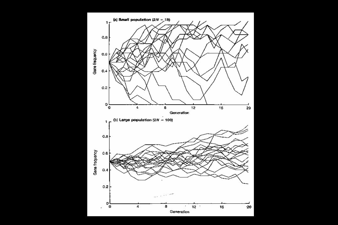
• Allele frequencies (gene frequencies) = proportion of all alleles in an all individuals in the group in question which are a particular type

• Allele frequencies: p + q = 1

• Expected genotype frequencies: p2 + 2pq + q2

Hardy-Weinberg Equilibrium

• Null Model = population is in HW Equilibrium– Useful– Often predicts genotype frequencies well

if only random mating occurs, then allele frequenciesremain unchanged over time.

After one generation of random-mating, genotype frequencies are given by

AA Aa aap2 2pq q2

p = freq (A)q = freq (a)

Hardy-Weinberg Theorem

• The possible range for an allele frequency or genotype frequency therefore lies between ( 0 – 1)• with 0 meaning complete absence of that allele or genotype from the population (no individual in the population carries that allele or genotype)• 1 means complete fixation of the allele or genotype (fixation means that every individual in the population is homozygous for the allele -- i.e., has the same genotype at that locus).

Expected Genotype Frequencies

1) diploid organism2) sexual reproduction3) generations are non-overlapping4) mating occurs at random5) large population size6) migration = 07) mutation = 08) no selection on genes

ASSUMPTIONS

Locus

Sample 1 2 3

1 3,4 2,2 1,1

2 4,4 2,2 1,2

3 4,4 1,2 1,2

4 4,4 2,2 1,1

5 4,4 1,2 1,1

6 1,4 1,2 1,1

7 2,4 2,2 1,1

8 4,4 2,2 1,1

9 2,4 1,2 1,1

10 1,4 2,3 2,2

11 2,4 2,2 2,2

12 2,3 2,2 2,2

13 4,4 1,2 1,1

14 1,4 2,3 1,2

15 4,4 1,2 1,2

16 1,4 1,1 1,1

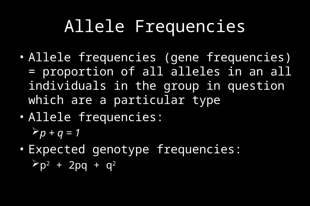
Locus 1Allele 1 = 4/32 = 0.125Allele 2 = 4/32 = 0.125Allele 3 = 2/32 = 0.0625Allele 4 = 22/32 = 0.6875

Allele frequencies = 0.125 + 0.125 + 0.00625 + 0.6875 = 1

Locus 2Allele 1 = 8/32 = 0.2500Allele 2 = 22/32 = 0.6875Allele 3 = 2/32 = 0.0625

Locus 3Allele 1 = 10/32 = 0.3125Allele 2 = 22/32 = 0.6875

EXP OBS (OBS-EXP)2/EXP

LOCUS 1 1,1 (0.1250)2 0.0156 0.0000 0.0156

1,2 (0.125*0.125)*2 0.0313 0.0000 0.0313

1,3 (0.125*0.0625)*2 0.0157 0.0000 0.0157

1,4 (0.125*0.6875)*2 0.1718 0.2500 0.0356

2,2 (0.125)2 0.0156 0.0000 0.0156

2,3 (0.125*0.0625)*2 0.0156 0.0625 0.1410

2,4 (0.125*0.6875)*2 0.1719 0.1875 0.0014

3,3 (0.0625)2 0.0039 0.0000 0.0039

3,4 (0.0625*0.6875)*2 0.0859 0.0625 0.0064

4,4 (0.6875)2 0.4727 0.4375 0.0026

EXP OBS (OBS-EXP)2/EXP

LOCUS 2 1,1 (0.2500)2 0.0625 0.0625 0.0000

1,2 (0.2500*0.6875)*2 0.3438 0.3750 0.0028

1,3 (0.2500*0.0625)*2 0.0313 0.0000 0.0313

2,2 (0.6875)2 0.4727 0.4375 0.0026

2,3 (0.6875*0.0625)*2 0.0859 0.1250 0.0178

3,3 (0.0625)2 0.0038 0.0000 0.0038

LOCUS 3 1,1 (0.3125)2 0.0977 0.5625 2.2112

1,2 (0.3125*0.6875)*2 0.4297 0.2500 0.0752

2,2 (0.6875)2 0.4726 0.1875 0.1720

CHI-SQUARED TEST = 2.7858

P 0.999984

If the only force acting on the population is random mating, allele frequencies remain unchanged and genotypic frequencies are constant.

Mendelian genetics implies that genetic variability can persist indefinitely, unless other evolutionary forces act to remove it

IMPORTANCE OF HW THEOREM

Departures from HW Equilibrium

• Check Gene Diversity = Heterozygosity– If high gene diversity = different genetic sources due

to high levels of migration

• Inbreeding - mating system “leaky” or breaks down allowing mating between siblings

• Asexual reproduction = check for clones– Risk of over emphasizing particular individuals

• Restricted dispersal = local differentiation leads to non-random mating

F Stats

• FIS = (HS – HI)/(HE)

• FST = (HT – HS)/(HT)

• FIT = (HT – HI)/(HT)

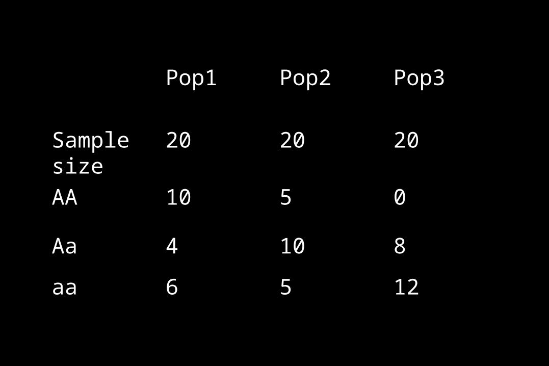
Pop1 Pop2 Pop3

Sample size

20 20 20

AA 10 5 0

Aa 4 10 8

aa 6 5 12

Pop1 Pop2 Pop3

Freq

p (20 + 1/2*8)/40 = 0.60

(10+1/2*20)/40 = .50

(0+1/2*16)/40 = 0.20

q (12 + 1/2*8)/40 = 0.40

(10+1/2*20)/40 = .50

(24+1/2*16)/40 = 0.80

• Calculate HOBS

– Pop1: 4/20 = 0.20– Pop2: 10/20 = 0.50– Pop3: 8/20 = 0.40

• Calculate HEXP (2pq)– Pop1: 2*0.60*0.40 = 0.48– Pop2: 2*0.50*0.50 = 0.50– Pop3: 2*0.20*0.80 = 0.32

• Calculate F = (HEXP – HOBS)/ HEXP

• Pop1 = (0.48 – 0.20)/(0.48) = 0.583• Pop2 = (0.50 – 0.50)/(0.50) = 0.000• Pop3 = (0.32 – 0.40)/(0.32) = -0.250

Local Inbreeding Coefficient

Pop Hs HI p q HT FIS FST FIT

1 0.48 0.20 0.60 0.40

2 0.50 0.50 0.50 0.50

3 0.32 0.40 0.20 0.80

Mean 0.43 0.37 0.43 0.57 0.49 -0.14 0.12 0.24

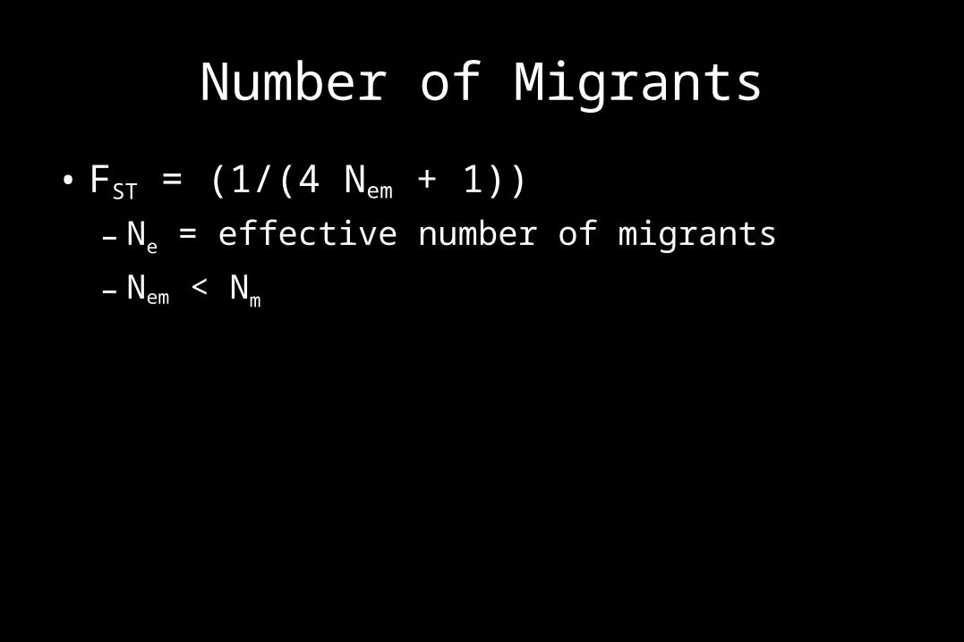
Number of Migrants

• FST = (1/(4 Nem + 1))

– Ne = effective number of migrants

– Nem < Nm

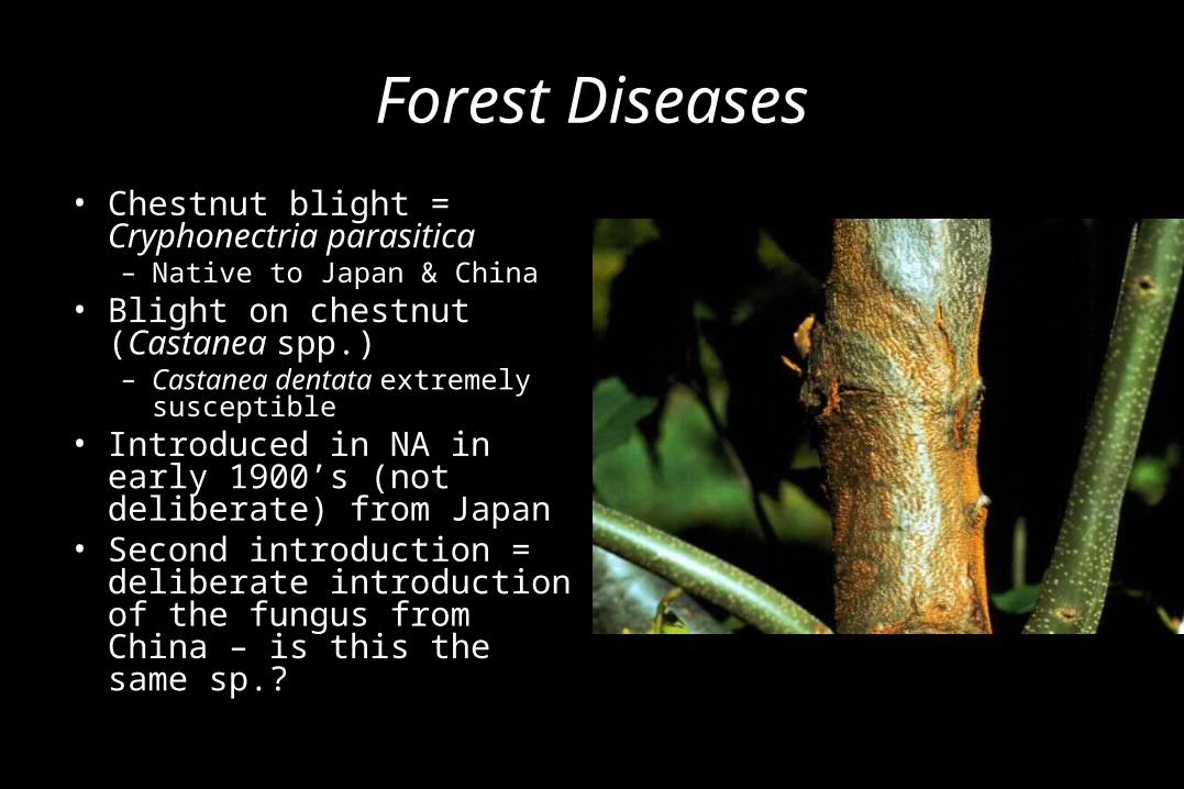
Forest Diseases

• Chestnut blight = Cryphonectria parasitica– Native to Japan & China

• Blight on chestnut (Castanea spp.)– Castanea dentata extremely

susceptible• Introduced in NA in early

1900’s (not deliberate) from Japan

• Second introduction = deliberate introduction of the fungus from China – is this the same sp.?

Cryphonectria parasitica

• Using genetic similarities– Identified probable source population for US introduction as

Japan rather than China– China & Japan are not closely related

• Longer history of independent evolution

– Two clonal populations = no sexual reproduction• Likely founded by clones

– Deviations from HW equilibrium• Unrelated genotypes in populations suggests restricted migration• Genetic drift main force in evolution