What is superresolution microscopy?

John Bechhoefera)

Department of Physics, Simon Fraser University, Burnaby, British Columbia, Canada V5A 1S6

(Received 5 May 2014; accepted 20 October 2014)

In this paper, we discuss what is, what is not, and what is only sort of superresolution microscopy.

We begin by considering optical resolution, first in terms of diffraction theory, then in terms of

linear-systems theory, and finally in terms of techniques that use prior information, nonlinearity,

and other tricks to improve resolution. This discussion reveals two classes of superresolution

microscopy, “pseudo” and “true.” The former improves images up to the diffraction limit, whereas

the latter allows for substantial improvements beyond the diffraction limit. The two classes are

distinguished by their scaling of resolution with photon counts. Understanding the limits to

imaging resolution involves concepts that pertain to almost any measurement problem, implying a

framework with applications beyond optics. VC 2015 American Association of Physics Teachers.

[http://dx.doi.org/10.1119/1.4900756]

I. INTRODUCTION

Until the 19th century, it was assumed that improvingmicroscope images was a matter of reducing aberrations bygrinding more accurate lenses and by using more sophisti-cated shapes in their design. In the 1870s, Ernst Abbe1 (withfurther contributions by Rayleigh2 in 1896 and Porter3 in1906) came to a radically different conclusion: that waveoptics and diffraction posed fundamental limits on the abilityto image. These resolution limits were proportional to thewavelength k of light used and pertained to all wave-basedimaging.

Beginning in the 1950s, various researchers revisited thequestion of resolution limits, from the point of view of engi-neering and linear-systems analysis.4–6 They noted that tradi-tional discussions of diffraction limits ignored the intensityof images and argued that increasing brightness could, inprinciple, increase resolution beyond the diffraction limit, aphenomenon they termed superresolution.7 The words “inprinciple” are key, because in practice such techniques havenever led to more than rudimentary demonstrations, althoughthey have given important methods that improve the qualityof imaging near the diffraction limit.8

In the last 20 yr, spectacular technological and conceptualadvances have led to instruments that routinely surpass ear-lier diffraction limits, a phenomenon also termed“superresolution.” Unlike the earlier work, these new techni-ques have led to numerous applications, particularly in biol-ogy,9,10 and commercial instruments have begun to appear.11

Although the developments in the 1950s and in the last20 yr both concerned “superresolution,” the pace of recentadvances makes it obvious that something has changed.Here, we will see that there are two qualitatively differentcategories of superresolution techniques, one that gives“pseudo” superresolution and another that leads to “true”superresolution. Sheppard12 and Mertz13 have similarly clas-sified superresolution methods; the somewhat different expo-sition here was inspired by an example from Harris’s 1964“systems-style” discussion.14

In the explosion of interest concerning superresolutiontechniques, the difference between these two categories hassometimes been confused. This article attempts to clarify thesituation. Our discussion will focus on basic concepts ratherthan the details of specific schemes, for which there areexcellent reviews.17,18 A long, careful essay by Cremer and

Masters gives a detailed history of superresolution micros-copy and shares the view that key concepts have been re-invented or re-discovered many times.19

The discussion here will be framed in terms of a simpleimaging problem, that of distinguishing between one pointsource and two closely spaced sources. In Sec. II, we beginby reviewing the diffraction limit to optics and its role inlimiting optical performance. In Sec. III, we discuss opticalinstrumentation from the point of view of linear-systemstheory, where imaging is a kind of low-pass filter, with a re-solution that depends on wavelength and signal strength(image brightness). In Sec. IV, we consider the role of priorexpectations in setting resolution. It has long been knownthat special situations with additional prior information cangreatly improve resolution; what is new is the ability to“manufacture” prior expectations that then improve resolu-tion, even when prior information would seem lacking. InSec. V, we discuss how nonlinearity, by reducing the effec-tive wavelength of light, is another approach to surpassingthe classical limits. We will argue that these last two meth-ods, prior engineering and nonlinearity, form a different,more powerful class of superresolution techniques than thosebased on linear-systems theory. Finally, in Sec. VI, we dis-cuss some of the implications of our classification scheme.

II. RESOLUTION AND THE DIFFRACTION LIMIT

The Abbe limit of resolution is textbook material in under-graduate optics courses.20–22 The analysis of wave diffrac-tion, which includes the size of lenses and the imaginggeometry, gives the minimum distance Dx between two dis-tinguishable objects as23

DxAbbe ¼k

2n sin a� k

2 NA; (1)

where n gives the index of refraction of the medium in whichthe imaging is done and where a is the maximum anglebetween the optical axis and all rays captured by the micro-scope objective. Here, NA � n sin a stands for numericalaperture and is used to describe the resolution of microscopeobjectives.24 A standard trick in microscopy is to image inoil, where n� 1.5. The resolution improvement relative toair imaging is a factor of n and corresponds to an effectivewavelength k/n in the medium. Well-designed objectives can

22 Am. J. Phys. 83 (1), January 2015 http://aapt.org/ajp VC 2015 American Association of Physics Teachers 22

capture light nearly up to the maximum possible anglea¼p/2. Thus, NA¼ 1.4 objectives are common and imply aresolution limit of d� 180 nm at k¼ 500 nm. With propersample preparation (to preclude aberrations), modern fluo-rescence microscopes routinely approach this limit.

To put the ideas of resolution on a more concrete setting,let us consider the problem of resolving two closely spacedpoint sources. To simplify the analysis, we consider one-dimensional (1D) imaging with incoherent, monochromaticillumination. Incoherence is typical in fluorescence micros-copy, since each group emits independently, which impliesthat intensities add. We also assume an imaging system withunit magnification. Extensions to general optical systems,two dimensions, circular apertures, and coherent light arestraightforward. For perfectly coherent light, we would sumfields, rather than intensities. More generally, we would con-sider partially coherent light using correlation functions.20–22

A standard textbook calculation5,20–22 shows that theimage of a point source I

ð1Þin ðxÞ ¼ dðxÞ is the Fraunhofer dif-

fraction pattern of the limiting aperture (exit pupil), whichhere is just a 1D slit. The quantity I(x) is the intensity (nor-malized to unity) of the image of a point object and is termedthe point spread function (PSF). The function is heredefined in the imaging plane (Fig. 1). Again, we considera one-dimensional case where intensities vary in only onedirection (x).

Figure 2(a) shows the resulting point-spread function for asingle point source

I 1ð Þout xð Þ ¼ sinc

2pNA�x

k

� �� �2

� sinc pxð Þ2 ; (2)

where x ¼ �x=DxAbbe is dimensionless. We also consider theimage formed by two point sources separated by Dx, or

I 2ð Þout xð Þ ¼ sinc p x� 1

2Dx

� �� �2

þ sinc p xþ 1

2Dx

� �� �2

:

(3)

Figure 2(b) shows the image of two PSFs separated byDx¼ 1 (or D�x ¼ DxAbbe), illustrating the intensity profileexpected at the classical diffraction limit. The maximum ofone PSF falls on the first zero of the second PSF, which alsodefines the Rayleigh resolution criterion DxRayleigh (with cir-cular lenses, the two criteria differ slightly). Traditionally,the Abbe/Rayleigh separation between sources defines thediffraction limit. Of course, aberrations, defocusing, andother non-ideal imaging conditions can further degrade theresolution. Below, we will explore techniques that allow oneto infer details about objects at scales well below this Abbe/Rayleigh length.

III. OPTICS AND LINEAR SYSTEMS

Much of optics operates in the linear response regime,where the intensity of the image is proportional to the bright-ness of the source. For an incoherent source, a general opti-cal image is the convolution between the ideal image ofgeometrical optics and the PSF, or

IoutðxÞ ¼ð1�1

dx Gðx� x0Þ Iinðx0Þ ; (4)

where the integration over 61 is truncated because theobject has finite extent. Fourier-transforming Eq. (4) andusing the convolution theorem leads to

~IoutðkÞ ¼ ~GðkÞ ~I inðkÞ : (5)

In Eq. (5), the tilde indicates Fourier transform, defined as~IðkÞ ¼

Ð1�1 dx eikxIðxÞ and IðxÞ ¼

Ð1�1

dk2p e�ikx~IðkÞ. The im-

portant physical point is that with incoherent illumination,intensities add—not fields.

This Fourier optics view was developed by physicists andengineers in the mid-20th century, who sought to understandlinear systems in general.5,25 Lindberg gives a recent review.26

One qualitatively new idea is to consider the effects of mea-surement noise, as quantified by the signal-to-noise ratio(SNR). Let us assume that the intensity of light is set such thata detector (such as a pixel in a camera array) records an aver-age of N photons after integrating over a time t. For high-enough light intensities, photon shot noise usually dominatesover other noise sources such as the electronic noise of chargeamplifiers (read noise), implying that if N � 1, the noisemeasured will be approximately Gaussian, with variancer2¼N.

Since measuring an image yields a stochastic result, theproblem of resolving two closely spaced objects can beviewed as a task of decision theory: given an image, did itcome from one object or two?14–16 Of course, maybe it camefrom three, or four, or even more objects, but it will simplifymatters to consider just two possibilities. This statisticalview of resolution will lead to criteria that depend on signal-to-noise ratios and thus differ from Rayleigh’s “geometrical”picture in terms of overlapping point-spread functions.

A systematic way to decide between scenarios is to calcu-late their likelihoods, in the sense of probability theory, andto choose the more likely one. Will such a choice be correct?Intuitively, it will if the difference between image models ismuch larger than the noise. More formally, Harris (1964)calculates the logarithm of the ratio of likelihood functions14

(cf. the Appendix). We thus consider the SNR between thedifference of image models and the noise, which is given by

Fig. 1. Schematic of imaging process, showing the point-spread function

I(x) in the image plane. The maximum angle a of collected rays determines

the numerical aperture (NA).Fig. 2. Point spread function (PSF) for (a) an isolated point source, and (b)

two point sources separated by DxAbbe.

23 Am. J. Phys., Vol. 83, No. 1, January 2015 John Bechhoefer 23

SNR ¼ 1

r2

ð1�1

dx I 1ð Þout xð Þ � I 2ð Þ

out xð Þh i2

¼ 1

r2

ð1�1

dk

2p~I

1ð Þout kð Þ � ~I

2ð Þout kð Þ

��� ���2; (6)

using Parseval’s Theorem. Then, from Eq. (5), we have

SNR ¼ 1

r2

ð1�1

dk

2p~I

1ð Þin kð Þ � ~I

2ð Þin kð Þ

��� ���2j ~G kð Þj2: (7)

The r2 factor in Eq. (7) represents the noise, or the varianceper length of photon counts for a measurement lasting atime t.

The Fourier transforms of the input image models aregiven by ~I

ð1Þin ðkÞ ¼ 1 and

~I2ð Þ

in kð Þ ¼ð1�1

dx1

2d x� 1

2Dx

� �þ d xþ 1

2Dx

� �� �eikx;

(8)

or

~I2ð Þ

in kð Þ ¼ cos1

2kDx

� �: (9)

To calculate the signal-to-noise ratio, we note that inten-sities are proportional to the photon flux and the integrationtime t. Since shot noise is a Poisson process, the variancer2� t. By contrast, for the intensities we have I2� t2, and theSNR is thus proportional to t2/t¼ t. Using incoherent lightimplies that G(x) is the intensity response and hence that~GðkÞ is the autocorrelation function of the pupil’s transmis-sion function.5 For a 1D slit, ~GðkÞ is the triangle function,equal to 1� jkj=kmax for jkj < kmax and zero for higherwavenumbers.5 The cutoff frequency is kmax¼ 2p/DxAbbe.Including the time scaling, Eq. (7) then becomes

SNR / t

ðkmax

�kmax

dk 1� cos1

2kDx

� �� �2

1� jkj=kmaxð Þ2 :

(10)

To compute the SNR for small Dx, consider the limitkmax Dx� 1 and expand the integrand as f1� ½1� 1=2ð1=2kDxÞ2 þ � � �g2ð1� � � �Þ2 � ½1=8ðkDxÞ22. Thus, theSNR� t (kmaxDx)4, or

Dx � DxAbbe N�1=4 ; (11)

where we replace time with the number of photons detectedN and assume that detection requires a minimum value ofSNR, kept constant as N varies. A modest increase in resolu-tion requires a large increase in photon number. This unfav-orable scaling explains why the strategy of increasing spatialresolution by boosting spatial frequencies beyond the cutoffcannot increase resolution more than marginally. The signaldisappears too quickly as D�x is decreased below DxAbbe.

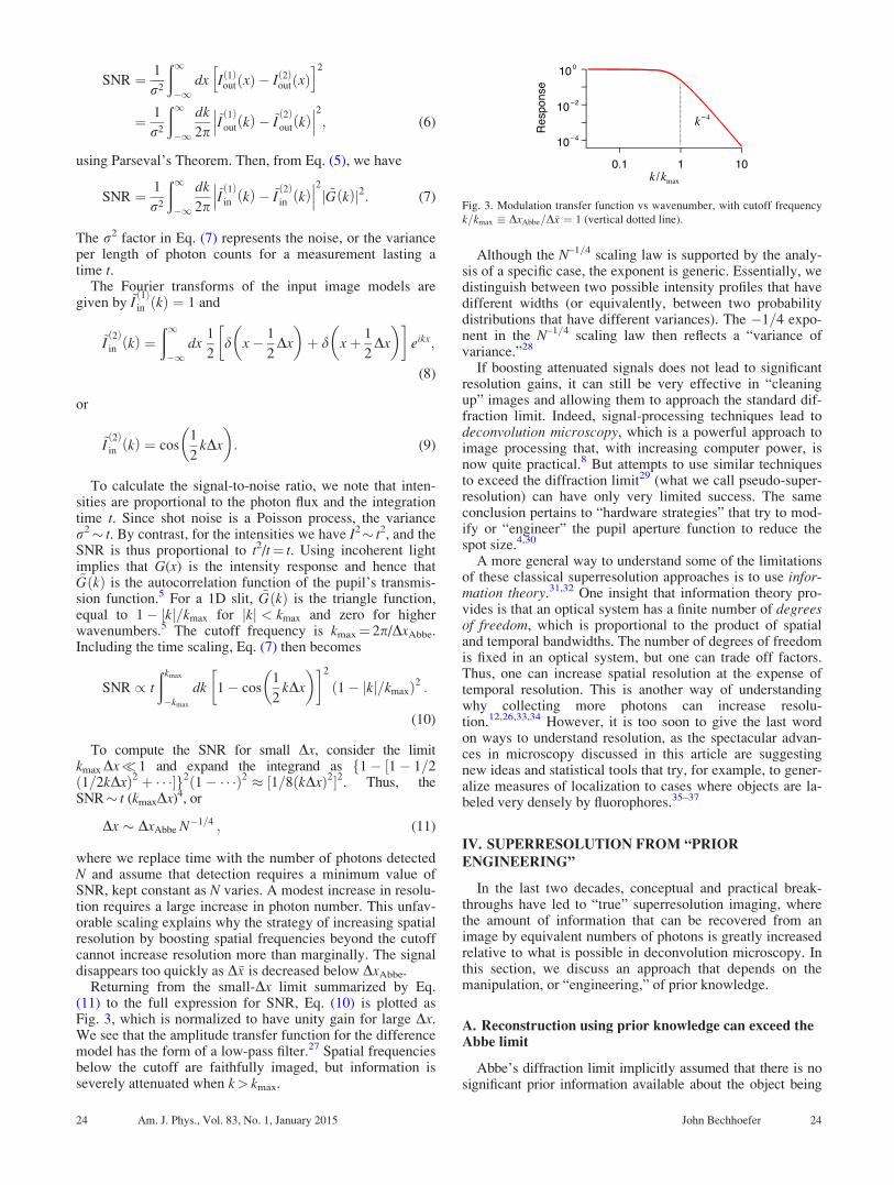
Returning from the small-Dx limit summarized by Eq.(11) to the full expression for SNR, Eq. (10) is plotted asFig. 3, which is normalized to have unity gain for large Dx.We see that the amplitude transfer function for the differencemodel has the form of a low-pass filter.27 Spatial frequenciesbelow the cutoff are faithfully imaged, but information isseverely attenuated when k> kmax.

Although the N–1=4 scaling law is supported by the analy-sis of a specific case, the exponent is generic. Essentially, wedistinguish between two possible intensity profiles that havedifferent widths (or equivalently, between two probabilitydistributions that have different variances). The �1=4 expo-nent in the N–1=4 scaling law then reflects a “variance ofvariance.”28

If boosting attenuated signals does not lead to significantresolution gains, it can still be very effective in “cleaningup” images and allowing them to approach the standard dif-fraction limit. Indeed, signal-processing techniques lead todeconvolution microscopy, which is a powerful approach toimage processing that, with increasing computer power, isnow quite practical.8 But attempts to use similar techniquesto exceed the diffraction limit29 (what we call pseudo-super-resolution) can have only very limited success. The sameconclusion pertains to “hardware strategies” that try to mod-ify or “engineer” the pupil aperture function to reduce thespot size.4,30

A more general way to understand some of the limitationsof these classical superresolution approaches is to use infor-mation theory.31,32 One insight that information theory pro-vides is that an optical system has a finite number of degreesof freedom, which is proportional to the product of spatialand temporal bandwidths. The number of degrees of freedomis fixed in an optical system, but one can trade off factors.Thus, one can increase spatial resolution at the expense oftemporal resolution. This is another way of understandingwhy collecting more photons can increase resolu-tion.12,26,33,34 However, it is too soon to give the last wordon ways to understand resolution, as the spectacular advan-ces in microscopy discussed in this article are suggestingnew ideas and statistical tools that try, for example, to gener-alize measures of localization to cases where objects are la-beled very densely by fluorophores.35–37

IV. SUPERRESOLUTION FROM “PRIOR

ENGINEERING”

In the last two decades, conceptual and practical break-throughs have led to “true” superresolution imaging, wherethe amount of information that can be recovered from animage by equivalent numbers of photons is greatly increasedrelative to what is possible in deconvolution microscopy. Inthis section, we discuss an approach that depends on themanipulation, or “engineering,” of prior knowledge.

A. Reconstruction using prior knowledge can exceed theAbbe limit

Abbe’s diffraction limit implicitly assumed that there is nosignificant prior information available about the object being

Fig. 3. Modulation transfer function vs wavenumber, with cutoff frequency

k=kmax � DxAbbe=D�x ¼ 1 (vertical dotted line).

24 Am. J. Phys., Vol. 83, No. 1, January 2015 John Bechhoefer 24

imaged. When there is, the increase in precision of measure-ments can be spectacular. As a basic example, we consider thelocalization of a single source that we know to be isolated.Here, “localization” contrasts with “resolution,” which per-tains to non-isolated sources. This prior knowledge that thesource is isolated makes all the difference. If we think of ourmeasurement “photon by photon,” the point-spread functionbecomes a unimodal probability distribution whose standarddeviation r0 is set by the Abbe diffraction limit. If we recordN independent photons, then the average has a standard devia-tion �r0=

ffiffiffiffiNp

, as dictated by the Central Limit Theorem.38

Thus, localization improves with increasing photoncounts.39–42 For well-chosen synthetic fluorophores, one candetect Oð104Þ photons, implying localization on the order of ananometer.43 (In live-cell imaging using fluorescent proteins,performance is somewhat worse, as only 100–2000 photonsper fluorophore are typically detectable.44) Again, localizationis not the same as resolution, as it depends on prior informa-tion about the source.

B. Reconstruction without prior knowledge fails

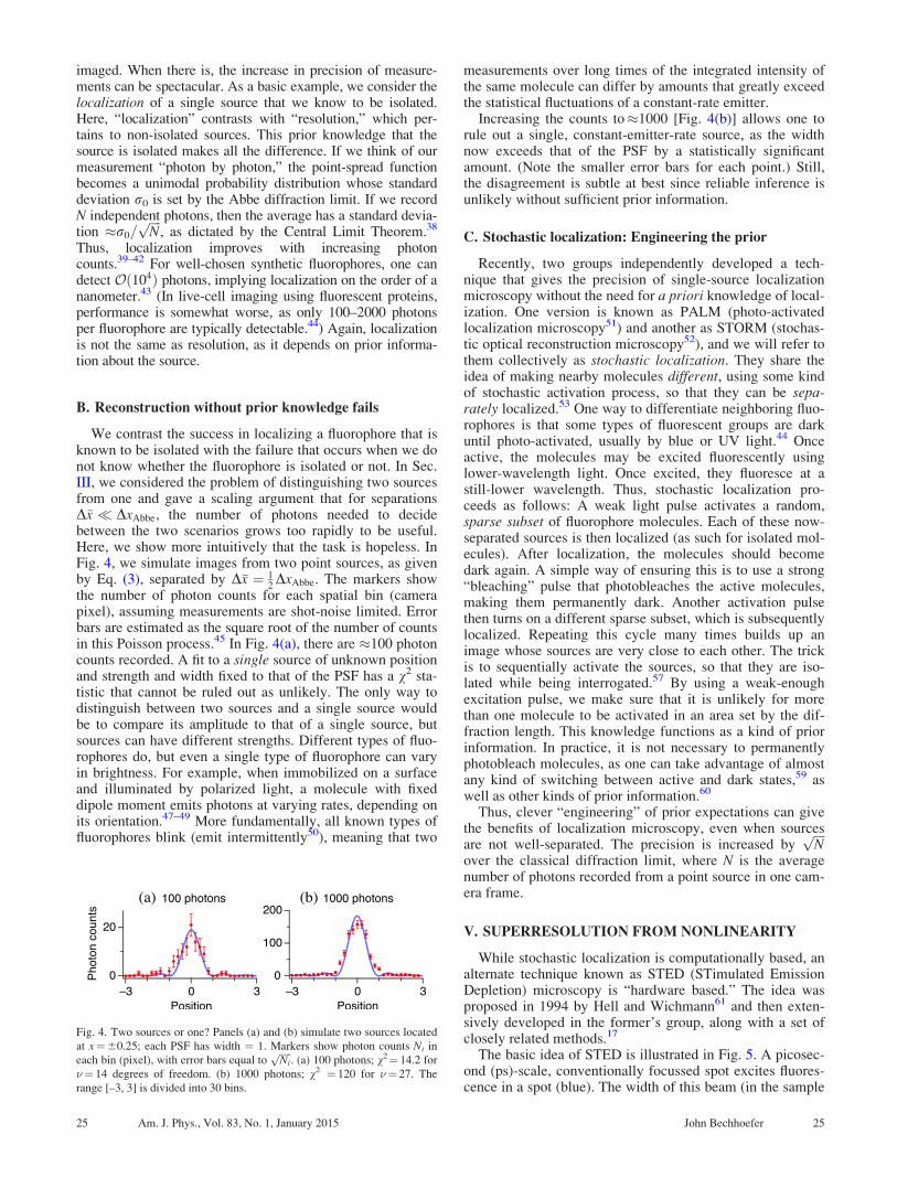
We contrast the success in localizing a fluorophore that isknown to be isolated with the failure that occurs when we donot know whether the fluorophore is isolated or not. In Sec.III, we considered the problem of distinguishing two sourcesfrom one and gave a scaling argument that for separationsD�x � DxAbbe, the number of photons needed to decidebetween the two scenarios grows too rapidly to be useful.Here, we show more intuitively that the task is hopeless. InFig. 4, we simulate images from two point sources, as givenby Eq. (3), separated by D�x ¼ 1

2DxAbbe. The markers show

the number of photon counts for each spatial bin (camerapixel), assuming measurements are shot-noise limited. Errorbars are estimated as the square root of the number of countsin this Poisson process.45 In Fig. 4(a), there are �100 photoncounts recorded. A fit to a single source of unknown positionand strength and width fixed to that of the PSF has a v2 sta-tistic that cannot be ruled out as unlikely. The only way todistinguish between two sources and a single source wouldbe to compare its amplitude to that of a single source, butsources can have different strengths. Different types of fluo-rophores do, but even a single type of fluorophore can varyin brightness. For example, when immobilized on a surfaceand illuminated by polarized light, a molecule with fixeddipole moment emits photons at varying rates, depending onits orientation.47–49 More fundamentally, all known types offluorophores blink (emit intermittently50), meaning that two

measurements over long times of the integrated intensity ofthe same molecule can differ by amounts that greatly exceedthe statistical fluctuations of a constant-rate emitter.

Increasing the counts to�1000 [Fig. 4(b)] allows one torule out a single, constant-emitter-rate source, as the widthnow exceeds that of the PSF by a statistically significantamount. (Note the smaller error bars for each point.) Still,the disagreement is subtle at best since reliable inference isunlikely without sufficient prior information.

C. Stochastic localization: Engineering the prior

Recently, two groups independently developed a tech-nique that gives the precision of single-source localizationmicroscopy without the need for a priori knowledge of local-ization. One version is known as PALM (photo-activatedlocalization microscopy51) and another as STORM (stochas-tic optical reconstruction microscopy52), and we will refer tothem collectively as stochastic localization. They share theidea of making nearby molecules different, using some kindof stochastic activation process, so that they can be sepa-rately localized.53 One way to differentiate neighboring fluo-rophores is that some types of fluorescent groups are darkuntil photo-activated, usually by blue or UV light.44 Onceactive, the molecules may be excited fluorescently usinglower-wavelength light. Once excited, they fluoresce at astill-lower wavelength. Thus, stochastic localization pro-ceeds as follows: A weak light pulse activates a random,sparse subset of fluorophore molecules. Each of these now-separated sources is then localized (as such for isolated mol-ecules). After localization, the molecules should becomedark again. A simple way of ensuring this is to use a strong“bleaching” pulse that photobleaches the active molecules,making them permanently dark. Another activation pulsethen turns on a different sparse subset, which is subsequentlylocalized. Repeating this cycle many times builds up animage whose sources are very close to each other. The trickis to sequentially activate the sources, so that they are iso-lated while being interrogated.57 By using a weak-enoughexcitation pulse, we make sure that it is unlikely for morethan one molecule to be activated in an area set by the dif-fraction length. This knowledge functions as a kind of priorinformation. In practice, it is not necessary to permanentlyphotobleach molecules, as one can take advantage of almostany kind of switching between active and dark states,59 aswell as other kinds of prior information.60

Thus, clever “engineering” of prior expectations can givethe benefits of localization microscopy, even when sourcesare not well-separated. The precision is increased by

ffiffiffiffiNp

over the classical diffraction limit, where N is the averagenumber of photons recorded from a point source in one cam-era frame.

V. SUPERRESOLUTION FROM NONLINEARITY

While stochastic localization is computationally based, analternate technique known as STED (STimulated EmissionDepletion) microscopy is “hardware based.” The idea wasproposed in 1994 by Hell and Wichmann61 and then exten-sively developed in the former’s group, along with a set ofclosely related methods.17

The basic idea of STED is illustrated in Fig. 5. A picosec-ond (ps)-scale, conventionally focussed spot excites fluores-cence in a spot (blue). The width of this beam (in the sample

Fig. 4. Two sources or one? Panels (a) and (b) simulate two sources located

at x¼60.25; each PSF has width ¼ 1. Markers show photon counts Ni in

each bin (pixel), with error bars equal toffiffiffiffiffiNi

p. (a) 100 photons; v2¼ 14.2 for

�¼ 14 degrees of freedom. (b) 1000 photons; v2 ¼ 120 for �¼ 27. The

range [–3, 3] is divided into 30 bins.

25 Am. J. Phys., Vol. 83, No. 1, January 2015 John Bechhoefer 25

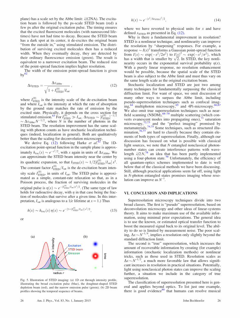
plane) has a scale set by the Abbe limit: k/(2NA). The excita-tion beam is followed by the ps-scale STED beam (red) afew ps after the original excitation pulse. The timing ensuresthat the excited fluorescent molecules (with nanosecond life-times) have not had time to decay. Because the STED beamhas a dark spot at its center, it de-excites the original beam“from the outside in,” using stimulated emission. The distri-bution of surviving excited molecules then has a reducedwidth. When they eventually decay, they are detected bytheir ordinary fluorescence emission (green). The result isequivalent to a narrower excitation beam. The reduced sizeof the point-spread function implies higher resolution.

The width of the emission point-spread function is givenby62

DxSTED ¼DxAbbeffiffiffiffiffiffiffiffiffiffiffiffiffiffiffiffiffiffiffiffiffiffiffiffiffiffiffi

1þ I 0ð ÞSTED=Isat

q ; (12)

where Ið0ÞSTED is the intensity scale of the de-excitation beam

and where Isat is the intensity at which the rate of absorptionby the ground state matches the rate of emission by theexcited state. Physically, it depends on the cross section forstimulated emission.63 For I

ð0ÞSTED � Isat; DxSTED � ½Ið0ÞSTED

�1=2

� DxAbbe N�1=2, where N is the number of photons in theSTED beam. The resolution improvement has the same scal-ing with photon counts as have stochastic localization techni-ques (indeed, localization in general). Both are qualitativelybetter than the scaling for deconvolution microscopy.

We derive Eq. (12) following Harke et al.62 The 1D-excitation point-spread function in the sample plane is approx-

imately hexcðxÞ � e�x2=2, with x again in units of DxAbbe. Wecan approximate the STED beam intensity near the center by

its quadratic expansion, so that ISTEDðxÞ � 1=2½Ið0ÞSTED=Isat x2.

The constant factor Ið0ÞSTED=Isat is the de-excitation beam inten-

sity scale Ið0ÞSTED, in units of Isat. The STED pulse is approxi-

mated as a simple, constant-rate relaxation so that, as in aPoisson process, the fraction of surviving molecules in the

original pulse is gðxÞ � e�ðIð0ÞSTED

=IsatÞx2=2. (The same type of lawholds for radioactive decay, with g in that case being the frac-tion of molecules that survive after a given time. In this inter-pretation, Isat is analogous to a 1/e lifetime at x¼ 1.) Thus

hðxÞ � hexcðxÞ gðxÞ � e�½1þðIð0ÞSTED

=IsatÞ x2=2; (13)

or

hðxÞ � e�ðx2=DxSTEDÞ2=2; (14)

where we have reverted to physical units for x and havedefined xSTED as presented in Eq. (12).

Why is there a fundamental improvement in resolution?STED is a nonlinear technique, and nonlinearity can improvethe resolution by “sharpening” responses. For example, aresponse � I(x)2 transforms a Gaussian point-spread functionfrom IðxÞ � expð�x2=2r2Þ to IðxÞ2 � expð�x2=r2Þ, whichhas a width that is smaller by

ffiffiffi2p

. In STED, the key nonli-nearity occurs in the exponential survival probability g(x).With a purely linear response, no resolution enhancementwould be possible, because the spatial scale of the STEDbeam is also subject to the Abbe limit and must thus vary onthe same length scale as the original excitation beam.

Stochastic localization and STED are just two amongmany techniques for fundamentally surpassing the classicaldiffraction limit. For want of space, we omit discussion ofmany other ways to surpass the Abbe limit, includingpseudo-superresolution techniques such as confocal imag-ing,64 multiphoton microscopy,65 and 4Pi-microscopy.66,67

We also omit true superresolution techniques such as near-field scanning (NSOM),68–70 multiple scattering (which con-verts evanescent modes into propagating ones),71 saturationmicroscopy,72,73 and the “perfect imaging” promised bymetamaterials.74,75 Some techniques, such as structured illu-mination,76,77 are hard to classify because they contain ele-ments of both types of superresolution. Finally, although ourdiscussion has focused on what is possible with classicallight sources, we note that N entangled nonclassical photon-number states can create interference patterns with wave-length k/2 N,78 an idea that has been partly implementedusing a four-photon state.79 Unfortunately, the efficiency ofall quantum-optics schemes implemented to date is wellbelow that of the classical methods we have been discussing.Still, although practical applications seem far off, using lightin N-photon entangled states promises imaging whose reso-lution can improve as N–1.

VI. CONCLUSION AND IMPLICATIONS

Superresolution microscopy techniques divide into twobroad classes. The first is “pseudo” superresolution, based ondeconvolution microscopy and other ideas of linear-systemstheory. It aims to make maximum use of the available infor-mation, using minimal prior expectations. The general ideais to use the known, or estimated optical transfer function toboost the measured signal back to its original level. The abil-ity to do so is limited by measurement noise. The poor scal-ing, Dx�N–1=4, implies a resolution only slightly beyond thestandard diffraction limit.

The second is “true” superresolution, which increases theamount of recoverable information by creating (for example)information (stochastic localization methods) or nonlineartricks, such as those used in STED. Resolution scales asDx�N–1=2, a much more favorable law that allows signifi-cant increases in resolution in practical situations. Potentially,light using nonclassical photon states can improve the scalingfurther, a situation we include in the category of truesuperresolution.

The classification of superresolution presented here is gen-eral and applies beyond optics. To list just one example,there is good evidence80 that humans can resolve musical

Fig. 5. Illustration of STED imaging: (a) 1D cut through intensity profile,

illustrating the broad excitation pulse (blue), the doughnut-shaped STED

depletion beam (red), and the narrow emission pulse (green); (b) 2D beam

profiles showing the temporal sequence of beams.

26 Am. J. Phys., Vol. 83, No. 1, January 2015 John Bechhoefer 26

pitch much better than the classic time-frequency uncertaintyprinciple, which states that the product DtDf 1/(4p), whereDt is the time a note is played and Df the difference in pitchto be distinguished. Since humans can routinely beat thislimit, Oppenheim and Magnasco conclude that the ear and/orbrain must use nonlinear processing.80 But louder soundswill also improve pitch resolution, in analogy with our dis-cussion of light intensity and low-pass filtering, an effectthey do not discuss. Whether “audio superresolution” is dueto high signal levels or to nonlinear processing, the ideas pre-sented are perhaps useful for understanding the limits topitch resolution.

The questions about superresolution that we have exploredhere in the context of microscopy (and, briefly, human hear-ing) apply in some sense to any measurement problem.Thus, understanding what limits measurements, and appreci-ating the roles of signal-to-noise ratio and of prior expecta-tions, should be part of the education of a physicist.

ACKNOWLEDGMENTS

The author thanks Jari Lindberg and Jeff Salvail for acareful reading of the manuscript and for valuablesuggestions. This work was supported by NSERC (Canada).

APPENDIX: DECISION MAKING AND THE SIGNAL-

TO-NOISE RATIO

To justify more carefully the link between likelihood andsignal-to-noise ratios, we follow Harris14 and consider theproblem of deciding whether a given image comes fromobject 1 or object 2 (see Fig. 2). If the measured intensitywere noiseless, the one-dimensional image would be eitherIð1ÞoutðxÞ or I

ð2ÞoutðxÞ. Let the image have pixels indexed by i that

are centered on xi, of width Dx. Let the measured intensity ateach pixel be Ii. The noise variance in one pixel r2

p is due toshot noise, read noise, and dark noise, and its distribution isassumed Gaussian and independent of i, for simplicity. (Ifthe intensity varies considerably over the image, then we candefine a rp that represents an average noise level.) The likeli-hood that the image comes from object 1 is then

L 1ð Þ �Y

i

1ffiffiffiffiffiffi2pp

rp

e� Ii�I 1ð Þi½ 2=2r2

p ; (A1)

where Ið1Þi � I

ð1ÞoutðxÞjx¼xi

Dx is the number of photons detectedin pixel i and the product is over all pixels in the detector.An analogous expression holds for L(2). Then the natural log-arithm of the likelihood ratio is given by

w12 � lnL 1ð Þ

L 2ð Þ ¼1

2r2p

Xi

Ii � I 2ð Þi

h i2

� Ii � I 1ð Þi

h i2�

:

(A2)

If object 1 actually produces the image, then Ii ¼ Ið1Þi þ ni,

and Eq. (A2) becomes

w12 ¼X

i

1

2r2p

I 1ð Þi � I 2ð Þ

i

h i2

� 2ni

2r2p

I 1ð Þi � I 2ð Þ

i

h i( ):

(A3)

If ni is Gaussian, then so is w12; its mean is given by

hwi ¼ 1=ð2r2pÞP

i½Ið1Þi � I

ð2Þi

2and its variance by r2

w

¼ 1=ðr2pÞP

i½Ið1Þi � I

ð2Þi

2. We will conclude that object 1

produced the image if the random variable w12> 0. Theprobability that our decision is correct is thus given by

P w12 > 0ð Þ ¼ 1ffiffiffiffiffiffi2pp

rw

ð10

dw e� w�hwið Þ2=2r2w

¼ 1ffiffiffiffiffiffi2pp

ð1�hwi=rw

dz e�z2=2; (A4)

or

P w12 > 0ð Þ ¼ 1

21þ erf

ffiffiffiffiffiffiffiffiffiffiSNRp ��

; (A5)

where the error function erfðxÞ ¼ ð2=ffiffiffippÞÐ x

0du e�u2

. Thisresult depends only on 2hwi=rw �

ffiffiffiffiffiffiffiffiffiffiSNRp

. Below, we showSNR to be the signal-to-noise ratio. For SNR� 1, the proba-bility of a wrong decision is

1� P w12 > 0ð Þ � 1ffiffiffiffiffiffiffiffiffiffiffiffiffiffiffiffi4p SNRp e�SNR ; (A6)

which rapidly goes to zero for large SNR. To further inter-pret the SNR, we write

SNR ¼ 2hwirw

!2

¼4r2

p

4r4p

Xi

I 1ð Þi � I 2ð Þ

i

h i2�

; (A7)

or

SNR � Dx

r2p

ð1�1

dx I 1ð Þout xð Þ � I 2ð Þ

out xð Þh i2�

: (A8)

Defining r2 ¼ r2p=Dx to be the photon variance per length

gives Eq. (6). Recalling that Iout (x) is the number of photonsdetected per length in the absence of noise, we verify thatthe right-hand side of Eq. (A8) is dimensionless. Thus,ffiffiffiffiffiffiffiffiffiffi

SNRp

is the ratio of the photon count difference to the pho-ton count fluctuation over a given length of the image.

a)Electronic mail: johnb@sfu.ca1H. Volkmann, “Ernst Abbe and his work,” Appl. Opt. 5, 1720–1731

(1966).2L. Rayleigh, “On the theory of optical images, with special reference to

the microscope,” The London, Edinburgh, Dublin Philos. Mag. J. Sci.

42(XV), 167–195 (1896).3A. B. Porter, “On the diffraction theory of microscopic vision,” The

London, Edinburgh, Dublin Philos. Mag. J. Sci. 11, 154–166 (1906).4G. Toraldo di Francia, “Super-gain antennas and optical resolving power,”

Nuovo Cimento Suppl. 9, 426–438 (1952).5J. W. Goodman, Introduction to Fourier Optics, 3rd ed. (Roberts and

Company Publishers, Greenwood Village, CO, 2005). The first edition

was published in 1968.6F. M. Huang and N. I. Zheludev, “Super-resolution without evanescent

waves,” Nano Lett. 9, 1249–1254 (2009). The authors give a modern imple-

mentation of the aperture schemes pioneered by Toraldo Di Francia (Ref. 4).7“Superresolution” is also sometimes used to describe sub-pixel resolution

in an imaging detector. Since pixels are not necessarily related to intrinsic

resolution, we do not consider such techniques here.8J.-B. Sibarita, “Deconvolution microscopy,” Adv. Biochem. Engin.

Biotechnol. 95, 201–243 (2005).

27 Am. J. Phys., Vol. 83, No. 1, January 2015 John Bechhoefer 27

9Superresolution fluorescence microscopy was the 2008 “Method of the

Year” for Nature Methods, and its January 2009 issue contains commen-

tary and interviews with scientists playing a principal role in its develop-

ment. This is a good “cultural” reference.10B. O. Leung and K. C. Chou, “Review of superresolution fluorescence mi-

croscopy for biology,” Appl. Spectrosc. 65, 967–980 (2011).11For example, a STED microscope is sold by the Leica Corporation.12C. J. R. Sheppard, “Fundamentals of superresolution,” Micron 38,

165–169 (2007). Sheppard introduces three classes rather than two:

Improved superresolution boosts spatial frequency response but leaves the

cutoff frequency unchanged. Restricted superresolution includes tricks that

increase the cut-off by up to a factor of two. We use “pseudo” superresolu-

tion for both cases. Finally, unrestricted superresolution refers to what we

term “true” superresolution.13J. Mertz, Introduction to Optical Microscopy (Roberts and Co.,

Greenwood Village, CO, 2010), Chap. 18. Mertz follows Sheppard’s clas-

sification, giving a simple but broad overview.14J. L. Harris, “Resolving power and decision theory,” J. Opt. Soc. Am. 54,

606–611 (1964).15An updated treatment of the one-point-source-or-two decision problem

is given by A. R. Small, “Theoretical limits on errors and acquisition

rates in localizing switchable fluorophores,” Biophys. J. 96, L16–L18

(2009).16For a more formal Bayesian treatment, see S. Prasad, “Asymptotics of

Bayesian error probability and source super-localization in three

dimensions,” Opt. Express 22, 16008–16028 (2014).17S. W. Hell, “Far-field optical nanoscopy,” Springer Ser. Chem. Phys. 96,

365–398 (2010).18B. Huang, H. Babcock, and X. Zhuang, “Breaking the diffraction barrier:

Superresolution imaging of cells,” Cell 143, 1047–1058 (2010).19C. Cremer and B. R. Masters, “Resolution enhancement techniques in

microscopy,” Eur. Phys. J. H 38, 281–344 (2013).20E. Hecht, Optics, 4th ed. (Addison-Wesley, Menlo Park, CA, 2002), Chap.

13.21G. Brooker, Modern Classical Optics (Oxford U.P., New York, 2002),

Chap. 12.22A. Lipson, S. G. Lipson, and H. Lipson, Optical Physics, 4th ed.

(Cambridge U.P., Cambridge, UK, 2011), Chap. 12. This edition of a well-

established text adds a section on superresolution techniques, with a view

that complements the one presented here.23Equation (1) gives the lateral resolution. The resolution along the optical

axis is poorer: d ¼ k=ðn sin2aÞ.24However, the magnification of an objective does not determine its

resolution.25P. M. Duffieux, The Fourier Transform and Its Applications to Optics, 2nd

ed. (John Wiley & Sons, Hoboken, NJ, 1983). The first edition, in French,

was published in 1946. Duffieux formulated the idea of the optical transfer

function in the 1930s.26J. Lindberg, “Mathematical concepts of optical superresolution,” J. Opt.

14, 083001 (2012).27A subtle point: The modulation transfer function is zero beyond a finite

spatial frequency; yet the response in Fig. 3 is non-zero at all frequencies.

The explanation is that an object of finite extent has a Fraunhofer diffrac-

tion pattern (Fourier transform) that is analytic, neglecting noise. Analytic

functions are determined by any finite interval (analytic continuation),

meaning that one can, in principle, extrapolate the bandwidth and deduce

the exact behavior beyond the cutoff from that inside the cutoff. In prac-

tice, noise cuts off the information (Fig. 3). See Lucy (Ref. 28) for a brief

discussion and Goodman’s book (Ref. 5) for more detail.28L. B. Lucy, “Statistical limits to superresolution,” Astron. Astrophys. 261,

706–710 (1992). Lucy does not assume the PSF width to be known and

thus reaches the more pessimistic conclusion that Dx�N�1=8 . Since the

second moments are then matched, one has to use the variance of the

fourth moment to distinguish the images.29K. Pich�e, J. Leach, A. S. Johnson, J. Z. Salvail, M. I. Kolobov, and R. W.

Boyd, “Experimental realization of optical eigenmode superresolution,”

Opt. Express 20, 26424 (2012). Instruments with finite aperture sizes have

discrete eigenmodes (that are not simple sines and cosines), which should

be used for more accurate image restoration.30E. Ramsay, K. A. Serrels, A. J. Waddie, M. R. Taghizadeh, and D. T.

Reid, “Optical superresolution with aperture-function engineering,” Am. J.

Phys. 76, 1002–1006 (2008).31G. Toraldo di Francia, “Resolving power and information,” J. Opt. Soc.

Am. 45, 497–501 (1955).

32S. G. Lipson, “Why is superresolution so inefficient?” Micron 34,

309–312 (2003).33W. Lukosz, “Optical systems with resolving powers exceeding the classi-

cal limit,” J. Opt. Soc. Am. 56, 1463–1472 (1966).34W. Lukosz, “Optical systems with resolving powers exceeding the classi-

cal limit. II,” J. Opt. Soc. Am. 57, 932–941 (1967).35E. A. Mukamel and M. J. Schnitzer, “Unified resolution bounds for con-

ventional and stochastic localization fluorescence microscopy,” Phys. Rev.

Lett. 109, 168102-1–5 (2012).36J. E. Fitzgerald, J. Lu, and M. J. Schnitzer, “Estimation theoretic measure

of resolution for stochastic localization microscopy,” Phys. Rev. Lett. 109,

048102-1–5 (2012).37R. P. J. Nieuwenhuizen, K. A. Lidke, M. Bates, D. L. Puig, D. Gr€onwald,

S. Stallinga, and B. Rieger, “Measuring image resolution in optical nano-

scopy,” Nat. Methods 10, 557–562 (2013).38D. S. Sivia and J. Skilling, Data Analysis: A Bayesian Tutorial, 2nd ed.

(Oxford U.P., New York, 2006), Chap. 5.39N. Bobroff, “Position measurement with a resolution and noise-limited

instrument,” Rev. Sci. Instrum. 57, 1152–1157 (1986).40R. J. Ober, S. Ram, and E. S. Ward, “Localization accuracy in single-

molecule microscopy,” Biophys. J. 86, 1185–1200 (2004).41K. I. Mortensen, L. S. Churchman, J. A. Spudich, and H. Flyvbjerg,

“Optimized localization analysis for single-molecule tracking and superre-

solution microscopy,” Nat. Methods 7, 377–381 (2010). Gives a useful

assessment of various position estimators.42H. Deschout, F. C. Zanacchi, M. Mlodzianoski, A. Diaspro, J.

Bewersdorf, S. T. Hess, and K. Braeckmans, “Precisely and accurately

localizing single emitters in fluorescence microscopy,” Nat. Methods 11,

253–266 (2014).43A. Yildiz and P. R. Selvin, “Fluorescence imaging with one nanometer ac-

curacy: Application to molecular motors,” Acc. Chem. Res. 38, 574–582

(2005).44G. Patterson, M. Davidson, S. Manley, and J. Lippincott-Schwartz,

“Superresolution imaging using single-molecule localization,” Annu. Rev.

Phys. Chem. 61, 345–367 (2010).45One should set the errors to be the square root of the smooth distribu-

tion value deduced from the initial fit and then iterate the fitting pro-

cess (Ref. 46). The conclusions however, would not change, in this

case.46S. F. Nørrelykke and H. Flyvbjerg, “Power spectrum analysis with least-

squares fitting: Amplitude bias and its elimination, with application to op-

tical tweezers and atomic force microscope cantilevers,” Rev. Sci. Inst. 81,

075103-1–16 (2010).47E. Betzig and R. J. Chichester, “Single molecules observed by near-field

scanning optical microscopy,” Science 262, 1422–1425 (1993).48T. Ha, T. A. Laurence, D. S. Chemla, and S. Weiss, “Polarization spectros-

copy of single fluorescent molecules,” J. Phys. Chem. B 103, 6839–6850

(1999).49J. Engelhardt, J. Keller, P. Hoyer, M. Reuss, T. Staudt, and S. W. Hell,

“Molecular orientation affects localization accuracy in superresolution far-

field fluorescence microscopy,” Nano. Lett. 11, 209–213 (2011).50P. Frantsuzov, M. Kuno, B. Jank�o, and R. A. Marcus, “Universal emission

intermittency in quantum dots, nanorods and nanowires,” Nat. Phys. 4,

519–522 (2008).51E. Betzig, G. H. Patterson, R. Sougrat, O. W. Lindwasser, S. Olenych, J.

S. Bonifacino, M. W. Davidson, J. Lippincott-Schwartz, and H. F. Hess,

“Imaging intracellular fluorescent proteins at nanometer resolution,”

Science 313, 1642–1645 (2006).52M. J. Rust, M. Bates, and X. Zhuang, “Sub-diffraction-limit imaging by

stochastic optical reconstruction microscopy (STORM),” Nat. Methods 3,

793–795 (2006).53Important precursors in using sequential localization to develop stochastic

localization techniques such as PALM and STORM were Qu et al. (Ref.

54) and Lidke et al. (Ref. 55) Stochastic localization was also independ-

ently developed by Hess et al. (Ref. 56).54X. Qu, D. Wu, L. Mets, and N. F. Scherer, “Nanometer-localized multiple

single-molecule fluorescence microscopy,” Proc. Natl. Acad. Sci. U.S.A

101, 11298–11303 (2004).55K. A. Lidke, B. Rieger, T. M. Jovin, and R. Heintzmann, “Superresolution

by localization of quantum dots using blinking statistics,” Opt. Express 13,

7052–7062 (2005).56S. T. Hess, T. P. K. Girirajan, and M. D. Mason, “Ultra-high resolution

imaging by fluorescence photoactivation localization microscopy,”

Biophys. J. 91, 4258–4272 (2006).

28 Am. J. Phys., Vol. 83, No. 1, January 2015 John Bechhoefer 28

57Sparseness can improve resolution in other ways, as well. For example,

the new field of compressive sensing also uses a priori knowledge that a

sparse representation exists in a clever way to improve resolution

(Ref. 58).58H. P. Babcock, J. R. Moffitt, Y. Cao, and X. Zhuang, “Fast compressed

sensing analysis for super-resolution imaging using L1-homotopy,” Opt.

Express 21, 28583–28596 (2013).59T. Dertinger, R. Colyer, G. Iyer, S. Weiss, and J. Enderlein, “Fast,

background-free, 3D super-resolution optical fluctuation imaging (SOFI),”

Proc. Natl. Acad. Sci. U.S.A 106, 22287–22292 (2009). This clever tech-

nique uses intensity fluctuations due to multiple switching between two

states of different brightness.60A. J. Berro, A. J. Berglund, P. T. Carmichael, J. S. Kim, and J. A. Liddle,

“Super-resolution optical measurement of nanoscale photoacid distribution

in lithographic materials,” ACS Nano 6, 9496–9502 (2012). If one knows

that vertical stripes are present, one can sum localizations by column to

get a higher-resolution horizontal cross-section.61S. W. Hell and J. Wichmann, “Breaking the diffraction resolution limit by

stimulated emission: Stimulated-emission-depletion fluorescence micro-

scopy,” Opt. Lett. 19, 780–782 (1994).62B. Harke, J. Keller, C. K. Ullal, V. Westphal, A. Sch€onle, and S. W. Hell,

“Resolution scaling in STED microscopy,” Opt. Express 16, 4154–4162 (2008).63M. Dyba, J. Keller, and S. W. Hell, “Phase filter enhanced STED-4Pi fluores-

cence microscopy: Theory and experiment,” New J. Phys. 7, Article 134

(2005), pp. 21.64J. B. Pawley, Handbook of Biological Confocal Microscopy, 2nd ed.

(Springer, New York, 2006).65A. Diaspro, G. Chirico, and M. Collini, “Two-photon fluorescence excita-

tion and related techniques in biological microscopy,” Quart. Rev.

Biophys. 38, 97–166 (2005).66C. Cremer and T. Cremer, “Considerations on a laser-scanning-microscope

with high resolution and depth of field,” Microsc. Acta 81, 31–44 (1978).67S. Hell and E. H. K. Stelzer, “Fundamental improvement of resolution

with a 4Pi-confocal fluorescence microscope using two-photon

excitation,” Opt. Commun. 93, 277–282 (1992).

68E. H. Synge, “A suggested method for extending microscopic resolution

into the ultra-microscopic region,” Philos. Mag. 6, 356–362 (1928).69E. Betzig, A. Lewis, A. Harootunian, M. Isaacson, and E. Kratschmer,

“Near-field scanning optical microscopy (NSOM): Development and bio-

physical applications,” Biophys. J. 49, 269–279 (1986).70L. Novotny and B. Hecht, Principles of Nano-Optics, 2nd ed. (Cambridge

U.P., Cambridge, UK, 2012).71F. Simonetti, “Multiple scattering: The key to unravel the subwavelength

world from the far-field pattern of a scattered wave,” Phys. Rev. E 73,

036619-1–13 (2006).72R. Heintzmann, T. M. Jovin, and C. Cremer, “Saturated patterned excita-

tion microscopy—a concept for optical resolution improvement,” J. Opt.

Soc. Am. A 19, 1599–1609 (2002).73K. Fujita, M. Kobayashi, S. Kawano, M. Yamanaka, and S. Kawata,

“High-resolution confocal microscopy by saturated excitation of fluo-

rescence,” Phys. Rev. Lett. 99, 228105-1–4 (2007).74J. B. Pendry, “Negative refraction makes a perfect lens,” Phys. Rev. Lett.

85, 3966–3969 (2000).75N. Fang, H. Lee, C. Sun, and X. Zhang, “Sub-diffraction-limited optical

imaging with a silver superlens,” Science 308, 534–537 (2005).76M. G. L. Gustafsson, “Surpassing the lateral resolution limit by a factor of

two using structured illumination microscopy,” J. Microsc. 198, 82–87

(2000).77M. G. L. Gustafsson, “Nonlinear structured-illumination microscopy:

Wide-field fluorescence imaging with theoretically unlimited resolution,”

Proc. Natl. Acad. Sci. U.S.A 102, 13081–13086 (2005).78A. N. Boto, P. Kok, D. S. Abrams, S. L. Braunstein, C. P. Williams, and J.

P. Dowling, “Quantum interferometric optical lithography: Exploiting

entanglement to beat the diffraction limit,” Phys. Rev. Lett. 85,

2733–2736 (2000).79L. A. Rozema, J. D. Bateman, D. H. Mahler, R. Okamoto, A. Feizpour, A.

Hayat, and A. M. Steinberg, “Scalable spatial superresolution using

entangled photons,” Phys. Rev. Lett. 112, 223602-1–5 (2014).80J. N. Oppenheim and M. O. Magnasco, “Human time-frequency acuity beats

the Fourier Uncertainty principle,” Phys. Rev. Lett. 110, 044301-1–5 (2013).

29 Am. J. Phys., Vol. 83, No. 1, January 2015 John Bechhoefer 29