What Is Wrong with "What Is Wrong with MEM?"

What Is Wrong with "What Is Wrong with MEM?"

G E R V A I S L E C L E R C and J . J . P I R E A U X * Laboratoire Interdisciplinaire de Spectroscopie Electronique, Facultds Universitaires Notre-Dame de la Paix, Rue de Bruxelles 61, B-5000 Namur, Belgium

A theoretical derivation of autoregressive spectral estimation is briefly presented, at variance with a recent paper by Kauppinen and Saario. Index Headings: Signal analysis; AR spectral estimation.

I N T R O D U C T I O N

Kauppinen and Saario have recently published a paper ~ in which they take a strong stance against the use of the Maximum Entropy Method (MEM) for spectral estimation. They claim to have shown theoretically and by the use of examples that the MEM power spectral estimator is a very bad approximation of the true power spectrum of a random signal. They also state that the only way to properly carry out resolution enhancement is to use the Fourier transform of the signal.

We hereby wish to express our disagreement with these views. After briefly presenting the signal theory under- lying the autoregressive method of spectral estimation, we will discuss the arguments of Kauppinen and Saario and present counterpoints to statements with which we disagree.

T H E O R Y

Stationary Signals and Linear Filters. A convenient way of expressing a discrete random signal xn(Xo, x~, x2 • . . ) is to consider it as the output of a linear filter B(z) whose input is the stationary and uncorrelated (white- noise) sequence en :2'3

e.---~ [B(z)] ---~x. (1)

where B(z) can be expressed as co

B(z) = ~ b .z -" (2) n=O

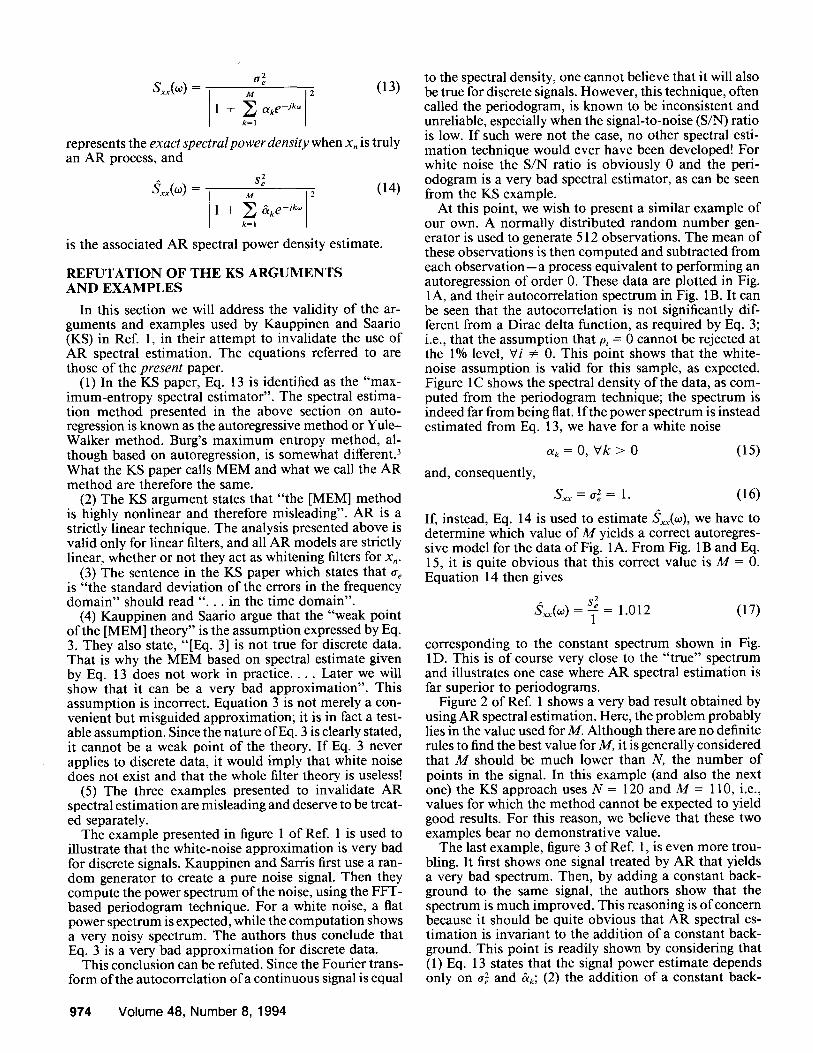
with z-" = e -j~". The condition of white noise implies that

E[efj] = ¢$60 (3)

where ere 2 stands for the variance ofe, (in the time domain), and El. ] represents the expectancy operator. The variance is usually adjusted to have b0 = 1. The output signal is then given by

x . = ~ b._~e, (4) i=O

and 1/B(z) acts as a whitening filter for x.:

X n ~ ~ ~ e n. (5)

Received 18 November 1993; accepted 13 May 1994. * Author to whom correspondence should be sent.

As shown by Wold, 4 this representation can be used to model any stationary signal x, . With the use of the spectral factofization theorem, 5 it can then be shown that the spectral power density of Xn is given by:

Sxx(O~) = Cre 2 I B(o~) I a. (6)

We wish to insist upon the fact that, under the as- sumptions stated above, Eq. 6 is not an approximation but an exact expression. Therefore, the problem of esti- mating the spectral power density of any discrete stationary signal x , can be reduced to the problem of finding a whitening filter for Xn and then applying Eq. 6.

Autoregression. Autoregressive modeling (AR) is one possible way of finding a whitening filter for the time- domain signal x, . Suppose that each observation of the sequence Xn can be expressed by a linear combination of the M preceding observations:

M

Xn -- Z OikXn--k = e.. (7) k=l

It is then said that x . is autoregressive. For the AR model of order M, a set of predicted values

2 y can be estimated according to M

)~M = __ Z OlkXn--k ( 8 ) k=l

x. - 27 M = e. u (9)

where the &k are least-squares estimates of the ak, and e~nn stands for the autoregression residuals. If x. can be efficiently expressed by an AR model of order M, it implies that

2 (lO) Var(e~) = Se 2 ~ ae

and

E[effe) ~~] ~ fie260. (1 1)

This last formula suggests that testing the residuals for the presence of serial correlation constitutes a convenient way of testing the validity of the AR model; 6 if no sig- nificant serial correlation is detected, then x, can be as- sumed to have been properly modeled. When such is the case, it implies that the autoregressive model acts as a whitening filter for xn and that Eq. 6 can be used for spectral estimation.

The transfer function of the autoregressive model is simply given by 2

1 B~R(Z) = M (12)

1 + ~ a k Z - k k=l

and, from Eq. 6 and 10, it immediately follows that

Volume 48, Number 8, 1994 0003.7028/94/4808-097352.00/0 APPLIED SPECTROSCOPY 973 © 1994 Society for Applied Spectroscopy

~e ~ Sxx(w) = 2 (13)

represents the exact spectralpower density when x. is truly an AR process, and

~xx(w) = see (14) 2

1 + ~ &ke -jk~ k=|

is the associated AR spectral power density estimate.

REFUTATION OF THE KS A R G U M E N T S AND EXAMPLES

In this section we will address the validity of the arguments and examples used by Kauppinen and Saario (KS) in Ref. 1, in their attempt to invalidate the use of AR spectral estimation. The equations referred to are those of the present paper.

(1) In the KS paper, Eq. 13 is identified as the "maximum-entropy spectral estimator". The spectral estimation method presented in the above section on autoregression is known as the autoregressive method or Yule- Walker method. Burg's maximum entropy method, although based on autoregression, is somewhat different? What the KS paper calls MEM and what we call the AR method are therefore the same.

(2) The KS argument states that "the [MEM] method is highly nonlinear and therefore misleading". AR is a strictly linear technique. The analysis presented above is valid only for linear filters, and all AR models are strictly linear, whether or not they act as whitening filters for x,.

(3) The sentence in the KS paper which states that ae is "the standard deviation of the errors in the frequency domain" should read " . . . in the time domain".

(4) Kauppinen and Saario argue that the "weak point of the [MEM] theory" is the assumption expressed by Eq. 3. They also state, "[Eq. 3] is not true for discrete data. That is why the MEM based on spectral estimate given by Eq. 13 does not work in practice . . . . Later we will show that it can be a very bad approximation". This assumption is incorrect. Equation 3 is not merely a convenient but misguided approximation; it is in fact a test- able assumption. Since the nature ofEq. 3 is clearly stated, it cannot be a weak point of the theory. If Eq. 3 never applies to discrete data, it would imply that white noise does not exist and that the whole filter theory is useless!

(5) The three examples presented to invalidate AR spectral estimation are misleading and deserve to be treated separately.

The example presented in figure 1 of Ref. 1 is used to illustrate that the white-noise approximation is very bad for discrete signals. Kauppinen and Sarris first use a random generator to create a pure noise signal. Then they compute the power spectrum of the noise, using the FFT- based periodogram technique. For a white noise, a flat power spectrum is expected, while the computation shows a very noisy spectrum. The authors thus conclude that Eq. 3 is a very bad approximation for discrete data.

This conclusion can be refuted. Since the Fourier transform of the autocorrelation of a continuous signal is equal

to the spectral density, one cannot believe that it will also be true for discrete signals. However, this technique, often called the periodogram, is known to be inconsistent and unreliable, especially when the signal-to-noise (S/N) ratio is low. If such were not the case, no other spectral estimation technique would ever have been developed! For white noise the S/N ratio is obviously 0 and the pefiodogram is a very bad spectral estimator, as can be seen from the KS example.

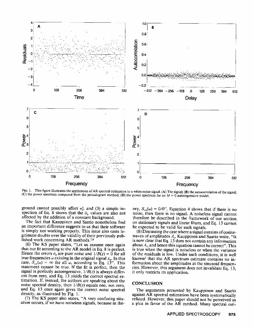
At this point, we wish to present a similar example of our own. A normally distributed random number generator is used to generate 512 observations. The mean of these observations is then computed and subtracted from each observation--a process equivalent to performing an autoregression of order 0. These data are plotted in Fig. 1A, and their autocorrelation spectrum in Fig. 1B. It can be seen that the autocorrelation is not significantly different from a Dirac delta function, as required by Eq. 3; i.e., that the assumption that pi = 0 cannot be rejected at the 1% level, Vi 4= 0. This point shows that the white- noise assumption is valid for this sample, as expected. Figure 1C shows the spectral density of the data, as computed from the periodogram technique; the spectrum is indeed far from being flat. If the power spectrum is instead estimated from Eq. 13, we have for a white noise

ak = O, Vk > 0 (15) and, consequently,

Sxx = a~ = 1. (16)

If, instead, Eq. 14 is used to estimate Sxx(w), we have to determine which value of M yields a correct autoregressive model for the data of Fig. 1A. From Fig. 1B and Eq. 15, it is quite obvious that this correct value is M = 0. Equation 14 then gives

s~ S~,(w) = - f = 1.012 (17)

corresponding to the constant spectrum shown in Fig. 1D. This is of course very close to the "true" spectrum and illustrates one case where AR spectral estimation is far superior to periodograms.

Figure 2 of Ref. 1 shows a very bad result obtained by using AR spectral estimation. Here, the problem probably lies in the value used for M. Although there are no definite rules to find the best value for M, it is generally considered that M should be much lower than N, the number of points in the signal. In this example (and also the next one) the KS approach uses N = 120 and M = 110, i.e., values for which the method cannot be expected to yield good results. For this reason, we believe that these two examples bear no demonstrative value.

The last example, figure 3 of Ref. 1, is even more trou- bling. It first shows one signal treated by AR that yields a very bad spectrum. Then, by adding a constant background to the same signal, the authors show that the spectrum is much improved. This reasoning is of concern because it should be quite obvious that AR spectral estimation is invariant to the addition of a constant background. This point is readily shown by considering that (1) Eq. 13 states that the signal power estimate depends only on a~ and &k; (2) the addition of a constant back-

974 Volume 48, Number 8, 1994

4 1.0 A

3

2

1

o

0 : - 1

-2

: . ; . .

. . .. ~ • ~.. ". :'.;:. . ; . . . . . . . " : : : " .. . . ' , . " . . ' . . . . . , ' . . . . ' . . "

• . ' . " . 7 . ". " "~ . . . . . . : ' ' : . . .

, . . . • . • , . :

• . : , . ,

-3

- 4 . . . . . . . . ~ _ _

0 128 256 384 512

Time

0.8

c .O 0.6

"~ 0.4

O "~ 0.2 <

0.0

-0.2

-512 - 3 ~ -256 -128 0

.. . . . . :~ . . . . . . . . . , . = .'~:~. :':~.:... .~:'~ ..::... : . . . . . . . . . : . . .

. . . . • " . . : • . . ' : ' , ' V q . " : : . ' , ' . ; , : . ~ t , . ' ~ : : : ~ o ~ ' . . : , ~ : r ~ : . " " M ~ ' : ' . : " ~ " : . " . "~" = " " "

. . . . . r . . . . . ~ ~ 7

128 256 384 512

Delay !I

2

1

0

C

• " . ~ • • .

i

7

6

5

2

1

0 0 0 128 256 384 512 128 266 384 512

Frequency Frequency FIo. 1. This figure illustrates the application of AR spectral estimation to a white-noise signal. (A) The signal; (B) the autocorrelation of the signal; (C) the power spectrum computed from the pefiodogram method; (D) the power spectrum for an M = 0 autoregressive model.

ground cannot possibly affect atE; and (3) a simple in- spection of Eq. 8 shows that the 3k values are also not affected by the addition of a constant background.

The fact that Kauppinen and Sarrio nonetheless find an important difference suggests to us that their software is simply not working properly. This issue also casts le- gitimate doubts over the validity of their previously published work concerning AR methods. 7,8

(6) The KS paper states, "Let us assume once again that our fit according to the AR model in Eq. 8 is perfect. Hence the errors e, are pure noise and 1 / B ( z ) = 0 for all true frequencies ~ existing in the original signal x,. In this case, S~(o~) = oo for all ~, according to Eq. 13". This statement cannot be true. If the fit is perfect, then the signal is perfectly autoregressive, I / B ( z ) is always different from zero, and Eq. 13 yields the correct spectral estimation. If, instead, the authors are speaking about the noise spectral density, then 1 / B ( z ) equals one, not zero, and Eq. 13 once again gives the correct noise spectral density, as illustrated by Fig. 1.

(7) The KS paper also states, "A very confusing situ- ation occurs, if we have noiseless signals, because in the-

ory, Sxx(o~) = 0/0". Equation 4 shows that if there is no noise, then there is no signal. A noiseless signal cannot therefore be described in the framework of our section on stationary signals and linear filters, and Eq. 13 cannot be expected to be valid for such signals.

(8) Discussing the case where a signal consists of cosine- waves of amplitudes Ai, Kauppinen and Saario write, "It is now clear that Eq. 13 does not contain any information about A i , and hence this equation cannot be correct". This is true when the signal is noiseless or when the variance of the residuals is low. Under such conditions, it is well known 3 that the AR spectrum estimate contains no information about the amplitudes at the sinusoid frequencies. However, this argument does not invalidate Eq. 13, it only restricts its application.

CONCLUSION

The arguments presented by Kauppinen and Saario against AR spectral estimation have been systematically refuted. However, this paper should not be perceived as a plea in favor of the AR method. Many spectral esti-

APPLIED SPECTROSCOPY 975

mation methods exist, each presenting its advantages and pitfalls; none of these should be regarded as a universal method for solving all problems.

In the case of AR spectral estimation, one should first make sure that there are physical reasons to assume that the signal is autoregressive. Then, proper statistical tests should be performed to assess the validity of the autoregression. Finally, if the S/N ratio is not too high, one can feel confident about the validity of the spectral estimation.

ACKNOWLEDGMENT

The authors wish to thank Prof. J.-P. Rasson for careful reading of the manuscript.

1. J. K. Kauppinen and E. K. Saario, Appl. Spectrosc. 47, 1123 (1993). 2. G. P. Box and G. M. Jenkins, Time Series Analysis Forecasting and

Control (Holden-Day, New York, 1970). 3. S. J. Orfanidis, Optimum Signal Processing." An Introduction (Mac-

Millan, New York, 1988), 2nd ed. 4. A. Papoulis, IEEE Trans. Acoust., Speech, Signal Processing, ASSP-

33, 933 (1985). 5. P. Whittle, Prediction and Regulation (Van Nostrand Reinhold, New

York, 1963). 6. G. Leclerc and J. J. Pireaux, paper submitted to J. Electron. Spec-

trosc. Relat. Phenom. (1993). 7. J. K. Kauppinen, D. J. Moffatt, M. R. Holberg, and H. H. Mantsch,

Appl. Spectrosc. 45, 411 (1991). 8. J. K. Kauppinen, D. J. Moffatt, and H. H. Mantsch, Can. J. Chem.

70, 2887 (1992).

976 Volume 48, Number 8, 1994

Documents

What Is Wrong with "What Is Wrong with MEM?"