What Prevents Female Executives from Reaching the Top?*

Matti Keloharju

Aalto University School of Business, CEPR, and IFN

Samuli Knüpfer

BI Norwegian Business School and IFN

Joacim Tåg

Research Institute of Industrial Economics (IFN)

December 15, 2017

Abstract

Exceptionally rich data from Sweden makes it possible to study the gender gap in executives’ career progression and to investigate its causes. In their forties, female executives are about one-half as likely to be large-company CEOs and about one-third less likely to be high earners than males. Abilities, skills, and education likely do not explain these gaps because female executives appear better qualified than males. Instead, slow career progression in the five years after the first childbirth explains most of the female disadvantage. During this period, female executives work on average shorter hours than males and are more often absent from work. These results suggest that aspiring women may not reach the executive suite without trading off family life. JEL-classification: G34; J16; J24; J31

* E-mails: matti.keloharju@aalto.fi, samuli.knupfer@bi.no, joacim.tag@ifn.se. We thank Espen Eckbo, Robert

Fairlie, Claudia Goldin, Lena Hensvik, Arizo Karimi, Victor Lavy, Johanna Rickne, Martin Olsson, Matti Sarvimäki, Claudia Olivetti, Margarita Tsoutsoura, Karin Thorburn, Luigi Zingales, and seminar participants at BI Norwegian Business School, Boston College, Boston University, City University London, Harvard Business School, Hong Kong Baptist University, Hong Kong University, IFN, Linnaeus University, Northeastern University, Norwegian School of Economics, Stockholm School of Economics, Stockholm University, University of Bristol, University of Exeter, University of Massachusetts at Boston, University of St. Gallen, Uppsala University, and in the National Conference for Swedish Economists for valuable comments and suggestions, and the Academy of Finland, Deloitte Institute of Innovation and Entrepreneurship, and Marianne and Marcus Wallenberg Foundation for financial support. Simon Ek, Charlotta Olofsson, and Ingvar Ziemann provided excellent research assistance. This paper replaces our earlier working paper entitled “Equal Opportunity? Gender Gaps in CEO Appointments and Executive Pay”.

1

1. Introduction

Women are less represented in the upper echelons of corporations than men. In S&P 500

companies, women account for 45% of the work force but hold only 27% of the executive and

senior-level official and manager positions. The fraction of women is even smaller at the very top

of the organization: women account for 5% of the CEO positions (Catalyst 2017). And when women

are appointed to top executive positions, they tend to earn less than men. Bertrand and Hallock

(2001) find that women earn 45% less than men among the highest-paid corporate executives.1 What

explains these patterns?

Some argue that women are disadvantaged compared to men when it comes to leading

corporations. Their preferences might make them shy away from competitive and risky

environments.2 The investments they have made to human capital and the career paths they have

chosen might make them poorly equipped to reach the top.3 Time spent with children can lead them

to miss valuable opportunities, and standing by the family may prevent them being available when

the firm needs them most.4

1 Albanesi, Olivetti, and Prados (2015) find significant gender differences in the structure of executive pay, which

exposes female executives’ earnings more to bad firm performance. Albrecht, Björklund, and Vroman (2003) and Boschini, Gunnarsson, and Roine (2017) document that gender gaps are particularly large at the top of the wage distribution. Blau and Kahn (2000, 2017) and Goldin (2014) offer reviews of the gender differences in pay.

2 See, for example, Croson and Gneezy (2009), Bertrand (2011), and Niederle (2016) for reviews of the gender differences in preferences.

3 Bertrand et al. (2010) show that female MBA students are less likely than men to take finance courses. Because of the large returns to finance education, this selection contributes to the gender gap in earnings.

4 Bertrand et al. (2010) and Azmat and Ferrer (2017) document that male MBAs and lawyers work longer hours than their female peers.

2

Others argue that the lack of women in top positions reflects negative stereotypes that hamper

the rise of females on the corporate ladder.5 One version of this argument appeals to the fact that

women who have made it to the executive level (and are potentially just one step from the CEO

position) are a highly selective group of individuals.6 Their career success constitutes direct

evidence of their talent, skills, and ambitions, and the income and career prospects that come with

this success mean that their opportunity costs of dropping out of the labor force or reducing work

hours to care for children are exceptionally high (Adams and Funk, 2012, Wood et al., 1993). These

considerations speak against the possibility that there would be substantial performance differences

between male and female executives. The large gender differences in career progression and pay

documented in the literature would thus be more likely an outcome of negative stereotyping than of

gender-related performance differences.7

Using comprehensive data on top executives of Swedish firms, we evaluate the merits of these

explanations. We follow the careers of all future executives born between 1962 and 1971 in the

1990–2011 period and ask how their qualifications, career progression, and family matters explain

their career success in 2011, i.e. when they are in their forties. Our data cover the entire adult

population of Sweden and all its firms, including private ones, resulting in an exceptionally large

sample. We collect a comprehensive battery of characteristics of the executives and their family and

relatives, which allows us to analyze a host of gender differences, including those related to child

5 Becker (1959) analyzes taste-based discrimination whereas Phelps (1972) and Arrow (1973) study statistical

discrimination based on characteristics of the average member of a group. Taste-based discrimination models predict that greater competition between employers will reduce discrimination. Consistent with this idea, Heyman, Norbäck, and Persson (2017) find a negative association between product market competition and gender gaps in managerial appointments and pay.

6 See Adams and Funk (2012) for a similar argument for board members. 7 In some countries, policy makers have imposed quotas to balance the outcome differences between genders. Ahern

and Dittmar (2012), Bertrand et al. (2014), Eckbo, Nygaard, and Thorburn (2016), Bagues and Campa (2017), Besley et al. (2017), and Tyrefors Hinnerich and Jansson (2017) study the effects of imposing gender quotas in business and in politics.

3

rearing and preferences. We complement the data set with survey responses on the time use of

executives in 2000–15. Almost all of our data come from official government registries and thus are

likely more reliable than the biographical and self-reported data used by many studies on top

executives.

We find that family matters play a crucial role in the formation of gender gaps. The gender

gaps in top executive appointments arise primarily during the five years following the birth of the

first child. During this period, female executives work on average shorter hours than male executives

and are more often absent from work. Women are on similar career paths as men prior to childbirth

but they earn substantially less than men five years after childbirth. This gender difference persists

over the remaining course of the executives’ careers.

Our results are consistent with family life putting a disproportionate burden on the careers of

women. Female executives are less likely to marry than male executives, and their marriages end

more often in divorce. They are less likely to have children and have on average fewer children.

They may also not be in a position to put their own career first: their partners tend to have higher

career and earnings potential than the partners of male executives.

We also analyze the extent to which the gender gaps at age 40–49 can be accounted for by other

characteristics of the executives. Our specifications suggest that a labor market that treats the basket

of attributes of each executive without regard to gender would generate a gender gap of the opposite

sign than that observed in the data. For example, female executives tend to have much higher levels

of education, which is one of the strongest predictors of making it to the top. They are more likely

to receive their degrees from tracks that produce a large number of top executives. They have

worked in a larger number of firms and are more likely to have acquired experience from consulting

or investment banking, an indication of their taste for competition and willingness to work long

hours. Their male siblings also attain higher cognitive ability test scores in the military enlistment.

4

These differences in qualifications go against the idea that female executives lack the necessary

skills, training, and stamina to make it to the top. The higher female bar for reaching the top suggests

instead that aspiring women may have invested more in their basket of qualifications to prevent the

adverse effects of child rearing.

To achieve a homogenous sample, we focus on individuals who have made it to the executive

level. The ex post success of the women in our sample means that their career setbacks due to

childbirth can be expected to be smaller and of more temporary nature than those of talented women

on average. To check the extent to which our results generalize to other talented professionals, we

replicate our most important analyses for a sample of business, economics, and engineering

graduates—the three most common fields of education for corporate executives—relaxing the

requirement of an individual holding an executive position at the end of the sample period. We find

that female university graduates enjoy a smaller qualification advantage over men than executives,

because sample selection strips women of one of their key strengths: their higher level of education.

This helps explain why the gender gaps in top executive appointments are as much as one-third

larger in the university graduate sample than in the executive sample. In both samples, income

development during the five years after first childbirth accounts for about three-quarters of the

gender gaps in top executive appointments. Thus, selecting the sample based on ex post career

success does not seem to have a tangible effect on how informative the setbacks due to childbirth

are of long-term career outcomes.

Our paper contributes to the literature on gender differences in labor market outcomes, in

particular at the top level of organizations, in the following ways. First, we are to our knowledge

5

the first to analyze gender gaps among top executives using data on their careers.8 Combining career

information with data on childrearing allows us to identify the effect of family on an executive’s

career trajectory and later gender gaps. Information on working hours and absence from work

provide evidence on underlying mechanisms. The focus on executives, whose career aspirations

may make them willing to invest in easing the burden of child rearing, speaks to understanding how

binding the family constraints are for the population at large. Adda, Dustmann, and Stevens (2017),

Angelov, Johansson, and Lindahl (2016), and Kleven, Landais, and Søgaard (2017) analyze the

impact of child rearing on the population gender gap. Second, we document gender differences in

executive characteristics in much more detail than the previous literature and can directly address

the assumption that male and female executives hold similar qualifications. Our exceptionally large

battery of variables not only allows us to gain more insight into the differences between male and

female executives, but also allows us to gain a better understanding of how various characteristics

contribute to the gender gaps. Our result that female executives are more qualified than males and

that these qualifications generate a counterfactual female advantage over males in executive

appointments adds a new dimension to the literature.

Our paper proceeds as follows. The next section describes the data and the institutional setting.

Section 3 analyzes gender differences in executives’ qualifications and the extent to which these

differences can explain differences in career outcomes. Section 4 studies gender differences in

executives’ family life and their contribution to working hours, absence from work, early career

development, and later career outcomes. Section 5 concludes.

8 Smith, Smith, and Verner (2013) study gender differences in CEO appointments in Denmark, but do not follow

executives’ careers over time. Matsa and Miller (2011) focus on the role of female board representation in CEO appointment decisions. Bertrand, Goldin, and Katz (2010), Azmat and Ferrer (2017), and Kunze and Miller (2017) use career data on professionals but not on top executives.

6

2. Data and institutional setting

2.1. Data

2.1.1. Main sample

The sample consists of all individuals born between 1962 and 1971 who worked in 2011 as an

executive in a Swedish limited-liability company with at least 10 employees and information on

sales available. We follow the careers of these individuals in the 1990–2011 period and ask how

their qualifications, career progression, and family matters explain their career success in 2011, i.e.

when they are in their forties. For executives with children, we require that the first child was born

in 1992–2001, i.e. 10–19 years (on average, 15 years) before the time when we assess their career

success. Executives that have no children enter the sample if their imputed childbirth, which we

assign based on the observed distribution of age at first childbirth, is in 1992–2001. These criteria

trade off the sample subjects having made significant progress in their careers against our ability to

observe their first childbirth. The average 15-year follow-up period following the first childbirth

further avoids mixing temporary career setbacks due to small children with long-term career

outcomes. Our data set combines information on individuals and firms from three sources.9

Statistics Sweden. The bulk of these data come from the LISA database that covers the whole

Swedish population of individuals who are at least 16 years old and resident in Sweden at the end

of each year. This database integrates information from registers held by various government

authorities and covers for most variables the years 1990–2011. We extract information on labor and

total income, field and level of education, profession, career, and family relationships. The family

9 The sensitive nature of the data necessitated an approval from the Ethical Review Board in Sweden and a data

secrecy clearance from Statistics Sweden. The identifiers for individuals, firms, and other statistical units were replaced by anonymized identifiers and the key that links the anonymized identifier to the real identifiers was destroyed. The data are used through Microdata Online Access service provided by Statistics Sweden.

7

records allow us to map each individual to their spouses, children, parents, and siblings. We use

information on the brothers of the executives to impute variables that are not observable for the

executives themselves or that may be contaminated by gender (for example, school GPAs may

reflect gender-biased grading). Except for the CEOs, whom Statistics Sweden separately classifies,

we identify the executives based on their international ISCO-88 (COM) classification of

occupations (codes 122 and 123).10 The specialist managers further split into eight functions that

include finance and administration, personnel and industrial relations, sales and marketing,

advertising and public relations, supply and distribution, computing services, research and

development, and specialists not classified to the above categories.

The Swedish Companies Registration Office. The Swedish Companies Registration Office

keeps track of all companies, both public and private, and their CEOs and directors. The firm data

are available for all corporate entities that have a limited liability structure (“aktiebolag”) and that

have appointed a CEO (“verkställande direktör”), excluding financial firms that operate as banks or

insurance companies. These data record various financial statement items, including sales and the

number of employees. By law, each firm has to supply this information to the registration office

within seven months from the end of the fiscal year. Financial penalties and the threat of forced

liquidation discourage late filing.

10 The ISCO-88 (COM) code 122 corresponds to ”production and operations managers” and the code 123 to ”other

specialist managers.” The occupation data available from the LISA database come mainly from the official wage statistics survey (Lönestrukturstatistiken). Statistics Sweden also undertakes surveys of smaller firms (primarily with 2–19 employees) that are not included in the official wage survey. The sampling design in the supplementary surveys is a rolling panel and all eligible firms are surveyed at least once every five years. Occupation information is available for each year, but the information may not be accurate for each year. To ensure that we have accurate occupation information for every year, we require that the information be collected in the relevant year or earlier and for the correct employer-employee link. Andersson and Andersson (2012) describe how Statistics Sweden identifies operative CEOs of firms. If an individual holds multiple executive positions, we assign the individual to the executive position in the firm with the highest sales.

8

Military Archives. The Military Archives stores information on the service record, the health

status, and the cognitive, non-cognitive, and physical characteristics of all conscripts. The purpose

of the data collection is to assess whether conscripts are physically and mentally fit to serve in the

military and suitable for training for leadership or specialist positions. The examination spans two

days and takes place at age 18. Lindqvist and Vestman (2011) offer a comprehensive description of

the testing procedure. These data are available for Swedish males drafted in 1970–1996. Military

service was mandatory in Sweden during this period, so the test pool includes virtually all Swedish

men born between 1951−1978.

Our main sample encompasses over 24,000 executives. Given the sample size, most of our

results are highly significant. Therefore, our reporting generally focuses on coefficient values and

patterns rather than on their statistical significance.

2.1.2. Additional and alternative samples

In addition to our main sample, we study the time use of 9,300 corporate executives as

measured by the Labour Force Survey in 2000–15. The survey asks a randomly selected sample of

respondents to report on the number of hours worked, contracted, and absent in the week preceding

the survey. We merge the survey responses with administrative data from the LISA database on the

number of days in which the respondent has claimed compensation for absence due to parental

reasons, and on selected socioeconomic characteristics. Among these characteristics is information

on the number of children in various age categories for each executive. Our Labour Force Survey

sample does not link to the core executive sample, so we cannot track the Labor Force Survey

executives before or after the survey.

We complement our analysis of future executives with an analysis of university graduates. We

construct this sample using the selection criteria for the core executive sample except for requiring

9

each individual to hold a degree from business, economics, or engineering, and relaxing the

requirement of an individual holding an executive position in 2011.

2.2. Childcare system in Sweden

Sweden has a high-quality childcare system that has been in place from the mid-1960s. It

guarantees each family twelve months of publicly paid parental leave amounting usually to 75% of

prior income (before 1995, 90% of prior income), with an option of extending the leave with three

months at a lower rate. Parents can use up to 90 days per year with publicly financed paid leave for

care of a sick child, and they have the option of working shorter hours while keeping their full-time

job. Since 1995, both parents need to take one month of parental leave to qualify for the maximum

paid leave. This “daddy month” increased the use of paid parental leave by fathers, but reduced the

use of the unpaid part, leading only to minor effects on labor supply (Ekberg et al. 2013). Day care

is available at highly subsidized rates, although its service hours make it less flexible than the day

care in the U.S. (Henrekson and Stenkula, 2009).

3. How do female executives differ from males?

3.1. Gender gaps in top executive appointments

Table 1 Panel A characterizes the career progression of female and male executives by focusing

on top executive roles. We define these roles in three different yet overlapping ways, utilizing

information on the executives’ formal roles and on their pay. The three leftmost column report on

those executives who have become CEOs of large companies, defined here as companies with sales

of at least SEK 500 million (SEK 1 ≈ USD 0.12). 0.77% of female executives make it this far, while

the corresponding fraction among male executives is 1.41%. Despite of a relatively small number

10

of top-executive observations (there are 300 large-company CEOs, of whom 51 are women), the

gender gap in the likelihood to attain a top position, −0.64 (= 0.77 − 1.41), is statistically highly

significant with a t-value of –4.6. This gap reflects the fact women account for 17% large-firm CEOs

as opposed to 27% of the executives in the full sample. The three middle columns represent a

broader definition of large-firm top executives that adds the four highest paid non-CEO executives.

This group of people would typically coincide with the company’s top management team. Women

account for 21% of this group of executives, i.e. the gender gap is relatively smaller among large-

firm top executives than among CEOs. Finally, the three columns on the right report on an even

broader definition of a top executive that does not explicitly factor in firm size but focuses on pay

instead. The cutoff for a top executive here is having a labor income of at least SEK 1 million, which

roughly corresponds to the top decile in pay among all executives in Sweden. The fraction of women

in this group is 20%, i.e. about the same as among large-firm top executives.

Table 1 Panel B reports the mean and median executive labor income by gender and position.

Our income measure includes all income taxed as labor income in a given year; base salaries, stock

option grants, bonus payments, and benefits received from the employer qualify as taxable labor

income. The income measure does not include public benefits, providing a better proxy of the value

of an executive’s services to the company than a broader income measure. Tax authorities deem the

taxable income to occur in the year when an employee or executive exercises her stock options or

purchases her company’s shares at a price that is less than their fair value.

The mean (median) large-firm CEO pay is SEK 2.1 million (1.7 million). On average, the

sample executives make about one third, and large-firm executives about two thirds, of what large-

firm CEOs make. Executive men earn more than women, but the pay gap is relatively small. For the

top executive categories, the mean logged pay gap ranges from –3% (large-firm CEOs and highly

paid executives) to –9% (large-firm top executives).

11

Table IA1 in the Internet appendix reports descriptive statistics on the 11,063 sample

companies. The mean sales are SEK 385 million and the mean number of employees is 126. The

vast majority of the firms are privately held: only 1% are listed and 4% government owned.

3.2. Gender differences in executives’ education, career, family background, and traits

Table 2 reports the means of all individual-level variables, separately for women, men, and the

full sample. Of particular interest is the difference between women and men and the t-statistic for

their difference. We report on 56 variables divided into nine different groups. 21 of the variables

are continuous and 35 dummy variables. We use these variables in regressions as such except for

the dummies on the level and field of education and the executive functions, where we drop one of

them. The variables for the first seven groups—level of education, educational specialization, career

orientation and networks, career, functional experience, family background, and risk tolerance—are

available for all sample subjects and are reported on in Panel A, B, C, and D. Panel E reports on the

remaining two groups of variables, parents’ socioeconomic status and personal traits. They are

available only for subsets of the sample and are reported as robustness checks (availability of

parental variables depends on the parent being alive in 1990 and the personal traits can be imputed

for executives whose brothers were enlisted to the military in 1970–1996).

Panel A reports on gender differences in the level of education, a classic predictor of pay

(Mincer, 1958). We find that 48% of female corporate executives hold a degree from a university,

while the corresponding fraction for men is 30%. Correspondingly, men are more likely to belong

to any of the lower education level categories. For example, men are more than twice as likely as

women to have an education level lower than high school.

12

Panel A further reports on the field of education, which measures differences in executives’

skill sets and their propensity to specialize and remain specialists through their executive careers.11

The field of education also correlates with competitiveness, in which there are large gender

differences (Gneezy et al., 2003 and Niederle and Westerlund, 2007). Buser, Niederle, and

Oosterbeck (2014) find that competitive individuals are more likely to select the most prestigious

study tracks, which tend to include more math and science classes. Kamas and Preston (2015) find

that competitive individuals are more likely to specialize in engineering, natural sciences, and

business as opposed to majoring in social sciences or the humanities. We find that men are much

more likely to have an engineering degree (52% vs. 16%), while women are more likely to have a

degree from all other backgrounds. For example, the fraction of female executives with a business

degree is 43%, while the corresponding fraction for men is 24%.

Panel B finds that women are more likely to have chosen one of the top-5 education tracks (top-

5 high schools) that produce the highest proportion (number) of large-firm top executives. Attending

these education tracks may help build careers through better networks: Hwang and Kim (2009),

Kramarz and Thesmar (2013), and Engelberg, Gao, and Parsons (2013) report evidence of the

usefulness of networks for executive careers. In addition, these education tracks may reveal

executives’ career orientation and inform of their competitiveness. Despite of their greater

likelihood of attending network-rich education tracks, female executives are less likely to select into

the top-5 education tracks offering the highest income.

Panel B further studies gender differences in careers. The executives are on average 44 years

old. Men are on average 0.3 years older than women but have two years longer labor market

11 The opposite of becoming a specialist is to become a generalist, a job description commonly associated with CEOs.

Murphy and Zábojník (2004) and Custódio, Ferreira, and Matos (2013) analyze generalist CEOs.

13

experience. The fact that the gap in work experience is larger than the age gap is consistent with the

idea that men have experienced fewer career interruptions than women. Despite of their shorter

career, women have experience from more companies and from more industries than men. This

more varied experience helps build women’s general human capital, while men’s longer tenure in

the firm helps build their firm-specific human capital.

Panel B also suggests that men and women have different work experience. On the one hand,

women have on average longer work experience from consulting and investment banking. Both

industries frequently use of tournament-type (“up or out”) promotion structures and likely attract

competitive individuals. Such experiences may also be valuable in building networks and acquiring

generalist skills. On the other hand, women also have more experience from non-profit institutions.

Work experience from a non-profit organization may accumulate a future executive’s human capital

in a different way than work experience from a company. In addition, working for not-for-profit

firms or for the public sector may be an indication of altruistic preferences (Benz 2005 and

Delfgaauw and Dur 2008), of which there is some evidence of gender differences.12

Finally, Panel B studies gender differences in unemployment. Male executives have on average

23 days less unemployment experience than female executives. This difference may matter because

unemployed individuals may lose some of the value of their human capital due to unemployment

(Pissarides (1992)), or be scarred by the unemployment experience (Arulampalam (2001)). The fact

that female executives are more likely to have graduated during a recession may partly explain the

difference in unemployment experience. Oyer (2008), Custódio, Ferreira, and Matos (2013), and

12 Women are sometimes assumed to be more altruistic and cooperative than men. Niederle (2016) reviews the

experimental and field evidence on altruism and cooperation and concludes that the evidence “is more mixed than what one might have expected.”

14

Schoar and Zuo (2017) find that starting a career at the time of a recession has a lasting impact on

career success and pay.

Panel C reports on gender differences in past work experience in different executive functions.

Given that specialization in a given function is likely to require a considerable human capital

investment, past functional experience is likely to affect future executive assignments (in anecdotal

accounts of gender gaps in business, this explanation is referred to as the pipeline hypothesis).

Women outnumber men in finance and administration, personnel and industrial relations, and

advertising and public relations.

Panel D reports on gender differences in family backgrounds. There are relatively small

differences between male and female executives in their birth order, family size, number of male

siblings, immigrant status, or whether they were born in a large city. The most important difference

in background relates to female executives having a smaller propensity to work in their birth county

(42% vs. 49%). Figure IA1 shows that the gender gap in executives’ likelihood to live in their home

county becomes apparent already in the early 20s when they typically study at college. These results

are consistent with the idea that female executives are, if anything, more prone than male executives

to move to opportunity.

Panel D further reports gender differences in risk tolerance, which we measure by using an

indicator as to whether the executive is a stock market participant. Jianakoplos and Bernasek (1998)

and Sunden and Surette (1998) document that women typically hold lower proportions of risky

assets than men. Reviews by Eckel and Grossman (2008) and Croson and Gneezy (2009) of the

experimental literature come to the same conclusion: women tend to be more risk averse than men.

Our results support the findings in this literature: 50% of women own stocks, while the

corresponding fraction for men is 65%. These findings are at odds with the findings of Adams and

Funk (2012), which suggest that female directors are more risk tolerant than male directors.

15

Panel E reports gender differences in variables that are not available for the entire sample. We

first report on parents’ socioeconomic status. Being born to a well-educated and affluent family can

help a child in at least two ways. First, parents are likely to pass their human capital on to their

children. Second, wealthy parents are also in a better position to offer the monetary resources needed

to develop their children’s human capital. We separately include both parents’ socioeconomic status

by including variables measuring whether they are (or were) university educated. We also measure

their employment in 1990 (i.e. at the beginning of our sample period) and their position in the

income distribution among individuals of the same gender and cohort. We find that female

executives appear to come from higher socioeconomic strata than male executives. Female

executives’ both parents are on average better educated and have higher earnings.

Panel E also reports on personal traits. Swedish military measures all personal trait variables,

except for GPA. Military service is mandatory only for men, so we have very few traits observations

for women. Nevertheless, the family links in our data make it possible to impute these variables for

an executive from the test scores of her randomly selected brother (we randomly choose just one

brother to avoid biases arising from family size). This imputation assumes that the traits have a large

family component, an assumption backed up by the evidence in Beauchamp et al. (2011) in Swedish

data. We also impute the traits for men even though their traits are available.13 Given that executives

have done well in life, their traits likely are better than those of their brothers. Except for imputed

officer rank, we express all trait variables as differences in terms of standard deviations relative to

the test takers in the same cohort. Benchmarking each individual against the same cohort allows us

13 Table IA2 investigates the possibility that the imputation picks up women and men executives from families of

different socioeconomic status, perhaps because of cross-sectional differences in parents’ desire to balance their family’s sex composition. The table shows no significant differences in parents’ socioeconomic status by imputation status and gender.

16

to control for secular trends in measured cognitive ability and height (see, e.g. Flynn (1984) and

Floud, Wachter, and Gregory (1990)).

We find that all trait variables except for the body mass index are positive. This means that the

brothers of executives have a higher cognitive and non-cognitive ability, are taller, slimmer, and in

better physical condition than the population. Consistent with Adams, Keloharju and Knüpfer

(2017), which reviews this literature, the differences relative to the population are relatively small,

at most 0.36 standard deviations. Four gender differences are statistically significant at the 1% level.

Women’s brothers have a higher cognitive ability (0.14 standard deviation difference), are slimmer

(0.08 standard deviation difference), and they are more likely to have achieved an officer rank than

men’s brothers. In addition, women’s brothers have a 0.08 standard deviations higher GPA than

men’s brothers. We use imputed GPAs to account for potential gender differences in grading.

3.3. Contribution of executive characteristics to gender gaps in executive appointments

Table 3 evaluates how much of the gender gap in large-firm top executive appointments and

pay can be attributed to gender differences in the executives’ characteristics. The three leftmost

columns of Table 3 Panel A report results from linear probability model regressions of the large-

firm CEO dummy on female dummy and controls. The first row represents a regression that includes

female dummy as the sole regressor. This regression corresponds to Table 1 that finds a coefficient

on the female dummy of –0.64. The second row reports regressions that also control for the level

and field of education. Given that women have on average better educational qualifications, the

gender gap widens to –1.06. Adding career orientation and networks and career controls on the third

row results in a gap of –0.98. Here, we use all the variables listed in Table 2 Panel B except for age,

which is highly correlated with the length of labor market experience. The fourth row adds dummies

for past functional experience, which lowers the gap to –0.88. And finally, the fifth row adds family

17

background and risk tolerance variables, bringing the gap to –0.75, i.e. relatively close to the

unconditional gap in the first specification.

The three rightmost columns report on regressions where the left-hand side variable is a dummy

for earning at least one million SEK. The unconditional probability for an executive to reach this

income is higher than that for being a large-firm CEO, 13.0% vs. 1.2%. Here, the unconditional

gender gap coefficient is –4.7, i.e. the same as in Table 1. Like for CEOs, the gap widens to –8.7

once we control for education, and then narrows again when we control for the other attributes. In

the regression with all controls, the gap continues to be larger than the unconditional gap (–6.9).

The three columns in the middle, which look at large-firm top executives, mirror the patterns we

observe for the highly paid executives. Overall, all our results point towards the conclusion that the

gender gaps do not arise from female executives’ poorer qualifications. The higher female bar for

reaching the top suggests instead that aspiring females may invest more in their basket of qualifications

to prevent the adverse effects of child rearing.14

Panel B includes additional controls to the regression equation. Given that these regressors are

not available for all of the executives, the number of observations and the unconditional and

conditional gender gaps are different than in our main specification. We consider three groups of

variables: parents’ socioeconomic status, personal traits, and imputed GPA, which we include to the

regression one by one in addition to all the variables used in Panel A. We find that the gender gap

widens with all of these variable groups in all specifications. If anything, these results strengthen

our conclusion that the cumulative impact of all the characteristics we employ makes the gender

gaps in top executive appointments and pay larger than those observed in the data.

14 More generally, professionals facing greater barriers in their careers may need to outperform their peers to be

promoted. Chuprinin and Sosyura (2017) find that mutual fund managers originating from worse socioeconomic background deliver better performance than managers from better background.

18

Apart from the female dummy, the regression coefficients on the predictors of top executive

appointments and pay are of interest. Table 3 Panel C reports on the large-firm CEO, large-firm top

executive, and high-earner coefficients for the specification that includes controls for individual

characteristics.

The specifications on the three definitions of top executives largely agree on how the predictors

are associated with executives’ labor market success. The level of education has a positive and

significant relation both with all the three definitions of top executives. For example, executives

with a university degree are more likely to become large-firm CEOs and tend to be better paid, but

those with a degree in health, natural science, teaching, or services tend to be less well paid than the

executives on average (the omitted category are executives with no known specialization). More

career-oriented executives reach better labor market outcomes, as is witnessed by the large positive

coefficients for educational paths that are associated with high incomes. A longer labor market

experience and experience from a larger number of companies strongly positively relate with a

highly paid executive position, while longer unemployment spells negatively relate with labor

market success. Functional experience from sales and marketing has the strongest association with

high pay and future CEO appointments. Conditional on becoming executives and all the other

controls, immigrants do better than native Swedes on average. Finally, stock market participation is

strongly positively associated with executives’ job market success.

Table IA3 performs a decomposition exercise that allows us to assess the joint contribution of

all characteristics to executive gender gaps. This exercise offers identical estimates of unconditional

and conditional gaps as do the regression coefficients reported in Table 3, but it has the added benefit

of offering information on the contribution of each variable subset to the gap. We report both the

Blinder-Oaxaca (1973, 1973) and Fairlie (1999) decompositions. The former uses the linear

probability model whereas the latter takes into account the fact that the dependent variable is an

19

indicator. The decompositions reveal that risk tolerance, functional experience, and family

background help to explain the gaps whereas education, career orientation, and networks tend to

widen them. The gaps decompose similarly into explained and unexplained parts in the two

specifications, suggesting that our results are robust to using a logit specification instead of a linear

probability model.

4. Role of family life in explaining gender gaps in executive appointments

4.1. Gender differences in marital status and family formation

Table 4 reports on gender differences in family characteristics. Consistent with Folke and

Rickne (2016) who find that promotions increase the risk of divorce for women (but not for men),

female executives are more likely to be divorced than male executives. Female executives also are

less likely to have children than male executives, and they have fewer children. These results are

consistent with the idea that the executive role puts more strain on the family life of women than

men. As a general rule, these gender differences are higher for large-firm top executives and other

high earners. For example, the gender difference in the likelihood to be divorced is four percentage

points higher for the top executive categories than for executives in general.

4.2. Contribution of children to early career development

Figure 1 depicts the labor income development of executives from age 19 to 49 by gender. Both

genders start from about the same average annual income; at age 20, women even earn slightly more

than men. The incomes start to diverge noticeably in the late twenties, and by age 34 the average

pay difference reaches its peak, 127,000 SEK in favor of men. After that, the pay difference

decreases gradually, reaching 36,000 SEK (4%) at age 49.

20

The divergence in female and male pay coincides with the time people typically form their

families. This observation motivates an analysis that explicitly considers the impact of childbirth on

career progression of women and men. Figure 2 reports results from an event study that tracks

executives’ average annual labor income, labor force participation, and the probability of attaining

a new job relative to the birth year of the executive’s first child. For each of these outcome measures,

we separately compare women with children against men with children (labeled ‘Male benchmark’

in the graphs) and against women without children (‘Female benchmark’).15 When comparing

female executives against male executives, we regress the outcome variables on indicators for

females, each calendar year, each of the 15 years surrounding childbirth, and the interactions of the

female indicator and the years surrounding childbirth. The figure reports the coefficient estimates

along with their 95% confidence intervals for the interaction coefficients for each of the event years

except for year t – 5, which serves as the omitted category. When comparing female executives with

children against female executives without children, we replace the female indicator in the

regression with an indicator for whether the executive has children. Because executives who never

have children do not experience their first childbirth, we assign them an imputed childbirth by

randomly drawing from future executives’ observed age distribution within gender at first

childbirth. This makes it possible to isolate the impact of childbirth from other possible gender-

related income shocks that coincide with the typical timing of childbirth. The calendar year dummies

control for annual trends in the outcome variable. Kleven et al. (2017) uses a similar method to

estimate child penalties in the population of Danish workers.

15 See Waldfogel (1998), Miller (2011), and Kleven et al. (2017) for analyses on the pay difference between women

with and without children.

21

Figure 2 Panel A shows that labor income of men and women develops very similarly until

year t – 1. Then, in year 0, women’s salary drops 126,000 SEK below that of men, likely because

of reduced pay during the maternity leave. The drop continues to 171,000 SEK in year t + 1 because

of the uneven timing of childbirths throughout the calendar year. After picking up in year t + 2 up

to SEK 114,000, there is another drop in pay in year t + 3, to SEK 150,000. This drop appears to be

driven by the birth of a second child, which tends to happen two years after the birth of the first

child. Figure IA2 Panel A shows that female executives who only have one child do not experience

a pay drop in year t + 3. Female pay starts to noticeably recover in year t + 4. Despite of its

continuing recovery and higher growth rate compared to men, female executives’ income is still in

year t + 10 about 80,000 SEK lower than that of male executives.

Figure 2 Panel B illustrates the salary development of female executives with children using

female executives without children as the benchmark. The coefficient pattern is similar to that

reported in Panel A, except that women with children appear to be on a higher salary trajectory both

before the first childbirth and after year t + 4. Consistent with the better trajectory, Table IA4 finds

a significantly higher probability of becoming a top executive for female executives with children

than without children and that this difference is partly attributable to the better qualifications of

women with children. Low statistical power in some of the specifications in the table is a result of

a small number of observations in the top executive categories. As a whole, these results suggest

that if anything, female executives with children have higher qualifications than female executives

who do not have children. This makes it more difficult for us to reject the null hypothesis of no

outcome difference between these two groups after childbirth, and explains why the long-run child

penalty is smaller here than with the male benchmark.

22

Figure 2 panels C and D show that female executives’ labor market participation rate is, if

anything, greater than that of their benchmarks before first childbirth. After a plunge in years 0 and

t + 1, the participation rate recovers slowly and reaches the male participation rate in year t + 10.

Figure 2 panels E and F study the probability of attaining a new job around first childbirth.

Relative to their benchmark groups, female executives’ probability of attaining a new job decreases

significantly in year t – 1 (and further in year 0), suggesting that they plan the childbirth and take it

into account in their decision to search for a new job. The probability recovers quickly after that and

reaches the male benchmark in year t + 5.

To sum up, all panels in Figure 2 tell the same story: the careers of future female executives

tend to suffer at the time of childbirth, and it takes several years for them to recover from this career

shock. Table 5 demonstrates this result formally in a regression table, whose specifications

correspond to those of Figure 2 except for pooling the event years in four brackets (0–1, 2–5, and

6–10 years, and the omitted category of –5 – –1 years). Except for a dummy for 6–10 years in the

probability of attaining a new job specification, all of the post-birth variables are significantly

negative at the 5% level.

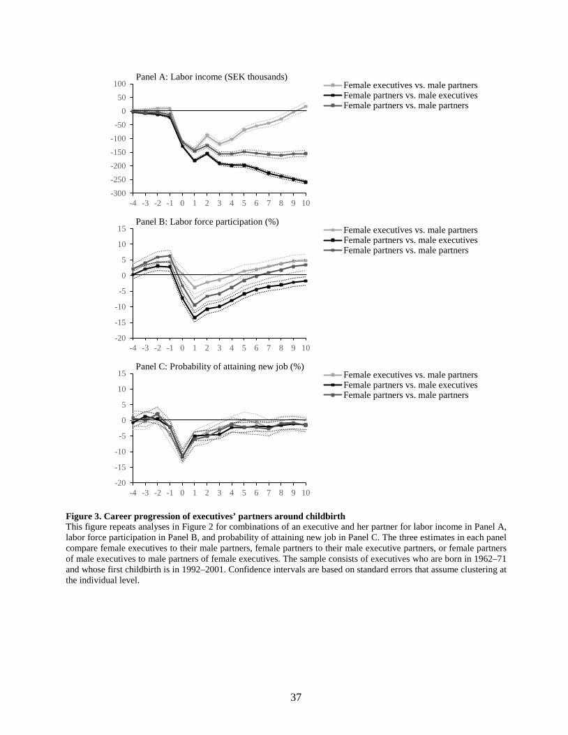
Figure 3 explores the role of the partners in sharing the responsibilities of child rearing by

comparing the career trajectories of the executives’ partners by gender. The female partners to male

executives assume a role very different from the male partners to female executives. Panel A

suggests that, compared to the male partners, female partners experience a permanent career setback

following childbirth. The magnitude of this penalty, SEK 143,000 in year t + 10, is almost twice as

large as the gender gap in pay for the executives themselves in Figure 2. Panel B shows that it takes

years until women’s labor market participation rates return to normal. Despite of starting from a

higher level, future female executives’ participation rate stays below that of their partners for four

years after childbirth. Female partners to male executives have a lower participation rate still in year

23

t + 10. Panel C shows that the gender gaps in the probability of attaining a new job are about the

same for all possible partner pairings. As in Figure 2, these gaps are large immediately after

childbirth (and a year before it) but largely disappear by year t + 5.

Table 6 reports on the characteristics of the executives’ partners. To gauge career pressure at

home, we calculate the predicted probability of being a top executive or a top earner for the

executive and the partner, separately for each gender. The predicted probability captures the effect

of all of our predictors known two years prior to first childbirth. The predicted probabilities are

higher for future executives than their partners, which is consistent with the idea that future

executives tend to “marry down” in a career sense. The likelihood of marrying down is slightly

higher for future male executives than for female executives. For example, 59.2% of executive

men’s partners have a lower probability to become CEO than the executive himself, while the

corresponding probability for executive women is 57.3%. The gender difference in the likelihood

to marry down is statistically significantly at the 5% level in two of the three specifications. The flip

side of this result is that female executives are more likely to belong to a dual-career family than

male executives. This may have an effect on their own careers as well.

4.3. Gender differences in working hours and absence from work

Why does childbirth have an asymmetric effect on the career outcomes of the two genders? One

plausible explanation for this asymmetry are gender differences in parental investment, which are

likely to be reflected in executives’ absence from work and in their working hours. We study these

differences by using a sample of executives surveyed by the Labour Force Survey in 2000–15.16 We

separately regress four absence and working hour variables on indicators for years 0, 1–2, 3–6, 7–

16 Table IA5 shows that these executives are broadly similar to our main sample executives in their characteristics.

Our survey sample includes a set of characteristics narrower than the core sample.

24

10, 11–16, and 17–18 years following childbirth (17–18 is the omitted category), a female indicator,

and their interactions, along with survey wave dummies. We report the coefficients for the

interactions along with their t-values (95% confidence intervals) in Table 7 (Figure 4).

The first specification in Table 7 (Panel A of Figure 4) reports on gender differences in the

annual number of days absent from work for parental reasons. In year 0, female executives are on

average 106 days more away from work for parental reasons than male executives. This gap narrows

as the children grow up, but it remains statistically significant at 6.6 days even 7–10 years after the

first childbirth.

The second specification (Panel B of Figure 4) reports on gender differences in weekly hours

absent from work. In year 0 female executives are on average 24 hours more absent from work than

their male counterparts. The gap drops to three hours in years 3–6 after first childbirth, and

disappears thereafter. The third specification (Panel C) shows that the gap in the number of working

hours follows a similar but reverse pattern. This gap stems from actual hours, not from contracted

hours. The fourth and final specification (Panel D) shows that the gender gap in contracted hours

does not differ statistically significantly in any of the years from the benchmark category of 17–18

years after childbirth.

These results suggest that female executives are more absent from work and work shorter hours

than male executives for many years after the birth of their first child. However, this gap largely

fades away by the time the first child reaches school age.

4.4. Impact of early career development on top executive appointments

The burden of child rearing on female careers motivates us to analyze how much of the

executive gender gaps at the age of 40–49 can be attributed to child rearing. Table 8 studies this

question by investigating the extent to which labor income five years after first childbirth—a direct

25

measure of the impact of children on career progression—explain the top executive gender gaps. In

this analysis, we separately account for labor income prior to childbirth, which captures other gender

differences in career development that do not arise from childrearing. We measure childbirths in the

1991–2000 period, i.e. on average 15 years before observing the top executive positions.

The three leftmost columns report the specification that explains appointments to a large-firm

CEO position. The first column serves as a benchmark and is identical to the specification with

controls listed on the fifth row of Table 3 Panel A. The gender gap here is –0.77. Column 2 asks

how the coefficient for the female dummy changes once we add income two years before the birth

of the first child.17 The gender gap decreases only slightly to –0.74, which is consistent with the

results in Figure 2 that show men and women are on similar career trajectories prior to first

childbirth. The income variable itself is highly significant, which implies strong persistence in the

career paths of aspiring executives.

Column 3 further adds income five years after first childbirth to the regression. The results in

Column 3 are strikingly different from those is Column 2. Now, both the female dummy and the

income one year before birth become insignificant, while the coefficient for income five years after

first childbirth takes a highly significant value. This result suggests that for large-firm CEO

appointments, the early career development in the five years following first childbirth accounts for

the entire gender gap.

We get qualitatively similar results also for the other top executive definitions. In the three

middle columns, where we regress appointment to one of the top-5 executive positions in large firms

on the female dummy and controls, the gender gap is –3.0 both in the baseline specification in

Column 4 and in Column 5 where we additionally control for income two years before first

17 We use income from year t – 2 in lieu of t – 1 to avoid any effects arising from pregnancy.

26

childbirth. In Column 6, where we further add income in year t + 5, the coefficient for the female

dummy drops to –1.3, while the coefficient for income in t + 5 is highly significant. Here, over one-

half (1 – –1.3/–3.0) of the gender gap can be accounted for by the income development during the

five years after first childbirth. This pattern repeats one more time in the three rightmost columns,

where we regress a highly paid executive dummy on the female dummy and controls. In Column 9,

which includes both income controls, we can account for 77% of the gender gap by the early career

development following first childbirth.

Table IA6 Panel A explores how doubling the total assets cutoff to SEK 1 billion and the pay

cutoff to SEK 2 million affect our results. The mean dependent variable at the bottom of the panel

shows the number of top executives drops approximately to one-half in the firm-size based

definitions (the six leftmost columns) and to one-sixth in the pay-based definition (the three

rightmost columns). The coefficient for the female dummy is negative and statistically significant

in all specifications before controlling for income in year t + 5, but becomes insignificant or even

reverses its sign once we add income in year t + 5.

Table IA6 Panel B explores robustness of our results in a sample of executives in their 50s. It

repeats the regressions in Table 8 but leaves out labor income at t – 2 as its measurement is not

possible prior to 1990. The results for this subsample are qualitatively similar to those for the main

sample. The coefficient for female dummy is statistically significantly negative in all specifications

before controlling for income, and it drops on average by more than one-half after controlling for

income in year t + 5. In other words, income five years after the childbirth accounts for more than

one-half of the gender gaps in top executive outcomes.

The ex post success of the women in our future executive sample means that their career

setbacks due to childbirth can be expected to be smaller and of more temporary nature than those of

talented women on average. To check how our results generalize to other talented professionals, we

27

analyze a sample of business, economics, and engineering graduates—the three most common fields

of education for corporate executives—relaxing the requirement of an individual holding an

executive position in 2011. Female university graduates enjoy a smaller qualification advantage

over men than executives, because sample selection strips women of one of their key strengths: their

higher level of education. This helps explain why the gender gaps are one-quarter to one-third higher

in the university graduate sample. For example, comparing Table 9 Panel A with Table 1 Panel A

suggests the fraction of women is one-third larger in the university graduate than in the executive

population, but about the same among large-firm CEOs. As shown by Table 9 Panel B, education

gives women an edge even in the university graduate sample, because they are more likely to have

a degree from business or economics, i.e. the fields of education most highly correlated with

appointment as a top executive.

Table 9 Panel C repeats the analyses of Table 8 using the university graduate sample. The

results of this analysis echo those of the main sample: on average about three-quarters of the gender

gaps in top executive appointments can be accounted for by the income development during the five

years after first childbirth. Thus, selecting the sample based on ex post career success does not seem

to have a tangible effect on how informative the setbacks due to childbirth are of long-term career

outcomes.

Figure IA3 repeats analyses in Figure 2 on career progression around childbirth for the

university-graduate sample. The long-term child penalties in income (Panel A) and likelihood to

work (Panel B) are larger for the university graduates, presumably because of the fact that the

individuals in the future executive sample are conditioned to be ex post successful while university

graduates are not. For example, the gender difference in income in year t + 10 is SEK 120,000 in

the graduate sample and SEK 90,000 in the future executive sample.

28

All in all, these results are consistent with Figure 2 that suggests that most of the gender gap in

executive pay develops shortly after the birth of the first child. This pay gap is indicative of

childbirth leading to a permanent setback to women’s careers, as pay five years after the birth (but

not before it) is a highly significant predictor of career outcomes years later.

5. Conclusion

Exceptionally rich data from Sweden makes it possible to study the gender gap in executives’

career progression and to investigate its causes. We follow the careers of all future executives born

between 1962 and 1971 in the 1992–2011 period and ask how their qualifications, career

progression, and family matters explain their career success in 2011, i.e. when they are 40–49 years

old.

We find that child rearing plays a crucial role in the formation of gender gaps in top executive

appointments. Most of these gender gaps arise during the five years following the birth of the first

child, a time when the gender gaps in executives’ working hours and absence from work are at their

largest. Women are on similar career paths prior to childbirth but they earn substantially less than

men five years after childbirth. This child penalty remains large over the remaining course of the

executives’ careers. These results suggest that aspiring women may not reach the executive suite

without trading off family life.

29

References

Adams, Renée, and Patricia Funk, 2012, Beyond the Class Ceiling: Does Gender Matter?

Management Science 58(2), 219–235.

Adams, Renée, Matti Keloharju and Samuli Knüpfer, 2017, Are CEOs Born Leaders? Lessons from

Traits of a Million Individuals, Journal of Financial Economics, forthcoming.

Adda, Jérôme, Christian Dustmann, and Katrien Stevens, 2017, The Career Costs of Children,

Journal of Political Economy 25(2), 293–337

Ahern, Kenneth R., and Amy K. Dittmar, 2012, The Changing of the Boards: The Impact on Firm

Valuation of Mandated Female Board Representation, Quarterly Journal of Economics 127(1),

137–197.

Albanesi, Stefania, Claudia Olivetti, and Maria Jose Prados, 2015, Gender and Dynamic Agency:

Theory and Evidence on the Compensation of Female Top Executives, Research in Labor

Economics 42, 1-60.

Albrecht, James, Björklund, Anders, and Susan Vroman, 2003, Is There a Glass Ceiling in Sweden?

Journal of Labor Economics 21(1), 145–177.

Andersson, Fredrik W, and Jan Andersson, 2012, Företagsledarna i Sverige – En Algoritm för att

Peka ut Företagens Operative Ledare i Näringslivet (Corporate Executives in Sweden – An

Algorithm to Identify Chief Executive Officers, in Swedish), Fokus på Näringsliv och

Arbetsmarknad Hösten 2012, Statistics Sweden.

Angelov, Nikolay, Per Johansson, and Erica Lindahl, 2016, Parenthood and the Gender Gap in Pay,

Journal of Labor Economics 34(3), 545–579.

Arrow, Kenneth, 1973, The Theory of Discrimination, Discrimination in Labor Markets 3(10), 3–

33.

Arulampalam, Wiji, 2001, Is Unemployment Really Scarring? Effects of Unemployment

Experiences on Wages, Economic Journal 111(475), F585–F606.

Azmat, Ghazala, and Rosa Ferrer, 2017, Gender Gaps in Performance: Evidence from Young

Lawyers, Journal of Political Economy 125(5), 1306–1355.

30

Bastani, Spencer, Ylva Moberg, and Håkan Selin, 2016, Hur Känslig är Gifta Kvinnors

Sysselsättning för Förändring i Skatte- och Bidragssystemet? (How Sensitive is Married

Women’s Employment to Change in Tax and Social Support System?, in Swedish), IFAU

working paper.

Becker, Gary S., 1959, The Economics of Discrimination, University of Chicago Press.

Becker, Gary S., 1991, A Treatise on the Family, Harvard University Press, Cambridge, MA.

Benz, Matthias, 2005, Not for the Profit, but for the Satisfaction? Evidence on Worker Well‐Being

in Non‐Profit Firms, Kyklos 58(2), 155–176.

Bertrand, Marianne, 2011, New Perspectives on Gender, Handbook of Labor Economics 4, 1543–

1590.

Bertrand, Marianne, Claudia Goldin, and Lawrence F. Katz, 2010, Dynamics of the Gender Gap for

Young Professionals in the Financial and Corporate Sectors, American Economic Journal:

Applied Economics 2(3), 228–255.

Bertrand, Marianne, and Kevin F. Hallock, 2001, The Gender Gap in Top Corporate Jobs, Industrial

& Labor Relations Review 55(1), 3–21.

Bagues, Manuel, and Pamela Campa, 2017, Can Gender Quotas in Candidate Lists Empower

Women? Evidence from a Regression Discontinuity Design, CEPR working paper.

Besley, Timothy, Olle Folke, Torsten Persson, and Johanna Rickne, 2017, Gender Quotas and the

Crisis of the Mediocre Man: Theory and Evidence from Sweden, American Economic Review

107(8), 2204–2242.

Beauchamp, Jonathan, David Cesarini, Magnus Johannesson, Erik Lindqvist, and Coren Apicella,

2011, On the Sources of the Height–Intelligence Correlation: New Insights from a Bivariate

ACE Model with Assortative Mating, Behavior Genetics, 41(2), 242–252.

Blau, Francine D., and Lawrence M. Kahn, 2000, Gender Differences in Pay, Journal of Economic

Perspectives 14(4), 75–99.

Blau, Francine D., and Lawrence M. Kahn, 2017, The Gender Wage Gap: Extent, Trends, and

Explanations, Journal of Economic Literature 55(3), 789–865.

31

Blinder, Alan S., 1973, Wage Discrimination: Reduced Form and Structural Estimates, Journal of

Human Resources 8, 436–455.

Boschini, Anne, Kristin Gunnarsson, and Jesper Roine, 2017, Women in Top Incomes: Evidence

from Sweden 1974–2013, IZA working paper.

Buser, Thomas, Muriel Niederle, and Hessel Oosterbeek, 2014, Gender, Competitiveness and

Career Choices, Quarterly Journal of Economics 125, 1409–1447.

Catalyst, 2017, Pyramid: Women in S&P 500 Companies, August 22,

http://www.catalyst.org/knowledge/women-sp-500-companies.

Chuprinin, Oleg and Denis Sosyura, 2017, Family Descent as a Signal of Managerial Quality:

Evidence from Mutual Funds, Arizona State University working paper.

Croson, Rachel, and Uri Gneezy, 2009, Gender Differences in Preferences, Journal of Economic

Literature 47(2), 448−474.

Custódio, Cláudia, Miguel A. Ferreira, and Pedro Matos, 2013, Generalists versus Specialists:

Lifetime Work experience and Chief Executive Officer Pay, Journal of Financial Economics

108(2), 471−492.

Delfgaauw, Josse, and Robert Dur, 2008, Incentives and Workers’ Motivation in the Public Sector,

Economic Journal 118.525, 171–191.

Eckbo, B. Espen, Knut Nygaard, and Karin S. Thorburn, 2016, How Costly is Forced Gender-

Balancing of Corporate Boards? Dartmouth College working paper.

Eckel, Catherine C., and Philip J. Grossman, 2008, Men, Women and Risk Aversion: Experimental

Evidence, Handbook of Experimental Economics Results 1, 1061–1073.

Ekberg, Johan, Rickard Eriksson, and Guido Friebel, 2013, Parental Leave: A Policy Evaluation of

the Swedish “Daddy-Month” Reform, Journal of Public Economics 97, 131−143.

Engelberg, Joseph, Pengjie Gao, and Christopher A. Parsons, 2013, The Price of a CEO's Rolodex,

Review of Financial Studies 26(1), 79−114.

Enström Öst, Cecilia, 2013, Individuella Inkomstgränser i Bostadsbidragssystemet Ledde till Ökade

Förvärvsinkomster (Personal Income Thresholds in Housing Support System Led to an Increase

in Income, in Swedish), Ekonomisk Debatt 3, 16–26.

32

Fairlie, Robert W., 1999, The Absence of the African-American Owned Business: An Analysis of

the Dynamics of Self-Employment, Journal of Labor Economics 17(1), 80–108.

Floud, Roderick, Kenneth Wachter, and Annabel Gregory, 1990, Height, Health and History:

Nutritional Status in the United Kingdom, 1750−1980 (Cambridge University Press, UK).

Flynn, James R., 1984, The Mean IQ of Americans: Massive Gains 1932 to 1978, Psychological

Bulletin 95(1), 29–51.

Folke, Olle and Johanna Rickne, 2016, The Price of Promotion: Gender Differences in the Impact

of Career Success on Divorce, IFN working paper.

Gneezy, Uri, Muriel Niederle, and Aldo Rustichini, 2003, Performance in Competitive

Environments: Gender Differences, Quarterly Journal of Economics 118(3), 1049−1074.

Goldin, Claudia, 2014, A Grand Gender Convergence: Its Last Chapter, American Economic

Review 104(4): 1091–1119.

Henrekson, Magnus and Mikael Stenkula, 2009, Why Are There So Few Female Top Executives in

Egalitarian Welfare States? Independent Review, 14(2), 239−270.

Fredrik Heyman, Pehr-Johan Norbäck, and Lars Persson, 2017, Gender Discrimination at the Top

and Product Market Competition, IFN working paper.

Hwang, Byoung-Hyoun, and Seoyoung Kim, 2009, It Pays to Have Friends, Journal of Financial

Economics 93(1), 138–158.

Jianakoplos, Nancy A., and Alexandra Bernasek, 1998, Are Women More Risk Averse? Economic

Inquiry 36(4), 620–630.

Kamas, Linda, and Anne Preston, 2015, Competing with Confidence: The Ticket to Labor Market

Success for College-Educated Women, Santa Clara University working paper.

Kleven, Henrik J., Camille Landais, and Jacob E. Sogaard, 2017, Children and Gender Inequality:

Evidence from Denmark, London School of Economics working paper.

Kramarz, Francis, and David Thesmar, 2013, Social Networks in the Boardroom, Journal of the

European Economic Association 11(4), 780–807.

33

Kunze, Astrid, and Amalia R. Miller, 2017, Women Helping Women? Evidence from Private Sector

Data on Workplace Hierarchies, Review of Economics and Statistics, forthcoming.

Lindqvist, Erik, and Roine Vestman, 2011, The Labor Market Returns to Cognitive and

Noncognitive Ability: Evidence from the Swedish Enlistment, American Economic Journal:

Applied Economics 3(1), 101–128.

Matsa, David A., and Amalia R. Miller, 2011, Chipping Away at the Glass Ceiling: Gender

Spillovers in Corporate Leadership, American Economic Review Papers and Proceedings

101(3), 635–639.

Miller, Amalia R., 2011, The Effects of Motherhood Timing on Career Path, Journal of Population

Economics 24(3), 1071–1100.

Mincer, Jacob, 1958, Investment in Human Capital and Personal Income Distribution, Journal of

Political Economy 66(4), 281–302.

Murphy Kevin J., and Jan Zábojník, 2004, CEO Pay and Appointments: A Market-Based

Explanation for Recent Trends, American Economic Review Papers and Proceedings 94(2),

192–196.

Niederle, Muriel, 2016, Gender, in: Handbook in Experimental Economics, Eds. John H. Kagel and

Alvin E. Roth, 481–553 (second edition, Princeton University Press, NJ).

Niederle, Muriel, and Lise Vesterlund, 2007, Do Women Shy away from Competition? Do Men

Compete too Much? Quarterly Journal of Economics 122(3), 1067–1101.

Oyer, Paul, 2008, The Making of an Investment Banker: Stock Market Shocks, Career Choice, and

Lifetime Income, Journal of Finance 63(6), 2601-2628.

Phelps, Edmund S., 1972, The Statistical Theory of Racism and Sexism, American Economic

Review Papers and Proceedings 62(4), 659–661.

Pissarides, Christopher A., 1992, Loss of Skill during Unemployment and the Persistence of

Employment Shocks, Quarterly Journal of Economics 107(4), 1371−1391.

Oaxaca, Ronald, 1973, Male-Female Wage Differentials in Urban Labor Markets, International

Economic Review 14, 693−709.

34

Schoar, Antoinette, and Luo Zuo, 2017, Shaped by Booms and Busts: How the Economy Impacts

CEO Careers and Management Styles, Review of Financial Studies, forthcoming.

Smith, Nina, Valdemar Smith, and Mette Verner, 2013, Why Are So Few Females Promoted into

CEO and Vice President Positions? Danish Empirical Evidence, 1997–2007, Industrial & Labor

Relations Review 66(2), 380–408.

Sunden, Annika E., and Brian J. Surette, 1998, Gender Differences in the Allocation of Assets in

Retirement Savings Plans, American Economic Review Papers and Proceedings 88(2), 207–

211.

Tyrefors Hinnerich, Björn, and Joakim Jansson, 2017, Gender Quotas in the Board Room and Firm

Performance: Evidence from a Credible Threat in Sweden, IFN Working Paper No. 1165.

Waldfogel, Jane, 1998, Understanding the 'Family Gap' in Pay for Women with Children, Journal

of Economic Perspectives 12(1), 137–156.

Wood, Robert G., Mary E. Corcoran, and Paul N. Courant, 1993, Pay Differences among the Highly

Paid: The Male-Female Earnings Gap in Lawyers' Salaries, Journal of Labor Economics 11(3),

417–441.

35

Figure 1. Female and male executives’ labor income as a function of age This graph depicts annual labor income of executives from age 19 to 49 stratified by gender. Each data point in the graph corresponds to the average annual labor income (in 1000 SEK, SEK 1 ≈ USD 0.12) at a particular age for the sample of executives born in 1962–71 and observed in 1990–2011.

0

100

200

300

400

500

600

700

800

900

19 21 23 25 27 29 31 33 35 37 39 41 43 45 47 49

Labo

r inc

ome,

SEK

thou

sand

s

Age

Male executivesFemale executives

36

Figure 2. Impact of children on female executives’ career progression The panels in this graph plot annual labor income (panels A and B), labor force participation (C and D), and probability of attaining a new job (E and F) relative to the birth year of the executive’s first child. The estimates (solid lines) and their 95% confidence intervals (dotted lines) are for the coefficients on interactions of female indicator with indicators for the 15 years surrounding the event of childbirth (–5 omitted). In addition, the regressions include a female dummy, dummies for each of the years surrounding the event, and dummies for each calendar year. The male benchmark compares female executives with male executives that have children whereas the female benchmark consists of female executives with no children. The imputed year of childbirth for women with no children randomly draws from the observed age distribution at first childbirth. The sample consists of executives who are born in 1962–71 and whose first childbirth (actual or imputed) is in 1992–2001. Confidence intervals are based on standard errors that assume clustering at the individual level.

-200

-150

-100

-50

0

50

100

-4 -3 -2 -1 0 1 2 3 4 5 6 7 8 9 10

Panel A: Labor income (SEK thousands), male benchmark

-200

-150

-100

-50

0

50

100

-4 -3 -2 -1 0 1 2 3 4 5 6 7 8 9 10

Panel B: Labor income (SEK thousands), female benchmark

-15

-10

-5

0

5

10

15

-4 -3 -2 -1 0 1 2 3 4 5 6 7 8 9 10

Panel C: Labor force participation (%), male benchmark

-15

-10

-5

0

5

10

15

-4 -3 -2 -1 0 1 2 3 4 5 6 7 8 9 10

Panel D: Labor force participation (%), female benchmark

-25-20-15-10-505

1015

-4 -3 -2 -1 0 1 2 3 4 5 6 7 8 9 10

Panel E: Probability of attaining new job (%), male benchmark

-25-20-15-10-505

1015

-4 -3 -2 -1 0 1 2 3 4 5 6 7 8 9 10

Panel F: Probability of attaining new job (%), female benchmark

37

Figure 3. Career progression of executives’ partners around childbirth This figure repeats analyses in Figure 2 for combinations of an executive and her partner for labor income in Panel A, labor force participation in Panel B, and probability of attaining new job in Panel C. The three estimates in each panel compare female executives to their male partners, female partners to their male executive partners, or female partners of male executives to male partners of female executives. The sample consists of executives who are born in 1962–71 and whose first childbirth is in 1992–2001. Confidence intervals are based on standard errors that assume clustering at the individual level.

-300-250-200-150-100-50

050

100

-4 -3 -2 -1 0 1 2 3 4 5 6 7 8 9 10

Panel A: Labor income (SEK thousands)Female executives vs. male partnersFemale partners vs. male executivesFemale partners vs. male partners

-20

-15

-10

-5

0

5

10

15

-4 -3 -2 -1 0 1 2 3 4 5 6 7 8 9 10

Panel B: Labor force participation (%)Female executives vs. male partnersFemale partners vs. male executivesFemale partners vs. male partners

-20

-15

-10

-5

0

5

10

15

-4 -3 -2 -1 0 1 2 3 4 5 6 7 8 9 10

Panel C: Probability of attaining new job (%)Female executives vs. male partnersFemale partners vs. male executivesFemale partners vs. male partners

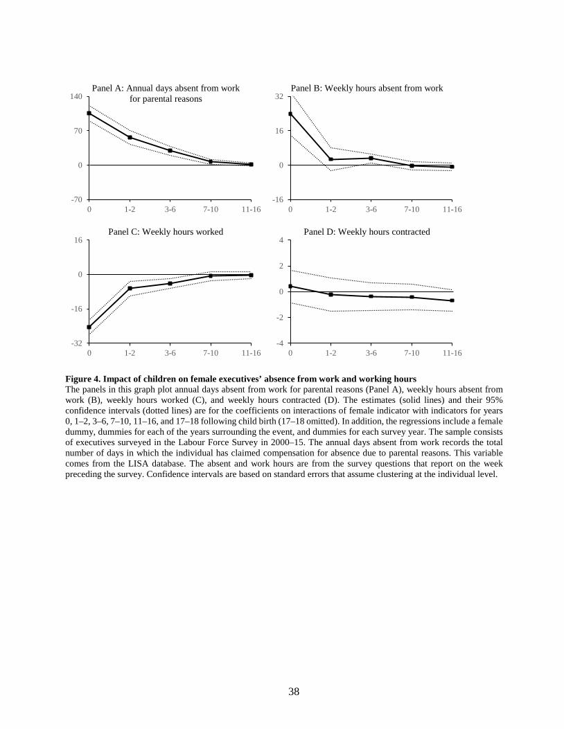
38

Figure 4. Impact of children on female executives’ absence from work and working hours The panels in this graph plot annual days absent from work for parental reasons (Panel A), weekly hours absent from work (B), weekly hours worked (C), and weekly hours contracted (D). The estimates (solid lines) and their 95% confidence intervals (dotted lines) are for the coefficients on interactions of female indicator with indicators for years 0, 1–2, 3–6, 7–10, 11–16, and 17–18 following child birth (17–18 omitted). In addition, the regressions include a female dummy, dummies for each of the years surrounding the event, and dummies for each survey year. The sample consists of executives surveyed in the Labour Force Survey in 2000–15. The annual days absent from work records the total number of days in which the individual has claimed compensation for absence due to parental reasons. This variable comes from the LISA database. The absent and work hours are from the survey questions that report on the week preceding the survey. Confidence intervals are based on standard errors that assume clustering at the individual level.

-70

0

70

140

0 1-2 3-6 7-10 11-16

Panel A: Annual days absent from work for parental reasons

-16

0

16

32

0 1-2 3-6 7-10 11-16

Panel B: Weekly hours absent from work

-32

-16

0

16

0 1-2 3-6 7-10 11-16

Panel C: Weekly hours worked

-4

-2

0

2

4

0 1-2 3-6 7-10 11-16

Panel D: Weekly hours contracted

39

Table 1 Gender gaps in top executive appointments and pay

The sample consists of executives of all Swedish limited-liability companies in 2011 with at least 10 employees and information on sales available. Panel A reports the gender gaps in the probability of attaining a top executive position. We define top executives in three different and in much extent overlapping ways. Large-firm CEOs hold the CEO position in firms with sales of at least SEK 500 million whereas large-firm top executives are the CEO and the four highest paid executives in these large firms. Highly paid executives have an annual labor income of at least SEK 1 million. The gender gap equals the female-male difference in the probability of attaining a top executive position and the robust t-statistic tests whether the gender gap differs from zero. Panel B reports mean and median pay for the three definitions of top executives and all executives. The log gender gap is the female-male difference in logged labor income and the robust t-statistic tests whether the gender gap differs from zero. Labor income includes all income taxed as labor income in a given year; base salaries, stock option grants, bonus payments, and benefits received from the employer qualify as taxable labor income. Tax authorities deem the taxable income to occur in the year when an employee or executive exercises her stock options or purchases her company’s shares at a price that is less than their fair value. The income is deflated to 2011 value and is expressed in million SEK.

Panel A: Probability of attaining a top executive position Large-firm CEOs Large-firm top executives Highly paid executives

Top execu-tives

Other execu-tives

Fraction top

execu-tives, %

Top

execu-tives

Other execu-tives

Fraction top

execu-tives, %

Top

execu-tives

Other execu-tives

Fraction top

execu-tives, %

All 300 24,062 1.23 1,479 22,883 6.07 3,160 21,202 12.97 Women 51 6,591 0.77 317 6,325 4.77 634 6,008 9.55 Men 249 17,471 1.41 1,162 16,558 6.56 2,526 15,194 14.26 Frac. women, % 17.00 27.39 21.43 27.64 20.06 28.34 Gender gap -0.64 -1.78 -4.71 t-value (-4.59) (-5.56) (-10.56)

Panel B: Mean pay in SEK millions Large-firm CEOs Large-firm top

executives Highly paid

executives All executives

Mean Median Mean Median Mean Median Mean Median All 2.08 1.72 1.34 1.09 1.55 1.29 0.69 0.58 Women 1.99 1.64 1.23 1.00 1.49 1.26 0.63 0.55 Men 2.10 1.78 1.37 1.11 1.56 1.30 0.72 0.59 Log gender gap, % -3.29 -9.26 -3.20 -11.59 t-value (-0.40) (-2.85) (-2.16) (-12.38)

40

Table 2 Gender differences in executive attributes

This table reports gender differences in the sample executives’ attributes. Panel A reports on the level of education and educational specialization. Panel B reports on career and networks. Top income education track takes the value of one if the combination of the level of education and educational specialization is among the top-5 specializations in 2011 in median total income and it has more than 100 graduates. Top executive education track takes the value of one if the combination of the level of education and educational specialization is among the top-5 specializations in 2011 in the number of large-firm top executives. Top executive high school takes the value of one if the high school is in the top-5 high schools in 2011 in terms of the fraction of graduates that become large-firm top executives and if it has more than 100 graduates. All the career variables except for unemployment are calculated using data from 1990 to 2011; the unemployment data is available from 1992. Unemployment is measured using information on the days the individual has collected unemployment benefits. Consulting or IB experience measures work experience from the following industries: Business and management consultancy activities (SNI2002, SNI1992=74140), Business and other management consultancy (SNI2007=70220), Security broking and fund management (SNI2002, SNI1992=67120), or Investment fund management activities (SNI2007=66301). Graduated in recession takes the value of one if the executive graduated in a year when Sweden experienced negative GDP growth (1977, 1991, 1992, or 1993). Panel C reports the means of indicators for having gained experience from different executive functions in 2004–09. Function is not observed for executives who did not hold a functional role during this period. Panel D reports on family background and risk tolerance. Birth order and Number of siblings have been calculated using data on all individuals of at least 16 years of age since 1990. Born in top-3 city takes the value of one if the individual has been born in Stockholm, Göteborg, or Malmö. Immigrant takes the value of one if the individual has been born outside of Sweden. Work in birth county indicates executives whose county of work is the same as their place of birth. Stock market participant uses data on direct stock holdings and indirect holdings via mutual funds. Panel E reports on parents’ socioeconomic status, and personal traits. Parents' socioeconomic status is measured using data from year 1990. Parent’s rank in age-gender income distribution refers to their labor income rank among all individuals of the same gender in a given cohort. Labor income includes all income taxed as labor income in a given year; base salaries, stock option grants, bonus payments, and benefits received from the employer qualify as taxable labor income. Tax authorities deem the taxable income to occur in the year when an employee or executive exercises her stock options or purchases her company’s shares at a price that is less than their fair value. Personal traits come from enlistment tests conducted on male conscripts around age 18. These data cover individuals born between 1951 and 1978. The traits are imputed using test scores of an executive’s randomly selected brother. Except for Imputed officer rank, a dummy for the reserve officer rank, a summary measure of aptitude and performance in the military, the variables are expressed as differences in standard deviations from the cohort mean. Imputed cognitive ability is based on four different subtests of inductive reasoning, verbal comprehension, spatial ability, and technical comprehension. The summary result of these tests is on a stanine scale. Imputed non-cognitive ability is assessed using psychological test results and semi-structured interviews. This test evaluates each conscript’s social maturity, intensity, psychological energy, and emotional stability and its summary result is on a stanine scale. Imputed physical fitness comes from a cycle ergometry test and Imputed muscular strength is a combination of knee extension, elbow flexion, and hand grip tests. Imputed body mass index is the ratio of weight in kilograms and squared height in meters. Imputed high school GPA is the grade point average in the final year of high school.

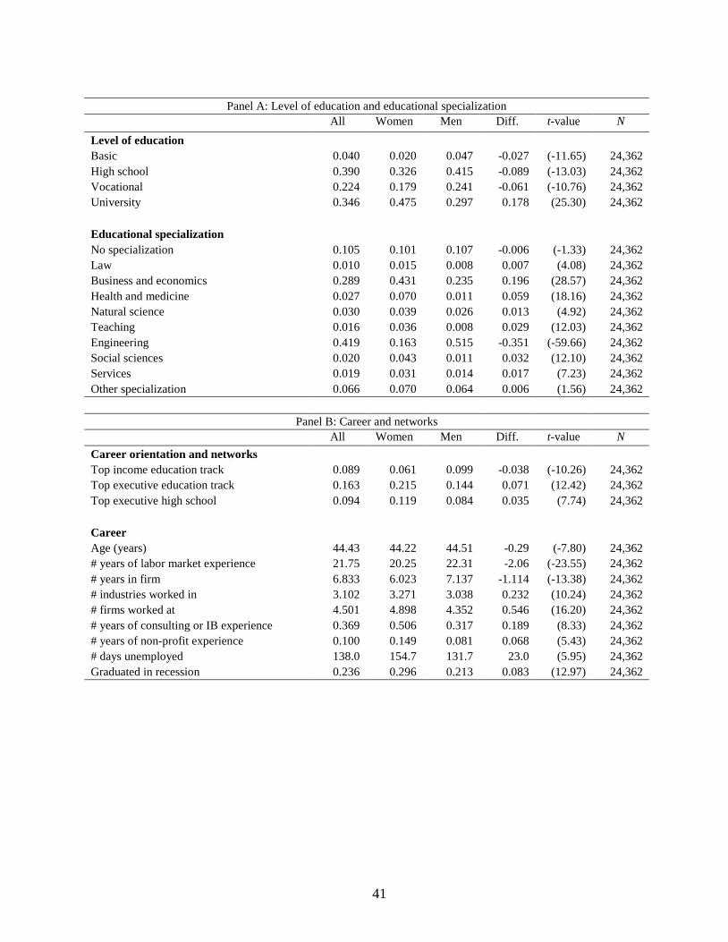
41

Panel A: Level of education and educational specialization

All Women Men Diff. t-value N Level of education Basic 0.040 0.020 0.047 -0.027 (-11.65) 24,362 High school 0.390 0.326 0.415 -0.089 (-13.03) 24,362 Vocational 0.224 0.179 0.241 -0.061 (-10.76) 24,362 University 0.346 0.475 0.297 0.178 (25.30) 24,362 Educational specialization No specialization 0.105 0.101 0.107 -0.006 (-1.33) 24,362 Law 0.010 0.015 0.008 0.007 (4.08) 24,362 Business and economics 0.289 0.431 0.235 0.196 (28.57) 24,362 Health and medicine 0.027 0.070 0.011 0.059 (18.16) 24,362 Natural science 0.030 0.039 0.026 0.013 (4.92) 24,362 Teaching 0.016 0.036 0.008 0.029 (12.03) 24,362 Engineering 0.419 0.163 0.515 -0.351 (-59.66) 24,362 Social sciences 0.020 0.043 0.011 0.032 (12.10) 24,362 Services 0.019 0.031 0.014 0.017 (7.23) 24,362 Other specialization 0.066 0.070 0.064 0.006 (1.56) 24,362

Panel B: Career and networks All Women Men Diff. t-value N

Career orientation and networks Top income education track 0.089 0.061 0.099 -0.038 (-10.26) 24,362 Top executive education track 0.163 0.215 0.144 0.071 (12.42) 24,362 Top executive high school 0.094 0.119 0.084 0.035 (7.74) 24,362 Career Age (years) 44.43 44.22 44.51 -0.29 (-7.80) 24,362 # years of labor market experience 21.75 20.25 22.31 -2.06 (-23.55) 24,362 # years in firm 6.833 6.023 7.137 -1.114 (-13.38) 24,362 # industries worked in 3.102 3.271 3.038 0.232 (10.24) 24,362 # firms worked at 4.501 4.898 4.352 0.546 (16.20) 24,362 # years of consulting or IB experience 0.369 0.506 0.317 0.189 (8.33) 24,362 # years of non-profit experience 0.100 0.149 0.081 0.068 (5.43) 24,362 # days unemployed 138.0 154.7 131.7 23.0 (5.95) 24,362 Graduated in recession 0.236 0.296 0.213 0.083 (12.97) 24,362

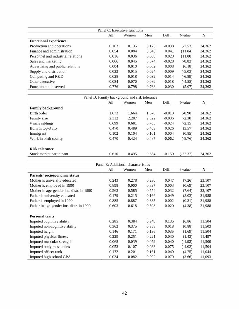
42

Panel C: Executive functions All Women Men Diff. t-value N

Functional experience Production and operations 0.163 0.135 0.173 -0.038 (-7.53) 24,362 Finance and administration 0.054 0.084 0.043 0.041 (11.04) 24,362 Personnel and industrial relations 0.016 0.036 0.008 0.028 (11.88) 24,362 Sales and marketing 0.066 0.045 0.074 -0.028 (-8.83) 24,362 Advertising and public relations 0.004 0.010 0.002 0.008 (6.18) 24,362 Supply and distribution 0.022 0.015 0.024 -0.009 (-5.03) 24,362 Computing and R&D 0.028 0.018 0.032 -0.014 (-6.89) 24,362 Other executive 0.084 0.070 0.089 -0.018 (-4.88) 24,362 Function not observed 0.776 0.798 0.768 0.030 (5.07) 24,362

Panel D: Family background and risk tolerance All Women Men Diff. t-value N

Family background Birth order 1.673 1.664 1.676 -0.013 (-0.98) 24,362 Family size 2.312 2.287 2.322 -0.036 (-2.38) 24,362 # male siblings 0.699 0.681 0.705 -0.024 (-2.15) 24,362 Born in top-3 city 0.470 0.489 0.463 0.026 (3.57) 24,362 Immigrant 0.102 0.104 0.101 0.004 (0.85) 24,362 Work in birth county 0.470 0.424 0.487 -0.062 (-8.76) 24,362 Risk tolerance Stock market participant 0.610 0.495 0.654 -0.159 (-22.37) 24,362

Panel E: Additional characteristics All Women Men Diff. t-value N

Parents' socioeconomic status Mother is university educated 0.243 0.278 0.230 0.047 (7.26) 23,107 Mother is employed in 1990 0.898 0.900 0.897 0.003 (0.69) 23,107 Mother in age-gender inc. distr. in 1990 0.562 0.585 0.554 0.032 (7.64) 23,107 Father is university educated 0.179 0.215 0.166 0.049 (8.03) 21,988 Father is employed in 1990 0.885 0.887 0.885 0.002 (0.31) 21,988 Father in age-gender inc. distr. in 1990 0.603 0.618 0.598 0.020 (4.38) 21,988 Personal traits Imputed cognitive ability 0.285 0.384 0.248 0.135 (6.86) 11,504 Imputed non-cognitive ability 0.362 0.375 0.358 0.018 (0.88) 11,503 Imputed height 0.146 0.171 0.136 0.035 (1.69) 11,504 Imputed physical fitness 0.229 0.251 0.221 0.030 (1.43) 11,497 Imputed muscular strength 0.068 0.039 0.079 -0.040 (-1.92) 11,500 Imputed body mass index -0.053 -0.107 -0.033 -0.075 (-4.02) 11,504 Imputed officer rank 0.172 0.201 0.161 0.040 (4.75) 11,044 Imputed high school GPA 0.024 0.082 0.002 0.079 (3.66) 11,093

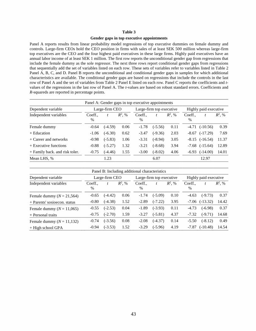
43

Table 3 Gender gaps in top executive appointments

Panel A reports results from linear probability model regressions of top executive dummies on female dummy and controls. Large-firm CEOs hold the CEO position in firms with sales of at least SEK 500 million whereas large-firm top executives are the CEO and the four highest paid executives in these large firms. Highly paid executives have an annual labor income of at least SEK 1 million. The first row reports the unconditional gender gap from regressions that include the female dummy as the sole regressor. The next three rows report conditional gender gaps from regressions that sequentially add the set of variables listed on each row. These sets of variables refer to variables listed in Table 2 Panel A, B, C, and D. Panel B reports the unconditional and conditional gender gaps in samples for which additional characteristics are available. The conditional gender gaps are based on regressions that include the controls in the last row of Panel A and the set of variables from Table 2 Panel E listed on each row. Panel C reports the coefficients and t-values of the regressions in the last row of Panel A. The t-values are based on robust standard errors. Coefficients and R-squareds are reported in percentage points.

Panel A: Gender gaps in top executive appointments Dependent variable Large-firm CEO Large-firm top executive Highly paid executive Independent variables

Coeff.,

% t R2, %

Coeff.,

% t R2, %

Coeff.,

% t R2, %

Female dummy -0.64 (-4.59) 0.06 -1.78 (-5.56) 0.11 -4.71 (-10.56) 0.39 + Education -1.06 (-6.30) 0.62 -3.47 (-9.36) 2.03 -8.67 (-17.29) 7.69 + Career and networks -0.98 (-5.83) 1.06 -3.31 (-8.94) 3.05 -8.15 (-16.54) 11.37 + Executive functions -0.88 (-5.27) 1.32 -3.21 (-8.68) 3.94 -7.68 (-15.64) 12.89 + Family back. and risk toler. -0.75 (-4.46) 1.55 -3.00 (-8.02) 4.06 -6.93 (-14.00) 14.01 Mean LHS, % 1.23 6.07 12.97

Panel B: Including additional characteristics Dependent variable Large-firm CEO Large-firm top executive Highly paid executive Independent variables

Coeff.,

% t R2, %

Coeff.,

% t R2, %

Coeff.,

% t R2, %

Female dummy (N = 21,564) -0.65 (-4.42) 0.06 -1.74 (-5.09) 0.10 -4.63 (-9.73) 0.37

+ Parents' sosioecon. status -0.80 (-4.38) 1.52 -2.89 (-7.22) 3.95 -7.06 (-13.32) 14.42

Female dummy (N = 11,065) -0.55 (-2.53) 0.04 -1.89 (-3.93) 0.11 -4.73 (-6.98) 0.37

+ Personal traits -0.75 (-2.70) 1.59 -3.27 (-5.81) 4.37 -7.32 (-9.71) 14.68

Female dummy (N = 11,132) -0.74 (-3.56) 0.08 -2.08 (-4.37) 0.14 -5.50 (-8.12) 0.49

+ High school GPA -0.94 (-3.53) 1.52 -3.29 (-5.96) 4.19 -7.87 (-10.48) 14.54

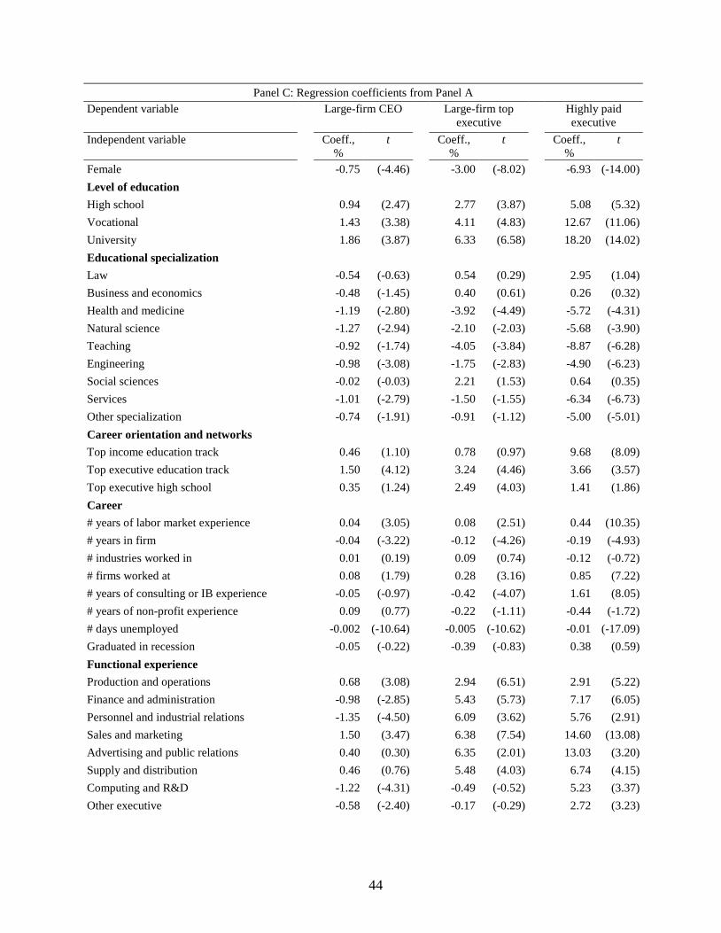
44

Panel C: Regression coefficients from Panel A Dependent variable

Large-firm CEO

Large-firm top

executive

Highly paid executive

Independent variable

Coeff., %

t

Coeff., %

t

Coeff., %

t

Female -0.75 (-4.46) -3.00 (-8.02) -6.93 (-14.00) Level of education High school 0.94 (2.47) 2.77 (3.87) 5.08 (5.32) Vocational 1.43 (3.38) 4.11 (4.83) 12.67 (11.06) University 1.86 (3.87) 6.33 (6.58) 18.20 (14.02) Educational specialization Law -0.54 (-0.63) 0.54 (0.29) 2.95 (1.04) Business and economics -0.48 (-1.45) 0.40 (0.61) 0.26 (0.32) Health and medicine -1.19 (-2.80) -3.92 (-4.49) -5.72 (-4.31) Natural science -1.27 (-2.94) -2.10 (-2.03) -5.68 (-3.90) Teaching -0.92 (-1.74) -4.05 (-3.84) -8.87 (-6.28) Engineering -0.98 (-3.08) -1.75 (-2.83) -4.90 (-6.23) Social sciences -0.02 (-0.03) 2.21 (1.53) 0.64 (0.35) Services -1.01 (-2.79) -1.50 (-1.55) -6.34 (-6.73) Other specialization -0.74 (-1.91) -0.91 (-1.12) -5.00 (-5.01) Career orientation and networks Top income education track 0.46 (1.10) 0.78 (0.97) 9.68 (8.09) Top executive education track 1.50 (4.12) 3.24 (4.46) 3.66 (3.57) Top executive high school 0.35 (1.24) 2.49 (4.03) 1.41 (1.86) Career # years of labor market experience 0.04 (3.05) 0.08 (2.51) 0.44 (10.35) # years in firm -0.04 (-3.22) -0.12 (-4.26) -0.19 (-4.93) # industries worked in 0.01 (0.19) 0.09 (0.74) -0.12 (-0.72) # firms worked at 0.08 (1.79) 0.28 (3.16) 0.85 (7.22) # years of consulting or IB experience -0.05 (-0.97) -0.42 (-4.07) 1.61 (8.05) # years of non-profit experience 0.09 (0.77) -0.22 (-1.11) -0.44 (-1.72) # days unemployed -0.002 (-10.64) -0.005 (-10.62) -0.01 (-17.09) Graduated in recession -0.05 (-0.22) -0.39 (-0.83) 0.38 (0.59) Functional experience Production and operations 0.68 (3.08) 2.94 (6.51) 2.91 (5.22) Finance and administration -0.98 (-2.85) 5.43 (5.73) 7.17 (6.05) Personnel and industrial relations -1.35 (-4.50) 6.09 (3.62) 5.76 (2.91) Sales and marketing 1.50 (3.47) 6.38 (7.54) 14.60 (13.08) Advertising and public relations 0.40 (0.30) 6.35 (2.01) 13.03 (3.20) Supply and distribution 0.46 (0.76) 5.48 (4.03) 6.74 (4.15) Computing and R&D -1.22 (-4.31) -0.49 (-0.52) 5.23 (3.37) Other executive -0.58 (-2.40) -0.17 (-0.29) 2.72 (3.23)

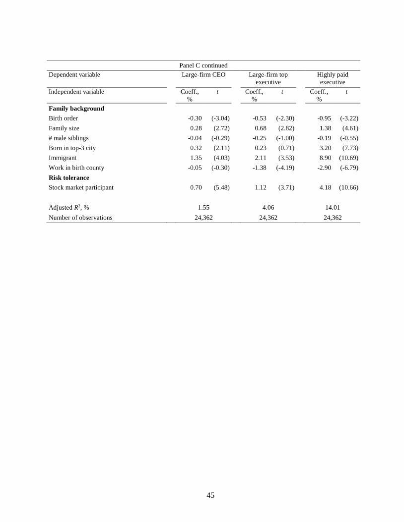
45

Panel C continued Dependent variable

Large-firm CEO

Large-firm top

executive

Highly paid executive

Independent variable

Coeff., %

t

Coeff., %

t

Coeff., %

t

Family background Birth order -0.30 (-3.04) -0.53 (-2.30) -0.95 (-3.22) Family size 0.28 (2.72) 0.68 (2.82) 1.38 (4.61) # male siblings -0.04 (-0.29) -0.25 (-1.00) -0.19 (-0.55) Born in top-3 city 0.32 (2.11) 0.23 (0.71) 3.20 (7.73) Immigrant 1.35 (4.03) 2.11 (3.53) 8.90 (10.69) Work in birth county -0.05 (-0.30) -1.38 (-4.19) -2.90 (-6.79) Risk tolerance Stock market participant 0.70 (5.48) 1.12 (3.71) 4.18 (10.66) Adjusted R2, % 1.55 4.06 14.01 Number of observations 24,362 24,362 24,362

46

Table 4 Gender differences in family-related characteristics

This table reports gender differences in the sample executives’ attributes that relate to their family. Panel A reports the marital status, number of children, and number of children who live in the executive’s household in 2011. The married category includes both legal marriages and registered partnerships. The number of children has been calculated using data on all individuals of at least 16 years of age since 1990.

All execu-tives

Women Men N Women less men All

execu-tives

Large-firm

CEOs

Large-firm top execu-tives

Highly paid

execu-tive

Married 0.700 0.658 0.716 24,362 -0.058 -0.185 -0.093 -0.099 (-8.58) (-2.70) (-3.38) (-5.20) Divorced 0.075 0.104 0.063 24,362 0.041 0.085 0.083 0.042 (9.80) (1.69) (4.11) (3.24) Single 0.225 0.238 0.221 24,362 0.017 0.100 0.011 0.057 (2.78) (1.78) (0.49) (3.58) Has children 0.915 0.894 0.923 24,362 -0.029 0.000 -0.041 -0.065 (-6.74) (0.02) (-2.47) (-5.10) # children 1.919 1.699 2.002 24,362 -0.303 -0.279 -0.376 -0.409 (-23.87) (-2.69) (-7.44) (-10.86) # children at home 1.749 1.699 1.767 24,362 -0.068 -0.026 -0.144 -0.190 (-5.27) (-0.24) (-2.78) (-4.95) First child born at age 29.62 29.48 29.68 22,287 -0.197 0.415 -0.015 -0.033 (-4.09) (1.19) (-0.08) (-0.26)

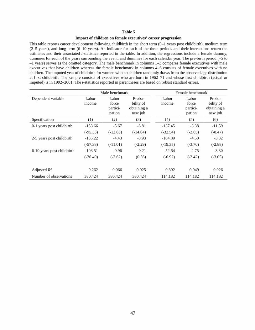
47

Table 5 Impact of children on female executives’ career progression

This table reports career development following childbirth in the short term (0–1 years post childbirth), medium term (2–5 years), and long term (6–10 years). An indicator for each of the three periods and their interactions return the estimates and their associated t-statistics reported in the table. In addition, the regressions include a female dummy, dummies for each of the years surrounding the event, and dummies for each calendar year. The pre-birth period (–5 to –1 years) serves as the omitted category. The male benchmark in columns 1–3 compares female executives with male executives that have children whereas the female benchmark in columns 4–6 consists of female executives with no children. The imputed year of childbirth for women with no children randomly draws from the observed age distribution at first childbirth. The sample consists of executives who are born in 1962–71 and whose first childbirth (actual or imputed) is in 1992–2001. The t-statistics reported in parentheses are based on robust standard errors.

Male benchmark Female benchmark Dependent variable Labor

income Labor force

partici-pation

Proba-bility of

obtaining a new job

Labor

income Labor force

partici-pation

Proba-bility of

obtaining a new job

Specification (1) (2) (3) (4) (5) (6) 0-1 years post childbirth -153.66 -5.67 -6.81 -137.45 -3.38 -11.59 (-95.33) (-12.83) (-14.04) (-32.54) (-2.65) (-8.47) 2-5 years post childbirth -135.22 -4.43 -0.93 -104.89 -4.50 -3.32 (-57.38) (-11.01) (-2.29) (-19.35) (-3.70) (-2.88) 6-10 years post childbirth -103.51 -0.96 0.21 -52.64 -2.75 -3.30 (-26.49) (-2.62) (0.56) (-6.92) (-2.42) (-3.05) Adjusted R2 0.262 0.066 0.025 0.302 0.049 0.026 Number of observations 380,424 380,424 380,424 114,182 114,182 114,182

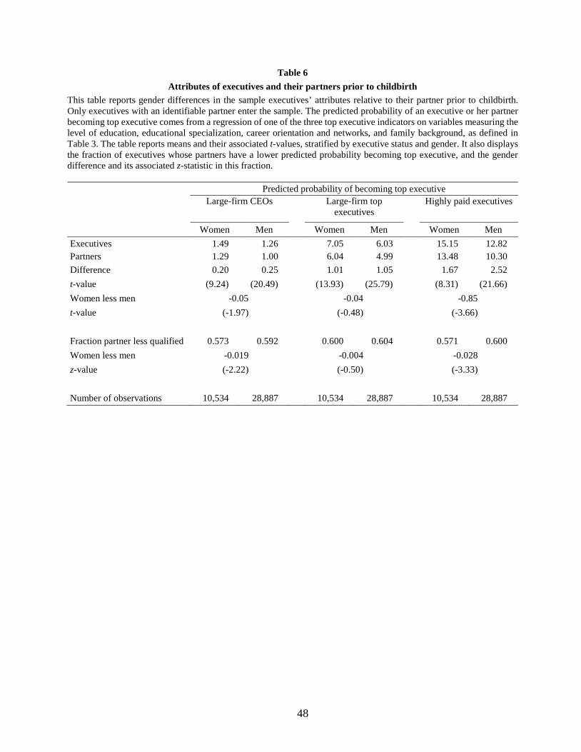
48

Table 6 Attributes of executives and their partners prior to childbirth

This table reports gender differences in the sample executives’ attributes relative to their partner prior to childbirth. Only executives with an identifiable partner enter the sample. The predicted probability of an executive or her partner becoming top executive comes from a regression of one of the three top executive indicators on variables measuring the level of education, educational specialization, career orientation and networks, and family background, as defined in Table 3. The table reports means and their associated t-values, stratified by executive status and gender. It also displays the fraction of executives whose partners have a lower predicted probability becoming top executive, and the gender difference and its associated z-statistic in this fraction. Predicted probability of becoming top executive

Large-firm CEOs

Large-firm top

executives

Highly paid executives

Women Men Women Men Women Men Executives 1.49 1.26 7.05 6.03 15.15 12.82 Partners 1.29 1.00 6.04 4.99 13.48 10.30 Difference 0.20 0.25 1.01 1.05 1.67 2.52 t-value (9.24) (20.49) (13.93) (25.79) (8.31) (21.66) Women less men -0.05 -0.04 -0.85 t-value (-1.97) (-0.48) (-3.66) Fraction partner less qualified 0.573 0.592 0.600 0.604 0.571 0.600 Women less men -0.019 -0.004 -0.028 z-value (-2.22) (-0.50) (-3.33) Number of observations 10,534 28,887 10,534 28,887 10,534 28,887

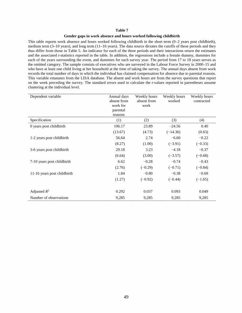
49

Table 7 Gender gaps in work absence and hours worked following childbirth

This table reports work absence and hours worked following childbirth in the short term (0–2 years post childbirth), medium term (3–10 years), and long term (11–16 years). The data source dictates the cutoffs of these periods and they thus differ from those in Table 5. An indicator for each of the three periods and their interactions return the estimates and the associated t-statistics reported in the table. In addition, the regressions include a female dummy, dummies for each of the years surrounding the event, and dummies for each survey year. The period from 17 to 18 years serves as the omitted category. The sample consists of executives who are surveyed in the Labour Force Survey in 2000–15 and who have at least one child living at her household at the time of taking the survey. The annual days absent from work records the total number of days in which the individual has claimed compensation for absence due to parental reasons. This variable emanates from the LISA database. The absent and work hours are from the survey questions that report on the week preceding the survey. The standard errors used to calculate the t-values reported in parentheses assume clustering at the individual level.

Dependent variable Annual days absent from

work for parental reasons

Weekly hours absent from

work

Weekly hours worked

Weekly hours contracted

Specification (1) (2) (3) (4) 0 years post childbirth 106.17 23.89 −24.56 0.40 (13.67) (4.73) (−14.36) (0.63) 1-2 years post childbirth 56.64 2.74 −6.60 −0.22 (8.27) (1.00) (−3.91) (−0.33) 3-6 years post childbirth 29.18 3.23 −4.18 −0.37 (6.64) (3.00) (−3.57) (−0.68) 7-10 years post childbirth 6.62 −0.28 −0.74 −0.43 (2.76) (−0.29) (−0.71) (−0.84) 11-16 years post childbirth 1.84 −0.80 −0.38 −0.69 (1.27) (−0.92) (−0.44) (−1.65) Adjusted R2 0.292 0.037 0.093 0.049 Number of observations 9,285 9,285 9,285 9,285

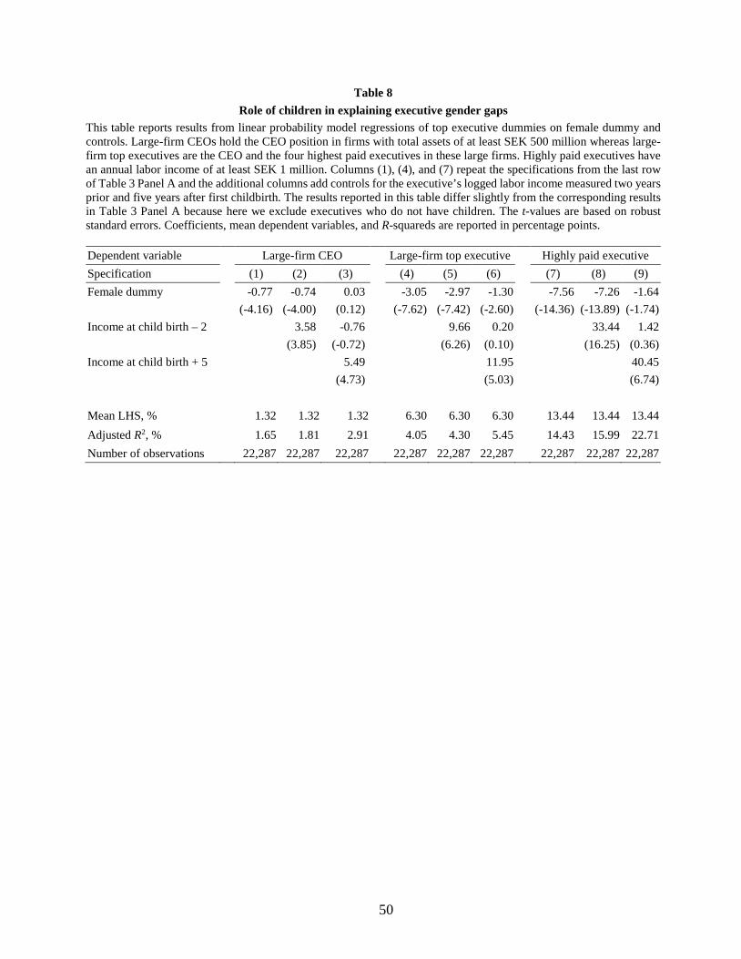
50

Table 8 Role of children in explaining executive gender gaps

This table reports results from linear probability model regressions of top executive dummies on female dummy and controls. Large-firm CEOs hold the CEO position in firms with total assets of at least SEK 500 million whereas large-firm top executives are the CEO and the four highest paid executives in these large firms. Highly paid executives have an annual labor income of at least SEK 1 million. Columns (1), (4), and (7) repeat the specifications from the last row of Table 3 Panel A and the additional columns add controls for the executive’s logged labor income measured two years prior and five years after first childbirth. The results reported in this table differ slightly from the corresponding results in Table 3 Panel A because here we exclude executives who do not have children. The t-values are based on robust standard errors. Coefficients, mean dependent variables, and R-squareds are reported in percentage points. Dependent variable Large-firm CEO Large-firm top executive Highly paid executive Specification (1) (2) (3) (4) (5) (6) (7) (8) (9) Female dummy -0.77 -0.74 0.03 -3.05 -2.97 -1.30 -7.56 -7.26 -1.64 (-4.16) (-4.00) (0.12) (-7.62) (-7.42) (-2.60) (-14.36) (-13.89) (-1.74) Income at child birth – 2 3.58 -0.76 9.66 0.20 33.44 1.42 (3.85) (-0.72) (6.26) (0.10) (16.25) (0.36) Income at child birth + 5 5.49 11.95 40.45 (4.73) (5.03) (6.74) Mean LHS, % 1.32 1.32 1.32 6.30 6.30 6.30 13.44 13.44 13.44 Adjusted R2, % 1.65 1.81 2.91 4.05 4.30 5.45 14.43 15.99 22.71 Number of observations 22,287 22,287 22,287 22,287 22,287 22,287 22,287 22,287 22,287

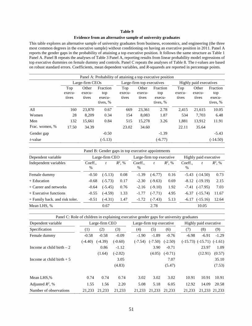
51

Table 9 Evidence from an alternative sample of university graduates

This table explores an alternative sample of university graduates from business, economics, and engineering (the three most common degrees in the executive sample) without conditioning on having an executive position in 2011. Panel A reports the gender gaps in the probability of attaining a top executive position. It follows the same structure as Table 1 Panel A. Panel B repeats the analyses of Table 3 Panel A, reporting results from linear probability model regressions of top executive dummies on female dummy and controls. Panel C repeats the analyses of Table 8. The t-values are based on robust standard errors. Coefficients, mean dependent variables, and R-squareds are reported in percentage points.

Panel A: Probability of attaining a top executive position Large-firm CEOs Large-firm top executives Highly paid executives

Top execu-tives

Other execu-tives

Fraction top

execu-tives, %

Top

execu-tives

Other execu-tives

Fraction top

execu-tives, %

Top

execu-tives

Other execu-tives

Fraction top

execu-tives, %

All 160 23,870 0.67 669 23,361 2.78 2,415 21,615 10.05 Women 28 8,209 0.34 154 8,083 1.87 534 7,703 6.48 Men 132 15,661 0.84 515 15,278 3.26 1,881 13,912 11.91 Frac. women, % 17.50 34.39 23.02 34.60 22.11 35.64 Gender gap -0.50 -1.39 -5.43 t-value (-5.13) (-6.77) (-14.50)

Panel B: Gender gaps in top executive appointments Dependent variable Large-firm CEO Large-firm top executive Highly paid executive Independent variables

Coeff.,

% t R2, %

Coeff.,

% t R2, %

Coeff.,

% t R2, %

Female dummy -0.50 (-5.13) 0.08 -1.39 (-6.77) 0.16 -5.43 (-14.50) 0.73 + Education -0.68 (-5.73) 0.17 -2.30 (-9.63) 0.69 -8.12 (-19.19) 2.15 + Career and networks -0.64 (-5.45) 0.76 -2.16 (-9.10) 1.92 -7.41 (-17.95) 7.03 + Executive functions -0.55 (-4.59) 1.33 -1.77 (-7.71) 4.95 -6.37 (-15.74) 11.67 + Family back. and risk toler. -0.51 (-4.31) 1.47 -1.72 (-7.43) 5.13 -6.17 (-15.16) 12.64 Mean LHS, % 0.67 2.78 10.05

Panel C: Role of children in explaining executive gender gaps for university graduates Dependent variable Large-firm CEO Large-firm top executive Highly paid executive Specification (1) (2) (3) (4) (5) (6) (7) (8) (9) Female dummy -0.58 -0.58 -0.09 -1.90 -1.89 -0.76 -6.98 -6.91 -1.29 (-4.40) (-4.39) (-0.60) (-7.54) (-7.50) (-2.50) (-15.73) (-15.71) (-1.61) Income at child birth – 2 0.86 -1.12 3.90 -0.71 23.97 1.09 (1.64) (-2.02) (4.05) (-0.71) (12.91) (0.57) Income at child birth + 5 3.05 7.07 35.10 (4.83) (5.47) (7.53) Mean LHS,% 0.74 0.74 0.74 3.02 3.02 3.02 10.91 10.91 10.91 Adjusted R2, % 1.55 1.56 2.20 5.08 5.18 6.05 12.92 14.09 20.58 Number of observations 21,233 21,233 21,233 21,233 21,233 21,233 21,233 21,233 21,233

Internet Appendix for

What Prevents Female Executives from Reaching the Top?

Matti Keloharju

Aalto University School of Business, CEPR, and IFN

Samuli Knüpfer

BI Norwegian Business School, CEPR, and IFN

Joacim Tåg

Research Institute of Industrial Economics (IFN)

December 15, 2017

1

Figure IA1. Likelihood to live in birth county by gender and age This figure displays the fraction of female and male executives that live in their birth county as a function of their age. The sample consists of executives who are born in 1962–71.

0.0

0.2

0.4

0.6

0.8

1.0

19 21 23 25 27 29 31 33 35 37 39 41 43 45 47 49

Prob

abili

ty o

f liv

ing

in b

irth

coun

ty

Age

Male executivesFemale executives

2

Figure IA2. Impact of children on female executives that have one child The panels in this graph plot annual labor income relative to the birth year of the executive’s first child. The estimates (solid lines) and their 95% confidence intervals (dotted lines) are for the coefficients on interactions of female indicator with indicators for the 15 years surrounding the event of childbirth (–5 omitted). The male benchmark compares female executives with male executives that have children whereas the female benchmark consists of female executives with no children. The imputed year of childbirth for women with no children randomly draws from the observed age distribution at first childbirth. The sample consists of executives who are born in 1962–1971 and whose first childbirth (actual or imputed) is in 1992–2001.

-200

-150

-100

-50

0

50

100

-4 -3 -2 -1 0 1 2 3 4 5 6 7 8 9 10

Panel A: Labor income (SEK thousands), male benchmark

-200

-150

-100

-50

0

50

100

-4 -3 -2 -1 0 1 2 3 4 5 6 7 8 9 10

Panel B: Labor income (SEK thousands), female benchmark

3

Figure IA3. Impact of children in sample of university graduates This figure repeats the analyses in Figure 2 for university graduates from business, economics, or engineering who are born in 1962–71 and whose first childbirth is in 1992–2001. Confidence intervals are based on standard errors that assume clustering at the individual level.

-250

-200

-150

-100

-50

0

50

100

-4 -3 -2 -1 0 1 2 3 4 5 6 7 8 9 10

Panel A: Labor income (SEK thousands), male benchmark

-250

-200

-150

-100

-50

0

50

100

-4 -3 -2 -1 0 1 2 3 4 5 6 7 8 9 10

Panel B: Labor income (SEK thousands), female benchmark

-15

-10

-5

0

5

10

15

-4 -3 -2 -1 0 1 2 3 4 5 6 7 8 9 10

Panel C: Labor force participation (%), male benchmark

-15

-10

-5

0

5

10

15

-4 -3 -2 -1 0 1 2 3 4 5 6 7 8 9 10

Panel D: Labor force participation (%), female benchmark

-25-20-15-10-505

1015

-4 -3 -2 -1 0 1 2 3 4 5 6 7 8 9 10

Panel E: Probability of attaining new job (%), male benchmark

-25-20-15-10-505

1015

-4 -3 -2 -1 0 1 2 3 4 5 6 7 8 9 10

Panel F: Probability of attaining new job (%), female benchmark

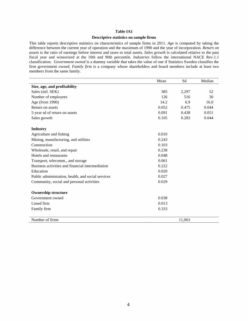
4

Table IA1 Descriptive statistics on sample firms

This table reports descriptive statistics on characteristics of sample firms in 2011. Age is computed by taking the difference between the current year of operation and the maximum of 1990 and the year of incorporation. Return on assets is the ratio of earnings before interest and taxes to total assets. Sales growth is calculated relative to the past fiscal year and winsorized at the 10th and 90th percentile. Industries follow the international NACE Rev.1.1 classification. Government owned is a dummy variable that takes the value of one if Statistics Sweden classifies the firm government owned. Family firm is a company whose shareholders and board members include at least two members from the same family.

Mean Sd Median Size, age, and profitability Sales (mil. SEK) 385 2,297 52 Number of employees 126 516 30 Age (from 1990) 14.2 6.9 16.0 Return on assets 0.052 0.475 0.044 5-year sd of return on assets 0.091 0.438 0.051 Sales growth 0.105 0.283 0.044 Industry Agriculture and fishing 0.010 Mining, manufacturing, and utilities 0.243 Construction 0.103 Wholesale, retail, and repair 0.238 Hotels and restaurants 0.048 Transport, telecomm., and storage 0.061 Business activities and financial intermediation 0.222 Education 0.020 Public administration, health, and social services 0.027 Community, social and personal activities 0.029 Ownership structure Government owned 0.038 Listed firm 0.013 Family firm 0.333 Number of firms 11,063

5

Table IA2 Parents’ socioeconomic status as a function of trait imputation

This table reports socioeconomic status of an executive’s parents as a function of whether the executive’s traits are imputable from brother’s test scores. Parents' socioeconomic status is measured using data from year 1990. Parent’s rank in income distribution refers to their labor income rank among all individuals of the same gender in a given cohort. The four rightmost rows report the gender differences in parents’ socioeconomic status for imputed and non-imputed executives. The t-statistics are for the double difference by imputation status and gender.

Imputed Not imputed Impu-

ted Not

impu-ted

Diffe-rence

t-value

Wo-men

Men N Wo-men

Men N Wo-men less men

Wo-men less men

Mother University educated 0.902 0.901 11,230 0.898 0.893 11,877 0.001 0.005 -0.003 (-0.38) Employed 0.584 0.551 11,230 0.587 0.556 11,877 0.033 0.031 0.001 (0.15) Rank in income distr. 0.300 0.245 11,230 0.257 0.216 11,877 0.055 0.040 0.014 (1.11)

Father University educated 0.895 0.889 10,904 0.878 0.881 11,084 0.006 -0.003 0.009 (0.88) Employed 0.625 0.602 10,904 0.610 0.594 11,084 0.023 0.017 0.006 (0.64) Rank in income distr. 0.240 0.182 10,904 0.190 0.151 11,084 0.059 0.039 0.020 (1.65)

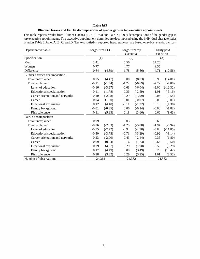
6

Table IA3 Blinder-Oaxaca and Fairlie decompositions of gender gaps in top executive appointments

This table reports results from Blinder-Oaxaca (1973, 1973) and Fairlie (1999) decompositions of the gender gap in top executive appointments. Top executive appointment dummies are decomposed using the individual characteristics listed in Table 2 Panel A, B, C, and D. The test statistics, reported in parentheses, are based on robust standard errors. Dependent variable

Large-firm CEO

Large-firm top

executive

Highly paid executive

Specification (1) (2) (3) Men 1.41 6.56 14.26 Women 0.77 4.77 9.55 Difference 0.64 (4.59) 1.78 (5.56) 4.71 (10.56) Blinder-Oaxaca decomposition

Total unexplained 0.75 (4.47) 3.00 (8.03) 6.93 (14.01) Total explained -0.11 (-1.54) -1.22 (-6.69) -2.22 (-7.80)

Level of education -0.16 (-3.27) -0.63 (-6.04) -2.00 (-12.32) Educational specialization -0.11 (-1.78) -0.36 (-2.59) -1.01 (-5.16) Career orientation and networks -0.10 (-2.98) -0.29 (-3.99) 0.06 (0.54) Career 0.04 (1.00) -0.01 (-0.07) 0.00 (0.01) Functional experience 0.12 (4.18) -0.11 (-1.32) 0.15 (1.38) Family background -0.01 (-0.95) 0.00 (-0.14) -0.08 (-1.82) Risk tolerance 0.11 (5.33) 0.18 (3.66) 0.66 (9.63)

Fairlie decomposition Total unexplained 0.99 3.03 6.65 Total explained -0.36 (-2.83) -1.25 (-5.88) -1.94 (-6.94)

Level of education -0.55 (-2.72) -0.94 (-4.38) -3.83 (-11.85) Educational specialization -0.50 (-3.75) -0.71 (-3.29) -0.92 (-3.14) Career orientation and networks -0.23 (-2.00) -0.43 (-2.44) 0.35 (1.80) Career 0.09 (0.94) 0.16 (1.23) 0.64 (3.50) Functional experience 0.39 (4.97) 0.29 (1.98) 0.55 (3.29) Family background 0.17 (4.49) 0.09 (3.49) 0.25 (10.42) Risk tolerance 0.28 (3.82) 0.29 (3.25) 1.01 (8.52)

Number of observations 24,362 24,362 24,362

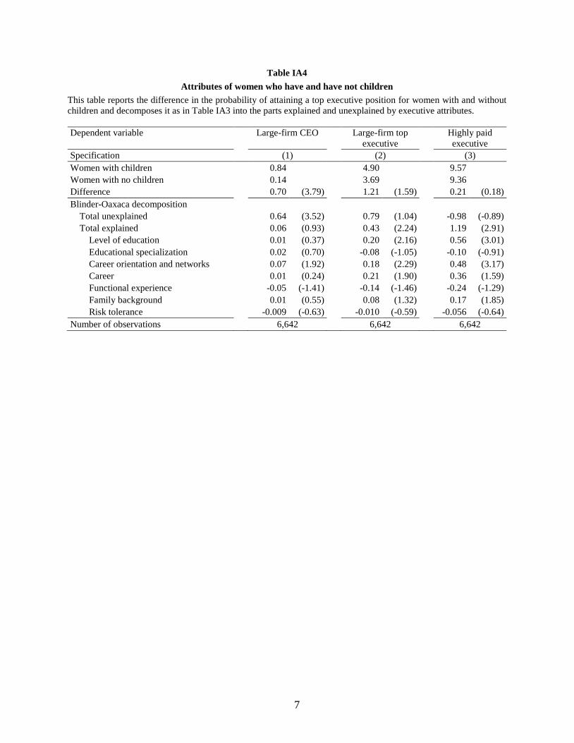
7

Table IA4 Attributes of women who have and have not children

This table reports the difference in the probability of attaining a top executive position for women with and without children and decomposes it as in Table IA3 into the parts explained and unexplained by executive attributes. Dependent variable

Large-firm CEO

Large-firm top

executive

Highly paid executive

Specification (1) (2) (3) Women with children 0.84 4.90 9.57 Women with no children 0.14 3.69 9.36 Difference 0.70 (3.79) 1.21 (1.59) 0.21 (0.18) Blinder-Oaxaca decomposition

Total unexplained 0.64 (3.52) 0.79 (1.04) -0.98 (-0.89) Total explained 0.06 (0.93) 0.43 (2.24) 1.19 (2.91)

Level of education 0.01 (0.37) 0.20 (2.16) 0.56 (3.01) Educational specialization 0.02 (0.70) -0.08 (-1.05) -0.10 (-0.91) Career orientation and networks 0.07 (1.92) 0.18 (2.29) 0.48 (3.17) Career 0.01 (0.24) 0.21 (1.90) 0.36 (1.59) Functional experience -0.05 (-1.41) -0.14 (-1.46) -0.24 (-1.29) Family background 0.01 (0.55) 0.08 (1.32) 0.17 (1.85) Risk tolerance -0.009 (-0.63) -0.010 (-0.59) -0.056 (-0.64)

Number of observations 6,642 6,642 6,642

8

Table IA5 Comparison of the executives in the main sample and in the Labour Force Survey sample

This table compares selected executive characteristics in the core sample and in the Labour Force Survey sample. It reports the means of each characteristic, their difference, and the difference’s robust t-statistic. The table covers annual waves of the survey in 2000–15.

Core sample

Labour Force

Survey

Diff. t-value N Core

sample

N Labour Force

Survey

Level of education Basic 0.040 0.053 -0.013 (-4.91) 24,362 9,275 High school 0.390 0.374 0.016 (2.74) 24,362 9,275 Vocational 0.224 0.233 -0.009 (-1.67) 24,362 9,275 University 0.346 0.341 0.005 (0.92) 24,362 9,275 Other characteristics Labor income (SEK millions) 0.694 0.607 0.087 (16.14) 24,362 9,285 Age (years) 44.43 42.31 2.12 (29.44) 24,362 9,285 Married 0.700 0.678 0.022 (3.91) 24,362 9,284

9

Table IA6 Robustness checks on impact of children on career progression

This table explores alternative definitions of top executive positions and an alternative sample. Panel A replicates the results of Table 8 by doubling the total assets cutoff to SEK 1 billion and the pay cutoff to SEK 2 million. Panel B uses a sample of executives who are 50–59 years old in 2011. Income measured two years prior to child birth drops out of these regressions as its measurement is not possible prior to1990. The t-values are based on robust standard errors. Coefficients, mean dependent variables, and R-squareds are reported in percentage points.

Panel A: Doubling firm-size and pay cutoffs Dependent variable Large-firm CEO Large-firm top executive Highly paid executive Specification (1) (2) (3) (4) (5) (6) (7) (8) (9) Female dummy -0.30 -0.28 0.15 -1.63 -1.56 -0.34 -1.81 -1.70 0.87 (-2.33) (-2.17) (0.98) (-5.40) (-5.17) (-0.92) (-7.77) (-7.36) (2.69) Income at child birth – 2 2.42 0.01 7.85 0.93 12.02 -2.58 (3.22) (0.02) (6.29) (0.61) (8.04) (-1.53) Income at child birth + 5 3.04 8.74 18.45 (4.29) (4.93) (9.41) Mean LHS, % 0.62 0.62 0.62 3.37 3.37 3.37 2.06 2.06 2.06 Adjusted R2, % 0.86 1.01 1.73 2.75 3.05 4.17 3.69 4.86 12.94 Number of observations 22,287 22,287 22,287 22,287 22,287 22,287 22,287 22,287 22,287

Panel B: Sample of executives aged 50–59 years Dependent variable

Large-firm CEO

Large-firm top executive

Highly paid executive

Specification (1) (2) (3) (4) (5) (6) Female dummy -1.07 -0.46 -3.39 -1.99 -7.80 -2.85 (-3.15) (-1.33) (-4.44) (-2.57) (-7.00) (-2.60) Income at child birth + 5 5.54 12.74 44.89 (5.75) (8.62) (19.22) Mean LHS, % 1.58 1.58 7.43 7.43 17.72 17.72 Adjusted R2, % 1.50 2.33 4.47 5.47 16.23 22.14 Number of observations 14,810 14,810 14,810 14,810 14,810 14,810