What We Will Cover in This Section

1

Statistics, an Overview 2

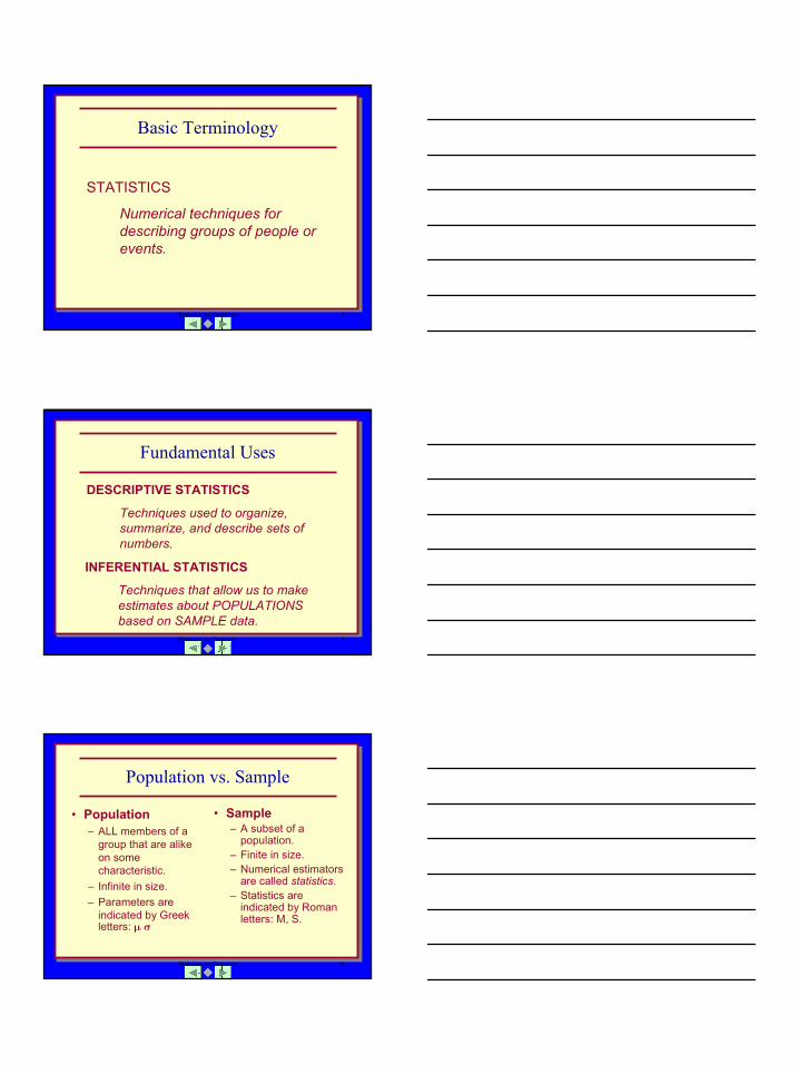
What We Will Cover in This Section

• What statistics are.• Descriptive Statistics

– Frequency distributions

– Graphs– Mean– Standard deviation

• Inferential Statistics– Z-scores

• Hypothesis Testing

Basic Terms and Concepts

2


Basic Terminology

STATISTICS

Numerical techniques for describing groups of people or events.


Fundamental Uses

DESCRIPTIVE STATISTICS

Techniques used to organize, summarize, and describe sets of numbers.

INFERENTIAL STATISTICS

Techniques that allow us to make estimates about POPULATIONS based on SAMPLE data.


Population vs. Sample

• Population– ALL members of a

group that are alike on some characteristic.

– Infinite in size.– Parameters are

indicated by Greek letters: µ σ

• Sample– A subset of a

population.– Finite in size.– Numerical estimators

are called statistics.– Statistics are

indicated by Roman letters: M, S.

3


Why Used?

• We cannot collect data from populations.

• We collect data from samples.• On the basis of the numerical

characteristics of samples we try to make conclusions about populations.

Using Numbers


Levels of Measurement

NOMINAL SCALE

Numbers are used as labels.

ORDINAL SCALE

Numbers are used to indicate rank order.

4


Levels of Measurement

INTERVAL SCALE

Numbers are used to indicate an actual amount and there is an equal unit of measurement between adjacent numbers.

RATIO SCALE

Numbers indicate an actual amount and there is a true zero.


Frequency Tablesand Graphs


Common Statistics• Frequency

– The number of people who got a certain score.– Symbolized with f.

• Number– The total count of observations in a sample.– Symbolized with N.

• Percent– The number in a group (f) divided by the total number

(N).• Percentile

– The percent of people who got a score and lower.– Symbolized with Pn.

5


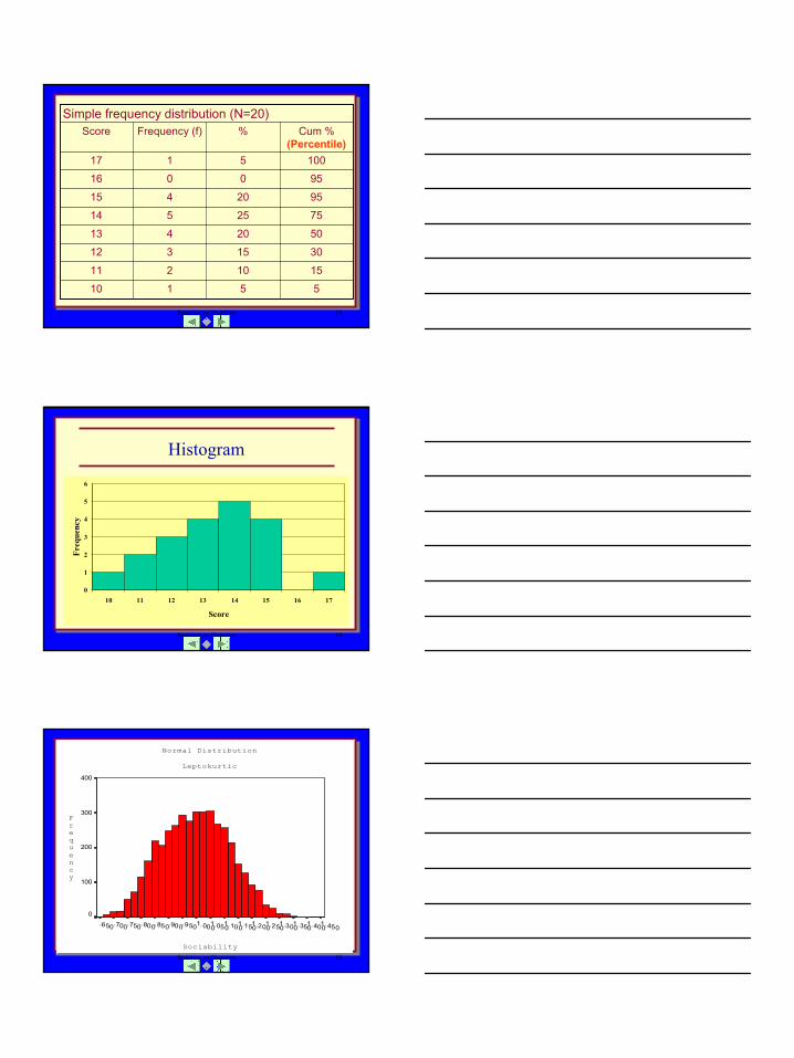
Simple frequency distribution (N=20)

1510211

55110

3015312

5020413

7525514

9520415

950016

1005117

Cum %(Percentile)

%Frequency (f)Score


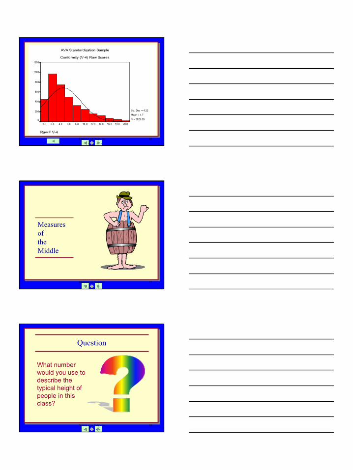
Histogram

0

1

2

3

4

5

6

10 11 12 13 14 15 16 17

Score

Freq

uenc

y


Sociability

1.4501.400

1.3501.300

1.2501.200

1.1501.100

1.0501.000

.950.900.850.800.750.700.650

Normal Distribution

Leptokurtic

Frequency

400

300

200

100

0

6


Raw F V-4

20.018.016.014.012.010.08.06.04.02.00.0

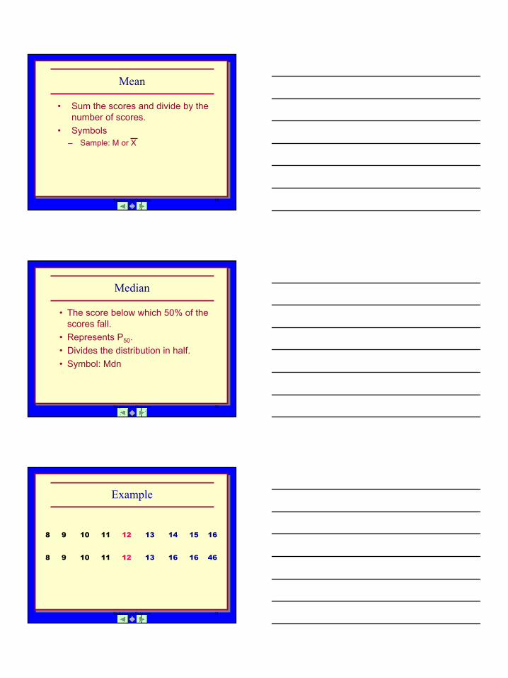
AVA Standardization Sample

Conformity (V-4) Raw Scores1200

1000

800

600

400

200

0

Std. Dev = 4.22 Mean = 4.7N = 3629.00


MeasuresoftheMiddle


Question

What number would you use to describe the typical height of people in this class?

7


Mean

• Sum the scores and divide by the number of scores.

• Symbols– Sample: M or X


Median

• The score below which 50% of the scores fall.

• Represents P50.• Divides the distribution in half.• Symbol: Mdn


Example

8 9 10 11 12 13 14 15 16

8 9 10 11 12 13 16 16 46

8


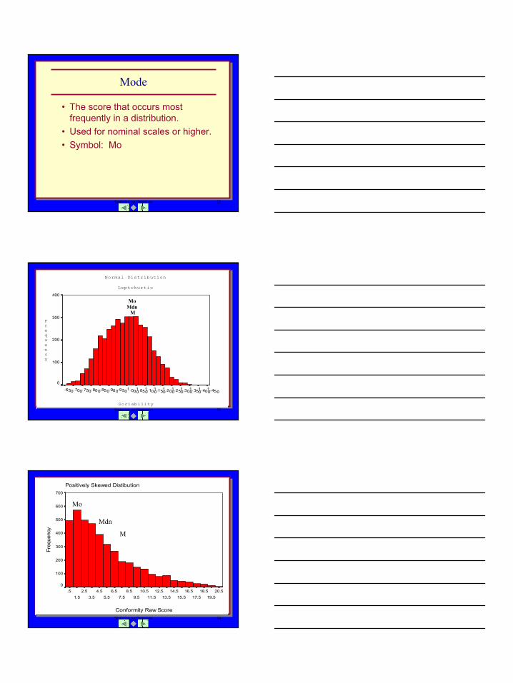
Mode

• The score that occurs most frequently in a distribution.

• Used for nominal scales or higher.• Symbol: Mo

Statistics, an Overview 23Sociability

1.4501.400

1.3501.300

1.2501.200

1.1501.100

1.0501.000

.950.900.850.800.750.700.650

Normal Distribution

Leptokurtic

Frequency

400

300

200

100

0

MoMdn

M


Conformity Raw Score

20.519.5

18.517.5

16.515.5

14.513.5

12.511.5

10.59.5

8.57.5

6.55.5

4.53.5

2.51.5

.5

Positively Skewed Distibution

Freq

uenc

y

700

600

500

400

300

200

100

0

Mo

Mdn

M

9


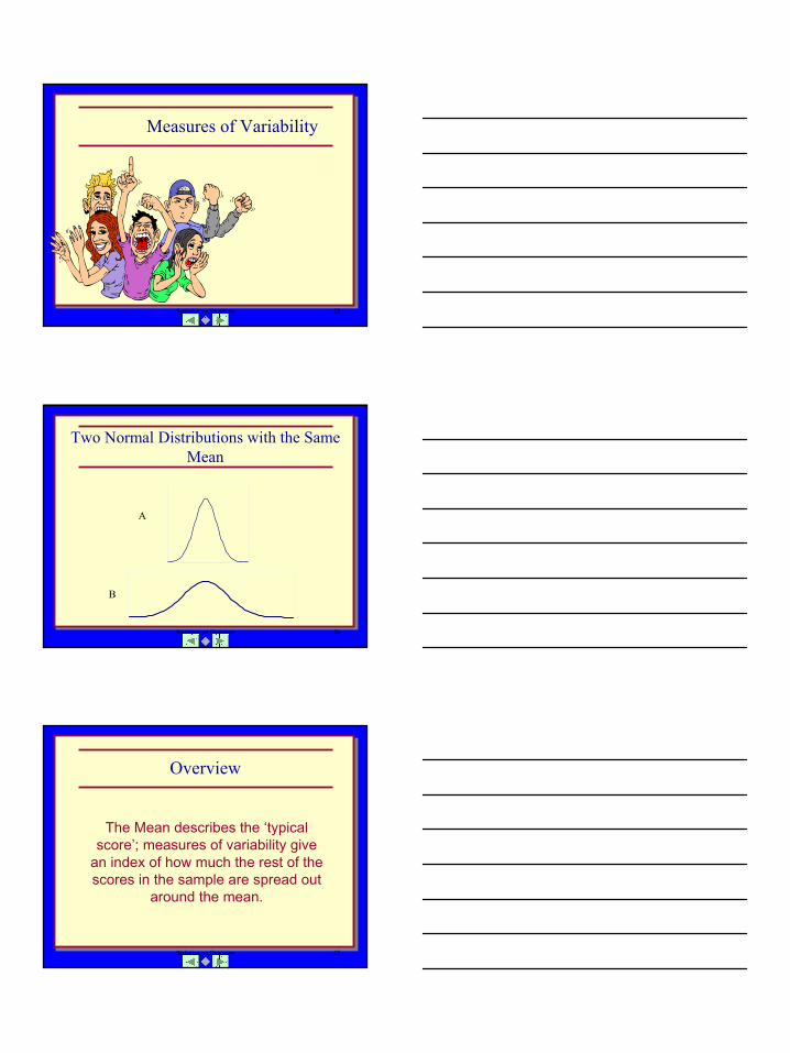
Measures of Variability


Two Normal Distributions with the Same Mean

A

B


Overview

The Mean describes the ‘typical score’; measures of variability give

an index of how much the rest of the scores in the sample are spread out

around the mean.

10


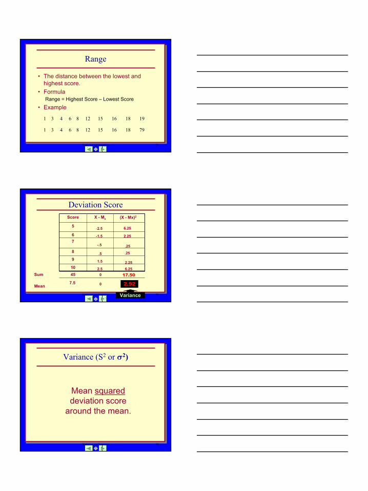
Range

• The distance between the lowest and highest score.

• FormulaRange = Highest Score – Lowest Score

• Example

1 3 4 6 8 12 15 16 18 19

1 3 4 6 8 12 15 16 18 79


Deviation Score

Mean

Sum 4510

9

76

5

8

X - MxScore

17.50

2.92

-2.5

-1.5

-.5

2.5

1.5

.5

6.25

2.25

6.252.25

.25

.25

0

0

(X - Mx)2

7.5

Variance


Variance (S2 or σ2)

Mean squareddeviation score

around the mean.

11


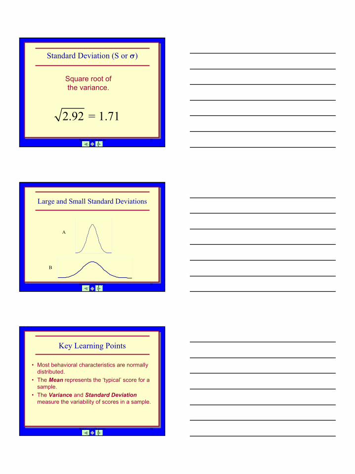
Standard Deviation (S or σ)

Square root of the variance.

2.92 = 1.71


Large and Small Standard Deviations

A

B


Key Learning Points

• Most behavioral characteristics are normally distributed.

• The Mean represents the ‘typical’ score for a sample.

• The Variance and Standard Deviationmeasure the variability of scores in a sample.

12


InferentialStatistics


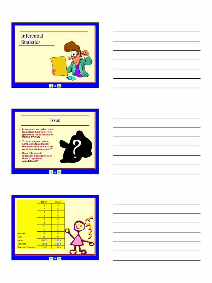
Issue

• In research we collect data from SAMPLES and try to generalize those results to POPULATIONS.

• To what degree does a sample mean representthe population to which we want to make inferences?

• Does this sample represent population A or does it represent population B?


1.8082.357Standard Deviation3.2685.554Variance5.8756.875Mean

4755Sum88Number57411436868958756

M&MRaisin

13


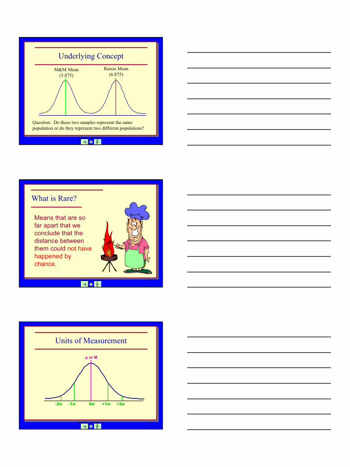
Underlying Concept

Question: Do these two samples represent the same population or do they represent two different populations?

M&M Mean (5.875)

Raisin Mean (6.875)


What is Rare?

Means that are so far apart that we conclude that the distance between them could not have happened by chance.


Units of Measurement

µ or M

+1σ-1σ +2σ-2σ 0σ

14


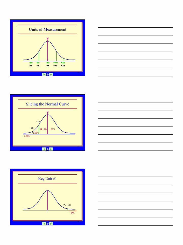
Units of Measurement

M

+1σ-1σ +2σ-2σ 0σ+1z-1z +2z-2z 0z


Slicing the Normal Curve

M

50%34.13%

13.59%2.28%

-1z

-2z


Key Unit #1

5%

Z=1.64

15


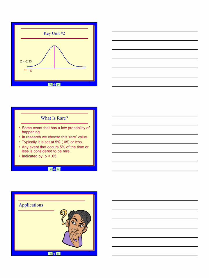
Key Unit #2

1%

Z = -2.33


What Is Rare?

• Some event that has a low probability of happening.

• In research we choose this ‘rare’ value.• Typically it is set at 5% (.05) or less.• Any event that occurs 5% of the time or

less is considered to be rare.• Indicated by: p < .05


Applications

16


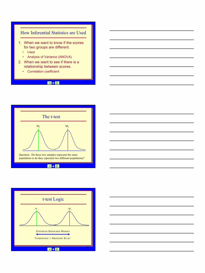
How Inferential Statistics are Used

1. When we want to know if the scores for two groups are different.

• t-test• Analysis of Variance (ANOVA)

2. When we want to see if there is a relationship between scores.

• Correlation coefficient


The t-test

Question: Do these two samples represent the same population or do they represent two different populations?

M1 M2


t-test Logic

1M 2M

Distance Between Means

Treatment + Random Error

17


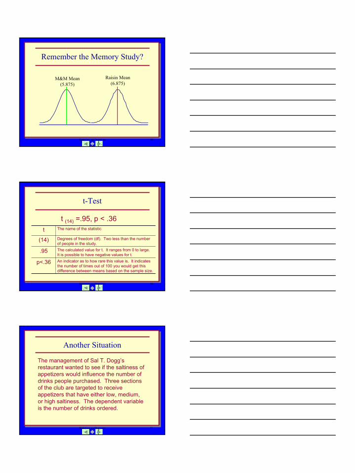
Remember the Memory Study?

M&M Mean (5.875)

Raisin Mean (6.875)


t-Test

t (14) =.95, p < .36

An indicator as to how rare this value is. It indicates the number of times out of 100 you would get this difference between means based on the sample size.

p<.36

The calculated value for t. It ranges from 0 to large. It is possible to have negative values for t.

.95

Degrees of freedom (df). Two less than the number of people in the study.

(14)

The name of the statistict


Another Situation

The management of Sal T. Dogg’srestaurant wanted to see if the saltiness of appetizers would influence the number of drinks people purchased. Three sections of the club are targeted to receive appetizers that have either low, medium, or high saltiness. The dependent variable is the number of drinks ordered.

18


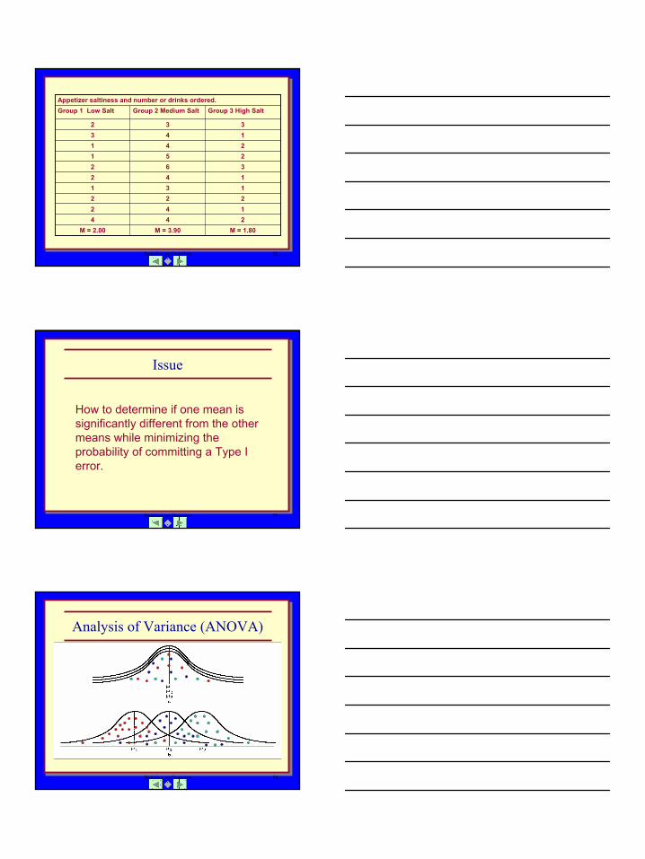
Appetizer saltiness and number or drinks ordered.

M = 1.80M = 3.90M = 2.00244142222131142362251241143332

Group 3 High SaltGroup 2 Medium SaltGroup 1 Low Salt


Issue

How to determine if one mean is significantly different from the other means while minimizing the probability of committing a Type I error.


Analysis of Variance (ANOVA)

19


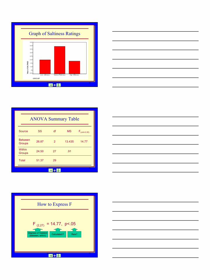
Graph of Saltiness Ratings

GROUP

High SaltinessMedium SaltinessLow saltiness

Mea

n of

SAL

TINE

S

4.5

4.0

3.5

3.0

2.5

2.0

1.5

1.0

.5

0.0


ANOVA Summary Table

2951.37Total

.912724.50Within Groups

14.7713.435226.87Between Groups

F(crit=3.35)MSdfSSSource


How to Express F

F (2,27) = 14.77, p<.05

Calculated FDegrees of freedom(between, within) Rare?

20


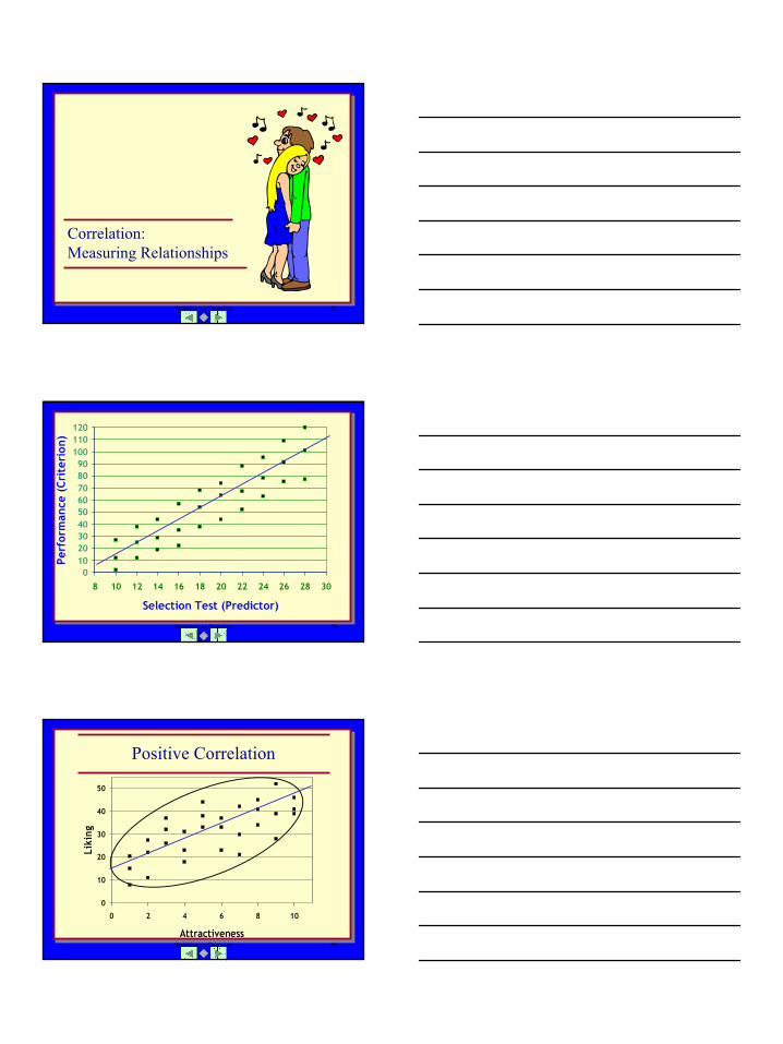
Correlation:Measuring Relationships


0102030405060708090

100110120

8 10 12 14 16 18 20 22 24 26 28 30

Selection Test (Predictor)

Perf

orm

ance

(Cr

iter

ion)


Positive Correlation

0

10

20

30

40

50

0 2 4 6 8 10

Attractiveness

Liki

ng

21


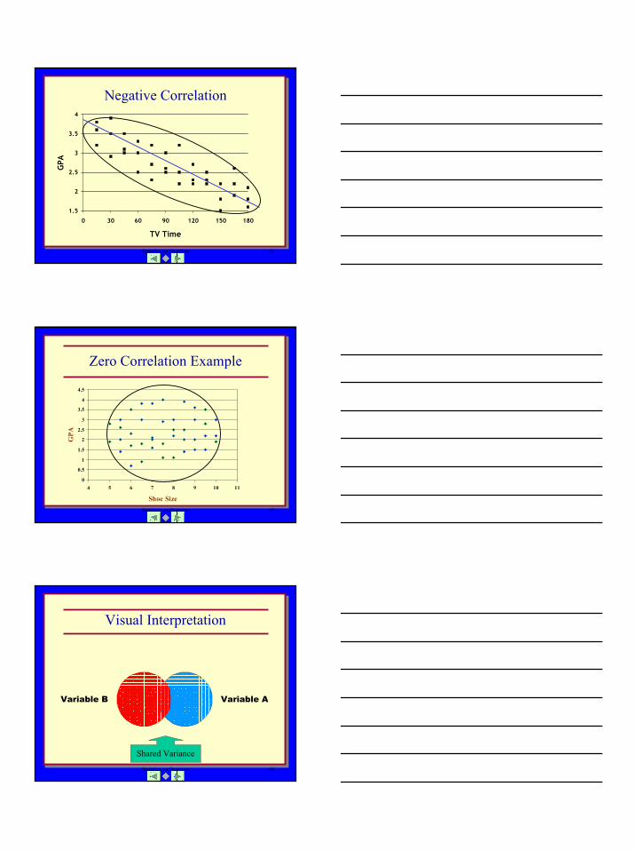
Negative Correlation

1.5

2

2.5

3

3.5

4

0 30 60 90 120 150 180

TV Time

GPA


0

0.5

1

1.5

2

2.5

3

3.5

4

4.5

4 5 6 7 8 9 10 11

Shoe Size

GPA

Zero Correlation Example


Visual Interpretation

Shared Variance

Variable AVariable B

22


Relationship Strength

Strong Moderate Weak


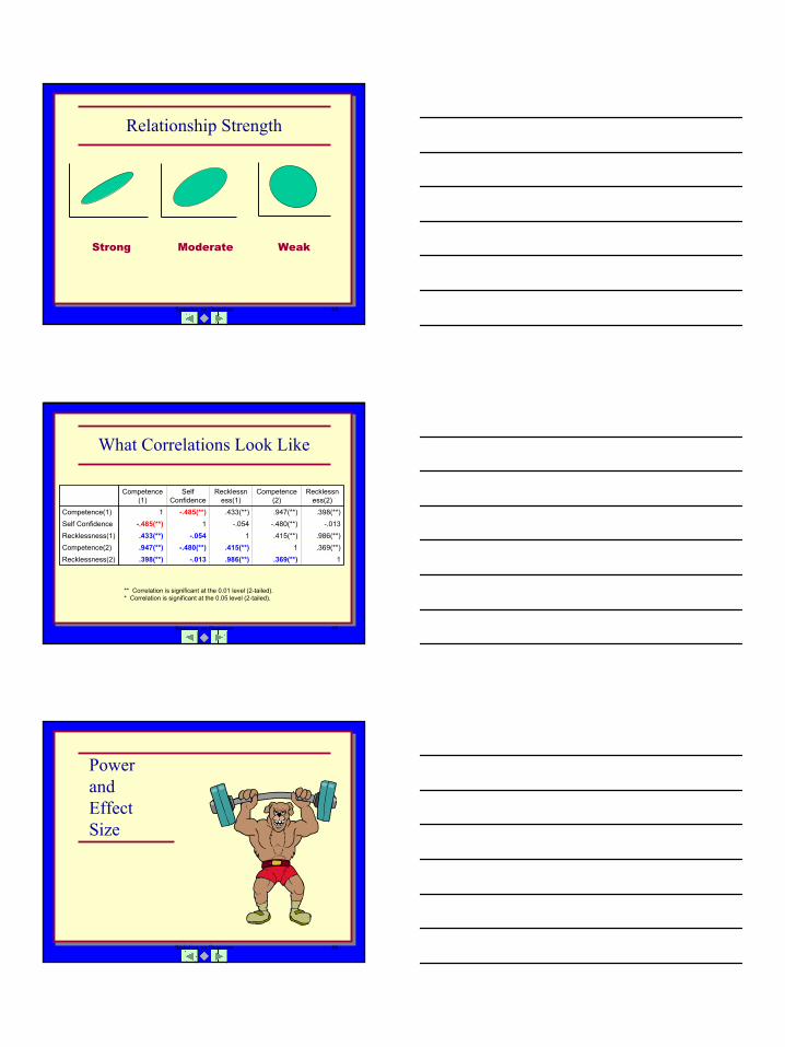
What Correlations Look Like

1.369(**).986(**)-.013.398(**)Recklessness(2).369(**)1.415(**)-.480(**).947(**)Competence(2).986(**).415(**)1-.054.433(**)Recklessness(1)

-.013-.480(**)-.0541-.485(**)Self Confidence.398(**).947(**).433(**)-.485(**)1Competence(1)

Recklessness(2)

Competence(2)

Recklessness(1)

Self Confidence

Competence(1)

** Correlation is significant at the 0.01 level (2-tailed).* Correlation is significant at the 0.05 level (2-tailed).


Power and Effect Size

23


Effect Size

1. How strong was the treatment?2. How strong is the relationship?


Power

The ability of the statistical procedure to detect the effect

being measured.


Hypotheses

24


What is hypothesis testing?

A set of logical and statistical guidelines used to make

inferential decisions from sample statistics to population

characteristics.


Types of Hypotheses

• Research hypothesis.• Logical hypotheses.

– Null hypothesis (Ho).– Alternative hypothesis (Ha).

• Statistical hypothesis.


Research Hypothesis

Statement in words as to what the investigator expects to find.

Example.

Students who drink caffeine will be able to memorize information faster than students who do not drink caffeine.

25


Logical Hypotheses

Null Hypothesis (Ho).Statement that the treatment does not have the expected effect.

Alternative Hypothesis (Ha).Statement that the treatment had the expected effect.


Characteristics of the Logical Hypotheses

1. They are mutually exclusive.

2. They are mutually exhaustive.


How they fit together

Research hypothesis.

Students who drink caffeine will be able to memorize information faster than students who do not drink caffeine.

26


How They Fit Together #2

• HoStudents who drink caffeine will not be able to memorize information faster than people who do not drink caffeine.

• Non-caffeine and caffeine drinkers are the same.• Non-caffeine drinkers are faster.

• HaStudents who drink caffeine will memorize information faster than those who do not drink caffeine.


Caffeine Example, AGAIN!

Ha: Mcaffeine < Mno caffeine

Ho: Mcaffeine = Mno caffeine

or

Mcaffeine > Mno affeine


Decision Making Criteria

1. We make statistical inferences based on the probability that the results may or may nothave happened by chance.

2. Since we are dealing with sampling error there is always a possibility that data we collect could have happened by chance.

3. Our model for making this decision is founded on the normal distribution.

27


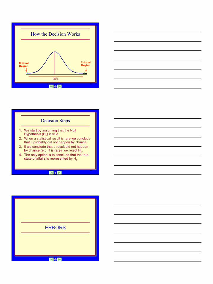
How the Decision Works

95%

CriticalRegion

CriticalRegion


Decision Steps

1. We start by assuming that the Null Hypothesis (Ho) is true.

2. When a statistical result is rare we conclude that it probably did not happen by chance.

3. If we conclude that a result did not happen by chance (e.g. it is rare), we reject Ho.

4. The only option is to conclude that the true state of affairs is represented by Ha.

ERRORS

28


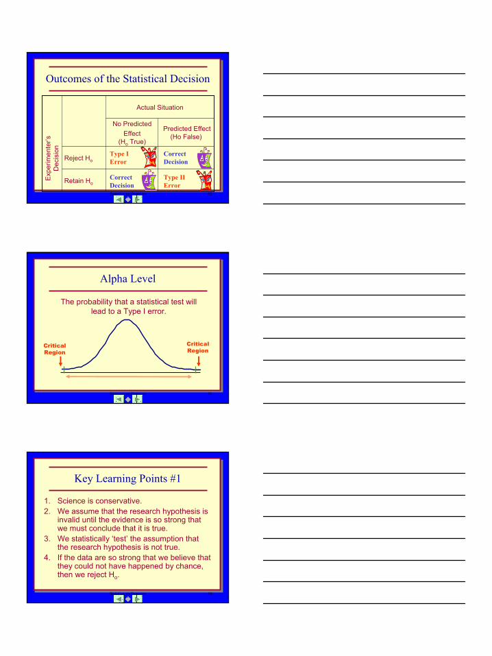
Outcomes of the Statistical Decision

Retain Ho

Reject Ho

Predicted Effect(Ho False)

No PredictedEffect

(Ho True)

Actual Situation

Exp

erim

ente

r’sD

ecis

ion

Correct Decision

Correct Decision

Type IError

Type IIError


Alpha Level

The probability that a statistical test will lead to a Type I error.

CriticalRegion

CriticalRegion


Key Learning Points #1

1. Science is conservative.2. We assume that the research hypothesis is

invalid until the evidence is so strong that we must conclude that it is true.

3. We statistically ‘test’ the assumption that the research hypothesis is not true.

4. If the data are so strong that we believe that they could not have happened by chance, then we reject Ho.

29


Key Learning Points #2

5. Since our decisions are based on probability theory not absolute surety, we can make mistakes.

6. The probability of concluding that the research hypothesis is correct when it isn’t (rejecting Ho when it is true) is represented by alpha (").

7. The probability of failing to find a result when there is one is represented by beta ($).


THE END

Documents

What We Will Cover in This Section