What Will the Next Real Estate Cycle Look Like · in the same cycle and that the residential real estate market and commercial real estate market are closely ... New commercial properties

Testimony of

Glenn R. Mueller, Ph.D.

Before the

Subcommittee on Financial Institutions and Consumer Credit

Of the

Committee on Financial Services

United States House of Representatives

September 14, 2006

2

Real Estate Space Market Cycles By Glenn R. Mueller, Ph.D.

Professor - University of Denver Franklin L. Burns School of Real Estate & Construction Management

& Real Estate Investment Strategist - Dividend Capital Group, Inc.

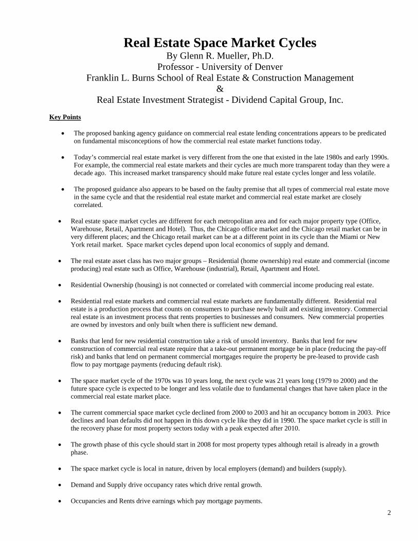
Key Points

• The proposed banking agency guidance on commercial real estate lending concentrations appears to be predicated on fundamental misconceptions of how the commercial real estate market functions today.

• Today’s commercial real estate market is very different from the one that existed in the late 1980s and early 1990s.

For example, the commercial real estate markets and their cycles are much more transparent today than they were a decade ago. This increased market transparency should make future real estate cycles longer and less volatile.

• The proposed guidance also appears to be based on the faulty premise that all types of commercial real estate move

in the same cycle and that the residential real estate market and commercial real estate market are closely correlated.

• Real estate space market cycles are different for each metropolitan area and for each major property type (Office,

Warehouse, Retail, Apartment and Hotel). Thus, the Chicago office market and the Chicago retail market can be in very different places; and the Chicago retail market can be at a different point in its cycle than the Miami or New York retail market. Space market cycles depend upon local economics of supply and demand.

• The real estate asset class has two major groups – Residential (home ownership) real estate and commercial (income

producing) real estate such as Office, Warehouse (industrial), Retail, Apartment and Hotel. • Residential Ownership (housing) is not connected or correlated with commercial income producing real estate.

• Residential real estate markets and commercial real estate markets are fundamentally different. Residential real

estate is a production process that counts on consumers to purchase newly built and existing inventory. Commercial real estate is an investment process that rents properties to businesses and consumers. New commercial properties are owned by investors and only built when there is sufficient new demand.

• Banks that lend for new residential construction take a risk of unsold inventory. Banks that lend for new

construction of commercial real estate require that a take-out permanent mortgage be in place (reducing the pay-off risk) and banks that lend on permanent commercial mortgages require the property be pre-leased to provide cash flow to pay mortgage payments (reducing default risk).

• The space market cycle of the 1970s was 10 years long, the next cycle was 21 years long (1979 to 2000) and the

future space cycle is expected to be longer and less volatile due to fundamental changes that have taken place in the commercial real estate market place.

• The current commercial space market cycle declined from 2000 to 2003 and hit an occupancy bottom in 2003. Price

declines and loan defaults did not happen in this down cycle like they did in 1990. The space market cycle is still in the recovery phase for most property sectors today with a peak expected after 2010.

• The growth phase of this cycle should start in 2008 for most property types although retail is already in a growth

phase.

• The space market cycle is local in nature, driven by local employers (demand) and builders (supply).

• Demand and Supply drive occupancy rates which drive rental growth.

• Occupancies and Rents drive earnings which pay mortgage payments.

3

• The severe downturn that occurred in the commercial real estate market during the late 1980s and early 1990s was

triggered by factors that are not present in today's environment, such as (i) changes to the Internal Revenue Code in the 1980s that encouraged people to make investments in tax shelter commercial real estate that were not based on the underlying profitability of the project, and (ii) the expansion of lending powers of thrifts that allowed them to make commercial real estate loans for the first time, and thus introduced numerous inexperienced lenders into the market. These factors led to overbuilding.

• The potentiality for a commercial real estate bubble has significantly decreased because of the introduction of Public

Market Capital from Real Estate Investment Trusts (REITs) and Commercial Mortgage Backed Securities (CMBS). This introduction of public capital has changed the dynamics of the space market cycle.

• Real Estate Space Markets can move differently from Real Estate Capital Markets.

Purpose of This Written Testimony Earlier this year, the federal banking agencies issued proposed guidance entitled “Concentrations in Commercial Real Estate Lending, Sound Risk Management Practices” (the “Guidance”). The proposed Guidance sets forth certain thresholds for assessing whether an institution has commercial real estate loan concentrations that would trigger heightened risk management practices and potentially higher capital requirements. After analyzing the proposed Guidance, it appears that it is predicated on fundamental misconceptions of how the commercial real estate market functions today. These misconceptions seem to be based on the assumption that this market has not witnessed fundamental changes over the last two decades. Simply stated, today’s commercial real estate market is very different from the one that existed in the late 1980’s and early 1990’s. For example, the commercial real estate markets and their cycles are much more transparent today than they were a decade ago. This increased transparency allows investors, developers and lenders to react much more quickly to market risks and substantially reduces the potential for overbuilding. This increased market transparency should make future real estate cycles longer and less volatile.

Another misconception underlying the proposed Guidance is the apparent belief by the banking agencies that all types of commercial real estate (Office, Warehouse, Retail, Apartment and Hotel) move in the same cycle and, thus, bear the same risk. This is simply not true. Commercial real estate cycles are different for each metropolitan area and for each major property type. This is shown in the attached Market Cycle report (Appendix A). The Guidance’s one-size-fits-all approach does not take into account diversification by geography and product type.

The definition of commercial real estate in the proposed Guidance also appears to be based on the misconception that the residential real estate market and commercial real estate market are correlated to such an extent that certain types of residential loans should be included within the definition of commercial real estate for purposes of the proposed Guidance. This is a faulty premise because the commercial real estate market and the residential real estate market are fundamentally different.

Commercial real estate is a necessary and important part of economic growth. In order to avoid any potential unintended consequences, the bank regulatory approach to commercial real estate lending must be predicated on an accurate understanding of today’s commercial real estate market environment. The purpose of this written testimony is to set forth the changes that have occurred in the commercial real estate market over the last two decades in order to address the misconceptions upon which the proposed Guidance appears to be based.

4

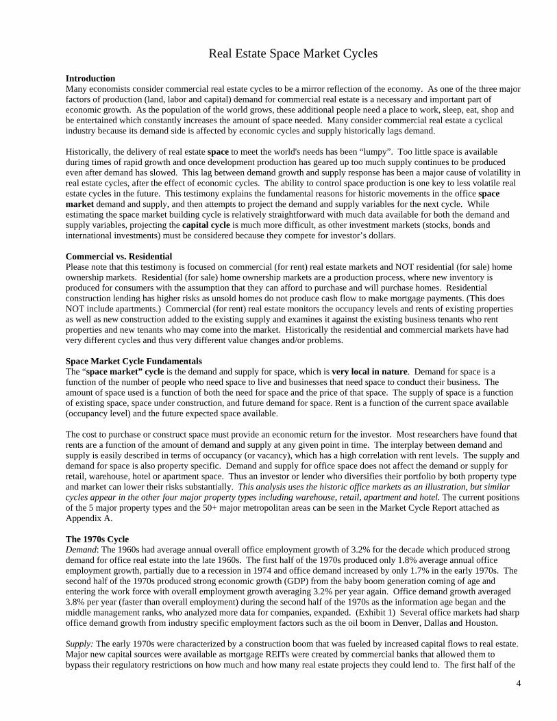
Real Estate Space Market Cycles Introduction Many economists consider commercial real estate cycles to be a mirror reflection of the economy. As one of the three major factors of production (land, labor and capital) demand for commercial real estate is a necessary and important part of economic growth. As the population of the world grows, these additional people need a place to work, sleep, eat, shop and be entertained which constantly increases the amount of space needed. Many consider commercial real estate a cyclical industry because its demand side is affected by economic cycles and supply historically lags demand. Historically, the delivery of real estate space to meet the world's needs has been “lumpy”. Too little space is available during times of rapid growth and once development production has geared up too much supply continues to be produced even after demand has slowed. This lag between demand growth and supply response has been a major cause of volatility in real estate cycles, after the effect of economic cycles. The ability to control space production is one key to less volatile real estate cycles in the future. This testimony explains the fundamental reasons for historic movements in the office space market demand and supply, and then attempts to project the demand and supply variables for the next cycle. While estimating the space market building cycle is relatively straightforward with much data available for both the demand and supply variables, projecting the capital cycle is much more difficult, as other investment markets (stocks, bonds and international investments) must be considered because they compete for investor’s dollars. Commercial vs. Residential Please note that this testimony is focused on commercial (for rent) real estate markets and NOT residential (for sale) home ownership markets. Residential (for sale) home ownership markets are a production process, where new inventory is produced for consumers with the assumption that they can afford to purchase and will purchase homes. Residential construction lending has higher risks as unsold homes do not produce cash flow to make mortgage payments. (This does NOT include apartments.) Commercial (for rent) real estate monitors the occupancy levels and rents of existing properties as well as new construction added to the existing supply and examines it against the existing business tenants who rent properties and new tenants who may come into the market. Historically the residential and commercial markets have had very different cycles and thus very different value changes and/or problems. Space Market Cycle Fundamentals The “space market” cycle is the demand and supply for space, which is very local in nature. Demand for space is a function of the number of people who need space to live and businesses that need space to conduct their business. The amount of space used is a function of both the need for space and the price of that space. The supply of space is a function of existing space, space under construction, and future demand for space. Rent is a function of the current space available (occupancy level) and the future expected space available. The cost to purchase or construct space must provide an economic return for the investor. Most researchers have found that rents are a function of the amount of demand and supply at any given point in time. The interplay between demand and supply is easily described in terms of occupancy (or vacancy), which has a high correlation with rent levels. The supply and demand for space is also property specific. Demand and supply for office space does not affect the demand or supply for retail, warehouse, hotel or apartment space. Thus an investor or lender who diversifies their portfolio by both property type and market can lower their risks substantially. This analysis uses the historic office markets as an illustration, but similar cycles appear in the other four major property types including warehouse, retail, apartment and hotel. The current positions of the 5 major property types and the 50+ major metropolitan areas can be seen in the Market Cycle Report attached as Appendix A. The 1970s Cycle Demand: The 1960s had average annual overall office employment growth of 3.2% for the decade which produced strong demand for office real estate into the late 1960s. The first half of the 1970s produced only 1.8% average annual office employment growth, partially due to a recession in 1974 and office demand increased by only 1.7% in the early 1970s. The second half of the 1970s produced strong economic growth (GDP) from the baby boom generation coming of age and entering the work force with overall employment growth averaging 3.2% per year again. Office demand growth averaged 3.8% per year (faster than overall employment) during the second half of the 1970s as the information age began and the middle management ranks, who analyzed more data for companies, expanded. (Exhibit 1) Several office markets had sharp office demand growth from industry specific employment factors such as the oil boom in Denver, Dallas and Houston. Supply: The early 1970s were characterized by a construction boom that was fueled by increased capital flows to real estate. Major new capital sources were available as mortgage REITs were created by commercial banks that allowed them to bypass their regulatory restrictions on how much and how many real estate projects they could lend to. The first half of the

5

1970s saw total office space construction increase by an average 5.6% per year. The recession of 1974 slowed GDP and employment growth, and the office markets down-cycled and crashed in 1974 and 1975. Many construction loans defaulted and never converted to permanent loan status. New “empty buildings” were foreclosed upon and held by mortgage REITs whose stock values plummeted from a peak NAREIT Index of 112.39 in January 1973 to a low 39.09 in December 1974, when the mortgage REITs could not make their dividend payments. The REIT industry, which had begun in 1960, grew to around $10 billion in market capitalization and subsequently shrunk to $2 billion in 1975. The flow of capital to real estate construction shut down and new space growth slowed to 1.5% in 1976 then recovered to a more moderate 3.2% average in the second half of the 1970s. The early 1970s period of overbuilding was initiated due to surprisingly strong demand growth in the late 1960s that allowed the capital markets to “sell a story” about mortgage REITs to public investors. Oversupply pushed office occupancies to a bottom in 1975 (Exhibit 5). After the crash, the public market branded mortgage REITs as “bad and high risk” and this mortgage REIT branding still exists today in the minds of many investors. Exhibit 1 shows the high rate of growth in supply and relatively low rate of growth in demand in the first half of the 1970s causing a down cycle, while the second half was characterized by stronger demand growth than supply growth allowing recovery and then expansion to take place.

Exhibit 1

1970s Office Demand & Supply

0%

2%

4%

6%

8%

1970

1971

1972

1973

1974

1975

1976

1977

1978

1979

Demand Supply

Source: FW Dodge, CB Commercial, BLS, Mueller

Oversupply Years Baby Boomers Go To Work

The 1980s Cycle Demand: The U.S. began to move into the information age in the late 1970s and economic prosperity coupled with very strong white-collar employment growth from the baby boom generation helped create a 4.7% annual average GDP growth rate for the decade. A recession in 1981 was caused by high government debt pushing interest rates up to the high teens (10 year treasuries reached 15% in 1981) which caused construction spending and consumer spending to slow. After 1981 strong government spending, continued strong employment growth and the dawn of the personal computer age helped GDP to maintain strong growth rates throughout the rest of the 1980s. Employment growth averaged 2.8% per year for the decade while office demand grew an average yearly rate of 3.6% for the decade. Supply: Real estate was a private marketplace in the 1980s, with little information available about construction starts versus future demand. In addition, thrifts were allowed to lend on commercial real estate where they had no previous experience. There were few researchers or national level data sources at the beginning of the decade and only a handful at the end of the decade. Data was provided by commercial brokers whose motivation was to close deals. Computers made 10 year investment projections a new way of life, but the standard occupancy assumption was 95% for each year going forward even when many market occupancy rates were declining. Supply was growing at an average 7.7% per year during the decade which was double demand growth, thus the occupancy rate was declining yearly. (Exhibit 5). The tax act of 1981 created more capital flow to real estate for tax shelters and thus more construction of tax driven (non-economic) real estate deals.

6

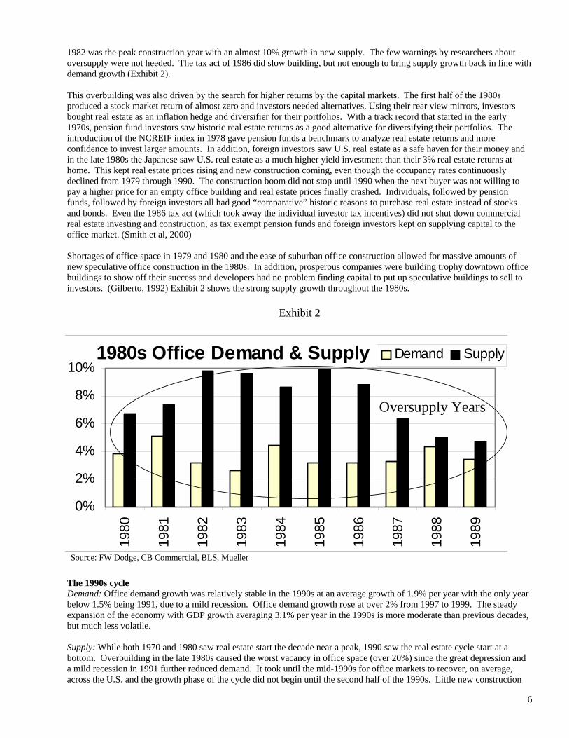
1982 was the peak construction year with an almost 10% growth in new supply. The few warnings by researchers about oversupply were not heeded. The tax act of 1986 did slow building, but not enough to bring supply growth back in line with demand growth (Exhibit 2). This overbuilding was also driven by the search for higher returns by the capital markets. The first half of the 1980s produced a stock market return of almost zero and investors needed alternatives. Using their rear view mirrors, investors bought real estate as an inflation hedge and diversifier for their portfolios. With a track record that started in the early 1970s, pension fund investors saw historic real estate returns as a good alternative for diversifying their portfolios. The introduction of the NCREIF index in 1978 gave pension funds a benchmark to analyze real estate returns and more confidence to invest larger amounts. In addition, foreign investors saw U.S. real estate as a safe haven for their money and in the late 1980s the Japanese saw U.S. real estate as a much higher yield investment than their 3% real estate returns at home. This kept real estate prices rising and new construction coming, even though the occupancy rates continuously declined from 1979 through 1990. The construction boom did not stop until 1990 when the next buyer was not willing to pay a higher price for an empty office building and real estate prices finally crashed. Individuals, followed by pension funds, followed by foreign investors all had good “comparative” historic reasons to purchase real estate instead of stocks and bonds. Even the 1986 tax act (which took away the individual investor tax incentives) did not shut down commercial real estate investing and construction, as tax exempt pension funds and foreign investors kept on supplying capital to the office market. (Smith et al, 2000) Shortages of office space in 1979 and 1980 and the ease of suburban office construction allowed for massive amounts of new speculative office construction in the 1980s. In addition, prosperous companies were building trophy downtown office buildings to show off their success and developers had no problem finding capital to put up speculative buildings to sell to investors. (Gilberto, 1992) Exhibit 2 shows the strong supply growth throughout the 1980s.

Exhibit 2


0%

2%

4%

6%

8%

10%

1980

1981

1982

1983

1984

1985

1986

1987

1988

1989

Demand Supply


Oversupply Years

The 1990s cycle Demand: Office demand growth was relatively stable in the 1990s at an average growth of 1.9% per year with the only year below 1.5% being 1991, due to a mild recession. Office demand growth rose at over 2% from 1997 to 1999. The steady expansion of the economy with GDP growth averaging 3.1% per year in the 1990s is more moderate than previous decades, but much less volatile. Supply: While both 1970 and 1980 saw real estate start the decade near a peak, 1990 saw the real estate cycle start at a bottom. Overbuilding in the late 1980s caused the worst vacancy in office space (over 20%) since the great depression and a mild recession in 1991 further reduced demand. It took until the mid-1990s for office markets to recover, on average, across the U.S. and the growth phase of the cycle did not begin until the second half of the 1990s. Little new construction

7

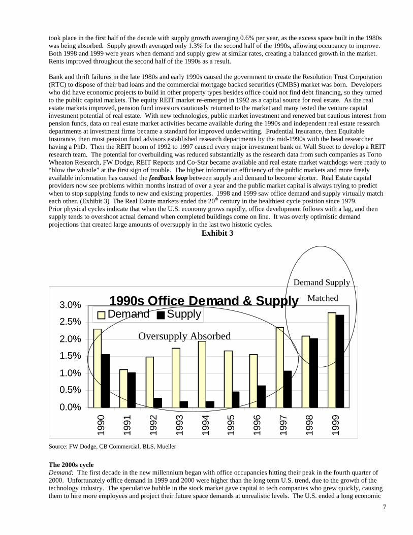
took place in the first half of the decade with supply growth averaging 0.6% per year, as the excess space built in the 1980s was being absorbed. Supply growth averaged only 1.3% for the second half of the 1990s, allowing occupancy to improve. Both 1998 and 1999 were years when demand and supply grew at similar rates, creating a balanced growth in the market. Rents improved throughout the second half of the 1990s as a result. Bank and thrift failures in the late 1980s and early 1990s caused the government to create the Resolution Trust Corporation (RTC) to dispose of their bad loans and the commercial mortgage backed securities (CMBS) market was born. Developers who did have economic projects to build in other property types besides office could not find debt financing, so they turned to the public capital markets. The equity REIT market re-emerged in 1992 as a capital source for real estate. As the real estate markets improved, pension fund investors cautiously returned to the market and many tested the venture capital investment potential of real estate. With new technologies, public market investment and renewed but cautious interest from pension funds, data on real estate market activities became available during the 1990s and independent real estate research departments at investment firms became a standard for improved underwriting. Prudential Insurance, then Equitable Insurance, then most pension fund advisors established research departments by the mid-1990s with the head researcher having a PhD. Then the REIT boom of 1992 to 1997 caused every major investment bank on Wall Street to develop a REIT research team. The potential for overbuilding was reduced substantially as the research data from such companies as Torto Wheaton Research, FW Dodge, REIT Reports and Co-Star became available and real estate market watchdogs were ready to “blow the whistle” at the first sign of trouble. The higher information efficiency of the public markets and more freely available information has caused the feedback loop between supply and demand to become shorter. Real Estate capital providers now see problems within months instead of over a year and the public market capital is always trying to predict when to stop supplying funds to new and existing properties. 1998 and 1999 saw office demand and supply virtually match each other. (Exhibit 3) The Real Estate markets ended the 20th century in the healthiest cycle position since 1979. Prior physical cycles indicate that when the U.S. economy grows rapidly, office development follows with a lag, and then supply tends to overshoot actual demand when completed buildings come on line. It was overly optimistic demand projections that created large amounts of oversupply in the last two historic cycles.

Exhibit 3


0.0%

0.5%

1.0%

1.5%

2.0%

2.5%

3.0%

1990

1991

1992

1993

1994

1995

1996

1997

1998

1999

Demand Supply


Oversupply Absorbed

Demand Supply

Matched

The 2000s cycle Demand: The first decade in the new millennium began with office occupancies hitting their peak in the fourth quarter of 2000. Unfortunately office demand in 1999 and 2000 were higher than the long term U.S. trend, due to the growth of the technology industry. The speculative bubble in the stock market gave capital to tech companies who grew quickly, causing them to hire more employees and project their future space demands at unrealistic levels. The U.S. ended a long economic

8

expansion in 2001 after the tech bubble burst. Annual office employment declined for the first time by over -1% in 2001, while office demand (absorption) declined by over -2% as firms with excess space put that space on the sub-lease market in an attempt to rent unused space to other users and reduce their costs. This demand driven downturn was different from the supply driven down cycles of the 1970s and 1980s creating a new challenge for researchers. National office employment has always been positive in past cycles, while negative net absorption has been caused by too much supply. Office supply did react quickly, declining to very low levels and allowing the market to bottom quickly and begin a recovery in 2003. Office employment has grown from 2002 to 2006 and is expected to grow over the next decade. Some of the major reasons for this continued growth include increasing demand from a globalized economy, continued technology revolution, and long term population growth. Population growth at just under 1% per year on a 300 million U.S. base translates into 2.5 million new people per year in the U.S., each year, for the next ten years. These additional people (half immigrants and half new births net of deaths) still need additional real estate to work in, shop at, sleep in, eat at, and play in. This means the U.S. will need to build one complete new city like Denver, or Phoenix each year for the next 10 years to meet space demand. While there may be small periods of recession, the long-term prospects are positive. In this cycle office employment increased by only 1.2% in 2004 and 1.4% in 2005 with a 5 year forecast of 1.5% going forward. Overall office demand (absorption) is expected to follow similar but slower growth rates of 1.3% over the second half of the 2000’s decade. (Exhibit 4) With a flourishing economy, office demand growth is expected to average around 2% in the first half of the century. Supply: Construction starts for office declined each year for the first half of the decade, declining each year to make up for the negative demand in 2001. The supply forecast average for the second half of the 2000 decade is estimated to be only 1.3% allowing occupancies to improve. (Exhibit 4) There are three principal reasons for this forecast: 1 - Public Capital Markets With public market monitoring, it will be much more difficult to justify new space without an analysis of existing competitive construction and user demand for existing space. We have already seen the public capital market reaction to potential excess supply in cities like Atlanta where many new office construction projects were stopped in 1998 when Wall Street analysts downgraded REITs and Commercial Mortgage Backed Securities (CMBS) issues that were investing in the Atlanta office and industrial markets. New office supply in Atlanta dropped from 6.4 million square feet in 1998 to 5.9 million square feet in 1999. One Atlanta-focused REIT, Weeks Corporation, experienced a 20% stock price decline when news of Atlanta oversupply was revealed in the financial press. This monitoring by the capital markets let the Atlanta market move back into balance within a year’s time, instead of going through an overbuilding boom bust cycle. The information feedback loop that is now in place is much more likely to avoid large boom bust cycles in the future, as supply will be constrained by the wider availability of market information. The REIT market saw prices fall in 1998 and 1999 when direct markets were good and the outlook was even better, because the public capital markets were more attracted to high-tech stocks. On the other hand, the CMBS market brought more capital than traditional real estate debt lenders and many feared it would support non-economic projects. But in mid-year 2000, the REIT market recovered as the tech market fell and improved in both 2001 and 2002, showing that an earnings growth focus may be correct over the long term after all. The CMBS market has performed well from 2000 through 2006 with a focus on pre-leasing and tenant credit instead of property value. 2 - Construction Constraints Constraints on building have increased over the past decades. The number of studies and approvals necessary for new construction has tripled in cost and time, over the past two decades. Environmental impact studies, traffic impact studies, storm water runoff management and other societal impacts must now be analyzed and mitigated before development approvals are given. While F.W. Dodge economists and data providers wrote about this lengthening, they were not able to prove it as the company only began keeping historic data in 1994, all previous data gathered was discarded on a regular basis. The cost of construction labor and materials has increased at high rates and construction labor was the hardest labor force in the country to find in 2000 and the first half of 2001. Therefore producing new supply takes longer and is more expensive. Development is now much more difficult than it was in previous cycles due to the up-front costs mentioned above. Many of the major developers have become long-term investors as well, by turning their companies into REITs. Capital partners for developers are now much more sophisticated than they have been in the past, requiring feasibility studies and pre-leasing prior to funding approval. 3 - Greater Transparency The real estate markets and their cycles are much more transparent than they were a decade ago. In 1990 there were a few small firms collecting market data on 20 to 30 MSAs and selling it to a few large institutional investors. Over the decade more than 30 market research firms have been started and recently they have been consolidated into a few national firms that cover as many as 60 major markets in the U.S. in the five major property types. The largest firms are F.W. Dodge (who recently merged their data products with Torto Wheaton Research), Torto Wheaton Research (a Division of CB

9

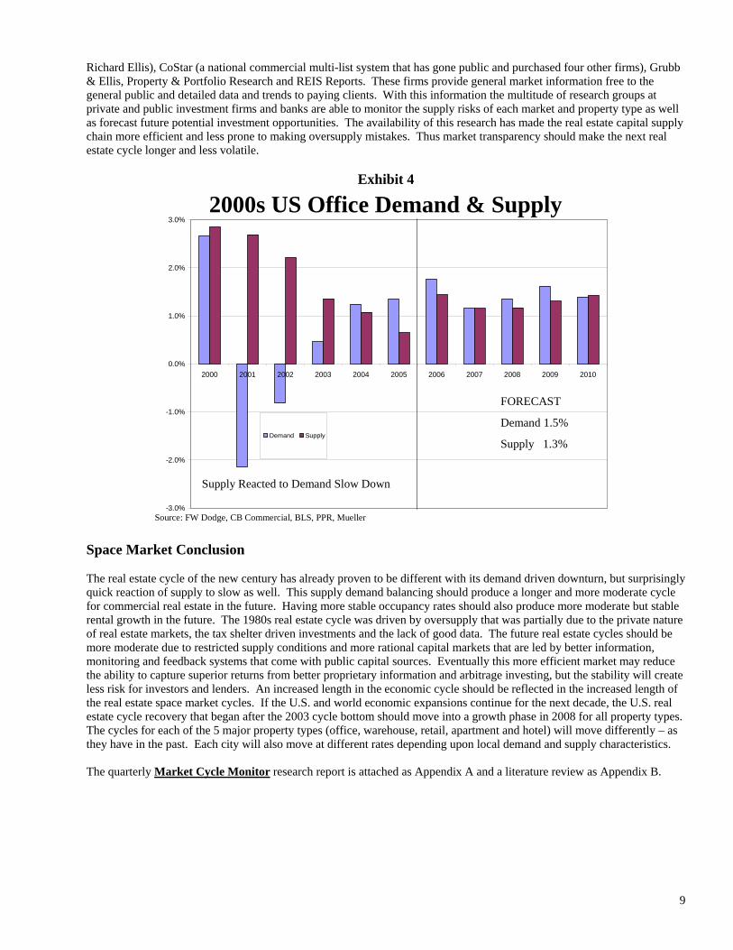
Richard Ellis), CoStar (a national commercial multi-list system that has gone public and purchased four other firms), Grubb & Ellis, Property & Portfolio Research and REIS Reports. These firms provide general market information free to the general public and detailed data and trends to paying clients. With this information the multitude of research groups at private and public investment firms and banks are able to monitor the supply risks of each market and property type as well as forecast future potential investment opportunities. The availability of this research has made the real estate capital supply chain more efficient and less prone to making oversupply mistakes. Thus market transparency should make the next real estate cycle longer and less volatile.

Exhibit 4

-3.0%

-2.0%

-1.0%

0.0%

1.0%

2.0%

3.0%

2000 2001 2002 2003 2004 2005 2006 2007 2008 2009 2010

Demand Supply

2000s US Office Demand & Supply

Source: FW Dodge, CB Commercial, BLS, PPR, Mueller

Supply Reacted to Demand Slow Down

FORECAST

Demand 1.5%

Supply 1.3%

Space Market Conclusion The real estate cycle of the new century has already proven to be different with its demand driven downturn, but surprisingly quick reaction of supply to slow as well. This supply demand balancing should produce a longer and more moderate cycle for commercial real estate in the future. Having more stable occupancy rates should also produce more moderate but stable rental growth in the future. The 1980s real estate cycle was driven by oversupply that was partially due to the private nature of real estate markets, the tax shelter driven investments and the lack of good data. The future real estate cycles should be more moderate due to restricted supply conditions and more rational capital markets that are led by better information, monitoring and feedback systems that come with public capital sources. Eventually this more efficient market may reduce the ability to capture superior returns from better proprietary information and arbitrage investing, but the stability will create less risk for investors and lenders. An increased length in the economic cycle should be reflected in the increased length of the real estate space market cycles. If the U.S. and world economic expansions continue for the next decade, the U.S. real estate cycle recovery that began after the 2003 cycle bottom should move into a growth phase in 2008 for all property types. The cycles for each of the 5 major property types (office, warehouse, retail, apartment and hotel) will move differently – as they have in the past. Each city will also move at different rates depending upon local demand and supply characteristics. The quarterly Market Cycle Monitor research report is attached as Appendix A and a literature review as Appendix B.

10

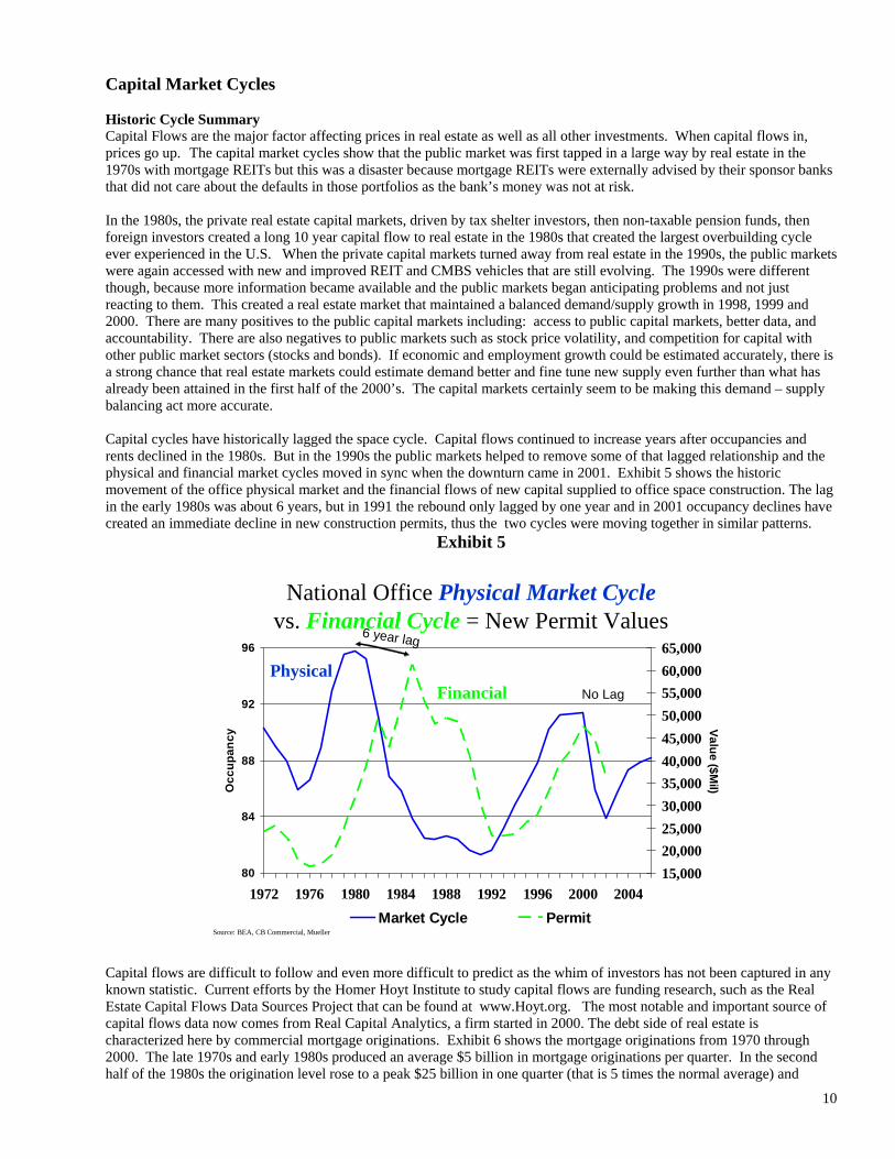
Capital Market Cycles Historic Cycle Summary Capital Flows are the major factor affecting prices in real estate as well as all other investments. When capital flows in, prices go up. The capital market cycles show that the public market was first tapped in a large way by real estate in the 1970s with mortgage REITs but this was a disaster because mortgage REITs were externally advised by their sponsor banks that did not care about the defaults in those portfolios as the bank’s money was not at risk. In the 1980s, the private real estate capital markets, driven by tax shelter investors, then non-taxable pension funds, then foreign investors created a long 10 year capital flow to real estate in the 1980s that created the largest overbuilding cycle ever experienced in the U.S. When the private capital markets turned away from real estate in the 1990s, the public markets were again accessed with new and improved REIT and CMBS vehicles that are still evolving. The 1990s were different though, because more information became available and the public markets began anticipating problems and not just reacting to them. This created a real estate market that maintained a balanced demand/supply growth in 1998, 1999 and 2000. There are many positives to the public capital markets including: access to public capital markets, better data, and accountability. There are also negatives to public markets such as stock price volatility, and competition for capital with other public market sectors (stocks and bonds). If economic and employment growth could be estimated accurately, there is a strong chance that real estate markets could estimate demand better and fine tune new supply even further than what has already been attained in the first half of the 2000’s. The capital markets certainly seem to be making this demand – supply balancing act more accurate. Capital cycles have historically lagged the space cycle. Capital flows continued to increase years after occupancies and rents declined in the 1980s. But in the 1990s the public markets helped to remove some of that lagged relationship and the physical and financial market cycles moved in sync when the downturn came in 2001. Exhibit 5 shows the historic movement of the office physical market and the financial flows of new capital supplied to office space construction. The lag in the early 1980s was about 6 years, but in 1991 the rebound only lagged by one year and in 2001 occupancy declines have created an immediate decline in new construction permits, thus the two cycles were moving together in similar patterns.

Exhibit 5

National Office Physical Market Cyclevs. Financial Cycle = New Permit Values

80

84

88

92

96

1972 1976 1980 1984 1988 1992 1996 2000 2004

Occ

upan

cy

15,00020,00025,00030,00035,00040,00045,00050,00055,00060,00065,000

Value ($Mil)

Market Cycle PermitSource: CB Commercial, Census Bureau

PhysicalFinancial

Source: BEA, CB Commercial, Mueller

6 year lag

No Lag

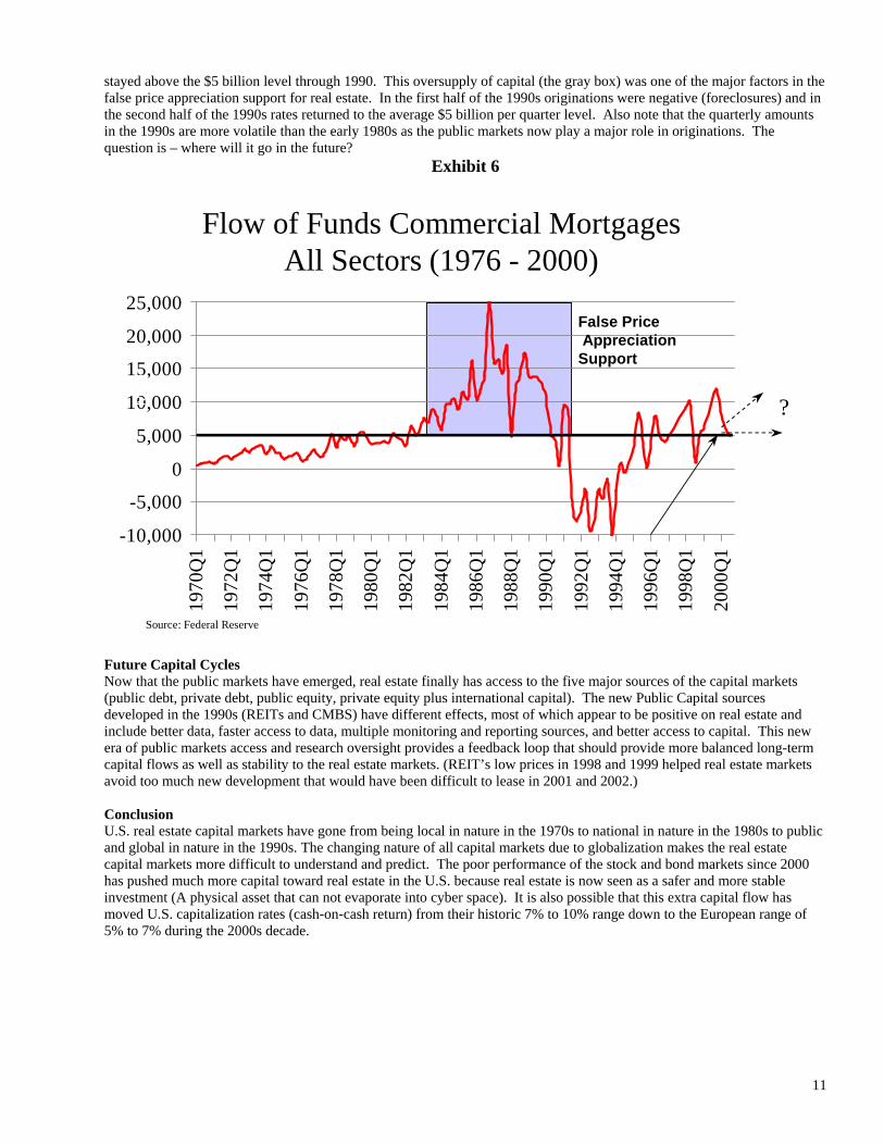
Capital flows are difficult to follow and even more difficult to predict as the whim of investors has not been captured in any known statistic. Current efforts by the Homer Hoyt Institute to study capital flows are funding research, such as the Real Estate Capital Flows Data Sources Project that can be found at www.Hoyt.org. The most notable and important source of capital flows data now comes from Real Capital Analytics, a firm started in 2000. The debt side of real estate is characterized here by commercial mortgage originations. Exhibit 6 shows the mortgage originations from 1970 through 2000. The late 1970s and early 1980s produced an average $5 billion in mortgage originations per quarter. In the second half of the 1980s the origination level rose to a peak $25 billion in one quarter (that is 5 times the normal average) and

11

stayed above the $5 billion level through 1990. This oversupply of capital (the gray box) was one of the major factors in the false price appreciation support for real estate. In the first half of the 1990s originations were negative (foreclosures) and in the second half of the 1990s rates returned to the average $5 billion per quarter level. Also note that the quarterly amounts in the 1990s are more volatile than the early 1980s as the public markets now play a major role in originations. The question is – where will it go in the future?

Exhibit 6

-10,000

-5,000

0

5,000

10,000

15,000

20,000

25,000

1970

Q1

1972

Q1

1974

Q1

1976

Q1

1978

Q1

1980

Q1

1982

Q1

1984

Q1

1986

Q1

1988

Q1

1990

Q1

1992

Q1

1994

Q1

1996

Q1

1998

Q1

2000

Q1

Flow of Funds Commercial MortgagesAll Sectors (1976 - 2000)

False PriceAppreciation

Support

?($ M

ils)

Source: Federal Reserve

Future Capital Cycles Now that the public markets have emerged, real estate finally has access to the five major sources of the capital markets (public debt, private debt, public equity, private equity plus international capital). The new Public Capital sources developed in the 1990s (REITs and CMBS) have different effects, most of which appear to be positive on real estate and include better data, faster access to data, multiple monitoring and reporting sources, and better access to capital. This new era of public markets access and research oversight provides a feedback loop that should provide more balanced long-term capital flows as well as stability to the real estate markets. (REIT’s low prices in 1998 and 1999 helped real estate markets avoid too much new development that would have been difficult to lease in 2001 and 2002.) Conclusion U.S. real estate capital markets have gone from being local in nature in the 1970s to national in nature in the 1980s to public and global in nature in the 1990s. The changing nature of all capital markets due to globalization makes the real estate capital markets more difficult to understand and predict. The poor performance of the stock and bond markets since 2000 has pushed much more capital toward real estate in the U.S. because real estate is now seen as a safer and more stable investment (A physical asset that can not evaporate into cyber space). It is also possible that this extra capital flow has moved U.S. capitalization rates (cash-on-cash return) from their historic 7% to 10% range down to the European range of 5% to 7% during the 2000s decade.

12

APPENDIX A

13

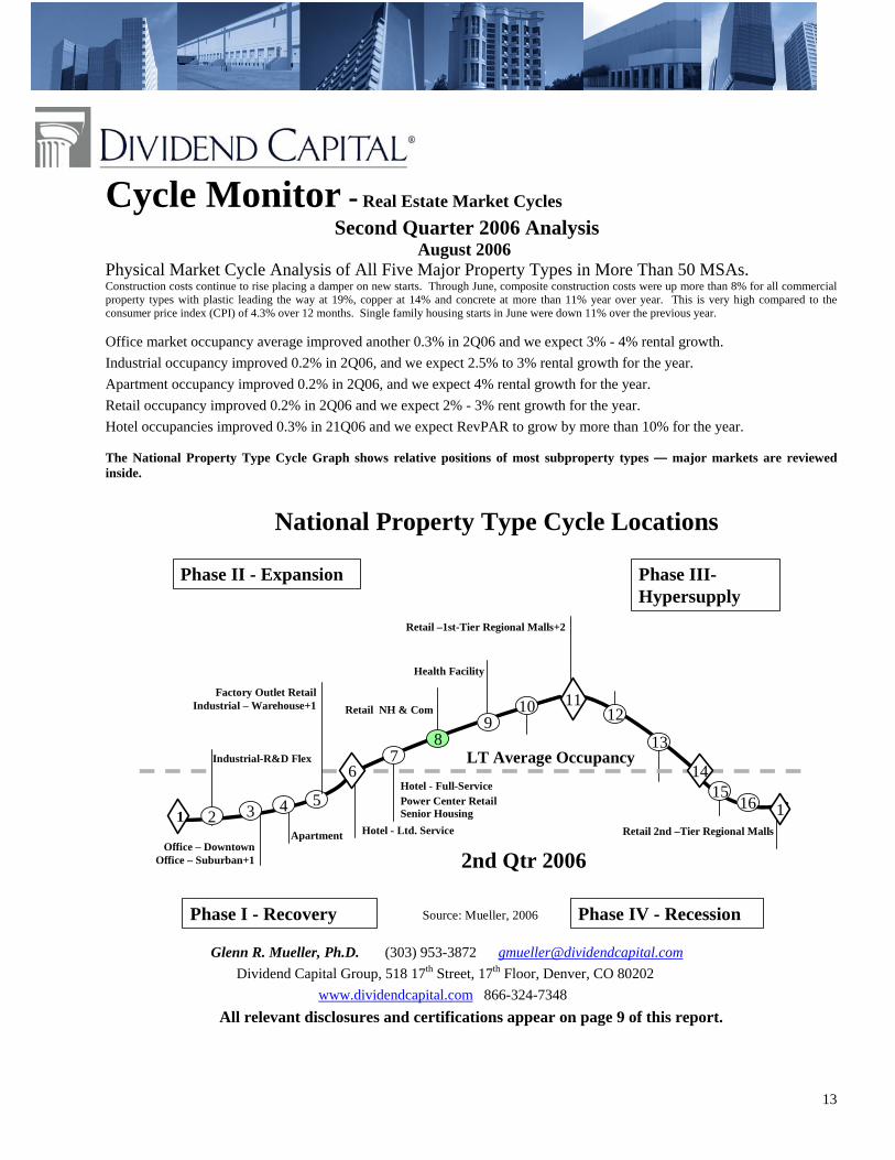
Cycle Monitor - Real Estate Market Cycles Second Quarter 2006 Analysis

August 2006 Physical Market Cycle Analysis of All Five Major Property Types in More Than 50 MSAs. Construction costs continue to rise placing a damper on new starts. Through June, composite construction costs were up more than 8% for all commercial property types with plastic leading the way at 19%, copper at 14% and concrete at more than 11% year over year. This is very high compared to the consumer price index (CPI) of 4.3% over 12 months. Single family housing starts in June were down 11% over the previous year.

Office market occupancy average improved another 0.3% in 2Q06 and we expect 3% - 4% rental growth. Industrial occupancy improved 0.2% in 2Q06, and we expect 2.5% to 3% rental growth for the year. Apartment occupancy improved 0.2% in 2Q06, and we expect 4% rental growth for the year. Retail occupancy improved 0.2% in 2Q06 and we expect 2% - 3% rent growth for the year. Hotel occupancies improved 0.3% in 21Q06 and we expect RevPAR to grow by more than 10% for the year. The National Property Type Cycle Graph shows relative positions of most subproperty types — major markets are reviewed inside.

Retail 2nd –Tier Regional Malls

National Property Type Cycle Locations

2nd Qtr 2006

LT Average Occupancy

Source: Mueller, 2006

Phase II - Expansion

Phase I - Recovery

Phase III-Hypersupply

Phase IV - Recession

11

1467

89

10 12

13

11654321Hotel - Ltd. Service

15Hotel - Full-ServicePower Center RetailSenior Housing

Factory Outlet RetailIndustrial – Warehouse+1

Industrial-R&D Flex

Health Facility

ApartmentOffice – Downtown

Office – Suburban+1

Retail NH & Com

Retail –1st-Tier Regional Malls+2

Glenn R. Mueller, Ph.D. (303) 953-3872 [email protected] Dividend Capital Group, 518 17th Street, 17th Floor, Denver, CO 80202

www.dividendcapital.com 866-324-7348 All relevant disclosures and certifications appear on page 9 of this report.

mailto:[email protected]

http://www.dividendcapital.com/

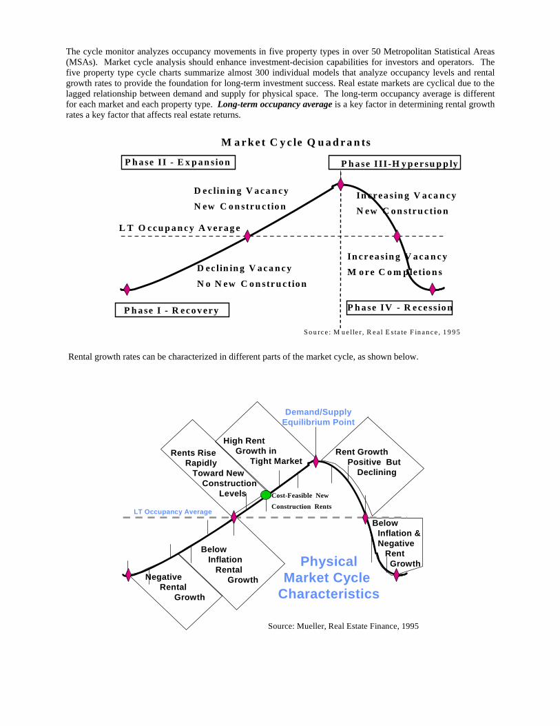
The cycle monitor analyzes occupancy movements in five property types in over 50 Metropolitan Statistical Areas (MSAs). Market cycle analysis should enhance investment-decision capabilities for investors and operators. The five property type cycle charts summarize almost 300 individual models that analyze occupancy levels and rental growth rates to provide the foundation for long-term investment success. Real estate markets are cyclical due to the lagged relationship between demand and supply for physical space. The long-term occupancy average is different for each market and each property type. Long-term occupancy average is a key factor in determining rental growth rates a key factor that affects real estate returns.

M a r k e t C y c le Q u a d r a n ts

L T O ccu p a n cy A v era g e

D ec lin in g V a ca n cy

N ew C o n stru c tio n

D ec lin in g V a ca n cy

N o N ew C o n stru c tio n

In crea s in g V a ca n cy

N ew C o n stru c tio n

In crea s in g V a ca n cy

M o re C o m p letio n s

P h a se II - E x p a n sio n

P h a se I - R eco v ery

P h a se III-H y p ersu p p ly

P h a se IV - R ecess io n

S o u rc e : M u e lle r , R e a l E s ta te F in a n c e , 1 9 9 5

Rental growth rates can be characterized in different parts of the market cycle, as shown below.

PhysicalMarket Cycle

CharacteristicsNegative

RentalGrowth

BelowInflation

RentalGrowth

Rents Rise Rapidly

Toward New Construction

Levels

High RentGrowth in

Tight Market

Demand/SupplyEquilibrium Point

Rent GrowthPositive But

Declining

-Below Inflation &Negative

RentGrowth

Cost-Feasible New Construction Rents

LT Occupancy Average

Source: Mueller, Real Estate Finance, 1995

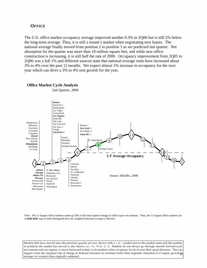
OFFICE The U.S. office market occupancy average improved another 0.3% in 2Q06 but is still 2% below the long-term average. Thus, it is still a tenant’s market when negotiating new leases. The national average finally moved from position 2 to position 3 as we predicted last quarter. Net absorption for the quarter was more than 18 million square feet, and while new office construction is increasing, it is still half the rate of 2000. Occupancy improvement from 2Q05 to 2Q06 was a full 1% and different sources state that national average rents have increased about 3% to 4% over the past 12 months. We expect almost 1% increase in occupancy for the next year which can drive a 3% to 4% rent growth for the year.

Orange County



11

1467

89

1012

13

115

1654321

Office Market Cycle Analysis2nd Quarter, 2006

AtlantaChicago

Dallas FWHouston

JacksonvilleKansas CityMilwaukee

Minneapolis

AlbuquerqueBaltimoreCincinnatiClevelandColumbus

Detroit New Orleans

NorfolkPhiladelphia

PittsburghSt. Louis

AustinMemphisPortlandRaleigh-Durham

W. Palm Beach

N. New JerseyOklahoma CityRichmondSan AntonioSeattleStamfordWilmington

CharlotteDenverEast BayFt. LauderdaleHonoluluOrlandoPhoenixRiverside+1Sacramento

BostonHartford+1Indianapolis Las VegasLong IslandLos AngelesNashvilleSalt Lake San FranciscoSan Jose+1TampaNATION+1

Miami+1New York+1San Diego+1Wash DC+1

Note: The 11-largest office markets make up 50% of the total square footage of office space we monitor. Thus, the 11-largest office markets are in bold italic type to help distinguish how the weighted national average is affected.

15

Markets that have moved since the previous quarter are now shown with a + or - symbol next to the market name and the number of positions the market has moved is also shown, i.e., +1, +2 or -1, -2. Markets do not always go through smooth forward-cycle movements and can regress, or move backward in their cycle position when occupancy levels reverse their usual direction. This can happen when the marginal rate of change in demand increases (or declines) faster than originally estimated or if supply growth is stronger (or weaker) than originally estimated.

Industrial

Industrial occupancy improved by 20 basis points in 2Q06, providing a 1.1% occupancy increase year over year from 2Q05. Eighteen cities improved their cycle position by at least one point, which moved the national average industrial cycle position to point #4 on the cycle graph. While new construction was strong at levels close to 2001, net absorption was almost 18 MSF for the quarter. Absorption continues to be strongest in southern California markets. Rents year over year were up 2.5% nationally. For the next year we expect another 0.5% occupancy increase which should drive rent growth in the 2.5% to 3% range.


11

1467

89

10 12

13

115

1654321

2nd Quarter, 2006


Industrial Market Cycle Analysis

DenverDetroit+1

HartfordHonolulu

Long Island+1MemphisStamford

Atlanta+1Baltimore+1 Cincinnati ColumbusIndianapolisJacksonville+1 Kansas City+1Milwaukee+1 MinneapolisNashvilleNew OrleansNew YorkNorfolkOklahoma CityOrlandoPortlandRaleigh-DurhamSan Francisco+2

BostonChicagoClevelandPhiladelphiaPittsburghSt. LouisTampa

Austin+1Charlotte+1

Dallas FW+1 East Bay

MiamiN. New Jersey+2

RichmondSacramento+1

San Jose+1San Antonio+1

Salt Lake+1Wash DC

NATION+1

Ft. Lauderdale PhoenixSan Diego+1Seattle

Las VegasLos AngelesOrange CountyW. Palm Beach+1

Riverside

Houston

Note: The 12-largest industrial markets make up 50% of the total square footage of industrial space we monitor. Thus, the 12-largest industrial markets are in bold italic type to help distinguish how the weighted national average is affected.

16

Markets that have moved since the previous quarter are shown with a + or - symbol next to the market name and the number of positions the market has moved is also shown, e.g., +1, +2 or -1, -2. Markets do not always go through smooth forward-cycle movements and can regress, or move backward in their cycle position when occupancy levels reverse their usual direction. This can happen when the marginal rate of change in demand increases (or declines) faster than originally estimated or if supply growth is stronger (or weaker) than originally estimated.

Apartment Apartment occupancy improved 10 basis points in 2Q06, this producing a 0.5% occupancy increase year over year. Multifamily construction starts were down 4% in the second quarter, 2% year over year and are hovering close to the long-term national average – which is sustainable. This shows moderation by the construction industry and reflects the decline in demand for condo conversions (the Condo craze is now over). Population growth and high housing costs still produce the best apartment markets. We anticipate occupancies to increase another 40 basis points in the next year. Rent growth was almost 3% year over year through the second quarter and we estimate 4% rent growth for the next year.

Norfolk


11

1467

89

10 12

115

1654321ColumbusDenverEast BayHonoluluN. New Jersey+2PhoenixSalt LakeSan Antonio+2Seattle+2NATION


Apartment Market Cycle Analysis2nd Quarter, 2006

BaltimoreSacramentoSan Francisco+2Cincinnati+1

ClevelandHartford+1HoustonIndianapolisLong Island+1MilwaukeeNew YorkPittsburghPortland+1RichmondStamford

13

ChicagoDetroit

MemphisMinneapolisNashville+2

New OrleansOklahoma City+1

PhiladelphiaRaleigh-Durham

St. Louis+2San Jose

Atlanta+1Austin

Boston+1Charlotte

Dallas FWKansas City+1

Wash DC

Jacksonvill1eLos Angeles

RiversideW Palm Beach

MiamiOrange County

San DiegoTampa

Ft. LauderdaleOrlandoLas Vegas

Note: The 10-largest multifamily markets make up 50% of the total square footage of multifamily space we monitor. Thus, the 10-largest multifamily markets are in bold italic type to help distinguish how the weighted national average is affected.

17


RETAIL Retail occupancy improved 0.2% in 2Q06 but is up only 0.5% year over year. Consumer spending is now reflecting higher gas prices as the recent detailed consumer spending report showed people are spending more on books and less on electronic media; more on beer-groceries and less on restaurants; more on toys/games but less on sporting equipment and jewelry; more on personal care and less on home care. Regional mall occupancy appears to have peaked as it is hard to increase occupancy past 95%. Thus, mall rental growth will be the best of the retail property types. The national retail average remains in the growth phase, at position 7 on the cycle where it appears to be stabilizing, even with a slowing economy. We expect the national occupancy position to hold at this level for the year, and rental growth to moderate to the 2%–3% range over the next year.


11

1467

89 12

13

115 1654321

Retail Market Cycle Analysis

10


2nd Quarter, 2006

BostonHoustonMilwaukeeNorfolkSt. LouisSacramentoSalt LakeSeattleNATION

DenverLos AngelesMinneapolisOrlandoPhiladelphiaPittsburghRichmondSan AntonioSan Jose

AustinJacksonville

Memphis

AtlantaCharlotte

Cleveland-1Dallas FW

HartfordIndianapolisKansas City

Oklahoma City

Baltimore-1MiamiOrange CountyPortland

Cincinnati+1ColumbusDetroitLas VegasNashvilleN. New JerseyRaleigh-DurhamRiversideStamfordW. Palm Beach

ChicagoEast BayHonoluluSan FranciscoTampaWash DC

New Orleans

Ft. LauderdaleLong IslandNew YorkSan Diego

Phoenix

Note: The 15-largest retail markets make up 50% of the total square footage of retail space we monitor. Thus, the 15-largest retail markets are in bold italic type to help distinguish how the weighted national average is affected.

18


HOTEL Hotel occupancies improved 0.3% in 2Q06 and 1.2% year over year. Demand continues to be strong across the board with air travel up and most planes full. It is good news for the hotel industry that airlines have been able to become profitable in the face of higher fuel prices, but at the expense of few flight options for travelers. Construction starts have been very strong in many markets with Lodging Econometrics (www.lodging-econometrics.com) reporting a 50% year-over-year increase, which is a new high for this cycle, but about 15% below the peak set in 1998. Construction is highest in Washington, New York, Dallas, Los Angeles and Atlanta. Occupancy levels are now expected to improve another 1% over the next year, which would provide a RevPAR growth more than 10% in the next year as well.


1467

89 12

13

115

165

4321

1110


Hotel Market Cycle Analysis2nd Quarter, 2006

BostonCincinnati

DetroitIndianapolis

Pittsburgh

HartfordN. New Jersey+1PortlandRichmond+1Salt Lake-1 San Jose-1

Charlotte-1DallasLong IslandLas Vegas+1Milwaukee+1Minneapolis+1Nashville+1 MiamiRaleigh-Durham+1San Antonio-1San FranciscoStamford+2Tampa

ClevelandColumbus

Kansas CitySt. Louis

AtlantaBaltimore+2Ft. Lauderdale+1JacksonvilleNorfolkOrlandoPhiladelphiaRiverside+1SacramentoNATION

Chicago+1East Bay

DenverHoustonMemphis

New Orleans Oklahoma City

Seattle-1AustinLos Angeles Orange CountyPhoenixSan DiegoWash DCW. Palm Beach

HonoluluNew York+1

Note: The 14-largest hotel markets make up 50% of the total square footage of hotel space that we monitor. Thus, the 14-largest hotel markets are in boldface italics to help distinguish how the weighted national average is affected.

19


http://www.lodging-econometrics.com/

http://www.lodging-econometrics.com/

20

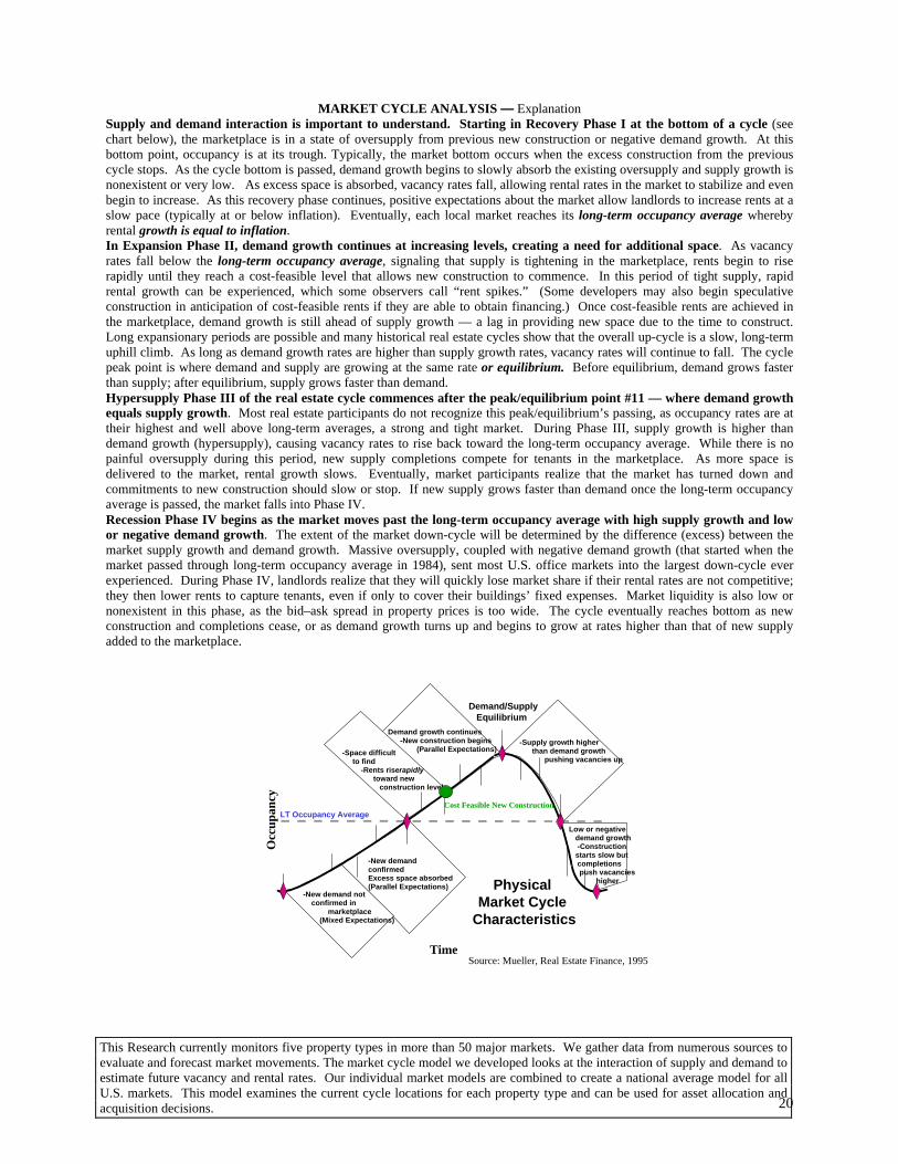
MARKET CYCLE ANALYSIS — Explanation

Supply and demand interaction is important to understand. Starting in Recovery Phase I at the bottom of a cycle (see chart below), the marketplace is in a state of oversupply from previous new construction or negative demand growth. At this bottom point, occupancy is at its trough. Typically, the market bottom occurs when the excess construction from the previous cycle stops. As the cycle bottom is passed, demand growth begins to slowly absorb the existing oversupply and supply growth is nonexistent or very low. As excess space is absorbed, vacancy rates fall, allowing rental rates in the market to stabilize and even begin to increase. As this recovery phase continues, positive expectations about the market allow landlords to increase rents at a slow pace (typically at or below inflation). Eventually, each local market reaches its long-term occupancy average whereby rental growth is equal to inflation. In Expansion Phase II, demand growth continues at increasing levels, creating a need for additional space. As vacancy rates fall below the long-term occupancy average, signaling that supply is tightening in the marketplace, rents begin to rise rapidly until they reach a cost-feasible level that allows new construction to commence. In this period of tight supply, rapid rental growth can be experienced, which some observers call “rent spikes.” (Some developers may also begin speculative construction in anticipation of cost-feasible rents if they are able to obtain financing.) Once cost-feasible rents are achieved in the marketplace, demand growth is still ahead of supply growth — a lag in providing new space due to the time to construct. Long expansionary periods are possible and many historical real estate cycles show that the overall up-cycle is a slow, long-term uphill climb. As long as demand growth rates are higher than supply growth rates, vacancy rates will continue to fall. The cycle peak point is where demand and supply are growing at the same rate or equilibrium. Before equilibrium, demand grows faster than supply; after equilibrium, supply grows faster than demand. Hypersupply Phase III of the real estate cycle commences after the peak/equilibrium point #11 — where demand growth equals supply growth. Most real estate participants do not recognize this peak/equilibrium’s passing, as occupancy rates are at their highest and well above long-term averages, a strong and tight market. During Phase III, supply growth is higher than demand growth (hypersupply), causing vacancy rates to rise back toward the long-term occupancy average. While there is no painful oversupply during this period, new supply completions compete for tenants in the marketplace. As more space is delivered to the market, rental growth slows. Eventually, market participants realize that the market has turned down and commitments to new construction should slow or stop. If new supply grows faster than demand once the long-term occupancy average is passed, the market falls into Phase IV. Recession Phase IV begins as the market moves past the long-term occupancy average with high supply growth and low or negative demand growth. The extent of the market down-cycle will be determined by the difference (excess) between the market supply growth and demand growth. Massive oversupply, coupled with negative demand growth (that started when the market passed through long-term occupancy average in 1984), sent most U.S. office markets into the largest down-cycle ever experienced. During Phase IV, landlords realize that they will quickly lose market share if their rental rates are not competitive; they then lower rents to capture tenants, even if only to cover their buildings’ fixed expenses. Market liquidity is also low or nonexistent in this phase, as the bid–ask spread in property prices is too wide. The cycle eventually reaches bottom as new construction and completions cease, or as demand growth turns up and begins to grow at rates higher than that of new supply added to the marketplace.

Physical Market Cycle

Characteristics

-New demand not confirmed in marketplace (Mixed Expectations)

-New demandconfirmedExcess space absorbed(Parallel Expectations)

-Space difficult to find -Rents rise rapidly toward new construction levels

-Demand growth continues -New construction begins (Parallel Expectations)

Demand/Supply Equilibrium

-Supply growth higher than demand growth pushing vacancies up

-Low or negative demand growth -Construction starts slow but completions push vacancies higher

Cost Feasible New ConstructionLT Occupancy Average

Occ

upan

cy

TimeSource: Mueller, Real Estate Finance, 1995

This Research currently monitors five property types in more than 50 major markets. We gather data from numerous sources to evaluate and forecast market movements. The market cycle model we developed looks at the interaction of supply and demand to estimate future vacancy and rental rates. Our individual market models are combined to create a national average model for all U.S. markets. This model examines the current cycle locations for each property type and can be used for asset allocation and acquisition decisions.

21

Important Disclosures and Certifications I, Glenn R. Mueller, Ph.D. certify that the opinions and forecasts expressed in this research report accurately reflect my personal views about the subjects discussed herein; and I, Glenn R. Mueller, certify that no part of my compensation from any source was, is, or will be directly or indirectly related to the content of this research report.

The information contained this report: (i) has been prepared or received from sources believed to be reliable but is not guaranteed; (ii) is not a complete summary or statement of all available data; (iii) is not an offer or recommendation to buy or sell any particular securities; and (iv) is not an offer to buy or sell any securities in the markets or sectors discussed in the report. The opinions and forecasts expressed in this report are subject to change without notice and do not take into account the particular investment objectives, financial situation or needs of individual investors. Any opinions or forecasts in this report are not guarantees of how markets, sectors or individual securities or issuers will perform in the future, and the actual future performance of such markets, sectors or individual securities or issuers may differ. Further, any forecasts in this report have not been based on information received directly from issuers of securities in the sectors or markets discussed in the report. Dr. Mueller serves as a Real Estate Investment Strategist with Dividend Capital Group. In this role, he provides investment advice to Dividend Capital Group and its affiliates regarding the real estate market and the various sectors within that market. Mr. Mueller’s compensation from Dividend Capital Group and its affiliates is not based on the performance of any investment advisory client of Dividend Capital Group or its affiliates. Dividend Capital Group is a real estate investment management company that focuses on creating institutional-quality real estate financial products for individual and institutional investors. Dividend Capital Group and its affiliates also provide investment management services and advice to various investment companies, real estate investment trusts, and other advisory clients about the real estate markets and sectors, including specific securities within these markets and sectors. Investment advisory clients of Dividend Capital Group or its affiliates may from time to time invest a significant portion of their assets in the securities of companies primarily engaged in the real estate industry, such as real estate investment trusts, or in real estate itself, and may have investment strategies that focus on specific real estate markets, sectors and regions. Real estate investments purchased or sold based on the information in this research report could indirectly benefit these clients by increasing the value of their portfolio holdings, which in turn would increase the amount of advisory fees that these clients pay to Dividend Capital Group or its affiliates. Dividend Capital Group and its affiliates (including their respective officers, directors and employees) may at times: (i) release written or oral commentary, technical analysis or trading strategies that differ from or contradict the opinions and forecasts expressed in this report; (ii) invest for their own accounts in a manner contrary to or different from the opinions and forecasts expressed in this report; and (iii) have long or short positions in securities or in options or other derivative instruments based thereon. Furthermore, Dividend Capital Group and its affiliates may make recommendations to, or effect transactions on behalf of, their advisory clients in a manner contrary to or different from the opinions and forecasts in this report. Real estate investments purchased or sold based on the information in this report could indirectly benefit Dividend Capital Group, its affiliates, or their respective officers, employees and directors by increasing the value of their proprietary or personal portfolio holdings. Dr. Mueller may from time to time have personal investments in real estate, in securities of issuers in the markets or sectors discussed in this report, or in investment companies or other investment vehicles that invest in real estate and the real estate securities markets (including investment companies and other investment vehicles for which Dividend Capital Group or an affiliate serves as investment adviser). Real estate investments purchased or sold based on the information in this report could directly benefit Dr. Mueller by increasing the value of his personal investments.

© 2006 Dividend Capital Group, 518 17th Street, Denver, CO 80202

22

APPENDIX B Literature Review Real estate cycles were first discussed by Homer Hoyt in 1933 in his analysis of the Chicago marketplace. Since that time market cycles have received scattered attention over the years. Pritchett (1984) theorized that there is a national real estate market cycle, but the cycles for each property type were not coincident. He stated that supply growth and decline always lagged demand growth and decline, thus turning points in the top and bottom of any cycle could be determined when the supply growth and demand growth were moving in opposite directions. However, recognition of turning points was less useful to investors than anticipation of such points. He applied these ideas by stating that the most advantageous buying opportunities generally exist during late declining, bottom, and early rising portions of the real estate market cycle. Witten (1987) stated that every city had its own property cycles which were unique in length (time) and degree of change (magnitude) and were dependent on the internal dynamics of each market. He also stated that new supply while being cyclical is somewhat more volatile than demand, since supply is often determined by the availability of financing rather than by market need. He also observed that markets seldom move as smoothly as the classically drawn curves, but instead move in "fits and starts" causing investors to hesitate and wait for clear signs as to market changes. Brown (1984) described cycle modeling as a simplification of the complexities of reality which hopefully capture the crucial features of the economic sector or system being studied. He believed that time series should be used to determine the length and magnitude of cycles as it seeks to measure movement over time. Also the longer the length of time studied, the better the understanding of the cycle movement. A key to cycle research is the identification and removal of trend and seasonal components inherent in time series data. He concluded that if feasibility analysts, investment advisors, and principals or lenders are to give credibility to market cycle analysis, much more research needs to be done. There are currently no uniform measurement procedures available, making it difficult to agree on the length and magnitude of cycle movements. He concluded that the downside of market cycles creates extreme economic obsolescence, thus real estate professionals need to maintain the perspective of cyclical timing in their decision making. Wheaton (1987) using a sample of 10 cities, estimated the national office market cycle to have a length of between 10 and 12 years. He found that each city had a turning point (peak or trough) in its own market cycle that was within one or two years of the combined average of the 10 cities. He studied the causes of market movement that made the office market cyclical. One of his findings was that the tenure structure of office leases was usually long-term (e.g. 10-15 years). His explanatory model found that expected employment growth was significant in determining cycle behavior thus creating an adaptive demand model (supply will react to increased demand with a lag) and concluded that supply responds more readily to the state of the economy (as developers adjust their expectations to general economic indicators such as GDP growth and interest rates) than to actual local demand. This adjustment can actually help curtail the magnitude of a cycle as GDP growth is more moderate than local demand growth. He concluded that both supply and demand respond to changes in the economy although supply is more responsive than demand. Wheaton & Torto (1988) studied rent and vacancy rate cycles and found that there was a market rental adjustment mechanism that caused real office rents to drop approximately 2% annually for every percentage point of excess vacancy above the long-term average in the market. They also found that the average office vacancy rate was trending upward over the 1968 to 1986 time period studied. Probably due to the excessively high supply rates of the 1980s. Pyhrr, Webb, and Born (1990a, 1990b) in two different articles compare typical trend models for real estate analysis with a theoretical cycle model based upon demand, supply and inflation inputs. They conclude that the timing of acquisition and disposition in the cycle can be very important to the overall return received from real estate investments. Pyhrr, Born, Robinson and Lucas (1996) compare traditional valuation methods against a model using cyclical assumptions including demand, supply, absorption, occupancy rates and rental rate differences between newly constructed and existing properties. They conclude that valuations with cyclical assumptions can dramatically alter valuation conclusions, but that a cyclical model may be a better indicator of investment value (long-term), than market value (one point in time). Mueller and Laposa (1994 and 1995) discussed the difference between overall market and submarket cycles. Their research found that submarkets can move differently from the overall market cycle in the short run, but submarkets will typically trend with overall market movements in the long run, because the locational advantages of a submarket become appropriately priced in the marketplace over time.

23

Mueller (1995) stratified real estate market cycles into two distinct cycle types: first, a physical cycle that described only the demand, supply, and occupancy of physical space in a local market that affects rental growth and second, a financial cycle that examined the capital flows into real estate for both existing properties and new construction which affects property prices. This separation between physical and financial cycles helps to clarify earlier work that mixed many definitions and helps explain the lag that appears to exist between market occupancy and rental movements versus real estate prices. Grenadier (1995) developed a theoretical option pricing model of how vacancy rates and rental rates interact. He hypothesized that there is considerable inertia from existing building owners to adjust rents and occupancy levels in reaction to changing economic environments (the owner’s option to rent). He also attempted to explain the recurrence of overbuilding during periods of low occupancy, by proposing that the costs of re-leasing can make vacancy “sticky”, because landlords may choose to wait for higher rental rates before leasing space and that long construction times coupled with the inability to reverse a construction start decision can cause too much new supply. He also modeled demand volatility and theorized that markets with greater demand volatility had a higher propensity to overbuild. The economic literature addresses price dispersion under various search models. Butters (1977) postulated that a consumer’s imperfect information is insufficient to support price dispersion. Others have shown that heterogeneity among producers explains price dispersion [Carlson and McAfee (1983), MacMinn (1980)]. Nitzan and Tzur (1991) show that price dispersion can exist even when fully rational economic agents on both sides are homogeneous. Fershyman and Fishman (1992) present a dynamic search model which accounts for cyclical patterns of prices and demand. Thus, the behavior, strategies, and expectations of landlords and search behavior of tenants at various points in the real estate cycle may be explained by search theory models and price dispersion theory when we examine the rent price distributions in real estate markets. Applications to real estate value pricing are more difficult as homogeneous expectations are difficult to apply to heterogeneous assets.

Bibliography Born, Waldo L, and Pyhrr, Steven A., “Real Estate Valuation, The Effect of Market and Property Cycles”, Journal of Real Estate Research, 9(4), 1994 Brown, Gordon T., "Real Estate Cycles Alter the Valuation Perspective," Appraisal Journal, 52(4): 539-549, 1984. Butters, G. R. “Equilibrium Distribution of Sales and Advertising Prices,” Review of Economic Studies 44 (1977) 487-491. Carlson, J.A. and McAfee, R.D., “Discrete Equilibrium Price Dispersion,” Journal of Political Economy (1983) 91, 480-493 Fershtman, Chaim and Fishman, Arthur, “Price Cycles and Booms: Dynamic Search Equilibrium”, The American Economic Review (1992) Vol 82, No. 5, 1221-1233. Gilberto, Michael S., “A Note on Commercial Mortgage Flows and Construction”, Journal of Real Estate Research, 7(4) 1992, pp. 485-492. Grenadier, Steven H., “The Persistence of Real Estate Cycles” Journal of Real Estate Finance and Economics, (1995) 10:95-119 Hosier, Amy L. W. “A New Look at Rental-Price Adjustment in Office Markets: Do Vacancy Rates Really Matter?”, Real Estate Research Institute. MacMinn, R. D. “Search and Market Equilibrium,” Journal of Political Economy (1980) 88, 308-315. Mueller, Glenn R., “Understanding Real Estate’s Physical and Financial Market Cycles”, Real Estate Finance, Spring 1995 12, 1 pp47-52. Mueller, Glenn R., Laposa Steven P., Real Estate Market Evaluation Using Cycle Analysis, paper presented at the 1995 International Real Estate Society Conference, Stockholm, Sweden.

24

Mueller, Glenn R., Laposa Steven P., Evaluating Real Estate Markets Using Cycle Analysis, paper presented at the 1994 American Real Estate Society Meetings in Santa Barbara, CA. Mueller, Glenn R., Laposa Steven P., Submarket Cycle Analysis- A Case study of submarkets in Philadelphia, Seattle and Salt Lake, paper presented at the 1994 American Real Estate Society Meetings in Santa Barbara, CA. Nitzan, Shmuel, and Tzur, Joseph, “Costly Diagnosis and Price Dispersion” Economics Letters 36 (1991) 245-251. Pritchett, Clayton P., "Forecasting the Impact of Real Estate Cycles on Investments," Real Estate Review, 13(4): 85-89, 1984. Pyhrr, Steven A., Born, Waldo L., Webb, James R., “Development of a Dynamic Investment Strategy Under Alternative Inflation Cycle Scenarios”, Journal of Real Estate Research, 5(2), 1990 pp177-193. Pyhrr, Steven A., Webb, James R Born, Waldo L.,, “Analyzing Real Estate Asset Performance During Periods of Market Disequilibrium, Under Cyclical Economic Conditions”, Research in Real Estate, JAI Press, Vol.3, 1990. Pyhrr, Steven A., Born, Waldo L., Robinson T., and Lucas J., “Valuation in a Changing Economic and Market Cycle”, Appraisal Journal, Fall, 1996 Smith, Stanley D., Woodward, Larry R., Schulman, Craig T., “The effect of the Tax Reform Act of 1986 & Overbuilt Markets on Commercial Office Property Values.” Journal of Real Estate Research, 19(3), 2000 pp 301-320 Wheaton, William C., "The Cyclic Behavior of the National Office Market," AREUEA Journal 15(4): 281-299, 1987. Wheaton, William C. and R. G. Torto, "Vacancy Rates and the Future of Office Rents," AREUEA Journal 16(4): 430-455, 1988. Wheaton, William C., Torto, Raymond G., Southard, Jon A. “Flight To or From Quality” paper presented at the 1995 ARES meeting Witten, Ronald G., "Riding the Real Estate Cycle," Real Estate Today, 42-48, August 1987.

Documents

What Will the Next Real Estate Cycle Look Like · in the same cycle and that the residential real estate market and commercial real estate market are closely ... New commercial properties