Embed Size (px)
Citation preview
What You See is Not What You Get:The Costs of Trading Market Anomalies
Andrew J. Patton and Brian M. Weller⇤
Duke University
March 9, 2018
Abstract
Is there a gap between the profitability of a trading strategy “on paper” and thatwhich is achieved in practice? We answer this question by developing two new techniquesto measure the real-world implementation costs of financial market anomalies. The firstmethod extends Fama-MacBeth regressions to compare the on-paper returns to factorexposures with those achieved by mutual funds. The second method estimates averagereturn differences between stocks and mutual funds matched on risk characteristics.Unlike existing approaches, these techniques deliver estimates of implementation costswithout estimating parametric microstructure models from trading data or explicitlyspecifying factor trading strategies. After accounting for implementation costs, typicalmutual funds earn low returns to value and no returns to momentum.
JEL: G12, G14, G23Keywords: Trading Costs, Performance Evaluation, Mutual Funds, Market Efficiency
⇤Email: [email protected], [email protected]. We thank Alex Chinco, Andrew Detzel, Campbell Har-vey, David Hsieh, Robert Korajczyk, Alex Kostakis, Juhani Linnainmaa, Toby Moskowitz, and seminar participantsat the Yale Junior Finance Conference, Duke Fuqua, Manchester, the UBC Winter Finance Conference, and JohnCochrane’s 60th Birthday Conference for valuable comments and discussion.

I. Introduction
Empirical asset pricing overflows with explanations for differences in average returns acrosssecurities. The proliferation of predictors distracts from bona fide market anomalies from which wemight draw lessons about risks, preferences, and beliefs. Increasing computing power acceleratesthe rate of factor discovery and the urgency of separating empirical regularities from journal-friendly fictions. Recent calls to action by Harvey, Liu, and Zhu (2016), Harvey (2017), and Hou,Xue, and Zhang (2017) have focused on high false discovery rates and scurrilous academic practices.Fundamentally they question whether candidate factors are real, statistical accidents, or intentionaldeceptions.
We give on-paper trading strategies the benefit of the doubt and instead question whether theseare actionable in practice, thereby representing true expected return factors or market anomalies.This line of inquiry originates with Fama (1970), who considers the role of transactions costs indefining market efficiency and departures therefrom. Despite nearly fifty years of subsequent re-search, accurately measuring real-world transactions costs for academic factors remains a formidablechallenge. Existing approaches generally fall into two categories. The first category entails usingproprietary trading data to analyze the transactions costs for a single firm (e.g., Keim and Mad-havan (1997), Engle, Ferstenberg, and Russell (2012), and Frazzini, Israel, and Moskowitz (2015)).Although selected firms are almost by definition not representative of asset managers as a whole,such analyses provide an informative lower bound on the transactions costs of factor strategies. Thesecond approach uses market-wide trading data such as NYSE Trade and Quote (TAQ) to estimateprice impact functions for individual securities. These papers then accumulate simulated costs oftrades implied by dynamic factor strategies (e.g., Lesmond, Schill, and Zhou (2004), Korajczyk andSadka (2004), and Novy-Marx and Velikov (2016)). Papers in this camp either establish a lowerbound on trading costs by dispensing with non-proportional costs of trade or estimate parametricprice impact models and extrapolate trading costs beyond small portfolio sizes.
We introduce two new methodologies for measuring real-world implementation costs for fac-tor trading strategies. Our approaches differ from existing methods in that they do not utilizespecialized trading data or parameteric transaction cost models, nor do they require the user totake a stand on the exact form of factor trading strategies. This latter feature is particularly im-portant because high-turnover academic factors like momentum may have industry variants withsignificantly lower implementation costs. Together these features facilitate the estimation of theall-in implementation costs for several academic factors and a representative population of assetmanagers.
Our first approach is an extension of the familiar Fama and MacBeth (1973) procedure. Fama-MacBeth regressions estimate factor loadings �ik with time-series regressions for each test asseti and each factor k, and then estimate the compensation per unit of factor exposure �kt usingcross-sectional regressions at each date t. Standard test assets are based on stock portfolios, and
1

the resulting estimates of of factor exposure compensation, denoted �Skt, represent the “on-paper”
profitability of a given factor strategy. We augment the set of test assets to include all the set of all7,331 U.S. domestic mutual funds, and we allow the compensation earned by mutual funds for thesame exposure to a given factor �MF
kt to differ from that which is available on paper. Unlike stockportfolio returns, (gross) mutual fund returns reflect the real-world implementation costs of factorstrategies, thus the difference between mutual fund and stock portfolio compensation delivers anestimate of implementation costs for factor k.1,2 Because costs per unit of exposure are likely tobe negatively correlated with factor exposures—funds that earn greater net returns to a factor aremore likely to take greater exposures to it—our estimate of implementation costs represents a lowerbound on the costs faced by a representative mutual fund.
The Fama-MacBeth approach described above compares slopes or incremental compensation forrisk for stocks and mutual funds. Our second approach directly compares levels of compensationfor stocks and mutual funds with similar risk characteristics. To make this comparison, we sortstocks into quintile portfolios based on characteristics, as in portfolio sorts or “high minus low”factor construction. Then, for each stock in quintile q at date t, we construct a matched sampleof mutual funds consisting of the three nearest mutual funds as assessed by Mahalanobis distanceon factor betas.3 The difference in returns between stocks and matched mutual funds �q
kt is ourmatched pairs estimate of implementation costs associated with real-world trading in beta-quintileq of factor k at date t. Because implementation costs are likely to be significantly higher on theshort side of factor strategies, the difference in long-only returns �5
kt delivers a lower bound onthe implementation costs of a 5–1 long-short strategy for factor k. This analysis has the ancillarybenefit of controlling for differences in the distribution of betas between stock portfolios and mutualfunds, which may be important if high compensation for factor exposure is earned only in somesegments of this distribution.
Our empirical analysis focuses on the implementation costs of mutual funds for the market(MKT ),4 value (HML), size (SMB), and momentum (UMD). We choose these factors becausethey comprise the dominant empirical models in academic finance (e.g., Fama and French (1992)and Carhart (1997)), and they serve as the basis for guiding hundreds of billions of dollars inquantitatively managed investments. We study mutual funds as our set of asset managers becausethey collectively manage more than $16 trillion of capital in the United States,5 and the mutual fund
1We use gross returns to focus on the efficiency of mutual funds’ investing technology rather than on the distributionof rents between managers and investors embedded in net returns.
2Our more sophisticated approaches account for time- and cross-sectional variation in implementation costs, whichwe discuss further below.
3Betas for stocks and matched mutual funds do not perfectly coincide. We follow Abadie and Imbens (2006, 2011)to shift mutual fund returns by the compensation for a “local” difference in betas. Because this return-adjustmenttakes the form of a cross-sectional regression of returns on betas, our approach marries matched pairs techniques withtraditional factor models.
4We use the CRSP value-weighted market portfolio net of the one-month Treasury bill rate as our zero-cost marketfactor proxy.
5Source: the 2017 Investment Company Fact Book, available at http://www.icifactbook.org/.
2
industry has been better populated for a longer period of time than alternative asset managers suchas hedge funds. Our approaches are readily extended to other factors and other market participants,however.
Our analysis delivers three new empirical facts on the implementation costs of anomalies fortypical mutual funds. First, momentum strategies suffer extreme underperformance in practice:our estimates of annual implementation costs are in the range of 2.2%–8.3%, which eliminates mostprofits accruing to momentum during the 1970–2016 period.6 We conclude—as Lesmond, Schill,and Zhou (2004) do—that momentum strategies are unprofitable for typical asset managers. Sec-ond, mutual fund implementation costs sharply reduce returns to the value factor, although ourapproaches differ on the extent of underperformance; the corresponding average annual differencesbetween on-paper and mutual fund performance for value are 2.4%–5.3%.7 By contrast, mutualfunds implement market and size factor exposure relatively well compared to the academic bench-mark, although they still underperform in capturing outsize returns to the small-size characteristic.Third, average implementation costs are stationary despite secular declines in bid-ask spreads andcommissions since 1970. Industry inflows increase transactions costs, which neutralize reductionsin costs to the first dollar traded in factor strategies. This channel provides a non-proportionalcosts of trading rationale for Pastor and Stambaugh (2012)’s industry-level diseconomies of scalein asset management.
As a second empirical contribution, we focus on cross-sectional heterogeneity in implementa-tion costs and demonstrate the importance of benchmarking performance and considering marketefficiency as a function of investors’ trading technology. While the typical firm’s compensation formomentum is indistinguishable from zero, subsets of the mutual fund universe may achieve positivereturns to momentum net of costs. A focused analysis on smaller market segments is importantfrom an aggregate market efficiency perspective because a violation exists if the marginal investorsees anomalous profits, even if a typical investor does not. For this purpose we segment the mutual-fund universe by (lagged) total net assets. Size is a natural sorting dimension because Berk andGreen (2004), Pastor, Stambaugh, and Taylor (2015), Berk and van Binsbergen (2015), and otherslink scale to gross-of-fees performance. We rerun our cross-sectional analysis using each mutualfund size category separately, and we confirm that small and large mutual funds achieve differ-ent returns to momentum from “typical” mutual funds. Using this insight we reconcile conflictingevidence on the transactions-cost rationale for the continued existence of the momentum anomaly.
While our new approaches deliver simple, nonparametric, estimates of the implementation costsfor factor trading strategies, they do face some limitations. Firstly, as mentioned above, bothapproaches deliver lower bounds on implementation costs. In our empirical analysis these bounds
6The estimated implementation gap is even larger among the set of mutual funds with strictly positive momentumbetas.
7These results are robust to the exclusion of microcap stocks. Microcap stocks explain at most 17%–27% of themeasured implementation gap.
3
do not greatly limit the conclusions we can draw: the estimated costs are already so high as toeliminate or severely attenuate the on-paper profitability of strategies like value and momentum fortypical mutual funds. For other strategies, estimates that indicate positive returns net of costs donot necessarily imply that an anomaly can be implemented by typical investors. In this sense ourmeasures can diagnose an implementation problem with a factor, but they cannot deliver a cleanbill of health.
Secondly, our techniques rely on real-world asset managers to reveal implementation coststhrough realized returns to their chosen factor exposures. We require a subset of asset managersto invest in the factor of interest over an extended period of time. This requirement is not likely tobe satisfied when studying a factor that is new to the academic literature and fund managers havenot had an opportunity to trade on this factor.8
Finally, like much of the literature on performance evaluation, our methods are susceptible tocriticism of the choice of factors included in the analysis. A manager who is following a strategythat does not correspond to an approximate linear combination of those included in the model mayappear to have high implementation costs for the included strategies, even though she has low costsfor the strategy actually being implemented. In our application we verify that omitted mutual fundstrategies do not drive our high implementation cost estimates by replicating performance gaps forfunds with returns almost completely explained by the academic factors (the average R2 of thefour-factor model for these funds’ return histories is 95%). For these funds, the scope for omittedstrategies is too small to explain the observed real-world performance gaps. In general settings,however, our methods speak only to implementation costs of the projection of the returns to tradedstrategies on the included factors.
Confronted with hundreds of cross-sectional return predictors, recent papers have proposedtechniques to help focus attention on the most robust anomalies.9 Notwithstanding the limitationsof our approach mentioned above, we recommend our methodologies as complements to thesesuggestions for three reasons. First, our methodologies provide an easy test of the real-worldapplicability of a conjectured factor. If mutual funds are not compensated for factor exposure,a factor is less likely to be real or implementable. We anticipate that our implementability testgeneralizes Hou, Xue, and Zhang (2017)’s suggestion to exclude microcap stocks in that strategiesrelying on the smallest stocks would see large real-world performance attrition relative to paperportfolios. Second, our approaches provide orthogonal information to existing asset pricing tests.While it might be possible to reconfigure empirical choices to elevate a t-statistic from 2 to 3,we view it as less likely that an entirely new hurdle can be cleared for spurious factors. Third,
8This caveat does not apply in the particular case of momentum. Grinblatt, Titman, and Wermers (1995) arguethat momentum-like strategies are endemic among mutual funds in their 1975–1984 sample, decades before thepublication of Jegadeesh and Titman (1993).
9Harvey, Liu, and Zhu (2016) advocate raising statistical significance thresholds. Harvey (2017) endorses mixingstandard thresholds with Bayesian priors on the plausibility of a factor. Giglio and Xiu (2017) suggest “cleaning”factors of noise using variation in test asset returns.
4
the computational burden of our technique is low, and mutual fund performance data is readilyavailable to empirical researchers. With our techniques the barriers to entry for cross-sectionalasset pricing work are not appreciably raised.
II. Related Literature
The Fama and French three-factor model has been the benchmark for empirical asset pricingsince its introduction in 1992. This empirical model supplanted the CAPM, but its new valueand size factors had little theoretical motivation.10 As factors continued to emerge over the nextquarter century—most notably, the momentum anomaly of Jegadeesh and Titman (1993)—severalstrands of literature emerged in an attempt to tame the “factor zoo” (Cochrane (2011)). Oneactive strand investigates the implementation costs of anomalies with a particular focus on size,value, and momentum anomalies. While transactions costs cannot explain why expected returndiscrepancies come to be in the first place, this literature (reviewed below) seeks to rationalize thecontinued existence of market anomalies as their byproduct. Our paper advances this line of inquiryby introducing a new and readily generalizable approach for measuring the real-world transactionscosts of return factors and anomalies.
Existing methods for measuring implementation costs take two approaches. The first approachuses specialized trading data to evaluate the costs of trade for large investment managers withthe implicit assumption that these managers are representative of sophisticated investment man-agers. These papers typically assess trading costs using Perold (1988)’s implementation shortfallmeasure, which captures the difference between realized profits and on-paper profits using a presetdecision price. This approach dates back at least to Keim and Madhavan (1997), who analyzethe transactions costs of a variety of investment styles for $83 billion of trades.11 A key challengeto this method is that institutional trading is endogenous; traders are particularly aggressive intheir trading targets when liquidity is readily available, which in turn imparts a downward biasto estimated cost functions. Frazzini, Israel, and Moskowitz (2015) overcome this challenge byusing data from an investment manager whose trading targets are model-generated and selectedirrespective of market conditions. Armed with more than $1 trillion of trades, they analyze value,size, and momentum anomalies and find that all of them are implementable and scalable to tensor hundreds of billions of dollars of invested capital. By their reckoning, major anomalies continueto be anomalous if their asset manager’s costs are representative of typical investment managers’costs.
The second approach trades off accuracy for representativeness in estimating transactions costs.
10Banz (1981) and Basu (1977) document price-earnings ratios and market capitalization as characteristics associ-ated with deviations from the CAPM.
11Other studies use Keim and Madhavan (1997)’s calibrated transaction cost functions to decompose fund per-formance for a larger universe of funds. For example, Wermers (2000), like our study, finds that transactions costsmeaningfully erode mutual fund returns.
5

Rather than using proprietary trading data for a single asset manager to estimate costs directly,other studies derive transactions costs using aggregate price and transaction records and extrapolateestimated price impact functions to factor trading strategies.12 Much of this literature focuses onthe momentum anomaly because of its high turnover, and even the originating article establishingthe momentum anomaly considers a trading-costs explanation (Jegadeesh and Titman (1993) andlater Jegadeesh and Titman (2001)). Notably none of these papers use precise “all in” tradingcost measures like implementation shortfall because theoretical or “decision-date” prices are notobtainable outside of specialized trading data.
Chen, Stanzl, and Watanabe (2002) estimate separate price impact functions for 5,173 individualstocks and calculate the trading costs accruing to size, value, and momentum strategies. Theauthors suggest that all factors have break-even carrying capacities on the order of millions of dollars(HML) to hundreds of millions of dollars (SMB). By their calculations, factor strategies are notinvestable. Lesmond, Schill, and Zhou (2004) suggest that momentum trades in “disproportionatelyhigh cost securities” rather than the typical-transactions cost securities Jegadeesh and Titman(1993) use for approximating the costs of trading momentum. Using effective spreads from TAQ,commission schedules from a discount brokerage, and “all-in” frictions implied by zero-trading days(Lesmond, Ogden, and Trzcinka (1999)), Lesmond, Schill, and Zhou (2004) argue that trading costserase the returns to the momentum anomaly.
Korajczyk and Sadka (2004) present more optimistic results on the investability of factor strate-gies. Korajczyk and Sadka (2004) estimate effective and quoted spreads and non-proportionaltrading costs functions of Glosten and Harris (1988) and Breen, Hodrick, and Korajczyk (2002)using TAQ data. In utilizing different non-proportional cost functions from Lesmond, Schill, andZhou (2004), Korajczyk and Sadka (2004) extrapolate trade-level costs to find positive net-of-cost returns to the momentum anomaly. They invert their cost function estimates to obtain abreak-even momentum strategy carrying capacity of $5 billion. While much smaller than Frazz-ini, Israel, and Moskowitz (2015)’s estimates, these carrying capacities are also measured basedon older data for which transactions costs are significantly higher (Lou and Sadka (2016)). Novy-Marx and Velikov (2016) follows a similar approach, but they focus only on proportional costs toestablish a lower bound. The authors measure trading costs using effective spreads recovered fromHasbrouck (2009)’s Bayesian Gibbs sampler and tally costs of trading size, value, and momentumstrategies, among others. Although the paper focuses on performance evaluation, Novy-Marx andVelikov (2016) find a momentum strategy carrying capacity of $5 billion (as in Korajczyk and Sadka(2004)), and they find size and value carrying capacities of $170 billion and $50 billion respectively(which are comparable to Frazzini, Israel, and Moskowitz (2015)’s estimates).
Our work complements the two existing approaches to measuring implementation costs withnew cross-sectional techniques that combine the best elements of both. Like papers that utilize
12Grundy and Martin (2001) and Barroso and Santa-Clara (2015) invert this logic and calculate the transactionscosts that would be required to wipe out the momentum anomaly.
6

proprietary trading data, our estimates reflect the all-in costs of implementing factor strategies,and they apply equally well for past and modern market environments (for which Lesmond, Og-den, and Trzcinka (1999)’s zero-trading day measure fails). Like papers that estimate transactioncost functions using market data, our methodology captures representative practitioners of factorinvesting rather than single special investment managers. In contrast with both approaches, ourmethodologies facilitate the evaluation of implementation costs (1) without specifying the precisetrades used to implement factor strategies and (2) for arbitrary subsets of the asset managementuniverse trading universe. This latter feature allows us to examine asset manager size strata sepa-rately in Section VI. In so doing we reconcile the contrasting findings of Lesmond, Schill, and Zhou(2004) and Frazzini, Israel, and Moskowitz (2015) by finding no net-of-costs return to momentumfor typical mutual funds, but positive net-of-costs returns to the marginal mutual fund investor.
In concurrent work, Arnott, Kalesnik, and Wu (2017) propose a method similar to our Fama-MacBeth two-stage regressions. They argue, as we do, that mutual funds deliver much lowerreturns on value and momentum anomalies than on-paper factor counterparts might indicate. Ourpaper differs from theirs in four key respects. First, in our Fama-MacBeth approach we comparecross-sectional slopes of mutual fund and stock portfolio returns with respect to factor exposures,whereas Arnott, Kalesnik, and Wu (2017) compare mutual fund return slopes and on-paper time-series return realizations. The latter comparison sheds little light on implementation costs becauserealized factor slopes and factor returns may have very different means, as they do for the marketfactor. Second, our procedures address the omitted variable bias resulting from comovement infactor realizations and liquidity costs. In particular, the mismatch between first- and second-stageFama-MacBeth regressions is new to the implementation cost conversation. Third, we develop anentirely new approach to measuring implementation costs based on matching stocks and mutualfunds with similar attributes to mimic the performance of characteristic-based portfolios in practice,and this approach reveals important differences between the size factor and characteristic. Finally,we slice the cross section of mutual funds to reconcile previous work on implementation costs, andwe connect our stationary implementation costs empirically to recent work on firm- and industry-level diseconomies of scale in institutional investing.
III. Data
Our data primarily come from the CRSP mutual fund and stock databases. Our mutual fundsample consists of 7,320 United States domestic equity mutual funds with at least 24 non-missingmonthly gross returns during the period January 1970 to December 2016. Our stock sample, alsomonthly to match the mutual fund sample, consists of all CRSP stocks (share codes 10 or 11) forthe corresponding period and subject to the same non-missing requirement, which gives a total of22,121 unique PERMNOs.
Appendix A details our mutual fund filtering methodology. Therein we describe a number of
7
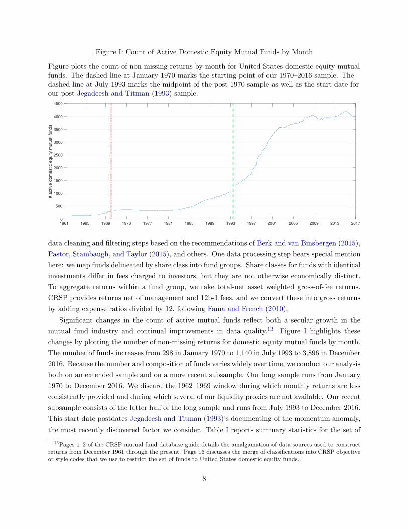
Figure I: Count of Active Domestic Equity Mutual Funds by Month
Figure plots the count of non-missing returns by month for United States domestic equity mutualfunds. The dashed line at January 1970 marks the starting point of our 1970–2016 sample. Thedashed line at July 1993 marks the midpoint of the post-1970 sample as well as the start date forour post-Jegadeesh and Titman (1993) sample.
1961 1965 1969 1973 1977 1981 1985 1989 1993 1997 2001 2005 2009 2013 20170
500
1000
1500
2000
2500
3000
3500
4000
4500
# a
ctiv
e d
om
est
ic e
qu
ity m
utu
al f
un
ds
data cleaning and filtering steps based on the recommendations of Berk and van Binsbergen (2015),Pastor, Stambaugh, and Taylor (2015), and others. One data processing step bears special mentionhere: we map funds delineated by share class into fund groups. Share classes for funds with identicalinvestments differ in fees charged to investors, but they are not otherwise economically distinct.To aggregate returns within a fund group, we take total-net asset weighted gross-of-fee returns.CRSP provides returns net of management and 12b-1 fees, and we convert these into gross returnsby adding expense ratios divided by 12, following Fama and French (2010).
Significant changes in the count of active mutual funds reflect both a secular growth in themutual fund industry and continual improvements in data quality.13 Figure I highlights thesechanges by plotting the number of non-missing returns for domestic equity mutual funds by month.The number of funds increases from 298 in January 1970 to 1,140 in July 1993 to 3,896 in December2016. Because the number and composition of funds varies widely over time, we conduct our analysisboth on an extended sample and on a more recent subsample. Our long sample runs from January1970 to December 2016. We discard the 1962–1969 window during which monthly returns are lessconsistently provided and during which several of our liquidity proxies are not available. Our recentsubsample consists of the latter half of the long sample and runs from July 1993 to December 2016.This start date postdates Jegadeesh and Titman (1993)’s documenting of the momentum anomaly,the most recently discovered factor we consider. Table I reports summary statistics for the set of
13Pages 1–2 of the CRSP mutual fund database guide details the amalgamation of data sources used to constructreturns from December 1961 through the present. Page 16 discusses the merge of classifications into CRSP objectiveor style codes that we use to restrict the set of funds to United States domestic equity funds.
8

Table I: Domestic Equity Mutual Fund Sample Summary Statistics
Table presents summary statistics for the 1970–2016 sample of 7,331 United States domestic equitymutual funds. The top subtable provides information on the time series of the number of activefunds for each date as well as cross-sectional information on fund lifetimes and total net assets(TNA) at sample start, middle, and end. The bottom subtable reports distributional informationon fund excess returns. ⇢̄ is the average pairwise correlation with other mutual funds’ returns, and⇢S&P500 is the correlation with the S&P 500.
Funds Lifetime TNA, Jan. 1970 TNA, July 1993 TNA, Dec. 2016Unit # Years Million USD Million USD Million USD
Mean 1901 146.2 129.79 436.02 1554.00Std. Dev. 1555 108.34 318.16 1337.10 6855.50
25% 357 64 3.81 30.47 49.8050% 1202 119 22.78 88.00 201.4075% 3724 200 89.60 290.26 861.70
Mean Return Return Vol. Sharpe Ratio ⇢̄MF ⇢S&P500
Unit % / Month % / Month Annualized % %
Mean 0.48 4.95 0.42 76.83 86.64Std. Dev. 0.62 1.86 0.43 16.28 18.09
25% 0.33 3.98 0.24 74.79 84.2850% 0.59 4.71 0.45 80.44 91.1375% 0.80 5.61 0.61 84.49 95.25
mutual funds used in our analysis. All told the 1970–2016 sample consists of 1,071,818 fund-monthobservations and the 1993–2016 sample consists of 929.446 fund-month observations.
Much of our analysis compares mutual funds with similar stocks as measured by loadings onequity risk factors. Our Fama-MacBeth tests of Section IV combine mutual fund data with commontest portfolios. Because our factor set includes value (HML), size (SMB), and momentum (UMD),our baseline analysis uses the Fama-French 25 size-value double-sorted portfolios plus 25 size-beta portfolios, 25 size-prior return portfolios, and 25 size-Amihud illiquidity portfolios to ensureadequate dispersion in loadings to identify risk premia in the cross section. We supplement thisset of test assets with an expanded cross section following the recommendation of Lewellen, Nagel,and Shanken (2010). In our larger portfolio set, we also include 49 industry portfolios, 25 size-operating profitability portfolios, 25 size-investment portfolios, 10 beta-sorted portfolios, 10 marketcapitalization-sorted portfolios, 10 book equity to market equity ratio sorted portfolios, 10 Amihudilliquidity-sorted portfolios, 10 operating profitability-sorted portfolios, and 10 investment-sortedportfolios for a total of 269 portfolios. With the exception of the illiquidity-sorted portfolios, all
9

portfolio data are downloaded from Ken French’s website. Decile illiquidity portfolios sort bymonthly averages of non-missing daily absolute returns over dollar volume, and stocks are assignedfor the following year using deciles the end of June, by parallel with the timing convention of theother portfolio data. The 25 size-illiquidity portfolios sort on both lagged market capitalizationand Amihud illiquidity quintile. Our analysis uses both equal- and value-weighted stock portfolios.
We include several market and funding liquidity variables to proxy for time-varying cost fac-tors that may affect the performance of mutual funds relative to stocks. Our market liquidityvariables are Amihud illiquidity (Amihud (2002)), Pastor-Stambaugh liquidity levels (Pastor andStambaugh (2003)), Corwin and Schultz (2012) NYSE-average bid-ask spreads, and the CBOE S&P500 Volatility Index (VIX), as motivated by Nagel (2012). We use Corwin and Schultz (2012)’smethodology to estimate bid-ask spreads because it enables measurement of market liquidity be-fore TAQ becomes available in 1993 and because it captures average effective spread levels andinnovations better than other pre-TAQ methodologies (see Corwin and Schultz (2012) Table IV).14
We use the CBOE S&P 100 Volatility Index (VXO) in place of the VIX in the pre-1990 period forwhich the VIX is not available. We compute Amihud illiquidity using CRSP daily data with valuesaveraged within a month as in Amihud (2002), and we obtain the Pastor-Stambaugh series andCBOE VXO/VIX series from Robert Stambaugh’s website and the Federal Reserve of St. Louis’sFRED database, respectively.
Our funding liquidity variables are Frazzini and Pedersen (2014)’s “betting against beta” (BAB)factor, He, Kelly, and Manela (2017)’s intermediary capital ratio, the 10-year BAA minus 10-yearTreasury spread, and the 3-month LIBOR minus 3-month Treasury yield or “TED” spread. Thefirst two series are expressly designed to capture institutions’ funding liquidity constraints, and thelatter two series are common proxies in the funding liquidity literature (e.g., Brunnermeier (2009)).We obtain BAB from AQR’s website, intermediary capital ratios from Asaf Manela’s website, andcredit and TED spreads from FRED.
IV. Fama-MacBeth Estimates of Implementation Costs
We measure the returns to factor investing using two approaches. In this section we considerthe compensation per unit of risk exposure and investigate whether mutual funds obtain the samerisk premium that academics achieve on paper. In the next section we evaluate the gross-of-feereturns to investing in factor portfolios of stocks and mutual funds with similar risk attributes.
14Corwin and Schultz make their code available at https://www3.nd.edu/⇠scorwin/HILOW_Estimator_Sample_002.sas.As in their paper, we compute cross-sectional averages using only NYSE-listed stocks, and we use their variant ofestimated spreads in which negative values are set to 0.
10
A. Baseline Estimates
In our baseline estimation, we assume that mutual funds have a constant per-unit cost for imple-menting academic anomalies. Investing in a market index with �MKT = 1 results in a performancegap of ⌘ relative to the on-paper performance of a market index, and investing in a levered versionof the market more generally results in a performance gap of ⌘�MKT . In this setting, we wouldexpect performance differences between stock and mutual fund portfolios to be linear in factorexposure.
We estimate the “implementation gap” using augmented Fama and MacBeth (1973) two-stageregressions for the Carhart four-factor model (Carhart (1997)). The time-series regression step isstandard except for the choice of test assets. As discussed in the preceding section, our sortingcharacteristics pertain to each factor in fkt, and we have NS = 100 and NS = 269 stock portfoliosdepending on regression specification. In addition to stock portfolios, we also include as testassets NMF = 7, 331 mutual funds, of which several thousand are active in the typical period. Asdiversified entities spanning a wide range of multifactor risk exposures, mutual funds unlike stocksneed not be grouped into portfolios via a characteristic-sorting procedure.
The NS +NMF time-series regressions are
rit = ↵i +X
k
fkt�ik + ✏it, i = 1, . . . , NS , NS+1, . . . , NS +NMF , (1)
where rit is the month t gross return on stock portfolio or mutual fund i net of the contemporaneousrisk-free rate and fkt (for k = 1, ...,K) is the return on factor k at date t. The usual second-stagecross-sectional regressions are extended to accommodate the possibility of differences in risk pricingfor stocks and mutual funds,
rit =X
k
�Skt�̂ik1i2S +
X
k
�MFkt �̂ik1i2MF + ✏it, t = 1, . . . , T. (2)
Regression (2) is equivalent to two separate cross-sectional regressions run on stocks and mutualfunds because the indicators partition the set of observations. �S
kt is the realized price of risk forfactor k and date t based on stock returns, and �MF
kt is the corresponding estimate based on mutualfund returns. The difference �̂�
kt ⌘ �̂Skt��̂MF
kt is our estimate of the implementation costs for strategyk: it is the difference between the on-paper profitability of a given strategy (“what you see”) andthe actual returns achieved by an asset manager facing real-world implementation costs (“what youget”).15 Conceptually this difference captures both direct costs such as spreads and price impactfrom factor trading as well as indirect costs such as investing in liquid versions of factors to robustifystrategies against outflows.16 Our point estimates are the average of the monthly differences in
15We account for potential cost asymmetries between funds with positive factor exposures and funds with negativefactor exposures in Section VII.A.
16Julian Robertson’s Tiger Management, one of the world’s largest hedge funds in the late 1990s, collapsed precisely
11

factor compensation �̄�k , and we construct standard errors for this difference using Newey and
West (1987) with three monthly lags to account for serial correlation and heteroskedasticity in the�-difference series.
Throughout our analysis, we estimate cross-sectional slopes of returns on risk exposures as-suming that risk exposures are constant. In making this assumption we prioritize minimizing theerrors-in-variables problem arising from using noisy betas as inputs in the second-stage Fama-MacBeth regression. This problem is vitally important because we do not want to find differencesin �s simply as a byproduct of higher measurement error in mutual fund betas. However, in usinglong estimation windows to estimate �s, we nonetheless take on potential measurement error arisingfrom time-variation in stock portfolio or mutual fund risk exposures.
Following Lettau, Maggiori, and Weber (2014) and others, we omit the constant term to forcecross-sectional average alphas to zero. Economically this omission forces the typical zero-risk se-curity or mutual fund to have zero excess (gross) return at each point in time. We impose thisrestriction because the slope on �MKT is not otherwise well identified in our stock portfolio sample,namely the time series of the intercept ↵t and the estimated market risk premium �MKT,t arestrongly negatively correlated and of similar magnitudes. By contrast in the mutual fund sample,�̂ik has a large and positive risk price regardless of whether a constant is included. None of theother factor risk premia are meaningfully affected.
Table II presents estimates of Equation (2). The �� value in the upper-left corner indicatesthat the difference in compensation per unit of market exposure is 0.26% per year greater forrisk exposures taken in practice via mutual funds than on paper in (100 equal-weighted) stockportfolios. This difference changes sign to favor on-paper portfolios by 0.34% per year when assessedagainst the full set of 269 portfolios because the average compensation for market beta is higherin the larger sample. Neither effect is statistically or economically significant, and the absence ofa performance gap is robust to using value-weighted portfolios (bottom panel) rather than equal-weighted portfolios. This result is unsurprising as mutual funds are expected to be relatively goodat implementing the market factor.
Broadening our focus to columns 1–4, we see that mutual funds underperform stocks in isolatingfactor exposures for two of the other Carhart factors. The average implementation gaps for value(HML) and momentum (UMD) range from of 50%–80% of the total on-paper return to eachfactor in stock portfolios. The remaining compensation to mutual funds for HML and UMD arepositive (�MF > 0), but they are only 1%–3% per year and not statistically distinguishable fromzero. Conversely, HML and UMD factors are both highly compensated and statistically robust inequal-weighted paper portfolios in this period. Compensation for size factor (SMB) exposure hasa small positive point estimate for mutual funds, but these values are not reliably different fromzero or from on-paper compensation for size.
because it could not continue to service outflows associated with its value investment strategy. Shleifer and Vishny(1997) formalize the role of agency frictions in perpetuating anomalies.
12
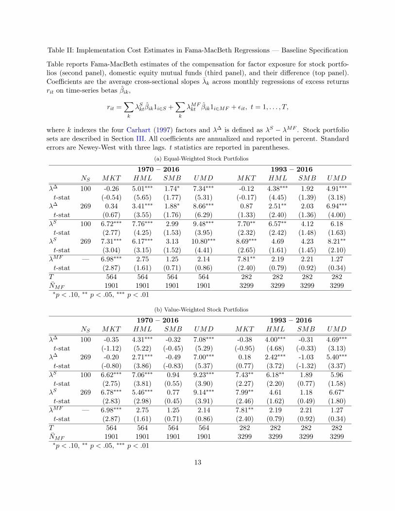
Table II: Implementation Cost Estimates in Fama-MacBeth Regressions — Baseline Specification
Table reports Fama-MacBeth estimates of the compensation for factor exposure for stock portfo-lios (second panel), domestic equity mutual funds (third panel), and their difference (top panel).Coefficients are the average cross-sectional slopes �̄k across monthly regressions of excess returnsrit on time-series betas �̂ik,
rit =X
k
�Skt�̂ik1i2S +
X
k
�MFkt �̂ik1i2MF + ✏it, t = 1, . . . , T,
where k indexes the four Carhart (1997) factors and �� is defined as �S � �MF . Stock portfoliosets are described in Section III. All coefficients are annualized and reported in percent. Standarderrors are Newey-West with three lags. t statistics are reported in parentheses.
(a) Equal-Weighted Stock Portfolios
1970 – 2016 1993 – 2016
NS MKT HML SMB UMD MKT HML SMB UMD
�� 100 -0.26 5.01⇤⇤⇤ 1.74⇤ 7.34⇤⇤⇤ -0.12 4.38⇤⇤⇤ 1.92 4.91⇤⇤⇤t-stat (-0.54) (5.65) (1.77) (5.31) (-0.17) (4.45) (1.39) (3.18)
�� 269 0.34 3.41⇤⇤⇤ 1.88⇤ 8.66⇤⇤⇤ 0.87 2.51⇤⇤ 2.03 6.94⇤⇤⇤t-stat (0.67) (3.55) (1.76) (6.29) (1.33) (2.40) (1.36) (4.00)
�S 100 6.72⇤⇤⇤ 7.76⇤⇤⇤ 2.99 9.48⇤⇤⇤ 7.70⇤⇤ 6.57⇤⇤ 4.12 6.18t-stat (2.77) (4.25) (1.53) (3.95) (2.32) (2.42) (1.48) (1.63)
�S 269 7.31⇤⇤⇤ 6.17⇤⇤⇤ 3.13 10.80⇤⇤⇤ 8.69⇤⇤⇤ 4.69 4.23 8.21⇤⇤t-stat (3.04) (3.15) (1.52) (4.41) (2.65) (1.61) (1.45) (2.10)
�MF — 6.98⇤⇤⇤ 2.75 1.25 2.14 7.81⇤⇤ 2.19 2.21 1.27t-stat (2.87) (1.61) (0.71) (0.86) (2.40) (0.79) (0.92) (0.34)
T 564 564 564 564 282 282 282 282N̄MF 1901 1901 1901 1901 3299 3299 3299 3299⇤p < .10, ⇤⇤ p < .05, ⇤⇤⇤ p < .01
(b) Value-Weighted Stock Portfolios
1970 – 2016 1993 – 2016
NS MKT HML SMB UMD MKT HML SMB UMD
�� 100 -0.35 4.31⇤⇤⇤ -0.32 7.08⇤⇤⇤ -0.38 4.00⇤⇤⇤ -0.31 4.69⇤⇤⇤t-stat (-1.12) (5.22) (-0.45) (5.29) (-0.95) (4.68) (-0.33) (3.13)
�� 269 -0.20 2.71⇤⇤⇤ -0.49 7.00⇤⇤⇤ 0.18 2.42⇤⇤⇤ -1.03 5.40⇤⇤⇤t-stat (-0.80) (3.86) (-0.83) (5.37) (0.77) (3.72) (-1.32) (3.37)
�S 100 6.62⇤⇤⇤ 7.06⇤⇤⇤ 0.94 9.23⇤⇤⇤ 7.43⇤⇤ 6.18⇤⇤ 1.89 5.96t-stat (2.75) (3.81) (0.55) (3.90) (2.27) (2.20) (0.77) (1.58)
�S 269 6.78⇤⇤⇤ 5.46⇤⇤⇤ 0.77 9.14⇤⇤⇤ 7.99⇤⇤ 4.61 1.18 6.67⇤t-stat (2.83) (2.98) (0.45) (3.91) (2.46) (1.62) (0.49) (1.80)
�MF — 6.98⇤⇤⇤ 2.75 1.25 2.14 7.81⇤⇤ 2.19 2.21 1.27t-stat (2.87) (1.61) (0.71) (0.86) (2.40) (0.79) (0.92) (0.34)
T 564 564 564 564 282 282 282 282N̄MF 1901 1901 1901 1901 3299 3299 3299 3299⇤p < .10, ⇤⇤ p < .05, ⇤⇤⇤ p < .01
13

Notably the point estimates for the differences �� for HML and UMD are typically morestatistically significant than either of the components of the difference �S or �MF . This featurereflects the netting out of common variation in factor realizations within each cross section. Ideallythe residual variation in �� captures only random variation in trading costs. In practice thisresidual variation also captures idiosyncratic differences in estimated risk prices associated withusing different sets of test assets; the difference between �� estimated from the set of 100 stockportfolios and the set of 269 stock portfolios suggests that the implementation gap depends in parton the stock benchmarks employed.
Columns 5–8 reproduce these tests for the July 1993 to December 2016 sample. Mutual fundsachieve lower returns to HML and UMD and higher returns to SMB than in the full sample,but these returns are now universally statistically indistinguishable from zero (in part because thesample length is cut in half). For stock portfolios, the compensation for HML and UMD (SMB)exposures also decrease (increase) relative to the full sample. The net effect of these changes isa small decrease in the typical implementation gap for HML and a moderate decrease in theimplementation gap for UMD. The implementation gap is roughly unchanged for market exposure(effectively zero) and SMB exposure (positive but insignificant). In sum, focusing on the lattersample with a more broadly representative set of mutual funds does not change our conclusionson the high real-world efficacy of implementing market exposure and size and the low real-worldefficacy of implementing value and momentum.
B. Time- and Mutual-Fund Varying Per-Unit Cost Estimates
Time-varying implementation costs complicate the comparison of compensation per unit offactor risk. To see why, consider the following augmented model of mutual fund costs. As before,let there be a set of academic factors f , where ft is a 1⇥K vector. Each mutual fund i implementsits favored version of academic factors and earns a return of
hit = ft � ⌘it, (3)
where ⌘it reflects tilts away from the academic factor on account of trading costs or factor opti-mization. This section differs from the previous one in that we no longer assume that ⌘ is constantacross funds and time. The ⌘it term in turn has components
⌘it = ⌘i + ⌘t�i + ⌘̃it. (4)
The first component is the fixed, firm-specific cost of trading a factor. The second component isthe set of L time-varying liquidity costs ⌘t multiplied by the L⇥K loadings of all factors on theseliquidity costs �i. Finally, ⌘̃it is a 1⇥K set of idiosyncratic costs, e.g., a surprise liquidity demandshock that thwarts or facilitates firm i’s trading strategy for factor k.
14

Funds trade and earn returns
rit = ↵i + hit�i + ✏it = (↵i � ⌘i�i) + (ft � ⌘t�i)�i + (✏it � ⌘̃it�i) . (5)
An ideal test compares the average compensation ft for factor exposure for on-paper investment instocks against the compensation hit for factor exposure for real-world investment through invest-ment managers. In the constant-cost setting of Section IV.A, we achieve this ideal: ⌘it simplifiesto ⌘, and Fama-MacBeth regressions with a K-factor model recovers consistent estimates of f � h
as in Equation (2).By contrast, in this general setting we face two key challenges that complicate the straightfor-
ward comparison of ft and hit. First, trading costs vary over time, and these costs may covarywith factor realizations. For example, several measures of funding and market liquidity deterioratesignificantly during the 2007–2008 Financial Crisis, and the aggregate market return likewise isconsistently negative at that time. Omitting relevant liquidity factors thus contributes to an omit-ted variable bias in time-series estimates of �i for investment managers, which in turn potentiallyinvalidates simple comparisons of second-stage slope estimates. Second, investment managers selecttheir risk exposures endogenously. An investor who has discovered improvements upon academicfactors or is particularly skilled at trading a given factor cost-effectively is more likely to select alarger factor exposure, all else equal. For this reason we would expect mutual fund-specific tradinggains ⌘i to be increasing in �i, and the cross-sectional slopes of returns with respect to �i are biasedupward (�̂MF
t > �MFt ).
We now address these two sources of bias. To address the omission of trading cost factors, weassume that trading costs or optimization gains for mutual funds are spanned by liquidity proxiesconsidered in the literature and discussed in Section III. Throughout we use liquidity levels ratherthan innovations because high illiquidity rather than increases in illiquidity relative to the previ-ous month likely contribute to high factor implementation costs.17 We then run Fama-MacBethregressions as before, but we extend the factor model to include liquidity proxies in the time-seriesregressions,
rit = ↵i +X
k
fkt�ik +X
l
⌘̃lt�̃il + ✏it, i = 1, . . . , NS , NS+1, . . . , NS +NMF , (6)
where ⌘̃lt are the liquidity factor proxies at time t. To avoid overfitting in the first stage byincluding too many correlated liquidity proxies, we start with two:18 the first principal componentof four market liquidity variables (Amihud illiquidity, Pastor-Stambaugh liquidity, Corwin-Schultz
17By contrast, if we sought to explain returns, innovations to liquidity expectations would be the correct variableto use (as emphasized by Pastor and Stambaugh (2003) and He, Kelly, and Manela (2017), among others).
18Ideally we would use all liquidity variables rather than their principal components because we want time-varyingdeterminants of ⌘it to lie in the span of the liquidity-augmented factor model. To this end we include all proxies ina sparse regression approach in Appendix C.
15

bid-ask spreads and the CBOE VIX/VXO) and the first principal component of four fundingliquidity variables (Frazzini and Pedersen (2014)’s “betting against beta” factor, He, Kelly, andManela (2017)’s intermediary capital risk factor, 10-year BAA minus 10-year Treasury spreads,and 3-month LIBOR minus 3-month Treasury yield or “TED” spreads). We normalize all liquidityvariables to have unit standard deviation before taking principal components because liquidityproxies vary widely in their scales.19
The second-stage cross-sectional regressions are exactly as in Equation (2). The mismatch inmodel specification for the time-series and cross-sectional regressions is intentional. In the time-series regressions, we recover fund exposures to the academic factors, and we need the additionalliquidity proxy variables to cleanse the estimated mutual fund factor loadings of omitted illiquiditycomponents. By contrast, in the second stage, we recover the cost per unit exposure to the academicfactors and do not want to include the liquidity proxy exposures. Excluding the liquidity factorsonly in the second stage delivers �̂S
t = �St and
�̂�t = �S
t �cov
�rMFit ,�i
�
var (�i)= �cov (↵i � ⌘it�i,�i)
var (�i)= ⌘̄t �
cov ((⌘̄t � ⌘it)�i,�i)
var (�i). (7)
The final equality makes the standard assumption that alphas and betas are cross-sectionally un-correlated. ⌘̄t represents the cross-sectional average per-unit liquidity costs to implementing thefactor. The second term is the covariance between deviations from the average costs and �s. Fundswith a particular skill in investing in a factor likely have higher exposures to it—�i are endoge-nous—so �i is high when ⌘̄t � ⌘it is high, and �i is close to zero when ⌘̄t � ⌘it is negative (negativebetas do not reverse the sign on costs). Combining these features, the overall covariance is posi-tive.20 Consequently �MF
kt is an upper bound on the realizable gains to factor investing per unitrisk exposure, and ��
kt is a lower bound on the costs of implementing a factor strategy.Table III reports results using the liquidity-extended first-stage regression. Results are virtually
the same as those of the baseline specification in Table II with one exception. Mutual funds’ (alreadylow) annual compensation for UMD exposure decreases from 2.14% to 1.98% in the long sampleand from 1.27% to 0.27% in the recent sample, suggesting that liquidity factor exposure at leastpartly explains mutual funds’ compensation for momentum. This finding extends one result ofAsness, Moskowitz, and Pedersen (2013) to the universe of mutual funds. Asness, Moskowitz, andPedersen (2013) find that momentum loads positively on liquidity risk, and we find that the same
19The CBOE VXO and the TED spread series start in January 1986. Our principal components procedure accom-modates the missing liquidity proxy data using MATLAB’s alternating least squares (ALS) algorithm. ALS extractsfactors and completes missing data by conjecturing principal components and iteratively estimating principal com-ponent loadings � and factor values g until the distance between known and fitted values achieves a local minimum.We run PCA-ALS from 1,000 starting points and select the global distance-minimizing factors and loadings. By con-struction illiquidity principal components have unit standard deviation, and we assign these components an illiquidityinterpretation by normalizing them to be positively correlated with the VIX/VXO.
20Including liquidity proxies in the second-stage introduces a more opaque omitted variable bias, as we discuss inAppendix B.
16

Table III: Implementation Cost Estimates in Fama-MacBeth Regressions — Liquidity PCs
Table reports Fama-MacBeth estimates of the compensation for factor exposure for stock portfo-lios (second panel), domestic equity mutual funds (third panel), and their difference (top panel).Coefficients are the average cross-sectional slopes �̄k across monthly regressions of excess returnsrit on time-series betas �̂ik,
rit =X
k
�Skt�̂ik1i2S +
X
k
�MFkt �̂ik1i2MF + ✏it, t = 1, . . . , T,
where k indexes the four Carhart (1997) factors and �� is defined as �S � �MF . First-stageregression estimates include these factors, the first principal component of market liquidity proxies,and the first principal component of funding liquidity proxies. Liquidity proxies and stock portfoliosets are described in Section III. All coefficients are annualized and reported in percent. Standarderrors are Newey-West with three lags. t statistics are reported in parentheses.
(a) Equal-Weighted Stock Portfolios
1970 – 2016 1993 – 2016
NS MKT HML SMB UMD MKT HML SMB UMD
�� 100 -0.43 5.27⇤⇤⇤ 2.06⇤⇤ 7.51⇤⇤⇤ -0.06 4.11⇤⇤⇤ 1.97 5.57⇤⇤⇤t-stat (-0.90) (5.81) (2.10) (5.34) (-0.08) (3.97) (1.46) (3.27)
�� 269 0.15 3.85⇤⇤⇤ 2.29⇤⇤ 8.73⇤⇤⇤ 0.78 2.56⇤⇤ 2.20 6.99⇤⇤⇤t-stat (0.30) (3.86) (2.14) (6.13) (1.17) (2.37) (1.54) (3.72)
�S 100 6.55⇤⇤⇤ 8.06⇤⇤⇤ 3.22⇤ 9.49⇤⇤⇤ 7.77⇤⇤ 5.97⇤⇤ 4.22 5.84t-stat (2.71) (4.34) (1.67) (3.97) (2.35) (2.20) (1.54) (1.54)
�S 269 7.13⇤⇤⇤ 6.64⇤⇤⇤ 3.45⇤ 10.71⇤⇤⇤ 8.61⇤⇤⇤ 4.42 4.46 7.26⇤t-stat (2.99) (3.31) (1.69) (4.38) (2.65) (1.50) (1.57) (1.85)
�MF — 6.98⇤⇤⇤ 2.79 1.16 1.98 7.83⇤⇤ 1.86 2.26 0.27t-stat (2.88) (1.62) (0.66) (0.80) (2.41) (0.67) (0.93) (0.07)
T 564 564 564 564 282 282 282 282N̄MF 1901 1901 1901 1901 3299 3299 3299 3299⇤p < .10, ⇤⇤ p < .05, ⇤⇤⇤ p < .01
(b) Value-Weighted Stock Portfolios
1970 – 2016 1993 – 2016
NS MKT HML SMB UMD MKT HML SMB UMD
�� 100 -0.43 4.70⇤⇤⇤ -0.24 7.30⇤⇤⇤ -0.38 4.35⇤⇤⇤ -0.34 5.69⇤⇤⇤t-stat (-1.36) (5.55) (-0.33) (5.40) (-0.94) (5.00) (-0.36) (3.48)
�� 269 -0.21 2.99⇤⇤⇤ -0.45 7.15⇤⇤⇤ 0.18 2.77⇤⇤⇤ -1.01 6.24⇤⇤⇤t-stat (-0.83) (4.03) (-0.76) (5.46) (0.78) (4.09) (-1.30) (3.73)
�S 100 6.56⇤⇤⇤ 7.49⇤⇤⇤ 0.92 9.28⇤⇤⇤ 7.45⇤⇤ 6.21⇤⇤ 1.91 5.96t-stat (2.73) (3.99) (0.54) (3.93) (2.29) (2.19) (0.78) (1.58)
�S 269 6.78⇤⇤⇤ 5.78⇤⇤⇤ 0.71 9.13⇤⇤⇤ 8.01⇤⇤ 4.63 1.24 6.52⇤t-stat (2.83) (3.11) (0.42) (3.90) (2.48) (1.60) (0.51) (1.76)
�MF — 6.98⇤⇤⇤ 2.79 1.16 1.98 7.83⇤⇤ 1.86 2.26 0.27t-stat (2.88) (1.62) (0.66) (0.80) (2.41) (0.67) (0.93) (0.07)
T 564 564 564 564 282 282 282 282N̄MF 1901 1901 1901 1901 3299 3299 3299 3299⇤p < .10, ⇤⇤ p < .05, ⇤⇤⇤ p < .01 17
holds for mutual funds’ implementation of momentum. We examine this feature in detail in SectionVI.B.
V. Matched Pairs Estimates of Implementation Costs
The cross-sectional approach of the previous section compares the return compensation for anincremental unit of risk exposure taken in on-paper portfolios versus in mutual funds. Such anapproach does not address the question of whether large investments by mutual funds achieve morefavorable risk-reward trade-offs than marginal factor investments. For example, mutual funds mayexcel at taking on moderate risk exposures to a factor, but their performance may deterioratefor extreme exposures for which taking on additional leverage is needed (Frazzini and Pedersen(2014)). To answer this question, we consider the building blocks for many tradeable return factorsin academia—long-short portfolios implied by characteristic sorts—and conduct a matched pairsanalysis of characteristic-sorted stocks and matched mutual funds.21
A. Matched Pairs Methodology
We begin by constructing characteristics for each stock and sorting stocks into quintile portfolios.Our characteristics are 60-month rolling market beta (requiring at least 24 observations), book-to-market ratio,22 market capitalization (with scale reversed to place small stocks in the top quintile),and prior return over the previous year, skipping the latest month (the “2-12” return). We followthe methodology of Ken French’s website in constructing these characteristics, and we use theprovided breakpoints based on NYSE quintiles where available. In the case of rolling market betaswe construct our own quintile breakpoints. For the first three characteristics, we assign portfolios atthe end of June and retain assignments for July through the end of the following June. Momentumis a higher-frequency anomaly, and we sort on prior returns and retain assignments for the nextmonth only. We then estimate two sets of betas on monthly return data for all common stocks inthe CRSP universe and all U.S. domestic equity mutual funds: univariate betas with respect to asingle factor fk and multivariate betas with respect to all four Carhart factors.
For each stock in quintile q for factor k in month t, we find the three closest mutual funds activein that month. We assess proximity using the Mahalanobis distance on betas with covariancesestimated using the full sample,23 where �k determines distance in our univariate analysis, all four
21Our analysis is similar in spirit to Daniel, Grinblatt, Titman, and Wermers (1997), who examine the origins ofmutual fund performance by comparing mutual fund returns against those of characteristic-matched portfolios ofstocks. Rather than using holdings data to build and match with benchmark portfolios, we use a formal matchedpairs approach to directly compare mutual funds and stocks with similar multifactor betas.
22We source our book-to-market ratios from the WRDS Financial Ratios Suite. We make small modifications tothe provided code to extend the ratios to all stocks through the end of 2016.
23The Mahalanobis distance isp
(x� y)0 ⌃�1 (x� y) for two vectors x and y and covariance matrix ⌃. When ⌃ isdiagonal, it normalizes each dimension to have a unit standard deviation, and we adopt this terminology in the maintext. It reduces to the Euclidean distance when ⌃ = I.
18

�s determine distance in our multivariate analysis. Implicitly we select stocks as our matchedpairs “treatment group” because we want to mimic on-paper factor portfolios as best as possibleusing mutual funds. Each stock is matched to three mutual funds rather than one to improveprecision of the average return for mutual funds with the same risk characteristics. To ensure highmatch quality, we impose a maximum distance or caliper of 0.25 standard deviations for univariatematches (following Rosenbaum and Rubin (1984)’s rule-of-thumb in the context of propensity scorematching) and 0.25 ⇥ 4 = 1 standard deviation for four-factor matching. Stocks with fewer thanthree matched mutual funds within these radii are dropped.
We follow Abadie and Imbens (2006, 2011) to establish a bias-adjusted matched pairs estimatorfor each month’s implementation gap by calculating the average difference between next-monthreturns for stocks and mutual funds. Armed with monthly implementation gap estimates, wetake the average value as our full-sample estimate. We also consider differences in value-weightedreturns within each month using the lagged market capitalization of the matched stocks. AppendixD provides a detailed description of the matched pairs methodology and evaluation of match quality.
Our analysis includes univariate and multivariate matches because each mimics a differentstandard asset pricing approach and because each method entails making a particular set of trade-offs. Intuitively, matching on univariate betas answers the question of whether mutual funds arecomparably good as stocks at isolating a particular characteristic; for example, do mutual fundswith high (low) “value” betas achieve the same excess returns as high (low) value beta stocks? Thisanalysis parallels a comparison between Q5–Q1 returns from two standard portfolio sorts, where oneset of test assets (mutual funds) is transformed to have as similar risk attributes as possible to theother set of test assets (stocks). In favor of univariate matching is its high match rate and accuratematches along the dimension of interest, and this approach dominates when one matching feature ismore important than others in determining stock and mutual fund returns. Matching on all betasanswers the same question when excess returns are assessed with respect to a richer, nonparametricmodel that controls for possible variation in other risk factors. This multivariate-beta matchingapproach parallels multifactor tests such as Fama-MacBeth cross-sectional regressions in whichwe assess the returns to a single factor holding all other factors fixed. In favor of multivariatematching is its ability to simultaneously control for several determinants of returns to conduct atrue “all else equal” analysis for stocks and mutual funds. This approach—which we favor in ourapplication—trades off match quality in the dimension of interest with an elimination of systematicbiases in the other dimensions. We discuss trade-offs of each approach in more detail in AppendixD.B.
For each matched pairs analysis, we compare the performance of stocks in high-characteristicportfolios and matched mutual funds. These differences in high-characteristic quintile returns rep-resent a lower bound on the underperformance of mutual fund implementations of factor investing.
19

To see why, consider the difference in factor returns for stocks and mutual funds,
rS � rMF =⇣rlongS � rshortS
⌘�⇣rlongMF � rshortMF
⌘�⇣rlongS � rshortS
⌘�⇣rlongMF � rshortS
⌘= rlongS � rlongMF .
(8)The inequality in Equation (8) holds if mutual funds are weakly less able to implement the shortside of strategies than paper shorting returns would indicate. We expect underperformance onselling the low-beta quintiles because shorting entails relatively high transaction costs. Short-sideunderperformance is especially plausible if we find that mutual funds also underperform on thelong side. In addition, some firms implement positive-cost versions of anomalies such as long-onlymomentum, in which only the extreme “buy” portfolio is traded.
Note that we do not directly compare the performance of long-short strategies for stocks andmutual funds. We cannot short mutual funds, and underperformance on both ends of a long-shortstrategy, for example, because of transactions costs, would be incorrectly obscured by differencing,as such costs are additive. Instead, we settle for comparing performance on the long portfolios toestablish a lower bound on the implementation costs of asset pricing factors.
B. Results
Table IV reports the results of our matched pairs analysis. The �LMS value in the upper-leftcorner indicates that mutual funds underperform stocks with the same market beta exposure by2.5% per year when stocks are in the 60–80th percentile of the distribution of rolling market betas.We designate “LMS” as long high-market beta stocks and short low-market beta stocks to distinguishlong-short market beta portfolios from the equity premium Rm � Rf . This implementation gapis larger than the on-paper return to an equal-weighted long-short strategy based on market betaquintiles, and roughly 40% of the annual equity premium over this period (6.35% per year, nottabulated). Moving to the next column on the right, mutual funds continue to underperform stocksby a much-smaller 1.0% per year, and this value is no longer statistically significant. Moving downthe upper-left panel we see that the implementation gap is positive and statistically significant forall non-market factors considered. Costs are particularly high for momentum strategies, as priorliterature suggests, and they are similarly high for value strategies.
The smaller point estimates in quintile four relative to quintile five is a common feature through-out the panels, and it reflects the balance of two competing forces. On one side, if per-unit costsare fixed across firms (as in Section IV.A), higher betas translate into higher total implementationgaps � (h� f). On the other side, mutual funds select into the highest � group, so high-� groupmembership likely reflects lower per-unit underperformance h � f . For these reasons the productof � (h� f) could increase or decrease as we move to more extreme � quintiles, and empirically,the scale effect tends to dominate the selection effect.
The upper-left panel reflects performance differences between stocks and mutual funds matched
20

Tabl
eIV
:Ret
urns
ofM
atch
edSt
ocks
and
Mat
ched
Mut
ualF
unds
Tabl
esre
port
diffe
renc
esin
perf
orm
ance
betw
een
stoc
ksan
dm
atch
edm
utua
lfun
ds.
The
first
two
colu
mns
ofea
chpa
neld
enot
eth
edi
ffere
nce
inre
turn
sbe
twee
nst
ocks
and
mut
ual
fund
sin
quin
tile
sfo
ur(�
(4))
and
five
(�(5))
ofth
edi
stri
buti
onof
stoc
kch
arac
teri
stic
s.D
iffer
ence
sar
ees
tim
ated
usin
gm
atch
edpa
irs
onth
efo
urC
arha
rt(1
997)
fact
ors
wit
hbi
asad
just
men
tby
linea
rre
gres
sion
inth
em
atch
ing
vari
able
(s),
whe
rew
ede
sign
ate
“LM
S”as
long
high
-mar
ket
beta
stoc
ksan
dsh
ort
low
-mar
ket
beta
stoc
ksto
dist
ingu
ish
long
-sho
rtm
arke
tbe
tapo
rtfo
lios
from
the
equi
typr
emiu
mR
m�R
f.
Diff
eren
ces
are
equa
l-or
valu
e-w
eigh
ted
wit
hin
each
mon
than
dav
erag
edac
ross
mon
ths.
S(5
�1)
colu
mns
deno
teth
edi
ffere
nce
ineq
ual-
orva
lue-
wei
ghte
dpe
rfor
man
cebe
twee
nst
ocks
inqu
intile
s5
and
1of
the
dist
ribu
tion
ofch
arac
teri
stic
s.A
llco
effici
ents
are
annu
aliz
edan
dre
port
edin
perc
ent,
and
stan
dard
erro
rsar
eN
ewey
-Wes
tw
ith
thre
ela
gs.
The
first
pane
lmat
ches
only
on�k,w
here
asth
ese
cond
pane
lmat
ches
onal
lfo
urfa
ctor
s.C
olum
ns1–
6eq
ual
wei
ght
retu
rns,
and
colu
mns
7–12
valu
ew
eigh
tre
turn
sby
lagg
edm
arke
tca
pita
lizat
ion.
tst
atis
tics
are
repo
rted
inpa
rent
hese
s.(a
)So
rtin
gan
dM
atch
ing
onU
niva
riat
eB
eta
Equ
alW
eigh
ted
Val
ueW
eigh
ted
1970
–2016
1993
–2016
1970
–2016
1993
–2016
�(4)
�(5)
S(5
�1)
�(4)
�(5)
S(5
�1)
�(4)
�(5)
S(5
�1)
�(4)
�(5)
S(5
�1)
�LM
S2.
50⇤
1.01
-0.7
04.
41⇤⇤
2.84
2.26
-1.0
1-2
.53⇤
⇤-0
.63
0.24
-0.6
12.
32t-
stat
(1.6
5)(0
.49)
(-0.
23)
(2.0
1)(0
.92)
(0.4
7)(-
1.00
)(-
2.00
)(-
0.18
)(0
.16)
(-0.
33)
(0.4
4)�
HM
L5.
10⇤⇤
⇤9.
14⇤⇤
⇤11
.32⇤
⇤⇤4.
54⇤⇤
8.57
⇤⇤⇤
10.2
9⇤⇤⇤
1.39
3.74
⇤⇤⇤
4.77
⇤⇤-0
.71
0.55
1.51
t-st
at(3
.69)
(4.6
9)(5
.82)
(2.5
7)(3
.43)
(3.6
7)(1
.60)
(2.8
9)(2
.32)
(-0.
73)
(0.3
3)(0
.52)
�SM
B3.
07⇤⇤
⇤3.
63⇤⇤
3.82
2.88
3.61
4.00
3.06
⇤⇤⇤
1.62
1.61
2.78
1.52
2.34
t-st
at(2
.76)
(2.3
5)(1
.55)
(1.6
2)(1
.49)
(1.2
5)(2
.79)
(1.2
2)(0
.69)
(1.5
8)(0
.71)
(0.7
4)�
UM
D5.
96⇤⇤
⇤8.
12⇤⇤
⇤6.
17⇤⇤
6.40
⇤⇤⇤
7.06
⇤⇤⇤
1.91
2.24
⇤⇤3.
88⇤⇤
⇤8.
75⇤⇤
⇤2.
183.
43⇤
4.47
t-st
at(5
.74)
(5.6
1)(2
.32)
(4.2
7)(3
.44)
(0.4
3)(2
.16)
(3.2
3)(3
.00)
(1.4
4)(1
.91)
(1.0
0)⇤ p
<.10,
⇤⇤p<
.05,
⇤⇤⇤p<
.01
(b)
Sort
ing
and
Mat
chin
gon
Mul
tiva
riat
eB
etas
Equ
alW
eigh
ted
Val
ueW
eigh
ted
1970
–2016
1993
–2016
1970
–2016
1993
–2016
�(4)
�(5)
S(5
�1)
�(4)
�(5)
S(5
�1)
�(4)
�(5)
S(5
�1)
�(4)
�(5)
S(5
�1)
�LM
S2.
86⇤⇤
⇤3.
55⇤⇤
⇤-0
.70
4.44
⇤⇤⇤
5.69
⇤⇤⇤
2.26
-0.7
2-0
.40
-0.6
31.
293.
03⇤
2.32
t-st
at(4
.57)
(3.5
1)(-
0.23
)(5
.21)
(3.6
2)(0
.47)
(-1.
04)
(-0.
37)
(-0.
18)
(1.5
5)(1
.92)
(0.4
4)�
HM
L3.
99⇤⇤
⇤7.
58⇤⇤
⇤11
.32⇤
⇤⇤4.
18⇤⇤
⇤7.
69⇤⇤
⇤10
.29⇤
⇤⇤0.
073.
30⇤⇤
⇤4.
77-0
.05
3.19
⇤⇤⇤
1.51
t-st
at(6
.36)
(8.3
8)(5
.82)
(5.2
3)(6
.56)
(3.6
7)(0
.11)
(3.9
3)(2
.32)
(-0.
06)
(2.9
0)(0
.52)
�SM
B3.
54⇤⇤
⇤5.
86⇤⇤
⇤3.
824.
07⇤⇤
⇤5.
88⇤⇤
⇤4.
003.
39⇤⇤
⇤4.
03⇤⇤
⇤1.
613.
92⇤⇤
⇤4.
28⇤⇤
⇤2.
34t-
stat
(5.2
2)(6
.83)
(1.5
5)(4
.60)
(4.9
5)(1
.25)
(5.0
4)(5
.49)
(0.6
9)(4
.50)
(4.0
8)(0
.74)
�UM
D5.
05⇤⇤
⇤6.
68⇤⇤
⇤6.
17⇤⇤
5.51
⇤⇤⇤
6.21
⇤⇤⇤
1.91
1.84
⇤⇤⇤
2.19
⇤⇤8.
75⇤⇤
⇤1.
89⇤⇤
2.89
⇤⇤4.
47t-
stat
(9.3
0)(8
.76)
(2.3
2)(7
.60)
(5.9
8)(0
.43)
(2.6
0)(2
.22)
(3.0
0)(2
.23)
(2.2
5)(1
.00)
⇤ p<
.10,
⇤⇤p<
.05,
⇤⇤⇤p<
.01
21
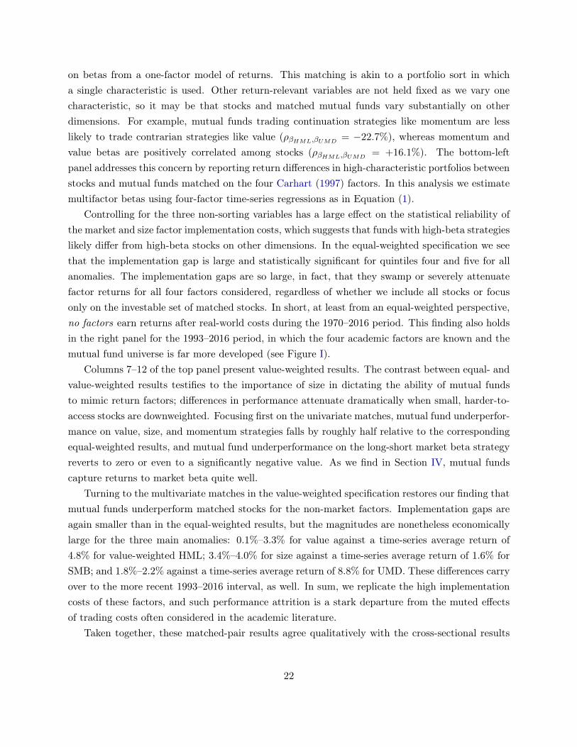
on betas from a one-factor model of returns. This matching is akin to a portfolio sort in whicha single characteristic is used. Other return-relevant variables are not held fixed as we vary onecharacteristic, so it may be that stocks and matched mutual funds vary substantially on otherdimensions. For example, mutual funds trading continuation strategies like momentum are lesslikely to trade contrarian strategies like value (⇢�HML,�UMD
= �22.7%), whereas momentum andvalue betas are positively correlated among stocks (⇢�HML,�UMD
= +16.1%). The bottom-leftpanel addresses this concern by reporting return differences in high-characteristic portfolios betweenstocks and mutual funds matched on the four Carhart (1997) factors. In this analysis we estimatemultifactor betas using four-factor time-series regressions as in Equation (1).
Controlling for the three non-sorting variables has a large effect on the statistical reliability ofthe market and size factor implementation costs, which suggests that funds with high-beta strategieslikely differ from high-beta stocks on other dimensions. In the equal-weighted specification we seethat the implementation gap is large and statistically significant for quintiles four and five for allanomalies. The implementation gaps are so large, in fact, that they swamp or severely attenuatefactor returns for all four factors considered, regardless of whether we include all stocks or focusonly on the investable set of matched stocks. In short, at least from an equal-weighted perspective,no factors earn returns after real-world costs during the 1970–2016 period. This finding also holdsin the right panel for the 1993–2016 period, in which the four academic factors are known and themutual fund universe is far more developed (see Figure I).
Columns 7–12 of the top panel present value-weighted results. The contrast between equal- andvalue-weighted results testifies to the importance of size in dictating the ability of mutual fundsto mimic return factors; differences in performance attenuate dramatically when small, harder-to-access stocks are downweighted. Focusing first on the univariate matches, mutual fund underperfor-mance on value, size, and momentum strategies falls by roughly half relative to the correspondingequal-weighted results, and mutual fund underperformance on the long-short market beta strategyreverts to zero or even to a significantly negative value. As we find in Section IV, mutual fundscapture returns to market beta quite well.
Turning to the multivariate matches in the value-weighted specification restores our finding thatmutual funds underperform matched stocks for the non-market factors. Implementation gaps areagain smaller than in the equal-weighted results, but the magnitudes are nonetheless economicallylarge for the three main anomalies: 0.1%–3.3% for value against a time-series average return of4.8% for value-weighted HML; 3.4%–4.0% for size against a time-series average return of 1.6% forSMB; and 1.8%–2.2% against a time-series average return of 8.8% for UMD. These differences carryover to the more recent 1993–2016 interval, as well. In sum, we replicate the high implementationcosts of these factors, and such performance attrition is a stark departure from the muted effectsof trading costs often considered in the academic literature.
Taken together, these matched-pair results agree qualitatively with the cross-sectional results
22
for three of the four factors (MKT/LMS, HML, and UMD), but they disagree for size. Thisdisagreement is likely attributable to the fact that SMB beta is not associated with cross-sectionaldifferences in average returns—and the cross-sectional approach thus reveals no difference in com-pensation to SMB exposure—whereas the small-size characteristic is associated with higher aver-age returns. Consequently we observe high returns on small-stock portfolios in the matched pairsapproach, and mutual funds clearly cannot capture these returns well in practice.
VI. Cost Estimates Over Time and Across Funds
A. Comparison with Previous Implementation Cost Estimates
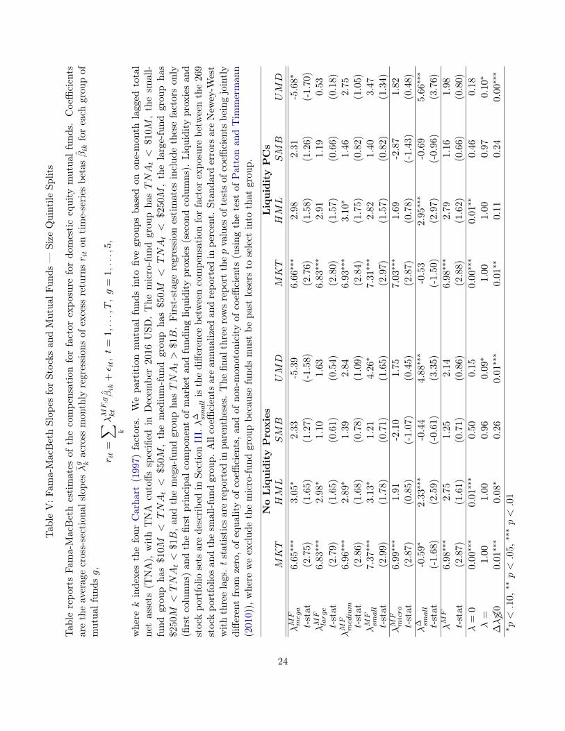
Our analysis thus far considers the implementation costs of factor strategies for representativemutual funds, with no attention paid to heterogeneous characteristics and costs. Variation ininvestors’ trading technologies may drive a wedge between a typical asset manager and the marginalinvestor in an anomaly, and by dividing asset managers into groups we can learn whether factorsare broadly (in)accessible or whether they generate positive net-of-costs returns for a subset ofmanagers. In this section, we briefly demonstrate the utility of our cross-sectional approach forexamining segments of asset managers.
Motivated by extensive work relating fund size to gross-of-fees performance (e.g., Berk andGreen (2004), Pastor, Stambaugh, and Taylor (2015), and Berk and van Binsbergen (2015)), wesplit fund groups into groups based on lagged total net assets (TNA), analogous to the R2 splitsin the previous section. We then run our second-stage cross-sectional regressions (2) separately foreach asset manager TNA group.24 We set aside funds with less than $10 million in assets becauseselection into this group implies that the fund has lost money (recall that we retain observationsonly after funds reach $10 million in assets to avoid incubation bias).25
Table V presents results from these segmented regressions on the full 1970–2016 sample. Asin Tables II–A.I, mutual funds generally achieve returns to market factor exposure comparable tothose of on-paper stock portfolios. HML also earns positive compensation for most TNA groups,and returns to HML are collectively different from zero in all specifications. Micro funds driveour finding of low overall mutual fund compensation for value. Point estimates for returns toSMB are positive for all fund size groups, but SMB compensation estimates are not statisticallydistinguishable from zero or from each other.
24Groups are assigned separately for each date with cutoffs based on December 2016 USD. The micro-fund grouphas TNAt < $10M and comprises 5.2% of the data. This group is selected in that it consists of past losers whoseassets had at one time exceeded $10M . The small-fund group has $10M < TNAt < $50M and comprises 22.8% ofthe data. The medium-fund group has $50M < TNAt < $250M and comprises 31.8% of the data. The large-fundgroup has $250M < TNAt < $1B. and comprises 22.5% of the data. The mega-fund group has TNAt > $1B andcomprises 17.7% of the data.
25In principle we could complement this analysis with a matched pairs approach, but dividing the set of possiblemutual funds into several groups significantly reduces match quality in the extreme-quintile portfolios.
23
Tabl
eV
:Fam
a-M
acB
eth
Slop
esfo
rSt
ocks
and
Mut
ualF
unds
—Si
zeQ
uint
ileSp
lits
Tabl
ere
port
sFa
ma-
Mac
Bet
hes
tim
ates
ofth
eco
mpe
nsat
ion
for
fact
orex
posu
refo
rdo
mes
tic
equi
tym
utua
lfu
nds.
Coe
ffici
ents
are
the
aver
age
cros
s-se
ctio
nals
lope
s�̄g k
acro
ssm
onth
lyre
gres
sion
sof
exce
ssre
turn
sr iton
tim
e-se
ries
beta
s�̂ik
for
each
grou
pof
mut
ualf
unds
g,r it=X k
�M
F,g
kt
�̂ik+✏ it,
t=
1,...,T,g=
1,...,5,
whe
rek
inde
xes
the
four
Car
hart
(199
7)fa
ctor
s.W
epa
rtit
ion
mut
ual
fund
sin
tofiv
egr
oups
base
don
one-
mon
thla
gged
tota
lne
tas
sets
(TN
A),
wit
hT
NA
cuto
ffssp
ecifi
edin
Dec
embe
r20
16U
SD.
The
mic
ro-fu
ndgr
oup
hasTNA
t<
$10M
,th
esm
all-
fund
grou
pha
s$1
0M<
TNA
t<
$50M
,th
em
ediu
m-fu
ndgr
oup
has$5
0M<
TNA
t<
$250
M,
the
larg
e-fu
ndgr
oup
has
$250M
<TNA
t<
$1B
,and
the
meg
a-fu
ndgr
oup
hasTNA
t>
$1B
.Fi
rst-
stag
ere
gres
sion
esti
mat
esin
clud
eth
ese
fact
ors
only
(firs
tco
lum
ns)
and
the
first
prin
cipa
lcom
pone
ntof
mar
ket
and
fund
ing
liqui
dity
prox
ies
(sec
ond
colu
mns
).Li
quid
itypr
oxie
san
dst
ock
port
folio
sets
are
desc
ribe
din
Sect
ion
III.�� sm
all
isth
edi
ffere
nce
betw
een
com
pens
atio
nfo
rfa
ctor
expo
sure
betw
een
the
269
stoc
kpo
rtfo
lios
and
the
smal
l-fun
dgr
oup.
All
coeffi
cien
tsar
ean
nual
ized
and
repo
rted
inpe
rcen
t.St
anda
rder
rors
are
New
ey-W
est
wit
hth
ree
lags
.tst
atis
tics
are
repo
rted
inpa
rent
hese
s.T
hefin
alth
ree
row
sre
port
thep
valu
esof
test
sof
coeffi
cien
tsbe
ing
join
tly
diffe
rent
from
zero
,ofe
qual
ityof
coeffi
cien
ts,a
ndof
non-
mon
oton
icity
ofco
effici
ents
(usi
ngth
ete
stof
Patt
onan
dT
imm
erm
ann
(201
0)),
whe
rew
eex
clud
eth
em
icro
-fund
grou
pbe
caus
efu
nds
mus
tbe
past
lose
rsto
sele
ctin
toth
atgr
oup.
No
Liq
uid
ity
Proxie
sLiq
uid
ity
PC
s
MKT
HM
LSM
BUM
DM
KT
HM
LSM
BUM
D
�M
Fmeg
a6.
65⇤⇤
⇤3.
05⇤
2.33
-5.3
96.
66⇤⇤
⇤2.
982.
31-5
.68⇤
t-st
at(2
.75)
(1.6
5)(1
.27)
(-1.
58)
(2.7
6)(1
.58)
(1.2
6)(-
1.70
)�M
Flarg
e6.
83⇤⇤
⇤2.
98⇤
1.10
1.63
6.83
⇤⇤⇤
2.91
1.19
0.53
t-st
at(2
.79)
(1.6
5)(0
.61)
(0.5
4)(2
.80)
(1.5
7)(0
.66)
(0.1
8)�M
Fmed
ium
6.96
⇤⇤⇤
2.89
⇤1.
392.
846.
93⇤⇤
⇤3.
10⇤
1.46
2.75
t-st
at(2
.86)
(1.6
8)(0
.78)
(1.0
9)(2
.84)
(1.7
5)(0
.82)
(1.0
5)�M
Fsm
all
7.37
⇤⇤⇤
3.13
⇤1.
214.
26⇤
7.31
⇤⇤⇤
2.82
1.40
3.47
t-st
at(2
.99)
(1.7
8)(0
.71)
(1.6
5)(2
.97)
(1.5
7)(0
.82)
(1.3
4)�M
Fmicro
6.99
⇤⇤⇤
1.91
-2.1
01.
757.
03⇤⇤
⇤1.
69-2
.87
1.82
t-st
at(2
.87)
(0.8
5)(-
1.07
)(0
.45)
(2.8
7)(0
.78)
(-1.
43)
(0.4
8)�� sm
all
-0.5
9⇤2.
33⇤⇤
⇤-0
.44
4.88
⇤⇤⇤
-0.5
32.
95⇤⇤
⇤-0
.69
5.66
⇤⇤⇤
t-st
at(-
1.68
)(2
.59)
(-0.
61)
(3.3
5)(-
1.50
)(2
.97)
(-0.
96)
(3.7
6)�M
F6.
98⇤⇤
⇤2.
751.
252.
146.
98⇤⇤
⇤2.
791.
161.
98t-
stat
(2.8
7)(1
.61)
(0.7
1)(0
.86)
(2.8
8)(1
.62)
(0.6
6)(0
.80)
�=
00.
00⇤⇤
⇤0.
01⇤⇤
⇤0.
500.
150.
00⇤⇤
⇤0.
01⇤⇤
0.46
0.18
�=
1.00
1.00
0.96
0.09
⇤1.
001.
000.
970.
10⇤
��◆◆70
0.01
⇤⇤⇤
0.08
⇤0.
260.
01⇤⇤
⇤0.
01⇤⇤
0.11
0.24
0.00
⇤⇤⇤
⇤ p<
.10,
⇤⇤p<
.05,
⇤⇤⇤p<
.01
24

Focusing on momentum, differences in compensation across mutual fund size categories are sta-tistically significant and economically large, with the smallest funds earning 9%–10% more per unitmomentum beta than the largest funds. Notwithstanding the greater momentum-strategy perfor-mance of small funds, we nonetheless continue to reject the hypothesis that these funds perform aswell as on-paper stock portfolios. We can also reject non-monotonicity of momentum compensa-tion across size categories using the bootstrap test of Patton and Timmermann (2010)—momentumstrategy performance is decreasing in fund size.26 This feature makes intuitive sense in that momen-tum is a high-turnover strategy, and larger funds suffer greater market impact costs in implementingmomentum than smaller funds. We conclude that variation across mutual funds is important whenconsidering the net-of-costs returns to the momentum factor.
Table VI compares these real-world factor return estimates with estimates from selected influ-ential works in the literature. Novy-Marx and Velikov (2016) estimate trading costs by summingeffective bid-ask spreads of traded securities, and by their reckoning, momentum’s trading costsreduce the gross strategy return from 16.0% per year to 8.16% per year (Table 3 of their paper).These positive momentum returns net-of-costs likely significantly overstate achievable returns, how-ever, because their calculation ignores the price impact of trading that is particularly relevant toinstitutional investors and is considered by others in the literature.
Papers that consider a wider range of trading costs reach mixed conclusions on the imple-mentability of momentum. Korajczyk and Sadka (2004) suggest that momentum profits exist onlyat small scales (the table reflects only proportional costs, and by their reckoning, non-proportionalcosts quickly overwhelm strategy returns), and Lesmond, Schill, and Zhou (2004) argue that hightransactions costs preclude profitable momentum strategies altogether. Because these studies es-timate transactions costs functions using all TAQ transactions, their average implementation costestimates are smoothed over size quintiles and over trades unrelated to momentum strategies. Asa consequence these authors find a result like the �MF of Tables II–A.I, whereby momentum hasan economically unimportant premium for real-world asset managers.
When we focus only on small asset managers, the picture looks quite different. As noted in TableV, small funds earn nearly double the average-fund compensation to momentum, and 9%–10% moreper year than the largest funds per unit of momentum exposure. Combining these results we findthat both sets of authors are correct; longstanding disagreement on the profitability of momentumstrategies arises because market-wide and single-firm analyses, e.g., Lesmond, Schill, and Zhou(2004) and Frazzini, Israel, and Moskowitz (2015) respectively, focus on different sets of investors.Which momentum premium is of greater interest hinges on whether the researcher evaluates a broadset of firms, as in benchmarking applications, or marginal investors, as in discussions of marketefficiency. Intriguingly we find that the largest mutual funds earn the most negative compensationfor momentum exposure, suggesting that the firm examined in Frazzini, Israel, and Moskowitz
26Intriguingly the Patton and Timmermann (2010) non-monotonicity test is much more sensitive to differences in�MF across size groups than the standard F -test for differences.
25
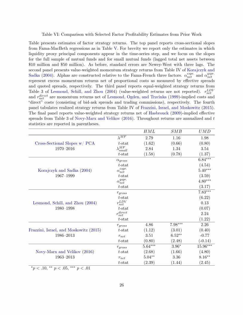
Table VI: Comparison with Selected Factor Profitability Estimates from Prior Work
Table presents estimates of factor strategy returns. The top panel reports cross-sectional slopesfrom Fama-MacBeth regressions as in Table V. For brevity we report only the estimates in whichliquidity proxy principal components appear in the time-series step, and we focus on the slopesfor the full sample of mutual funds and for small mutual funds (lagged total net assets between$10 million and $50 million). As before, standard errors are Newey-West with three lags. Thesecond panel presents value-weighted momentum strategy returns from Table IV of Korajczyk andSadka (2004). Alphas are constructed relative to the Fama-French three factors. ↵espr.
net and ↵qspr.net
represent excess momentum returns net of proportional costs as measured by effective spreadsand quoted spreads, respectively. The third panel reports equal-weighted strategy returns fromTable 3 of Lesmond, Schill, and Zhou (2004) (value-weighted returns are not reported). rLDV
net
and rdirectnet are momentum returns net of Lesmond, Ogden, and Trzcinka (1999)-implied costs and“direct” costs (consisting of bid-ask spreads and trading commissions), respectively. The fourthpanel tabulates realized strategy returns from Table IV of Frazzini, Israel, and Moskowitz (2015).The final panel reports value-weighted strategy returns net of Hasbrouck (2009)-implied effectivespreads from Table 3 of Novy-Marx and Velikov (2016). Throughout returns are annualized and tstatistics are reported in parentheses.
HML SMB UMD
�MF 2.79 1.16 1.98Cross-Sectional Slopes w/ PCA t-stat (1.62) (0.66) (0.80)
1970–2016 �MFsmall 2.84 1.34 3.54t-stat (1.58) (0.78) (1.37)↵gross 6.84⇤⇤⇤t-stat (4.54)
Korajczyk and Sadka (2004) ↵espr.net 5.40⇤⇤⇤
1967–1999 t-stat (3.59)↵qspr.net 4.80⇤⇤⇤t-stat (3.17)rgross 7.83⇤⇤⇤t-stat (6.22)
Lesmond, Schill, and Zhou (2004) rLDVnet 0.13
1980–1998 t-stat (0.07)rdirectnet 2.24t-stat (1.22)rgross 4.86 7.98⇤⇤⇤ 2.26
Frazzini, Israel, and Moskowitz (2015) t-stat (1.12) (3.01) (0.40)1986–2013 rnet 3.51 6.52⇤⇤ -0.77
t-stat (0.80) (2.48) (-0.14)rgross 5.64⇤⇤⇤ 3.96⇤ 15.96⇤⇤⇤
Novy-Marx and Velikov (2016) t-stat (2.68) (1.66) (4.80)1963–2013 rnet 5.04⇤⇤ 3.36 8.16⇤⇤
t-stat (2.39) (1.44) (2.45)⇤p < .10, ⇤⇤ p < .05, ⇤⇤⇤ p < .01
26

(2015) is an outlier, or that non-mutual fund asset managers have different compensation schedulesfor factor exposure.
B. Implementation Costs Over Time
Figure II adds a time-series dimension to the average risk price differences of Tables II–A.I.27
For each panel we plot the log return of the “on-paper” investments in each factor with a unit riskloading minus the corresponding log return on mutual fund investments. To do this we invokethe interpretation of Fama-MacBeth coefficients �kt as the date t return on a portfolio with a unitloading on factor k and zero loading on all other factors. Our series is the centered rolling differencein performance,
yk (t) =t+6X
s=t�6
log�1 + �S
kt
�� log
�1 + �MF
kt
�⇡
t+6X
s=t�6
��kt. (9)
This quantity has an equivalent interpretation as the relative cost associated with real-world ratherthan on-paper investment in factor strategies.
The four panels of Figure II depict factor implementation costs for each set of liquidity proxiesusing the 269 stock portfolios as the on-paper return benchmark. Although magnitudes varyslightly across specifications, the three slope series are remarkably similar for each factor. Theimplementation gap is clearly rank-ordered as UMD, HML, MKT , and SMB, with large andpositive implementation gaps for UMD and HML, no implementation gap for MKT , and a smallnegative implementation gap for SMB. The difference series are also affected by macroeconomicevents. All four implementation gaps fall before the end of the tech bubble of the late 1990s and riseduring the subsequent crash and/or the Great Recession of 2007–2009. One interpretation of thisfeature is that factor returns are most accessible by investment managers when market liquidity isabundant and funding constraints are unlikely to be binding.
Perhaps the most intriguing feature of Figure II is the absence of a trend in strategy implemen-tation costs. This feature contrasts with well-documented secular declines in bid-ask spreads andcommissions since 1970 (e.g., Jones (2002) and Corwin and Schultz (2012)). An equilibrium per-spective on the size of the asset management sector reveals why we instead obtain a stationary timeseries.28 As trading technology improves and equity intermediation becomes more competitive, thecost of trading the first dollar of a factor strategy declines. Perceived sector-level alphas increasefor factor investors, and aggregate inflows attract new entrants (as in Figure I) or contribute to thegrowth of existing fund managers (as in Berk and Green (2004)). These inflows increase the scale offactor investing, which in turn increases non-proportional transactions costs such as price impact.In equilibrium this process continues until factor alphas fall to zero for the marginal dollar. Con-
27In the interest of brevity we suppress the corresponding plots for the matched pairs analysis.28Augmented Dickey-Fuller tests reject the null of a unit root in implementation costs at the 0.1% significance level
in all series.
27

Figure II: Rolling Performance Difference Between Mutual Funds and Stocks (� = 1)
Figures plot the rolling difference between log Fama-MacBeth cross-sectional slopes for stock port-folios (S) and mutual funds (MF ). Each series yk (t) equals the centered rolling difference
yk (t) =t+6X
s=t�6
log�1 + �S
kt
�� log
�1 + �MF
kt
�,
where �kt are cross-sectional slopes from monthly regressions of excess returns rit on time-seriesbetas �̂ik. Each figure plots differences in slopes for which the time-series regression includes noliquidity proxies and the first principal component for market liquidity proxies and funding liquidityproxies. Stock portfolio slopes are estimated using all 269 portfolios described in Section III. Solidlines depict averages of series means. NBER recessions are in gray.
(a) MKT Costs (b) HML Costs
(c) SMB Costs (d) UMD Costs
28

sequently the average dollar invested in factor strategies may see no reduction in implementationcosts despite improvements in trading technology.
The conjectured equilibrium adjustment mechanism hinges on non-proportional trading costs—omitted by studies such as Novy-Marx and Velikov (2016)—and it rationalizes industry-level de-creasing returns to scale suggested by Pastor and Stambaugh (2012) and documented by Pastor,Stambaugh, and Taylor (2015). It also generates a testable prediction that industry-level inflowsincrease implementation costs of factor strategies.
We analyze this relationship between implementation costs, flows, and illiquidity more formallyby examining relating the cost time series with liquidity and fund flow proxies. We start byconstructing illiquidity proxies as the first principal components of market liquidity proxies and offunding liquidity proxies, as described in Section IV.B. We also construct flow variables to capturecosts associated with fund inflows and outflows. Fund flows are the component of asset growth notexplained by returns,
flowit =TNAit
TNAi,t�1� (1 +Rit) . (10)
We summarize the distribution of flows with its first and second cross-sectional moments—the cross-sectional average fund flow (MFLOW ) and the cross-sectional dispersion in fund flows (DFLOW ).In addition to reflecting returns-to-scale, flow variables are a natural candidate for explainingtrading costs because large flows the mutual fund sector or reshuffling of assets among mutualfunds generates liquidity demands. To enhance interpretability, we normalize all right-hand-sidevariables to have mean zero and standard deviation one.
Table VII reports results from a regression of ��kt on the liquidity and fund flow proxies,
��kt = ↵+ �MFLOWMFLOW + �DFLOWDFLOW + �MLPCML + �FLPCFL + ✏kt. (11)
We report only value-weighted results for the 269 stock portfolios because relations between costsand liquidity proxies are quite similar for value-weighted and equal-weighted stock portfolios andfor 100 and 269 stock portfolios. Likewise to be succinct we report only implementation costs in thebaseline specification and with liquidity proxy principal components in Fama-MacBeth time-seriesregression step.
We draw four lessons from Table VII.29 First, the constant terms are large and positive forHML and UMD, confirming that the time-invariant component of implementation costs fromEquation (4) is large and positive for these factors. Second, focusing on flows, average inflows areassociated with higher implementation costs for value and momentum factors, and cross-sectionaldispersion in flows is weakly associated with lower implementation costs for these factors. We findno or unreliable relations for market and size factors, as is expected because these costs are small
29Low R2s throughout are attributable in large part to the noisiness of differences in monthly factor realizations
for stocks and mutual funds.
29

Tabl
eV
II:L
iqui
dity
,Flo
ws,
and
the
Impl
emen
tati
onG
ap
Tabl
ere
port
ses
tim
ates
ofa
regr
essi
onof
annu
aliz
edim
plem
enta
tion
gaps
�� kton
the
first
prin
cipa
lcom
pone
ntof
fund
ing
liqui
dity
prox
ies
(FL
)an
dm
arke
tliq
uidi
typr
oxie
s(M
L),
asw
ell
asth
ecr
oss-
sect
iona
lav
erag
ean
dst
anda
rdde
viat
ion
offu
ndin
flow
s(M
FLOW
andDFLOW
,res
pect
ivel
y),
�� kt=
↵+�M
FLOWM
FLOW
+�DFLOWDFLOW
+�M
LPCM
L+�FLPCFL+✏ k
t,
whe
rek
inde
xes
the
four
Car
hart
(199
7)fa
ctor
s.Im
plem
enta
tion
cost
sar
ees
tim
ated
wit
hpr
inci
palco
mpo
nent
sof
mar
ket
and
fund
ing
liqui
dity
prox
ies
inth
eti
me-
seri
esre
gres
sion
sfo
rm
utua
lfu
ndan
dst
ock
port
folio
beta
s.Li
quid
itypr
oxie
san
dst
ock
port
folio
sets
are
desc
ribe
din
Sect
ion
III.
Illiq
uidi
typr
inci
palc
ompo
nent
sha
veun
itst
anda
rdde
viat
ion
and
are
cons
truc
ted
tobe
nega
tive
lyco
rrel
ated
wit
hth
em
arke
tret
urn
and
posi
tive
lyco
rrel
ated
wit
hth
eV
IX/V
XO
.Fun
dflo
wsa
reTNA
it/T
NA
i,t�1�(1
+R
it).
Stan
dard
erro
rsar
eN
ewey
-Wes
tw
ith
thre
ela
gs.t
stat
istics
are
repo
rted
inpa
rent
hese
s.(a
)Im
plem
enta
tion
Cos
ts—
Bas
elin
eSp
ecifi
cati
on
MK
TH
ML
SMB
UM
D�M
FLOW
0.02
-0.1
21.
97⇤⇤
0.94
0.56
0.36
2.66
⇤⇤1.
66t-
stat
(0.0
7)(-
0.45
)(2
.43)
(1.0
8)(0
.98)
(0.5
5)(2
.06)
(1.2
3)�DFLOW
-0.0
1-0
.05
-2.2
2⇤⇤
-2.4
8⇤⇤
-0.0
8-0
.17
-2.7
6-2
.99
t-st
at(-
0.01
)(-
0.12
)(-
2.07
)(-
2.35
)(-
0.13
)(-
0.27
)(-
1.43
)(-
1.56
)�M
L0.
420.
442.
53⇤⇤
2.76
⇤⇤⇤
0.98
0.96
2.31
2.52
t-st
at(1
.27)
(1.3
1)(2
.40)
(2.6
7)(1
.14)
(1.0
8)(1
.13)
(1.1
9)�FL
-0.4
2-0
.48
-3.3
5⇤⇤⇤
-3.4
8⇤⇤⇤
-0.9
0-0
.78
-3.4
2⇤-0
.78
t-st
at(-
1.18
)(-
1.26
)(-
3.47
)(-
3.21
)(-
1.04
)(-
0.80
)(-
1.93
)(-
0.80
)↵
-0.2
0-0
.20
-0.2
02.
71⇤⇤
⇤2.
71⇤⇤
⇤2.
71⇤⇤
⇤-0
.49
-0.4
9-0
.49
7.00
⇤⇤⇤
7.00
⇤⇤⇤
7.00
⇤⇤⇤
t-st
at(-
0.80
)(-
0.80
)(-
0.80
)(3
.92)
(3.9
0)(3
.95)
(-0.
83)
(-0.
83)
(-0.
83)
(5.4
6)(5
.42)
(5.5
2)R
20.
000.
010.
010.
020.
040.
060.
000.
000.
010.
010.
010.
02⇤ p
<.10,
⇤⇤p<
.05,
⇤⇤⇤p<
.01
(b)
Impl
emen
tati
onC
osts
—Li
quid
ityP
Cs
MK
TH
ML
SMB
UM
D�M
FLOW
0.05
-0.1
32.
45⇤⇤
⇤1.
130.
510.
353.
80⇤⇤
⇤1.
29t-
stat
(0.2
0)(-
0.50
)(2
.78)
(1.2
2)(0
.91)
(0.5
4)(2
.88)
(0.9
7)�DFLOW
0.02
-0.0
3-1
.95⇤
-2.2
4⇤⇤
-0.2
3-0
.35
-2.3
0-2
.54
t-st
at(0
.05)
(-0.
07)
(-1.
70)
(-2.
01)
(-0.
38)
(-0.
57)
(-1.
19)
(-1.
36)
�M
L0.
470.
493.
00⇤⇤
⇤3.
17⇤⇤
⇤1.
311.
322.
102.
29t-
stat
(1.4
4)(1
.47)
(2.9
5)(3
.25)
(1.4
0)(1
.35)
(1.0
9)(1
.16)
�FL
-0.5
5-0
.62
-4.3
7⇤⇤⇤
-4.3
7⇤⇤⇤
-0.8
4-0
.77
-7.3
6⇤⇤⇤
-0.7
7t-
stat
(-1.
58)
(-1.
63)
(-4.
50)
(-4.
09)
(-0.
96)
(-0.
78)
(-4.
44)
(-0.
78)
↵-0
.21
-0.2
1-0
.21
2.99
⇤⇤⇤
2.99
⇤⇤⇤
2.99
⇤⇤⇤
-0.4
5-0
.45
-0.4
57.
15⇤⇤
⇤7.
15⇤⇤
⇤7.
15⇤⇤
⇤
t-st
at(-
0.83
)(-
0.83
)(-
0.83
)(4
.10)
(4.1
6)(4
.21)
(-0.
76)
(-0.
77)
(-0.
77)
(5.5
6)(5
.73)
(5.8
2)R
20.
000.
010.
010.
020.
060.
070.
000.
010.
010.
010.
050.
06⇤ p
<.10,
⇤⇤p<
.05,
⇤⇤⇤p<
.01
30

in magnitude to begin with. We interpret these relations as suggestive evidence that (1) inflows areexpensive from a transactions-cost standpoint for funds trading value and momentum strategies,thereby contributing to diseconomies of scale and stationary average implementation costs, and (2)reallocation of funds within the mutual fund sector may increase other-funds’ liquidity trading (ina Kyle (1985) sense), thereby reducing transactions costs for value and momentum traders. Third,focusing on illiquidity principal components, market illiquidity increases implementation costs, andparticularly so for value and momentum strategies. Intuitively trading becomes more expensivewhen market liquidity is low. Fourth, funding illiquidity conversely decreases implementation costs(again most strongly for HML and UMD). We conjecture that mutual funds are insulated fromfunding liquidity shocks that affect more highly levered institutional asset managers like hedge funds(Sadka (2010) and Boyson, Stahel, and Stulz (2010), among others, discuss hedge funds’ particularvulnerability to funding liquidity shocks), and hence mutual funds can acquire the ingredients offactor strategies from distressed asset managers at a discount during times of strained fundingliquidity.
VII. Robustness Tests
A. Are Costs Asymmetric for Long- and Short-Factor Strategies?
The implementation gap �� reflects the difference between on-paper and real-world perfor-mance for a factor strategy. For positive-beta funds, this difference has a clear interpretation asimplementation shortfall, but this interpretation is strained for negative-beta funds. For example apositive �� for HML suggests that funds with negative value-factor exposure outperform on-paperinvestments in growth stocks. Positive ��
HML and ��UMD estimates therefore may signal better-
than-expected performance in growth and contrarian strategies rather than large implementationcosts in value and momentum strategies. The prevalence of dedicated “growth” mutual funds givescredence to this alternative interpretation and motivates our examination of implementation costsseparately for funds with positive and negative factor exposures.
We adapt our Fama-MacBeth approach to accommodate different cross-sectional compensationfor positive and negative factor exposures as follows. The time-series regression step of Equation (1)remains the same as before, whereas we adapt the cross-sectional step of Equation (2) to bifurcaterisk compensation into slopes among positive-beta and negative-beta funds and stock portfolios:
rit =X
k
⇣�S,+kt 1�̂ik>0 + �S,�
kt 1�̂ik<0
⌘�̂ik1i2S
+X
k
⇣�MF,+kt 1�̂ik>0 + �MF,�
kt 1�̂ik<0
⌘�̂ik1i2MF + ✏it, t = 1, . . . , T. (12)
The differences ��,+ ⌘ �S,+ � �MF,+ and ��,� ⌘ �S,� � �MF,� reflect implementation gaps for
31

going long a factor and implementation gains for going short a factor, respectively. In estimatingEquation (12) we drop the negative-beta terms for the market factor because 99% of our mutualfunds and 100% of our stock portfolios have positive four-factor market betas.
Table VIII reports the results of this decomposition without liquidity proxies (results are similarfor principal component specifications in which these proxies are included). The first four columnsassess the implementability of factor strategies and are our focus. Here we obtain coefficients muchlike those of Table II with two important differences. First, while the costs of implementing value��,+HML are comparable in magnitude to those of Table II, the point estimate �MF
HML is about 50%larger in our split specification—4.2% versus 2.8% in the long sample and 3.2% versus 2.2% inthe recent sample. Conversely, the implementation costs for momentum ��,+
UMD increase from 7%to 11%–12% in the long sample and from 5% to 10%–11% in the recent sample to completelyeliminate returns to the momentum anomaly (�MF,+
UMD ⇡ 0). We conclude that outperformance innegative-beta strategies does not drive the low estimated compensation to value and momentumexposure.
We obtain mixed results for implementation costs of short-factor strategies with negative on-paper expected excess returns. For mutual funds we estimate only a 1.6% decline in averagereturns associated with decreasing �HML one unit further below zero, whereas we see a declineof 2.5%–5.6% in average returns for stock portfolios. Mutual funds thus slightly outperform on-paper growth strategies. Conversely, mutual funds implement large-cap strategies relatively poorly,with large negative ��,� on the order of 5%–9%. In both cases we hesitate to draw conclusionsbased on these estimates because few stock portfolios have negative multifactor value betas; thecross-sectional regression coefficients are likely to be poorly identified, and indeed, coefficients varysubstantially between 100-portfolio and 269-portfolio specifications.
By contrast, roughly half of our stock portfolios and mutual funds have negative momentumbetas. In this better-identified setting, we find no implementation costs (or gains) associated withshorting momentum. A one-unit decline in momentum factor exposure translates into sharply loweraverage returns for both real-world and on-paper portfolios. In conjunction with our positive-�UMD
results, mutual funds reap none of the upside of exploiting momentum and all of the downside ofbeing contrarian. This rather bleak result for typical mutual funds differs from the high premiumto momentum exposure in stock portfolios on both the long and short side, as Israel and Moskowitz(2013) also find.
B. Do Omitted Strategies Explain High Measured Costs?
Omitted mutual fund strategies may bias our implementation cost estimates. Bias occurs ifincidental factor exposures incurred by other activities are cross-sectionally correlated with mutualfund returns. However, the potential for meaningful contamination of cross-sectional slopes de-creases with the power of the Carhart (1997) model for explaining time-series variation in returns.
32

Table VIII: Implementation Cost Estimates in Fama-MacBeth Regressions — Asymmetric Costs
Table reports Fama-MacBeth estimates of the compensation for factor exposure for positive andnegative beta stock portfolios (second panel), domestic equity mutual funds (third panel), andtheir difference (top panel). Coefficients are the average cross-sectional slopes �̄k across monthlyregressions of excess returns rit on time-series betas �̂ik,
rit =X
k
⇣�S,+kt 1�̂ik>0 + �S,�
kt 1�̂ik<0
⌘�̂ik1i2S+
X
k
⇣�MF,+kt 1�̂ik>0 + �MF,�
kt 1�̂ik<0
⌘�̂ik1i2MF+✏it, t = 1, . . . , T,
where k indexes the four Carhart (1997) factors and �� is defined as �S ��MF . %�k rows indicatethe percentage of four-factor betas that are positive (left columns) or negative (right columns).Because betas are universally positive on the market factor we drop its associated negative-betaterms. Stock portfolio sets are described in Section III. All coefficients are annualized and reportedin percent. Standard errors are Newey-West with three lags. t statistics are reported in parentheses.
(a) Value-Weighted Stock Portfolios (1970 – 2016)
Positive �k Negative �kNS MKT HML SMB UMD HML SMB UMD
�� 100 -1.08⇤ 3.54⇤⇤⇤ 0.35 12.81⇤⇤⇤ 4.00⇤⇤⇤ -5.36⇤ 1.06t-stat (-1.71) (3.43) (0.37) (6.46) (2.99) (-1.91) (0.61)
�� 269 -1.25⇤⇤⇤ 2.57⇤⇤⇤ 0.55 11.39⇤⇤⇤ 0.86 -8.98⇤⇤⇤ 1.20t-stat (-3.16) (2.81) (0.76) (6.38) (0.64) (-4.32) (0.72)
�S 100 6.12⇤⇤ 7.76⇤⇤⇤ 1.03 12.37⇤⇤⇤ 5.60⇤⇤⇤ 0.30 8.06⇤⇤⇤t-stat (2.49) (4.05) (0.56) (4.61) (2.66) (0.09) (3.25)
%�Sk 100 86 82 42 14 18 58
�S 269 5.95⇤⇤ 6.80⇤⇤⇤ 1.24 10.95⇤⇤⇤ 2.46 -3.32 8.20⇤⇤⇤t-stat (2.46) (3.70) (0.72) (4.16) (1.07) (-1.13) (3.39)
%�Sk 100 83 73 38 17 27 62
�MF — 7.20⇤⇤⇤ 4.22⇤⇤ 0.68 -0.44 1.60 5.66⇤⇤ 7.00⇤⇤t-stat (2.98) (2.44) (0.39) (-0.17) (0.84) (2.26) (2.47)
%�MFk 99 56 60 48 44 40 52
T 564 564 564 564 564 564 564N̄MF 1901 1901 1901 1901 1901 1901 1901⇤p < .10, ⇤⇤ p < .05, ⇤⇤⇤ p < .01
(b) Value-Weighted Stock Portfolios (1993 – 2016)
Positive �k Negative �kNS MKT HML SMB UMD HML SMB UMD
�� 100 -1.12 3.28⇤⇤⇤ 0.32 11.37⇤⇤⇤ 4.71⇤⇤ -4.28 -0.64t-stat (-1.40) (3.05) (0.24) (3.95) (2.49) (-1.13) (-0.31)
�� 269 -1.23⇤⇤ 2.76⇤⇤⇤ 0.19 10.09⇤⇤⇤ -0.43 -9.25⇤⇤⇤ 0.18t-stat (-2.47) (3.15) (0.20) (3.89) (-0.36) (-3.42) (0.09)
�S 100 6.88⇤⇤ 6.48⇤⇤ 2.21 8.96⇤⇤ 5.95⇤ -0.39 5.08t-stat (2.09) (2.21) (0.84) (2.09) (1.87) (-0.08) (1.33)
%�Sk 100 82 80 40 18 20 60
�S 269 6.77⇤⇤ 5.96⇤⇤ 2.08 7.69⇤ 0.81 -5.37 5.89t-stat (2.07) (2.03) (0.85) (1.88) (0.27) (-1.23) (1.55)
%�Sk 100 82 71 39 18 29 61
�MF — 8.00⇤⇤ 3.20 1.89 -2.40 1.24 3.88 5.72t-stat (2.48) (1.22) (0.80) (-0.62) (0.41) (1.27) (1.33)
%�MFk 99 57 57 47 43 43 53
T 282 282 282 282 282 282 282N̄MF 3299 3299 3299 3299 3299 3299 3299⇤p < .10, ⇤⇤ p < .05, ⇤⇤⇤ p < .01
33
For especially high R2 values in the time-series regressions, the scope for omitted variable bias issmall if coefficients are stable across specifications, as they are in our study (Oster (2017)).
We split our sample into R2 quintiles to bound potential bias arising from omitted fund strate-gies. To perform this split, we run the time-series regressions fund-by-fund as before using theCarhart (1997) model, and we sort funds into one of five equally-spaced bins at each date based onthe R2 of its time-series regression. Funds with high R2 have returns nearly spanned by one or moreacademic strategies, and these funds have little scope for omitted strategies that might complicatethe interpretations of �MF and ��. Conversely funds with lower R2 either (1) implement academicstrategies with greater discretion and/or tracking error or (2) implement strategies that we cannotobserve. We then construct cross-sectional mutual fund factor compensation estimates for each R2
group as in Tables II–A.I.Table IX presents results from the splits by explanatory power of the four-factor model on the
full 1970–2016 sample. The decomposition by R2 delivers two results related to omitted strategies.First, funds with the highest R2s achieve similar performance on the market factor to the typicalmutual fund, and somewhat higher performance on all non-market factors. These differences arenot statistically distinguishable, however, nor is performance statistically distinguishable acrossany set of segmented funds for any factor and first-stage specification. Second, even the fundsthat most closely track the four academic factors continue to significantly underperform the on-paper factors. Value premia are more than 1% larger among the funds most closely mimickingacademic factors, and compensation for value exposure is significantly different from zero at the5% level for R2 quintiles four and five. Even so, the best-performing R2 segments for value stillsee an implementation gap of 1%–2% relative to the stock portfolios. Returns to momentumexposure for the highest R2 group are nearly double those of the typical mutual fund, but theyare not statistically significant in any specification, and the implementation gap for these funds��5 ⌘ �S � �MF
5 is different from zero at the 1% level. Taken together these findings suggest thatour results are not explained by an omitted strategies bias.
Table IX also adds color to how funds implement asset pricing factors. For the market factor,funds with greater deviations from the academic factors typically achieve greater returns to marketbeta. Small deviations from the CRSP market go a long way toward reducing implementationcosts for the aggregate market: the market factor is compensated 20–88 basis points more inmutual funds that track the four factors less well. This finding reinforces the importance of usingomnibus approaches to measuring implementation costs that are robust to real-world departuresfrom the academic factors. Finally, for the non-market factors, strategy deviations from the fourfactors decrease factor compensation, sometimes substantially. Funds that take on factor risk whilepursuing non-factor strategies are rarely compensated well for that risk: destroying returns relativeto an index strategy is common.
34

Tabl
eIX
:Fam
a-M
acB
eth
Slop
esfo
rSt
ocks
and
Mut
ualF
unds
—R
2Q
uint
ileSp
lits
Tabl
ere
port
sFa
ma-
Mac
Bet
hes
tim
ates
ofth
eco
mpe
nsat
ion
for
fact
orex
posu
refo
rdo
mes
tic
equi
tym
utua
lfu
nds.
Coe
ffici
ents
are
the
aver
age
cros
s-se
ctio
nals
lope
s�̄g k
acro
ssm
onth
lyre
gres
sion
sof
exce
ssre
turn
sr iton
tim
e-se
ries
beta
s�̂ik
for
each
grou
pof
mut
ualf
unds
g,r it=X k
�M
F,g
kt
�̂ik+✏ it,
t=
1,...,T,g=
1,...,5,
whe
rek
inde
xes
the
four
Car
hart
(199
7)fa
ctor
s.W
epa
rtit
ion
mut
ualf
unds
into
five
equa
lgro
ups
sort
edby
tim
e-se
ries
regr
essi
onR
2s
from
the
Car
hart
mod
el,w
here
R2
cuto
ffsar
ese
tat
each
date
base
don
the
sam
ple
ofliv
efu
nds.
“5”
indi
cate
sth
ehi
ghes
tR
2
fund
s,an
d“1
”in
dica
testh
elo
wes
tR2
fund
s.T
hefir
stco
lum
nre
port
sth
eav
erag
eR
2sac
ross
allf
und-
date
obse
rvat
ions
wit
hin
each
R2
grou
p.Su
bseq
uent
first
-sta
gere
gres
sion
esti
mat
esin
clud
eth
ese
fact
ors
only
(firs
tco
lum
ns)
and
the
first
prin
cipa
lcom
pone
ntof
mar
ket
and
fund
ing
liqui
dity
prox
ies
(sec
ond
colu
mns
).Li
quid
itypr
oxie
san
dst
ock
port
folio
sets
are
desc
ribe
din
Sect
ion
III.
�� 5
isth
edi
ffere
nce
betw
een
com
pens
atio
nfo
rfa
ctor
expo
sure
betw
een
the
269
stoc
kpo
rtfo
lios
and
the
high
estR
2fu
ndgr
oup.
All
coeffi
cien
tsar
ean
nual
ized
and
repo
rted
inpe
rcen
t.St
anda
rder
rors
are
New
ey-W
est
wit
hth
ree
lags
.t
stat
istics
are
repo
rted
inpa
rent
hese
s.T
hefin
alth
ree
row
sre
port
thep
valu
esof
test
sof
coeffi
cien
tsbe
ing
join
tly
diffe
rent
from
zero
,of
equa
lity
ofco
effici
ents
,and
ofno
n-m
onot
onic
ityof
coeffi
cien
ts(u
sing
the
test
ofPa
tton
and
Tim
mer
man
n(2
010)
).
No
Liq
uid
ity
Proxie
sLiq
uid
ity
PC
s
R̄2
MKT
HM
LSM
BUM
DM
KT
HM
LSM
BUM
D
�M
F5
94.6
%6.
55⇤⇤
⇤3.
78⇤⇤
2.13
3.88
6.55
⇤⇤⇤
4.00
⇤⇤2.
034.
20t-
stat
(2.7
2)(2
.11)
(1.2
4)(1
.43)
(2.7
3)(2
.21)
(1.1
8)(1
.57)
�M
F4
90.7
%6.
75⇤⇤
⇤4.
04⇤⇤
2.77
⇤2.
526.
71⇤⇤
⇤4.
29⇤⇤
2.83
⇤2.
54t-
stat
(2.7
7)(2
.19)
(1.6
5)(0
.92)
(2.7
6)(2
.28)
(1.6
9)(0
.92)
�M
F3
87.1
%7.
43⇤⇤
⇤2.
48-0
.21
3.22
7.41
⇤⇤⇤
2.48
-0.1
32.
68t-
stat
(3.0
1)(1
.43)
(-0.
12)
(1.2
3)(3
.00)
(1.4
0)(-
0.08
)(1
.04)
�M
F2
82.1
%7.
20⇤⇤
⇤2.
511.
870.
467.
16⇤⇤
⇤2.
391.
86-0
.08
t-st
at(2
.94)
(1.4
7)(1
.08)
(0.1
8)(2
.93)
(1.3
6)(1
.07)
(-0.
03)
�M
F1
60.0
%7.
09⇤⇤
⇤3.
10-0
.59
2.40
7.25
⇤⇤⇤
3.36
⇤-1
.13
2.58
t-st
at(2
.87)
(1.6
3)(-
0.27
)(0
.81)
(2.9
4)(1
.76)
(-0.
51)
(0.8
8)�� 5
–0.
231.
68⇤⇤
-1.3
6⇤⇤
5.26
⇤⇤⇤
0.23
1.77
⇤⇤-1
.32⇤
⇤4.
92⇤⇤
⇤
t-st
at(0
.99)
(2.0
7)(-
2.28
)(3
.49)
(0.9
6)(2
.13)
(-2.
20)
(3.1
3)�M
F82
.9%
6.98
⇤⇤⇤
2.75
1.25
2.14
6.98
⇤⇤⇤
2.79
1.16
1.98
t-st
at(2
.87)
(1.6
1)(0
.71)
(0.8
6)(2
.88)
(1.6
2)(0
.66)
(0.8
0)�=
00.
00⇤⇤
⇤0.
00⇤⇤
⇤0.
380.
380.
00⇤⇤
⇤0.
00⇤⇤
⇤0.
350.
37�=
1.00
0.94
0.57
0.92
1.00
0.90
0.47
0.85
��◆◆70
0.51
0.21
0.98
0.40
0.51
0.38
0.98
0.60
⇤ p<
.10,
⇤⇤p<
.05,
⇤⇤⇤p<
.01
35
C. Do Microcap Stocks Explain Superior On-Paper Performance?
Implementation frictions attenuate the returns to traded securities and motivate investors todepart from prescribed factor strategies. Frictions that reduce the set of investment opportunitiesare an important “shadow” implementation cost—analogous to the shadow price on a constraint onwhich stocks can be included in a portfolio—faced by real-world investors and missed by existingmeasures of costs. In this section we consider the role of security size in circumscribing mutualfunds’ investable universe. Security size is a natural candidate for explaining the performance gapbetween on-paper and real-world factor investing because (1) the highest returns to HML exposureare earned in the smallest stocks (Fama and French (2012), Israel and Moskowitz (2013)), and (2)low market capitalization securities are too small to accommodate the capital of large mutual funds.
The smallest stocks or “microcaps” present especially challenging environments for asset man-agers because of their particularly low carrying capacities and high transaction costs. Perhapsbecause of the challenges facing potential arbitrageurs in this space, the majority of academicanomalies only exist in these “dusty corners” of the stock market (Hou, Xue, and Zhang (2017)).To evaluate the effect of microcaps on our cost estimates, we exclude microcaps from our set ofstock portfolios. We follow Fama and French (2008) and Hou, Xue, and Zhang (2017) in definingmicrocaps as stocks with market capitalization less than the 20th percentile of NYSE market capi-talization, and we implement this filter by dropping the smallest-size portfolios from double-sortedsize-value, size-beta, size-prior return, and size-Amihud portfolios. This exclusion eliminates a fifthof the portfolios but only 3% of market capitalization (Fama and French (2008)).
Table X reports Fama-MacBeth estimates of factor premia on this set of stock portfolios. Wepresent only value-weighted results because we are interested in shaping our stock portfolios toreflect the investible universe. Our main finding is that microcaps indeed explain some of themeasured performance attrition for value and momentum strategies, but not enough to close themeasured implementation gap. As a useful placebo, the gap on replicating performance on thevalue-weighted market changes by at most a few basis points.
In the 1970–2016 sample, both value and momentum compensation are about 1% smaller inthe stock portfolios in which microcaps are excluded. This difference persists for value in the morerecent sample, echoing Fama and French (2012) and Israel and Moskowitz (2013), but it roughlyhalves for momentum. Nevertheless, the performance gap between sans-microcap stock portfoliosand mutual funds remains economically large and statistically robust. If mutual funds indeed cannotinvest in microcap stocks, this narrowing of the investible universe explains (at most) 23%–27% ofthe implementation gap for value and 17%–18% of the implementation gap for momentum.
36
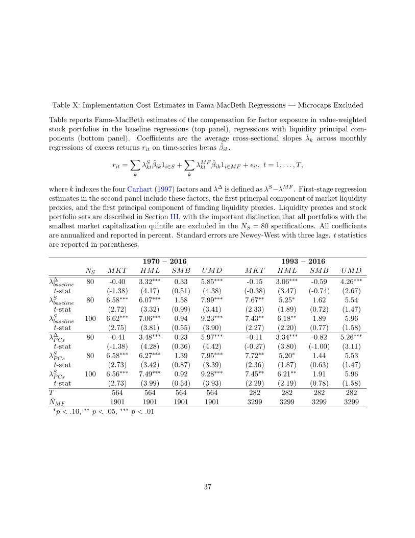
Table X: Implementation Cost Estimates in Fama-MacBeth Regressions — Microcaps Excluded
Table reports Fama-MacBeth estimates of the compensation for factor exposure in value-weightedstock portfolios in the baseline regressions (top panel), regressions with liquidity principal com-ponents (bottom panel). Coefficients are the average cross-sectional slopes �̄k across monthlyregressions of excess returns rit on time-series betas �̂ik,
rit =X
k
�Skt�̂ik1i2S +
X
k
�MFkt �̂ik1i2MF + ✏it, t = 1, . . . , T,
where k indexes the four Carhart (1997) factors and �� is defined as �S��MF . First-stage regressionestimates in the second panel include these factors, the first principal component of market liquidityproxies, and the first principal component of funding liquidity proxies. Liquidity proxies and stockportfolio sets are described in Section III, with the important distinction that all portfolios with thesmallest market capitalization quintile are excluded in the NS = 80 specifications. All coefficientsare annualized and reported in percent. Standard errors are Newey-West with three lags. t statisticsare reported in parentheses.
1970 – 2016 1993 – 2016
NS MKT HML SMB UMD MKT HML SMB UMD
��baseline 80 -0.40 3.32⇤⇤⇤ 0.33 5.85⇤⇤⇤ -0.15 3.06⇤⇤⇤ -0.59 4.26⇤⇤⇤t-stat (-1.38) (4.17) (0.51) (4.38) (-0.38) (3.47) (-0.74) (2.67)
�Sbaseline 80 6.58⇤⇤⇤ 6.07⇤⇤⇤ 1.58 7.99⇤⇤⇤ 7.67⇤⇤ 5.25⇤ 1.62 5.54t-stat (2.72) (3.32) (0.99) (3.41) (2.33) (1.89) (0.72) (1.47)
�Sbaseline 100 6.62⇤⇤⇤ 7.06⇤⇤⇤ 0.94 9.23⇤⇤⇤ 7.43⇤⇤ 6.18⇤⇤ 1.89 5.96t-stat (2.75) (3.81) (0.55) (3.90) (2.27) (2.20) (0.77) (1.58)
��PCs 80 -0.41 3.48⇤⇤⇤ 0.23 5.97⇤⇤⇤ -0.11 3.34⇤⇤⇤ -0.82 5.26⇤⇤⇤t-stat (-1.38) (4.28) (0.36) (4.42) (-0.27) (3.80) (-1.00) (3.11)
�SPCs 80 6.58⇤⇤⇤ 6.27⇤⇤⇤ 1.39 7.95⇤⇤⇤ 7.72⇤⇤ 5.20⇤ 1.44 5.53t-stat (2.73) (3.42) (0.87) (3.39) (2.36) (1.87) (0.63) (1.47)
�SPCs 100 6.56⇤⇤⇤ 7.49⇤⇤⇤ 0.92 9.28⇤⇤⇤ 7.45⇤⇤ 6.21⇤⇤ 1.91 5.96t-stat (2.73) (3.99) (0.54) (3.93) (2.29) (2.19) (0.78) (1.58)
T 564 564 564 564 282 282 282 282N̄MF 1901 1901 1901 1901 3299 3299 3299 3299⇤p < .10, ⇤⇤ p < .05, ⇤⇤⇤ p < .01
37

VIII. Conclusion
Existing methods for assessing the implementation costs of financial market anomalies useproprietary trading data for single firms or market-wide trading data combined with parametrictransactions cost models. We propose two new methods (an extension of the Fama-MacBethapproach, and a matched pairs approach) to estimate implementation costs using only returns datafrom stocks and mutual funds. Doing so frees us from the requirement of specifying factor tradingstrategies and transaction costs models that may be incomplete or misspecified. Moreover, the readyavailability of returns data for a large number of investment managers enables the examination offactor implementation costs for a large investment management universe.
Both of our proposed approaches demonstrate that mutual funds are generally poorly compen-sated for exposure to common risk factors. Our estimates based on Fama-MacBeth regressionsimply that implementation costs erode almost the entirety of the return to value and momentumstrategies for typical mutual funds, but have little effect on market and size factor strategies. Ourestimates based on matched pairs suggest comparable performance attrition for value and momen-tum strategies, and they differ in revealing high costs to investing in small-stock characteristicportfolios.
Taken together, these results paint a sobering picture of the real-world returns to the mostimportant financial market anomalies. We agree with Lesmond, Schill, and Zhou (2004)’s analysisthat momentum profits in particular may be out of reach for the typical asset manager. In thisrespect markets may be efficient from the perspective of representative mutual funds, even if outlierfunds see a very different picture of risk and return net-of-costs (e.g., the asset manager of Frazzini,Israel, and Moskowitz (2015)).
Our approaches are readily extended to a wide range of candidate return factors provided thatthese are reflected in mutual fund exposures. Common anomalies like size, value, and momen-tum clearly meet this requirement. In future research we will apply these tools more broadly toinvestigate whether other inhabitants of the factor zoo truly can survive in the wild.
38
References
Abadie, Alberto and Guido W. Imbens. 2006. “Large Sample Properties of Matching Estimatorsfor Average Treatment Effects.” Econometrica 74 (1):235–267.
———. 2011. “Bias-Corrected Matching Estimators for Average Treatment Effects.” Journal ofBusiness & Economic Statistics 29 (1):1–11.
Amihud, Yakov. 2002. “Illiquidity and Stock Returns: Cross-Section and Time-Series Effects.”Journal of Financial Markets 5 (1):31 – 56.
Arnott, Robert D., Vitali Kalesnik, and Lillian J. Wu. 2017. “The Incredible Shrinking FactorReturn.” Working paper.
Asness, Clifford S., Tobias J. Moskowitz, and Lasse Heje Pedersen. 2013. “Value and MomentumEverywhere.” The Journal of Finance 68 (3):929–985.
Banz, Rolf W. 1981. “The Relationship Between Return and Market Value of Common Stocks.”Journal of Financial Economics 9 (1):3 – 18.
Barroso, Pedro and Pedro Santa-Clara. 2015. “Momentum Has Its Moments.” Journal of FinancialEconomics 116 (1):111 – 120.
Basu, S. 1977. “Investment Performance of Common Stocks in Relation to Their Price-EarningsRatios: A Test of the Efficient Market Hypothesis.” The Journal of Finance 32 (3):663–682.
Berk, Jonathan B. and Richard C. Green. 2004. “Mutual Fund Flows and Performance in RationalMarkets.” Journal of Political Economy 112 (6):1269–1295.
Berk, Jonathan B. and Jules H. van Binsbergen. 2015. “Measuring Skill in the Mutual FundIndustry.” Journal of Financial Economics 118 (1):1 – 20.
Boyson, Nicole M., Christof W. Stahel, and René M. Stulz. 2010. “Hedge Fund Contagion andLiquidity Shocks.” The Journal of Finance 65 (5):1789–1816.
Breen, William J., Laurie Simon Hodrick, and Robert A. Korajczyk. 2002. “Predicting EquityLiquidity.” Management Science 48 (4):470–483.
Brunnermeier, Markus K. 2009. “Deciphering the Liquidity and Credit Crunch 2007–2008.” TheJournal of Economic Perspectives 23 (1):77–100.
Bühlmann, Peter and S. van de Geer. 2011. Statistics for High-Dimensional Data: Methods, Theory,and Applications. Springer Series in Statistics.
39
Carhart, Mark M. 1997. “On Persistence in Mutual Fund Performance.” The Journal of Finance52 (1):57–82.
Chen, Zhiwu, Werner Stanzl, and Masahiro Watanabe. 2002. “Price Impact Costs and the Limitof Arbitrage.” Working paper.
Chetverikov, Denis, Zhipeng Liao, and Victor Chernozhukov. 2017. “On Cross-Validated Lasso.”Working paper.
Cochrane, John H. 2011. “Presidential Address: Discount Rates.” The Journal of Finance66 (4):1047–1108.
Corwin, Shane A. and P. Schultz. 2012. “A Simple Way to Estimate Bid-Ask Spreads from DailyHigh and Low Prices.” The Journal of Finance 67 (2):719–760.
Daniel, Kent, Mark Grinblatt, Sheridan Titman, and Russ Wermers. 1997. “Measuring Mutual FundPerformance with Characteristic-Based Benchmarks.” The Journal of Finance 52 (3):1035–1058.
Elton, Edwin J., Martin J. Gruber, and Christopher R. Blake. 2001. “A First Look at the Accuracyof the CRSP Mutual Fund Database and a Comparison of the CRSP and Morningstar MutualFund Databases.” The Journal of Finance 56 (6):2415–2430.
Engle, Robert, Robert Ferstenberg, and Jeffrey Russell. 2012. “Measuring and Modeling ExecutionCost and Risk.” The Journal of Portfolio Management 38 (2):14–28.
Fama, Eugene F. 1970. “Efficient Capital Markets: A Review of Theory and Empirical Work.” TheJournal of Finance 25 (2):383–417.
Fama, Eugene F. and K. R. French. 2010. “Luck Versus Skill in the Cross-Section of Mutual FundReturns.” The Journal of Finance 65 (5):1915–1947.
Fama, Eugene F. and Kenneth R. French. 1992. “The Cross-Section of Expected Stock Returns.”Journal of Finance 47 (2):427–465.
———. 2008. “Dissecting Anomalies.” The Journal of Finance 63 (4):1653–1678.
———. 2012. “Size, Value, and Momentum in International Stock Returns.” Journal of FinancialEconomics 105 (3):457 – 472.
Fama, Eugene F. and James D. MacBeth. 1973. “Risk, Return, and Equilibrium: Empirical Tests.”Journal of Political Economy 81 (3):607–636.
Frazzini, Andrea, Ronen Israel, and Tobias J. Moskowitz. 2015. “Trading Costs of Asset PricingAnomalies.” Working paper.
40

Frazzini, Andrea and Lasse Heje Pedersen. 2014. “Betting Against Beta.” Journal of FinancialEconomics 111 (1):1 – 25.
Giglio, Stefano and Dacheng Xiu. 2017. “Inference on Risk Premia in the Presence of OmittedFactors.” Working paper.
Glosten, Lawrence R and Lawrence E Harris. 1988. “Estimating the Components of the Bid/AskSpread.” Journal of Financial Economics 21 (1):123 – 142.
Grinblatt, Mark, Sheridan Titman, and Russ Wermers. 1995. “Momentum Investment Strategies,Portfolio Performance, and Herding: A Study of Mutual Fund Behavior.” The American Eco-nomic Review 85 (5):1088–1105.
Grundy, Bruce D. and J. Spencer Martin. 2001. “Understanding the Nature of the Risks and theSource of the Rewards to Momentum Investing.” The Review of Financial Studies 14 (1):29–78.
Harvey, Campbell R. 2017. “Presidential Address: The Scientific Outlook in Financial Economics.”The Journal of Finance 72 (4):1399–1440.
Harvey, Campbell R., Yan Liu, and Heqing Zhu. 2016. “... and the Cross-Section of ExpectedReturns.” The Review of Financial Studies 29 (1):5–68.
Hasbrouck, Joel. 2009. “Trading Costs and Returns for U.S. Equities: Estimating Effective Costsfrom Daily Data.” The Journal of Finance 64 (3):1445–1477.
Hastie, T., R. Tibshirani, and M. Wainwright. 2015. Statistical Learning with Sparsity: The Lassoand Generalizations. CRC Press.
He, Zhiguo, Bryan Kelly, and Asaf Manela. 2017. “Intermediary Asset Pricing: New Evidence fromMany Asset Classes.” Journal of Financial Economics .
Hou, Kewei, Chen Xue, and Lu Zhang. 2017. “Replicating Anomalies.” Working paper.
Imbens, Guido W. and Donald B. Rubin. 2015. Causal Inference for Statistics, Social, and Biomed-ical Sciences: An Introduction. Cambridge University Press, 1st ed. ed.
Israel, Ronen and Tobias J. Moskowitz. 2013. “The Role of Shorting, Firm Size, and Time onMarket anomalies.” Journal of Financial Economics 108 (2):275 – 301.
Jegadeesh, Narasimhan and Sheridan Titman. 1993. “Returns to Buying Winners and SellingLosers: Implications for Stock Market Efficiency.” The Journal of Finance 48 (1):65–91.
———. 2001. “Profitability of Momentum Strategies: An Evaluation of Alternative Explanations.”The Journal of Finance 56 (2):699–720.
41

Jones, Charles M. 2002. “A Century of Stock Market Liquidity and Trading Costs.” Working paper.
Keim, Donald B. and Ananth Madhavan. 1997. “Transactions Costs and Investment Style: An Inter-Exchange Analysis of Institutional Equity Trades.” Journal of Financial Economics 46 (3):265– 292.
Korajczyk, Robert A. and Ronnie Sadka. 2004. “Are Momentum Profits Robust to Trading Costs?”The Journal of Finance 59 (3):1039–1082.
Kyle, Albert S. 1985. “Continuous Auctions and Insider Trading.” Econometrica 53 (6):1315–1335.
Lesmond, David A., Joseph P. Ogden, and Charles A. Trzcinka. 1999. “A New Estimate of Trans-action Costs.” The Review of Financial Studies 12 (5):1113–1141.
Lesmond, David A., Michael J. Schill, and Chunsheng Zhou. 2004. “The Illusory Nature of Mo-mentum Profits.” Journal of Financial Economics 71 (2):349 – 380.
Lettau, Martin, Matteo Maggiori, and Michael Weber. 2014. “Conditional Risk Premia in CurrencyMarkets and Other Asset Classes.” Journal of Financial Economics 114 (2):197 – 225.
Lewellen, Jonathan, Stefan Nagel, and Jay Shanken. 2010. “A Skeptical Appraisal of Asset PricingTests.” Journal of Financial Economics 96 (2):175 – 194.
Lou, Xiaoxia and Ronnie Sadka. 2016. Portfolio Construction, Measurement, and Efficiency: Es-says in Honor of Jack Treynor, chap. Invisible Costs and Profitability. Springer, 135–153.
Nagel, Stefan. 2012. “Evaporating Liquidity.” Review of Financial Studies 25 (7):2005–2039.
Newey, Whitney K. and Kenneth D. West. 1987. “A Simple, Positive Semi-Definite, Heteroskedas-ticity and Autocorrelation Consistent Covariance Matrix.” Econometrica 55 (3):703–708.
Novy-Marx, Robert and Mihail Velikov. 2016. “A Taxonomy of Anomalies and Their TradingCosts.” The Review of Financial Studies 29 (1):104–147.
Oster, Emily. 2017. “Unobservable Selection and Coefficient Stability: Theory and Evidence.”Journal of Business & Economic Statistics Forthcoming.
Pastor, Lubos and Robert F. Stambaugh. 2003. “Liquidity Risk and Expected Stock Returns.”Journal of Political Economy 111 (3):642–685.
———. 2012. “On the Size of the Active Management Industry.” Journal of Political Economy120 (4):740–781.
Pastor, Lubos, Robert F. Stambaugh, and Lucian A. Taylor. 2015. “Scale and Skill in ActiveManagement.” Journal of Financial Economics 116 (1):23 – 45.
42

Patton, Andrew J. and Allan Timmermann. 2010. “Monotonicity in asset returns: New testswith applications to the term structure, the CAPM, and portfolio sorts.” Journal of FinancialEconomics 98 (3):605 – 625.
Perold, Andre F. 1988. “The Implementation Shortfall: Paper Versus Reality.” The Journal ofPortfolio Management 14 (3):4–9.
Rosenbaum, Paul R. and Donald B. Rubin. 1984. “Reducing Bias in Observational Studies Us-ing Subclassification on the Propensity Score.” Journal of the American Statistical Association79 (387):516–524.
Sadka, Ronnie. 2010. “Liquidity Risk and the Cross-Section of Hedge-Fund Returns.” Journal ofFinancial Economics 98 (1):54 – 71.
Shleifer, Andrei and Robert W. Vishny. 1997. “The Limits of Arbitrage.” The Journal of Finance52 (1):35–55.
Tibshirani, Robert. 1994. “Regression Shrinkage and Selection Via the Lasso.” Journal of the RoyalStatistical Society, Series B 58:267–288.
Wermers, Russ. 2000. “Mutual Fund Performance: An Empirical Decomposition into Stock-PickingTalent, Style, Transactions Costs, and Expenses.” The Journal of Finance 55 (4):1655–1695.
Zou, Hui. 2006. “The Adaptive Lasso and Its Oracle Properties.” Journal of the American StatisticalAssociation 101 (476):1418–1429.
43

A. Mutual Fund Filters
We clean the CRSP mutual fund database at the individual fund and fund group levels. Wefirst clean at the lowest level of aggregation to deal with missing and erroneous data, and then wefilter our sample based on fund group-level information.
Cleaning Procedures at the Fund Level As a first step, we fill missing fund names usingthe nearest observation with a non-missing fund name within each CRSP fund number group. Ofthe 1,859,702 observations in the fund summary file, we assign fund names for 19,460 observationsand remove 242 observations without recoverable names. We then flag fund-dates with reportingfrequencies less than monthly. As discussed by Elton, Gruber, and Blake (2001) and Fama andFrench (2010), about 15% of funds before 1983 report returns only annually, and we mark as missingthe fund returns for which neither adjacent observation has a nonzero value. These annual reporterscomprise 1.71% of fund-month observations.
Next we construct current and lagged total net asset (TNA) values for value-weighting fundreturns within and across fund groups. Nearly a tenth of total net asset (TNA) values are undefined,and we interpolate TNA values to avoid discarding such a large fraction of the data. Beforeinterpolating we set to missing TNA values that arise because of recording errors or bottom coding.As noted in the CRSP Mutual Fund Database documentation, entries of $100,000 denote TNAs ofless than or equal to this value. Although not documented, entries of $1,000 seem to serve a similarrole. We eliminate bottom-coded TNAs by setting to missing values less than or equal to $100,000USD. Likewise, we set to missing TNA values exceeding $1 trillion USD, as no single fund has everreached this value. Imposing these filters, 14.9% of TNA observations are missing or flagged asmissing.
We interpolate TNAs in three steps. First, we compute a “predicted” TNA by multiplyingthe last available TNA value by cumulative returns since that date. This predicted TNA valuemisses inflows and outflows from the fund. Second, where available, we reconcile predicted TNAsand the next filled TNA observation. The ratio of true TNA to predicted TNA (minus one) is adiscrepancy associated with fund inflows or outflows. We assume flows are constant between knownTNA values, and we multiply predicted TNA by (1 + discrepancy)s/�t, where s is the number ofmonths since the last known TNA value and �t is the number of months between TNA values.We assume a discrepancy of zero if there is no next known TNA. In the third step we run the firstand second steps backward to use return data to fill in TNAs before the first reported TNA value.Given the interpolated values, we again set as missing any TNA values smaller than $100,000 orgreater than $1 trillion. The filling and cleaning procedures reduce the number of missing TNAvalues to 2.8% of the data. Lagging the TNA value by one month increases the share of missingobservations to 3.6% of data.
Share classes differ from one another in their fee structures, and we account for this variation
44
before aggregating across share classes within a fund. We convert net returns to gross returnsby adding to net returns the annual expense ratio divided by 12, following Fama and French(2010). The fund summary file has missing or non-positive expense ratios for 16.9% of observations,however, and we take several steps to fill in the missing data. First, as before, we fill missing expenseratios with the nearest observation with a non-missing value within each CRSP fund number group.This operation reduces the number of missing expense ratios to 8.4% of the summary data. We thenmerge the monthly return data with the summary data by fund number and calendar quarter. Thismerge assigns expense ratios to 76.2% of fund-month observations. For unmerged observations,we merge again on fund number and year, where we take the average expense ratio within thefund number-year in the fund summary file. This operation boosts the number of fund-monthobservations with an expense ratio to 88.5% of the data or 5,774,820 observations. We then dropthe 89 observations with expense ratios exceeding 50% as these are almost certainly data errors.
We then filter out extreme return observations resulting from data errors. For example, wedo not wish to include the recorded return of 533% on the Deutsche Equity 500 Index Fundin September 1997. Berk and van Binsbergen (2015) and Pastor, Stambaugh, and Taylor (2015)address these errors in part using external Bloomberg and Morningstar databases. We take a simplerapproach to eliminate errors. We drop the 23 observations with reported returns exceeding one (i.e.,100%) in absolute value. This approach is inspired by the shape of the tail of extreme returns in thedata depicted in Figure A.I: the frequency of extreme returns decays roughly exponentially until|r| = 100%, with a smattering of randomly spaced returns beyond this value. These observationsappear to come from a different distribution, and for this reason, we classify them as likely errors.
Because our analysis concerns mutual funds, we filter out exchange-traded funds (ETFs),exchange-traded notes (ETNs), and variable annuity underlying (VAU) funds. To do this, wediscard any observations for which et_flag indicates an ETF or ETN or vau_fund indicates a VAUat any time in a fund’s life. These exclusions total 9.1% of observations.
Aggregation into Fund Groups Having accounted for the salient variation across share classes,we identify share class names of the same fund by extracting prefixes of CRSP fund names fromthe fund summary file. Suffixes represent different share classes of the same fund, e.g., “investor”and “admiral” shares of a Vanguard fund. We assign all funds with the same prefix to a uniquefund group.
We take the following steps to obtain fund name prefixes. First, we cut off all fund names aftera semicolon. Names after the semicolon are exclusively class names. We add to this dictionary ofpossible class names the Arabic and Roman numerals 1–10, letters A–Z, and a set of known shareclass markers, inv, inst, investor, institutional, trust, corp, advisor, admin, part, restricted, retail,shares, adv, common, series, prim, and primary. Although handling semicolons is straightforward,
45

Figure A.I: Distribution of Log Fund Returns
Figure plots the distribution of the log of absolute monthly mutual fund returns. We truncate theplot to �1 on the left to maintain resolution on the extreme returns on the right. The dashed linerepresents of cutoff at |r| = 100%.
-1 -0.5 0 0.5 1 1.5 2 2.5
log return
0
50
100
150
200
250
300
350co
un
t
forward slashes—the other class-name delimiter used in CRSP—require more care.30 For example,fund names include “Franklin/Templeton” and “M/M” (money market), so “/” does not serve only asa delimiter. As a preliminary step, we replace forward slashes in T/F, T/E, M/M, L/S, Long/Short,S/T, and L/T with backslashes in fund names. Then we mark all fund names with a “/” for which(1) we have not already eliminated share classes under the semicolon rule and (2) the post-slashstring is in the set of available suffixes. These are the set of funds with class information, and weclip the post-slash string for these elements. Finally we take the unique prefixes as our set of fundnames sans class information. This mapping reduces the 61,734 surviving unique fund IDs in the
30We deviate from Berk and van Binsbergen (2015)’s handling of fund subclasses because they do not properlyhandle forward slashes. From their page 9:
In most cases, the only difference among subclasses is the amount of expenses charged to investors, sosimply including them as separate funds would artificially increase the statistical significance of anyidentified effect. For funds that appear in the CRSP database, identifying subclasses is a relatively easyprocess. CRSP provides a separator in the fund name in the form of either a colon (“:”) ora slash (“/”). Information after the separator denotes a subclass.
We attribute the difference between “colon” and “semicolon” to a minor typographical error, as the associated datacleaning appendix is correct. However, the claim about forward slashes is incorrect in both sources because forwardslashes often serve as abbreviations or concatenations rather than as delimiters, so we must devise new rules forseparating out fund subclasses.
46

CRSP monthly returns file to 33,538 unique fund groups. Of the 6,522,095 observations in themonthly return file, only 4,298 of these are not assigned a fund group, and these observations aredropped.
We use fund names rather than CUSIP as our unique identifier to capture funds that haveidentical or near-identical investments but different CUSIPs or CRSP portfolio numbers. Fundnames also have fewer missing values than either CUSIP (11.1% missing) or portfolio number(27.8% missing) identifiers. This matching on name prefix also mimics the behavior of CRSP’sClass Group code designed for this purpose, but which only becomes available in August 1998. Forthe observations for which class groups are defined, matching on name prefix gives 44,218 uniquecodes, whereas matching on both name prefix and class group gives 45,484 unique pairs. Theoverlap between methods is quite good despite the simplicity of our prefix approach.
Cleaning Procedures at the Fund Group Level We construct fund group returns and totalnet assets by taking a weighted average of the returns and a sum of TNAs across component fundIDs. The return weights are one-month lagged TNAs. We retain observations for which the laggedTNA is undefined but the fund group only has one fund ID, that is, the one fund ID has an effectiveweight of 100%. Fund group TNAs are the sum of current TNA values for all fund IDs for whichthe TNA is defined. Aggregating funds across share classes delivers 3,693,705 monthly fund-groupobservations.
As Fama and French (2010) note, “incubation bias arises because funds typically open to thepublic—and their pre-release returns are included in mutual fund databases—only if the returnsturn out to be attractive.” We follow their approach to countering incubation bias by keepingobservations only after a fund group achieves a TNA of at least $10 million (in December 2016dollars).31 We retain data from funds that later drop below this threshold to avoid introducinga selection bias. Dropping fund groups that never achieve a $10 million TNA eliminates 5.5% offund group-month observations. Dropping observations from potential incubation periods beforethe $10 million threshold is achieved eliminates another 7.8% of the sample.
Next, we filter fund groups based on fund name and objective. We first exclude all funds withnames containing ETF, ETN, exchange-traded fund, exchange traded fund, exchange-traded note,exchange traded note, iShares, and PowerShares (not case sensitive) as a redundant filter on top ofthe CRSP-based ETF/ETN filter. These exclusions eliminate 10,823 observations. We then excludeany funds with names that have clear international or non-equity connotations: international, intl,bond, emerging, frontier, rate, fixed income, commodity, oil, gold, metal, world, global, China,Europe, Japan, real estate, absolute return, government, exchange, euro, India, Israel, treasury,Australia, Asia, pacific, money, cash, yield, U.K., UK, kingdom, municipal, Ireland, LIBOR, govt,obligation, money, cash, yield, mm, m/m, diversified (but not diversified equity), and short term
31Our inflation index is the Consumer Price Index for All Urban Consumers (CPIAUCSL) series provided by theFederal Reserve Bank of St. Louis’ FRED database.
47

(not case sensitive). This filter complements our requirement that a fund have a domestic equity“ED” CRSP objective code.32 These filters reduce the number of valid funds from 22,342 to 7,346,and the corresponding number of non-missing return observations decreases to 1,088,834 for theentire December 1961 to December 2016 CRSP Mutual Fund Database.
Lastly, we restrict the set of funds to those with at least two years of monthly data in our1970–2016 sample period. This filter reduces our sample to 7,331 mutual funds with 1,071,818non-missing return observations. Summary statistics for this sample are reported in Table I.
B. Bias of Symmetric Fama-MacBeth Regressions with General hit
If instead we were to include the loadings on the liquidity proxies in Equation (2), the second-stage regression becomes
rit =X
k
�kt�̂ik1i2S+X
k
�MFkt �̂ik1i2MF +
X
l
�lt�̂il1i2S+X
l
�MFlt �̂il1i2MF +✏it. t = 1, . . . , T. (13)
From the conjectured return process of Equation (5), �̂St = �S
t , �̂�kt = ⌘̄ + cov((⌘i�⌘̄)�i,�i)
var(�i), and
�̂�lt = ⌘lt. The problem with this approach is that the �̂�
lt term drops the time-varying part of ⌘it,so we can no longer cleanly attribute time-varying costs to each return factor. Moreover the logicof mutual funds scaling down strategies in the face of high costs applies to ⌘it rather than to ⌘i.
To resolve the first issue we need to decompose ⌘st into factor-specific parts. The sum of alltime-varying costs to factor investing using mutual funds is
TV Cit ⌘X
l
⌘lt�il =X
l
⌘lt
X
k
�ikl�ik
!. (14)
Regressing total time-varying costs on �is decomposes costs into factor-specific time-varying parts,
TV Cit =X
t
X
k
⌘kt�ik1t + ✏it. (15)
This regression can be interpreted as rotating the transaction cost space onto the return factorspace. However, this rotation is imperfect because of cross-sectional variation in �is. To see whydispersion in �i is problematic, consider a single coefficient estimate in a one-return factor case ofEquation (15),
⌘̂t =cov (
Pl ⌘lt�il,�i)
cov (�i)=X
l
⌘lt�̄l +X
s
cov (�i⌘lt (�il � �̄l) ,�i)
cov (�i). (16)
32The CRSP objective code unifies Wiesenberger objective codes for 1962–1993 data, Strategic Insight objectivecodes for 1993–1998 data, and Lipper objective codes for 1998–2016 data.
48

The first term represents the average exposure to liquidity or performance factors multiplied bythe factors’ time-t realizations. This is the term of interest, but instead we identify this term plusa cross-sectional bias term. Focusing on the bias for each l, we might expect higher-than-averagecost-factor sensitivities �il > �̄l to be associated with lower betas if firms are risk averse. Althoughwe would expect betas to be negatively associated with total costs per unit of risk exposure ⌘it, itis not clear what relation the time-varying component alone should have with betas. Because ofthis ambiguous sign and the additional complexity of this approach, it is preferable not to includethe liquidity exposures in the cross-sectional regression step.
C. Spanning Variation in ⌘ Using Many Liquidity Proxies
Including more covariates increases the likelihood that we span ⌘it by including all salientliquidity proxies. At the same time, including additional highly correlated cost proxies may overfitthe first-stage regression and deliver nonsensical cross-sectional slopes in Equation (2).
Sparse regression techniques offer a solution to this challenge. We supplement the standardfirst-stage regression with a Lasso or l1-penalized regression (Tibshirani (1994)). The least-squaresminimization problem of Equation (6) adds an additional term penalizing the liquidity coefficients,
min�,�̃
1
Ti
X
t
rit �
X
k
fkt�ik �X
l
⌘̃lt�̃il
!2
+
X
k
!k |�ik|+X
l
!l |�̃il|!, (17)
where represents a penalty term for coefficients different from zero, and !k and !l representadditional relative penalties explained below. The problem reduces to least squares when = 0;otherwise, liquidity coefficients are compressed toward zero. Note that we do not require a penal-ization in the cross-sectional step because the second-stage regression omits liquidity proxies. Asbefore, we normalize all liquidity proxies to give them similar scales and an equal chance of enteringthe Lasso regression. We interpolate missing elements of the VXO/TED innovation series usingtheir matrix-completed values �0
V XOgML and �0TEDgFL from the PCA-ALS procedure previously
described.Lasso simultaneously prevents overfitting in the time-series regressions by shrinking coefficients
and selects covariates by zeroing out coefficients that would otherwise be close to zero. Bothfeatures facilitate the use of many liquidity proxies even when a mutual fund is relatively short-lived. Moreover, we no longer need to choose which measure(s) best approximate the costs facedby each fund, and indeed, different liquidity measures may be more salient for different mutualfunds. First-stage penalization also knocks out spurious strategy loadings for funds that take onrisk exposures unintentionally—a small non-zero loading taken en route to implementing a differentstrategy will be zeroed out.
The original Lasso implementation sets !k = !l = 1 for all k and l. Unfortunately Lasso is not
49

guaranteed to deliver consistent estimates of � and �, and it does not have the “oracle property”by which the variable selection step identifies the correct model and estimates converge at theoptimal rate. By contrast, Zou (2006)’s adaptive Lasso has these desirable features, which enablesus to construct confidence intervals for cross-sectional slopes as though the first-stage regressionwere OLS. Adaptive Lasso differs from Lasso in placing higher penalties on parameters with littleexplanatory power by setting ! =
����̂�����
. Our penalization weights are OLS �̂s (as in Zou (2006)),and our penalty exponent is � = 1.
The obvious concern when using Lasso is the selection of the penalization parameter . Follow-ing standard practice (e.g., Bühlmann and van de Geer (2011), Hastie, Tibshirani, and Wainwright(2015)), we use k-fold cross-validation to select . Cross-validation works as follows. First, selecta candidate value of m and partition the sample into k equal “folds”; in our case, we choose theMATLAB default of k = 10. Next, for each fold, estimate the model on the set difference of the fullsample and the partition. Then calculate the mean-squared error of the estimated model on thefold that was set aside. This procedure provides k pseudo-out-of-sample (POOS) R2s as a functionof m. Finally, repeat this procedure for a range of m, and select as the value m that maximizesthe average POOS R2. Intuitively this process tames overfitting by selecting the model with thebest out-of-sample predictive properties.33
Table A.I presents results using the adaptive Lasso first stage described by Equation (17). Mostimportantly, the coefficients on �� are of similar size and statistical significance as they are in thepreceding two tables. Using the adaptive Lasso results in one key change from the prior table,however: the point estimate for UMD compensation for mutual funds becomes negligible in thefull sample and negative in the recent sample. This feature is consistent with mutual funds earningcompensation for momentum exposure only to the extent that momentum also embeds liquidity risk.By including a rich set of liquidity and liquidity risk proxies rather than two principal components,we allow this source of compensation to be spanned in the first stage, thereby effectively kicking outUMD as a priced factor on the set of mutual fund test assets. Because �MF
UMD is an upper boundon mutual fund compensation for UMD exposure, Table (A.I) implies the absence of momentumpremia for the typical mutual fund.
33Remarkably, Chetverikov, Liao, and Chernozhukov (2017) demonstrate that time-series betas estimated usingthe cross-validated Lasso converge to the true betas at rate
pn, up to a negligible log term. Because the convergence
rate is comparable to that of OLS, using (adaptive) Lasso in the first stage does not exacerbate the errors-in-variablesproblem endemic to Fama-MacBeth regression. We therefore follow standard practice in taking betas as “known”inputs into the Fama-MacBeth cross-sectional regressions and adjust standard errors for heteroskedasticity and serialcorrelation.
50

Table A.I: Implementation Cost Estimates in Fama-MacBeth Regressions — Liquidity Lasso
Table reports Fama-MacBeth estimates of the compensation for factor exposure for stock portfo-lios (second panel), domestic equity mutual funds (third panel), and their difference (top panel).Coefficients are the average cross-sectional slopes �̄k across monthly regressions of excess returnsrit on time-series betas �̂ik,
rit =X
k
�Skt�̂ik1i2S +
X
k
�MFkt �̂ik1i2MF + ✏it, t = 1, . . . , T,
where k indexes the four Carhart (1997) factors and �� is defined as �S � �MF . First-stageregression estimates include these factors and all market and funding liquidity proxies in an adaptiveLasso regression with portfolio-specific penalty parameters i chosen by 10-fold cross validation.Liquidity proxies and stock portfolio sets are described in Section III. All coefficients are annualizedand reported in percent. Standard errors are Newey-West with three lags. t statistics are reportedin parentheses.
(a) Equal-Weighted Stock Portfolios
1970 – 2016 1993 – 2016
NS MKT HML SMB UMD MKT HML SMB UMD
�� 100 -0.04 5.64⇤⇤⇤ 1.90⇤ 8.78⇤⇤⇤ 0.25 3.84⇤⇤⇤ 1.96 6.89⇤⇤⇤t-stat (-0.09) (6.24) (1.88) (5.72) (0.34) (3.25) (1.39) (3.28)
�� 269 0.40 4.93⇤⇤⇤ 2.19⇤⇤ 9.95⇤⇤⇤ 1.05 2.35⇤ 2.14 8.14⇤⇤⇤t-stat (0.79) (4.84) (2.02) (6.44) (1.55) (1.95) (1.46) (3.82)
�S 100 6.88⇤⇤⇤ 7.95⇤⇤⇤ 3.11 9.64⇤⇤⇤ 8.07⇤⇤ 5.41⇤ 4.25 6.44⇤t-stat (2.85) (4.12) (1.58) (3.97) (2.46) (1.89) (1.51) (1.65)
�S 269 7.33⇤⇤⇤ 7.24⇤⇤⇤ 3.41⇤ 10.81⇤⇤⇤ 8.88⇤⇤⇤ 3.91 4.43 7.69⇤t-stat (3.06) (3.41) (1.66) (4.41) (2.74) (1.24) (1.54) (1.95)
�MF — 6.93⇤⇤⇤ 2.30 1.22 0.86 7.83⇤⇤⇤ 1.57 2.29 -0.45t-stat (2.85) (1.18) (0.67) (0.33) (2.41) (0.51) (0.92) (-0.11)
T 564 564 564 564 282 282 282 282N̄MF 1901 1901 1901 1901 3299 3299 3299 3299⇤p < .10, ⇤⇤ p < .05, ⇤⇤⇤ p < .01
(b) Value-Weighted Stock Portfolios
1970 – 2016 1993 – 2016
NS MKT HML SMB UMD MKT HML SMB UMD
�� 100 -0.10 5.29⇤⇤⇤ -0.62 8.25⇤⇤⇤ -0.28 4.64⇤⇤⇤ -0.34 6.12⇤⇤⇤t-stat (-0.3) (6.38) (-0.87) (5.72) (-0.68) (4.89) (-0.34) (3.29)
�� 269 -0.03 3.68⇤⇤⇤ -0.75 7.86⇤⇤⇤ 0.19 3.21⇤⇤⇤ -1.06 6.68⇤⇤⇤t-stat (-0.09) (4.87) (-1.25) (5.77) (0.75) (4.32) (-1.30) (3.67)
�S 100 6.82⇤⇤⇤ 7.59⇤⇤⇤ 0.59 9.11⇤⇤⇤ 7.54⇤⇤ 6.21⇤⇤ 1.95 5.67t-stat (2.83) (3.94) (0.34) (3.83) (2.32) (2.10) (0.78) (1.48)
�S 269 6.90⇤⇤⇤ 5.98⇤⇤⇤ 0.47 8.72⇤⇤⇤ 8.02⇤⇤ 4.77 1.23 6.23⇤t-stat (2.88) (3.14) (0.27) (3.71) (2.48) (1.55) (0.50) (1.65)
�MF — 6.93⇤⇤⇤ 2.30 1.22 0.86 7.83⇤⇤ 1.57 2.29 -0.45t-stat (2.85) (1.18) (0.67) (0.33) (2.41) (0.51) (0.92) (-0.11)
T 564 564 564 564 282 282 282 282N̄MF 1901 1901 1901 1901 3299 3299 3299 3299⇤p < .10, ⇤⇤ p < .05, ⇤⇤⇤ p < .01
51

D. Match Quality Adjustments and Reporting for Matched Pairs
A. Bias Adjustment for Imperfect Matches
Characteristics are not perfectly matched between stocks and mutual funds, and match char-acteristics may differ systematically between stocks and matched mutual funds. We follow Imbensand Rubin (2015)’s guidance to bias correct our matching estimator using a linear regression ofoutcomes on mutual fund (“control-group”) attributes.34 For each date t, we bias-adjust mutualfund returns using a factor model for returns in which the estimated betas serve as risk exposures,
rit = ↵i +X
k
�kt�̂ik + ✏it, i 2 MF, t = 1, . . . , T. (18)
Despite its matched pairs origin, Equation (18) is our usual Fama-MacBeth cross-sectional regres-sion on the set of mutual funds.
Using Equation (18), we shift our estimate of mutual fund returns by the difference in betasbetween matched stocks and mutual funds multiplied by the time t return to a unit of beta exposure,
1
3
X
j2⌦(i)
X
k
�kt��Sik � �MF
jk
�, (19)
where ⌦ (i) denotes the three-element set of mutual funds matched to stock i. In effect, bias-correction marries the matched pairs approach with the factor model approach of Section IV. Bycontrast with the cross-sectional analysis of Section IV, however, these adjustments are “local”because differences in betas between stocks and matched mutual funds are small by construction.
B. Evaluation of Match Quality
Figure A.II plots the distribution of each matching variable (�) for unmatched stocks, matchedstocks, matched mutual funds, and all mutual funds. We see immediately that stocks have morevariable factor exposures than mutual funds, so the most extreme stocks on either side of thebeta distributions cannot be matched to mutual funds. Of stocks that are matched, their betadistributions line up well with those of mutual funds: there are no systematic biases at any pointin the distribution of stock betas, as evidenced by the absence of over- and undershooting of thered line by the yellow-dashed line. Matching in the tails of the stock beta distributions is achievedby oversampling relatively extreme mutual funds. This feature manifests as a counterclockwiserotation of the purple quantile plot for all mutual funds to achieve the yellow-dashed quantile plotof matched mutual funds.
Table A.II quantifies match quality depicted in Figure A.II. All quintiles and factors have highly
34Bias-correction is optional in univariate matches, but it considered to be best practice. It is required to correctfor a “large-sample bias” for multivariate matches (Abadie and Imbens (2011)).
52

Figu
reA
.II:
Com
pari
son
ofSa
mpl
eson
Mat
chin
gV
aria
ble
—U
niva
riat
e�
Mat
chin
g
Figu
repl
ots
the
dist
ribu
tion
ofth
em
atch
ing
vari
able
for
unm
atch
edst
ocks
,mat
ched
stoc
ks,m
atch
edm
utua
lfun
ds,a
ndal
lm
utua
lfun
ds.
Mat
ches
are
cons
truc
ted
mon
thly
.St
ocks
are
cons
ider
ed“m
atch
ed”
atda
tet
ifan
don
lyif
they
have
atle
ast
thre
em
utua
lfun
dsw
ithi
na
Mah
alan
obis
dist
ance
of0.25
�of
the
mat
chin
gva
riab
ledu
ring
mon
tht.
Cov
aria
nces
for
the
Mah
alan
obis
met
ric
are
calc
ulat
edac
ross
alls
tock
san
dm
utua
lfun
dsan
dal
ldat
es.
(a)
Mat
chon
�M
KT
00
.10
.20
.30
.40
.50
.60
.70
.80
.91
quantil
e
-1
-0.50
0.51
1.52
2.53
3.54
MKT
un
ma
tch
ed
sto
cks
ma
tch
ed
sto
cks
ma
tch
ed
fu
nd
s
mu
tua
l fu
nd
s
(b)
Mat
chon
�H
ML
00.1
0.2
0.3
0.4
0.5
0.6
0.7
0.8
0.9
1
quantil
e
-6-5-4-3-2-101234
HML
un
ma
tch
ed
sto
cks
ma
tch
ed
sto
cks
ma
tch
ed
fu
nd
s
mu
tua
l fu
nd
s
(c)
Mat
chon
�SM
B
00.1
0.2
0.3
0.4
0.5
0.6
0.7
0.8
0.9
1
quantil
e
-1012345
SMB
un
ma
tch
ed
sto
cks
ma
tch
ed
sto
cks
ma
tch
ed
fu
nd
s
mu
tua
l fu
nd
s
(d)
Mat
chon
�UM
D
00.1
0.2
0.3
0.4
0.5
0.6
0.7
0.8
0.9
1
quantil
e
-3-2-10123
UMD
un
ma
tch
ed
sto
cks
ma
tch
ed
sto
cks
ma
tch
ed
fu
nd
s
mu
tua
l fu
nd
s
53

Tabl
eA
.II:
Com
pari
son
ofSa
mpl
eson
Mat
chin
gV
aria
ble
—U
niva
riat
e�
Mat
chin
g
Tabl
epr
esen
tsth
edi
stri
buti
onof
the
mat
chin
gva
riab
lefo
run
mat
ched
stoc
ks(S
U),
mat
ched
stoc
ks(S
M),
and
mat
ched
mut
ual
fund
s(M
FM
)fo
rea
chqu
inti
le(fi
rst
colu
mn)
and
sort
ing
vari
able
(top
row
).M
atch
esar
eco
nstr
ucte
dm
onth
ly.
Stoc
ksar
eco
nsid
ered
“mat
ched
”at
date
tif
and
only
ifth
eyha
veat
leas
tth
ree
mut
ualf
unds
wit
hin
aM
ahal
anob
isdi
stan
ceof
0.25�
ofth
em
atch
ing
vari
able
duri
ngm
onth
t.C
ovar
ianc
esfo
rth
eM
ahal
anob
ism
etri
car
eca
lcul
ated
acro
ssal
lsto
cks
and
mut
ualf
unds
and
alld
ates
.µ
isth
eav
erag
eva
lue
ofbe
tas
wit
hin
abi
nfo
rea
chso
rtin
gva
riab
le,�
isth
est
anda
rdde
viat
ion
ofth
ese
beta
s,an
dN
isth
eco
unt
ofbi
nel
emen
ts.
The
final
row
tabu
late
sth
efr
acti
onof
stoc
kssu
cces
sful
lym
atch
edto
mut
ualf
unds
.A
llsu
mm
ary
stat
istics
are
cons
truc
ted
acro
ssal
ldat
es.
Bet
aM
KT
HM
LSM
BUM
Dµ
�N
µ�
Nµ
�N
µ�
N
Sort
vari
able
Rol
ling�M
KT
B/M
Rat
ioM
arke
tC
apit
aliz
atio
nP
rior
2-12
Ret
urn
Q1
SU
0.07
0.99
1944
0-1
.68
2.49
1000
340.
801.
4652
02-0
.63
1.44
1690
03SM
0.62
0.35
4266
65-0
.58
0.79
6073
700.
410.
4717
7133
-0.2
30.
3959
9378
MFM
0.62
0.34
3605
78-0
.58
0.78
5670
500.
410.
4730
7892
-0.2
20.
3952
2791
Q2
SU
1.42
1.11
5488
-1.4
22.
4336
035
2.21
1.05
1069
0-0
.66
1.12
5707
1SM
0.85
0.32
4475
14-0
.42
0.72
3885
560.
670.
5120
0542
-0.2
20.
3238
7764
MFM
0.85
0.32
4889
84-0
.42
0.71
4859
740.
670.
5034
3640
-0.2
20.
3248
0910
Q3
SU
1.71
0.67
1056
2-0
.86
2.35
2662
32.
460.
8128
384
-0.6
61.
0544
085
SM
1.04
0.31
4429
17-0
.28
0.69
3546
040.
840.
5224
0569
-0.2
10.
3034
6855
MFM
1.04
0.31
5336
10-0
.29
0.69
4830
050.
830.
5236
0147
-0.2
10.
3046
4071
Q4
SU
1.80
0.49
3010
1-0
.41
2.31
2733
92.
540.
8469
305
-0.6
41.
0545
686
SM
1.21
0.34
4213
83-0
.19
0.68
3661
320.
960.
5233
8890
-0.2
10.
3035
0541
MFM
1.21
0.34
4381
32-0
.20
0.67
5080
440.
950.
5241
0747
-0.2
10.
3046
4824
Q5
SU
2.14
0.65
1082
81-0
.08
2.40
3901
92.
571.
3246
2703
-0.5
61.
2197
951
SM
1.48
0.45
3398
63-0
.19
0.69
4667
210.
950.
5612
9552
8-0
.21
0.34
4934
14M
FM
1.48
0.45
2550
89-0
.19
0.69
5917
500.
930.
5677
1365
-0.2
10.
3450
8307
%M
atched
92.3
%90
.4%
79.3
%83
.9%
54

similar means and standard deviations between matched stocks (SM ) and matched mutual funds(SU ). All factors are matched well in quintiles one through four, and overall match percentages arehigh (79%–92%). Match quality deteriorates slightly in the most extreme quintiles, and particularlyso in quintile five of market capitalization (the smallest stocks). Imperfect matching in the extremequintiles also manifests in the imbalance between the number of matched stocks and matched mutualfunds. For example, the typical matched mutual fund in the smallest stock group is used more thanfive times: 1,295,528 stock-months are matched to three of 771,365 unique mutual fund-months.
The drawback to matching on a single variable is that other factors determining returns maydiffer wildly between stocks and matched mutual funds. Figure A.III confirms this issue by plottingbivariate distributions of four-factor betas when matches are constructed based only on �MKT .Perfect matching between stocks and mutual funds would appear visually as complete coverageof the green regions by the red region. Instead we see green clouds surrounding the red region,indicating that matched mutual funds do not cover the same range of non-market betas as matchedmutual funds. Focusing on the third column of the first row as an example, we see that matchedstocks tend to have significantly larger �SMB than matched mutual funds, so the existence of a sizepremium would create a positive wedge between the returns on mutual funds and stocks.
Table A.III quantifies these visual disparities. Taking the same (1,3) coordinate, we see thatthe typical matched-stock size betas are consistently 0.4–0.6 larger for stocks than for mutualfunds when entities are matched exclusively on market beta. Such differences are rife throughoutthe table. An apples-to-apples comparison of stocks and mutual funds thus requires multivariatematching if the true model of average returns has factors other than the market.
Figure A.IV and Table A.IV report match quality when matching uses all four factor betas anda wider caliper of 1�. The figure clarifies the trade-off between high multivariate match quality andsample coverage. The blue region of unmatched stocks is quite small in the univariate matches, butit visually dominates here. Likewise the matching along any single dimension is not quite as goodas in Figure A.II, as the red and green regions of matched mutual funds and matched stocks donot perfectly coincide. However, these regions are much more similar than in the previous figure,and the differences between matched stock and matched mutual fund betas are small enough to betamed by our local bias-adjustment methodology.
Table A.IV quantifies this trade-off. Just over half of the sample is matched (the size of the blueregion in Figure A.IV overstates the sparse-matching problem because the red and green regionsare more densely populated). The distributions of matched stocks and matched mutual funds aremostly comparable, but they differ in the tails as more extreme stock betas are matched with lessextreme mutual fund betas within our generous caliper. The table confirms the necessity of biasadjustment for this high-dimensional match.
55
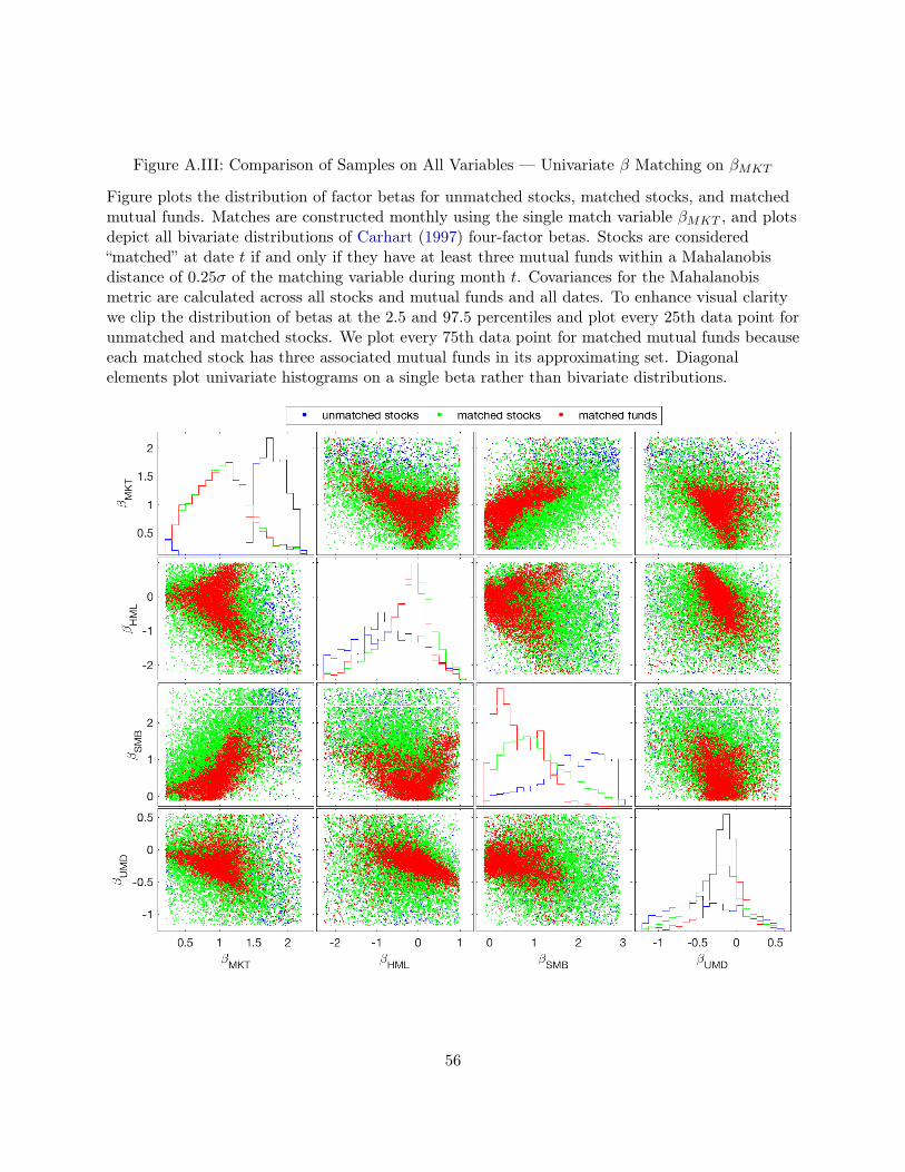
Figure A.III: Comparison of Samples on All Variables — Univariate � Matching on �MKT
Figure plots the distribution of factor betas for unmatched stocks, matched stocks, and matchedmutual funds. Matches are constructed monthly using the single match variable �MKT , and plotsdepict all bivariate distributions of Carhart (1997) four-factor betas. Stocks are considered“matched” at date t if and only if they have at least three mutual funds within a Mahalanobisdistance of 0.25� of the matching variable during month t. Covariances for the Mahalanobismetric are calculated across all stocks and mutual funds and all dates. To enhance visual claritywe clip the distribution of betas at the 2.5 and 97.5 percentiles and plot every 25th data point forunmatched and matched stocks. We plot every 75th data point for matched mutual funds becauseeach matched stock has three associated mutual funds in its approximating set. Diagonalelements plot univariate histograms on a single beta rather than bivariate distributions.
56

Tabl
eA
.III
:Com
pari
son
ofSa
mpl
eson
Mat
chin
gVar
iabl
e—
Uni
vari
ate�
Mat
chin
gon
�M
KT
Tabl
epr
esen
tsth
edi
stri
buti
onof
fact
orbe
tasf
orun
mat
ched
stoc
ks(S
U),
mat
ched
stoc
ks(S
M),
and
mat
ched
mut
ualf
unds
(MFM
)fo
rea
chqu
inti
le(fi
rst
colu
mn)
ofth
ero
lling
mar
ket
beta
dist
ribu
tion
.M
atch
esar
eco
nstr
ucte
dm
onth
lyon
lagg
edm
arke
tbe
ta.
Stoc
ksar
eco
nsid
ered
“mat
ched
”at
date
tif
and
only
ifth
eyha
veat
leas
tth
ree
mut
ualf
unds
wit
hin
aM
ahal
anob
isdi
stan
ceof
0.25
�of
the
mat
chin
gva
riab
ledu
ring
mon
tht.
Cov
aria
nces
for
the
Mah
alan
obis
met
ric
are
calc
ulat
edac
ross
alls
tock
san
dm
utua
lfu
nds
and
alld
ates
.µ
isth
eav
erag
eva
lue
ofbe
tas
wit
hin
abi
nfo
rea
chfa
ctor
,�is
the
stan
dard
devi
atio
nof
thes
ebe
tas,
and
Nis
the
coun
tof
bin
elem
ents
.T
hefin
alro
wta
bula
tes
the
frac
tion
ofst
ocks
succ
essf
ully
mat
ched
tom
utua
lfun
ds.
All
sum
mar
yst
atis
tics
are
cons
truc
ted
acro
ssal
ldat
es.
MKT
HM
LSM
BUM
Dµ
�N
µ�
Nµ
�N
µ�
N
Sort
vari
able
Rol
ling�M
KT
Rol
ling�M
KT
Rol
ling�M
KT
Rol
ling�M
KT
Q1
SU
0.07
0.99
1944
00.
081.
5019
440
0.96
1.38
1944
0-0
.22
1.04
1944
0SM
0.62
0.35
4266
65-0
.08
0.67
4266
650.
750.
7842
6665
-0.1
60.
4342
6665
MFM
0.62
0.34
3605
78-0
.17
0.40
3605
780.
280.
3536
0578
-0.0
90.
1836
0578
Q2
SU
1.42
1.11
5488
-0.9
31.
8354
881.
991.
4854
88-0
.46
1.23
5488
SM
0.85
0.32
4475
14-0
.15
0.65
4475
140.
890.
7244
7514
-0.2
30.
3944
7514
MFM
0.85
0.32
4889
84-0
.29
0.50
4889
840.
430.
4148
8984
-0.1
30.
2048
8984
Q3
SU
1.71
0.67
1056
2-0
.97
1.32
1056
22.
160.
9710
562
-0.5
30.
9410
562
SM
1.04
0.31
4429
17-0
.28
0.71
4429
171.
070.
7444
2917
-0.2
80.
4344
2917
MFM
1.04
0.31
5336
10-0
.45
0.61
5336
100.
620.
4653
3610
-0.1
50.
2453
3610
Q4
SU
1.80
0.49
3010
1-1
.00
1.21
3010
12.
210.
8930
101
-0.5
10.
8430
101
SM
1.21
0.34
4213
83-0
.47
0.83
4213
831.
280.
8142
1383
-0.3
10.
4942
1383
MFM
1.21
0.34
4381
32-0
.64
0.71
4381
320.
820.
4743
8132
-0.1
70.
2943
8132
Q5
SU
2.14
0.65
1082
81-1
.36
1.61
1082
812.
381.
1310
8281
-0.5
51.
0610
8281
SM
1.48
0.45
3398
63-0
.75
1.18
3398
631.
611.
0033
9863
-0.3
80.
6533
9863
MFM
1.48
0.45
2550
89-0
.89
0.88
2550
891.
040.
5025
5089
-0.2
50.
3825
5089
%M
atched
92.3
%90
.4%
79.3
%83
.9%
57

Figure A.IV: Comparison of Samples on All Variables — Multivariate � Matching
Figure plots the distribution of factor betas for unmatched stocks, matched stocks, and matchedmutual funds. Matches are constructed monthly using all Carhart (1997) four-factor betas, andplots depict all bivariate distributions of these betas. Stocks are considered “matched” at date t ifand only if they have at least three mutual funds within a Mahalanobis distance of 1� of thematching variables during month t. Covariances for the Mahalanobis metric are calculated acrossall stocks and mutual funds and all dates. To enhance visual clarity we clip the distribution ofbetas at the 2.5 and 97.5 percentiles and plot every 25th data point for unmatched and matchedstocks. We plot every 75th data point for matched mutual funds because each matched stock hasthree associated mutual funds in its approximating set. Diagonal elements plot univariatehistograms on a single beta rather than bivariate distributions.
58

Tabl
eA
.IV:C
ompa
riso
nof
Sam
ples
onA
llVar
iabl
es—
Mul
tiva
riat
e�
Mat
chin
g
Tabl
epr
esen
tsth
edi
stri
buti
onof
fact
orbe
tasf
orun
mat
ched
stoc
ks(S
U),
mat
ched
stoc
ks(S
M),
and
mat
ched
mut
ualf
unds
(MFM
)fo
rea
chqu
inti
le(fi
rst
colu
mn)
ofth
eco
rres
pond
ing
char
acte
rist
ic.
Mat
ches
are
cons
truc
ted
mon
thly
onla
gged
beta
sfo
ral
lfou
rC
arha
rt(1
997)
fact
ors.
Stoc
ksar
eco
nsid
ered
“mat
ched
”at
date
tif
and
only
ifth
eyha
veat
leas
tth
ree
mut
ualf
unds
wit
hin
aM
ahal
anob
isdi
stan
ceof
1�of
mat
chin
gva
riab
les
duri
ngm
onth
t.C
ovar
ianc
esfo
rth
eM
ahal
anob
ism
etri
car
eca
lcul
ated
acro
ssal
lsto
cks
and
mut
ualf
unds
and
alld
ates
.µ
isth
eav
erag
eva
lue
ofbe
tas
wit
hin
abi
nfo
rea
chfa
ctor
,�is
the
stan
dard
devi
atio
nof
thes
ebe
tas,
andN
isth
eco
unt
ofbi
nel
emen
ts.
The
final
row
tabu
late
sth
efr
acti
onof
stoc
kssu
cces
sful
lym
atch
edto
mut
ual
fund
s.A
llsu
mm
ary
stat
isti
csar
eco
nstr
ucte
dac
ross
alld
ates
.
MKT
HM
LSM
BUM
Dµ
�N
µ�
Nµ
�N
µ�
N
Sort
vari
able
Rol
ling�M
KT
B/M
Rat
ioM
arke
tC
apit
aliz
atio
nP
rior
2-12
Ret
urn
Q1
SU
0.49
0.59
1683
04-0
.08
1.55
4057
580.
230.
6629
281
-0.2
50.
9249
6405
SM
0.60
0.27
2778
010.
100.
4730
1646
-0.0
20.
3415
3054
-0.0
70.
2127
1976
MFM
0.64
0.26
1716
080.
070.
4029
2111
0.04
0.27
1988
20-0
.05
0.17
2179
05Q
2SU
0.81
0.46
1516
810.
041.
2419
6712
0.71
0.73
5103
7-0
.21
0.68
1905
96SM
0.81
0.24
3013
210.
250.
4322
7879
0.24
0.35
1601
95-0
.06
0.18
2542
39M
FM
0.83
0.22
2455
540.
200.
3823
5285
0.23
0.30
2078
29-0
.05
0.14
2309
26Q
3SU
0.97
0.46
1759
110.
211.
1416
1542
1.03
0.79
9095
4-0
.19
0.65
1450
94SM
0.97
0.23
2775
680.
350.
4121
9685
0.43
0.37
1779
99-0
.06
0.18
2458
46M
FM
0.95
0.19
2551
070.
280.
3620
7244
0.37
0.33
1902
52-0
.04
0.14
2337
56Q
4SU
1.13
0.48
2244
450.
311.
1216
2780
1.22
0.86
1819
29-0
.19
0.65
1485
11SM
1.08
0.23
2270
390.
390.
3923
0691
0.60
0.36
2262
66-0
.05
0.18
2477
16M
FM
1.04
0.19
2002
550.
310.
3519
7346
0.50
0.32
1871
19-0
.04
0.14
2353
88Q
5SU
1.43
0.59
3287
830.
381.
1724
4166
1.36
1.23
1086
091
-0.2
00.
7430
4168
SM
1.19
0.28
1193
610.
390.
3926
1574
0.60
0.38
6721
40-0
.06
0.20
2871
97M
FM
1.14
0.25
1130
970.
310.
3420
0136
0.48
0.34
2755
98-0
.04
0.16
2389
87%
Matched
53.4
%51
.0%
48.4
%50
.1%
59