www.ondrugdelivery.com Copyright © 2012 Frederick Furness Publishing22

Few analytical results can be taken as absolute

values, and this is particularly true of a GSD!

WHAT IS A GSD?

The GSD or geometric standard deviation,

together with the mass median aerodynamic

diameter (MMAD), are the two metrics used to

describe the aerodynamic particle size distribu-

tion (APSD) both of airborne particles/aerosols

and those emitted by orally inhaled and nasal

drug delivery devices.

In broad terms, the MMAD can be viewed

as the “average particle size” while the GSD

represents the spread of particle sizes either side

of the “average”. So, the smaller the GSD, the

narrower the size distribution is, and vice versa.

CALCULATION METHODOLOGY

MMAD and GSD are both classically cal-

culated from a Log -Cumulative Mass % plot,

such as those shown in Figures 1 and 4.

Construction of this plot is well documented not

least in the governing guidances.1,2

The GSD is determined from the plot

according to Equation 1:

GSD =

The Y-axis may be expressed as Cumulative

Mass %, Z-Score, or Probits as in Figure 2.

Mathematically these are equivalent scales and

all three are in common use.

Issues arise around which calculation method-

ology should be used to process the data. In real-

ity few people use the plot directly in this way,

preferring to use some form of computational

software to do the job. However the same ques-

tion remains: what methodology should be used,

regression, interpolation, or some other method?

TESTING FOR LOG-NORMALITY

First it must be noted that while an MMAD

can be reported for any distribution, a GSD is

only valid for Log-Normal distributions. It is

therefore necessary to test if this is the case by

performing a linear regression and ensuring the

data is a good fit.

But what constitutes “a good fit”? The

default position of available products is an

R2 >0.95 which is probably too low given the

limited number of data points evaluated. The

pharmacopoeias do not give any guidance on this.

Then there is the matter of what data to

use for the regression. The US Pharmacopeia,

USP 601, infers that all the data should be

used, whereas ISO 27427 states that only data

between 10% and 90% Cumulative Mass should

be used. Some software products only use the

data between 15.87% (Probit 4) and 84.14%

(Probit 6), while others offer all of the above

as well as a dynamic approach that ensures the

core data is always properly evaluated by a true

regression (no fewer than three data points).

Let’s look at each in turn. Using all the

data can afford too much weight to the extreme

ends of the APSD distribution where recovered

masses are generally the lowest and error the

greatest.3 Using only data between 10% and 90%

Cumulative Mass removes these “extreme ends”,

but the 90% upper-limit can be counterproductive.

Consider Figure 3, the table containing

example data generated from a Next Generation

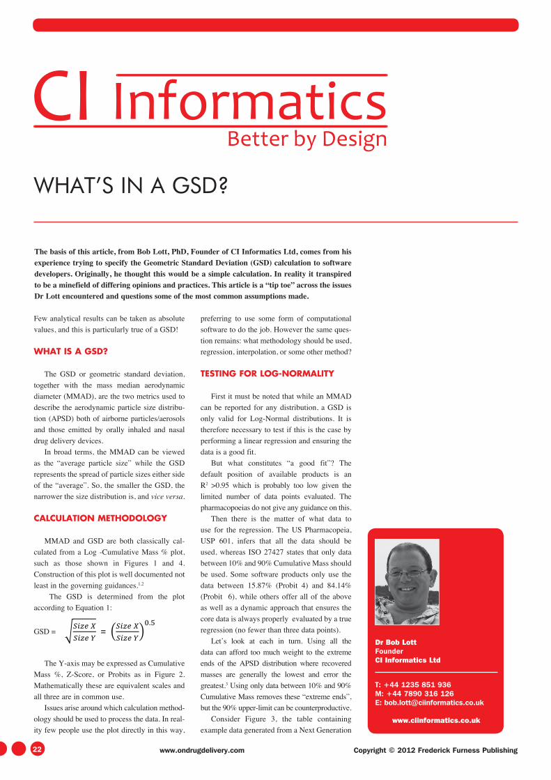
The basis of this article, from Bob Lott, PhD, Founder of CI Informatics Ltd, comes from his experience trying to specify the Geometric Standard Deviation (GSD) calculation to software developers. Originally, he thought this would be a simple calculation. In reality it transpired to be a minefield of differing opinions and practices. This article is a “tip toe” across the issues Dr Lott encountered and questions some of the most common assumptions made.

WHAT’S IN A GSD?

Dr Bob Lott FounderCI Informatics Ltd

T: +44 1235 851 936M: +44 7890 316 126E: bob.lott@ciinformatics.co.uk

www.ciinformatics.co.uk

0907_GF_ONdrugDelivery November 2012 Pulmonary and Nasal.indd 220907_GF_ONdrugDelivery November 2012 Pulmonary and Nasal.indd 22 04/12/2012 10:1304/12/2012 10:13

Copyright © 2012 Frederick Furness Publishing www.ondrugdelivery.com

ImpactorTM (NGITM; MSP Corporation,

Shoreview, MN, US).

Applying the 90 Cumulative Mass

% upper limit excludes the data point

from Stage 2. However, Stage 2 con-

tains >16% of all the recovered material

and more than that found on Stage 5,

which would be included. Therefore the

argument that this point represents an

“extreme end” is hard to justify. Indeed

perversely the more material found on

stage 2 the less likely the data will be

used. This does not make much sense

and it could be argued that arbitrary

regression limits are not always helpful.

Using only data between 15.87% and

84.13% often renders the available data to

just two points. The regression is therefore

limited to an interpolation, guaranteed to the line-

ar! In some cases only one point will exist, render-

ing the regression analysis to a mere assumption.

A dynamic approach that takes the data point

immediately below the 15.87% particle popula-

tion, up to and including to the point immediate-

ly above the 84.13% particle population affords

the benefits of excluding the extreme ends

without applying arbitrary limits and ensures a

proper regression is performed.

To sum up so far, there would appear to be

a lack of consensus as to how we should decide

if a GSD is even to be reported, let alone how

it should be determined! For the sake of this

article however let’s say we are all agreed and a

GSD is to be calculated.

REGRESSION

Since we have already performed a regres-

sion to determine whether or not a GSD should

be reported, it would seem most sensible to

use it to calculate the result. The only case

the author can think of where it would not

be sensible would be when an inappropriate

regression methodology was used during the

Log-Normal assessment.

INTERPOLATION

Good sound reasons exist why interpolation

may be used for the calculation of MMAD,

namely that it works well for Log-Normal and

non Log-Normal distributions alike and is by

far the simplest methodology to use in the lat-

ter case.3 To be clear we are talking here about

interpolating the two data points above and

below the 50% percentile (Probit 5). Applying

these same arguments to calculation of the GSD

is questionable, as 1) a GSD is not reported if

the APSD is non-Log-Normal, and 2) basing

the result on only two data points about the

MMAD may bias the result as these data points

tend to be the “steepest” portion of the

Log-Cumulative Mass % plot so giving

a steeper slope and therefore smaller

GSD result.

THEORETICAL EXTRAPOLATION

As Size X, Size Y and the MMAD

all sit on the same straight line of a

theoretically perfect Log-Normal dis-

tribution it can be shown that:

GSD = Size X/MMAD (Equation 2) or

GSD = MMAD/Size Y (Equation 3)

However these are only true where

the arguments of the equation are deter-

mined from the same linear regression data. If

the MMAD and Size X are determined from

independent interpolations there is a risk that

the extrapolation to Size Y will not be sufficient

to the data, as not all the relevant data has been

taken into consideration. This is best seen with

the aid an example Log-Cumulative Mass %

plot, Figure 4.

Here the MMAD and Size X were found by

independent interpolations on data bracketing

Z-Score = 0 and 1 respectively. These two points

are then themselves interpolated and the result-

ant line extrapolated to Z-Score = -1 to find Size

Y. This is graphically identical to Equation 2.

From the plot it can be seen that Size Y

determined in this manner is not representative

of the data in that region. This is simply because

the method excludes the data point just below

Z-Score = -1. Figure 5 contains comparative

APSD data calculated from the distribution

shown in Figure 4.

Data in brackets were not measured accord-

ing to the method used, but were back-calculat-

ed for illustration purposes.

Note the data point just below Z-Score = -1

is Stage 5 of an NGI @30L/min, resulting in a

cut-off diameter of 2.3 μm. Size Y calculated by

regression agrees well with this and is the more

accurate result.

Consider now if Size Y were interpolated

and used with the MMAD to determine Size X

(graphical equivalent of Equation 3). Size Y is

found to be 2.33 which has good agreement with

the nearest stage cut-off diameter mentioned

above. However the GSD is determined as just

1.76. This discrepancy originates from a data

set with an R2 >0.99 (based on the four points

shown in Figure 4). Applying this methodology

to less linear data sets can only result in bigger

inconsistencies. So although Equations 2 and 3

are true, they do not produce accurate results

when misused in this way.

23

Cumulative Mass % Z-Score Probit

Size Y / D(1) 15.87 -1 4

MMAD 50 0 5

Size X / D(-1) 84.13 1 6

Stage Mass (μg) Cumulative Mass (μg) Cumulative Mass % Stage Fraction %

MOC 0.00 0.00 0.00 0.00

Stage 7 0.04 0.04 0.76 0.76

Stage 6 0.13 0.16 3.40 2.65

Stage 5 0.60 0.77 15.83 12.42

Stage 4 1.58 2.35 48.43 32.61

Stage 3 1.29 3.63 75.01 26.57

Stage 2 0.80 4.43 91.53 16.52

Stage 1 0.41 4.85 100.00 8.47

Figure 2: Table showing Y-Scale equivalence values.

Figure 3: Example NGI deposition data.

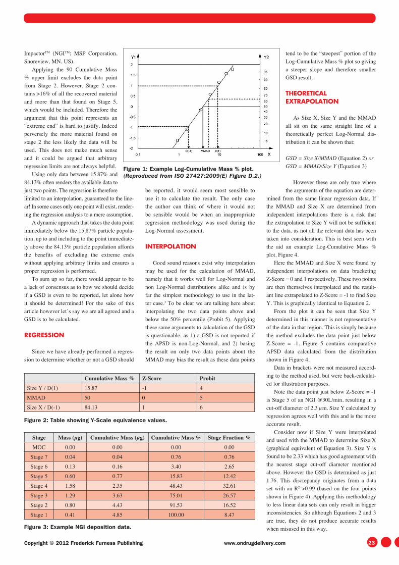
Figure 1: Example Log-Cumulative Mass % plot. (Reproduced from ISO 27427:2009(E) Figure D.2.)

0907_GF_ONdrugDelivery November 2012 Pulmonary and Nasal.indd 230907_GF_ONdrugDelivery November 2012 Pulmonary and Nasal.indd 23 04/12/2012 10:1304/12/2012 10:13

www.ondrugdelivery.com Copyright © 2012 Frederick Furness Publishing24

Using the regression data in Figure

5, Equations 2 and 3 give coherent

results. This is because both Size X

and Y are determined on an equal

basis so there is no bias for one data

point over the other.

CONCLUSIONS

If all distributions were perfectly

Log-Normal, all the methodologies dis-

cussed would give the same result, but

this is not that case and a GSD is only

ever an approximation. However some

approximations have greater mathemat-

ical integrity resulting in more accurate

results, than others.

Given the variety of practices and

regulatory requirements within the global res-

piratory drug delivery industry, it is important

for computational tools to offer the flexibility to

meet these varying demands.

REFERENCES

1. USP 34-NF 29, Physical Tests and

Determinations <601>, “Aerosols,

nasal sprays, metered-dose inhalers

and dry-powder inhalers”.

2. ISO 27427:2009(E), “Anaesthetic

and respiratory equipment nebulizing

systems and components”.

3. Stimuli to the Revision Process,

“Generalized simplified approaches

for mass median aerodynamic deter-

mination”. Pharmacopeial Forum,

2010, Vol 36(3).

ABOUT THE AUTHOR

Dr Bob Lott is founder of CI Informatics

Ltd and has worked closely with S-Matrix

Corporation (Eureka, CA, US) to bring Fusion

Inhaler Testing (FIT) to the respiratory market

place. CI Informatics is the European distribu-

tor for all S-Matrix products including Quality

by Design (QbD) solutions for respiratory prod-

uct development. Visit www.ciinformatics.co.uk

for more information.

Figure 4: Log-Z-Score plot depicting alternative methods to determine the GSD.

Methodology MMAD (μm) Size X Size Y GSD

Regression 4.35 8.58 2.21 1.97

Interpolation 4.12 7.96 2.13 1.93

Theoretical Equ. 2 4.12 8.52 (1.52) 2.07

Theoretical Equ. 3 4.12 (7.2) 2.33 1.76

Figure 5: APSD results obtained from Figure 4 using alternate calculation approaches.

0907_GF_ONdrugDelivery November 2012 Pulmonary and Nasal.indd 240907_GF_ONdrugDelivery November 2012 Pulmonary and Nasal.indd 24 04/12/2012 10:1304/12/2012 10:13