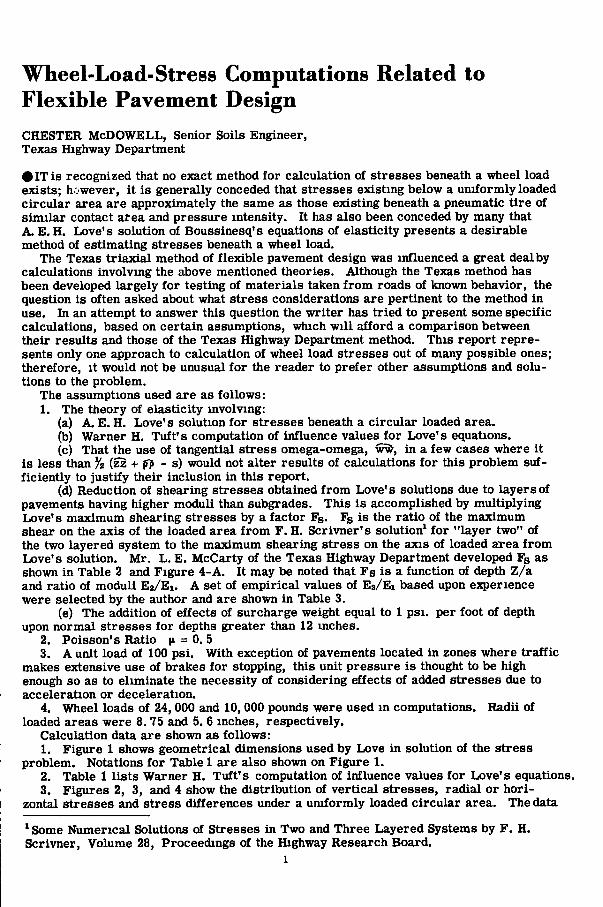
Wheel-Load-Stress Computations Related to Flexible Pavement Design CHESTER M C D O W E L L , senior Soils Engineer, Texas Highway Department

# I T i s recognized that no exact method for calculation of stresses beneath a wheel load exists; however, i t is generally conceded that stresses existing below a uniformly loaded circular area are approximately the same as those existing beneath a pneumatic tire of similar contact area and pressure intensity. It has also been conceded by many that A. E. H. Love's solution of Boussinesq's equations of elasticity presents a desirable method of estimating stresses beneath a wheel load.

The Texas triaxial method of flexible pavement design was influenced a great deal by calculations involving the above mentioned theories. Although the Texas method has been developed largely for testing of materials taken from roads of known behavior, the question is often asked about what stress considerations are pertinent to the method in use. In an attempt to answer this question the writer has tried to present some specific calculations, based on certain assumptions, which wil l afford a comparison between their results and those of the Texas Highway Department method. This report repre­sents only one approach to calculation of wheel load stresses out of many possible ones; therefore, i t would not be unusual for the reader to prefer other assumptions and solu­tions to the problem.

The assumptions used are as follows: 1. The theory of elasticity involving:

(a) A.E. H. Love's solution for stresses beneath a circular loaded area. (b) Warner H. Tuft's computation of influence values for Love's equations. (c) That the use of tangential stress omega-omega, wi^, in a few cases where i t

is less than (zz + - s) would not alter results of calculations for this problem suf­ficiently to justify their inclusion in this report.

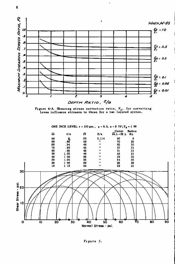
(d) Reduction of shearing stresses obtained from Love's solutions due to layers of pavements having higher moduli than subgrades. This is accomplished by multiplying Love's maximum shearing stresses by a factor Fs. Fs is the ratio of the maximum shear on the axis of the loaded area from F. H. Scrivner's solution* for "layer two" of the two layered system to the maximum shearing stress on the axis of loaded area from Love's solution. Mr. L. E. McCarty of the Texas Highway Department developed Fg as shown in Table 2 and Figure 4-A. It may be noted that Fs is a function of depth Z/a and ratio of moduli Eg/Ei. A set of empirical values of Ez/Ei based upon experience were selected by the author and are shown in Table 3.

(e) The addition of effects of surcharge weight equal to 1 psi. per foot of depth upon normal stresses for depths greater than 12 inches.

2. Poisson's Ratio = 0. 5 3. A unit load of 100 psi. With exception of pavements located in zones where traffic

makes extensive use of brakes for stopping, this unit pressure is thought to be high enough so as to eliminate the necessity of considering effects of added stresses due to acceleration or deceleration.

4. Wheel loads of 24, 000 and 10,000 pounds were used m computations. Radii of loaded areas were 8. 75 and 5. 6 inches, respectively.

Calculation data are shown as follows: 1. Figure 1 shows geometrical dimensions used by Love in solution of the stress

problem. Notations for Table 1 are also shown on Figure 1. 2. Table 1 lists Warner H. Tuft's computation of influence values for Love's equations. 3. Figures 2, 3, and 4 show the distribution of vertical stresses, radial or hori­

zontal stresses and stress differences under a uniformly loaded circular area. The data

* Some Numerical Solutions of Stresses in Two and Three Layered Systems by F. H. Scrivner, Volume 28, Proceedings of the Highway Research Board.

1

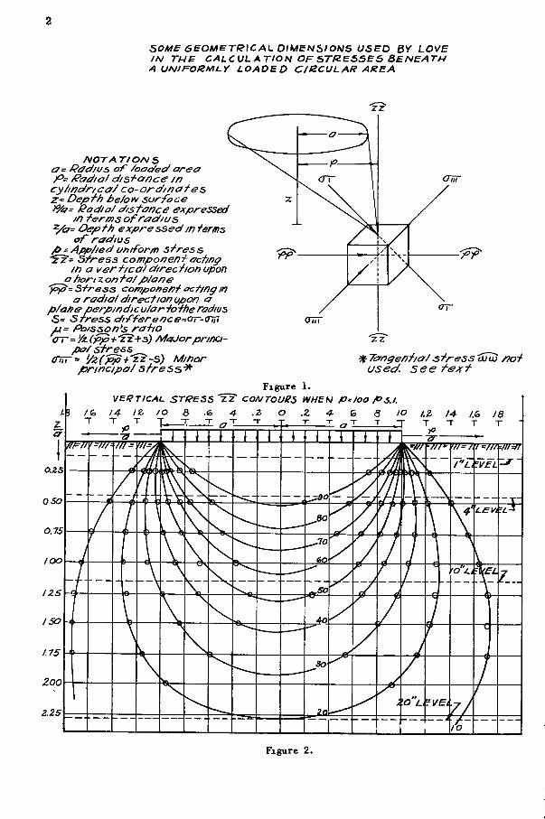
SOMe GEOMETRICAL DIMENSIONS USED BY LOVE IN THE CALC{)LATION OF STRESSES BENEATH A UNIF^O/SMLY LOADED CIRCULAR AREA

NOTATIONS a= f?ad/us of /aaa/ed area p= ^ad/a/ d/s-^once in cy/indr/ca/ co- ord/nafes z= Depth he/o^ surface >%f= ^adio/ d/staf7ce expressed

in terms of radius ^a= Depth expressed in terms

of radius p = App/ied uniform stress 'zz'= Stress component acting

in a vert/ca/d/rectionupon a hon z on ta/ p/ane

'p^= Stress component ocf/ng in a radial direcfionupon a

p/afie perpindicu/artoihe radius S= stress difference=<yr-<m ju= Po/sson*s raiio err = 'A (pp>+Tz+s) Majorprinci-

pa/ stress enrr" '/z(pp•h'z^~s) Minor

principa/ stress^

zz * Tangefrtia/ stress Unu pot

used, see te^t Figure 1.

VERTICAL STRESS zT COMTOUR5 WHEN P=IOO Ps,l. 14 IZ lO 8 •& 4 .Z O .Z 4- Q, 6 lO I.Z

m tj/v/ii'Vi=ni =miii=n

l-LEVEL

X

Figure 2.

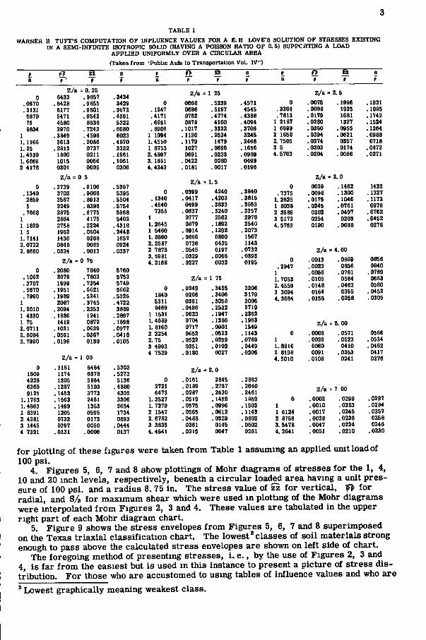
T A B L E 1

WARNER H T U F T ' S COMPUTATION O F INFLUENCE V A L U E S FOR A E . H LOVE'S SOLUTION O F STRESSES EXISTING IN A SEMI-INFINITE ISOTROPIC SOLID (HAVING A POISSON RATIO O F 0.5) SUPPCRTING A LOAD

A P P L I E D UNIFORMLY OVER A CIRCULAR AREA

(Taken Irom 'Public Aids to Transportation Vol. IV")

zz s P £p zi s P zz s a P • P p a P P p a P P P

Z / a ^ 0.25 .3424 Z/a = 1 25 Z / a = 2.5

0 6433 .9857 .3424 Z/a = 1 25 Z / a

.0670 .6428 .9855 3429 0 0668 . 5239 .4571 0 .0075 . 1996 .1921

.3131 6177 .9801 .3672 .1247 0686 .5197 4545 .3301 .0098 1935 .1885 5670 5471 .9542 .4361 .4171 0752 .4774 .4388 . 7813 .0179 1681 . 1742 75 4580 8838 5322 . 6651 0878 4100 .4094 1 2187 .0280 1327 .1524 8834 3970 .7243 .6080 . 8906 . 1017 . 3322 .3706 1 6699 .0360 .0955 .1264

1 .3849 .4596 6023 1 1094 . 1130 .2534 3245 2 1658 .0394 .0621 .0988 1. 1166 3613 .2086 .4870 1.4550 . 1179 1479 .2466 2. 7505 .0374 0357 0718 1. 25 .2812 0737 3322 1 8753 1027 .0696 . 1656 3 5 .0303 .0174 .0472 1.4330 1800 0211 . 1961 2. 4897 0691 .0233 .0909 4. 5703 .0204 .0066 .0271 1. 6869 1015 0056 . 1061 3.1651 .0422 0080 0499 2 4178 0301 0005 0306 4.4343 .0181 .0017 .0196

0 .1340 2859 5

.7668 1 1 1820 1 5 1. 7141 2. 0722 2. 8660

0 . 1062 .3707 . 5670 .7990

1 1. 2010 1 4330 1 75 2. 0711 2.6084 3. 7990

0 1609 4226 6360 9125

1.1763 1. 4663 1 8391 2 4281 3 1445 4 7321

Z / a = 0 5

. 3739 3703 3567 3249 2875 2864 2758 1962 1430 0848

.0324

.9106

.9066

.8913

.8396

.6775 4175

. 2224

.0604 0268 0085

.0013

Z / a = 0 75

.2080 2079 1999

.1951

.1989 2087

.2094

. 1886 1419

. 1031

.0561

.0196

7840 .7803 .7354 .6621 .5241 .3745 .2353

1241 0872

.0639

.0367 0130

Z / a = 1 00

. 1161 1174 1205

. 1287

. 1453

. 1563

. 1499 1205 0732 0397

.0131

6464 6378 5864 5103 3773 2461 1363 0595 0173 0050

.0006

.5367 5395

.5504

. 5754 5968 5403

.4318

.2448 1657 0924

.0337

5760 5753 5749 5662

.5326

.4722 3889

. 2897

.1698

.0977

.0418

.0105

. 5303

.5273 5136

.4880 4305 3306 2654 1734 0893

.0444 0137

Z/a = 3. 0 Z /a = 1. 5

Z /a = Z /a = 1.

0 0039 1462 1423 0 .0399 4240 .3840 .7375 .0098 1300 . 1327

. 1340 .0417 4203 .3815 1. 2625 .0175 1046 .1172

.4540 0499 3833 .3653 1 8038 .0245 0761 0976 7355 .0637 3240 . 3357 2 3989 0282 0497 .0762

1 0777 2562 2976 3 5173 0254 0203 .0452 1. 2645 0879 1892 2540 4. 5753 0190 0088 0276 1 5460 .0914 1292 .2073 1. 8660 .0866 0800 1567 2. 2587 0736 0435 1143 2 7876 .0545 0197 .0732 Z/a = 4. 00 3. 5981 4. 2168

.0329

.0227 0066 0032

.0393 0195 0

.2947 1

.0013

.0023

.0056

0869 0856 0761

0856 0840

.0789 Z/a = 1 75 1. 7053 .0105 0564 0663

0 1840 5311

.0249 0266 0361

3455 3406 3058

3206 3179 3006

2. 4559 3 3094 4. 3564

.0148 0164

.0156

0463 0355 0258

0580 .0452 .0305

8469 .0496 2532 2719 1 1531 .0623 1947 .2362 1. 4689 0704 1386 . 1963 Z/a = 5. 00 1. 8160 0717 0901 1549 Z/a = 5. 00

2 2254 0652 0523 . 1143 0 .0006 0571 0566 2.75 .0522 0259 .0769 1 .0026 0523 .0534 3 4993 0351 0102 .0449 1. 8816 0060 0410 .0462 4 7529 .0180

Z/a = 2.

0027

0

.0206 2 8198 4.5010

0091 .0108

0353 0241

0417 0276

0 .0161 2845 .2863 2721 .0189 2767 .2640 Z/a = 7 00 6473 .0287 2430 .2461 Z/a = 00

1. 3527 .0519 1459 1859 0 .0002 0299 .0297 1. 7279 .0575 0996 . 1502 1 .0010 0283 .0284 2 1547 .0565 0612 .1143 1 6124 .0017 0245 .0257 2. 6782 .0488 0329 .0802 2 8756 .0038 0236 0258 3 3835 0361 0145 .0502 3. 5478 .0047 0224 0246 4. 4641 .0215 0047 0261 4. 2641 .0051 0210 .0230

for plotting of these figures were taken from Table 1 assuming an applied umtloadof 100 psi.

4. Figures 5, 6, 7 and 8 show plottings of Mohr diagrams of stresses for the 1, 4, 10 and 20 inch levels, respectively, beneath a circular loaded area having a unit pres­sure of 100 psi. and a radius 8.75 in. The stress value of zz for vertical, for radial, and S/g for maximum shear which were used in plotting of the Mohr diagrams were interpolated from Figures 2, 3 and 4. These values are tabulated in the upper right part of each Mohr diagram chart.

5. Figure 9 shows the stress envelopes from Figures 5, 6, 7 and 8 superimposed on the Texas triaxial classification chart. The lowest ̂ classes of soil materials strong enough to pass above the calculated stress envelopes are shown on left side of chart.

The foregoing method of presenting stresses, i . e., by the use of Figures 2, 3 and 4, is far from the easiest but is used in this instance to present a picture of stress dis­tribution. For those who are accustomed to using tables of influence values and who are ' Lowest graphically meaning weakest class.

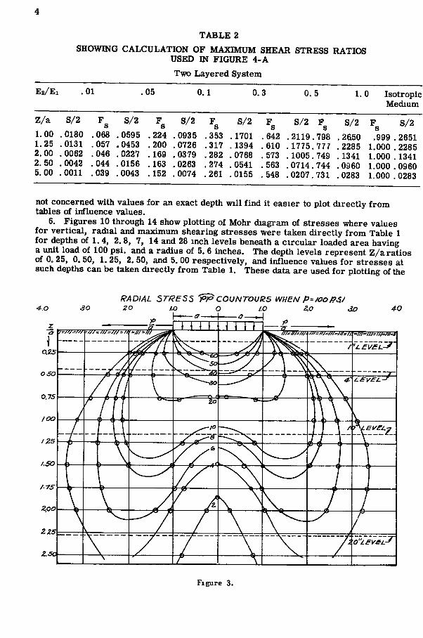
TABLE 2 SHOWING CALCULATION OF MAXIMUM SHEAR STRESS RATIOS

USED IN FIGURE 4-A Two Layered System

E2/E1 .01 ,05 0.1 0.3 0.5 1.0 Isotropic Medium

Z/a S/2 Fg S/2 F^ S/2 F^ S/2 1.00 . 0180 . 068 . 0595 . 224 . 0935 . 353 .1701 1.25 .0131 .057 .0453 .200 .0726 .317 .1394 2.00 .0062 .046 .0227 .169 .0379 .282 .0768 2.50 . 0042 . 044 . 0156 .163 . 0263 . 274 . 0541 5.00 .0011 .039 .0043 .152 .0074 .261 .0155

Fg S/2 Fg S/2 Fg S/2 .642 .2119.798 .2650 .999.2651 .610 .1775.777 .2285 1.000.2285 . 573 . 1005 . 749 . 1341 1.000 .1341 .563 .0714.744 .0960 1.000.0960 ,548 .0207.731 .0283 1.000.0283

not concerned with values for an exact depth wi l l find i t easier to plot directly from tables of influence values.

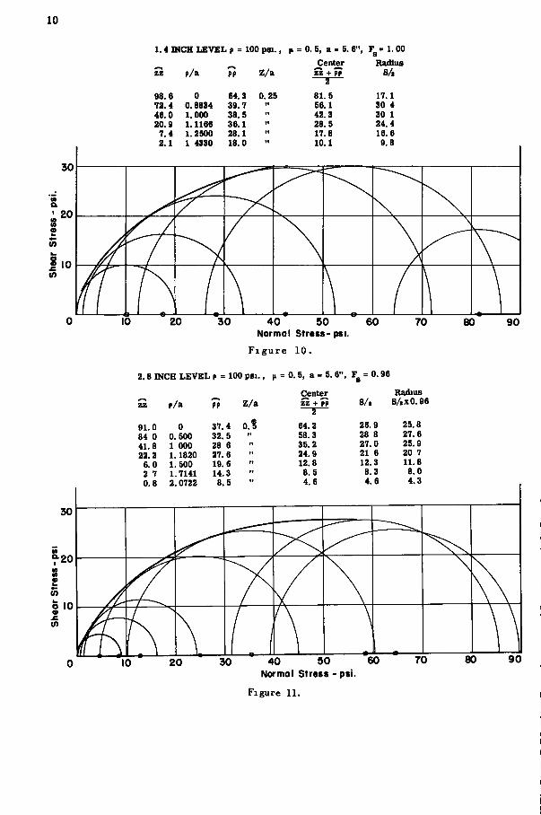
6. Figures 10 through 14 show plotting of Mohr diagram of stresses where values for vertical, radial and maximum shearing stresses were taken directly from Table 1 for depths of 1. 4, 2.8, 7, 14 and 28 inch levels beneath a circular loaded area having a unit load of 100 psi. and a radius of 5. 6 inches. The depth levels represent Z/a ratios of 0. 25, 0. 50, 1. 25, 2. 50, and 5. 00 respectively, and influence values for stresses at such depths can be taken directly from Table 1. These data are used for plotting of the

4:0 30 RADIAL STRESS IP^ COUNTOURS WHEN P^/OOP^/ 20 1,0 o 1.0 2.0 do 40

ZO LeV£L

Z.SCA

Figure 3.

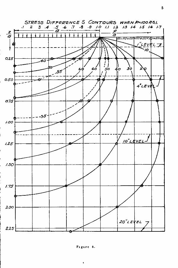
STRESS DtFFEeEA/C£ S CoNTOUR3 WHENf^^/OOf?^l. •I Z d> .4 .5 €> n Q -S /-O J.I j.Z 1-3 / . 4 1.5 /.6 /•7

a — I )0

o.zs

a so

ons

/.oo

lO

f 4 LEVS

20 LE'^EL

/.Z5

/.SO

/.7S

Z.OO

2.ZS

F i g u r e 4.

h i-o\

13

I I I A

0.3 El

^ - O.OS

= O.OI

I t 3 4 S

D£RTM RA n o , ^/a

Figure 4-A. Shearing s tress correction rat io , Fg, for converting Loves influence stresses to those for a two layered system.

30

^20

(0 10

in

10

ONE INCH L E V E L P = 100 psi. H = 0. 5, a = 8 75", Fg = 1 00 _Center Radius

zz p/a PP Z / a zz/a +p? /a S/a 96 4 85 0.114 90 8 90 .88 50 70 25 80 .94 46 " 63 30 70 .96 44 " 57 31 60 .98 42 51 31 50 1.00 40 45 31 40 1 02 38 39 30 30 1.04 38 34 30 20 1 06 36 " 28 28 10 1 12 34 " 22 21

20 30 40 50 Normal Stress - psi.

F i g u r e 5.

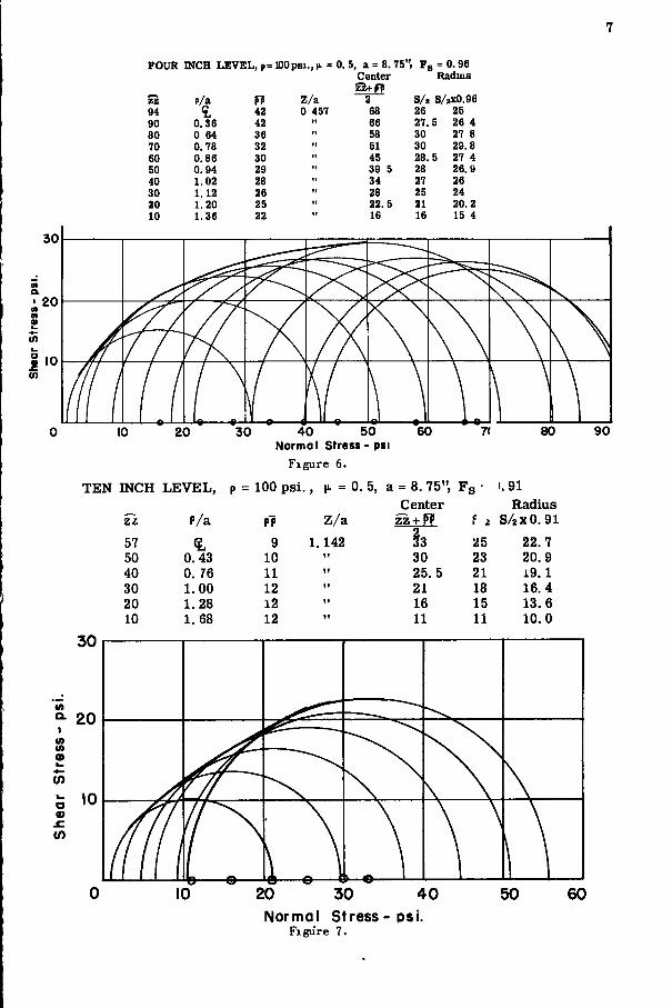
FOUR I N C H L E V E L , p= IDOpsi., IL = 0. 5, a = 8. 75", Fg = 0.96 Center Radius zz+ff

zz p/a f? Z / a 2 S/ i 8/2x0.96 94 5, 42 0 457 68 26 25 90 0.36 42 n 66 27.5 26 4 80 0 64 36 " 58 30 27 8 70 0.78 32 tt 51 30 29.8 60 0.86 30 It 45 28.5 27 4 50 0.94 29 t l 39 5 28 26.9 40 1.02 28 ,1 34 27 26 30 1.12 26 11 28 25 24 20 1.20 25 11 22.5 21 20.2 10 1.36 22 " 16 16 15 4

30

'9 » L — 1 11_Q 1 \ 1

a.

M

2 (A

| . o

10 20 30 40 50 60 7( 80 90 Normal Stress - psi

Figure 6.

INCH LEVEL, p = 100 psi. a = 8. 75", 1.91 Center Radius

Zi P/a Z/a zz + ff n

f » S/«xO. 91 57 9 1.142 §3 25 22.7 50 0. 43 10 TT 30 23 20.9 40 0. 76 11 TT 25. 5 21 19 .1 30 1.00 12 f T 21 18 16.4 20 1.28 12 TT 16 15 13.6 10 1.68 12 T! 11 11 10.0

M a. I

in o> w

3) o

30 Normal Stress - psi.

Figure 7.

60

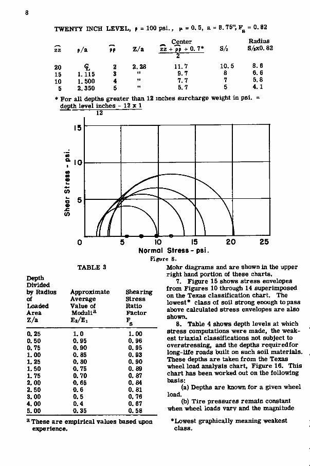
TWENTY INCH LEVEL, p = 100 psi. , K 0. 5, a = 8 .75" , F„ = 0. 82

Z Z p/a PP Z/a ^ Center Z Z + PP + 0. 7 *

2 S/2

Radius S/gxO. 82

20 15 10

5

1 . 1 1 5 1 . 5 0 0 2 . 3 5 0

2 3 4 5

2 . 2 8 »i fi tf

1 1 . 7 9 . 7 7 . 7 5 . 7

1 0 . 5 8 7 5

8 . 6 6 . 6 5 . 8 4 . 1

* For all depths greater than 12 inches surcharge weight in psi. = depth level inches - 12 x 1

12

10 Normal

Figur

TABLE 3 Depth Divided by Radius Approximate Shearing of Average Stress Loaded Value of Ratio Area Moduli* Factor Z/a E2/E1 F

s 0 . 2 5 LO LOO 0 . 5 0 0 . 9 5 0. 96 0. 75 0 . 9 0 0. 95 LOO 0 . 8 5 0. 93 L 25 0 . 8 0 0. 90 1. 50 0 . 7 5 0. 89 1. 75 0 , 7 0 0. 87 2. 00 0 . 6 5 0. 84 2. 50 0 . 6 0 . 8 1 3 . 0 0 0 . 5 0 . 7 6 4 . 0 0 0 . 4 0 . 6 7 5. 00 0 . 3 5 0 . 5 8

^ These are empirical values based upon

15 Stress - psi.

e 8. Mohr diagrams and are shown in the upper right hand portion of these charts.

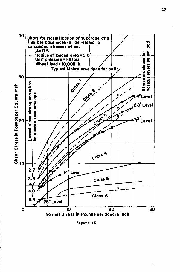
7. Figure 15 shows stress envelopes from Figures 10 through 14 superimposed on the Texas classification chart. The lowest* class of soil strong enough to pass above calculated stress envelopes are also shown.

8. Table 4 shows depth levels at which stress computations were made, the weak­est triaxial classifications not subject to overstressing, and the depths requiredfor long-life roads built on such soil materials. These depths are taken from the Texas wheel load analysis chart. Figure 16 . This chart has been worked out on the following basis:

(a) Depths are known for a given wheel load.

(b) Tire pressures remain constant when wheel loads vary and the magnitude

class.

4 0

30

1 1 1 Chart for classification of subgrade and flexible base material as related to calculated stresses when:

M=0.5 Radius of loaded area » 8.75 Unit pressure - 100 psi. Wheel load » 24,0001b.

Typical Mohr's envelopes for soils

u c

o

^ 2 0 •o c % Q.

«

h. o « JC <0

10

Level

10 20 Normal Stress in Pounds per Square Inch

F i g u r e 9.

of radii of contact areas wil l change accordingly. Then: Depth for desired design wheel load = Known depth for given wheel load

wheel load desired for design wheel load for which depths are known

A comparison of levels shown in the last and third from last column of Table 4 indi­cates that the Texas triaxial method requires approximately the same depths as those required by the theoretical concepts presented herewith.

10

1.4 INCH L E V E L p = 100 psi.

p/a PP Z / a

I* = 0. 5, a = 5. 6", Center

zz + PP

8 ^ Radius

S/,

98.6 0 64.3 0.25

2

81.5 17.1 72.4 0.8834 39. 7 56.1 30 4 46.0 1.000 38. 5 42.3 30 1 20.9 1.1166 36.1 28.5 24.4 7.4 1.2500 28.1 17.8 16.6 2.1 1 4330 18. 0 10.1 9.8

40 50 Normal Stress- psi.

F i g u r e 10.

2.8 INCH L E V E L p = 100 psi . , |i = 0. 5, a = 5. 6", F^ = 0.96

70 80 90

Center zz p/a PP Z / a zz + PP

2 SA

91.0 0 37.4 0.% 64.2 26.9 84 0 0. 500 32.5 58.3 28 8 41.8 1 000 28 6 35.2 27.0 22.2 1.1820 27.6 " 24.9 21 6

6.0 1.500 19.6 12.8 12.3 2 7 1.7141 14.3 8.5 8.3 0.8 2.0722 8.5 " 4.6 4.6

Radius S/ixO. 96

25.8 27.6 25.9 20 7 11.8 8.0 4.3

40 50 Normal Stress '

Figure 11.

11

TABLE 4 WHEEL LOAD DATA

UNIT PRESSURE = 100 PSI Depth Strength Level Class of Depth

Z/a at which Material Required Load Ratio of Calculations Required for Long-in Radius Depth to were made to Prevent Lif e Roads Lbs. (Inches) Radius (Inches) Overstress (Inches) 24,000 8. 75 0. 114 1 1 1

t t T l 0.457 4 3.0 5. 3 Tf IT 1.14 10 3.3 9.0 11 f t 2. 28 20 4.3 20. 5

10,000 5. 6 0. 25 1.4 2.7 2. 5 t f f f 0. bO 2. 8 3. 3 5. 5 TT t t 1. 25 7. 0 3. 7 9 0 Tf »T 2. 50 14. 0 4.0 11. 5 T? Tf 5.0 28. 0 6.4 28. 0

7 0 INCH L E V E L , p = 100 psi , |i = 0. 5, a = 5. 6", F = 0.90 Center Radius •

zz p/a pp Z / a zz + pp '2"

S/a S/a X 0.90

47.8 0. 4171 7. 5 1.25 27.7 22.0 19.8 41.0 0. 6651 8.8 24. 9 20. 5 18. 4 25.3 1.1094 11.3 18.3 16. 2 14. 6 14.7 1.4550 11.8 13.3 12 3 11 1 7.0 1.8753 10 3 8 6 8.3 7 5 2 3 2.4897 6.9 4.6 4. 5 4.1 0.8 3 1651 4.2 2.5 2.5 2 2

20 25 Normal Stress - psi

Figure 12.

12

14 INCH LEVEL, p = 100 psi. 0.81

zz p/a PP Z/a

20 0 0.8 2. 5 16.8 0. 7813 1.8 tf 13.3 1.2187 2.8 I I

6.2 2.1658 4.0 I I

3.6 2. 7505 3.8 I I

Center zz + PP

- , -g Radius Center zz + PP S/2 S/gx 0.81

2 10.4 9.6 7.8 9.3 8.7 7.0 8.0 7.6 6.2 5.1 5.0 4.1 3.7 3.6 2.9

I I 10 15

Normal Stress - psi.

Figure 13.

28 INCH LEVEL, p = 100 psi. , |JL = 0. 5, a = 5. 6", F„= 0. 58 Center Radius

zz p/a PP Z/a *zz + PP +1 . 3 2

S/a S/gxO. 58

5.7 0 0.1 5.0 4.2 2.8 1.6 5.2 1.000 0.3 I I 4.1 2.7 1.6 4.1 1.8816 0.6 I I 3.7 2.3 1.3 3.5 2.8196 0.9 I I 3.5 2.1 1.3 2.4 4. 5010 1.1 I I 3.1 1.8 1.0 * For all depths greater than 12 inches, surcharge weight in psi.

depth level inches - 12 x 1 12

2 3 Normal Stress - psi.

F i g u r e 14.

13

1 1 Chart for classification of subgrode and flexible base material as related to calculated stresses when:

H=0.5 Rodius of loaded area - 5.6 Unit pressure' 100psi. Wheel loads lO.OOOIb.

Typical Mohr's enve bpes for soils

Level

Level

4.0 o Class 6

Level

10 20 Normal Stress in Pounds per Square Inch

F i g u r e 15.

14

Wheel Load in Thousands of Pounds* for Long Life ( 2 0 t o 3 0 y r ) Roads

6 8 10 12

0Class Z 3 base mati

Class 2

Class 4 2 subgrade Class 3

Class 4 15

Average of ten heaviest wheel loads per overage day Depth of coverage consists of bituminous surfacing, bitu. surfoc plus base, or bitu surfacing plus plus subbose existing above mater known strength classification

Class 5

Class 6

Figure 16.

Discussion R. G. AHLVIN, Chief, Reports and Special Projects Section, Waterways Experiment Station, Vicksburg, Miss.—McDowell is to be commended for his treatment of this very difficult problem. The step from empirical to rational design methods for f lexi­ble pavements is a very large one, and McDowell has, with this paper, narrowed it somewhat.

A few minor comments appear pertinent, after which reference to an apparently re­markable correlation between the Texas Highway Department design method and the Corps of Engineers CBR design method may be of interest.

In Item 1(c) under the assumptions, the tangential stress, ww, is recognized as being the minor principal stress in a few cases. However, when Poisson's ratio is taken as 0. 5 as i t is here, the tangential stress is everywhere the intermediate principal stress. The assumption listed as Item 1(c) is therefore not needed.

It should perhaps be noted here that values of Poisson's ratio other than 0. 5 can lead to critical maximum shear stresses (or principal stress differences) up to about 20 percent larger than those computed using the 0. 5 value.

With reference to the center column of Table 3, it is not clear why the ratio of moduli, Eg/El, varies with depth. It is perhaps also notable that realistic ratios of moduli of two pavement layers, Eg/Ei, could be as low as about 0. 2 at fairly small depths.

In Figure 4, principal stress difference contours are presented. These are the same as maximum shear stress contours ( r ^ a x = "^I " '^m) except that their values are

twice as large. In our stress-distribution work at the Waterways Experiment Station we have had occasion to develop very careful and, we believe, quite accurate maximum shear stress contours. A copy of these for a Poisson's ratio of 0. 5 is shown as Figure A. The contours presented are only slightly different than those used by McDowell but they include smaller intervals between contours in the critical zone.

The relations e}q)ressed by the Texas Highway Department Flexible Pavement

1-5

28 8

OFFSET IN RAD I

Figure A.

16

WHEEL LOAD IN THOUSANDS OF POUNDS 6 a 10 12 14

CL/iSS I ao CBR

CLASS 2 so CBR

CLASS 3-A r

30 CBR

10 CBR

ASS 3-B IS CBR

10 CBR

CLASS 4-A

7 CBR

CLASS 4-B

S CBR

I CBR

Figure B.

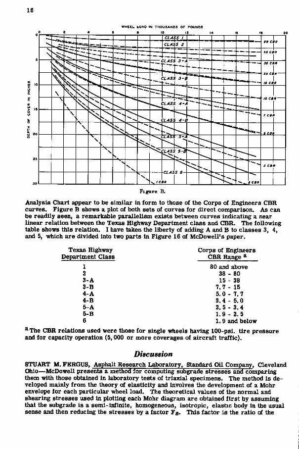
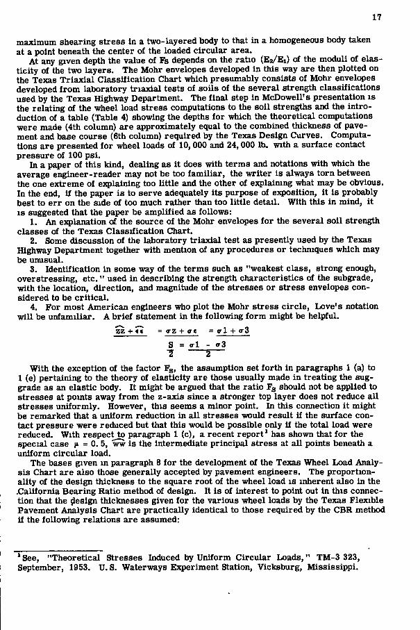
Analysis Chart appear to be similar in form to those of the Corps of Engineers CBR curves. Figure B shows a plot of both sets of curves for direct comparison. As can be readily seen, a remarkable parallelism exists between curves indicating a near linear relation between the Texas Highway Department class and CBR. The following table shows this relation. I have taken the liberty of adding A and B to classes 3, 4, and 5, which are divided into two parts in Figure 16 of McDowell's paper.

Texas Highway Department Class

Corps of Engineers CBR Range ^

1 80 and above 2 38 - 80 3-A 15 - 38 3-B 7 .7-15 4-A 5.0 - 7. 7 4-B 3. 4 - 5. 0 5-A 2. 5 - 3.4 5-B 1.9 - 2. 5 6 1.9 and below

^The CBR relations used were those for single wheels having 100-psi. tire pressure and for capacity operation (5,000 or more coverages of aircraft traffic).

Discussion STUART M. FERGUS, Asphalt Research Laboratory, Standard Oil Company, Cleveland Ohio—McDowell presents a method for computing subgrade stresses and comparing them with those obtained in laboratory tests of triaxial specimens. The method is de­veloped mainly from the theory of elasticity and involves the development of a Mohr envelope for each particular wheel load. The theoretical values of the normal and shearing stresses used in plotting each Mohr diagram are obtained f i r s t by assuming that the subgrade is a semi-infinite, homogeneous, isotropic, elastic body in the usual sense and then reducing the stresses by a factor Fg. This factor is the ratio of the

17

maximum shearing stress in a two-layered body to that in a homogeneous body taken at a point beneath the center of the loaded circular area.

At any given depth the value of Fs depends on the ratio (Eg/Ej) of the moduli of elas­ticity of the two layers. The Mohr envelopes developed in this way are then plotted on the Texas Triaxial Classification Chart which presumably consists of Mohr envelopes developed from laboratory triaxial tests of soils of the several strength classifications used by the Texas Highway Department. The final step in McDowell's presentation is the relating of the wheel load stress computations to the soil strengths and the intro­duction of a table (Table 4) showing the depths for which the theoretical computations were made (4th column) are approximately equal to the combined thickness of pave­ment and base course (6th column) required by the Texas Design Curves. Computa­tions are presented for wheel loads of 10,000 and 24,000 lb. with a surface contact pressure of 100 psi.

In a paper of this kind, dealing as i t does with terms and notations with which the average engineer-reader may not be too familiar, the writer is always torn between the one extreme of e:qplaining too little and the other of explaining what may be obvious. In the end, i f the paper is to serve adequately its purpose of exposition, i t is probably best to err on the side of too much rather than too little detail. With this in mind, i t IS suggested that the paper be amplified as follows:

1. An explanation of the source of the Mohr envelopes for the several soil strength classes of the Texas Classification Chart.

2. Some discussion of the laboratory triaxial test as presently used by the Texas Highway Department together with mention of any procedures or techniques which may be unusual.

3. Identification in some way of the terms such as "weakest class, strong enough, overstressing, etc. " used in describing the strength characteristics of the subgrade, with the location, direction, and magnitude of the stresses or stress envelopes con­sidered to be critical.

4. For most American engineers who plot the Mohr stress circle, Love's notation wil l be unfamiliar. A brief statement in the following form might be helpful.

ZZ + *e = o-z + <r« = «rl + <r3 S = <rl - <r3 T 2—

With the exception of the factor Fg, the assumption set forth in paragraphs 1 (a) to 1 (e) pertaining to the theory of elasticity are those usually made in treating the sug-grade as an elastic body. It might be argued that the ratio Fg should not be applied to stresses at points away from the z-axis since a stronger top layer does not reduce all stresses uniformly. However, this seems a minor point. In this connection i t might be remarked that a uniform reduction in all stresses would result if the surface con­tact pressure were reduced but that this would be possible only if the total load were reduced. With respect to paragraph 1 (c), a recent report* has shown that for the special case |i. = 0. 5, ww is the intermediate principal stress at all points beneath a uniform circular load.

The bases given m paragraph 8 for the development of the Texas Wheel Load Analy­sis Chart are also those generally accepted by pavement engineers. The proportion­ality of the design thickness to the square root of the wheel load is inherent also in the .California Bearing Ratio method of design. It is of interest to point out in this connec­tion that the design thicknesses given for the various wheel loads by the Texas Flexible Pavement Analysis Chart are practically identical to those required by the CBR method if the following relations are assumed:

* See, "Theoretical Stresses Induced by Uniform Circular Loads," TM-3 323, September, 1953. U. S. Waterways Experiment Station, Vicksburg, Mississippi.

18

Texas Highway Dept. Calif. Bearing Ratio Class percent

1 100 2 80 3 40 4 8 5 3.5 6 2

A wide difference of opinion, however, can be ejected on the question of the rela­tions assumed to exist between the pattern of stress distribution in a subgrade and that in a laboratory triaxial specimen. To give one example: in the ordinary trlaxial tests the lateral stress is usually held constant while the vertical stress is increased, but in a real subgrade both the lateral and the vertical stresses vary constantly between a small initial value and a maximum as the wheel load is moved on and off. It may also be pointed out that the modulus of elasticity (some writers prefer stress-strain ratio) is not a constant for soils but varies inversely with the stress. It would, therefore, seem likely that the ratio Eg/Ei is also not a constant. One result of this variability is that computations of the strain values based on summing up or on superposition of stresses are not valid. In other words, the strain produced by a stress of 50 psi. is more than 10 times that produced by a stress of 5 psi.

All of these remarks may quite correctly be considered as quibbles which do not help to produce a satisfactory theory of flexible pavement design. McDowell's paper at the very least has merit in that i t is an effort toward that goal. This reviewer, however, feels i t necessary to point out that while all the present methods of design make use in one way or another of the theory of elasticity, no method has thus far been submitted which is entirely free from empiricism.

CHESTER M C D O W E L L , closure—We are Indebted to Ahlvin for his pertinent com­ments. He states that assumption item 1(c) is not needed and for all practical purposes Ahlvin is correct. However, since i t is not obvious from Love's equations that 1(c) is not needed and since Tuft's tables of influence values indicate tensile values in one or two cases, I am not sure that the assumption can be deleted. Evidently, Ahlvin has proof of this point, and deletion of the assumption probably is in order. Ahlvin certain­ly is justified in questioning E^/Ei ratios shown by center column in Table 3 of the re­port. I can see that I failed to offer any e^qplanation of why the values were selected. There certainly are many Eg/Ei ratios other than those shown in Table 3. They may vary from 0.03 for soil-cement bases on subgrade soil to values far above one, the latter being cases where flexible bases are placed in rock cuts or over old concrete pavements. In these cases depth problems are not usually highly significant; but the selection of high quality base courses that are capable of resisting reflected stresses is important.

In cases where smaller Ez/Ei ratios exist at shallower depths than those shown, i t seems that shear stresses for similar depths and loadings should be less than those we would obtain by use of the values selected for use. For instance, shear stresses in subgrade under soil-cement or concrete are generally accepted to be lower than those in subgrade under flexible base.

It is believed that troubles arise when low Eg/Ei ratios are applied because of fa­tigue of "slab effects". In cases where "slab effects" are attained and deflections are so low that fatigue is unlikely, some reduction of overall depths are indicated due to existence of low E 2 / E 1 ratios, but we are not sure how this can be accounted for prop­erly. Therefore, i t should be stated that the E 2 / E 1 ratios shown in Table 3 are pre­ferred because shear stresses obtained by their use wil l be higher than those obtained by employment of lower ratios at similar depths. The decrease in ratio with depth is in the order of what we consider typical sections which utilize soil layers economically. See Table A for an example.

It is believed that the values in the table are on the safe side because shear stress

19

calculations obtained by their use wi l l be higher than if lower Ez/Ei ratios are em­ployed at similar depths.

TABLE A

Type of Material

Depth in Terms of Z/a

Average of Eg/El Ratio

Shearing Stress Factor Fs

Base E = 10,000 0 to 1

8500/10, 000 = 0.85 0.93 at Z/a = 1

Good Subbase E = 8, 500 1 to 2

6000/9250 = 0, 65 0.84 at Z/a = 2

Fair Subbase E = 6,000 2 to 3

3800/7625 = 0. 50 0. 76 at Z/a = 3

Select Soil E = 3,800 3 to 5

2000/5713 = 0.35 0. 58 at Z/a = 5

Subgrade E = 2000

It is interesting to note the correlation Ahlvin shows between CBR values and our strength classifications. Although I have never attempted or seen such a correlation, it is not surprising. It should be pointed out that data for the relations shown by Ahlvin were taken from similar theories of load distribution, but that actual laboratory test results do not correlate so well. For instance, many of our strength Class 3 ma­terials would have CBR values of 100 plus and this is one of the main reasons that we never did adopt the CBR method. We are just as interested in knowing what to build our bases out of as we are to know how thick they should be. So far as we are con­cerned, mold restraint is too critical in case of the CBR test when used to test base materials.

Fergus's comments certainly are of assistance in amplifying and explaining parts of the report which are not clear to the reader. He suggests that four items be ampli­fied. It should be e^qplalned that during the author's presentation of a paper (see report in HRB Research Report 16B) covering Items 1, 2 and 3 that members of the HRB Flexible Pavement Committee requested that the report be amplified by submitting comments on the type of stress analysis considered pertinent to the Texas triaxial method of flexible pavement design. It is not surprising that this report within itself appears to be rather incomplete; however, if read in conjunction with reports given in Research Report 16-B, Bulletin 93 and Volume 26 of the Proceedings of the Highway Research Board, i t wil l be much clearer to the reader.

Fergus correctly points out that the basis for development of the Texas Wheel Load Chart is the same as that used by the CBR method, but i t is not safe to assume that his tabulated correlation between CBR and strength class exists when actual tests are made. In fact some class 3 materials containing aggregate have CBR values of 100 plus. Strength class 3 materials containing small amounts to no aggregate, such as fine sand-clays, may have CBR values as low as 15. Although certain theoretical aspects of the problem correlate, i t does not necessarily follow that laboratory test results show any such correlation between CBR and Texas strength classes.

It is gratifying to note that Fergus is in agreement with Ahlvin relative to the un­importance of assumption 1(c).

Fergus points out the difficulties encountered in comparing modulus of elasticity from triaxial tests to that which develops under wheel loads. It is admitted in this in­stance that we are dealing with very elusive or variable sets of values and we do not contend that the two sets of modulae are necessarily similar. Although such E values may be dissimilar, i t does not follow that the Ez/Ei ratios derived from triaxial tests

20

are necessarily different from those produced by wheel loads because in all cases each E value used has been obtained by the same procedure.

It is admitted that the Texas Triaxial Method of Flexible Pavement Design has many empirical portions in i t without which the method would not function. The parts cover­ing testing technique of the Texas method are perhaps of more value than the theoretical parts such as are being discussed here. It is doubtful if any process or method has ever been developed from theory to practical application without some empirical steps being taken. In order to utilize methods of pavement design, i t seems desirable that they contain well balanced portions of theoretical and empirical steps. Considerable differences of opinion wil l arise as to how these portions shall be balanced.

We are indebted to Ahlvin and Fergus for their constructive and informative dis­cussions. They wil l be of assistance as developments are made in our pavement design methods.