Int J Comput Vis (2010) 86: 87–110DOI 10.1007/s11263-009-0260-y

When Discrete Meets Differential

Assessing the Stability of Structure from Small Motion

Wen-Yan Lin · Geok-Choo Tan · Loong-Fah Cheong

Received: 16 September 2008 / Accepted: 31 May 2009 / Published online: 23 June 2009© Springer Science+Business Media, LLC 2009

Abstract We provide a theoretical proof showing that un-der a proportional noise model, the discrete eight point al-gorithm behaves similarly to the differential eight point al-gorithm when the motion is small. This implies that the dis-crete algorithm can handle arbitrarily small motion for ageneral scene, as long as the noise decreases proportionallywith the amount of image motion and the proportionalityconstant is small enough. This stability result extends to allnormalized variants of the eight point algorithm. Using sim-ulations, we show that given arbitrarily small motions andproportional noise regime, the normalized eight point algo-rithms outperform their differential counterparts by a largemargin. Using real data, we show that in practical small mo-tion problems involving optical flow, these discrete structurefrom motion (SFM) algorithms also provide better estimatesthan their differential counterparts, even when the motionmagnitudes reach sub-pixel level. The better performance ofthese normalized discrete variants means that there is muchto recommend them as differential SFM algorithms that arelinear and normalized.

The support of the DSO grant R263-000-400-592 is gratefullyacknowledged.

W.-Y. Lin (�) · L.-F. CheongElectrical and Computer Engineering Department, NationalUniversity of Singapore, 4 Engineering Drive 3, Singapore117576, Singaporee-mail: linwenyan@yahoo.com

L.-F. Cheonge-mail: eleclf@nus.edu.sg

G.-C. TanDivision of Mathematical Sciences, School of Physical andMathematical Sciences, Nanyang Technological University,Singapore 637371, Singaporee-mail: gctan@ntu.edu.sg

Keywords Structure from motion · Perturbation analysis

1 Introduction

Structure from motion (SFM) is one of the oldest prob-lems in computer vision. Its goal is to obtain a 3-D motionand structure from multiple views of the same scene. Dif-ferential algorithms have been employed in SFM for manyyears. They are formulated for situations in which the mo-tion is very small, such that the said motion can be ap-proximated by velocity. To date, for nearly every discreteSFM algorithm, such as the seminal eight point algorithm byLonguet-Higgins (1981), there exists a differential counter-part (such as Longuet-Higgins and Prazdny 1980). Althoughthere are recent works reporting simulation results whichindicate that some discrete SFM algorithms appear capa-ble of handling very small motions (Baumela et al. 2000;Mainberger et al. 2008; Triggs 1999), the suspicion aboutthe stability of the discrete formulation under small motionstill persists in some quarters and has not been adequatelyaddressed theoretically. Despite the many error analysesconducted on discrete SFM (Chiuso et al. 2000; Daniilidisand Spetsakis 1997; Kanatani 2003; Luong and Faugeras1996; Ma et al. 2001; Maybank 1992; Weng et al. 1989;Xiang and Cheong 2003), there is no work that specificallylooks at the behaviour of these algorithms under increas-ingly smaller motions. All error analyses and comparisonsare invariably taken as a snapshot at a particular instanceof baseline, rather than over the entire span of baselines.What we do find are a number of anecdotal observationsstemming from the following line of analysis: at a partic-ular setting of small baseline, and given a particular set ofmotion/scene configuration, one obtains a certain set of em-pirical results and thus one accepts the hypothesis that the

88 Int J Comput Vis (2010) 86: 87–110

discrete SFM algorithm under small baseline is stable or un-stable. This lack of clear theoretical evidence continues toprompt conjectures and testing, such as: Is dense optic flowuseful to compute the fundamental matrix (Mainberger etal. 2008)? Is the first order differential computation stablerwhen the disparity is very small (Kanatani 2003)? Wouldit avoid any singular behaviour potentially present in orig-inal discrete formulation? (Ma et al. 2000 showed that asfar as linear formulation is concerned, the differential formis by no means simply a “first order approximation” of thediscrete case in the sense that a straightforward lineariza-tion of the discrete formulation results in certain terms be-ing not separable). Thus, the primary question that we seekto answer here is whether the discrete eight point formula-tion is stable even under small motion, or it faces fundamen-tal degeneracies which the differential algorithms manage toavoid by making a first order approximation.

If the answer is the former, it calls into question the mo-tivation (except for reason of efficiency) for a large vol-ume of SFM literature which by and large treat the differ-ential problem as something distinct from the discrete one.Examples of differential SFM formulations include Brookset al. (1997), Fermüller (1995), Heeger et al. (1992), Hornand Weldon (1988), Kanatani (1993), Longuet-Higgins andPrazdny (1980), Ma et al. (2000), Nister (2007) and Viévilleand Faugeras (1995). If the answer is the latter, it gives riseto the question of whether a proper understanding of the roleof differential algorithms will allow us to design better dis-crete algorithms that can handle a larger range of baselines.

1.1 The Differential Formulation

Let us begin by considering the motivation underlying dif-ferential algorithms. As the name structure from motion sug-gests, one degenerate scenario common to all SFM algo-rithms is that of a stationary camera. This degeneracy is in-trinsically insurmountable (if there is no motion, there willsurely be no structure from motion). However, it brings tomind a set of very interesting questions. How large must themotion be before we can recover structure? Is it possible torecover structure from an infinitesimally small motion? Ifso, what are the conditions required for a reasonable struc-ture recovery?

Differential SFM algorithms provide a very elegant an-swer to all of the above questions. They assert that whenthe motion is small, the movement of the individual featurepoints on the image plane can be approximated as 2D im-age velocity (which is in turn approximated by optical flow).After estimating the 2D optical flow, the differential algo-rithms seeks to compute the differential quantities definingthe cameras motion (angular velocity and translation direc-tion) and following that, the scene structure. As these al-gorithms are formulated in terms of the instantaneous mo-tion, a quantity that is independent of the amount moved,

it is clear that provided the image feature velocity (or opti-cal flow) can be extracted reasonably well, the stability ofthe algorithm is not affected by issues of whether or not amotion is “too small”.

In reality, we cannot measure the image feature velocitiesdirectly; they are actually obtained from some finite imagefeature displacements. This means that in order to carry outdifferential SFM under arbitrarily small motion, the ratio ofnoise to feature displacement magnitude (i.e. the percent-age noise) must be sufficiently small (since if the noise isof fixed magnitude, the feature displacement measurementswill eventually be overwhelmed by noise as the camera mo-tion tends to zero). In essence, the underlying premises ofthe differential formulation is that one can recover structureand motion from a sufficiently small motion, provided onehas a reasonable bound on the percentage noise in the fea-ture displacement measurements (this is equivalent to sayingthat we need a reasonable bound on the fixed noise in the ve-locity measurements).

In seeking to ascertain if the differential formulationavoids an intrinsic degeneracy present in the discrete for-mulation we need to consider whether the associated dis-crete algorithm will yield a reasonable estimate for struc-ture and motion given a sufficiently small motion and areasonable bound on the percentage noise. Henceforth, wedenote algorithms that demonstrate such behavior as be-ing able to handle “differential conditions”. We would alsolike to distinguish between the inherent sensitivity of theunderlying problem and the error properties of a particu-lar algorithm for solving that problem. For instance, try-ing to solve the SFM problem for a configuration near tothe critical surface (Maybank 1992; Negahdaripour 1989)is an inherently sensitive problem. No algorithms (discreteor differential) working with finite arithmetic precision canbe expected to obtain a solution that is not contaminatedwith large errors. In this paper, we are primarily inter-ested in the stability of the discrete SFM algorithms un-der small motion, in the sense that it does not produceany more sensitivity to perturbation than is inherent in theunderlying problem. Thus we would only deal with gen-eral scenes not close to an inherently ambiguous configu-ration.

1.2 Noise and Perturbation Analysis

We feel that a major reason for the persistent division of thetwo view problem into the differential and discrete domain isbecause it is very difficult to systematically analyze the per-formance of discrete algorithms when the motion is small.Some intuition into this problem can be obtained by lookingat the classical discrete eight point algorithm, where the es-sential matrix is obtained as the solution to the least squaresproblem min‖Ax‖2. Since the solution is in the null space

Int J Comput Vis (2010) 86: 87–110 89

of the symmetric matrix AT A, the sensitivity of the problemcan be characterized by how the eigenvalues and eigenvec-tors of the data matrix AT A is influenced by the amount ofmotion and noise. As we show later, under small motion, thedata matrix can be written as:

A(ε) ≈ AR + εAT

where the data matrix A(ε) is now written as a functionof ε. A(ε) is split into two terms: the residue term AR whenthere is no motion, and the motion term εAT , with ε → 0 asthe amount of motion becomes progressively smaller. As wewill show later, the rank of the matrix AR is at most 6, and infact, for a general scene, the rank of AR is exactly 6. SinceAR has right nullity greater than 1, as ε approaches 0 andA(ε) approaches AR , the problem of finding a unique solu-tion to the right null space of AT (ε)A(ε) becomes increas-ingly ill-conditioned as the gaps between the eigenvalues be-come smaller. In particular, if we assume that a small fixednoise N exists in the estimation process (e.g. noise arisingfrom finite arithmetic precision, which is 16 decimal digitsfor double precision):

A(ε) ≈ AR + εAT + N

then at a small enough motion, the noise N becomes com-parable or even exceeds the motion term εAT such that thelegitimate solution is no longer associated with the smallesteigenvalue of AT (ε)A(ε). This sudden appearance of a sec-ond solution has been termed as the second eigenmotion inMa et al. (2001). This ill-conditioning is the primary reasonwhy vision researchers have reservations over applying thediscrete formulation when faced with the problem of smallmotion.

However, before reaching the limit of arithmetic preci-sion, the noise is likely to be dictated by measurement noisein the feature correspondence or the optical flow (whichis actually obtained from feature displacement), and thisnoise is likely to obey a proportional model. In small mo-tion, the correspondence problem is much simplified by thefact that the two views of the scene do not differ greatlyfrom each other. There will be less hidden surfaces, smallerdifference in radiometry, and less geometrical deformation.Hence, although the motion of individual feature points issmall, the absolute error incurred in the matching processis also small. For really small motion, differential opti-cal flow algorithms (Horn and Schunck 1981; Lucas andKanade 1981) would be better placed to yield the desiredmeasurement accuracy, especially with some of the moresophisticated recent implementations (Bruhn et al. 2005;Ho and Goecke 2008; Lempitsky et al. 2008; Nir et al. 2007;Ren 2008; Sand and Teller 2006). The error in estimat-ing image velocity through the Brightness Constancy Equa-tion (BCE) has been analyzed by Verri and Poggio (1989)

from which it is clear that the noise in the flow measure-ment is also likely to be proportional to the magnitude ofthe motion. It was shown that error stems from varioussources, such as changes in the lighting arising from non-uniform illumination or different point of view, or abruptchanges in the reflectance properties of the moving surfacesat the corresponding location in space, all of which are pro-portional to the magnitude of the motion. Ohta’s analysis(Ohta 1996) approached from the perspective of the elec-tronic noise in the imaging devices and also showed thesame dependence of the measurement error in the opticalflow on the amount of image motion. This is a consequenceof the finite receptive field in real cameras, whereby thesampling function is not a Dirac’s delta function but ratherdepends on both the image gradient and the image mo-tion.

In this connection, it is also well to note that manyalgorithms for finding optical flow make errors not onlydue to the aforementioned sources, but also due to viola-tion of the flow distribution model that is assumed (suchas the smoothness assumption). This latter source of er-ror might give rise to non-proportional noise and thus pre-vent us from obtaining structure from truly infinitesimallysmall motions, even if we have succeeded in proving thestability of the discrete eight point algorithm under smallmotion with proportional noise. However, we envisage thatthese algorithm-specific errors arising from flow distribu-tion model would become smaller and smaller, especiallywith the recent spate of optical flow algorithms (Bruhn etal. 2005; Ho and Goecke 2008; Lempitsky et al. 2008;Nir et al. 2007; Ren 2008; Sand and Teller 2006) and to-gether with the publication of a database for optical flowevaluation (Baker et al. 2007). Indeed, with better flowscomputed from these algorithms in regular usage, there isgreater motivation for using flows to recover scene structuresince it avoids having to solve the tricky problem of fea-ture correspondence. It then begs the question whether weshould recover structure from flow using one of the differ-ential SFM formulations, or if inputting flows to some of thediscrete normalized variants offer a better alternative (Main-berger et al. 2008).

1.3 Findings and Organization

In this paper, we carry out perturbation analysis to studythe numerical stability of the discrete eight point algo-rithm and its variants (Chojnacki et al. 2003; Hartley, 1997;Longuet-Higgins 1981; Muhlich and Mester 1998; Torr andMurray 1997) under small motion. The noise regime thatwe have adopted is such that the data matrix A(ε) is givenby

A(ε) ≈ AR + εAT + M(ε)

90 Int J Comput Vis (2010) 86: 87–110

where M(ε) represents the inherent measurement errorsarising from various sources such as the BCE constraint andthe electronic noise, both of which are proportional to theamount of motion “ε”. We show that given a sufficientlysmall proportional noise M(ε), the discrete eight point al-gorithm and its variants are all capable of handling “dif-ferential conditions”. For researchers who view the differ-ential/discrete dichotomy as inviolate, this result is signifi-cant because much effort has been spent in refining the dis-crete eight point algorithm. It permits us to use the moreintensively researched discrete algorithms without first re-formulating the problem as a differential one; this can re-sult in very large improvements over the current state-of-the-art differential algorithms. As we show later in the ex-perimental section, the normalized discrete algorithms ap-pear to give considerably better performance than its dif-ferential counterparts (unnormalized) even when the mo-tion is extremely small. Thus one can indeed obtain a lin-ear normalized differential version by using the normal-ized 8-point discrete algorithm. For researchers who be-lieve that discrete algorithms can be readily applied tothe small motion problem, this paper provides some the-oretical explanation for their empirical results and illus-trates the limits within which such an attitude may beadopted.

The theoretical portion of the paper is primarily dividedinto three large portions. The first third of the paper (Sects. 2to 4) involves introducing the eight point formulation, withsome minor reformulations to allow rigorous analysis of itssupposed ill-conditioning in the context of small motion.The second third (Sects. 5 to 6) is primarily an adaptationof traditional perturbation theory to our problem of relatingbaseline to noise. Standard perturbation theory (Wilkinson1965) usually concerns itself with a fixed data matrix anda changing amount of noise. Our scenario is somewhat dif-ferent from the customary one: our data matrix A(ε) is alsoa function of ε. A straightforward application of standardresults would not be adequate as the Gerschgorin’s discswould overlap. Finally, in the last third of the paper (Sect. 7),we complete the stability analysis by tracking how the errorsin the fundamental matrix estimate are propagated to the ro-tation and translation estimates, from which structure of thescene is finally recovered. The theoretical analysis is thenfollowed by the experiments and the conclusion. Lastly, wealso record in the appendix some theorems and results re-quired for the perturbation analysis carried out in the paperproper.

1.4 Mathematical Notations

In this section, we explain some of the mathematical nota-tions that a reader will frequently encounter when readingthe paper.

1. AS symbolLet

A =⎡⎣

a d g

b e h

c f i

⎤⎦ .

The symbol AS denotes the vector obtained by stackingthe columns of A, i.e.,

AS = [a b c d e f g h i]T

.

2.︷︸︸︷

w symbolLet w = [w1 w2 w3 . . . w9

]T ∈ R9. We de-

note by︷︸︸︷

w the following 3 × 3 matrix

︷︸︸︷w =

⎡⎣

w1 w4 w7

w2 w5 w8

w3 w6 w9

⎤⎦ .

Clearly, we have (︷︸︸︷

w )S = w and︷︸︸︷AS = A.

3. u symbolFor each u = [u1 u2 u3

]T ∈ R3, we form the 3 × 3

skew-symmetric matrix

u =⎡⎣

0 −u3 u2

u3 0 −u1

−u2 u1 0

⎤⎦ .

(a) For v ∈ R3, we have

uv = u × v, (1)

where u × v is the vector product of u and v.(b) For a 3 × 3 invertible matrix A, with det(A) �= 0, we

have the following result from page 456 of Ma et al.(2003).

(A−1)T uA−1 = 1

det(A)(Au). (2)

4. Throughout this paper, we work on the Frobenius normof a matrix (say C) which is defined and denoted as fol-lows:

‖C‖ =√∑

i,j

c2ij .

It generalizes the definition of the usual norm on vectors.5. �x symbol

Suppose the function x(ε) is defined for ε ≥ 0. Weshall use the usual notation �x to denote the change in x:

�x = x(ε) − x(0).

Int J Comput Vis (2010) 86: 87–110 91

Likewise, we have �Yi , etc. Sometimes, to avoid cum-bersome notation, we denote a function x(ε) at ε = 0 byjust x.

6. For the ease of reading this paper, we gather in thefollowing a table of symbols for the eigenvalues andeigenvectors of the matrices AT

RAR , AT (ε)A(ε) andA(ε)T A(ε) (to be introduced in subsequent sections).

Matrix Eigenvalues Eigenvectors

ATRAR λi ri , unit vector

AT (ε)A(ε) λi(ε) qi (ε), unit vectorA(ε)T A(ε) λi(ε) qi (ε)

1.5 Mathematical Expressions

The following phrases will be frequently encountered in thispaper.

1. For a sufficiently small ε: If we say that a condition (ora statement) X is satisfied for a sufficiently small ε, itmeans that there exists a positive ε0 > 0, such that thecondition (or statement) X is satisfied for all ε where0 ≤ ε < ε0.

2. Order εn or O(εn): For an integer n, a function f (ε) issaid to be of order εn if |f (ε)| ≤ Kεn for some K > 0as ε → 0. That is, for a sufficiently small ε > 0, |f (ε)

εn | isuniformly bounded. In symbol, we write f (ε) = O(εn).When n = 0, we write O(ε0).

Some special cases/notes:(a) For a function f (ε), we note that

f (ε) = O(εn+1) ⇒ f (ε) = O(εn),

but the converse is not true in general. In other words,O(·) is not an asymptotically tight bound.

(b) If F(ε) is a matrix (or a vector), then saying it is oforder εn means that each of its individual entries is oforder εn. This is equivalent to saying that the normof F(ε) (which is a real valued function) is of orderεn.

(c) Let k be a rational number. For a sufficiently small η,we have

(1 + η)k = 1 + kη + O(η2).

This follows from the first order term of the Taylorexpansion. In particular, for non-negative real num-bers n and l, and sufficiently small ε and m, we have

(1 + O(εn)ml)k = 1 + O(εn)ml, (3)

where the constant k has been absorbed in theO-notation.

2 A Single Moving Camera Viewing a Stationary Scene

Let us assume that there is a single moving camera viewinga stationary scene consisting of N feature points Pi , where1 ≤ i ≤ N .

Let ε ≥ 0 be a non-negative real number representing theelapsed time. Our goal in this section is to formulate theeight point algorithm in the form of a data matrix and a so-lution vector, both of which can be expressed as a series in ε.Subsequently, we will use matrix perturbation theory to ana-lyze their properties when the elapsed time ε (and hence themotion) is small.

At time instance ε ≥ 0, a point Pi has its coordinates withrespect to the camera reference frame given by

Pi (ε) = [Xi(ε) Yi(ε) Zi(ε)]T

.

Let us assume that the motion is smooth, with the camerapositions being related to each other by the translation vec-tor εTc and a smoothly changing rotation R(ε). The 3 × 1vector Tc is a constant vector representing the translationalvelocity, whereas the 3 × 3 matrix R(ε) is a rotation matrixwhich changes smoothly with ε and R(0) = I , where I isthe 3 × 3 identity matrix.

The rotation matrix R(ε) can be expressed as the expo-nential of some skew-symmetric matrix ω, that is, a seriesof the form (Theorem 2.8, Ma et al. 2003)

R(ε) = I + εω + O(ε2), (4)

where ω is the angular velocity.As a result of the motion, we have

Pi (ε) = R(ε)(Pi − εTc). (5)

Recall from the preceding section that sometimes we shalldenote Pi (0) = Pi . When projected onto the image plane ofthe camera, the points Pi and Pi (ε) will have image coordi-nates pi and pi (ε) respectively where

pi = 1

Zi

Pi = [xi yi 1]T

,

(6)pi (ε) = 1

Zi(ε)Pi (ε) = [xi(ε) yi(ε) 1

]T.

Using (5) and (6), we have

pi (ε) = pi + ε[�tx �ty 0 ]T + O(ε2) (7)

where �tx, �ty are the x and y components of the imagefeature velocity respectively.

2.1 Epipolar Constraint with Normalization

Given two camera images, one at time 0 and the other attime ε, the epipolar constraint is

pTi E(ε)pi (ε) = 0, (8)

where E(ε) = TcRT (ε).

92 Int J Comput Vis (2010) 86: 87–110

Given eight or more point matches, the above epipolarconstraint is sufficient for us to determine the essential ma-trix E(ε) up to a scale factor, by solving a set of linear equa-tions.

This is the famous eight point algorithm of Longuet-Higgins (1981). However, it is important to note that theepipolar constraint is seldom used in its raw form. Rather,for the sake of numerical stability in the presence of noise, anormalization procedure is often employed.

Let Θ be an 3 × 3 invertible matrix introduced for thispurpose. For example, it can be of the form

⎡⎣

a 0 c

0 b d

0 0 1

⎤⎦ ,

with ab �= 0. Examples of normalization matrices takingsuch form are the normalization matrix in Hartley normal-ization (Hartley, 1997), or in the context of uncalibrated mo-tion analysis, Θ would be the camera’s intrinsic matrix.

For a sufficiently small ε ≥ 0, suppose

Θ(ε) = Θ + O(ε) (9)

is invertible. Then its inverse (Θ(ε))−1 takes the form

(Θ(ε))−1 = Θ−1 + O(ε). (10)

We denote the normalized (or uncalibrated) version of theessential matrix as F(ε) where

F(ε) = (ΘT )−1E(ε)(Θ(ε))−1. (11)

We will sometimes call F(ε) the fundamental matrix whereappropriate.

Using (9) and (7), we can write

Θ(ε)pi (ε) = [xi yi 1 ]T

+ ε[�tx �ty 0] + O(ε)2, (12)

where

Θpi = [xi yi 1 ]T ,

Θ(ε)pi (ε) = [xi(ε) yi(ε) 1 ]T

and (�tx,�ty) is the image feature velocity in the normal-ized system. In this normalized system, the correspondingepipolar constraint (8) becomes

[(Θpi )]T F (ε)[(Θ(ε))pi (ε)] = 0. (13)

Collecting N such constraints for i = 1, . . . ,N , we form asystem of linear equations:

A(ε)(F (ε))S = 0, (14)

where

A(ε) =⎡⎢⎣

x1(ε)x1 x1(ε)y1 x1(ε) y1(ε)x1y1(ε)y1 y1(ε) x1 y1 1...

......

......

......

......

xN(ε)xN xN(ε)yN xN(ε) yN(ε)xN yN(ε)yN yN(ε) xN yN 1

⎤⎥⎦ (15)

and (F (ε))S is the column vector defined in Sect. 1.4. Thus,an estimate of the matrix F(ε) can be obtained via the nullspace of A(ε).

Finally, we rewrite the matrix F(ε) in (11) into a formmore amenable to analysis:

F(ε) = (ΘT )−1E(ε)(Θ(ε))−1

= (Θ−1)T TcΘ−1ΘRT (ε)(Θ(ε))−1

= 1

det(Θ)[(ΘTc)][ΘRT (ε)(Θ(ε))−1] (16)

where the last step has been obtained by using (2). By (10)and (4), we have ΘRT (ε)(Θ(ε))−1 = I +O(ε) which gives

F(ε) = 1

det(Θ)[(ΘTc)][I + O(ε)]. (17)

Since F(ε) is defined up to a scale factor, we can write

F(ε) = T + O(ε) (18)

where

T = ΘTc√2‖ΘTc‖

. (19)

Here, we have set ‖T‖ = 1√2

so that (T)S has unit norm.

From (16) and (1), we note that T is in the left null space of

F(ε).

Int J Comput Vis (2010) 86: 87–110 93

3 The Degeneracy Affecting the Discrete Algorithm

Using (12), we rewrite the data matrix A(ε) as a series ex-pansion in ε,

A(ε) = AR + εAT + O(ε2) (20)

where

AR =

⎡⎢⎢⎣

x21 x1y1 x1 y1x1 y2

1 y1 x1 y1 1...

......

......

......

......

x2N xNyN xN yNxN y2

N yN xN yN 1

⎤⎥⎥⎦ ,

(21)

AT =⎡⎢⎣

x1�tx1 y1�tx1 �tx1 x1�ty1 y1�ty1 �ty1 0 0 0...

......

......

......

......

xN�txN yN�txN �txN xN�tyNyN�tyN �tyN 0 0 0

⎤⎥⎦ .

Recall that when the motion (i.e., ε) is small, the discreteeight point algorithm is regarded as increasingly ill condi-tioned. In this section, we revisit the explanation in terms ofthe data matrix A(ε).

As ε tends to zero, using (20), we know that A(ε) tendsto AR . Let F0 be a 3 × 3 matrix satisfying

(Θpi )T F0(Θ(0)pi (0)) = 0

i.e.,

(Θpi )T F0(Θpi ) = 0, (22)

which is the constraint given in (13) when ε = 0. Solving F0

from (22) is equivalent to solving the following linear leastsquares system

AR(F0)s = 0

whose solution space we will analyze now.

3.1 The Null Space of ATRAR

In this subsection, we prove that for a general scene, thenullity of the 9×9 matrix AT

RAR is 3 and we also determinethe null space of AT

RAR .Assume that the feature points on the image plane are

well distributed such that we cannot fit a conic section thatpasses through all of them (this condition is easily satisfied,especially under small motion where the number of featureswhich can be matched is very dense). We then have the fol-lowing result.

Proposition 1 Assume that all the feature points on the im-age plane do not lie on any conic section. The nullity ofAT

RAR is 3.

Proof Since

ATRARu = 0 ⇔ ARu = 0,

we shall determine the nullity of AR .

Note that the matrix AR in (21) contains 3 pairs of iden-

tical columns, namely columns 2 and 4, columns 3 and 7,

and columns 6 and 8. Hence, the rank of AR is at most 6.

Consider the submatrix A′R formed from AR by remov-

ing one copy of each repeating column pair:

A′R =

⎡⎢⎢⎣

x21 x1y1 x1 y2

1 y1 1...

......

......

...

x2N xNyN xN y2

N yN 1

⎤⎥⎥⎦ .

We shall show that the 6 columns of A′R are linearly in-

dependent so that the rank of AR is at least 6. Suppose

A′Rv = 0, where v = [a b c d e f ]T �= 0. This gives,

ax2i + bxiyi + cxi + dy2

i + eyi + f = 0, 1 ≤ i ≤ N,

which means that all the feature points lie on the conic de-

fined by ax2 + bxy + cx + dy2 + ey + f = 0. This violates

our assumption. So, we must have v = 0, which implies that

the rank of A′R (and hence AR) is at least 6. Therefore, the

rank of AR is 6. By the rank-nullity formula, the nullity of

AR is given by (9 − (rank of AR)). Hence the nullity of AR

is 3, and so is that of ATRAR . �

94 Int J Comput Vis (2010) 86: 87–110

Proposition 2 The null space of ATRAR is the following set

S = {(u)S |u ∈ R3}

=

⎧⎪⎨⎪⎩

⎡⎣

0 −u3 u2u3 0 −u1

−u2 u1 0

⎤⎦

S ∣∣∣∣∣u1, u2, u3 ∈ R

⎫⎪⎬⎪⎭

.

Proof By (1), every skew-symmetric matrix u formed fromu ∈ R

3 will satisfy (22). Thus, the set S ⊆ null space of AR .However, the set S is a subspace of R

9 and its dimensionis 3. Since the nullity of AR is also 3, the set S is indeed thenull space of AR . �

It is a well known fact that a real symmetric matrix ofthe form ZT Z has non-negative eigenvalues. Thus, we canarrange the 9 non-negative eigenvalues λi of the matrixAT

RAR in a non-increasing order:

λ1 ≥ λ2 ≥ · · · > λ7 ≥ λ8 ≥ λ9 ≥ 0.

Proposition 3 Consider the real symmetric matrix ATRAR ,

and let λi be its eigenvalue, with corresponding unit eigen-vector ri , for 1 ≤ i ≤ 9. Then we have

λ1 ≥ λ2 ≥ · · · ≥ λ6 > λ7 = λ8 = λ9 = 0.

Moreover, we may choose r7, r8 and r9 such that

r7 = T7S, r8 = T8

S, r9 = TS

where T is defined in (19), and T7, T8 and T are mutuallyorthogonal vectors of norm 1√

2.

Proof It follows from the nullity of AR (and hence ATRAR)

being 3 that the real symmetric matrix ATRAR has a zero

eigenvalue, with multiplicity 3. Thus, λ7 = λ8 = λ9 = 0.The eigen-space corresponding to the zero eigenvalue is

indeed the null space of ATRAR . Since the null space of

ATRAR is spanned by its three eigenvectors, we are free to

choose r7, r8 and r9, as long as they belong to the subspaceS in Proposition 2, and are orthonormal to each other. There-fore we choose to set

r9 = TS, (23)

where T is defined in (19).By Proposition 2, the other two eigenvectors r7 and r8

can also be written in the form r7 = T7S

, r8 = T8S

, whereT7, T8 and T must be mutually orthogonal vectors of norm

1√2

to ensure the orthonormality of r7, r8 and r9. �

Since AR has right nullity greater than 1, as ε ap-proaches 0 and A(ε) approaches AR , the problem of find-ing a unique solution to the right null space of AT (ε)A(ε)

(recall that camera pose is estimated from the right nullspace of A(ε)) becomes increasingly ill-conditioned. Thisill-conditioning is the primary reason why vision researchershave reservations over applying the discrete formulationwhen faced with the problem of small motion. However, aswe have argued in Sect. 1, if the noise in the flow estimationis proportional to ε, the question then becomes whether thenoise declining proportionally to ε is sufficient to compen-sate for the increased instability due to the last three eigen-values of AT (ε)A(ε) getting closer together. In the next sec-tion, we explain how this problem can be analyzed usingmatrix perturbation theory.

4 On the Noiseless Case A(ε)T A(ε)

The least squares solution to (14) is given by the right nullspace of the 9 × 9 symmetric matrix AT (ε)A(ε). As such,the subsequent analysis is conducted on AT (ε)A(ε) ratherthan A(ε).

If one thinks of the eigenvectors qi (ε) of AT (ε)A(ε) aspossible solutions to (14), then their corresponding eigen-values λi(ε) are the residue (sum of squared error) relatedto these solutions. That is, we have

qi (ε)T A(ε)T A(ε)qi (ε) = qi (ε)

T λi(ε)qi (ε) = λi(ε).

Thus, each λi(ε) represents the residue of A(ε) associatedwith qi (ε). The larger the value of λi(ε), for 1 ≤ i ≤ 8, themore stable is the solution as the “wrong” solution is lesslikely to be confused with the correct one.

In the absence of noise, using (20), the matrix AT (ε)A(ε)

can be expressed as the following series expansion,

AT (ε)A(ε) = ATRAR + ε(AT

T AR + ATRAT ) + O(ε2). (24)

This says that the matrix AT (ε)A(ε) can be thought ofas the “perturbation” of the matrix AT

RAR by the matrixε(AT

T AR + ATRAT ) for sufficiently small ε.

We shall use matrix perturbation theory to discuss theeigenvectors and eigenvalues of this “perturbed” matrix.

4.1 How the Eigenvectors of AT (ε)A(ε) Vary with ε

Let us denote the eigenvalues of the matrix AT (ε)A(ε) byλi(ε), i = 1,2, . . . ,9, where

λ1(ε) ≥ λ2(ε) ≥ · · · ≥ λ9(ε) ≥ 0.

We shall now choose corresponding unit eigenvectors qi (ε),for 1 ≤ i ≤ 9, such that {q1(ε),q2(ε), . . . ,q9(ε)} is an or-thonormal basis of R

9.It is clear from (16) and the definition of A(ε) in (15) that

the actual camera motion satisfies (14). Thus A(ε) and hence

Int J Comput Vis (2010) 86: 87–110 95

A(ε)T A(ε) have a nullity of at least one. In other words, wehave λ9(ε) = 0 and (F (ε))S is the corresponding eigenvec-tor.

It follows from both (18) and our choice of r9 in (23) that

(F (ε))S = r9 + O(ε).

Normalizing (F (ε))S , we obtain the unit eigenvector q9(ε) =(F (ε))S

‖(F (ε))S‖ corresponding to the eigenvalue λ9(ε) = 0. ByLemma 6 (in Appendix A.1), we have

q9(ε) = r9 + z9(ε) where z9(ε) = O(ε). (25)

Treating the matrix AT (ε)A(ε) as the “perturbation” ofthe matrix AT

RAR by ε(ATT AR + AT

RAT ) for sufficientlysmall ε, we apply perturbation theory (in particular, The-orem 8 in Appendix A.1) to obtain the following result forthe remaining unit eigenvectors of AT (ε)A(ε).

Theorem 1 The set of unit eigenvectors of AT (ε)A(ε) givenby

{q1(ε),q2(ε), . . . ,q9(ε)}can be chosen such that

qi (ε) = r′i (ε) + zi (ε),

where ‖r′i (ε)‖ = 1 and zi (ε) = O(ε). Moreover, the vectors

r′i (ε)’s have the following properties:

1. r′9(ε) = r9 = TS (from (25)).

2. r′i (ε) is a linear combination of all eigenvectors rj of

ATRAR , whose associated eigenvalue λj is identical to

λi , for i ≤ 9.3. r′

i (ε) is orthogonal to rj if λi �= λj .4. r′

i (ε), 1 ≤ i ≤ 8 is orthogonal to r9.

Remark 1 For 7 ≤ i ≤ 9, each vector r′i (ε) is a linear com-

bination of r7, r8 and r9, and hence it is a vector in the rightnull space of AR . From Proposition 2, we have

︷ ︸︸ ︷r′

7(ε) = T′7(ε), and

︷ ︸︸ ︷r′

8(ε) = T′8(ε)

for some orthogonal vectors T′7(ε) and T′

8(ε) in R3 where

‖T′7(ε)‖ = ‖T′

8(ε)‖ = ‖T‖ = 1√2.

4.2 How the Eigenvalues of AT (ε)A(ε) Vary with ε

As discussed in the preceding section, λ9(ε) = 0. For theremaining eigenvalues λi(ε), applying perturbation the-ory (Theorem 6 in Appendix A.1) to the expression forAT (ε)A(ε) in (24) yields the following result.

Proposition 4 For 1 ≤ i ≤ 8,

λi(ε) = λi + O(ε).

From Proposition 3 we know that λi > 0 for 1 ≤ i ≤ 6.As such, when ε is sufficiently small, using Proposition 4,we know that eigenvalues λi(ε) remains positive and hencetheir corresponding eigenvectors are distinct from the truesolution.

However, for 7 ≤ i ≤ 8, we note that Proposition 3 in-dicates that λi(ε) may be zero. From the point of view ofstability, this is worrying and we must seek a more explicitexpression than that offered by standard matrix perturbationtheory.

Lemma 1 For i = 7 or 8, if the hypothesis ‖A(ε)qi (ε)‖ =γiε + O(ε2) where γi > 0 is true, then λi(ε) = O(ε2). Inparticular,

λi(ε) = Λiε2 + O(ε3), where Λi = γ 2

i > 0.

Proof This follows readily from the hypothesis since

λi(ε) = qTi (ε)AT (ε)A(ε)qi (ε)

= ‖A(ε)qi (ε)‖2

= Λiε2 + O(ε3),

where Λi = γ 2i > 0. �

We shall explain why the hypothesis imposed onA(ε)qi (ε) is meaningful. Note that for 7 ≤ i ≤ 8,

A(ε)qi (ε) = (AR + εAT )(r′i (ε) + zi (ε))

= ARzi (ε) + εAT r′i (ε) + O(ε2)

= ε

(1

εARzi (ε) + AT r′

i (ε)

)+ O(ε2),

where ARzi (ε) + εAT r′i (ε) = O(ε), which is the first order

approximation of the residue of A(ε) associated with the so-lution qi (ε). The hypothesis that γi > 0 is intimately relatedto the assumption that we are dealing with a non-degeneratescene configuration in a differential setting. The reason canbe seen by looking at the square of the coefficient of the firstorder term in the preceding equation and substituting the ex-pressions for AR and AT from (21):

∥∥∥∥1

εARzi (ε) + AT r′

i (ε)

∥∥∥∥2

=N∑

j=1

((�tpj )T︷︸︸︷r′i (ε)pj + pj

T︷︸︸︷z′i (ε)pj )

2 (26)

96 Int J Comput Vis (2010) 86: 87–110

where

z′i (ε) = 1

εzi (ε) = O(ε0),

pj = [xj yj 1 ]T , �tpj = [�txj �tyj 0 ]T .

Equation (26) should be familiar to most vision re-searchers: it is the sum squared error of the differentialfundamental matrix (Ma et al. 2003; Viéville and Faugeras1995) associated with the “solution” r′

i (ε) and z′i (ε), with

r′i (ε) representing the translational velocity and z′

i (ε) relatedto the angular velocity.

From Theorem 1, for i = 7,8,︷︸︸︷r′i (ε) = T′

i (ε) where T′i (ε)

is orthogonal to the true translation T and

‖T′i (ε)‖ = 1√

2.

Thus, the positivity hypothesis made by Lemma 1 on thefirst order term γi amounts to saying that when we substi-tute with a translation vector orthogonal to the true transla-tion, the sum squared error must be greater than zero. Thishypothesis must hold, otherwise the scene in view wouldbe degenerate to the differential fundamental matrix. There-fore, using Lemma 1, we can say that

λi(ε) = ε2Λi + O(ε3), where Λi > 0,7 ≤ i ≤ 8. (27)

Hence, in principle, under noiseless condition, there is nodegeneracy in the solution to the eight point algorithm evenunder infinitesimal motion. The question of whether thisnon-degeneracy is sufficient to ensure stability under theproportional noise model is one which will investigate in thesubsequent sections.

5 Eigenvalues of AT (ε)A(ε) under Noise

Having determined how the eigenvectors and eigenvalues ofAT (ε)A(ε) vary with ε, we are now in a position to deter-mine how they are affected by noise.

Let the corrupted data matrix A(ε) be of the form

A(ε) = A(ε) + M(ε),

where A(ε) is defined in (15) and ‖M(ε)‖ ≤ εm for suffi-ciently small ε. The matrix M(ε) represents the proportionalnoise model, and m is some proportionality factor which isa function of the percentage noise in the optical flow.

Now, the matrix AT (ε)A(ε) is a perturbed version ofAT (ε)A(ε) given by

AT (ε)A(ε) = AT (ε)A(ε) + B(ε,M) (28)

where

B(ε,M) = AT (ε)M(ε) + MT (ε)A(ε) + MT (ε)M(ε)

= O(ε)m. (29)

The estimated solution is obtained by finding an eigen-vector q9(ε,M) of AT (ε)A(ε) that corresponds to its small-est eigenvalue λ9(ε,M). Thus, we have

(AT (ε)A(ε) + B(ε,M))q9(ε,M)

= λ9(ε,M)q9(ε,M). (30)

Note that both the eigenvalues λi (ε,M) and eigenvectorsqi (ε,M) of AT (ε)A(ε) are functions of ε and M . Hence-forth, we rely on the ˜ notation to remind the reader of thedependence on M , suppressing M in these cases to keep ournotation simple. However, in cases where the dependenceon M is not clear, we will explicitly write down the depen-dence.

5.1 Eigenvalue λ9(ε)

In this subsection, we shall determine the order of the eigen-value λ9(ε) via the error |λ9(ε) − λ9(ε)|, where λ9(ε) = 0.Specifically, we shall prove that λ9(ε) = O(ε2)m for a suf-ficiently small m.

Unfortunately, the standard results in perturbation theoryonly lead to |λi(ε)−λi(ε)| = O(ε)m for each i, from whichwe are not able to deduce that λ9(ε) is simple since thethree Gerschgorin’s discs might overlap. To overcome thisdifficulty, we apply the techniques developed in Wilkinson(1965) and prove a modified result of Gerschgorin’s Theo-rems, namely Proposition 8 in Appendix A.1. For readersnot familiar with Gerschgorin’s Theorems and the notion ofGerschgorin’s discs, please refer to Theorems 5 and 6 in Ap-pendix A.1.

Before we apply Proposition 8, let us record the fol-lowing simple result which plays an important role in pro-viding the order of eigenvalues and is also crucial for ob-taining the projection αi(ε,M) of q9(ε) along qi (ε) inSect. 6.

Lemma 2

(a) If either i or k is in the set {1,2,3,4,5,6}, then

‖qTk (ε)B(ε,M)qi (ε)‖ = O(ε)m.

(b) If both i and k are in the set {7,8,9}, then

‖qTk (ε)B(ε,M)qi (ε)‖ = O(ε2)m.

Int J Comput Vis (2010) 86: 87–110 97

Proof Part (a) is straightforward from (29). For part (b), weuse qi (ε) = r′

i (ε) + zi (ε) in Theorem 1, and the data matrixexpression in (20) to obtain

qTk (ε)B(ε,M)qi (ε)

= (r′k(ε) + zk(ε))

T (ATRM(ε)

+ MT (ε)AR)(r′i (ε) + zi (ε)) + O(ε2)m2.

When 7 ≤ k ≤ 9 and 7 ≤ i ≤ 9, we have λk = 0 andλi = 0. Using Theorem 1, we have ARr′

k(ε) = 0 andARr′

i (ε) = 0. Hence, we have

qTk (ε)B(ε,M)qi (ε)

= (r′k(ε) + zk(ε))

T (ATRM(ε)

+ MT (ε)AR)(r′i (ε) + zi (ε)) + O(ε2)m2

= zTk (ε)AT

RM(ε)r′i (ε) + r′T

k (ε)MT (ε)ARzi (ε)

+ zTk (ε)AT

RM(ε)zi (ε) + O(ε2)m2

= O(ε2)m. �

If we can now specially construct an invertible matrix K

such that the matrix K−1AT (ε)A(ε)K becomes a diagonalmatrix Diag(λi(ε)), then Proposition 8 provides an upperbound for |λi(ε) − λi(ε)|. Our aim is to have upper boundson |λi(ε)−λi(ε)| which enable us to isolate the 9th circulardisc G9 from the other Gi ’s.

As mentioned above, the standard result from perturba-tion theory (Wilkinson 1965) is not adequate as there re-mains a possibility that the 9th circular disc G9 defined inProposition 8 might overlap with other disc Gi , in whichcase λ9(ε) would lie in the union of the discs. We need tochoose K properly so that G9 is isolated from the other Gi .We shall now work towards a suitable choice of an invertiblematrix K .

First consider the matrix QT (ε)AT (ε)A(ε)Q(ε) whereQ(ε) is the matrix whose ith column is the unit eigenvec-tor qi (ε) of the real symmetric matrix AT (ε)A(ε). Clearly,Q−1(ε) = QT (ε). From (28), we have

QT (ε)AT (ε)A(ε)Q(ε)

= Diag(λi(ε)) + QT (ε)B(ε,M)Q(ε) (31)

where Diag(λi(ε)) is a diagonal matrix whose ith diagonalentry is λi(ε).

By Proposition 8, every eigenvalue λj (ε) of AT (ε)A(ε)

lies in at least one of the circular discs with center λk(ε) andradius

9∑i=1

|qTk (ε)B(ε,M)qi (ε)| = O(ε)m.

(Note that Proposition 8 does not imply that j is necessar-ily equal to k.) Now, the center of the 9th circular disc is 0while those of the 7th and 8th circular discs are 0 + O(ε2)

(from (27)). However, all three circular discs have radii oforder O(ε) by the preceding equation. Consequently, for asufficiently small ε, these three discs may overlap with eachother, and λ9(ε) lies in their union. As such, for this naivechoice of K = Q(ε), we are not able to ascertain a goodupper bound for |λ9(ε) − λ9(ε)|.

Fortunately, by inspecting the entries in the matrixQ(ε)T B(ε,M)Q(ε), we find that the upper bound on|λi(ε)−λi(ε)| can be improved by pre- and post-multiplyingthe matrix in (31) with the respective matrices S−1(ε) andS(ε), where

S(ε) =[εI6 00 I3

].

Here, In denotes the n × n identity matrix, and 0 is a zeromatrix. The effect of post-multiplying a matrix by S is thesame as multiplying its first six columns by ε while pre-multiplying a matrix by S−1 is the same as multiplying itsfirst six rows by 1

ε. So, we have

S−1(ε)QT (ε)B(ε,M)Q(ε)S(ε) =

⎡⎢⎢⎢⎢⎢⎢⎢⎢⎣

qT1 (ε)Bq1(ε) · · · qT

1 (ε)Bq6(ε)1εqT

1 (ε)Bq7(ε) · 1εqT

1 (ε)Bq9(ε)...

......

...

qT6 (ε)Bq1(ε) · · · qT

6 (ε)Bq6(ε)1εqT

6 (ε)Bq7(ε) · 1εqT

6 (ε)Bq9(ε)

εqT7 (ε)Bq1(ε) · · · εqT

7 (ε)Bq6(ε) qT7 (ε)Bq7(ε) · qT

7 (ε)Bq9(ε)

· · · · · · · · · · · ·εqT

9 (ε)Bq1(ε) · · · εqT9 (ε)Bq6(ε) qT

9 (ε)Bq7(ε) · qT9 (ε)Bq9(ε)

⎤⎥⎥⎥⎥⎥⎥⎥⎥⎦

98 Int J Comput Vis (2010) 86: 87–110

in which the diagonal sub-matrices of the above matrixS−1(ε)QT (ε)B(ε,M)Q(ε)S(ε) remain the same as those ofQT (ε)B(ε,M)Q(ε).

Note that the above transformation does not affect theeigenvalues. Thus, we have

S−1(ε)QT (ε)AT (ε)A(ε)Q(ε)S(ε)

= Diag(λi(ε)) + S−1(ε)QT (ε)B(ε,M)Q(ε)S(ε).

By Proposition 8, where K = Q(ε)S(ε), every eigen-value of AT (ε)A(ε) lies in at least one of the circular discsGk with center λk(ε) and radius

dk(ε,M) =

⎧⎪⎪⎪⎪⎪⎪⎪⎪⎪⎪⎪⎪⎪⎨⎪⎪⎪⎪⎪⎪⎪⎪⎪⎪⎪⎪⎪⎩

∑6i=1 |qT

k (ε)B(ε,M)qi (ε)|+ 1

ε

∑9i=7 |qT

k (ε)B(ε,M)qi (ε)|= O(ε)m, 1 ≤ k ≤ 6,

ε∑6

i=1 |qTk (ε)B(ε,M)qi (ε)|

+∑9i=7 |qT

k (ε)B(ε,M)qi (ε)|= O(ε2)m, 7 ≤ k ≤ 9.

(32)

Using the above, we may now prove that the desired prop-erty that the 9th circular disc G9 is disjoint from the rest.

Proposition 5 For a sufficiently small ε and m, the 9th cir-cular disc G9 is disjoint from the union G7 ∪ G8 of the 7thand 8th circular discs, which in turn is disjoint from theunion

⋃6i=1 Gi of the first six circular discs.

Proof First, the 9th circular disc G9 is disjoint from theunion G7 ∪ G8 of the 7th and 8th circular discs if the gap(Λ8ε

2 + O(ε3)) between the disc centers λ8(ε) and λ9(ε)

satisfies the following:

Λ8ε2 + O(ε3) > d9(ε,M)

+ max(d7(ε,M), d8(ε,M)). (33)

For a sufficiently small ε such that the left hand side is morethan 1

2Λ8ε2, and the right hand side is O(ε2)m, by (32), we

have a uniform bound on m (independent of ε) such that fora sufficiently small m, the above condition (33) is satisfied.

Next, the union⋃6

i=1 Gi of the first six circular discs is

disjoint from the union G7 ∪ G8 of the 7th and 8th circulardiscs, if the gap between the two nearest disc centers λ6(ε)

and λ7(ε) satisfies the following:

λ6(ε) − λ7(ε) > maxj=7,8

(dj (ε,M)) + max1≤k≤6

dk(ε,M).

From Proposition 4, we note that

λk(ε) = λk + O(ε) where λk > 0, for 1 ≤ k ≤ 6,

while under a non-degenerate scene, (27) holds:

λj (ε) = Λjε2 + O(ε3) where Λj > 0 for 7 ≤ j ≤ 8.

Thus the above condition is satisfied if

λ6 − Λ7ε2 + O(ε) > max

j=7,8(dj (ε,M))

+ max1≤k≤6

dk(ε,M). (34)

However, from (32), we have

maxj=7,8

(dj (ε,M)) = O(ε2)m,

and

max1≤k≤6

dk(ε,M) = O(ε)m.

Thus, since λ6 > 0, the condition (34) is satisfied for a suffi-ciently small ε when m is sufficiently small (i.e., when thereis a sufficiently small percentage noise).

Therefore, for a sufficiently small m, and a sufficientlysmall ε, the 9th circular disc G9 is disjoint from the unionG7 ∪ G8 of the 7th and 8th circular discs, which in turnis disjoint from the union

⋃6i=1 Gi of the first six circular

discs. �

It follows from the second part of Proposition 8 that λ9(ε)

lies in G9, and from (32), we record the following result:

Theorem 2 For a sufficiently small m, and a sufficientlysmall ε, the eigenvalue λ9(ε) is simple and

λ9(ε) = O(ε2)m.

Moreover,

λi (ε) = Λiε2 + O(ε2)m, i = 7,8;

(35)λi (ε) = λi + O(ε) + O(ε)m, i = 1,2,3,4,5,6.

6 Projection of q9(ε) along qk(ε)

From the preceding section, when m is small, λ9(ε) is sim-ple for sufficiently small ε. Therefore, its correspondingeigen-space is 1-dimensional. Let q9(ε) (which may not bea unit vector) be an eigenvector corresponding to the eigen-value λ9(ε) and expressed in the form

q9(ε) =9∑

i=1

αi(ε,M)qi (ε). (36)

Then the perturbation introduced to q9(ε) can be analyzedby looking at the projection coefficients αi(ε,M) using thesame technique in Wilkinson (1965).

The following result is simple yet useful in the sequel.

Int J Comput Vis (2010) 86: 87–110 99

Lemma 3

(λ9(ε) − λj (ε))αj (ε,M)

=9∑

i=1

αi(ε,M)qTj (ε)B(ε,M)qi (ε). (37)

Proof Substituting (36) into (30), and using

AT (ε)A(ε)qi (ε) = λi(ε)qi (ε),

we have

9∑i=1

αi(ε,M)λi(ε)qi (ε) +9∑

i=1

αi(ε,M)B(ε,M)qi (ε)

= λ9(ε)

(9∑

i=1

αi(ε,M)qi (ε)

).

Pre-multiplying the above equation with qTj (ε), we obtain

the required relation (37) by noting that

qTj (ε)qi (ε) =

{1, if i = j,

0, if i �= j. �

Lemma 4 Suppose the maximum projection is given by

max{|αi(ε,M)| | 1 ≤ i ≤ 9} = |αi∗(ε,M)|for some i∗ in 1 ≤ i ≤ 9. Then

|λ9(ε) − λi∗(ε)| ≤9∑

i=1

|qTj (ε)B(ε,M)qi (ε)| = O(ε)m.

Proof Dividing (37) by αi∗(ε,M) yields

(λ9(ε) − λi∗(ε)) =9∑

i=1

αi(ε,M)

αi∗(ε,M)qT

j (ε)B(ε,M)qi (ε)

with | αi(ε,M)αi∗ (ε,M)

| ≤ 1 for 1 ≤ i ≤ 9. Thus we have

|λ9(ε) − λi∗(ε)| ≤9∑

i=1

∣∣∣∣αi(ε,M)

αi∗(ε,M)qT

j (ε)B(ε,M)qi (ε)

∣∣∣∣

≤9∑

i=1

|qTj (ε)B(ε,M)qi (ε)| = O(ε)m.

The order follows from Lemma 2. �

Theorem 3 For a sufficiently small noise m (and hence M)and a sufficiently small ε, the maximum projection is givenby

max{|αi(ε,M)| |1 ≤ i ≤ 9} = |α9(ε,M)|.

Proof We first prove that for every j in 1 ≤ j ≤ 6,

|αj (ε,M)| �= max{|αi(ε,M)| |1 ≤ i ≤ 9}for a sufficiently small ε (for a given M).

Suppose on the contrary that, for some j∗ in 1 ≤j ≤ 6, there is a sequence {εs} with lims→∞ εs = 0 and|αj∗(εs,M)| = max{|αi(εs,M)| | 1 ≤ i ≤ 9}.

By Lemma 4, we have

|λ9(εs) − λj∗(εs)| ≤9∑

i=1

|qTj (εs)B(εs,M)qi (εs)|

As s → ∞, we note that the right hand side of the aboveinequality approaches 0, by Lemma 4. Using Theorem 2 andProposition 4, the left hand side approaches λj∗ , which ispositive. This yields a contradiction.

Therefore, |αj (ε,M)| is non-maximal for 1 ≤ j ≤ 6,when ε is sufficiently small.

Now, we shall prove, again by contradiction, that forevery j where 7 ≤ j ≤ 8,

|αj (ε,M)| �= max{|αi(ε,Ms)| |1 ≤ i ≤ 9}for a sufficiently small M and a sufficiently small ε.

Suppose for some j∗ ∈ {7,8}, there is a sequence{Ms} with lims→∞ ‖Ms‖ = 0 and |αj∗(ε,Ms)| =max{|αi(ε,Ms)| |1 ≤ i ≤ 9}. By Lemma 4, we have

|λ9(ε) − λj∗(ε)| ≤9∑

i=1

|qTj (ε)B(ε,Ms)qi (ε)|.

As s → ∞, we note that the right hand side approaches0, since lims→∞ ‖Ms‖ = 0. The left hand side approachesΛj∗ε

2, by Theorem 2 and Proposition 1. However, Λj∗ε2 is

positive for a sufficiently small ε > 0. This yields a contra-diction.

Therefore, for a sufficiently small m (and hence M) and asufficiently small ε, the projection |αj (ε,M)|, for 7 ≤ j ≤ 8,is non-maximal.

We conclude that for a sufficiently small m and a suffi-ciently small ε, the projection |α9(ε,M)| is maximal. �

Note that the following vector

1

α9(ε,M)q9(ε) =

9∑i=1

αi(ε,M)

α9(ε,M)qi (ε)

is an eigenvector of AT (ε)A(ε) corresponding to the eigen-value λ9(ε) with | αi(ε,M)

α9(ε,M)| ≤ 1 for 1 ≤ i ≤ 8.

Thus, from now on, for a sufficiently small ε and m, wemay assume that

q9(ε) =9∑

i=1

αi(ε,M)qi (ε), (38)

100 Int J Comput Vis (2010) 86: 87–110

where α9(ε,M) = 1 and |αi(ε,M)| ≤ 1 for 1 ≤ i ≤ 8. Notethat with α9(ε,M) = αi∗(ε,M) = 1, both Lemmas 3 and 4still apply. We shall now proceed to determine the upperbounds on αi(ε,M) for 1 ≤ i ≤ 8.

Proposition 6 For 1 ≤ j ≤ 6, for sufficiently small m and ε,we have

αj (ε,M) = O(ε)m.

Proof From Lemma 3, we have

|λ9(ε) − λj (ε)| |αj (ε,M)| ≤9∑

i=1

|qTj (ε)B(ε,M)qi (ε)|,

as each |αi(ε,M)| ≤ 1. By Theorem 2 and Proposition 1, wehave |λ9(ε) − λj (ε)| = λj + O(ε) while

9∑i=1

|qTj (ε)B(ε,M)qi (ε)| = O(ε)m,

by Lemma 2. Therefore, we have

αj (ε,M) = O(ε)m

for a sufficiently small ε and m. �

Lemma 5 For j = 7 or 8, when m is sufficiently small, wehave∣∣∣∣∣

9∑i=1

αi(ε,M)qTj (ε)B(ε,M)qi (ε)

∣∣∣∣∣= O(ε2)m.

Proof Note that

9∑i=1

|αi(ε,M)qTj (ε)B(ε,M)qi (ε)|

≤6∑

i=1

|αi(ε,M)qTj (ε)B(ε,M)qi (ε)|

+9∑

i=7

|αi(ε,M)qTj (ε)B(ε,M)qi (ε)|.

For 7 ≤ i ≤ 9, we use |αi(ε,M)| ≤ 1 and Lemma 2 to obtain

9∑i=7

|αi(ε,M)qTj (ε)B(ε,M)qi (ε)| = O(ε2)m.

For 1 ≤ i ≤ 6, by Proposition 6 and Lemma 2, we have

|αi(ε,M)qTj (ε)B(ε,M)qi (ε)| = O(ε2)m2.

Therefore,

9∑i=1

|αi(ε,M)qTj (ε)B(ε,M)qi (ε)| = O(ε2)m.

�

We have the following bound on αj (ε,M) for j = 7 or 8.

Proposition 7 For 7 ≤ j ≤ 8, for sufficiently small m andε, we have

|αj (ε,M)| = O(ε0)m.

Proof Using Lemma 3, we obtain

|αj (ε,M)| ≤∑9

i=1 |αi(ε,M)qTj (ε)B(ε,M)qi (ε)|

|λ9(ε) − λj (ε)| .

By Lemma 1 and Theorem 2, we have, for sufficiently smallε and m,

|λ9(ε) − λj (ε)| = Λjε2 + O(ε3)m

= Λjε2(1 + O(ε)m) > 0,

where Λj > 0. Therefore, together with Lemma 5, we con-clude that |αj (ε,M)| = O(ε0)m. �

As a consequence of the preceding proposition, we areable to set a uniform bound on m, i.e., independent of ε,such that |αj (ε,M)| < 1 (and are as small as we like) for7 ≤ j ≤ 8. With this m, for a sufficiently small ε > 0, wewill also have |αj (ε,M)| < 1 (and are as small as we like)for 1 ≤ j ≤ 6. The above result proves that stability of theestimated solution q9(ε) under the differential condition ofsmall motion and a bounded percentage noise.

For comparison with other statistical analysis, we wouldlike to find an explicit expression for the lowest order noiseterms (i.e., the m terms) of αj (ε,M), via (37) in conjunc-tion with the results obtained in Propositions 6 and 7 andLemma 2. We shall state and prove the result in our last the-orem:

Theorem 4 Given a sufficiently small m, and a sufficientlysmall ε,

q9(ε) =9∑

i=1

αi(ε,M)qi (ε)

where α9(ε,M) = 1,

αi(ε,M) = −qTi (ε)B(ε,M)q9(ε)

λi(ε)+ O(ε)m2

= O(ε)m, for 1 ≤ i ≤ 6,

αi(ε,M) = −qTi (ε)B(ε,M)q9(ε)

λi(ε)+ O(ε0)m2

= O(ε0)m, for 7 ≤ i ≤ 8.

Proof From (37) and (38) and Propositions 6 and 7, we have

(λ9(ε) − λj (ε))αj (ε,M)

Int J Comput Vis (2010) 86: 87–110 101

= qTj (ε)B(ε,M)q9(ε)

+8∑

i=1

αi(ε,M)qTj (ε)B(ε,M)qi (ε)

={

qTj (ε)B(ε,M)q9(ε) + O(ε)m2, 1 ≤ j ≤ 6,

qTj (ε)B(ε,M)q9(ε) + O(ε2)m2, 7 ≤ j ≤ 8.

(39)

Applying Proposition 4 and Lemma 1, we have

λ9(ε) − λj (ε) = −λj (ε)

(1 − λ9(ε)

λj (ε)

)

={

−λj (ε)(1 + O(ε2)m), if 1 ≤ j ≤ 6,

−λj (ε)(1 + O(ε0)m), if 7 ≤ j ≤ 8.

Hence, by (3), we have

1

λ9(ε) − λj (ε)={ 1

−λj (ε)(1 + O(ε2)m), if 1 ≤ j ≤ 6,

1−λj (ε)

(1 + O(ε0)m), if 7 ≤ j ≤ 8.

Dividing (39) throughout by λ9(ε) − λj (ε) and usingLemma 2, we have the desired expression stated in the the-orem. �

The above result shows that the lowest order terms innoise are the same as those derived in Wilkinson (1965),pages 70, 71, 83, where the noise is denoted by ε. It al-lows us to extend much of the unbiasedness/noise whiteninganalysis carried out on the discrete eight point algorithm tothe differential case, because the foundation of such analysisis the lowest order noise terms in the perturbation analysis.One example is the work of Muhlich and Mester (1998),which showed that for the so-called TLS-FC normalizedvariant of the discrete eight point algorithm,1 the expectedvalue of the αi(ε,M) is zero for i �= 9, that is, the estimatedsolution is unbiased.

7 Obtaining the Rotation and Translation Parameters

To complete our investigation, we need to ensure that thesubsequent decomposition of the fundamental matrix F (ε)

1In the TLS-FC variant (Muhlich and Mester 1998), matrix perturba-tion analysis was used to formulate a new data matrix A′(ε) given byA′(ε) = A(ε) + M ′(ε) = A(ε) + εM + M ′(ε), where M ′(ε) is cho-sen such that A′(ε) satisfies the rank 8 constraint without making anychanges to the columns of A(ε) in which noise is not present, andthat ‖M ′(ε)‖ is minimized. A straightforward application of the re-sult in (41) in Sect. 7 shows that this new A′(ε) is bounded by thesame proportional noise regime, and thus the results from our paperare applicable to this TLS-FC variant.

into the translation and the rotation estimates are stable. Sev-eral intermediate steps are also involved, including the cor-recting of F (ε) to the nearest rank-two matrix, and the cor-recting of the recovered essential matrix E(ε) to the nearestmatrix with the desired property of having the first two sin-gular values being equal.

In addition, to establish a proper comparison between thediscrete and the differential formulation, we need to con-vert the rotational and translational displacements recoveredfrom the discrete algorithm into the corresponding velocityformulations. As mentioned previously, the differential twoview formulation converts the SFM problem into one inde-pendent of ε but involving differential entities like velocity.Accordingly, the required orders in the errors of the discreteestimates so that the corresponding velocity estimates haveerrors independent of ε are given by:

Error in the translation direction = O(ε0)m,

Error in the rotation estimate = O(ε)m.(40)

The above means that when the discrete rotation estimateis divided by the time ε to get the rotational velocity, thelatter’s error would be independent of ε. The error in thetranslation estimate only needs O(ε0)m instead of O(ε)m

because the terms Tc and T in our formulation in fact rep-resent velocities already (see (5) and (19)). This is relatedto the fact that we can only recover the translation directionanyway.

The overall order of the error provided in Theorem 4 isO(ε0)m and superficially, does not give us much hope thatthe discrete eight point algorithm can meet the condition setout in (40) for rotation, which requires error of the orderO(ε)m. Fortunately, Theorem 4 also shows that the ordersof the perturbation coefficients αi(ε,M)′s are not all equal.In fact, only two coefficients, α7(ε,M) and α8(ε,M), are oforder O(ε0)m, whereas the rest are of order O(ε)m.

We can obtain a better bound if we split the recovered

fundamental matrix F (ε) =︷ ︸︸ ︷q9(ε) into a sum of two terms,

such that the large O(ε0)m noise only perturbs the transla-tion vector. The rest of this section and Appendix A.2 aredevoted to doing just such a split and keeping track of howthe errors are propagated and apportioned in the subsequentdecomposition into the translation and rotation estimates.

7.1 Some Preliminaries

Before proceeding further, the following short note on ‘near-est matrix’ will be used extensively in the discussion of thevarious errors throughout this section.

Let C(ε) be the noise corrupted version of a matrix C(ε).Due to the noise, C(ε) may lack some desired propertieswhich are present in C(ε) (an example of such property is

102 Int J Comput Vis (2010) 86: 87–110

that the first two singular values are identical or the rankis 2).

As is often the case, we use the ‘nearest’ C′(ε) to C(ε)

(if it exists) instead of C(ε) in the following sense:

(a) C′(ε) possesses the desired properties, and(b) ‖C′(ε) − C(ε)‖ = min{‖K − C(ε)‖ |K possesses the

desired properties}.

Thus, we have,

‖C′(ε) − C(ε)‖ ≤ ‖C(ε) − C(ε)‖. (41)

This ensures that in using the nearest matrix, the ‘correction’introduced has the same order of error.

Note that the essential/fundamental matrix is only de-fined up to a scale factor. We regard the ‘true’ fundamentalmatrix Ft (ε) as one having unit Frobenius norm and givenby

Ft(ε) =︷ ︸︸ ︷q9(ε) = TtΘRT (ε)(Θ(ε))−1 (42)

where Tt is parallel to T defined in (19) but scaled such that‖Ft(ε)‖ = 1. The true essential matrix Et(ε) is defined asthe de-normalized version of Ft(ε),

Et(ε) = ΘT Ft (ε)Θ(ε) = ΘT TtΘRT (ε). (43)

The estimated fundamental matrix is given by

F (ε) =︷ ︸︸ ︷q9(ε) .

With noise,︷ ︸︸ ︷q9(ε) may not be a unit vector and thus may

not have unit norm. Letting F (ε) stay un-normalized hasthe virtue of keeping the following proof simple while stillobtaining error expressions that suffice for our purpose.

7.2 Splitting the Fundamental Matrix

We know from Theorems 1 and 4 that our estimated solutionvector q9(ε) can be expressed as

q9(ε) = q9(ε) +8∑

i=7

αi(ε,M)r′i (ε) +

8∑i=7

αi(ε,M)zi (ε)

+6∑

i=1

αi(ε,M)qi (ε)

= q9(ε) +8∑

i=7

αi(ε,M)r′i (ε) + O(ε)m,

where

︷︸︸︷r′i (ε) = T′

i (ε), 7 ≤ i ≤ 8.

Therefore, using the definition of Ft(ε) in (42), we have

F (ε) =︷ ︸︸ ︷q9(ε)

= Ft(ε) +8∑

i=7

αi(ε,M)T′i (ε) + O(ε)m. (44)

Utilizing the relation ΘRT (ε)(Θ(ε))−1 − I = O(ε), wecan modify (44) such that

F (ε) = Ft(ε) +8∑

i=7

αi(ε,M)T′i (ε){ΘRT (ε)(Θ(ε))−1

+ O(ε)} + O(ε)m

= Fa(ε,M) + O(ε)m

where

Fa(ε,M) = Ft (ε) +(

8∑i=7

αi(ε,M)T′i (ε)

)

× ΘRT (ε)(Θ(ε))−1

= Ft (ε) + O(ε0)m (45)

is a part of F (ε) that contains the true rotation but an in-correct translation. As F (ε) may lack the rank two propertyassociated with a fundamental matrix, we apply the algo-rithm described in Ma et al. (2003) that chooses a rank 2matrix F ′(ε) with the minimum ‖F (ε)− F ′(ε)‖. If we con-sider F (ε) to be a perturbed version of the valid fundamentalmatrix Fa(ε,M) (i.e., having rank 2), then from (41),

‖F (ε) − F ′(ε)‖ ≤ ‖F (ε) − Fa(ε,M)‖ = O(ε)m.

Hence, the error in F ′(ε) takes the form

F ′(ε) = Fa(ε,M) + O(ε)m.

7.3 Errors in the Motion Estimates

The essential matrix E(ε) is obtained by de-normalizingF ′(ε):

E(ε) = ΘT F ′(ε)Θ(ε) = Ea(ε,M) + O(ε)m (46)

where using (2), (43) and (45), we have

Ea(ε,M)

= ΘT Fa(ε,M)Θ(ε)

=(

ΘT TtΘ + det(Θ)

8∑i=7

αi(ε,M) Θ−1T′i (ε)

)RT (ε)

= Et(ε) + O(ε0)m. (47)

Int J Comput Vis (2010) 86: 87–110 103

Observe that from (47), Ea(ε) is a valid essential matrix (inthe sense that it has rank 2 and two identical non-zero singu-lar values), since it is a product of a skew symmetric matrixand a rotation matrix R(ε) in SO(3).

We can treat E(ε) as a perturbed version of Ea(ε). There-fore, using the algorithm in Ma et al. (2003) to enforce onE(ε) the condition of having the first two singular valuesbeing equal, we can obtain a valid essential matrix E′(ε),where from (41) and (47), we have

‖E′(ε) − E(ε)‖ ≤ ‖Ea(ε,M) − E(ε)‖ = O(ε)m. (48)

Using triangle inequality and the orders from (46) and (48),we have

‖E′(ε) − Ea(ε,M)‖≤ ‖E′(ε) − E(ε)‖ + ‖Ea(ε,M) − E(ε)‖= O(ε)m. (49)

Similarly, using the orders from (46), (47) and (48), wehave

‖E′(ε) − Et(ε,M)‖≤ ‖E′(ε) − E(ε)‖ + ‖Et(ε,M) − E(ε)‖= O(ε0)m. (50)

The rest of the proof basically keeps track of how theerrors are propagated when one uses singular value de-composition on E′(ε) to obtain the rotation and transla-tion estimates. The steps are nontrivial but the argumentsare straightforward. Interested readers can refer to Appen-dix A.2 for the details. In particular, using the order in (50)and Proposition 9 in Appendix A.2, we obtain:

Error in the unit translational vector = O(ε0)m.

With regards to rotation, if one considers E′(ε) to be aperturbed version of Ea(ε) which contains the true rotation,then using the order in (49) and Proposition 10 in Appen-dix A.2, we obtain:

Error in the rotational matrix = O(ε)m,

completing the requirements set out in (40).

8 Simulation Results

We present simulation results for the following linear algo-rithms:

HN denotes the eight point algorithm using Hartley normal-ization (Hartley, 1997),

HNC denotes the eight point algorithm with Hartley nor-malization and estimated by Total Least Squares—FixedColumn (TLS-FC) (Muhlich and Mester 1998),

E denotes the un-normalized eight point algorithm(Longuet-Higgins 1981),

M denotes the differential essential matrix (Ma et al. 2000),and

S denotes the linear subspace differential algorithm (Heegeret al. 1992).

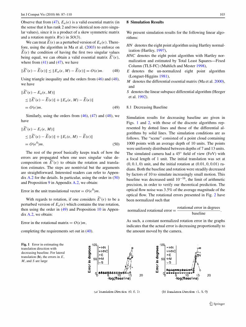
8.1 Decreasing Baseline

Simulation results for decreasing baseline are given inFigs. 1 and 2, with those of the discrete algorithms rep-resented by dotted lines and those of the differential al-gorithms by solid lines. The simulation conditions are asfollows. The “scene” consisted of a point cloud containing1000 points with an average depth of 10 units. The pointswere uniformly distributed between depths of 7 and 13 units.The simulated camera had a 45◦ field of view (FoV) witha focal length of 1 unit. The initial translation was set at(0,0.1,0) unit, and the initial rotation at (0.01,0,0.01) ra-dians. Both the baseline and rotation were steadily decreasedby factors of 10 to simulate increasingly small motion. Thisbaseline was decreased until 10−16, the limit of arithmeticprecision, in order to verify our theoretical prediction. Theoptical flow noise was 3.5% of the average magnitude of theoptical flow. The rotational errors presented in Fig. 2 havebeen normalized such that

normalized rotational error = rotational error in degrees

baseline.

As such, a constant normalized rotation error in the graphsindicates that the actual error is decreasing proportionally tothe amount moved by the camera.

Fig. 1 Error in estimating thetranslation direction withdecreasing baseline. For lateraltranslation (b), the errors in E,M , and S are large

104 Int J Comput Vis (2010) 86: 87–110

Fig. 2 Error in estimating therotation with decreasingbaseline

Fig. 3 This figure illustrates the performances of various linear algo-rithms as the noise increases. The rotation parameters for all simula-tions in this figure is given by Rotation = (0 0 0). Figures (a) to (c)

show the error in estimating the translation direction. Figures (d) to (f)show the error in estimating the rotation

8.2 Increasing Noise

The scene is similar to that in Sect. 8.1. However, in thisscenario, we fix the translation (see Fig. 3 for the transla-tion) and rotation while increasing the amount of noise. Theresults are presented in Fig. 3, with each column represent-ing different types of translational motions.

8.3 Observations

1. From Figs. 1 and 2, one can see that there was no deterio-ration in the computation of the motion parameters using

the discrete eight point algorithms (E, HN and HNC) de-

spite reductions in the baseline to the limit of arithmetic

precision. Note that the errors for the discrete algorithms

shot up at about 10−12 or 10−13: At this small baseline,

the magnitude of the optical flow, being two to three or-

ders of magnitude smaller than the baseline, reached the

limit of arithmetic precision, rendering the proportional

noise model invalid and thus resulting in the breakdown

of the discrete algorithms. This simulation clearly veri-

fies that the theoretical predictions made in the previous

section are correct.

Int J Comput Vis (2010) 86: 87–110 105

2. The performances of the differential essential matrixalgorithm (M) and the linear subspace algorithm (S)were extremely poor (Figs. 1(b) and 3), especially inthe lateral motion configuration which is susceptible tothe bas-relief ambiguity (Chiuso et al. 2000; Daniilidisand Spetsakis 1997; Ma et al. 2001; Xiang and Cheong2003). Their performances were more or less compara-ble to that of the un-normalized discrete approach (E).In contrast, the normalized discrete eight point algo-rithm with Total Least Squares—Fixed Column estima-tion (HNC) appeared to give very much superior resultseven when the motion was small, with HN ’s not far be-hind.

3. In Fig. 2, the absolute rotational error declined propor-tionally with the baseline as predicted (i.e. the rotationalerror was of the order O(ε)m).

4. Referring to Fig. 3, the impact of noise was keenly feltfor the un-normalized discrete approach (E) and the dif-ferential algorithms (M and S). Under all motion typestested, the well-known forward bias (Chiuso et al. 2000;Daniilidis and Spetsakis 1997; Ma et al. 2001) rearedits ugly head at even a low level of noise. For in-stance, in Fig. 3(c), when the noise was about 10%,the forward-biased solution of 0◦ for the translation re-sulted in an error of about 45◦ (the true translation vec-tor lies in the 45◦ direction). In the same token, forthe forward translation case (Fig. 3(a)), the excellent re-sults of E, M , and S should be treated with caution.These algorithms had a strong forward bias and irre-spective of the true motion, tended to give a forwardtranslation estimate whenever the noise was moderatelylarge. On the other hand, the normalized discrete al-gorithms (HN and HNC) exhibited much less sensitiv-ity to noise under all conditions tested, except in thetranslational estimate of HN under forward translation(Fig. 3(a)) with the noise level greater than 10%. Theresults of this simulation imply that we could expecta stable performance from the discrete HNC algorithmwhen dealing with small motions, provided that the pro-portional noise in the optical flow computation is smallenough.

9 Results on Real Image Sequences

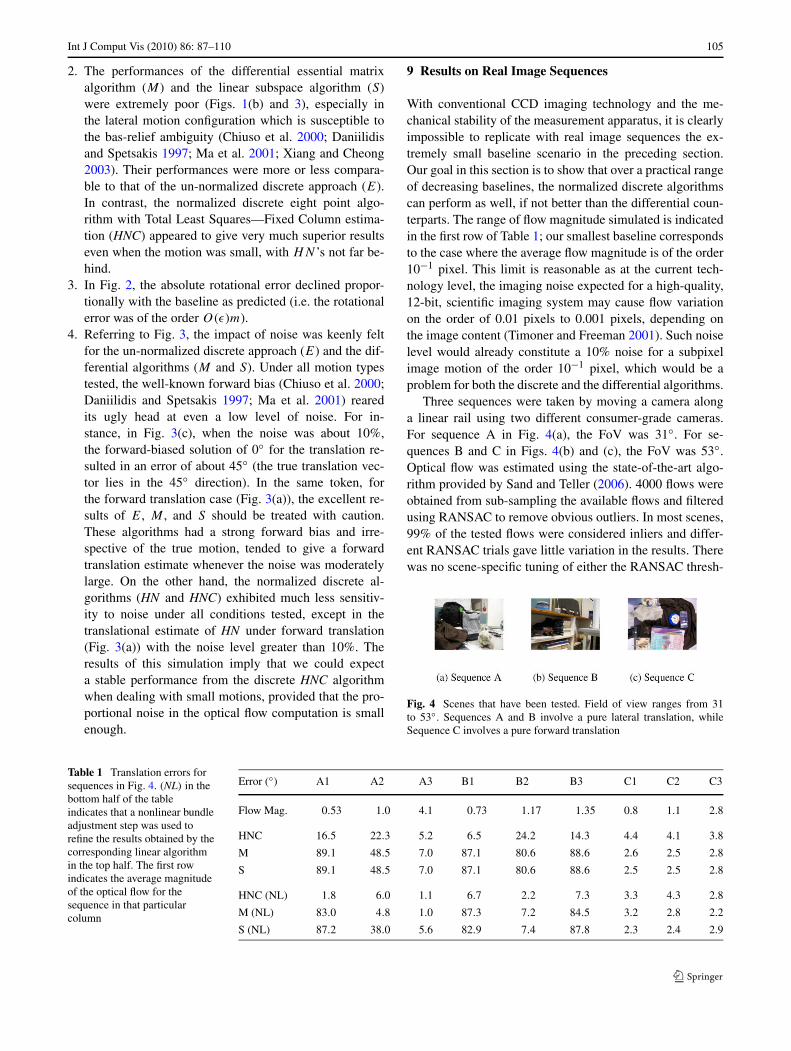
With conventional CCD imaging technology and the me-chanical stability of the measurement apparatus, it is clearlyimpossible to replicate with real image sequences the ex-tremely small baseline scenario in the preceding section.Our goal in this section is to show that over a practical rangeof decreasing baselines, the normalized discrete algorithmscan perform as well, if not better than the differential coun-terparts. The range of flow magnitude simulated is indicatedin the first row of Table 1; our smallest baseline correspondsto the case where the average flow magnitude is of the order10−1 pixel. This limit is reasonable as at the current tech-nology level, the imaging noise expected for a high-quality,12-bit, scientific imaging system may cause flow variationon the order of 0.01 pixels to 0.001 pixels, depending onthe image content (Timoner and Freeman 2001). Such noiselevel would already constitute a 10% noise for a subpixelimage motion of the order 10−1 pixel, which would be aproblem for both the discrete and the differential algorithms.

Three sequences were taken by moving a camera alonga linear rail using two different consumer-grade cameras.For sequence A in Fig. 4(a), the FoV was 31◦. For se-quences B and C in Figs. 4(b) and (c), the FoV was 53◦.Optical flow was estimated using the state-of-the-art algo-rithm provided by Sand and Teller (2006). 4000 flows wereobtained from sub-sampling the available flows and filteredusing RANSAC to remove obvious outliers. In most scenes,99% of the tested flows were considered inliers and differ-ent RANSAC trials gave little variation in the results. Therewas no scene-specific tuning of either the RANSAC thresh-

Fig. 4 Scenes that have been tested. Field of view ranges from 31to 53◦. Sequences A and B involve a pure lateral translation, whileSequence C involves a pure forward translation

Table 1 Translation errors forsequences in Fig. 4. (NL) in thebottom half of the tableindicates that a nonlinear bundleadjustment step was used torefine the results obtained by thecorresponding linear algorithmin the top half. The first rowindicates the average magnitudeof the optical flow for thesequence in that particularcolumn

Error (◦) A1 A2 A3 B1 B2 B3 C1 C2 C3

Flow Mag. 0.53 1.0 4.1 0.73 1.17 1.35 0.8 1.1 2.8

HNC 16.5 22.3 5.2 6.5 24.2 14.3 4.4 4.1 3.8

M 89.1 48.5 7.0 87.1 80.6 88.6 2.6 2.5 2.8

S 89.1 48.5 7.0 87.1 80.6 88.6 2.5 2.5 2.8

HNC (NL) 1.8 6.0 1.1 6.7 2.2 7.3 3.3 4.3 2.8

M (NL) 83.0 4.8 1.0 87.3 7.2 84.5 3.2 2.8 2.2

S (NL) 87.2 38.0 5.6 82.9 7.4 87.8 2.3 2.4 2.9

106 Int J Comput Vis (2010) 86: 87–110

olds or the parameters in the optical flow estimation algo-rithm. Here, we gave the average error over three trials. Forcomputational efficiency, the number of flows were furtherreduced to 2000 by sub-sampling before being used for cam-era pose recovery. For comparison purpose, the camera poseestimated from all the linear algorithms was also refined us-ing the bundle adjustment algorithm (Hartley and Zisserman2000). The results of the linear algorithms are tabulated inthe top half of Table 1, with the corresponding results re-fined by bundle adjustment reported in the bottom half ofTable 1. As we have no means of accurately measuring theground truth for small rotations, only the translational erroris reported.

Sequences in Figs. 4(a) and (b) involve a pure lateraltranslation, while that in Fig. 4(c) involves a pure forwardtranslation. Observe that the discrete linear estimator HNCof Muhlich and Mester (1998) performed much better thanthe differential estimator M from Ma et al. (2000). For ex-ample in the lateral motion sequences (Figs. 4(a) and (b)),the discrete algorithm was able to give a good estimateeven under circumstances in which its differential coun-terpart failed completely. These experimental results showclearly that for SFM problems involving a practical rangeof small motions, the normalized discrete linear algorithmsout-performed their differential counterparts by a large mar-gin, especially in lateral motion configuration which areliable to the bas-relief ambiguity. For forward translation(Fig. 4(c)), the performance of the normalized discrete al-gorithms remained on par with the differential ones andwas stable over decreasing baseline. We also note that ran-dom noises have apparently substantial effects on the per-formances of all algorithms, as can be seen from the non-smooth error figures over changing baseline in Table 1. Thismeans that the subsequent step of bundle adjustment to re-fine the pose estimate is especially important. Given a nor-malized discrete algorithm that can provide an initial esti-mate stably over a large range of motion and over differ-ent motion configurations, the non-linear bundle adjustmentstep would have a higher chance of finding the global min-imum and will do so more quickly (see bottom half of Ta-ble 1).

10 Conclusion

We have proven that the eight point algorithm and its vari-ants are “differential algorithms” in the sense that they canhandle arbitrarily small motions given a sufficiently tightbound on the percentage noise. This proof was done us-ing tools from matrix perturbation analysis. It shows thatfor a sufficiently small percentage noise proportional to thefeature displacement magnitude, the eigenvalues of the datamatrix remain separate and the solution vector can be recov-ered well even under very small motion. That is, there is no

degeneracy inherent in the discrete linear formulation as thebaseline approaches zero. Using both real and simulation re-sults, we have validated the theoretical analysis and shownthat even under small motion, the normalized discrete eightpoint algorithms can perform well and indeed significantlyoutperform their linear unnormalized differential counter-parts. Given that much efforts have been spent in improvingthe discrete algorithms, and in view of our theoretical andexperimental results, it seems that for linear algorithms atleast, a properly normalized eight point algorithm should beused for SFM even in small motion.

Having obtained the theoretical result that there is no de-generacy for the two-view SFM case, it would also be in-teresting to investigate whether the many so-called insta-bilities associated with small motion in various other prob-lems are due to the instability of the specific discrete algo-rithms rather than the inherent sensitivity of small motion.For instance, Triggs (1999) considered the case where thethird view of a trifocal tensor is obtained by an infinitesimalchange of a discrete two-view system. The additional con-straint was obtained by differentiating the discrete epipolarconstraint pT Ep′ = 0 with both E and p′ changing, whichyields pT Ep′ + pT Ep′ = 0. While such formulation has thevirtue of simplicity, the additional differential informationpT Ep′ + pT Ep′ can be drowned out when combined withthe existing epipolar constraint pT Ep′, leading to apparentdegeneracy under small changes in E and p′. The problemis not inherently sensitive however; rather, a proper weigh-ing and normalization scheme can do much to enhance theusefulness of the differential information and generally im-prove the stability of the algorithm. A full treatment of thisquestion is beyond the scope of this paper and presents avery interesting subject for future research.

Appendix A

A.1 Perturbation of Eigenvalues and Eigenvectors

We record some results on perturbation theory from Wilkin-son (1965). The first two results are due to Gerschgorin.These Gerschgorin Disc Theorems give us a method of es-timating the eigenvalues of a matrix based solely on the en-tries of the matrix.

Theorem 5 (Wilkinson 1965, Theorem 3, page 71) Everyeigenvalue λ of an n × n matrix C lies in at least one of thecircular discs with centers cii and radii

∑j �=i |cij |, where

cij is the entry of the matrix C on its ith row and j th column.

The above circular disc is called a Gerschgorin disc.

Int J Comput Vis (2010) 86: 87–110 107

Theorem 6 (Wilkinson 1965, Theorem 4, page 71) If k ofthe Gerschgorin disc form a connected domain which is iso-lated from the other discs, then there are precisely k eigen-values of C within this connected domain.

The next result is a slight modification of the above Ger-schgorin’s Theorems. It is applied to the matrix AT (ε)A(ε)

in (28) in Sect. 5.1.

Proposition 8 Let C = C+H , where C,C and H are n×n

matrices. Suppose there is an invertible matrix K such thatK−1CK = D, where D = Diag(di) is a diagonal matrixwith diagonal entries di . Then every eigenvalue λ of C liesin at least one of the circular discs Gi with center di andradius

∑nj=1 |(K−1HK)ij |, where (K−1HK)ij is the (ij)-

entry of the matrix K−1HK .Moreover, if k of the above circular discs form a con-

nected domain which is isolated from the other discs, thenthere are precisely k eigenvalues of C within this connecteddomain.

Proof Firstly, we note that the matrices K−1CK and C havethe same set of eigenvalues. Now, by the first Gerschgorin’sresult, namely Theorem 5, every eigenvalue of K−1CK , andhence of C, lies in one of its Gerschgorin discs. The ith Ger-schgorin disk Gi of the matrix K−1CK is given by

Gi ={

λ | |λ − (di + (K−1HK)ii)| ≤∑j �=i

|(K−1HK)ij |}

.

(51)

Applying the triangle inequality to the inequality in (51)gives

|λ − di | ≤∑j

|(K−1HK)ij |,

which defines a circular disc Gi centered at di and with ra-dius∑

j |(K−1HK)ij |. This circular disc contains the ith

Gerschgorin disk Gi . Consequently, every eigenvalue of C

lies in one of such circular discs. The second part of theproposition now follows readily from Theorem 6. �

Before we proceed to obtain the perturbation of eigen-vectors, we first include a simple proof of the next lemmawhich is used to provide us with a unit vector.

Lemma 6 Suppose q(ε) = r(ε) + z(ε) where r = O(ε0)

and z(ε) = O(ε). Then the unit vector

q(ε) = q(ε)

‖q(ε)‖

can be expressed as

q(ε) = r(ε) + w(ε)

where r(ε) = r(ε)‖r(ε)‖ and w(ε) = O(ε).

Proof Note that ‖q(ε)‖ = ‖r(ε)‖ + O(ε). Thus,

q(ε) = q(ε)

‖q(ε)‖= 1

‖r(ε)‖ + O(ε)(r(ε) + z(ε))

= 1

‖r(ε)‖(1 + O(ε))(r(ε) + z(ε))

= r(ε) + w(ε)

where w(ε) = O(ε). We have made use of 11+O(ε)

= 1 +O(ε) from (3). �

For a perturbed symmetric matrix, we first have the fol-lowing result on its perturbed eigenvalues from Wilkinson(1965).

Theorem 7 (Wilkinson 1965, Wielandt-Hoffman Theorem,page 104) Suppose C(H) = C + H , where C(H),C andH are n × n real symmetric matrices. If C(H) and C

have eigenvalues λi (H) and λi respectively and they arearranged in non-increasing order, then

n∑i=1

(λi(H) − λi)2 ≤ ‖H‖2.

It follows that for each i,

|λi(H) − λi | ≤ ‖H‖. (52)

In the above statement, we have used the symbol C(H)

instead of C for C +H to stress the dependence of its eigen-value λi (H) on H .

To obtain the perturbed eigenvectors, we may apply atechnique in Wilkinson (1965) which we have also used inSect. 6. The idea is quite simple and we thus state the resultwithout proof.

Lemma 7 Let C(H) = C + H , where C(H),C and H aren × n real symmetric matrices. Suppose {ri |1 ≤ i ≤ n} is abasis of eigenvectors of C, where each ri is an eigenvectorthat corresponds to eigenvalue λi . For a fixed k, let

qk(H) =n∑

i=1

αi(H)ri

108 Int J Comput Vis (2010) 86: 87–110

be an eigenvector of C(H) corresponding to eigenvalueλk(H). Suppose j is such that λj �= λk . Then for a suffi-ciently small ‖H‖, the projection αj (H) of qk(H) on rj isnon-maximal, i.e.,

|αj (H)| �= max{|αi(H)| |1 ≤ i ≤ n}.

Theorem 8 Suppose C(H) = C + H , where C(H),C andH are n × n real symmetric matrices. The unit eigenvectorsqk(H) and rk of C(H) and C corresponding to λk(H) andλk respectively are related by

qk(H) = q′k(H) + O(‖H‖),

where q′k(H) is a unit vector and is a linear combination of

all those eigenvectors rj of C, whose associated eigenvalueλj is identical to λk .

A.2 Errors in the Translation Vector and Rotation Matrix

In this subsection, we show that the decomposition of anessential matrix into its rotational and translational terms isstable. This means that in general, lowering the amount ofnoise will improve the rotational as well as the translationalestimate, rather than only one or the other.

Let E(ε) be an essential matrix with a finite Frobeniusnorm. Recall E′(ε) is the corrupted version of E(ε) but ithas been corrected to possess the desired properties of anessential matrix. The rotation and translation estimates areobtainable from the SVD of E′(ε) using the algorithm inHartley and Zisserman (2000). The SVD process involvesthe eigenvalues and eigenvectors of the real symmetric ma-trices E′T (ε)E′(ε) and E′(ε)E′T (ε), of whom we note thefollowing (ε is here suppressed temporarily):

‖E′T E′ − ET E‖ = ‖E′T (E′ − E) + (E′T − ET )E‖≤ ‖E′T ‖ ‖E′ − E‖ + ‖(E′T − ET )‖ ‖E‖≤ ‖E′ − E‖(2‖E‖ + ‖E′ − E‖), (53)

which has the same order as ‖E′(ε) − E(ε)‖, since ‖E(ε)‖is finite. The same result can be obtained for ‖E′(ε)E′T (ε)−E(ε)ET (ε)‖. Thus, both errors have the same order as‖E′(ε) − E(ε)‖.

Consider the SVD of the matrix E(ε)

E(ε) = U(ε)

⎡⎣

√λ(ε) 0 00

√λ(ε) 0

0 0 0

⎤⎦V T (ε) (54)

where λ(ε) = λ + O(ε) is a positive real number, and U(ε)

and V (ε) are orthogonal matrices. Each ith column vi (ε) ofV (ε) is a unit eigenvector of ET (ε)E(ε) that corresponds tothe eigenvalue λ(ε) for i = 1,2 and 0 for i = 3.

Likewise, we have the corresponding SVD of E′(ε):

E′(ε) = U ′(ε)

⎡⎣

√λ′(ε) 0 00

√λ′(ε) 0

0 0 0

⎤⎦ (V ′(ε))T , (55)

where the ith column of V ′(ε) is the unit eigenvector ofE′T (ε)E′(ε).

Using (54) and (55), for i = 1,2, the ith columns ui (ε),vi (ε), u′

i (ε) and v′i (ε) of the respective matrices U(ε), V (ε),

U ′(ε) and V ′(ε) are related as follows,

√λ(ε)vi (ε) = ET (ε)ui (ε),

(56)√λ′(ε)v′

i (ε) = E′T (ε)u′i (ε).

From Hartley and Zisserman (2000), the translation di-rections associated with E′(ε) and E(ε) are given by thethird columns u′

3(ε) and u3(ε) respectively. The next resultgives the error involved in these translation vector estimates.

Proposition 9 For the unit translational vectors u3(ε) andv3(ε), the errors ‖u′

3(ε)− u3(ε)‖ and ‖v′3(ε)− v3(ε)‖ have

the same order as ‖E′(ε) − E(ε)‖.

Proof The vectors u3(ε), v3(ε) u′3(ε) and v′

3(ε) are uniteigenvectors corresponding to the simple eigenvalue 0of the real symmetric matrices ET (ε)E(ε), E(ε)ET (ε),E′T (ε)E′(ε) and E′(ε)E′T (ε) respectively.

The result now follows readily from Theorem 8 in Ap-pendix A.1 and the error obtained in (53). �

Next, we relate U(ε) to U ′(ε) and V (ε) to V ′(ε) when ε

is sufficiently small. This relationship is then used to deter-mine the error in the estimate of the rotation matrix.

Lemma 8 Both ‖U ′(ε) − U(ε)‖ and ‖V ′(ε) − V (ε)‖ havethe same order as ‖E′(ε) − E(ε)‖.

Proof The non-zero eigenvalue of the real symmetric ma-trix ET (ε)E(ε) (and hence also E(ε)ET (ε)) is repeatedtwice. Hence, the corresponding eigen space has dimension2. Therefore, we choose u2(ε) and u′

2(ε) such that

u′2(ε) = u2(ε) + O(‖E′(ε) − E(ε)‖). (57)

(Here we have used (53).)Now, we view E′T (ε)E′(ε) as a perturbation of

ET (ε)E(ε) with ‖E′T (ε)E′(ε) − ET (ε)E(ε)‖ =O(‖E′(ε) − E(ε)‖). By the Wielandt-Hoffman Theorem(recorded as Theorem 7 in Appendix A.1), the perturbedeigenvalue λ′

i (ε) is

λ′i (ε) = λi(ε) + O(‖E′(ε) − E(ε)‖), i = 1,2,

Int J Comput Vis (2010) 86: 87–110 109

so that, using (56), (57) and (3), we obtain

v′2(ε) = (E′(ε))T u′

2(ε)√λ(ε) + O(‖E′(ε) − E(ε)‖)

= 1√λ(ε)

(E′(ε))T u2(ε) + O(‖E′(ε) − E(ε)‖).

Therefore, we have

‖v′2(ε) − v2(ε)‖ ≤ ‖E′(ε) − E(ε)‖ ‖u2(ε)‖√

λ(ε)

+ ‖O(‖E′(ε) − E(ε)‖)

which is of the same order as ‖E′(ε) − E(ε)‖.Now, the vector u1(ε) (respectively v1(ε)), being orthog-

onal to both u2(ε) and u3(ε) (respectively v2(ε) and v3(ε)),can be obtained by taking the unit vector along u2(ε)u3(ε)

(respectively v2(ε)v3(ε)).Similarly, we have u′

1(ε) as the unit vector along

u′2(ε)u

′3(ε). The error

‖u′1(ε) − u1(ε)‖ = ‖u′

2(ε)u′3(ε) − u2(ε)u3(ε)‖

can be shown to have the same order as ‖E′(ε)−E(ε)‖. Thesame argument applies for the error

‖v′1(ε) − v1(ε)‖.

Hence, we have proven the result. �

Finally, we discuss the error in the rotation matrix.

Proposition 10 Let the rotation matrices associated withE(ε) and E′(ε) be denoted as R(ε) and R′(ε) respectively.Then the Frobenius norm of the error in estimating the rota-tion matrix is of the same order as ‖E′(ε) − E(ε)‖.

Proof The rotation matrices associated with E(ε) and E′(ε)are R(ε) and R′(ε) respectively. Using the algorithm inHartley and Zisserman (2000), R(ε) and R′(ε) are given by

R(ε) = U(ε)W(V (ε))T ,(58)

R′(ε) = U ′(ε)W(V ′(ε))T ,

where W may take the form

⎡⎣

0 −1 01 0 00 0 0

⎤⎦ or

⎡⎣

0 1 0−1 0 00 0 0

⎤⎦ .

The correct form of W can be identified by enforcing thepositive depth constraint.

Assume that we have identified the true W and we callit W0. Using (58), the difference between R(ε) and R′(ε) isgiven by (ε is again suppressed temporarily)

‖R − R′‖ = ‖U ′W0V′T − UW0V

T ‖≤ ‖U ′W0V

′T − U ′W0VT ‖

+ ‖U ′W0VT − UW0V

T ‖≤ ‖U ′‖ ‖W0‖ ‖V ′T − V T ‖

+ ‖U ′ − U‖ ‖W0‖ ‖V T ‖which has the same order as ‖E′(ε) − E(ε)‖. �

References

Baker, S., Scharstein, D., Lewis, J., Roth, S., Black, M. J., & Szeliski,R. (2007). Database and evaluation methodology for optical flow.In IEEE 11th int. conf. on computer vision.

Baumela, L., Agapito, L., Reid, I., & Bustos, P. (2000). Motion estima-tion using the differential epipolar equation. In International conf.on pattern recognition (Vol. 3, pp. 840–843).

Brooks, M. J., Chojnacki, W., & Baumela, L. (1997). Determining theegomotion of an uncalibrated camera from instantaneous opti-cal flow. Journal of Optical Society of America A, 14(10), 2670–2677.

Bruhn, A., Weickert, J., & Schnörr, C. (2005). Lucas/Kanade meetsHorn/Schunck: combining local and global optic flow methods.International Journal of Computer Vision, 61/3, 211–231.

Chiuso, A., Brockett, R., & Soatto, S. (2000). Optimal structure frommotion: local ambiguities and global estimates. InternationalJournal of Computer Vision, 39(3), 195–228.

Chojnacki, W., Brooks, M. J., van den Hengel, A., & Gawley, D.(2003). Revisiting Hartley’s normalised eight-point algorithm.IEEE Transactions on Pattern Analysis and Machine Intelligence,25(9), 1172–1177.

Daniilidis, K., & Spetsakis, M. E. (1997). Understanding noise sen-sitivity in structure from motion. In Y. Aloimonos (Ed.), Visualnavigation: from biological systems to unmanned ground vehicles(pp. 61–88). Hillsdale: Lawrence Erlbaum.

Fermüller, C. (1995). Passive navigation as a pattern recognition prob-lem. International Journal of Computer Vision, 14, 147–158.

Hartley, R. (1997). In defense of the eight-point algorithm. IEEETransactions on Pattern Analysis and Machine Intelligence,19(6), 580–593.

Hartley, R., & Zisserman, A. (2000). Multiple view geometry in com-puter vision. Cambridge: Cambridge University Press.

Heeger, D. J., Kosecka, J., & Sastry, S. (1992). Subspace methods forrecovering rigid motion I: algorithm and implementations. Inter-national Journal of Computer Vision, 7(2), 95–117.

Ho, H. T., & Goecke, R. (2008). Optical flow estimation using FourierMellin transform. In IEEE conf. computer vision and patternrecognition.

Horn, B. K. P., & Schunck, B. (1981). Determining optical flow. Arti-ficial Intelligence, 17(1–3), 185–203.

Horn, B. K. P., & Weldon, E. J. Jr. (1988). Direct method for recoveringmotion. International Journal of Computer Vision, 2, 51–76.

Kanatani, K. (1993). 3d interpretation of optical flow by renormaliza-tion. International Journal of Computer Vision, 11(3), 267–282.

Kanatani, K. (2003). Comparing optimal 3-D reconstruction for finitemotion and optical flow. Journal of Electronic Imaging, 12(3),478–488.

110 Int J Comput Vis (2010) 86: 87–110

Lempitsky, V., Roth, S., & Rother, C. (2008). Fusionflow: discrete-continuous optimization for optical flow estimation. In IEEE conf.computer vision and pattern recognition.

Longuet-Higgins, H. C. (1981). A computer algorithm for reconstruct-ing a scene from two projections. Nature, 293, 133–135.

Longuet-Higgins, H. C., & Prazdny, K. (1980). The interpretation ofa moving retinal image. Proceedings of the Royal Society of Lon-don, Series B, 208, 385–397.

Lucas, B., & Kanade, T. (1981). An iterative image registration tech-nique with an application to stereo vision. In Proceedings ofDARPA image understanding workshop (pp. 121–130).

Luong, Q. T., & Faugeras, O. (1996). The fundamental matrix: theory,algorithms and stability analysis. International Journal of Com-puter Vision, 17(1), 43–76.

Ma, Y., Kosecka, J., & Sastry, S. (2000). Linear differential algorithmfor motion recovery: a geometric approach. International Journalof Computer Vision, 36(1), 71–89.

Ma, Y., Kosecka, J., & Sastry, S. (2001). Optimization criteria, sensi-tivity and robustness of motion and structure estimation. Interna-tional Journal of Computer Vision, 44(3), 219–249.

Ma, Y., Soatto, S., Kosecka, J., & Sastry, S. S. (2003). An invitation to3-D vision. New York: Springer.

Mainberger, M., Bruhn, A., & Weickert, J. (2008). Is dense optic flowuseful to compute the fundamental matrix? In Lecture notes incomputer science: Vol. 5112. Proceedings of the 5th internationalconference on image analysis and recognition (pp. 630–639).Berlin: Springer.

Maybank, S. (1992). Theory of reconstruction from image motion.Berlin: Springer.

Muhlich, M., & Mester, R. (1998). The role of total least squares inmotion analysis. In European conf. on computer vision.

Negahdaripour, S. (1989). Critical surface pairs and triplets. Interna-tional Journal of Computer Vision, 3, 293–312.

Nir, T., Bruckstein, A. M., & Kimmel, R. (2007). Over-parameterizedvariational optical flow. International Journal of Computer Vision,76(2), 205–216.

Nister, D. (2007). An efficient solution for infinitesimal camera mo-tion. In IEEE conf. computer vision and pattern recognition.

Ohta, A. (1996). Uncertainty models of the gradient constraint for op-tical flow computation. IEICE Transactions on Information andSystems, 7, 958–964.

Ren, X. (2008). Local grouping for optical flow. In IEEE conf. com-puter vision and pattern recognition.

Sand, P., & Teller, S. J. (2006). Particle video: long-range motion es-timation using point trajectories. In IEEE conf. computer visionand pattern recognition.

Timoner, S. J., & Freeman, D. M. (2001). Multi-image gradient-basedalgorithms for motion estimation. Optical Engineering, 40(9),2003–2016.

Torr, P., & Murray, D. (1997). The development and comparison of ro-bust methods for estimating the fundamental matrix. InternationalJournal of Computer Vision, 24(3), 271–300.

Triggs, B. (1999). Differential matching constraints. In IEEE interna-tional conf. computer vision (pp. 370–376).

Verri, A., & Poggio, T. (1989). Motion field and optical flow: qualita-tive properties. IEEE Transactions on Pattern Analysis and Ma-chine Intelligence, 11, 490–498.

Viéville, T., & Faugeras, O. (1995). Motion analysis with a camerawith unknown and possibly varying intrinsic parameters. In IEEEinternational conf. computer vision (pp. 750–756).

Weng, J., Huang, T., & Ahuja, N. (1989). Motion and structure fromtwo perspective views: algorithms, error analysis and error esti-mation. IEEE Transactions on Pattern Analysis and Machine In-telligence, 11, 451–476.

Wilkinson, J. H. (1965). The algebraic eigenvalue problem. Oxford:Clarendon Press.

Xiang, T., & Cheong, L. F. (2003). Understanding the behavior of SFMalgorithms: a geometric approach. International Journal of Com-puter Vision, 51(2), 111–137.