Embed Size (px)
Citation preview

When Losses Turn Into Loans:The Cost of Undercapitalized Banks
Laura Blattner∗†
Stanford University
Luısa FarinhaBanco de Portugal
Francisca RebeloBoston College
This version: June 26, 2018
Abstract
We provide evidence that a weak banking sector contributed to low productivityfollowing the European debt crisis. An unexpected increase in capital requirementsprovides a natural experiment to study the effects of reduced capital adequacy onproductivity. Affected banks respond by cutting lending but also by reallocatingcredit to distressed firms with underreported loan losses. We develop a methodto detect underreported losses using loan-level data. We show that the credit re-allocation leads to a reallocation of production factors across firms. We find thatthe resulting factor misallocation accounts for 20% of the decline in productivity inPortugal in 2012. (JEL: G21; G28; E44; E51; D24; O47)
∗[email protected], [email protected], [email protected]†We thank Edoardo Acabbi, Juliane Begenau, Gabriel Chodorow-Reich, John Coglianese, Karen
Dynan, Andrew Garin, Gita Gopinath, Emmanuel Farhi, Jeff Frieden, Xavier Gabaix, Sam Hanson, EbenLazarus, Matteo Maggiori, Pascal Noel, Marcus Opp, Martin Rotemberg, Jesse Schreger, Jann Spiess,Jeremy Stein, and Adi Sunderam, for helpful comments. The authors also thank Manuel Adelino, NunoAlves, Antonio Antunes, Diana Bonfim, Isabel Correia, Sudipto Karmakar, Gil Nogueira, MaximianoPinheiro, and seminar participants at the Banco de Portugal. The contribution by Laura Blattner to thispaper has been prepared under the Lamfalussy Fellowship Program sponsored by the European CentralBank. Any views expressed are only those of the authors and do not necessarily represent the views ofthe ECB, the Banco de Portugal or the Eurosystem.

1 Introduction
Financial crises often leave behind a weakened banking sector. A weak banking sector
can stifle the post-crisis recovery when banks become impaired in their ability to channel
resources to the most productive firms in the economy. The Japanese banking system
following the crash in the 1990s is often cited as an example of this phenomenon as
Japanese banks are thought to have continued lending to nearly-insolvent ‘zombie’ firms,
crowding out lending to more productive firms. With Europe following the Japanese
pattern of a prolonged economic slump, the question of whether weak banks impede
economic recovery arises with new urgency.1
Existing research has not been able to establish a credible causal chain from a weak
banking sector to adverse effects on productivity and growth. While much research in
recent years has focused on frictions in the banking system limiting the overall supply
of credit to the economy, little attention has been paid to how these frictions affect
the composition of credit supply. At the same time, a growing body of evidence has
highlighted the link between factor misallocation and slow productivity growth but not
linked the increase in factor misallocation to an increase in credit misallocation induced
by frictions in the banking system.
In this paper, we show that a weak banking sector has contributed to a slowdown in
productivity in the aftermath of the European sovereign debt crisis. To establish this
causal chain, we exploit an intervention by the European Banking Authority in 2011,
which caused a subset of banks to be below the regulatory capital standards. We show
that affected banks respond to their diminished capital adequacy by distorting their
reporting and lending choices at the micro-level. We then show how these distorted
incentives at the micro-level drive the misallocation of production factors across firms
and aggregate up to large negative effects on productivity at the macro-level.
We establish the first link in the causal chain by exploiting quasi-experimental vari-
ation in banks’ capital requirements. The European Banking Authority (EBA) in 2011
unexpectedly announced that a subset of European banks had to meet certain capital
ratios by mid-2012, which substantially affected a subset of Portuguese banks. Our ex-
posure definition exploits both eligibility, which was based on a bank size cut-off, and the
1See for example Hoshi and Kashyap (2015) on the parallels between Japan and Europe.
1

severity of the capital shortfall, which was determined by prior sovereign bond holdings.2
Banks correctly anticipated that as long as they made a credible attempt to comply
with the EBA requirements, the Portuguese government would step in at the compli-
ance deadline to make up any remaining capital shortfall. All exposed banks received
a capital injection at the EBA deadline, which allowed them to comply with the EBA
requirements.
We complement the quasi-experimental variation in banks’ capital requirements with
a method to detect when banks delay the reporting of loan losses on non-performing
loans. In the period we study, banks are required to deduct a loss when a borrower
falls behind on loan repayments. In Portugal, there are regulatory rules that tie the
size of this mandatory deduction to the time a borrower has been behind on repayment.3
When reporting on an individual basis, banks can hence reduce loan losses required under
these regulatory rules by underreporting the time a firm has been behind on repayment.4
We develop an algorithm to measure loss underreporting in monthly bank reports on the
same firm. Because the regulatory deduction schedule features several discrete jumps, the
incentive to underreport is largest just below a jump. We show that these incentives lead
to bunching in the data, providing evidence that banks strategically report to minimize
losses.
Our main result, which establishes the first link in the causal chain, is that exposed
banks respond to higher capital requirements not only by cutting back on lending but
also by reallocating credit to a subgroup of distressed firms whose loan losses banks
had been underreporting prior to the EBA announcement. In contrast, exposed banks
do not increase credit to distressed firms that are not underreported. These results are
estimated in a difference-in-difference design, in which we compare changes in credit from
2Defining exposure only based on eligibility would imply that we compare big and small banks. Inaddition, this approach would reduce statistical power since not all eligible banks were affected by theEBA exercise. We confirm that both groups of banks, based on our exposure definition, are balancedon observables (though some moderate size imbalance remains) and that sovereign bond holdings do notfollow differential trends prior to the EBA announcement, which could be correlated with differentialtrends in credit supply.
3As in all European countries, the reporting of loan losses has to follow international accountingstandards (IAS39). In addition, non-consolidated/individual statements, which are relevant for taxpurposes, follow the rules for impairment losses set by a Portuguese rule, Notice 3/95. This rule wasrepealed in 2015. Notice 3/95 ties the size of the impairment loss to the number of months a loan hasbeen overdue as well as the type of collateral.
4Underreporting in this context is only defined relative to the specific Notice 3/95. Since the financialsupervision authorities had the right to exercise discretion in how to apply Notice 3/95, our findings donot imply that banks misreported losses.
2

exposed and non-exposed banks to the same firm. We show that this credit reallocation
is unlikely to be driven by increased credit demand from underreported firms. Exposed
banks change their credit allocation only in the period between the EBA announcement
and the EBA deadline. Firm-level shocks driving up credit demand would hence have
to match the exact timing of the regulatory intervention to be able to account for our
results. Moreover, given that we compare changes in lending to the same firm, firm-
level shocks would have to drive up credit demand at exposed but not at non-exposed
banks. To lend further credibility to our results, we show that underreported firms
borrowing from exposed and non-exposed banks do not have diverging pre-trends in
credit or liquidity, that observable measures of firm quality are not correlated with the
borrowing share from exposed banks, and that our results are robust to controlling for
relationship characteristics such as whether the bank is the main lender.
A natural explanation for the observed changes in credit composition is that the EBA
intervention heightens distorted lending incentives for exposed banks. The first lending
incentive is driven by exposed banks attempting to delay the recognition of losses. We
show that banks had been underreporting loan losses with the onset of the European
sovereign debt crisis in 2010. While this underreporting allows banks to boost reported
capital and to avoid costly equity issuance, it also locks banks into a vicious cycle with
financially distressed firms whose losses have not yet been fully accounted for on banks’
financial statements. Cutting lending to an underreported firm runs the risk of pushing
that firm into insolvency, which would force the bank to recognize previously underre-
ported losses. The capital requirements imposed by the EBA give exposed banks an
additional reason to avoid capital-reducing losses and to roll over loans to underreported
firms. Consistent with this incentive to delay losses, we find that exposed banks sharply
increase the amount of loss underreporting for the duration of the EBA intervention. The
second lending incentive arises as exposed banks gamble for the resurrection of distressed
borrowers in anticipation of the government bailout. Banks are likely to underreport
losses on loans to their gambling targets in order to minimize regulatory scrutiny of those
(risky) loans.5 Consistent with this incentive to gamble, we find that underreported firms
display higher measures of sales volatility and default risk.
We establish the second link in the causal chain by showing how the changes in credit
5Large reported losses on loans are likely to attract additional scrutiny by the financial supervisionwhich have the ability to conduct loan-level spot checks.
3

composition affect the firm-level use of production factors. We first run a firm-level
version of our firm-bank specification to confirm that firms do not undo the firm-bank
level credit shocks by substituting among different lenders. In the next step, we estimate
the effect of the credit shock on factor use by instrumenting for the firm-level credit
shock with the firm-level pre-intervention borrowing share from exposed banks. The
credit shock, which is positive for underreported firms and negative for all other firms,
has a large and significant effect on the use of labor, capital, and intermediate inputs. A
one euro change in credit supply leads firms to adjust their labor spending by 16 cents,
their investment spending by 40 cents, and their spending on materials and services,
which capture intermediate inputs, by 14 cents and 29 cents respectively. In addition to
these intensive margin effects, we find that the credit shock significantly decreases the
likelihood of underreported firms exiting, while increasing the likelihood of exit for all
other firms.
In the final step of the causal chain, we show that the changes in firms’ factor use
matter for aggregate productivity. Following Petrin and Levinsohn (2012), we decompose
total productivity growth into firm-level growth rates of TFP and a term that captures
how efficiently production factors are allocated across firms in the economy. This decom-
position allows us to map our cross-sectional firm-level regression results into aggregate
productivity growth. Based on these partial equilibrium estimates, the EBA intervention
accounts for over 50% of the decline in aggregate productivity in 2012. This is driven
by the fact that the credit reallocation causes capital to be reallocated to underreported
firms with low factor returns and that the EBA-induced credit crunch reduces factor use
by firms where those factors would have generated a high return. A simulation exercise
suggests that keeping the level of credit unchanged but maintaining the credit realloca-
tion to underreported firms accounts for close to 20% of the productivity decline in 2012.
This result suggests that the credit reallocation matters for productivity above and be-
yond the effect of the credit crunch. We also show that there are additional productivity
losses from negative spillover effects that underreported firms have on firms in the same
industry that do not borrow from EBA banks.
Our work is related to a growing body of literature that documents how frictions in
the banking system limit the supply of credit to firms using quasi-experimental variation
in bank health (Klein et al. (2002), Khwaja and Mian (2008), Chodorow-Reich (2014),
4

Amiti and Weinstein (2018)). In particular, our paper is related to papers using variation
in regulatory rules to study effects on bank behavior (Koijen and Yogo (2015), Gropp et
al. (2017)). While we confirm the finding that banks reduce credit supply in response to
changes in (regulatory) frictions, our primary contribution lies in documenting the effects
on credit composition arising from distorted lending incentives and the resulting effects
on aggregate productivity.
Our paper is also related to an earlier literature on ‘zombie’ lending in Japan, which
has received renewed interest following Europe’s experience since 2008 (see Sekine et al.
(2003) for a survey on Japan). One strand of this literature has provided evidence for
an empirical link between weak banks, measured by the size of their regulatory capital
cushion, and lending to failing (‘zombie’) firms but not established causality (Peek and
Rosengren (2005), Schivardi et al. (2017), Albertazzi and Marchetti (2010), and Acharya
et al. (2017)). Beyond introducing quasi-experimental variation in bank capital adequacy
to establish causality, we more precisely estimate the extent of ‘zombie’ lending by relying
on our underreporting measure instead of measures of poor firm performance. We show
that distorted lending is present only for the subset of poorly performing firms whose
loan losses had been underreported by the bank. This implies that estimating the change
in credit across all poorly performing firms would underestimate the extent of ‘zombie’
lending. An additional advantage of our approach is that we show how banks’ under-
reporting of risk, documented in other contexts for example by Behn et al. (2016) and
Begley et al. (2017), changes who banks allocate credit to.
Our work ties in the ‘zombie’ lending literature with research on the real effects of
this phenomenon. So far, there has been no conclusive evidence on how costly distorted
lending is for the economy. Existing research provides evidence that the continued exis-
tence of ‘zombie’ firms can have negative spillovers on healthy firms in the same industry
(Caballero et al. (2008), McGowan et al. (2016), and Acharya et al. (2017)). Schivardi
et al. (2017) however find no such effects in Italy. We take a much more direct approach
and show how credit distortions drive the misallocation of resources, which in turn lowers
aggregate productivity. In addition, we confirm the existence of negative industry-level
spillovers using a quasi-experimental version of the specification in Schivardi et al. (2017).
Conceptually, we build on a large literature studying how frictions distort the behavior
of financial institutions. The first mechanism, which we call delayed loss recognition, is
5

related to a growing research agenda on how banks manage financial reporting to improve
performance when performance metrics depend on reported figures (Acharya and Ryan
(2016), Falato and Scharfstein (2016)). The lending behavior we document is similar
to gains trading which involves financial institutions selling assets with high unrealized
gains while retaining assets with unrealized losses to boost regulatory capital (Ellul et al.
(2015), Milbradt (2012)). The second mechanism, gambling for resurrection of distressed
borrowers, is related to a large literature on risk shifting, or asset substitution, by financial
institutions (Jensen and Meckling (1976), Biais and Casamatta (1999)). In the context
of Europe, several papers have documented behavior consistent with risk-shifting by
undercapitalized banks (Acharya and Steffen (2015), Drechsler et al. (2016), Crosignani
(2017), Bonaccorsi and Kashyap (2017)).
Finally, we contribute to the literature on misallocation by tracing the causal impact
of a policy change on misallocation and aggregate productivity. The misallocation of pro-
duction factors has been proposed as a key cause of low productivity and slow economic
growth (Restuccia and Rogerson (2008), Hsieh and Klenow (2009)). A growing number
of papers have suggested that firm-level financial frictions are an important driver of mis-
allocation (Gopinath et al. (2017), Moll (2014), and Midrigan and Xu (2014)). However,
there has been a lack of quasi-experimental studies providing evidence of such a causal
channel. We fill this gap by showing that bank-level frictions affect financing conditions
for firms, which in turn drive the misallocation of production factors. We hence provide
evidence of direct channel through which banks contribute to the misallocation of factor
inputs.
The remainder of the paper is organized as follows. Section 2 describes our method
for measuring loss underreporting. Section 3 describes the natural experiment, the data
and our results. Section 4 quantifies the effects on aggregate productivity. Section 5
concludes.
2 Loss Underreporting: A Tool to Measure Distorted
Lending Incentives
This section provides background on the regulatory environment that governs the re-
porting of loan losses in Portugal, describes our methodology for measuring the under-
6

reporting of loan losses, and demonstrates that our method produces reliable results
by showing that underreporting responds to incentives present in the regulatory rules.
We also explain why underreporting is correlated with distorted lending incentives and
provide supporting empirical evidence.
2.1 Loan Loss Reporting in Portugal
We exploit the rules that govern loan impairment losses in Portugal to measure the un-
derreporting of loan losses.6 In the period we study, loan impairment losses are subject
to international accounting standards (IAS39).7 In addition, non-consolidated/individual
statements, which are relevant for tax purposes, follow the rules for impairment losses
set by a Portuguese rule, Notice 3/95. Notice 3/95, which we exploit to identify under-
reporting, ties the size of the impairment loss to the number of months a loan has been
overdue as well as the type of collateral (see Figure 1).89
We exploit the detailed reporting of overdue loans by banks to measure loss under-
reporting. Banks are required to report the length a loan has been overdue, as well as
the type of collateral, to the Central Credit Register (Central de Responsabilidades de
Credito) at a monthly frequency.10 Banks report the time overdue in discrete intervals,
or buckets, which correspond to the regulatory buckets in Notice 3/95 shown in Figure
1.
We focus on firm-finance loans granted to non-financial firms. Firm-finance loans
tend to have longer maturities than some other credit products, such as credit cards, and
therefore are better suited for detecting overdue credit underreporting which requires us
to track a lending relationship over time. Firm-finance loans constitute the main loan
product for firms and capture about 36% of the banks’ corporate loan portfolio. As
the vast majority of firms have at least one firm-finance loan with each of their lenders,
6An impairment loss is an expense that a bank deducts from its income to reflect that a loan maynot get repaid in full. Impairment losses reduce banks’ regulatory capital by reducing retained earnings.On the balance sheet, impairment losses mark down the value of an asset.
7IAS39 requires banks to deduct the difference between the book value of the loan and discountedexpected cash flows.
8Underreporting in this context is only defined relative to the specific Notice 3/95. Since the financialsupervision authorities had the right to exercise discretion in how to apply Notice 3/95, our findings donot imply that banks misreported losses. Notice 3/95 has since been repealed by Notice 5/2015
9While the Portuguese financial supervisor ensures that banks comply with international accountingstandards at a consolidated basis, Notice 3/95 sets an easily observable benchmark for loan losses at anindividual level, and banks avoid large discrepancies between IAS39 and Notice 3/95.
10Banks start reporting this variable in 2009.
7

we capture almost the entire population of bank-dependent firms in Portugal. Table 11
in Appendix B presents descriptive statistics on the loans that we use to measure the
underreporting of loan losses. 73% of loans are collateralized and 67% have an origination
maturity above a year.
2.2 A Method to Detect Underreporting of Loan Losses
Our aim is to measure to what extent banks underreport loan losses by managing the
reported time a loan has been overdue. Unfortunately, we cannot simply compare re-
ported time overdue to the actual time overdue in the data since banks do not provide
identifiers to track loans over time. Instead, we develop an algorithm to measure the
extent of underreporting in each reporting bucket for all firm-bank pairs at a monthly
frequency.
Algorithm We now illustrate the basic version of the algorithm. We denote the
observed loan balance reported in overdue bucket k in month t by Bib(t; k) where i
denotes the firm and b the bank. We drop the firm-bank subscripts in the discussion that
follows. There are 14 reporting buckets which correspond to the overdue buckets in the
regulatory schedule: k ∈ {{0} , {1} , {2} , {3, 4, 5} , . . . , {30, . . . , 35}}.
The goal of the algorithm is to measure excess mass, a term we borrow from the
bunching literature.11 We define excess mass in an overdue bucket k in month t, E(t; k),
as the lending balance that is reported in a bucket k that exceeds the lending balance
we would have expected to observe in bucket k based on the amount observed at t − 1.
For the first three reporting categories, which consist of a single month, excess mass is
defined as
E(t; k) = B(t; k)−B(t− 1; k − 1). (1)
Intuitively, the loan balance we observe in bucket k at t must be the loan balance that
11Our set-up differs from the standard bunching setting where the researcher observes a continuousvariable, such as house prices or test scores. In those settings, bunching can be measured based on excessmass in the observed cross-sectional distribution at points of particular importance, such as test scorecut-offs (see Diamond and Persson (2016), Dee et al. (2017) or Best and Kleven (2016)). In our set-up, we instead calculate excess mass from repeated observations of the same firm-bank unit and detectdiscrepancies in observed reporting for the same firm-bank pair over time. In contrast to the standardsetting, we also have to address the challenge that reported time is not continuous but discretized.
8

has moved up from the preceding bucket in the previous period. We define excess mass
as the deviation from this identity. For reporting buckets that consist of several months,
we have to adjust this simple formula and introduce an auxiliary step, which is described
in Appendix A1.
Table 1 provides a stylized example of the loan data, a monthly firm-bank panel,
with the overdue loan balance reported separately for each bucket. Banks use three
mechanisms to adjust the reported time overdue: (a) they do not update the reported
time, (b) they combine new overdue loan installments with the existing overdue loan
balance and report a (lower) average time overdue,12 and (c) they grant new performing
credit in exchange for the repayment of the longest overdue portion of the loan. In
Figure 12 in Appendix B, we show that most underreporting is driven by the latter two
types of behavior.13 A potential concern is that the first two patterns may simply reflect
cases in which, each month, the firm repays an overdue installment but a new one falls
overdue. However, in such cases we should observe a reduction in the performing credit
balance. Yet for 70% of observations that feature underreporting, the performing credit
balance remains unchanged. Moreover, we present several validity checks that suggest
that underreporting responds to the incentives inherent in the regulatory rules which is
inconsistent with underreporting being driven by normal accounting practices.
The algorithm is Markovian and only records inconsistencies relative to t − 1. That
is, it does not keep a tally of how far the reporting has fallen behind the ‘true’ time
overdue. This suggests that the algorithm returns a lower bound of the underreporting
of loan losses.
For ease of exposition, the version of the algorithm outlined here does not take into
account flows in the data. Flows consist of additional loan installments falling overdue,
loan repayments, or loan restructuring and write-offs. In Appendix A1, we describe
the full version which incorporates inflows and outflows in the data. Appendix A1 also
describes extensive robustness checks.14 We run the full version of the algorithm on the
12According to the regulatory rules, banks should combine new overdue loan installments with theexisting overdue balance but report everything at the longest time overdue, not at the average.
13There are two actions that banks can take to reduce reported loan losses that are not captured bythe algorithm. First, banks can swap out all overdue credit for performing credit. This action will not becaptured by the algorithm since there is no more overdue lending reported. Second, banks could preventa firm from falling overdue in the first place by granting loans that allow the firm to stay current on loanrepayments.
14We show that we can bound the effect of flows by calculating excess mass for the set of most restrictiveand most permissive assumptions respectively. We show that the bounds are narrow since credit flows
9

set of non-performing corporate firm-finance lending relationships in 2009-2016.
Validity Checks Given that the regulatory deduction schedule features several dis-
crete jumps, we would expect banks to do most of their reporting management in re-
porting buckets just before a jump (‘bunching’). We test whether underreporting in
fact occurs in buckets just before a jump. Such responsiveness of bank behavior at the
micro-level is evidence that our measure is indeed picking up strategic behavior.15
Figure 2a illustrates the intuition of our first validity test. We plot the distribution
of underreported losses across reporting categories for all firm-bank pairs. We pick loans
that have no collateral as an example. Figure 2a provides suggestive evidence that the
amount of underreporting responds to the increments in the regulatory deduction rate,
which we plot as vertical lines. We can formally test this responsiveness by regressing the
amount of underreporting in a reporting category on the size of the rate increment in the
next higher category. We run this regression separately for each type of collateral since
the regulatory rules differ by collateral type. We describe the regression specification in
detail in Appendix A2.
The regression confirms that, for each type of collateral, the amount of underreporting
is statistically significantly higher when there is an increase in the regulatory rate in the
next higher bucket relative to buckets where the regulatory rate stays constant (see Table
9 in Appendix A2). Moreover, we find that underreporting is higher if the increment in
regulatory deduction rate is higher, suggesting that underreporting responds not only the
location of the jumps in the regulatory rate but also to the size of the increment.16
Figure 2b shows a natural placebo test. If we regress underreported losses on the reg-
ulatory increments of another collateral type, we should not find positive and significant
coefficients in categories where only the other collateral type features an a jump in the
deduction rate. Table 9 in Appendix A2 shows that we find negative coefficients for all
three collateral types, suggesting that there is significantly less underreporting when only
are quantitatively small relative to credit stocks.15The algorithm does not restrict excess mass to be zero even when there is no increase in the regulatory
rate in the next higher reporting bucket.16There is one exception where this monotonicity fails: the largest increment for loans with either real
collateral or borrower guarantees, which does not feature more underreporting relative to the second-largest increment. This non-monotonicity arises because loans in the reporting category just below thesecond-largest jump have to be declared non-performing, which has additional negative effects beyondincreasing the impairment loss. Non-performing loan ratios are a closely watched indicator of bank healthby both the regulator and financial markets giving banks a reason to concentrate their underreportingin lower reporting buckets.
10

other collateral types feature an increase in the regulatory rate.
In Appendix A2, we provide an additional validity check which is based on the sample
of single-loan relationships, where we can directly trace the time a loan has been overdue.
As expected, we find that underreporting is most pronounced in the months when the
regulatory rates increases.
2.3 Underreporting as a Tool to Measure Distorted Lending
Incentives
Underreporting of loan losses is a powerful tool to identify lending driven by distorted
incentives. We argue that the underreporting of loan losses is correlated with two types
of distorted lending incentives: the delayed recognition of losses and risk-shifting.
The incentive to delay losses arises since reported losses reduce the bank’s regulatory
capital position. Existing research has argued that bank shareholders often resist raising
new capital (Myers and Majluf (1984), Admati et al. (2017)) and prefer to find other
ways to improve their regulatory capital position. One such way is to delay the reporting
of losses by rolling over loans to previously underreported firms, even if such loans have
negative net present value (NPV). If a bank cuts lending to an underreported firm, it runs
the risk of pushing the firm into insolvency and having to recognize the entire unreported
loss. In contrast, if the bank rolls over a loan, it avoids the risk of having to mark down
the inflated value of the loan. This lending behavior is similar to gains trading where
financial institutions sell assets with high unrealized gains while retaining assets with
unrealized losses to boost regulatory capital (Ellul et al. (2015), Milbradt (2012)).
In line with this mechanism, we find that banks delay losses in relationships that have
large uncovered losses in the case of firm insolvency: among firms with overdue loans,
underreported firms have statistically significant lower collateral values, hold more assets
and a higher share of social security and other debt obligations to the government, which
take seniority over any bank debt in Portugal (see Table 11 in Appendix B).17
The second type of distorted lending incentives arises due to risk-shifting. If a bank
17Un-collateralized loans have a more front loaded regulatory deduction schedule making underreport-ing more valuable relative to collateralized loans. In addition, to the extent that banks anticipate havingto roll over loans to underreported firms, rolling over loans to firms whose loans are backed by collateral,which can be sold in the case of insolvency, is less valuable than rolling over loans where the bank wouldhave to bear the full loss in case of insolvency.
11

is sufficiently undercapitalized that it will default in some states of the world, bank
shareholders start to like gambles. Lending to distressed firms constitutes a gamble if
the states of the world in which those distressed firms go under are also the states of the
world in which the bank itself goes under. In that case, limited liability protects bank
shareholders from losses in these states. Bank shareholders hence only care about states
in which distressed firms recover, which are likely to coincide with the bank remaining
solvent. Such risk-shifting leads banks to invest in negative NPV projects when these
projects have sufficient variance to present a valuable out of the money call option to bank
shareholders (Jensen and Meckling (1976)).18 Banks simultaneously have an incentive to
reduce reported loan losses on these firms to avoid a potential monitoring of these loans
by financial markets or the financial regulator.
In line with this second mechanism, we find that underreported firms display higher
levels of risk for all levels of profitability relative to firms that have overdue loans but
are not underreported. Panels a and b of Figure 4 plot firm-level risk measures (sales
volatility and predicted default risk based on firm observables) against firm-level return
on equity, residualized on year, industry, firm age, district and size.
Banks only underreport about half of firms with overdue loans and this underreport-
ing is very persistent, giving us meaningful variation among firms with overdue loans (see
Figure 3).19 By relying on our measure of underreported losses, we overcome the chal-
lenge that distorted lending incentives do not necessarily apply to all firms that exhibit
observable signs of financial distress or poor performance. This implies that estimating
the average effect for all poorly performing firms, as done in the existing literature, would
underestimate the true extent of ‘zombie’ lending
Potential shortcomings We now address two potential shortcomings of using underre-
porting to identify distorted lending incentives. First, our measure of loss underreporting
only applies to firms that already have some overdue loans. It does not capture cases
where a bank prevents a firm from falling overdue by granting loans that allow a firm to
stay current on loan repayment. However, in the time period we study, a large number
18This theory has recently received attention in the context of the European sovereign debt crisis(Acharya and Steffen (2015), Crosignani (2017)).
19A variance decomposition confirms that most variation in underreporting is driven by within-firmrather than by between-firm variation. To obtain this decomposition, we regress the amount of un-derreporting on a firm, bank, time and relationship fixed effect. The average duration of a spell ofunderreporting is 20 months.
12

of firms have overdue payments in the data (see Figure 3), implying that we capture a
large fraction of lending in the economy.
Another potential challenge is that underreporting may be correlated with unobserved
firm-quality differences and banks may exploit soft information to underreport firms where
continued lending has positive net present value. This would imply that underreporting
does not capture banks inefficiently lending to failing firms but banks efficiently lending
to firms likely to recover. While our empirical specification, outlined in the next section,
relies on comparing changes in credit to the same (underreported) firm, it is still helpful
to address this point more generally.
First, underreported firms show signs of severe financial distress. These firms are
highly levered, have little cash, and exhibit low profitability and sales growth. Based on
these observables, underreported firms do not look like firms that are likely to recover
soon. We provide additional evidence in the next section that these signs of financial
distress do not appear to be driven by temporary negative shocks, at least in the period
we study. We also show there is no evidence that underreported firms have significantly
better fundamentals than their non-underreported peers (see Table 11 in Appendix B).
Second, we compare long-run outcomes for underreported and non-underreported
firms. In Figure 13 in Appendix B, we plot the path of exit, sales, return on assets
and the fraction of loans overdue from the year in which the firm first has overdue loans.
The variables are residualized on year×industry and firm size fixed effects. Underreported
firms perform worse over the long-run than non-underreported firms (which have overdue
loans). While ex-post outcomes are not the same as banks’ ex-ante expectations, it is
unlikely that banks would consistently overpredict the long-run outcomes of firm that
they choose to underreport.
3 The Cost of Undercapitalized Banks: A Natural
Experiment
This section first describes the regulatory intervention by the European Banking Author-
ity which we exploit for identification. We briefly describe our data and then present our
main results.
13

3.1 The 2011 EBA Special Capital Enhancement Exercise
In October 2011, the European Banking Authority (EBA)20 announced a Special Capital
Enhancement Exercise to force banks with large, or overvalued, sovereign debt exposures
to improve their capital ratios by June 2012. The EBA intervention applied to the
largest banks in each country based on a cut-off determined by the EBA.21 The EBA
exercise, at least in its full scope, was plausibly unexpected given that banks had already
undergone a round of EBA stress tests in June 2011. The Financial Times on October
11, 2011 reports that the EBA requirements were “well beyond the current expectations
of banks and analysts”.22 The intervention led to a large capital shortfall for most eligible
Portuguese banks since their Eurozone sovereign debt holdings were substantial and often
valued above market prices in their balance sheets.23
We define a bank as exposed to the EBA intervention if it belongs to a banking group
that was both subject to the intervention and had a large capital shortfall. We exploit
variation in eligibility and variation in the EBA capital shortfall. The shortfall was driven
by both quantity and valuation of banks’ sovereign bond holdings. We use the variation
in the shortfall to address the size imbalance that stems from the EBA targeting only
the largest banks. Our control group hence consists of banks that were subject to the
EBA intervention but had below median sovereign debt holdings in the group of large
banks (and therefore a small capital shortfall under the EBA intervention). We also
include in the control group any commercial bank operating in Portugal not subject to
the EBA intervention. We exclude any bank whose foreign parent was subject to the
EBA intervention in another European country.
Our identification strategy rests on the assumption that there are no unobserved dif-
ferences between the two groups of banks that could drive the observed credit allocation
during the EBA intervention. Table 2 shows that the groups are balanced on observables
prior to the EBA intervention — though some imbalance on size remains given the selec-
tion criteria of the EBA intervention. In particular, we show that both groups of banks
20The EBA is an EU agency tasked with harmonizing banking supervision in the EU.21Banks covered by the EBA exercise had to jointly hold at least 50% of the national banking sector
as of the end of 2010 (EBA 2011).22See Financial Times Article “Europe’s banks face 9% capital rule” by Patrick Jenkins, Ralph Atkins,
and Peter Spiegel. October 11 2011.23In Portugal four banking groups (containing 7 banks) were subject to the Capital Exercise. Banks
had to achieve a minimum Core Tier 1 ratio of 9% including an additional ‘sovereign buffer’, whichreflected capital needs due to sovereign debt holdings.
14

made similar use of the ECB’s long-term refinancing operations (LTRO), which were also
introduced in late 2011. To further address potential confounding effects from the LTRO
operations, we show that our results are robust to controlling for the loans that banks ob-
tained under the LTRO program. Another potential concern is that Eurozone sovereign
debt holdings may be correlated with unobserved differences across eligible banks. Fig-
ure 6a shows that there are no systematic differences in the Eurozone sovereign debt
holdings of eligible banks both before and during the EBA intervention, suggesting that
differences in debt holdings are unlikely to reflect short-run shocks that could also affect
credit allocation.24 Figure 6b shows that while there was considerable stress in sovereign
debt markets during this time, the peak in Portuguese sovereign debt spreads does not
match the timing of the EBA intervention. This suggests that events in sovereign debt
markets are unlikely to account for our results.
The EBA intervention temporarily heightened two sources of distorted incentives for
exposed banks. First, exposed banks wanted to comply with the higher capital ratios
but do so without raising costly new capital. Hence exposed banks had an incentive
to boost reported capital by increasing the intensity of their loan loss underreporting
and simultaneously rolling over loans to underreported firms.25 Figure 5 shows that
underreporting at exposed and non-exposed banks follows the same increasing trend with
the onset of the crisis but shoots up for exposed banks with the announcement of the EBA
intervention. This increase lasts until the EBA deadline, at which point exposed banks
roll back the additional underreporting. In addition to increasing their underreporting,
banks also had an incentive to continue lending to firms with underreported losses in
order to avoid realizing a large loss in case of firm insolvency.
The second source of distorted incentives arose due to the prospect of a government
bailout. Affected banks anticipated that as long as they made a credible attempt to
comply with the EBA requirements, the Portuguese government would step in to make
up any remaining capital shortfall at the compliance deadline.26 These expectations were
24The increase in sovereign debt holdings in both groups at the end of 2011 may be driven by the factthat all large banks purchased sovereign debt as collateral to access the LTRO program (Crosignani etal. (2018)).
25It is important to note that the EBA requirements applied at an consolidated level while impairmentlosses under Notice 3/95 applied at an individual level. However, as explained in section 2, bankslikely avoided noticeable discrepancies in the loan loss reporting between consolidated and individualstatements.
26In May 2011, the Portuguese government had received a financial assistance package from the IMFand European Financial Stability Facility, which explicitly earmarked EUR 12 bn to recapitalize Por-
15

validated when in June 2012, at the EBA compliance deadline, the Portuguese government
provided EUR 6 bn of capital in the form of convertible contingent bonds to all exposed
banks. The anticipated bailout gave bank shareholders the incentive to gamble for the
resurrection of distressed borrowers. The bailout was effectively a government guarantee
to cover any loss in June 2012. From the shareholders perspective, distressed firms would
either recover allowing them to satisfy the constraint without the government’s help, or
they would fail but the resulting losses would be borne by the government.
3.2 Data
We use proprietary administrative data from the Portuguese central bank. We combine
quarterly bank balance sheet data with information from the EBA website to determine
which banks were eligible for the exercise either directly, or through a foreign parent,
and to obtain the capital shortfall due to the EBA intervention. We merge the bank
information with the credit register data (Central de Responsabilidades de Credito), a loan
level database, which covers the universe of lending relationships that exceed EUR 50. We
collapse the loan data to the quarterly firm-bank level. We then merge this information
with balance sheet and other financial variables for non-financial firms. The data comes
from the Simplified Corporate Information (Informacao Empresarial Simplificada), an
annual, mandatory firm census.
We work with three final datasets. First, a quarterly dataset of loan balances at
the firm-bank level from 2009-2015 spanning 45 banks, 144,050 non-financial firms, and
380,286 lending relationships. The dataset covers over 90% of loans made in Portugal.
Second, we collapse the firm-bank data to a quarterly firm-level dataset covering the
same time period and number of firms. Third, we use the annual firm-level information
from 2009-2015. We drop firms with fewer than 2 employees or missing information (or
negative values) on assets or employees in 2008-2011. The firms in our resulting sample
cover 81% of sales and 73% of assets in Portugal. We winsorize all outcome variables at
the 1% level separately for each 2-digit industry.
tuguese banks. A press release by the Portuguese central bank in 2011 reads: “This means that thereis sufficient public provision of equity available to recapitalise banks in the event that marked-based so-lutions do not materialise as would be desirable.” www.bportugal.pt/sites/default/files/anexos/
documentos-relacionados/combp20111208_0.pdf
16

3.3 Results
Banks subject to the EBA intervention cut credit for all but the subset of financially
distressed firms whose loan losses they had been underreporting prior to the EBA in-
tervention. This credit reallocation is present both at the firm-bank level, controlling
for the total change in firm-level credit, and at the firm-level. We show that there is a
substantial pass-through of the credit shock into employment and investment spending.
3.3.1 Credit Effects at the Firm-Bank Level
We run the following difference-in-differences specification at the firm-bank level
gcreditibt =
5∑τ=−2
βtreatτ (periodτ × exposedb) +5∑
τ=−2
βperiodτ τ (periodτ × underreportedib)
+5∑
τ=−2
βtreatgroupτ (periodτ × underreportedib × exposedb) + θit + ϕb (2)
+βbase1 (underreportedib × exposedb) + βbase2 underreportedib + α2Xibt + εibt
where i, b and t index firms, banks and quarters respectively.27 The main explanatory
variables are exposedb, a dummy variable that is 1 for banks exposed to the EBA interven-
tion and underreportib, a dummy that is 1 if the lending relationship has underreported
loan losses in the four quarters prior to the announcement of the intervention. This
dummy is based on our measure of underreporting described in section 2.
periodτ is a dummy that indexes periods of three quarters. The periods of interest
are the EBA intervention (2011Q4-2012Q2) and the period following the EBA deadline
(and bank bailout) (2012Q3-2013Q1). We also include two pre-period dummies and one
post-bailout period dummy, all of which are of equal length.28
ϕb is a bank fixed effect and Xibt are relationship level controls.29 Standard errors are
27We condition on relationships that are present throughout the entire period of interest. In a separatespecification, we investigate the effect on the probability that a lending relationship is cut.
28The two pre-periods allow us to test for pre-trends in credit allocation, while the inclusion of thepost-bailout period allows us to study the evolution of credit following the EBA deadline. The sampleperiod includes 2009Q1-2014Q4 which allows us to estimate each βτ . This implies that the quarters notcontained in any of the period dummies are the omitted base group. A standard difference-in-differenceswould omit the t-2 and t-1 terms and include only a single post coefficient which would summarize theaverage treatment effect in the post period.
29The relationship controls are the lending share of the bank, the length of the relationship, a dummyif the bank is the main lender, the share of the firm in the bank’s loan portfolio
17

two-way clustered at the firm and bank level.30 We follow the literature and estimate
the effect on changes rather than (log) levels. The growth rate of credit is our dependent
variable: gcreditibt = creditibt/creditib,t−1 − 1. The growth rate allows us to decompose the
total change in credit into the portion coming from overdue credit and the portion coming
from performing credit.31 This decomposition is important to rule out that observed
changes in total credit are driven solely by some firms paying down overdue credit and
underreported firms accumulating more overdue credit.
The firm×quarter fixed effects, θit, control for the firm-level changes in credit growth.
This implies that we compare changes in the share of credit coming from exposed and
non-exposed bank to the same firm (Khwaja and Mian (2008)). This estimator requires
firms to have multiple lending relationships, which is true for 56% of firms in our sample.
We also run a model with separate firm and quarter fixed effects which then also includes
firms that only have a single lending relationship.
The coefficients of interest are βtreatgroupτ on the triple interaction, which estimate the
treatment effects for the subset of underreported firms. Our hypothesis is that the EBA
intervention increased distorted lending incentives for exposed banks. We therefore expect
this coefficient to be positive during the EBA intervention. Given that the differential
incentives disappear with the government bailout, we expect βtreatgroupτ to either turn to
zero (or negative) following the EBA deadline.
We also estimate the baseline treatment effects for all other firms, βtreatτ for two
reasons. First, the existing literature suggests that a tightening of capital requirements
can lead banks to shed assets and decrease credit supply (Admati et al. (2017), Gropp
et al. (2017)). We want to test whether the effect is present in this setting. Second,
the total treatment effect for the subset of interest, firms with underreported losses, is
βtreatτ +βtreatgroupτ . We need to estimate the baseline treatment effect in order to calculate
the full treatment effect on the subset of underreported firms.
Results Figure 7a shows our main credit results (see also Table 12 in Appendix B for
corresponding point estimates). Following the announcement of the EBA intervention,
exposed banks increase credit supply to firms in financial distress that are subject to prior
loss underreporting. The coefficient on the triple interaction of periodτ×underreportedib×30We also run a version with standard errors only clustered at the bank-level.31Results, available upon request, show that results are similar when using the log changes.
18

exposedb in equation 2 is positive and strongly significant during the EBA intervention.
This positive treatment effect for underreported distressed firms contrasts with the reduc-
tion in credit supply for all other lending relationships at exposed banks. The coefficient
on EBAt× exposedb in equation 2 is negative and statistically significant (Figure 7a and
columns 2 and 3 of Table 12).
The magnitude of the shock is large. The baseline treatment effect of borrowing from
exposed banks is a 2 percentage point (p.p.) drop in quarterly credit growth between the
announcement and deadline of the EBA intervention. In contrast, the treatment effect
for underreported firms is an increase in credit growth at exposed banks of just over 2
p.p.32 These changes are equivalent to 4% of a standard deviation of credit growth.
If loss underreporting correctly identifies firms which benefit from additional lending
due to banks’ distorted incentives, we should find that exposed banks do not increase
credit supply to firms that are distressed but are not subject to underreporting. In Figure
7b, we show results from running specification 2 but replacing the triple interaction with
the subgroup of firms that have overdue loans but are not subject to underreporting
prior to the intervention. We find no evidence of differential treatment effects for these
relationships at the intensive margin and a small positive treatment effect at the extensive
margin.
The results suggest that the effects are driven by changes in bank credit supply in
response to the EBA intervention. There is no evidence of differential credit allocation
at exposed banks in the two periods prior to the intervention, lending credibility to our
parallel trends assumption. The lack of pre-trends applies to both the baseline group
of firms and to the subgroup of underreported firms. Second, the preferential credit
treatment for underreported firms only occurs during the period of the EBA intervention
when exposed banks face heightened distorted lending incentives. Similarly, the credit
crunch only occurs in the period of the EBA intervention when banks attempt to comply
with tighter capital requirements. While the differential treatment effect in growth rates
disappears with the EBA deadline, the effect is persistent in levels. That is, we do not
find evidence of negative treatment effects for underreported firms in the periods after
the EBA intervention. This suggests that banks do not withdraw the additional credit
granted during the EBA intervention following the EBA deadline. We provide a series of
32The total treatment effect adds the baseline treatment effect and the treatment effect for the subgroupof underreported firms.
19

further robustness checks in Table 13 in Appendix B.33
The results suggest that banks actively change their lending behavior during the EBA
intervention. The change in total credit is almost entirely driven by performing credit
(column 4 of Table 12 in Appendix B). If underreported firms were simply converting
more of their performing loan balances into overdue loans, we would expect no change in
total credit, a reduction in performing credit, and an increase in overdue credit. Instead,
we find an increase in total credit, an increase in performing credit, and a (statistically
insignificant) reduction in overdue credit. Moreover, we find similar patterns when looking
at the probability that a bank grants a new loan. We construct a dummy that is one
if there is a new loan in a firm-bank relationship.34 Column 6 of Table 12 in Appendix
B shows that we find a large significant increase in the probability that a new loan is
granted to a underreported firms at exposed banks in the period of the EBA intervention.
In contrast, the probability declines for all other firms at exposed banks.
The differential credit behavior is also visible at the extensive margin. The probability
that an exposed bank cuts a relationship increases by almost 6 percentage points during
the EBA intervention (Table 14 in Appendix B ).35 In contrast, the probability falls for
underreported firms.36
33We show that the estimated treatment effects are robust to the inclusion of firm-level controlsaveraged over the pre-period and interacted with period dummies. We also show that the estimatedtreatment effects are robust to differential clustering of standard errors, excluding relationship controls,and including the LTRO take-up.
34Our definition of a new loan requires that the total number of loans in a firm-bank relationshipincreases and that the total loan balance in the firm-bank relationship increases. While the creditregister data does not allow us to track individual loans, banks report each individual lending operationto a given firm allowing us to count the number of loans in each period. Since existing loans can be splitinto several loans due to, for example, a restructuring operation we also impose the second condition onthe total loan balance.
35Our indicator is a dummy that turns one in the month the performing credit balance drops tozero. We focus on the performing credit stock since banks often report relationships that only havenon-performing credit to the credit register for a very long time even when the credit is fully writtenoff. The reason is that banks wait for the conclusion of the official insolvency process to stop reportingthe debt to the credit register. Given very lengthy bankruptcy procedures in Portugal, this implies thatnon-performing loan stocks can be reported in the credit register for years even though there no longerexists a meaningful credit relationship.
36We cannot estimate pre-trends in this specification since we condition on the sample of relationshipswith positive loan balances in the pre-period. Since we estimate the cumulative effect of existing alending relationship, the dummy for exit remains 1 following the quarter of exit and contributes to theestimated probability in all subsequent quarter, the changes in the coefficients are informative about theadditional exit. This implies that as in intensive margin, the effects predominantly take place during theEBA intervention.
20

3.3.2 Credit Effects at the Firm-Level
To detect whether firms undo effects at the firm-bank level by adjusting their credit
coming from non-exposed banks, we analyze changes in credit allocation at the firm-
level. We run the following dynamic differences-in-differences specification37
∆ log creditit =10∑
t=−5
δtreatgroupt (quartert × treatmenti × underreportedi) (3)
+10∑
t=−5
δtreatmentt (quartert × treatmenti) + controls + α1Xit + θi + εit
where treatmenti is the firm-level borrowing share from exposed banks prior to the inter-
vention.38 We standardize this variable to be able to interpret coefficients as the percent-
age change in credit in response to a standard deviation increase in the borrowing share
from exposed banks. underreportedi is a dummy that captures firms with underreported
losses prior to the announcement of the intervention. Standard errors are clustered at
the firm-level.
In contrast to the firm-bank level specification, we can no longer control for the firm-
level change in total credit, which captures changes in credit demand. We therefore
include a range of firm-level controls interacted with quarter dummies to allow for flex-
ible differences in time trends across firms. These controls include 2-digit industry and
several firm characteristics averaged over 2008-2010 (sales growth, capital/assets, inter-
est paid/ebitda and the current ratio). The inclusion of controls accounts for potential
long-term trends at the firm-level that could affect credit demand.
Results Figure 8a shows our main credit results at the firm-level. Following the an-
nouncement of the EBA intervention, underreported firms with a larger borrowing share
from exposed banks experience a faster growth in credit than underreported firms who
are less reliant on exposed banks. A the same time, credit declines for all other firms with
a larger borrowing share from exposed banks. Both effects shift back to zero following
37For papers using the same diff-in-diff specification see for example Jager (2016) and Jaravel et al.(2015).
38Following Chodorow-Reich (2014), this variable is defined as treati =∑Bexp
b=1 Lib,pre∑Ball
b=1 Lib,pre
where Lib,pre
denotes the stock of total credit of firm i at bank b in 2010. Bexp is the set of exposed banks, while Ball
is the set of exposed and non-exposed banks.
21

the bank bailout at the EBA deadline. We hence confirm that the credit reallocation at
the firm-bank level is also present at the firm-level, suggesting that firms cannot undo
the effects at the firm-bank level.
Unlike in the firm-bank results, the positive treatment effect for underreported firms
does not immediately revert after the bank bailout at the EBA deadline. This persistent
effect on total credit is driven by an increase in overdue credit which begins after the
EBA deadline (see Figure 15 in Appendix B). This result suggests that banks can stave
off additional default for underreported firms in the short-run but not in the medium to
long-run. This result, together with the absence of pre-trends at the firm-level, provides
further support for the argument that the credit reallocation is not driven by underlying
differences in firm-level quality or liquidity trends. The increase in credit during the EBA
intervention is again driven by performing credit as shown in Figure 8b.
The economic significance of the credit reallocation is large. For underreported firms,
the total treatment effect of borrowing exclusively from exposed banks versus borrowing
exclusively from non-exposed banks is equal to a 16% increase in total credit relative to
the base quarter (2011Q3).39 For all other firms, the total treatment effect is a decline in
credit of 14% relative to the base quarter.
3.3.3 Effects into Employment and Investment
We use an instrumental variable design to estimate the pass-through of the credit shocks
into firm-level employment and investment in 2012.
yis = γ∆ log creditis + controls + uis (4)
where i and s index firms and industries, respectively.
We instrument for ∆ log creditis with the firm-level borrowing share from banks ex-
posed to the EBA intervention. We include the same controls as in the firm-level credit
specification, equation 3. To address concerns that treated firms may have been on
different long-term trends, we include a lag of the dependent variable.
39This is the cumulative effect over the combined EBA and bailout period, which runs from 2011Q3to 2013Q1. A standard deviation in the borrowing share in our sample is the equivalent of movingfrom borrowing entirely from exposed to borrowing entirely from non-exposed. For underreported firms,this is the total treatment effect βtreatτ + βtreatgroupτ in equation 3, or in other words, we add the twocoefficients displayed in Figure 8a.
22

The dependent variable is either the symmetric growth rate of employees, wages and
fixed assets, or investment spending scaled by lagged fixed assets. The symmetric growth
rate is a second-order approximation of the log difference growth rate around zero (Davis
et al. (1996), Chodorow-Reich (2014)). This growth rate is attractive since it takes into
account observations that turn to zero and is bounded between -2 and 2.40 Because this
employment effect combines extensive and intensive margin changes, we run a separate
specification isolating the intensive margin effects. Growth rates are calculated between
2011 and 2012 since we expect real outcomes to be affected in 2012 as this is when most
of the EBA intervention occurs.
Results We estimate that the credit shock has a 40% pass-through into investment41
and a 11% pass-through into employment (see Table 3). If we allow for the effect of exit,
the pass-through into employment jumps to 60%. The first-stage F-statistics are close to
200, comfortably above the Stock and Yogo (2005) criterion for 5% maximal bias.
The real effects of the EBA intervention persist into 2013 but dissipate in 2014 (see
Table 15 in Appendix B). However, it is difficult to precisely estimate the long-run pass-
through since the credit intervention is short-lived and hence the instrument loses power
after 2012. We also conduct placebo exercises running the same specification in the years
prior to the intervention and find no significant effects (see Table 15 in Appendix B).
A partial equilibrium back-of-the-envelope calculation that combines the firm-level
credit estimates with the pass-through coefficients is suggestive of the magnitude of the
real effects. In 2012, underreported firms borrowing entirely from exposed banks increased
employment and investment by 8% and 6% respectively, relative to underreported firms
borrowing entirely for non-exposed banks.42 For all other firms, the equivalent calculation
40The formula is
gy =yt − yt−1
0.5(yt + yt−1)
41While the firm census asks for CAPEX, in reality only large firms provide CAPEX numbers. Asa result our instrument loses power because we have a much smaller sample and credit shocks tend tobe less important for the largest firms. We instead resort to the growth rate in fixed assets to measureinvestment. Table 3 reports results for using CAPEX scaled by lagged fixed assets and shows that weobtain similar results despite a weak instrument problem (F-statistic of 3).
42A standard deviation in the borrowing share in our sample is the equivalent to moving from borrowingentirely from exposed to borrowing entirely from non-exposed. We can multiply the firm-level coefficientfrom the first-stage credit regression with the pass-through coefficient (0.14*0.353 for investment and0.14*0.596 for employment).
23

implies a decline in employment and investment of 9% and 6%, respectively.
3.3.4 Potential Threats to Identification
The validity of our results rests on the assumption that the credit reallocation to un-
derreported firms by exposed banks is not driven by an increase in credit demand by
underreported firms. For this assumption to be violated in the context of our triple-
difference design, banks have to underreport firms with better long-run fundamentals,
those firms have to experience temporary financial distress driving up their credit needs
coinciding exactly with the duration of the EBA intervention, and the nature of lending
relationships has to be such that only exposed banks are in a position to respond to these
additional credit needs.
To address this possibility, we first provide evidence that observable characteristics of
underreported firms are not systematically correlated with how much they borrow from
exposed banks prior to the EBA intervention (see Figure 9a). Turning to the firm-bank
level, Figure 9b shows that EBA banks are no more likely to be the main lender, to
grant a different level of credit, or to have a different share of performing credit. EBA
banks seem to have slightly longer lending relationships and firms on average account
for a larger share in the EBA banks’ loan portfolio. These differences likely reflect that
exposed banks on average are larger and have been present in Portugal for longer. To
account for these differences, we control for relationship characteristics in all firm-bank
level specifications.
Second, we investigate the potential presence of differential financial shocks driving
observed outcomes. Given that we absorb any firm-level changes by firm×time fixed
effects in our main specification, differential shocks to credit demand provide a potential
challenge only for our firm-level regressions. At the firm-level, the main difficulty for
confounding firm-level financial shocks to explain the results stems from the fact that the
EBA intervention is temporary. For concurrent liquidity shocks to explain the results,
we would need that firms borrowing from exposed banks experience a negative liquidity
shock, leading to a positive credit demand shock, at the time of the EBA intervention and
that this shock dissipates with the onset of the EBA deadline. Nonetheless, we provide
evidence against different liquidity trends prior to the shock by estimating a dynamic firm-
level difference-in-differences regression with liquidity ratios as the dependent variable.
24

Figures 14a - 14b in Appendix B show that there are no pre-trends in either the current
ratio or the cash/assets ratio for these firms.
One remaining potential issue is that underreported firms may be aware of their special
status and also aware of the EBA intervention affecting their lender. Firms could use the
intervention to extract additional credit from the bank by threatening immediate default
on outstanding payments, which would impose a loss on the bank at a time when bank
capital is scarce. According on anecdotal evidence, firms are passive actors in banks’
reporting management and likely unaware of whether or not they are underreported.
However, even if this mechanism were in operation, it would be consistent with the
distorted lending channel that this paper documents.
4 Measuring the Effect on Misallocation and Pro-
ductivity
In this section, we quantify the effects of changes in credit allocation on aggregate pro-
ductivity growth. We first outline the theoretical framework that allows us to decompose
aggregate productivity into firm-level changes in inputs and TFP. This exercise follows
the popular approach of inferring the presence of distortions, which give rise to factor
misallocation, by measuring wedges in firms’ first-order conditions (Restuccia and Roger-
son (2008), Hsieh and Klenow (2009)). We use our quasi-experimental set-up to show
that firm-level wedges respond to firm-level credit shocks, providing evidence that wedges
are, at least partially, due to financial frictions.
4.1 Decomposing Productivity Growth
We use a (partial equilibrium) decomposition of productivity growth due to Petrin and
Levinsohn (2012), which allows us to aggregate firm-level changes that arise as a result
of the EBA intervention. This productivity decomposition is based on an economy with
N firms, each of which produces a single good with a production technology Qi(Ai, Xi),
where Ai and Xi denote firm-level TFP and inputs. Production uses two primary inputs,
capital and labor, and two intermediate inputs, materials and services. Together these
25

make up the input vector Xi.43
The portion of firm i’s output which is not used as an intermediate input at other
firms goes into final demand Yi:
Yi = Qi −∑
x∈M,S
inputxi. (5)
where M and S index materials and services.
Aggregate productivity growth (APG) is defined as a revenue-based Solow residual:
the difference between the change in the value of final output and the change in the costs
of primary inputs (all deflated):
APG ≡∑i
PidYi −∑i
∑x∈K,L
Wxid inputxi (6)
where Wxi denotes the price of input x for firm i and K and L index capital and labor.44
By totally differentiating output, aggregate productivity growth can be decomposed
into the change in firm-level TFP, Ai and the reallocation of inputs across firms.
APG =N∑i=1
Did logAi︸ ︷︷ ︸TFP
+N∑i=1
Di
∑x∈K,L,M,S
(εxi − sxi) d log inputxi︸ ︷︷ ︸Reallocation of inputs
(7)
where Di = PiQi∑i V Ai
is a Domar weight45, sxi = WxiinputxiPiQi
is the revenue share of input x,
and εxi is the output elasticity with respect to to input x.
In the absence of any frictions and distortions, firm profit maximization implies that
the revenue share of an input equals the output elasticity (εxi = sxi). In this friction-
less benchmark, all firms equate marginal products and the reallocation term would be
43The choice of services as an intermediate is somewhat unorthodox but the Portuguese firm data doesnot provide information on electricity use, which is frequently used as an intermediate input alongsidematerials. However, the Portuguese firm data provides high quality information on services used in theproduction process.
44This expression is in terms of final demand, which already incorporates the effect of changes inintermediate inputs.
45Domar weights scale firm-level revenue (PiQi) by total value added (V Ai). The Domar weightshence sum to more than 1.
26

zero. In other words, the Solow residual equals aggregate TFP. Hence there would be
no productivity gains from reallocating an input across firms because an input earns the
same marginal product at each firm. However, in practice many real-world features lead
to input wedges (Hsieh and Klenow (2009)). To the extent that wedges are driven by
distortions such as financial constraints, taxes, monopoly power or other types of market
failures, reallocating inputs to firms with high wedges increases aggregate productivity.
In turn, anything that leads inputs the be allocated away from high wedge firms and
towards low wedge firms reduces productivity and therefore output.
We can take the decomposition in equation 7 to the data using the following approx-
imation46
APGt ≈∑i
Dit(∆ logAit) +∑i
Dit
∑x
(εxi − sxit)(∆ log inputxit) (8)
where a bar denotes the average across years t and t− 1. Appendix C provides details on
how we map this expression to firm-level data based on estimating production function
parameters and firm-level TFP. Our preferred method estimates production function
parameters separately for each 3-digit industry using cost shares.
We show that Portugal, like other Eurozone periphery countries, experienced negative
productivity growth in the years leading up to the sovereign debt crisis. These estimates
incorporate the services sector, which represents about 75% of employment and value
added in Portugal (see Dias et al. (2016a) and Dias et al. (2016b) on the importance
of accounting for services in aggregate productivity). Table 4 shows that this negative
productivity growth was driven by an increase in the misallocation of inputs across firms,
in particular of capital.47 We thus confirm the finding of Gopinath et al. (2017) who
document that the slow manufacturing productivity growth in Southern Europe in the
2000s was predominantly driven by a growing misallocation of capital.
46Equation 7 describes aggregate productivity growth in continuous time. We can use Tornquist-Divisiaapproximations to estimate this expression using discrete-time data.
47This result is robust to measuring capital both as the deflated value of fixed assets and using aperpetual inventory method to construct the real capital stock. See Appendix C for more details.
27

4.2 The Effect of the EBA Intervention on Aggregate Produc-
tivity
We use the productivity decomposition in equation 7 to quantify how much of the decline
in aggregate productivity growth can be explained by the EBA intervention. The produc-
tivity decomposition shows that the EBA intervention can affect productivity growth in
two ways. First, credit shocks could directly impact firm-level TFP. Second, credit shocks
can lead inputs to be reallocated across firms. When undercapitalized banks reallocate
credit from non-distressed firms to distressed, underreported firms, they prevent capital
held by underreported firms from being reallocated to firms where this capital would have
potentially earned higher returns. At the same time, credit taken up by underreported
firms shrinks the available credit supply for firms with potentially high factor returns
forcing them to shed inputs.48
The decomposition in equation 8 allows us to estimate the impact of the EBA in-
tervention on both firm-level TFP and input use, and then map the predicted changes
into productivity growth. In this partial equilibrium exercise, we will assume that the
firm-level wedges and Domar weight remain constant and estimate how firm-level TFP
and input use change due to the EBA intervention. This quantification exercise can also
be interpreted as the productivity losses that could have been avoided in a hypothetical
world where all firms had borrowed from non-EBA banks (assuming those banks would
have left their behavior unchanged). To obtain the predicted changes, we combine the es-
timate of the size of the credit shock with the estimated pass-through of the credit shock
into input use and TFP. For example, the change in labor due to the EBA intervention
for a firm with a pre-shock borrowing share from exposed banks equal to treatmenti is
∆logLi = γL ×(δtreattreatmenti
)︸ ︷︷ ︸
∆ log crediti
(9)
where δtreat is the estimated treatment effect in the firm-level credit regression, specifica-
48This channel is consistent with a growing body of research that points to firm-level financial frictionsas a driver of factor misallocation (Gopinath et al. (2017), Moll (2014), and Midrigan and Xu (2014)).We provide evidence that these firm-level financial constraints can in turn be caused by frictions at thebank-level.
28

tion 3,49 and γL is the estimated pass-through coefficient into employment growth based
on specification 4 in section 3.50
While we find large and significant pass-through into all four (deflated) inputs, we
find no significant pass-through into firm-level TFP (see Table 5). Therefore, we treat
the effect of the EBA intervention on TFP as zero and focus on the effect on factor
misallocation. This result highlights the limitation of using firm-level TFP residuals
measures to learn about changes in aggregate productivity.51
Table 6 shows that EBA intervention can account for over 50% of the decline in pro-
ductivity growth in 2012. The results for capital are even starker. Our partial equilibrium
estimates suggest that over 70% of the increase in capital misallocation can be explained
by the EBA intervention. While the EBA intervention reduced allocative efficiency of
capital, it positively contributed to the allocative efficiency of labor and intermediates.
This potentially reflects the fact that the credit crunch corrects some of the pre-crisis
over-expansion of firms with low labor or intermediate input productivity.
This counterfactual is partial equilibrium in nature and may over- or understate the
true effects on productivity, depending on the sign of the general equilibrium effects. For
example, it is possible that the negative credit shock for firms borrowing from exposed
banks led their competitors borrowing from non-exposed banks to increase their input
use. If competitors have high marginal products, then this effect may have moderated
the negative effect on productivity.52 In contrast, negative spillover effects, evidence of
which we document in the next subsection, would suggest that this exercise understates
the true effect on productivity.
4.2.1 Disentangling Credit Crunch and Credit Reallocation
Until now, we have lumped together the effect of the credit crunch and the credit real-
location to underreported firms. We now ask how much of the 2012 productivity decline
49We estimate a non-dynamic version of 3 (not reported) to obtain point estimates on the cumulativechange in credit during the EBA and bailout periods.
50For the subset of underreported firms, the size of the credit shock is given by the total treatmenteffect (δtreat + δunderreport)treatmenti. We re-estimate the pass-through for deflated values of capitalsince the productivity decomposition in equation 8 is specified in deflated values. In addition, we estimatethe pass-through into firm-level TFP and deflated intermediate inputs.
51TFP residuals are not generally informative about firm-level wedges since there is no inherent reasonto expect firm-level TFP residuals and distortions to be correlated (Restuccia and Rogerson (2008),Hsieh and Klenow (2017), Nishida et al. (2017)).
52For example, Rotemberg (2017) shows that ignoring such competition spillovers can lead to anoverestimate of the effects of a policy intervention on aggregate productivity.
29

can be explained by the reallocation component.53 We proceed in two steps. First, we
isolate the effect of the credit crunch by keeping the level of the credit crunch constant
but changing the incidence of the credit shock. We assume that underreported firms re-
ceive the baseline credit crunch treatment and simulate assigning their positive treatment
effect instead to a randomly chosen subset of non-distressed firms. We run this simulation
10,000 times (for 10,000 different subsets of firms) holding the size of the subset fixed at
the number of underreported, distressed firms. Second, we subtract this simulated ‘credit
crunch only’ effect from the overall contribution of the EBA intervention to isolate the
effect of the credit reallocation.
Table 6 shows the credit reallocation induced by the EBA shock accounts for close
to 20% of the total productivity decline in 2012. The reallocation component has an
unambiguously negative effect on capital misallocation. The reallocation component also
appears to have small positive effects on the allocative efficiency of labor and interme-
diate inputs. This suggests that some the underreported, distressed firms have a higher
marginal return on labor and intermediate input use than some non-distressed firms.
4.3 Do Firm-Level Wedges Capture Distortions?
A key assumption in the productivity decomposition is that firm-level input wedges cap-
ture firm-level distortions or frictions. A growing literature has argued that misallocation
measures based on firm-level wedges may simply be the result of adjustments costs, time-
varying mark-ups or volatility in productivity shocks. These forces imply that static
first-order conditions, the deviation from which we pick up as wedges, are not the right
benchmark for efficiency (Asker et al. (2014), Restuccia and Rogerson (2017)). However,
we show that firm-level wedges respond the credit shocks induced by the EBA interven-
tion, providing evidence that the wedges, at least partially, capture financial frictions at
the firm-level.
We rely on our firm-level IV specification given by equation 4 to estimate the effect on
firm-level wedges. The dependent variables are now log changes in the absolute value of
firm-level wedges between estimated output elasticities and (nominal) revenue shares of
53The credit reallocation to underreported firms amplifies the credit crunch for all other firms byshrinking the credit supply available to non-underreported firms. Hence part of the credit crunch effecton productivity should be attributed to the distorted lending incentives driving the credit reallocation.The previous exercise therefore constitutes an upper bound, which assumes that the entire credit crunchis driven by the reallocation.
30

labor, capital and intermediate inputs (materials and services). In practice, the revenue
shares will drive the results since output elasticities are estimated at the 3-digit level and
will be absorbed by industry fixed effects.54
We find significant effects of the firm-level credit shocks on firm-level labor and capital
wedges of about 12-17% (see panel b of see Table 5). We find no statistically significant
effects on pass-through into wedges of intermediate inputs (materials and services). This
is in line with Petrin and Sivadasan (2013), who find that intermediate inputs in Chile are
subject to fewer distortions and generally feature lower wedges in the data than primary
inputs such as labor and capital.
The validity of these estimates relies on the assumption that there are no other con-
current shocks, which are correlated with the firm-level borrowing share from EBA banks,
that could drive the changes in wedges. We address one popular potential alternative de-
terminant of wedges: time-varying volatility of productivity shocks (Asker et al. (2014)).
The firm-level borrowing share from EBA banks is not correlated with firm-level sales or
productivity volatility nor with sales cyclicality.55 In addition, we confirm that the results
are robust to controlling for firm level sales and productivity volatility in Appendix B.
4.4 Indirect Channel: Industry Spillovers
Firms that are not directly affected by the EBA intervention can still be indirectly affected
by the presence of underreported, distressed firms in the same industry. For example,
Caballero et al. (2008) provide evidence from Japan that a higher share of near-insolvent
firms (‘zombies’) reduces the profits for healthy firms in the same industry, which dis-
courages entry and investment of healthy firms. Such congestion effects act like a tax on
healthy firms causing them to hire less labor and capital than they would have done in
the absence of the zombie firms.56
We quantify the productivity losses from this channel by regressing input use and
54Revenue shares are the key ingredient to firm-level wedges in a wide range of misallocation frameworkssuch as Hsieh and Klenow (2009).
55For productivity volatility, we follow Asker et al. (2014) and compute sd(logAit − logAi,t−1) wherelogAit are the revenue-based production function residuals, which we have been referring to as TFP.The correlations are -0.012 for firm-level cyclicality. (measured as correlation of firm-level log sales withindustry-level log sales), -0.0098 for firm-level productivity volatility and -0.0221 for firm-level volatilityof log sales.
56There is also evidence for such a negative spillover channel in Europe (McGowan et al. (2016) andAcharya et al. (2017)).
31

TFP in the sample of firms that borrow exclusively from non-exposed banks and are not
underreported on the share of underreported firms in their industry:
∆ log inputis = ϕshares + controls + vis (10)
where i and s denote firm and industry. shares is the share of underreported firms in a
3-digit industry based on total assets held by these firms, which fluctuates between 0%
and 18% in our data. Controls include firm-level characteristics in the pre-period.
This regression is problematic because the share of underreported firms may be cor-
related with unobserved industry-level shocks driving the performance of non-distressed
and non-exposed firms. To overcome this problem, we instrument for the share of under-
reported firms using the average industry exposure to the EBA shock.57 This instrument
exploits that industries more exposed to the EBA intervention will have a larger share of
underreported firms in 2012, as the the heightened distorted lending incentives will lead
underreported firms borrowing from EBA banks to expand.58
Table 7 shows that we find significant and large, negative spillover effects on sales,
capital, labor and services by firms that borrow only from non-EBA banks. A standard
deviation increase in the share of underreported firms implies 10% percent lower sales
growth for firms not directly affected by the EBA shock through their lender. We find no
spillover effects on the use of materials or firm-level TFP. Table 7 also shows that these
results are robust to using less or more fine-grained industry definitions.
The validity of the spillover estimates relies on an exclusion restriction that the average
industry exposure to the EBA shock is only correlated with the outcomes of non-EBA
firms through the share of underreported firms in their industry. This could be potentially
violated if the EBA-induced credit crunch spurs the expansion of competitors borrowing
from non-exposed banks in the same industry. However, such competition effects would
57A common fix to this problem, replacing the level share with the change in the share, only identifiesa relative effect rather than the level effect we are interested in (see Schivardi et al. (2017) for details onthis critique).
58By focusing on firms that borrow from non-EBA banks, we ensure that the direct effect of the EBAshock on non-underreported firms (which is negative and potentially correlated with the instrument) doesnot confound our estimates. Schivardi et al. (2017) estimate spillovers using the share of lending frombanks close to the capital constraint in an industry-region unit. However, they cannot control for thedecline in credit supply to healthy firms at low capital banks, which we document in this paper. Hencetheir estimated spillover effects will combine the negative credit supply effect for healthy firms, whichwe treat as part of the direct channel, and the congestion spillover, which is the focus of this subsection.We also improve on their identification strategy by using an exogenous source of bank capital adequacy.
32

bias us against finding negative spillovers.
We map these spillovers into productivity by again assuming that all firms had bor-
rowed from non-exposed banks. Based on the first stage regression (not reported) we
obtain counterfactual industry shares, which we can map into counterfactual input use
by firms not affected by the EBA shock through their lender. The aggregate productivity
losses are small and can only account for about one percentage point of the total decline
in productivity. The reason for the small effects is that the median industry-level share
of underreported firms is small, limiting the size of the negative spillovers.59
59The median industry level share of underreported firms in terms of assets is about 1%. Maximumexposure is 16%.
33

5 Conclusion
This paper studies how a weak banking sector affects productivity and growth in the
aftermath of a financial crisis. Our contribution is to establish a credible causal chain
from a weak banking sector to adverse effects on productivity and growth. To establish
this causal chain, we rely both on a natural experiment that induces exogenous variation
in banks’ capital adequacy and the ability to identify where banks are underreporting
incurred loan losses. The richness of our data allows us to trace how the heightened
credit misallocation translates into heightened misallocation of factor inputs which in
turn drags down aggregate productivity growth. While we exploit a relatively short-
lived regulatory intervention to cleanly identify the costs of a weak banking sector, the
causal mechanism we identify in this paper is likely to apply beyond the period we study.
We show that the underreporting of loan losses is pervasive both in the lead-up to the
regulatory intervention we study and in the years following the intervention, reflecting
the persistent capital pressures faced by Portuguese banks.
Our results highlight the importance of understanding the effect of supply side frictions
in credit markets on the composition of credit, especially in economies where banks play a
key role in allocating resources to firms. We show that in such bank-dependent economies
the (mis)allocation of credit feeds through to the (mis)allocation of production factors.
We show that, at least in partial equilibrium, this channel can have a significant impact
on aggregate productivity growth. Further quantifying the impact of this causal channel
on aggregate productivity is a fruitful avenue for future research.
34

References
Acharya, Viral V. and Sascha Steffen, “The greatest carry trade ever? Understand-ing Eurozone bank risks,” Journal of Financial Economics, 2015, 115 (2), 215–236.
and Stephen G. Ryan, “Banks’ Financial Reporting and Financial System Stabil-ity,” Journal of Accounting Research, 2016, 54 (2), 277–340.
, Tim Eisert, Christian Eufinger, and Christian Hirsch, “Whatever it takes:The Real Effects of Unconventional Monetary Policy,” 2017.
Admati, Anat R, Peter M Demarzo, and Martin F Hellwig, “The LeverageRatchet Effect,” Journal of Finance, 2017.
Albertazzi, Ugo and Domenico J. Marchetti, “Credit supply, flight to quality andevergreening: an analysis of bank-firm relationships after Lehmann,” 2010.
Amiti, Mary and David Weinstein, “How Much Do Idiosyncratic Bank Shocks AffectInvestment? Evidence from Matched Bank-Firm Loan Data,” Journal of PoliticalEconomy, 2018, 126 (2), 525–587.
Antunes, Antonio, Homero Goncalves, and Pedro Prego, “Firm default proba-bilities revisited,” Economic Bulletin and Financial Stability Report Articles, 2016.
Asker, John, Allan Collard-Wexler, and Jan DeLoecker, “Dynamic Inputs andResource (Mis)Allocation,” Journal of Political Economy, 2014, 122 (5).
Begley, Taylor, Amiyatosh Purnanandam, and Kuncheng Zheng, “The StrategicUnderreporting of Bank Risk,” Review of Financial Studies, 2017, 30 (10), 3376–3415.
Behn, Markus, Rainer Haselmann, and Paul Wachtel, “Procyclical Capital Reg-ulation and Lending,” Journal of Finance, 2016, 71 (2), 919–956.
Best, Michael Carlos and Henrik Jacobsen Kleven, “Housing Market Responsesto Transaction Taxes: Evidence From Notches and Stimulus in the UK,” 2016.
Biais, Bruno and Catherine Casamatta, “Optimal Leverage and Aggregate Invest-ment,” Journal of Finance, 1999, 54 (4), 1291–1323.
Bollard, Albert, Peter J Klenow, and Gunjan Sharma, “India’s mysterious man-ufacturing miracle,” Review of Economic Dynamics, 2013, 16, 59–85.
Bonaccorsi, Emilia and Anil K. Kashyap, “Which Banks Recover From Large Ad-verse Shocks?,” 2017.
Caballero, Ricardo J, Takeo Hoshi, and Anil K Kashyap, “Zombie Lending andDepressed Restructuring in Japan,” American Economic Review, 2008, 98 (5), 1943–1977.
Chodorow-Reich, Gabriel, “The Employment Effects of Credit Market Disruptions:Firm-Level Evidence from the 2008-9 Financial Crisis,” Quarterly Journal of Eco-nomics, 2014, 129 (February), 1–59.
Crosignani, Matteo, “Why Are Banks Not Recapitalized During Crises?,” 2017.
35

, Miguel Faria e Castro, and Luis Fonseca, “The (Unintended?) Consequencesof the Largest Liquidity Injection Ever,” 2018.
Davis, Steven, John Haltiwanger, and Scott Schuh, Job Creation and Destruction,Cambridge, MA: MIT Press, 1996.
Dee, Thomas S, Brian A Jacob, Will Dobbie, and Jonah Rockoff, “The Causesand Consequences of Test Score Manipulation: Evidence from the New York RegentsExaminations,” 2017.
Diamond, Rebecca and Petra Persson, “The Long-term Consequences of TeacherDiscretion in Grading of High-stakes Tests,” National Bureau of Economic ResearchWorking Paper Series, 2016, No. 22207.
Dias, Daniel A, Carlos Robalo, and Christine Richmond, “Misallocation andproductivity in the lead up to the Eurozone crisis R,” Journal of Macroeconomics,2016, 49, 46–70.
, Carlos Robalo Marques, and Christine Richmond, “A Tale of Two Sectors:Why is Misallocation Higher in Services than in Manufacturing ?,” IMF Working Pa-pers, 2016, 16 (220).
Drechsler, Itamar, Thomas Drechsel, David Marques-Ibanez, and PhilippSchnabl, “Who Borrows from the Lender of Last Resort?,” Journal of Finance, 2016,71 (5), 1933–1974.
Ellul, Andrew, Chotibhak Jotikasthira, Christian T. Lundblad, and YihuiWang, “Is Historical Cost Accounting a Panacea? Market Stress, Incentive Distor-tions, and Gains Trading,” Journal of Finance, 2015, 70 (6), 2489–2538.
Falato, Antonio and David Scharfstein, “The Stock Market and Bank Risk-Taking,”2016.
Gopinath, Gita, Ebnem Kalemli Ozcan, Loukas Karabarbounis, and CarolinaVillegas-Sanchez, “Capital Allocation and Productivity in South Europe,” QuarterlyJournal of Economics, 2017.
Gropp, Reint, Thomas Mosk, Ongena Steven, and Carlo Wix, “Bank ResponseTo Higher Capital Requirements Evidence From A Quasi-Natural Experiment,” 2017.
Hoshi, Takeo and Anil Kashyap, “Will the U.S. and Europe Avoid a Lost Decade?;Lessons from Japan’s Postcrisis Experience,” IMF Economic Review, 2015, 63 (1),110–163.
Hsieh, Chang-Tai and Peter Klenow, “Misallocation and Manufacturing TFP inChina and India,” Quarterly Journal of Economics, 2009, CXXIV (4).
and , “The Reallocation Myth,” 2017.
Jager, Simon, “How Substitutable Are Workers? Evidence from Worker Deaths,” 2016.
Jaravel, Xavier, Neviana Petkova, and Alex Bell, “Team-Specific Capital andInnovation,” 2015.
36

Jensen, C and H Meckling, “Theory of the Firm: Managerial Behavior, Agency Costsand Ownership Structure,” Journal of Financial Economics, 1976, 3, 305–360.
Khwaja, Asim Ijaz and Atif Mian, “Tracing the Impact of Bank Liquidity Shocks:Evidence from an Emerging Market,” American Economic Review, aug 2008, 98 (4),1413–1442.
Klein, Michael, Joe Peek, and Eric Rosengren, “Troubled Banks, Impaired For-eign Direct Investment: The Role of Relative Access to Credit,” American EconomicReview, 2002, 92 (3), 664–682.
Koijen, Ralph S J and Motohiro Yogo, “The Cost of Financial Frictions for LifeInsurers,” American Economic Review, 2015, 105 (1), 445–475.
McGowan, Muge, Dan Andrews, and Valentine Millot, “The Walking Dead?Zombie Firms and Productivity Performance in OECD Countries,” 2016.
Midrigan, Virgiliu and Daniel Yi Xu, “Finance and misallocation: Evidence fromplant-level data,” American Economic Review, 2014, 104 (2), 422–458.
Milbradt, Konstantin, “Level 3 assets: Booking profits and concealing losses,” Reviewof Financial Studies, 2012, 25 (1), 55–95.
Moll, Benjamin, “Productivity losses from financial frictions: Can self-financing undocapital misallocation?,” American Economic Review, 2014, 104 (10), 3186–3221.
Myers, Stewart and Nicholas Majluf, “Corporate financing and investment deci-sions when firms have information that investors do not have,” Journal of FinancialEconomics, 1984, 13 (2), 187–221.
Nishida, Mitsukuni, Amil Petrin, Martin Rotemberg, and T Kirk White, “AreWe Undercounting Reallocation’s Contribution to Growth ?,” 2017.
Peek, Joe and Eric Rosengren, “Unnatural Selection : Perverse Incentives and theMisallocation of Credit in Japan,” American Economic Review, 2005, 95 (4), 1144–1166.
Petrin, Amil and Jagadeesh Sivadasan, “Estimating Lost Output from AllocativeInefficiency, with an Application to Chile and Firing Costs,” Review of Economics andStatistics, 2013, 95 (1), 286–301.
and James Levinsohn, “Measuring Aggregate Productivity Growth Using Plant-Level Data,” RAND Journal of Economics, 2012, 43 (4), 705–725.
Restuccia, Diego and Richard Rogerson, “Policy distortions and aggregate produc-tivity with heterogenous establishments,” Review of Economic Dynamics, 2008, 11 (4),707–720.
and , “The Causes and Costs of Misallocation,” 2017, 31 (3), 151–174.
Rotemberg, Martin, “Equilibrium Effects of Firm Subsidies,” 2017.
Schivardi, Fabiano, Enrico Sette, and Guido Tabellini, “Credit MisallocationDuring the Financial Crisis,” 2017.
37

Sekine, Toshitaka, Keiichiro Kobayashi, and Yumi Saita, “Forbearance Lending:The Case of Japanese Firms,” Monetary and Economic Studies, 2003, (August), 69–92.
Wooldridge, Jeffrey M, “On Estimating Firm-Level Production Functions Using ProxyVariables to Control for Unobservables,” Economics Letters, 2009, 104 (3), 112–114.
38

Tables
Table 1: Examples of Loss Underreporting
Panel A: Example 1Overdue Performing Excess
EUR m <30 days 1 month 2 months credit mass
2012m1 5 45 0
2012m2 5 45 0
2012m3 5 45 5
2012m4 5 45 0
Panel B: Example 2Overdue Performing Excess
<30 days 1 month 2 months credit mass
2012m1 5 45 0
2012m2 5 45 0
2012m3 5 → 10 ← 5 44 10
2012m4 6 40 6
2012m5 6 40 0
Notes. The table shows stylized examples of the loan data collapsed to the monthly firm-bank level. Weshow lending volumes of a hypothetical firm-bank pair. We show the first three reporting categories ofhow long a loan has been overdue. Performing credit denotes the loan balance which is not (yet) overdue.Panel A shows an example where the bank does not update the reported time overdue in March, which isregistered as excess mass by the algorithm (mechanism 1). Panel B shows the other two mechanisms: InMarch, a new portion of EUR 5 m fall overdue (reducing performing credit by that amount). Accordingto the rules, the bank should report the total in the category of the longest overdue portion (2 months).Instead the bank reports the total at the averaged time overdue (1 month). The algorithm registers anexcess of EUR 10 m. In March, the bank also grants EUR 4 m of new performing credit, which meansthat the performing balance is EUR 45 - 5 + 4 = 44 m. In April, the firm uses the new credit to payback EUR 4 m of the overdue balance. The bank treats the repaid portion as the longest overdue andreports the EUR 6 m in the same overdue category as in March. The last rows in each example illustratethat the algorithm is “memory-less”: As long as reporting is consistent relative to the previous month,the algorithm does not register excess mass.
39

Table 2: Descriptive Statistics: Firms and Banks
Firms BanksNot exposed Exposed Dif
Assets (m) 1.62 Assets (100 bn) 0.42 0.98 0.56(6.05) (0.32) (0.34) (0.21)
Employees 13.46 Sovereign bonds 0.04 0.06 0.02(114.14) (0.04) (0.02) (0.01)
Total credit (m) 0.52 Loans 0.46 0.49 0.03(4.86) (0.14) (0.11) (0.06)
Share NPLs 0.07 NPLs 0.02 0.02 0.00(0.22) (0.02) (0.01) (0.00)
Return on assets 0.03 Return on assets 0.00 0.00 0.00(0.07) (0.02) (0.00) (0.00)
Sales growth 0.13 Deposits 0.33 0.40 0.07(0.48) (0.17) (0.13) (0.07)
Leverage 0.28 Capital ratio 0.10 0.14 0.04(0.73) (0.14) (0.02) (0.03)
Current ratio 2.43 Liquid assets 0.01 0.01 0.00(4.29) (0.01) (0.00) (0.00)
Cash/assets 0.13 LTRO 0.08 0.08 0.00(0.17) (0.06) (0.03) (0.30)
Fixed assets/assets 0.47 Interbank market 0.22 0.13 -0.09(0.29) (0.20) (0.11) (0.06)
N 144,050 38 7
Notes. The table shows descriptive statistics for firms and banks in our sample. All variables aremeasured at the end of 2010. We only include firms in our sample (firms that report consistently to theannual firm census in our sample period in 2008-2011). All bank variables with exception of assets arescaled by total assets. Exposed refers to banks that are exposed to the EBA intervention. Dif refers tothe difference in means for exposed and non-exposed banks.
40

Table 3: Pass-Through Into Employment and Investment
Growth rate (1) (2) (3) (4) (5) (6)Employees Wages CAPEX Fixed assets
Extensive + intensiveOLS IV Intensive
∆ log crediti 0.082 0.596 0.109 0.160 0.391 0.353[0.004] [0.084] [0.025] [0.033] [0.138] [0.109]
Lag -0.041 -0.011 0.152 0.129[0.035] [0.010] [0.018] [0.034]
Controls N Y Y Y N YIndustry, size FE Y Y Y Y N YN 156,784 156,784 119,563 119,563 13,431 119,563First-stage F statistic 200 176 176 3 176
Notes. The table shows IV regression results at the annual firm-level for 2012. The dependent variable incolumns 1-2 is the symmetric growth rate of employment, which is a second order approximation to the logdifference growth rate and incorporates observations than turn to 0 (firm exit). In the remaining columns,we condition on the sample of firms that do not exit (intensive margin) and use the log difference growthrate. Column 5 estimates the effect on CAPEX scaled by lagged fixed assets. Given that only largerfirms report CAPEX, this result should be treated with caution (weak instrument). With the exceptionof column 1, we instrument for the log change in credit using the (normalized) firm-level borrowing sharefrom banks exposed to the EBA intervention. Controls consist of firm-size and 2-digit industry FE, aswell as firm-level log total assets, interest/ebitda, capital/assets, currrent ratio, cash/assets and salesgrowth all averaged over 2008-2010. Lag refers to the lag of the dependent variable. Standard errors areclustered by industry. Standard errors in parentheses. No significance stars are shown.
Table 4: Aggregate Productivity Growth (APG) Decomposition
(1) (2) (3) (4) (5)
APG TFP Labor Capital IntermediatesYear
2007 -5.81 -0.39 0.60 -9.63 3.612008 -4.34 9.01 0.70 -11.60 -2.452009 -8.39 9.15 1.19 -19.60 0.872010 -1.38 7.14 1.30 -10.30 0.482011 -9.95 -2.60 1.50 -11.00 2.152012 -8.10 -4.90 2.50 -8.60 2.902013 -6.99 -8.18 1.80 -3.10 2.492014 10.31 18.32 0.52 -2.26 -6.27Mean -4.33 3.44 1.26 -9.51 0.47Sd 6.49 8.90 0.68 5.39 3.31
Notes. The table shows average annual percentage growth rates. Column 1 is aggregate productivitygrowth. Columns 2-5 decompose the number in column 1 into the contribution of TFP growth andreallocation of primary and intermediate inputs. Each column approximates a continuous-time measureof growth using discrete-time data. Output elasticities are computed using industry-level cost shares.TFP is a production function residual.
41

Table 5: Pass-Through Into Input Use and TFP
Panel a (1) (2) (3) (4) (5)
TFP Labor Capital Materials Services∆ log crediti -0.081 0.596 0.704 0.636 0.636
[0.055] [0.012] [0.015] [0.096] [0.012]Lag -0.326 -0.178 0.170 -0.350 0.144
[0.023] [0.003] [0.012] [0.005] [0.015]Controls Y Y Y Y YIndustry, size FE Y Y Y Y YN 119,563 119,563 119,563 119,563 119,563First-stage F statistic 195 195 195 195 195
Panel b: Wedges (1) (2) (3) (4)
Labor Capital Materials Services∆ log crediti -0.120 -0.178 -0.075 0.020
[0.017] [0.022] [0.072] [0.053]Controls Y Y Y YIndustry, size FE Y Y Y YN 102,495 102,495 102,495 102,495First-stage F statistic 193 193 193 193
Panel c: Wedges (1) (2) (3) (4)
Labor Capital Materials Services∆ log crediti -0.100 -0.195 -0.020 0.012
[0.020] [0.033] [0.062] [0.033]Controls Y Y Y YVolatility control Y Y Y YIndustry, size FE Y Y Y YN 102,495 102,495 102,495 102,495First-stage F statistic 193 193 193 193
Notes. The table shows IV regression results at the annual firm-level. In panel a, the dependent variablesare symmetric growth rates, which are second order approximation to the log difference growth rate. Allvariables are deflated according to procedure described in Appendix C. Capital refers to the real capitalstock computed using the perpetual inventory method. TFP is a production function residual. Laborrefers to the number of employees. In panel b and c, dependent variables are firm-level wedges betweenoutput elasticities and revenue shares. We use the log change of the absolute value of the wedge (toallow for negative wedges). We instrument for the log change in credit using the (normalized) firm-levelborrowing share from banks exposed to the EBA shock prior to the shock. Controls consist of firm-sizeand 2-digit industry FE, as well as firm-level log total assets, interest/ebitda, capital/assets, currentratio, cash/assets and sales growth all averaged over 2008-2010. Lag refers to the lag of the dependentvariable. In panel c, we additionally control for firm-level sales cyclicality and productivity volatility.Standard errors are clustered by industry. Standard errors in parentheses. No significance stars areshown.
42

Table 6: Aggregate Productivity Growth (APG): Counterfactuals
(1) (2) (3) (4) (5)
APG TFP Labor Capital Intermediates
Actual -8.10 -4.90 2.50 -8.60 2.90
Decomposition (partial equilibrium)
Contribution of EBA intervention -4.58 0.00 1.03 -6.00 0.39
Contribution of credit reallocationin response to EBA (simulation)Minimum -0.67 0.00 0.29 -1.30 0.34Mean -1.40 0.00 0.21 -1.70 0.09Maximum -2.04 0.00 -0.13 -2.00 -0.17
Notes. The table shows results from a partial equilibrium decomposition of aggregate productivitygrowth (APG). Contribution of EBA combines the effect of the credit crunch and the credit reallocation.Contribution of credit reallocation isolates the effect of the credit reallocation (keeping the level of creditconstant). The simulation is described in the text. Capital is computed using the perpetual inventorymethod described in the Appendix C. TFP refers to firm-level production function residual. All numbersare average annual percentage growth rates. Each column approximates a continuous-time measure ofgrowth using discrete-time data. Output elasticities and TFP are computed industry-level cost shares.
Table 7: Spillovers from Underreported Firms
(1) (2) (3) (4) (5) (6)
Sales Capital Labor Materials Services TFPIndustry share of -0.107 -0.082 -0.044 -0.029 -0.073 0.013underreported firms [0.017] [0.019] [0.006] [0.025] [0.013] [0.010]
N 43,273 43,273 43,273 43,273 43,273 43,273First-stage 3522 3523 3524 3525 3526 3527
(1) (2) (3) (4) (5) (6)
2-digit 4-digit 1-digit-districtSales Capital Sales Capital Sales Capital
Industry share of -0.093 -0.104 -0.139 -0.085 -0.122 -0.117underreported firms [0.018] [0.019] [0.020] [0.023] [0.047] [0.046]
N 43,273 43,273 43,273 43,273 43,273 43,273First-stage 3381 3381 2531 2531 550 550
Notes. The tables show IV regression results at the firm-level for 2012. Share underreported refers tothe asset-weighted share of distressed, underreported firms in a 3-digit industry. We instrument for thisvariable using the average firm-level borrowing share from EBA banks. We standardize the share suchthat the coefficients should be interpreted as the effect of increasing the industry-share of underreportedfirms by a standard deviation. The dependent variables are all in log changes and deflated. TFP isa production function residual computed. Controls consist of firm-size bucket FE as well as firm-levellog total assets, interest/ebitda, capital/assets, currrent ratio, cash/assets and sales growth all averagedover 2008-2010. Panel b shows results when varying the granularity of the industry definition. Robuststandard errors in parentheses. No significance stars are shown.
43

Figures
Figure 1: Regulatory Rules on Loan Losses
110
2550
7510
0D
educ
tion
rate
(%)
0-23-5
6-89-11
12-1415-17
18-2324-29
30-35
No collateral GuaranteeReal collateral
Notes. The graph shows the regulatory rules according to Notice 3/95 that govern mandatory minimumdeductions for loan losses based on the number of months a loan has been overdue and the type ofcollateral.
Figure 2: Underreported Losses by Reporting Category
515
25Ra
te in
crem
ent (
p.p.
)
0.2
.4.6
Und
erre
port
ing/
loan
s
0-23-5
6-89-11
12-1415-17
18-2324-29
30-36
Reporting bucket (months)
UnderreportingIncrement in regulatory rate
(a) Bunching Test
515
25Ra
te in
crem
ent (
p.p.
)
0.2
.4.6
Und
erre
port
ing/
loan
s
0-23-5
6-89-11
12-1415-17
18-2324-29
30-36
Reporting bucket (months)
UnderreportingIncrement in regulatory rate
(b) Placebo test
Notes. The graphs show the amount of loss underreporting scaled by the overdue loan balance byreporting bucket. We show averages across all firm-bank pairs for loans without collateral. The verticallines denote increments in the regulatory impairment deduction rate from one reporting category to thenext for loans without collateral (see Figure 1). A dot at zero means that the rate remains constantbetween two buckets. The right panel show the rate increments for loans with collateral and illustratesthe logic of the Placebo test described in detail in section 2 and the results of which are reported inTable 9
44

Figure 3: Prevalence of Loss Underreporting
0.2
.4.6
.8Fr
actio
n of
rela
tions
hips
2009m1 2011m7 2014m1 2016m7
Underreported loss Overdue
(a) Fraction of Relationships
.1.2
.3.4
.5O
verd
ue lo
ans/
loan
vol
ume
0.0
2.0
4.0
6U
nder
repo
rted
loss
/loan
vol
ume
2009m1 2011m7 2014m1 2016m7
Underreported loss Overdue
(b) Share of Loan Volume
Notes. Panel a shows the fraction of firm finance lending relationships that have a some overdue loansand the fraction of relationships that are subject to loss underreporting as measured by the our algorithm.Panel b shows the overdue balance scaled by total loan volume (RHS), and the amount of underreportedlosses scaled by total loan volume (LHS).
Figure 4: Correlation of Underreporting with Firm-Level Risk
.7.8
.91
Sd(lo
g sa
les)
0 .2 .4 .6 .8 1Return on equity
Not underreportedUnderreported
(a) Volatility of Sales
.06
.08
.1.1
2D
efau
lt ris
k
0 .2 .4 .6 .8 1Return on equity
Not underreportedUnderreported
(b) Predicted Default Risk
Notes. The graphs show a residualized binned scatter plot of firm-level risk measures against the returnon equity. The left panel uses the standard deviation of firm-level sales across 2005-2015. The rightpanel uses default risk based on the credit risk prediction model of Antunes et al. (2016). The sampleonly includes firms with overdue loans. We compare firms that are underreported to firms that are notunderreported. The correlations are residualized on firm age, year, district, industry and firm size.
45
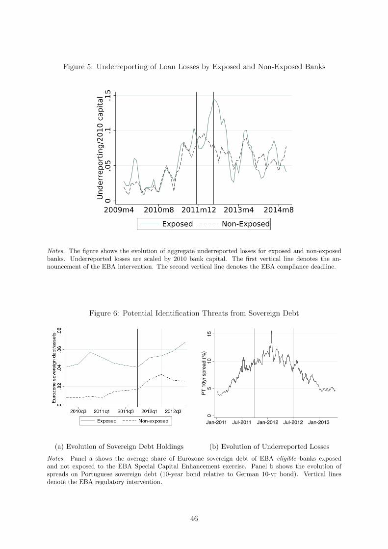
Figure 5: Underreporting of Loan Losses by Exposed and Non-Exposed Banks
0.0
5.1
.15
Und
erre
port
ing/
2010
cap
ital
2009m4 2010m8 2011m12 2013m4 2014m8
Exposed Non-Exposed
Notes. The figure shows the evolution of aggregate underreported losses for exposed and non-exposedbanks. Underreported losses are scaled by 2010 bank capital. The first vertical line denotes the an-nouncement of the EBA intervention. The second vertical line denotes the EBA compliance deadline.
Figure 6: Potential Identification Threats from Sovereign Debt
(a) Evolution of Sovereign Debt Holdings
05
1015
PT 1
0yr s
prea
d (%
)
Jan-2011 Jul-2011 Jan-2012 Jul-2012 Jan-2013
(b) Evolution of Underreported Losses
Notes. Panel a shows the average share of Eurozone sovereign debt of EBA eligible banks exposedand not exposed to the EBA Special Capital Enhancement exercise. Panel b shows the evolution ofspreads on Portuguese sovereign debt (10-year bond relative to German 10-yr bond). Vertical linesdenote the EBA regulatory intervention.
46

Figure 7: Firm-bank Credit Results-.0
6-.0
30
.03
.06
Trea
tmen
t effe
ct
2010Q2-Q42011Q1-Q3
EBABailout
2013Q2-Q4
All others Underreported
(a) Underreported firms
-.06
-.03
0.0
3.0
6Tr
eatm
ent e
ffect
2010Q2-Q42011Q1-Q3
EBABailout
2013Q2-Q4
All others Not underreported
(b) Non-underreported firms
Notes. The graphs shows results of the firm-bank level credit regression in specification 2, whichincludes firm×time and bank fixed effects as well as firm-bank-level controls. The dependent variableis the quarterly credit growth. We plot the coefficients on the two interactions periodτ × exposedb andperiodτ × underreportedib × exposedb, which are the respective treatment effects for the baseline groupof firms and the group of firms subject to loss underreporting. In panel b, we plot the triple interactionperiodτ × not underreportedib × exposedb, which are relationships with loan losses but which are notunderreported. Standard errors are clustered at the firm and bank level. The shaded area marks theperiod of the EBA intervention. See Table 12 in Appendix B for point estimates. N = 1,981,219.
Figure 8: Firm-level Credit Treatment Effects
-.1-.0
50
.05
.1Tr
eatm
ent e
ffect
2011Q12011Q3
2012Q12012Q3
2013Q12013Q3
All others Underreported
(a) Total Credit
-.1-.0
50
.05
.1Tr
eatm
ent e
ffect
2011Q12011Q3
2012Q12012Q3
2013Q12013Q3
All others Underreported
(b) Performing Credit
Notes. The graphs show results of the firm-level credit regression in specification 3. The dependentvariable is the quarterly log of total credit for a given firm in panel a and the quarterly log of performingcredit in panel b. We plot the coefficients on the two interactions quartert × treatmenti and quartert ×treatmenti × underreportedi, which are the treatment effects for the baseline group of firms, and thegroup of firms subject to loss underreporting. The shaded area marks the period of the EBA intervention.The specification includes the full set of interactions, industry×quarter and firm fixed effects, as wellas firm-level controls interacted with quarter. All coefficients should be interpreted as changes in thedependent variable relative to the (normalized) base quarter 2011Q3. Standard errors are clustered atthe firm-level. N= 1,346,771.
47

Figure 9: Correlations with Borrowing Share from Exposed Banks
assets
employees
sales gr
roa
leverage
current ratio
cash/assets
fix/assets
-.08 -.04 0 .04 .08Correlation (95% CI)
(a) Firm-level
loan size
share performing
rel length
firm share
main lender
bank share
-.08 -.04 0 .04 .08 .12Correlation (95% CI)
(b) Relationship-level
Notes. Panel a shows the correlation of normalized firm-level observables with the (normalized) firm-leveltreatment variable for the subset of firms subject to loss underreporting. Treatment is the borrowingshare from banks exposed to the EBA intervention. The correlations are conditional on 2-digit industryfixed effects and firm size buckets. All variables are averaged over 2008-2010. The right panel showsthe correlation of normalized relationship-level variables with a bank exposure dummy for the subset ofrelationships subject to loss underreporting. share performing refers to the share of total credit that isnot in default. rel length refers to relationship length. firm share refers to the share of the firm’s loanbalance in the bank’s loan portfolio. main lender is a dummy if the bank is the firm’s largest lender.bank share refers to the share of the bank in the firm’s loan portfolio.
48

For Online Publication: Appendix A1: A Method to
Detect the Underreporting of Loan Losses
Notation
We denote the observed loan balance reported in overdue bucket k in month t by Bib(t; k)where i denotes the firm and b the bank. We will drop the firm-bank subscripts in thediscussion that follows. There are 14 reporting buckets of overdue which correspond tothe overdue buckets in the regulatory schedule
k ∈ {{0} , {1} , {2} ., {3, 4, 5} , . . . , {30, . . . , 35}}
where 0 refers to loans overdue less than 30 days. We denote the set of available reportingbuckets by K. The first three buckets are monthly, thereafter we observe three-monthbuckets and thereafter 6-month buckets.
We also define a series of unobserved buckets c, which are defined at the monthlyfrequency c ∈ {{0} , {1} , {2} ., . . . , {35}} . We also define an unobserved amount of lend-ing C(t; c), which is the the loan balance in each of the unobserved monthly buckets.These underlying unobserved loan balances have to add up the observed distribution:B(t; k) =
∑c∈k C(t; c). We will exploit the fact that we can observe the first three
monthly buckets in the data, that is, we can observe C(t; c) for c ∈ {0, 1, 2}.We first assume that there are no inflows or outflows, with the exception of entry
mass IN(t; 0) = Cj(t; 0) that enters the system in the lowest reporting bucket. We relaxthis assumption in the following section. In the absence of any inflows and outflows, itmust hold that C(t; c) = C(t− 1; c− 1).
Intuitively, the loan balance we observe in bucket c at t must be the loan balance thathas moved up from the preceding bucket in the previous period. We define excess massas the deviation from this identity:
E(t; b) = C(t; c)− C(t− 1; c− 1). (11)
We also assume that excess mass occurs only at the upper edge of a bucket. Thatis, there is no incentive to delay moving up a reporting bucket before a loan reaches thehighest ‘sub-bucket’. Formally, these assumptions are:
1. C(t; c) = C(t− 1; c− 1), for all c with
min {k} < c < max {k} , for k with c ∈ k.2. C(t; c+ 1) + C(t; c) = C(t− 1; c) + C(t− 1; c− 1), for all c with
c = max {k} , for k with c ∈ k.
Baseline Algorithm
The goal of the algorithm is to compute the amount of excess mass in each reportedoverdue bucket k in each month t for each lending relationship.
49

We define the auxiliary concept of cumulative excess mass as
E(t; k) =s∑j=1
E(t− j; k). (12)
Cumulative excess mass is the excess mass accumulated in a bucket k over the past smonths where s denotes the length of the bucket (e.g. three months).
We proceed in two steps: We first calculate cumulative excess mass E(t; k) fromthe observed mass B(t; k), and then recursively calculate excess mass E(t; k) from thecumulative excess mass.
The algorithm consists of the following steps:
1. Set E(−1; k) = 0 = E(0; k) for all k ∈ K.
2. For all t = 1, . . . , T
(a) E(t; {0, 1, 2}) = B(t; {2})−B(t; {1}).(b) E(t; {0, 1, 2}) =
∑tτ=t−2E(τ ; {0, 1, 2}).
(c) For all k = 4, . . . , 8
i. Cumulative excess mass
E(t; k) = B(t; k)−B(t− 3; k − 1) + E(t; k − 1).
ii. Excess mass
E(t; k) = E(t; k)− E(t− 2; k)− E(t− 1; k).
(d) For k = 9
i.
E(t, k) = B(t; k)−B(t− 6; k − 1)−B(t− 6; k − 2)
+E(t, k − 1) + E(t− 3, k − 1) + E(t− 3, k − 2).
(e) For k = 10, . . . , K
i.
E(t, b) = B(t; k)−B(t− 6; k − 1) + E(t, k − 1).
ii.
E(t; k) = E(t; k)−5∑
τ=1
E(τ ; k).
We initialize the level of excess mass at zero in the month when our data is first available(January 2009) (step 1). For the first three buckets, we observe each month reportedseparately and hence directly use the baseline formula to calculate excess mass for thefirst bucket (step 2a). We here assume that excess mass will occur at the thresholdbetween bucket {2} and {3} since the deduction rate is constant across the first threebuckets. In step 2b, we obtain cumulative excess mass for the first combined three-monthbucket at t by adding the excess mass in the first combined three-month bucket acrossthe past three months. For the following buckets, we have to take into account that
50

reporting is done in buckets that stretch over three or six months respectively. We firstcompute cumulative excess mass in step i. by exploiting that the amount we observe inbucket k at time t is the sum of the amount that has been moved from the preceedingbucket k − 1 over the course of the last three months minus the cumulative excess massin the preceeding bucket that was not transferred over the last three months, plus thecumulative excess mass that has stayed behind in bucket k over the past three months.Once we have calculated excess mass in step i., we can then recursively compute excessmass in step ii. We repeat similar steps for the six-month buckets.
Algorithm with Flows
We now explain how to adjust the baseline algorithm for flows. We allow for the observedlending at t to be affected by time t inflows and outflows. The observed lending stockevolves as follows stockt = stockt−1 + net inflowt. We can further decompose net inflowsinto the following components
net inflowt = entryt + installmentst − written-offt − restructuredt + residualt.
Inflows, other than the initial entry inflow, consist of installments that fall overdue.Inflows into buckets higher than the initial k = 0 will lead us to overestimate excess masssince these flows add to the observed mass at t. Since installments tend to be of fixed sizeand occur at regular intervals, we classify an increase in the overdue loan balance thatcorresponds to an exact decrease in the balance of performing credit and that occurs atleast twice as an installment.
Outflows in contrast will lead us to underestimate excess mass since we subtract toomuch past mass. In the extreme case, this will lead us to obtain negative excess mass.Outflows happen for three reasons: repayment, restructuring and write-offs. If a bankrestructures or write offs an overdue loan, it reduces the overdue balance and increases therestructured/write-off balance which are separate entries in our data. We can thereforemeasure outflows into these two categories by a reduction in the overdue balance in agiven bucket that is less or equal to the change in restructured/written-off balance inthe same month. We cannot directly measure repayments of overdue loans which willinstead be recorded as a (negative) residual. We distribute the residual across bucketsby assigning the residual to the buckets with non-zero overdue balances in line with theshare of lending reported in that bucket.
Since this distribution of residual flows to buckets is somewhat arbitrary, we conductrobustness checks to see how much the results change when shifting the residual flows tothe lowest (highest) buckets. Since residual flows are small, the results are not affectedby this assumption (see Figure 11a in Appendix B).
The basic formula adjusted for flows is
E(t; k) = [C(t; c)− IN(t; c)]− [C(t− 1; c− 1)−OUT(t; c− 1)] . (13)
We subtract inflows out of bucket c since these flows contribute to observed mass butdo not contribute to excess mass. We add outflows from the preceding bucket sincewe do not expect these outflows to have moved up into the next reporting bucket. Ifwe observed only monthly buckets, then we could again apply the simple formula to all
51

buckets. However, for the three-month and six-month buckets, we again need to resortto the auxiliary concept of cumulative excess mass.
The formula for cumulative excess mass adjusted for flows is as follows:
E(t, k) = B(t; k)−B(t− 3; k − 1) + E(t, k − 1)
+ ˆOUT(t; k − 1)− IN(t; k − 1)− IN(t; k) + ˆOUT(t; k).
The flow adjustments consists of the following components. We denote individual monthlybuckets within each three-month bucket as k{1}, k{2}, k{3}. Hence k{2} refers to themiddle bucket within the three month bucket k.
1. ˆOUT(t; k − 1): For outflows, we want to subtract all outflows out of the precedingbucket over the past three months, which we would not have expected to have turnedup in the current bucket. Specifically, these are the outflows from the ‘boundary’bucket {3} that we would not expect to move across into the next bucket:
ˆOUT(t; k − 1) = OUT(t, (k − 1){3})+ OUT(t− 1, (k − 1){3}) + OUT(t− 2; (k − 1){3}).
2. IN(t; k − 1): There are inflows into the previous bucket k − 1, some of which weexpect to have moved by time t and we need to add:
IN(t; k − 1) = IN(t− 3; (k − 1){1})) + IN(t− 3; (k − 1){2})) + IN(t− 3; (k − 1){3}))︸ ︷︷ ︸already incorporated in B(t-3,k-1)
+ IN(t− 2; (k − 1){2}) + IN(t− 2; (k − 1){3})) + IN(t− 1; (k − 1){3})= IN(t− 2; (k − 1){2}) + IN(t− 2; (k − 1){3})) + IN(t− 1; (k − 1){3}).
3. IN(t; k): There are inflows into the current bucket k which we do not expect to havemoved up to the next reporting bucket so they need to be added. Note that outflowsonly affect how much moves on to the next bucket but not how much sticks around:
IN(t; k) = IN(t; k{1})) + IN(t; k{2})) + IN(t; k{3}))︸ ︷︷ ︸IN(t;k)
+ IN(t− 1; k{1}) + IN(t− 1; k{2})) + IN(t− 2; k{1}).
4. ˆOUT(t; k): Some of the mass that has moved up into the current bucket over thecourse of the past three months may have left the current bucket in the form ofoutflows, which we need to subtract. We only want to correct for the part thatcame in and then left again. So effectively we subtract the outflows from the bucketk from the inflow into bucket k. We cannot precisely tell which outflows exactlycorrespond to the inflows hence we just consider the total outflows. The earliestsuch outflow can occur at t − 1. Outflows at time t do not affect the measure ofexcess mass: ˆOUT(t; k) = OUT(t− 1, k) + OUT(t− 2; k).
We cannot measure the flows in and out of unobservable sub-buckets, which we de-noted by k{1}, k{2}, k{3}. Hence we have to approximate the flows that we definedabove by making an assumption how the total flow is distributed across the months that
52

comprise a given bucket. We can however specify the bounds for each flow componentand have an exact measure for the last. The bounds are as follows:
1. 0 ≤ ˆOUT(t; k − 1) ≤∑3
j=0 OUT(t− j; k − 1)
2. 0 ≤ IN(t; k − 1) ≤ IN(t− 1; k) + IN(t− 2; k)
3. IN(t; k) ≤ IN(t; k) ≤ IN(t; k) + IN(t− 1; k) + IN(t− 2; k)
4. ˆOUT(t; k) = OUT(t− 1, k) + OUT(t− 2; k)
Table 8: Effects of Assumptions on Flows
Total mass estimate ˆOUT(t; k − 1) IN(t; k) IN(t; k − 1)Effect on excess mass + − −Max Upper Lower LowerBaseline Upper Upper UpperMin Lower Upper Upper
Table 8 shows the combination of assumptions that generate the largest (and smallest)excess mass. For our baseline results, we choose the upper bounds for all flows whichis a middle ground between combinations that yield that largest and smallest resultsrespectively. In Figure 11a in Appendix B, we present results using the maximum andminimum combinations respectively. Figure 11b in Appendix B shows that the we getsimilar results when ignoring flows and simply using the formulas that only considerstocks. The reason is both that flows are small relative to stocks and that in manyinstances inflows and outflows cancel out.
The formulas above applied to three-month reporting buckets. The six-month bucketshave analogous formula.
Additional restrictions
We impose the following additional restrictions:
1. We impose that excess mass can never exceed observed mass in bucket.
2. We also impose that excess mass must be weakly positive since negative excess massis just a mis-measured outflow: B(t; k) ≤ 0.
3. We adjust for the common practice of banks to move overdue loans off their balancesheet in December to boost end-of-year statements, and putting the overdue balanceback on in January. This leads to spurious fluctuation in our measure of excess mass.
53

Appendix A2: Validity Checks for Algorithm
First validity test The first validity test regresses excess mass, the amount of under-reporting, at firm i, bank b, month t, collateral type c, and reporting bucket k on a set ofdummies that capture the increments in the mandatory deduction rate between reportingbucket k and k + 1:
excess massibkctoverdue loansibkct
=5∑j=1
βj∆deduction ratej + ϕb + θi + µt + εibkct. (14)
where i, b, c, k and t index firms, banks, collateral type, reporting category and month.We include firm-bank fixed effects and hence only use variation within a given lendingrelationship. We cluster standard errors at the firm-bank level. j indexes the possibleincrements in the regulatory rate, ranging from 0 to 25 percentage points (p.p.).
The coefficients βj measure the additional amount of excess mass that occurs in buck-ets when the change in the regulatory deduction rate from k and k+1 is equal to ∆ratej,relative to buckets where the regulatory rate stays constant. If banks act strategically,we would expect all coefficients to be positive and statistically significant, and larger rateincrements to have larger coefficients. We only consider relationships that have a singletype of collateral to avoid confounding the estimate by including relationships with sev-eral types of collateral since the regulatory rules differ by collateral type. We estimatethe specification separately for each type of collateral. Results are presented in Table 9and discussed in section 2.
Second validity check Since we can directly trace the time a loan has been overduein the subset of relationships with only a single loan, we can plot the average amountof underreporting against the actual overdue duration based on the data.60 We expectunderreporting to be most pronounced when the regulatory deduction rate increases asthis implies that banks continue to deduct at the lower rate associated with the previ-ous reporting bucket. For example, the regulatory rate increases when switching fromreporting that the loan has been overdue 5 months to reporting that is has been over-due 6 months. Hence the incentive to underreport is highest when the actual overdueduration has reached 6 months. By reporting that the 6-month overdue loan continuesto have been overdue only 5 months, the bank avoids the jump up in impairment lossesassociated with reporting 6 months. As in the first exercise we select the loans that haveonly a single type of collateral since the regulatory schedule differs by collateral type.Figure 10 provides visual evidence of ‘bunching’. In other words, the figures show spikesin the amount of underreporting just after an increase in the regulatory rate as we wouldexpect. Moreover, the spikes occur in different places for different collateral types in linewith differences in the regulatory rules.
We formally confirm the existence of bunching by regressing the amount of excessmass in month t on a categorical variable that captures the same set of increments in theregulatory deduction rate as above. Table 10 confirms that an increase in the regulatoryrate strongly correlates with an increase in the scaled amount of loss underreporting, orexcess mass. For example, an increase in the rate by 24 percentage points leads to an
60This exercise resembles the more traditional bunching graphs, which plot the cross-sectional distri-bution to provide a visual test for the presence of excess mass at the points where bunching is expectedto occur.
54

11 percentage point increase in the loan balance that is subject to loss underreporting(relative to the time periods without an increase in the regulatory rate). The effect is non-monotonic with larger increases for the 3-5 months reporting category, which correspondsto ∆ratet−1 = 9 for collateralized loans and ∆ratet−1 = 24 for non-collateralized loans.This non-monotonicity is due to the pressures to avoid classifying loans as non-performingexplained in section 2.
55

Table 9: Algorithm Validity Check:Bunching at Points of Rate Increases
Panel a: Bunching test(1) (2) (3)
Excess mass/loans No collateral Guarantee Real collateral
Increase in deduction rate innext higher reporting bucket9 p.p. 0.244 0.110
[0.002] [0.005]15 p.p. 0.451 0.349
[0.002] [0.004]24 p.p. 0.178
[0.005]25 p.p. 0.324 0.098 0.014
[0.005] [0.001] [0.002]N 363,132 1,253,589 232,659R2 0.581 0.450 0.464
Panel b: Placebo test
(1) (2) (3)Excess mass/loans No collateral Guarantee Real collateral
Increase in deduction rate innext higher reporting bucket25 p.p. -0.024 -0.004 -0.015
[0.001] [0.001] [0.001]N 363,132 1,253,589 232,659R2 0.199 0.213 0.224
Notes. The table shows regression results for the first validity test of the loss underreporting algorithm.The dependent variable is the amount of excess mass (or underreporting) scaled by the total overdueloan balance in a given reporting bucket for a firm-bank relationship (see table 1 for a visual depiction).The explanatory variables are a series of dummies that capture how much the regulatory deduction rateincreases from the current reporting bucket to the next higher reporting bucket (e.g. deduction rate of1% vs. 10% = increase of 9 p.p.). This difference measures the intensity of the incentive to underreport.The sample is split by collateral type since the regulatory rules differ by collateral type. Each columncorresponds to the results of a regression in the sample of firm-bank pairs that only have that type ofcollateral. The omitted baseline category is 0 (no rate increase). Hence the coefficients capture howmuch more excess mass (or underreporting) occurs in reporting buckets where there is an increase in theregulatory rate in the next higher bucket. Regressions include firm×bank fixed effects. The placebo testregresses underreporting on buckets where there is a rate increase for the other collateral type but notfor the given collateral type. Standard errors are clustered by firm-bank pair. No significance stars areshown.
56

Table 10: Loss Underreporting:Bunching in Sample of Single-Loan Relationships
Excess mass/loan balance (1) (2) (3)Increase in regulatoryrate between t− 1 and t9 p.p. 0.062 0.063 0.061
[0.008] [0.008] [0.008]15 p.p. 0.032 0.033 0.032
[0.007] [0.007] [0.007]24 p.p. 0.111 0.109 0.115
[0.018] [0.018] [0.021]25 p.p. 0.026 0.025 0.030
[0.004] [0.004] [0.004]Bank, firm FE Y Y NControls N Y NN 601,502 601,502 603,252R2 0.118 0.118 0.019
Notes. The table shows regression results for the second validity test of the loss underreporting algorithm.The dependent variable is the amount of excess mass scaled by the total loan balance in a given reportingbucket for a firm-bank relationship (see table 1 for a visual depiction). The explanatory variables area series of dummies that capture how much the regulatory deduction rate increases from the reportingbucket in month t-1 to the reporting bucket at t. t refers to the constructed time overdue (counting inthe data how long a loan has been overdue). The increase in the regulatory rate measures the intensity ofthe incentive to underreport. The sample only includes relationships with a single loan for which we canconstruct the time overdue. The omitted baseline category is 0 (no rate increase). Hence the coefficientscapture how much more excess mass (or underreporting) occurs in months where there is an increase inthe rate in the following month. Controls are the type of collateral. Standard errors are clustered byfirm-bank pair. No significance stars are shown.
Figure 10: Algorithm Validity Test for Single-loan Relationships
0.0
5.1
.15
Und
erre
port
ed lo
ss/lo
an v
olum
e
0 10 20 30Time overdue (months)
(a) Loans with Guarantee
0.0
5.1
.15
Und
erre
port
ed lo
ss/lo
an v
olum
e
0 10 20 30Time overdue (months)
(b) Loans without Collateral
0.0
5.1
.15
Und
erre
port
ed lo
ss/lo
an v
olum
e
0 10 20 30Time overdue (months)
(c) Loans with Real Collateral
Notes. The graph plots the average amount of underreporting against the actual time a loan has beenoverdue. We only consider single-loan relationships where we can track the actual time overdue (thenumber of months the bank has reported any positive overdue loan balance). The vertical lines denotethe points where we would expect most underreporting to occur (increase in the regulatory deductionrate). These points differ according type of collateral. We only consider loans with a single type ofcollateral.
57

For Online Publication: Appendix B: Additional Ta-
bles and Figures
Table 11: Additional Descriptive Statistics
Firm finance loans Undereported firms
Average Average Difference
Loan amount 269,729 Assets (m) 1.09 0.516(2x10⁶) (5.165) [0.041]
Fraction overdue 0.50 Leverage 0.205 0.097(0.42) (0.41) [0.004]
Fraction 0.73 EBIT/sales 0.13 0.009collateralized (0.44) 0.16 [0.002]Fraction w/ 0.79 Debt/EBITDA -0.300 -0.771guarantee (0.41) (12.911) [0.066]Fraction w/ real 0.32 EBITDA/assets -0.052 0.011collateral (0.47) (0.292) [0.002]Maturity < 1yr 0.23 Sales growth -0.030 -0.018
(0.42) (0.709) [0.003]Resid maturity < 1yr 0.48 Cash/assets 0.053 -0.019
(0.50) (0.151) [0.001]Debt to government/assets 0.089 0.051
(0.135) [0.002]Collateral ratio 0.02 -0.039
0.17 [0.002]N 1,332,435 18,314
Notes. The left panel shows descriptive statistics at the loan-level for firm finance loans that have anoverdue loan balance at some point over their lifetime. This is the sample of loans on which we run thealgorithm to detect the underreporting of loan losses. The first column of the right panel shows descriptivestatistics for firms that are subject to loss underreporting in a given year. The second column of the rightpanel shows differences in means relative to firms that have overdue loans but are not underreported.The collateral ratio combines the extensive margin (has any collateral) and the intensive margin (valueof collateral). Standard errors in parentheses.
58

Tab
le12
:R
egre
ssio
nR
esult
sF
irm
-Ban
kL
evel
:In
tensi
veM
argi
n
Gro
wth
rate
ofcr
edit
(1)
(2)
(3)
(4)
(5)
(6)
Tota
lcr
edit
Per
form
ing
Non
-per
fN
ewlo
an
Pre
1 t×
exp
osedb
-0.0
11
-0.0
10
-0.0
11
-0.0
00
-0.0
24
[0.0
08]
[0.0
10]
[0.0
08]
[0.0
02]
[0.0
15]
Pre
2 t×
exp
osedb
-0.0
03
-0.0
05
-0.0
03
-0.0
00
-0.0
22
[0.0
10]
[0.0
10]
[0.0
10]
[0.0
02]
[0.0
14]
EB
At×
exp
osedb
-0.0
20
-0.0
22
-0.0
22
0.0
01
-0.0
39
[0.0
10]
[0.0
13]
[0.0
09]
[0.0
02]
[0.0
14]
Bai
lou
t t×
exp
osedb
-0.0
06
-0.0
08
-0.0
04
-0.0
02
-0.0
13
[0.0
06]
[0.0
08]
[0.0
07]
[0.0
03]
[0.0
11]
Pos
tb
ailo
ut t×
exp
osedb
0.0
08
0.0
06
0.0
09
-0.0
02
0.0
04
[0.0
08]
[0.0
12]
[0.0
09]
[0.0
02]
[0.0
11]
Pre
1 t×
exp
osedb×
un
der
rep
orte
dib
0.0
08
0.0
01
0.0
18
0.0
07
-0.0
06
0.0
09
[0.0
13]
[0.0
13]
[0.0
12]
[0.0
13]
[0.0
07]
[0.0
08]
Pre
2 t×
exp
osedb×
un
der
rep
orte
dib
0.0
08
0.0
06
0.0
21
0.0
10
-0.0
04
0.0
16
[0.0
23]
[0.0
23]
[0.0
25]
[0.0
20]
[0.0
07]
[0.0
23]
EB
At×
exp
osedb×
un
der
rep
orte
dib
0.0
41
0.0
44
0.0
50
0.0
38
0.0
05
0.0
69
[0.0
13]
[0.0
12]
[0.0
19]
[0.0
15]
[0.0
09]
[0.0
22]
Bai
lou
t t×
exp
osedb×
un
der
rep
orte
dib
0.0
19
0.0
27
0.0
27
0.0
35
-0.0
08
0.0
42
[0.0
19]
[0.0
16]
[0.0
19]
[0.0
15]
[0.0
11]
[0.0
17]
Pos
tb
ailo
ut t×
exp
osedb×
un
der
rep
orte
dib
0.0
05
0.0
16
0.0
23
0.0
22
-0.0
07
0.0
30
[0.0
14]
[0.0
11]
[0.0
13]
[0.0
14]
[0.0
10]
[0.0
12]
Ban
k×
qu
arte
rF
EY
NN
NN
NF
irm×
qu
arte
rF
EY
YN
YY
YF
irm
,qu
arte
rF
EN
NY
NN
NN
1,9
81,2
19
1,9
81,2
19
1,9
81,2
19
1,9
81,2
19
1,9
81,2
19
1,9
81,2
19
R2
0.3
81
0.3
79
0.0
57
0.3
83
0.4
05
0.4
13
Ban
ks
45
45
45
45
45
45
Notes.
Th
eta
ble
show
scr
edit
regr
essi
ons
resu
lts
atth
efi
rm-b
an
kle
vel.
Th
ed
epen
den
tva
riab
leis
the
qu
art
erly
gro
wth
rate
into
tal
cred
itfo
ra
giv
enfi
rm-b
an
kp
air
inco
lum
ns
(1)-
(5).
Col
um
ns
(4)
and
(5)
dec
omp
ose
tota
lcr
edit
gro
wth
into
per
form
ing
an
dn
on
-per
form
ing
cred
it.
Th
ese
gro
wth
rate
sare
defi
ned
as
the
qu
arte
rly
chan
ges
scal
edby
lagg
edto
tal
cred
it.
For
exam
ple
,th
egro
wth
rate
inp
erfo
rmin
gcr
edit
isd
efin
edas
∆cperf
ibt/callib,t−1.
Colu
mn
6p
rese
nts
resu
lts
from
ali
nea
rp
rob
abil
ity
mod
elw
her
eth
ed
epen
den
tva
riab
leis
ad
um
my
that
is1
ifth
enu
mb
erof
loan
sin
afi
rm-b
an
kp
air
incr
ease
s(c
on
dit
ion
al
on
an
incr
ease
inlo
anvo
lum
e).
Th
eex
pla
nat
ory
vari
able
exp
osed
isa
du
mm
yth
at
is1
for
ban
ks
exp
ose
dto
the
EB
Ash
ock
.T
he
sam
ple
per
iod
is2009q1-2
014q4.
Pre
1an
d2,
EB
A,
bai
lou
tan
dp
ost-
bai
lou
tar
ed
um
mie
sth
atid
enti
fyth
efo
llow
ing
tim
ep
erio
ds:
the
EB
Ain
terv
enti
on
(2011q4-2
012q2),
the
bail
ou
tp
erio
d(2
012q-2
012q4),
two
pre
-per
iods
and
one
pos
t-b
ailo
ut
per
iod
all
ofeq
ual
len
gth
.U
nd
erre
port
edis
afi
rm-b
an
kd
um
my
that
iden
tifi
esre
lati
on
ship
ssu
bje
ctto
loss
un
der
rep
ort
ing
inth
efo
ur
qu
arte
rsp
rior
toth
eE
BA
shock
.A
llre
gres
sion
sin
clu
de
ban
kfi
xed
effec
tsan
dfi
rm-b
an
kco
ntr
ols
(see
text
for
det
ails)
.S
tan
dard
erro
rsin
pare
nth
eses
and
are
two-
way
clu
ster
edby
ban
kan
dfi
rm.
Ad
dit
ion
alin
tera
ctio
neff
ects
are
om
itte
d.
See
equati
on
sin
sect
ion
3fo
rd
etail
son
full
set
of
inte
ract
ion
effec
tsin
clu
ded
.S
ign
ifica
nce
star
sar
en
otsh
own
.
59

Table 13: Regression Results Firm-Bank Level: Robustness Checks
Growth rate of total credit (1) (2) (3) (4)
Pre1t×exposedb -0.009 -0.009 -0.016 -0.011[0.008] [0.011] [0.009] [0.009]
Pre2t×exposedb -0.004 -0.002 -0.018 -0.004[0.010] [0.010] [0.011] [0.011]
EBAt×exposedb -0.022 -0.020 -0.029 -0.022[0.010] [0.013] [0.011] [0.010]
Bailoutt×exposedb -0.009 -0.005 -0.015 -0.009[0.006] [0.006] [0.008] [0.006]
Post bailoutt×exposedb 0.006 0.008 0.002 0.008[0.007] [0.012] [0.009] [0.008]
Pre1t×exposedb×underreportedib 0.002 0.012 0.013 0.001[0.013] [0.010] [0.008] [0.013]
Pre2t×exposedb×underreportedib 0.006 0.024 0.012 0.006[0.023] [0.023] [0.016] [0.023]
EBAt×exposedb×underreportedib 0.043 0.051 0.051 0.044[0.013] [0.017] [0.015] [0.012]
Bailoutt×exposedb×underreportedib 0.027 0.026 0.034 0.027[0.017] [0.021] [0.010] [0.016]
Post bailoutt×exposedb×underreportedib 0.016 0.021 0.014 0.011[0.012] [0.014] [0.010] [0.009]
Firm×quarter FE Y N N YFirm, quarter FE N Y Y NRelationship controls N Y Y YFirm-level controls N Y N NN 1,981,219 1,859,321 5,244,714 1,981,219R2 0.378 0.057 0.069 0.417Banks 45 45 45 45
Notes. The table shows additional credit regressions results at the firm-bank level for the intensivemargin. The dependent variable is the quarterly growth rate in total credit for a given firm-bank pair.The explanatory variable exposed is a dummy that is 1 for banks exposed to the EBA shock. SeeTable 12 for additional details. Relative to column 2 of Table 12, column 1 omits our baseline controls,column 2 adds additional firm-level controls (ebitda/assets, leverage, sales growth - all interacted withthe period dummies), column 3 clusters standard errors at the bank-level, and column 4 adds control forthe bank-level use of the LTRO program. No significance stars are shown.
60

Table 14: Regression Results Firm-bank Level:Extensive Margin
Pr(relationship cut) (1) (2) (3)
EBAt×exposedb 0.057 0.056 0.058[0.011] [0.011] [0.012]
Bailoutt×exposedb 0.041 0.042 0.043[0.009] [0.008] [0.008]
Post bailoutt×exposedb 0.029 0.030 0.029[0.010] [0.009] [0.009]
EBAt×exposedb×underreportedib -0.217 -0.202 -0.219[0.034] [0.027] [0.057]
Bailoutt×exposedb×underreportedib -0.106 -0.090 -0.105[0.033] [0.030] [0.047]
Post bailoutt×exposedb×underreportedib -0.053 -0.041 -0.050[0.018] [0.015] [0.024]
Firm FE Y N YFirm controls N Y NN 2,973,566 2,538,082 2,973,566R2 0.706 0.137 0.706Banks 46 45 46
Notes. The table shows credit regressions results at the firm-bank level for the extensive margin (linearprobability model). The dependent variable is a dummy that turns one when the relationship is cut,defined by the performing loan balance dropping to zero. The explanatory variable exposed is a dummythat is 1 for banks exposed to the EBA shock. Pre period 1 and 2, EBA, bailout and post-bailout aredummies that identify the following time periods: The EBA shock (2011q4-2012q2), the bailout period(2012q-2012q4), and one post-bailout period all of equal length. We cannot estimate pre-trends in thisregression since we condition on a sample of relationships that have positive loan balances in the pre-periods. underreported is a dummy that identifies relationships subject to underreported losses in thefour quarters prior to the EBA shock. All regressions include bank and quarter fixed effects. Column 1and 3 contain firm fixed effects. Column 2 includes industry×quarter fixed effects and firm-level salesgrowth and leverage interacted with the time period to allow for flexible time trends. Standard errorsin parentheses and are two-way clustered by bank and firm. Additional interaction effects are omitted.See equation 2 in section 3 for details on full set of interaction effects included. No significance stars areshown.
61

Table 15: Employment and Investment Results: Persistence and Placebo Tests
(1) (2) (3) (4) (5)
Growth rate Employees2013 2014 2011 2009 2008
∆ log crediti -0.555 3.326 -0.028 -0.653 0.102[0.218] [6.853] [0.045] [0.978] [0.074]
Controls Y Y Y Y YIndustry, size FE Y Y Y Y YFirst stage F-statistic 8.8 0.277 116.7 1.5 6N 105,170 93,729 126,595 126,595 124,478
Notes. The table shows IV regression results at the annual firm-level for different years. The dependentvariable is the symmetric growth rate of employment, which is a second order approximation to the logdifference growth rate and incorporates observations that turn to 0 (firm exit). We instrument for thelog change in credit using the (normalized) firm-level borrowing share from banks exposed to the EBAshock prior to the shock. Relative to Table 3, we only vary the year of the dependent and independentvariables. Controls consist of firm-size and 2-digit industry FE, as well as firm-level log total assets,interest/ebitda, capital/assets, currrent ratio, cash/assets and sales growth all averaged over 2008-2010.Lag refers to the lag of the dependent variable. Standard errors are clustered by industry. No significancestars are shown.
62

Figure 11: Robustness Checks on Algorithm2.
00e+
084.
00e+
086.
00e+
08Ex
cess
Mas
s
2009m12010m12011m12012m1 2013m12014m12015m12016m1
Residual in min bucket Residual in max bucketFlows: upper bound Flows: lower bound
(a) Robustness of Algorithm0
.005
.01
.015
.02
Exce
ss m
ass/
loan
vol
ume
0-23-5
6-89-11
12-1415-17
18-2324-29
30-36
No inflow correction Inflow correction
(b) Underreporting by Reporting Buckets
Notes. Panel a shows the aggregate amount of excess mass when varying different assumptions. Thefirst two lines show the results when we allocate residual flows to the lowest (highest) reporting bucket.The remaining lines show the effect of choosing the bounds on flows such that they have the minimum(maximum) impact on excess mass. Panel b h shows the distribution of excess mass (or underreporting)across reporting buckets. We scale the amount of excess mass by the total loan balance of that firm-bank pair. We compare the results of the algorithm with and without incorporating the effects of flows(repayments, new installments falling overdue, debt write-offs or restructuring) in the data.
Figure 12: Decomposition of Underreported Losses by Mechanism
0.2
.4.6
Frac
tion
2009m7 2011m1 2012m7 2014m1 2015m7
Excess length SwapsExcess length - same amount
Notes. The graph shows the decomposition of underreported losses by the mechanisms discussed insection 2. Excess length refers to spells of overdue reporting in a bucket that exceed the permissiblelength (e.g. loan reported to be overdue 3-5 months for 4 months in a row.). Excess length - same amountrefers to spells that exceed the permissible length where the loan balance does not change. Swaps refer tocases where there is a decrease in the overdue balance equal to an increase in the performing loan balance.This captures the last mechanism where banks grant new credit in exchange for the firm repaying thelongest overdue credit portion. All numbers are scaled by the total amount of excess mass.
63

Figure 13: Long-run Trends: Underreported vs Non-underreported Firms
0.0
5.1
.15
.2.2
5Pr
ob(e
xit)
0 2 4 6 8 10Year since first default
UnderreportedNot underreported
(a) Probability of exit
-.2-.1
0.1
Shar
e ov
erdu
e
0 2 4 6 8 10Year since first default
UnderreportedNot underreported
(b) Share of loans overdue
-.02
-.01
0Re
turn
on
asse
ts
0 2 4 6 8 10Year since first default
UnderreportedNot underreported
(c) Return on assets
-.15
-.1-.0
50
.05
Sale
s gr
owth
0 2 4 6 8 10Year since first default
UnderreportedNot underreported
(d) Sales growth
Notes. The graphs show the average evolution of firm-level measures over time. We plot the 95 confidenceintervals of the residualized mean for each group. The variables are residualized on year×industry fixedeffects and firm size. The x-axis are years following the first time we observe an overdue loan in the data(for a given firm). The upwards trend in sales is likely due to a survivorship bias since firms that exitdrop out of the sample.
64

Figure 14: Liquidity and Credit Pre-trends
-.4-.2
0.2
.4Co
effic
ient
2007 2008 2009 2010
(a) Current Ratio
-.005
0.0
05.0
1Co
effic
ient
2007 2008 2009 2010
(b) Cash/Assets
Notes. Panels a and b show results from a dynamic differences-in-differences specification where weinteract the firm-level borrowing share from banks exposed to the EBA shock with year dummies forthe period prior to the EBA shock. We run the regression in the subset of firms subject to loss under-reporting. The two panels show two different liquidity measures. Standard errors are clustered at thefirm-level.
Figure 15: Additional Results: Firm-level Regression
-.06
-.03
0.0
3.0
6Tr
eatm
ent e
ffect
2010Q2-Q42011Q1-Q3
EBABailout
2013Q2-Q4
Performing Non-Performing
Notes. The graphs show regression results at the quarterly firm-level. The dependent variables arethe quarterly log of performing and non-performing credit, respectively. We plot the coefficients onthe interaction treatmenti×quartert×underreportedi, which are the treatment effects for the group offirms subject to loss underreporting. The vertical lines denote the EBA announcement and compliancedeadline. The specification, equation 3, includes the full set of interactions, industry×quarter and firmfixed effects, as well as firm-level controls interacted with quarter. All coefficients should be interpretedas changes in the dependent variable relative to the (normalized) base quarter 2011Q3. Standard errorsare clustered at the firm-level. N= 1,346,771.
65

Appendix C: Estimating Production Functions
In order to compute the aggregate productivity decomposition in section 4, we need to es-timate firm-level technical efficiency as well as output elasticities. We use two approachesto obtain output elasticities. First, we compute 3-digit industry-level cost shares follow-ing Nishida et al. (2017) and Bollard et al. (2013). Second, we estimate the followingCobb-Douglas revenue production function at the annual firm level:
qit = βllit + βkkit + βmmit + βssit + εit. (15)
where i indexes firms and t years. qit is the log of real output, lit is the log of the numberof employees, mit is the log of real intermediate materials, and sit is the log of real servicesused by firm i in year t. We estimate the production separately for each 2-digit industrylevel, and for each 3-digit level for manufacturing firms. We winsorize all variables at the1% level prior to taking logs.
We obtain real output by deflating firm revenue by a 2-digit industry price index,which we obtain from the Portuguese statistics office (three digit for certain manufactur-ing industries). For non-manufacturing industries for which no price index is available,we use alternative deflators at the 2-digit level depending on the type of industry (agri-cultural price deflator, consumer price index, or services price index from Eurostat). Weobtain the real value of intermediate materials by deflating the cost of materials by amaterial input deflator from Eurostat, and proceed similarly for services. We adjustmaterials for the change in inventories.
We measure capital in two ways. We either use the deflated book value of fixed assetsor the perpetual inventory method. The latter is computed as follows. We deflate thestock of fixed assets in 2006 (or the earliest available firm-level observation) by the 2006capital goods deflator. We then compute the firm-level change in real fixed assets byadjusting lagged real fixed assets by the firm-level depreciation rate and adding firm-levelinvestment spending according to the following formula:
kit = (1− δit)kt−1 +
(Iitdeft
).
From 2009 onwards, we use CAPEX reported in the cash-flow statement when available(which is expenditure on tangible and intangible investment). Before 2009, or whenCAPEX is not reported, we simply use the change in the book value of fixed assets. Wedeflate investment spending by the capital goods deflator.
We calculate firm-level log TFP based on the gross output function as
logAit = qit −(βllit + βkkit + βmmit + βssit
)(16)
where we either use the coefficients based on cost shares, or our estimated coefficients.Our baseline estimates follow Wooldridge (2009). For robustness, we run two fur-
ther production functions estimations. We estimate the same specification but withfirm×period fixed effects, where the periods are 2005-2008, 2009-2012, 2013-2015. Wealso employ a translog specification, where we relax the Cobb-Douglas restrictions thatthe elasticities of ouptut are constant and the elasticity of substitution between inputs is
66

one. The translog specification is given by
qit =∑j
βjXjit + βjjX
j2
it +∑
j 6= k∑k
βjkXjitX
kit + εit. (17)
In Table 16 we provide the average estimated elasticities for all three methods. Wedrop all observations where the coefficients are negative, zero or missing. Our estimatesappear reasonable as the average sum of elasticities is close to 1 suggesting constantreturns to scale.
Table 16: Production Function Coefficient Estimates
Fixed assets Inventory methodCost shares Wooldridge Translog OLS Wooldridge Translog OLS
Sum 1.16 0.93 1.10 1.05 1.13 1.10 1.10(0.33) (0.53) (0.66) (0.33) (0.48) (0.57) (0.25)
Materials 0.33 0.32 0.35 0.29 0.32 0.34 0.280.26 (0.19) (0.35) (0.11) (0.20) (0.34) (0.12)
Services 0.32 0.59 0.53 0.46 0.69 0.52 0.450.2 (0.25) (0.24) (0.11) (0.38) (0.25) (0.12)
Employees 0.24 0.31 0.38 0.38 0.31 0.37 0.37(0.17) (0.19) (0.30) (0.13) (0.18) (0.23) (0.12)
Capital 0.28 0.02 0.04 0.02 0.04 0.05 0.04(0.27) (0.02) (0.07) (0.02) (0.03) (0.06) (0.02)
N 785 2590 2590 2590 2590 2590 2590
Notes. The table shows production function coefficients estimates. The first column shows coefficientsbased on 3-digit industry cost shares. The remaining columns are based on a gross output (revenuedeflated by industry deflators) Cobb-Douglas production function specifications. We show averagesacross industry-level coefficients and standard errors in parentheses. Wooldridge refers to the Wooldridge(2009) methodology. OLS and translog specification refer to a OLS version adding fixed effects and atranslog specification (following Petrin and Sivadasan (2013)). Fixed assets refers to the deflated bookvalue of fixed assets to measure capital while the inventory method uses the perpetual inventory methodto compute the real capital stock (see text for details).
67


![Shei Aloukik Imon - Sudipto Mukhopadhyay [Pbands] (1)](https://img.pdfslide.net/doc/110x75/577cc0821a28aba711905f63/shei-aloukik-imon-sudipto-mukhopadhyay-pbands-1.jpg)