Which are the world's wobblier currencies? Reference exchange

Which are the world’s wobblier currencies? Reference exchange rates and their variation

by Roger Bowden and Jennifer Zhu*

Abstract

Measuring country exchange rates relative to a common reference basket results in a set of no-arbitrage prices, unlike trade-weighted indexes, the usual method of comparing country exchange rate histories. The reference basket is analogous to a portfolio, and its choice can be resolved by drawing on required economic interpretations or uses. We use currency reference rates to examine the historical variability of different currencies over designated cyclical bands. The temporal decompositions used are those provided by wavelet analysis, which is light on maintained assumptions about data generating processes. Some countries, notably Japan and New Zealand do exhibit a powerful but irregular medium term cycle, while others are much more stable. Implications are briefly examined for investment, hedging, monetary policy and common currency studies. Key words: Currency volatility, reference exchange rates, reference basket,

spectral utility function, wavelets. JEL reference numbers: C19, C22, F31. * The authors are both with the School of Economics and Finance, Victoria University of Wellington, P.O. Box 600 Wellington New Zealand; emails [email protected] , [email protected] . Thanks for useful feedback go to seminar participants at the NZ Treasury, in May 2006.

1

1. Introduction Knowing whether currency A is more variable than currency B, or than other world

currencies, is an object of concern to investors, central bankers and policy makers, and to

corporations faced with purchase or location decisions. The idea that currencies might

differ in this respect is simple enough, but measurement turns out to be surprisingly

difficult. One has to resolve two sets of problems, the absolute exchange rate problem and

the variability horizon problem – long, medium or short run.

The first issue concerns the necessity to isolate the currency values for a particular

country. Exchange rates are inherently bilateral, yet we need to form a judgement about

this or that currency in isolation. Is the Japanese yen inherently more variable than the US

dollar or the UK pound? To answer that, we need an absolute rate for the Japanese yen,

the US dollar or the UK pound, to be extracted from the bilateral exchange rates between

them and possibly other currencies. But any exchange rate always has to be a relative

price, the price of one thing in terms of another, so that there is really no such thing as an

absolute exchange rate. The respective trade weighted index (TWI) are commonly used to

resolve such issues. The difficulty is that TWI’s cannot be reconstructed into bilateral

exchange rates, at least without arbitrage being possible. Thus the TWI’s are not

transactionally consistent with one another. Alternatively one could set the required

absolute country rates just as the bilateral rates against US dollar, as the international base

for currency no-arbitrage. This is indeed a valid choice, but it leaves the absolute rate for

the US dollar as unity and constant over time, apparently the very model of stability. Or

one could choose the country with the minimum rate of inflation and use its currency as

the base. But a moment’s reflection will show that low inflation is often the product of

monetary policies that incidentally create rather unstable currencies; New Zealand is a

case in point.

No-arbitrage absolute rates, in the desired sense, can be constructed by replacing a

single numeraire currency with a reference basket of world currencies, and measuring

each bilateral exchange rate relative to this basket. In constructing such currency

reference rates (CRR’s) there always remains one degree of freedom, which effectively

reduces to the choice of reference base. All no-arbitrage reference rates can be

constructed in this way. There is considerable freedom in the choice of reference bases,

indeed some of the weights be negative as well as positive, and there are useful analogies

with portfolio analysis. The reference base construction needs to be resolved in an

2

economically meaningful way, depending on the context and use. We suggest several

alternatives, each with its own shade of meaning.

The first is based on a simple geometric average of the bilateral rates, which turns

out to have a minimum norm property, namely that it minimises the distance between

country rates. A reference basket of this sort can be viewed as analogous to the use of a

minimum variance portfolio of currencies as benchmark. It is probably the simplest way

to approach arguments about whether this or that currency has been more variable than

another; construct an artificial currency as stable as possible, then see if the subject

currency is more variable. The centred rate, as we call it, is very easy to compute, and it

can conveniently serve as a point of departure for any other alternative base rate system.

A second alternative is to bias the reference basket in one way or another, notably

to conform with the trade or capital flows of a particular country of concern. The

reference basket has to remain common, to avoid arbitrage. But the interpretation

correspondingly changes. It is less concerned with issues as to which is the most variable

currency and becomes more particular to the concerns of a specific country of choice. The

apparent rates, as they are now called, are seen through the eyes of residents of the chosen

country. Suppose other countries had exactly the same trade or capital flow patterns as us:

would their currencies be as stable or unstable as ours relative to that reference base? This

is a possible window into common currency studies. In terms of the illustration, if New

Zealand had been operating off the Australian dollar, but unchanged trade weights, would

it have enjoyed or more or a less volatile exchange rate history?

Other alternatives are to base spot reference rate baskets on a single set of global

trade or capital weights, in effect some weighted average of each country’s own trade or

capital weights. An alternative starting point is to base the reference basket not on

nominal exchange rates, but real exchange rates or on forward exchange rate premiums.

A second set of problems concern the measurement of variation. This sort of issue

is hardly a problem if one believes that exchange rates follow a random walk, with or

without drift. But (as our methodology confirms), exchange rates over longer time

intervals have not, on the historical evidence, followed random walks. Some of the

country reference rates exhibit a quite pronounced cyclical character, even if it is not the

regularity demanded by standard (Fourier) spectral analysis. But cyclical or not, is there a

sense in which one can say that this or that absolute rate is more variable over a certain

horizon: the 5-6 year band of the business cycle, or the 1-2 year band or shorter? We

answer this and related questions by using wavelet analysis. This is a case of new wine in

3

old bottles. Originally called wave packets in quantum physics, the effective empirical

implementation for general use is much more recent. Wavelets cater for cycles of

irregular form or amplitude, as well as a more natural treatment of the trend-cycle

dichotomy. Wavelet analysis is easy on maintained assumptions about linearity or

nonlinearity, stationarity or nonstationarity, or as to implicit structural theorising. The

orthogonal decompositions that result enable a very simple approach to the issue of

variation over different horizons. Using it we can show that countries have differed in

their absolute exchange rate behaviour and that some have had more pronounced

variation than others, especially in certain cyclical bands. The latter finding has

importance for risk management and economic policy. Hedging is easy for short run

fluctuations but not so easy for the longer run, and the problem is more serious when high

amplitude cycles are present, but of irregular periodicity.

It should be stressed at the outset that currency variability is not an unequivocally

bad thing. A variable currency can smooth trade and other shocks, or can represent a

needed adjustment to structural changes. A finding that a country’s currency has exhibited

a lot of variability is one that needs to be examined on its own merits. Issues of this kind

are also briefly canvassed in the course of the present paper.

The scheme of the paper is as follows. Section 2 develops the reference currency

rate normalisations and their interpretation on a general level. Section 3 exposits the

essentials of wavelet analysis, with more detailed or technical material relegated to an

appendix. Section 4 applies these methods to a set of world currencies, in both nominal

and real terms, and with alternative normalisations, interpreting the results. Section 5

concludes, setting the results in the context of debates about risk management,

investment, economic policy and common currency debates.

2. Construction and use of reference currency rates As earlier noted, use of trade-weighted indexes is a common way of isolating a country’s

specific or intrinsic exchange rate. However trade or capital-weighted indexes have two

problems: First, they refer to only a subset of foreign exchange activities. For some

countries, trade flows account for a minor proportion of transactions, the bulk of the trade

being driven by capital transactions. More importantly, trade weighted indices have no

exchange content. Thus if TWIiA is the TWI index for country i, and TWI

jA that for country

4

j, one might think of constructing a bilateral exchange rate as TWIj

TWIi

TWIij AAR /= . But

this will differ from the actual traded rates ijR by a log linear function of the difference

between the TWI weights of the two countries. Any trader who tried to price actual

bilateral rates against TWI rates would not last very long. One would also want variation

in currencies to take full account of their pricing interdependence – only actual traded

prices do this properly.

A little structure is useful at this point; what follows is informal in nature with

more explicit proofs given in Appendix A. Let ijR be a bilateral exchange rate with

currency i as commodity currency and country j as terms currency, so that 1 country i unit

is worth ijR units of currency. Write ijij Rs log= and let njisS ij ,...1,));(( == be the

matrix of bilateral log exchange rates. Ignoring bid ask spreads, no-arbitrage will ensure

the existence of a set of country-specific prices Ai, or currency reference rates, such that

jiijj

iij aas

AA

R −== ; , where the a’s are the logs. For n currencies there are only (n-1)

independent reference rates1, so there is one degree of freedom in choosing them.

A simple way of constructing a set of mutually consistent currency reference rates

(CRR’s) is to take the bilateral rates with respect to a chosen numeraire currency, notably

the US dollar. This is how the market avoids arbitrages in practice. If the US is country n,

we would be taking the n’th column of S, as the vector of CRR’s, namely nsa = . Such a

choice has the advantage that adding another country to the set will not disturb the

existing CRR’s for the other countries. But it is not convenient in other respects, one of

which is that the numeraire country automatically has zero for its absolute (log) exchange

rate .One cannot easily compare the variation of currency n with that of the others.

Alternatively, we could choose for the currency reference rates any weighted

combination of the columns of S, of the form

∑∑ === j

jn

jjj

w ww 1;1

sa . (2.1)

Choosing currency n (e.g. the US dollar) as base would amount to setting nsa = , which

in turn is equivalent to setting new = the nth column of the identity matrix. A more

general choice is

5

nnwww eeew +++= ...2211 ; 1=∑j

jw . (2.2)

One is now replacing a single currency as the numeraire with a basket of world currencies

with weights given by the vector w .We could call this a ‘reference basket’ or ‘reference

basis’ for the system. The CRR wia for country i is the bilateral rate for that currency with

respect to the reference basket, viewed as though it was a currency in its own right.

In fact, all no-arbitrage CRR vectors can be constructed in this way, i.e. as some

weighted average of the bilateral rates as in expression (2.1). There is no particular need

to have all weights wi semipositive – it is quite possible to think of a reference basis that

is short in some currencies and long in others, rather like a portfolio, with which problem

it has some features in common2. Because the matrix S of log bilateral rates has to be

skew symmetric 0' =ww S , from which it follows that ∑ =j

jwj wa 0 . This looks rather

like a system balance of payments condition where the commodities being bought or sold

in quantities wj are the currencies at their respective prices aj . In fact, it is just a

requirement that the bilateral rate of the reference base against itself has to be zero.

The problem then boils down to the best choice of the reference basket w for the

intended purpose. Some leading candidates are canvassed in what follows.

2.1 Centred rates

A simple choice is to set n

w j1= , all j. The reference basket is a simple average of the

world currencies, so that no single country is singled out for special weight. The resulting

CRR vector is given by

1a Sn10 = , (2.3)

where 1 denotes the unit vector ( all elements =1). This is the simple average of the

bilateral rates. The intuition is that taking an equally weighted basket creates a stable

portfolio of currencies, so one might as well measure the variation of the individual

currencies relative to a stable base. One can call the resulting CRR’s the ‘centred rates’,

for if a is any other CRR vector, then aaa ii += 0 , which means that any alternative CRR

can always be represented as the centred CRR plus a common factor that adjusts for the

mean.

6

The centred rates a0 have a minimum Euclidean norm property: among all

qualifying CRR’s, they minimise the length aa' . This is useful if one wants to be

conservative in judgements that currencies exhibit divergent behaviour – make sure that

they are as similar as possible to begin with. The minimum norm property extends to the

covariance matrix Ωa of the CRR’s, assuming it exists: all other choices a have a higher

trace norm than does the centred version a0 (see the remark in Appendix A). Thus the

centred version can be regarded as minimising the average variation in the system.

The centred version is also useful as a point of departure for other possible

reference bases. Indeed one can write

1awaa )'( 00 −= . (2.4)

The term 0'aw adjusts to the new base weights w. The two CRR’s will differ to the extent

that the value of the basket w at the centred CRR’s is non zero. Actually, an expression of

the general form (2.4) applies to conversion between any CRR systems. For instance one

could replace a0 on the right hand side with the CRR’s based on the US dollar as the

reference basis; formula (2.5) below is of this variety.

Country reference rate rankings will remain the same whatever the normalisation,

for as expression (2.4) shows, all such normalisations differ by a constant at any

particular time point. But measures of variation over time will be affected, as they will

depend on the correlation over time between the centred rates and the common factor, i.e.

between the two right hand terms of (2.4).

The centred rates can be computed in a very simple way. Start with the bilateral

rates against any numeraire such as the US dollar, and then correct them by subtracting

the average:

nini ssa −=0 . (2.5)

Note that the absolute log exchange rate of the US dollar numeraire is nn sa −=0 which is

no longer always zero.

2.2 Apparent or myopic rates

Another approach is to look at things from the point of view of a particular country,

biasing the reference basket to suit a country of primary interest. Two possible choices

are:

(a) Set the reference basket for the whole system as the TWI or capital flow weights for

that particular country. Note that in order to prevent arbitrage, the same weights then have

7

to be applied to every country in the study, no matter that their TWI weights might differ

from those of the country in question.

(b) Assign 0-1 type weights that give equal weight to countries that have significant trade

and capital links with the country in question, but zero to others.

Comparisons based on (a) or (b) look at things very much through the eyes of one

chosen nationality, hence the ‘myopic’ tag that we will sometimes use. The interpretation

might run along the following lines: How variable is a country’s exchange rate relative to

others weighted in exactly the same way, just as though they all had the same TWI or

capital flow weights? Suppose we applied New Zealand TWI weights to derive a CRR for

Australia and found that the NZ CRR was much more variable. This does not mean that

the NZD can necessarily be labelled a more variable currency than the AUD. But it might

be interpreted to mean that had NZ been a (small) part of an Australian currency bloc, the

conversion rate for its external trade would have exhibited less variation than it did, a

topic of interest for common currency studies. A further application arises in studying

inter-country differences. Suppose we choose the weights w to correspond to country A’s

trade or capital flows. We find that country B’s CRR measured according to the same w

diverges strongly from that of A over time, but that country C’s CRR does not. Such a

finding suggests that the country C is more similar to A than is B, with respect to its trade

and capital flows. This provides a further possible window into common currency studies,

this time as to the optimum selection of partners.

The precise relationship between apparent (myopic) and centred CRR’s is given

collectively by expression (2.4) above. The scalar 0'aw is proportional to the angle

between the vector of weights and the vector of centred CRR’s; loosely, the similarity or

correspondence between the two vectors. Suppose, for instance, that the home country has

strong trade or capital ties with strong currency countries. Then the myopic CRR will be

lower than the centred rate. The exchange rate convention says that the home country is

taken as the commodity currency. The above situation will then favour home country

exporters. In general, the apparent CRR may give a better indication of income or costs to

local producers who export or import from abroad.

A less myopic view is a compromise reference basis for the system based on all

the country TWI’s. Thus if country i’s TWI weights are denoted by jw then the

consensus based reference basket is defined by

8

∑ γ=j

jjww , (2.6)

where the influence or importance weights γj would be assigned by mutual agreement or

with some particular purpose in mind. If the γj were chosen to coincide with country

expenditures on international trade, then the result for w would be just the global trade

weighted index. Reference baskets of the form (2.6) can be regarded as minimising a

weighted sum of squared error loss functions to each country from having to conform to a

common global basket (Remark 2, Appendix A).

2.3 Real absolute exchange rates

Let P be a vector of country consumer or producer price indices and p be corresponding

vector of logs. All indices are taken with respect to a common base and time point. We

define a matrix of bilateral real exchange rates as ))(( ijqQ = with jiijij ppsq −+=

This form is often called the ‘absolute version’ of the log real exchange rate. The price

levels take the form of consumer or producer price indices, measured off a common base

year. Its changes (the dynamic version) adjust the changes in the exchange rate for

differences in inflation rates.

The vector of (log) CRR’s is defined by α such that jiijq α−α= . Appendix A

shows that one can construct such a vector by simply adding the difference ppi − to any

chosen version of the nominal rate:

ppa iii−+=α . (2.7)

Use of the real exchange rates can be used to provide an alternative reference basket for

the spot rates: the weights w are now chosen such that the weighted average 0' =αw .

2.4 Forward rates

The log forward rates over the unit time horizon are defined bilaterally by

ijijij rrsf −+= ,

where ri stands for the log of the relevant interest rate factor for country i, or in

continuous time just the interest rate itself. Collectively, the matrices of bilateral spot and

forward rates are connected by

''; 1rr1 −=−= DDSF ,

with D as the matrix of bilateral interest rate differentials. Let w be any vector of

reference basket weights. The corresponding country reference rate vectors

wδwawg DSF === ,, are connected by

9

δag −= . (2.8)

Thus ∑−=δj

jjii rwr the gap between country i’s interest rate and the weighted average.

Note that if reference baskets were chosen for the spot and forward rates independently of

one another, then (2.8) would not necessarily hold.

One could choose the common reference baskets based on any of the spot rate, the

forward rates or the interest rates. For instance, the reference weights could be based on

those of a global cash or bond index according to the desired forward horizon (e.g. JP

Morgan, MSCI indices). The property 0' =dw would amount to specifying that the

corresponding weighted average of the forward discounts or premiums is zero. In an

uncovered interest parity world, this would amount to normalising the system so that the

expected change in the reference basket is zero.

3. Measuring variation: exchange rate wavelets If it can reasonably be supposed that log exchange rates obey a random walk, variational

measures are straightforward: one can use the variance of log changes and leave it at that.

But even in the most complete and informationally perfect international capital market,

exchange rates should not even theoretically follow a simple random walk, for they

depend on the cost of carry of one currency versus another, so that interest rate

differentials play a role. It is stretching things to expect the latter to follow random walks.

In addition, when one introduces risk into the story, risk premiums may very well not

adhere to a random walk over time. There is a considerable amount of evidence that

exchange rates, whether or not augmented by risk premiums do not follow random walks,

especially over longer time intervals (Hodrick 1987, Engel and Hamilton 1990, Kaminsky

1993, Levich 2001, Guo and Savickas 2005). The methodology of the present paper

reinforces such findings; the patterns are not those of a random walk, with or without

drift, though it does not make any conjectures as to whether this is consistent with rational

expectations or the market risk premium story. Beyond such issues is the further one

concerning the extent to which, in making empirical judgements, it is legitimate to rely on

empirical models that have embedded structural assumptions. Time series models such as

ARIMA or VAR and nonstationarity specification testing are open to such objections,

with assumptions as to linearity or the choice of input variables to drive the data

generating processes (DGP). The methodology used in the present study, namely

10

wavelets, makes most sense when the underlying DGP is nonlinear, but it encompasses

linearity quite satisfactorily as well.

In what follows, we draw on methodology that is light on maintained assumptions,

yet powerful in its ability to decompose temporal variation into horizons: the long,

medium, or short run, or finer gradations. Though of much older genesis (wavelets are

called ‘wave packets’ in quantum physics), empirical wavelet analysis developed rapidly

following a burst of activity in the early ‘nineties directed at new representations and

computational techniques by authors such as Mallat (1989), Daubechies (1988, 1990,

1992), Coifman et al (1990), Cohen et al (1992). For useful reviews of the use of wavelet

analysis in economics, see Ramsay (1999), Schleicher (2002), or Crowley (2005).

A wavelet is rather like a sinusoid localised at a particular point in time, so that its

power drops off rapidly on either side of that time point (see Appendix B for pictures).

Wavelets come in with different scales. Thus one might have a scale representing a 6-12

month fluctuation (loosely, cycle), another for a 1-2 year, a third for 3-5 year and so on.

Moving along through time, one fits a succession of wavelets for each scale. Each time

point contains contributions from wavelets of the same ‘scale’ (quasi frequency) but

centred at neighbouring points. This feature enables one to model cycles that do not

remain constant in amplitude, so that in this respect, wavelet analysis overcomes the

limitations of ordinary spectral analysis – the resulting fit might look nothing like a

regular sine wave (see some of the figures below). The results of fitting a given scale are

called ‘details’. It is the details associated with different scales that constitute the short,

medium, long (etc) fluctuations in the given series. The variations can be measured as the

average variance (called in this context the ‘energy’) at each level of detail. Thus country

A might have much higher energy than country B in the 5-6 year detail (i.e. time band or

period), but a lower energy in the very short detail.

In addition, each time point will also contain contributions from wavelets of

different scales, corresponding to cycles of different frequencies. By a similar

mathematical argument to complex demodulation, one can express the series at any point

in time as a sum of the wavelets of different scales. The shorter scales represent higher

frequency fluctuations, while the large scale wavelets capture the long run movements. A

more detailed account is given in Appendix B, which also depicts the wavelet family

used in the present study, namely the Coif 5 wavelets. Collectively across different

scales, the wavelets of either family are flexible enough to allow for asymmetric local

11

cycles of rather arbitrary form, so this is no longer a story requiring regular sinusoidal

patterns.

Although all chosen from the same generic family, the wavelets are normalised to

refer either to the cycles (‘mother wavelets’) or long term trend or quasi trends (‘father

wavelets’). The results of fitting mother (cyclical) wavelets of different scales are the

details (D) and they are additive in their effect. Progressive sums, by adding more details,

are called the ‘approximations’ (A). Figure 1 is a schematic decomposition of this multi

resolution analysis. Level 1 is the smallest scale or highest quasi frequency, so D1

represents the cycle at this highest level of detail. The given series is then split into D1 +

A1, where A1 is the series once the very shortest fluctuations have been removed. Levels

2,3…. contain successively less small-scale complexity. Extracting these leads to broader

time frame approximations designed to reveal longer run cycles and ultimately the trend.

An ‘average period’ construct for a given level of detail D can be derived by finding the

sinusoid whose period most closely matches that of the wavelet fitted at any point in

time, suitably adjusted for its scale. Then one simply averages out these local equivalent

periods over time. This enables us to think of the successive details as corresponding to

progressively longer cycles, just as in spectral analysis.

Figure 1: Decomposition into successive details and approximations

Signal S

A1 D1

A2 D2

A3

A4

A5

A6

A7

D3

D4

D5

D6

D7

12

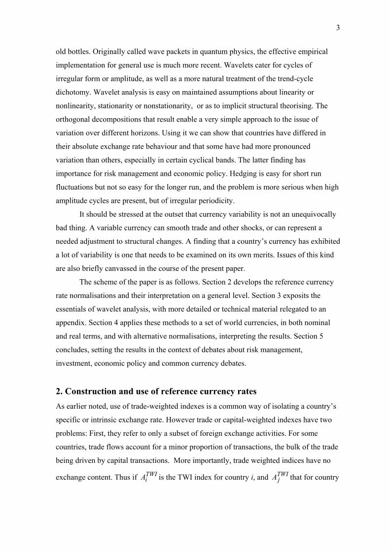
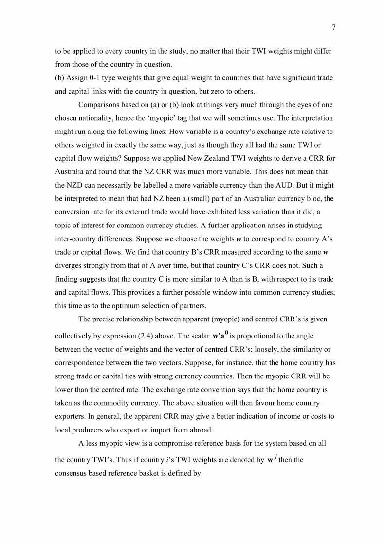
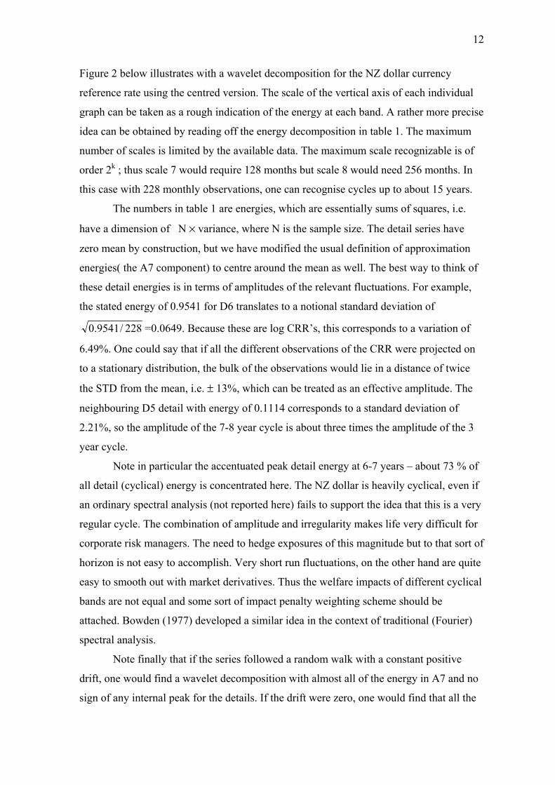
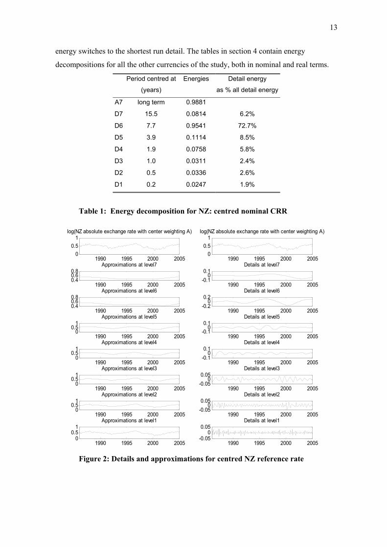
Figure 2 below illustrates with a wavelet decomposition for the NZ dollar currency

reference rate using the centred version. The scale of the vertical axis of each individual

graph can be taken as a rough indication of the energy at each band. A rather more precise

idea can be obtained by reading off the energy decomposition in table 1. The maximum

number of scales is limited by the available data. The maximum scale recognizable is of

order 2k ; thus scale 7 would require 128 months but scale 8 would need 256 months. In

this case with 228 monthly observations, one can recognise cycles up to about 15 years.

The numbers in table 1 are energies, which are essentially sums of squares, i.e.

have a dimension of N × variance, where N is the sample size. The detail series have

zero mean by construction, but we have modified the usual definition of approximation

energies( the A7 component) to centre around the mean as well. The best way to think of

these detail energies is in terms of amplitudes of the relevant fluctuations. For example,

the stated energy of 0.9541 for D6 translates to a notional standard deviation of

228/9541.0 =0.0649. Because these are log CRR’s, this corresponds to a variation of

6.49%. One could say that if all the different observations of the CRR were projected on

to a stationary distribution, the bulk of the observations would lie in a distance of twice

the STD from the mean, i.e. ± 13%, which can be treated as an effective amplitude. The

neighbouring D5 detail with energy of 0.1114 corresponds to a standard deviation of

2.21%, so the amplitude of the 7-8 year cycle is about three times the amplitude of the 3

year cycle.

Note in particular the accentuated peak detail energy at 6-7 years – about 73 % of

all detail (cyclical) energy is concentrated here. The NZ dollar is heavily cyclical, even if

an ordinary spectral analysis (not reported here) fails to support the idea that this is a very

regular cycle. The combination of amplitude and irregularity makes life very difficult for

corporate risk managers. The need to hedge exposures of this magnitude but to that sort of

horizon is not easy to accomplish. Very short run fluctuations, on the other hand are quite

easy to smooth out with market derivatives. Thus the welfare impacts of different cyclical

bands are not equal and some sort of impact penalty weighting scheme should be

attached. Bowden (1977) developed a similar idea in the context of traditional (Fourier)

spectral analysis.

Note finally that if the series followed a random walk with a constant positive

drift, one would find a wavelet decomposition with almost all of the energy in A7 and no

sign of any internal peak for the details. If the drift were zero, one would find that all the

13

energy switches to the shortest run detail. The tables in section 4 contain energy

decompositions for all the other currencies of the study, both in nominal and real terms.

Period centred at

(years)

Energies

Detail energy

as % all detail energy

A7 long term 0.9881

D7 15.5 0.0814 6.2%

D6 7.7 0.9541 72.7%

D5 3.9 0.1114 8.5%

D4 1.9 0.0758 5.8%

D3 1.0 0.0311 2.4%

D2 0.5 0.0336 2.6%

D1 0.2 0.0247 1.9%

Table 1: Energy decomposition for NZ: centred nominal CRR

1990 1995 2000 20050

0.51

log(NZ absolute exchange rate with center weighting A)

1990 1995 2000 20050

0.51

log(NZ absolute exchange rate with center weighting A)

1990 1995 2000 20050.40.60.8

Approximations at level7

1990 1995 2000 2005-0.1

00.1

Details at level7

1990 1995 2000 20050.40.60.8


1990 1995 2000 2005-0.2

00.2

Details at level6

1990 1995 2000 20050

0.51


1990 1995 2000 2005-0.1

00.1

Details at level5

1990 1995 2000 20050

0.51


1990 1995 2000 2005-0.1

00.1

Details at level4

1990 1995 2000 20050

0.51


1990 1995 2000 2005-0.05

00.05

Details at level3

1990 1995 2000 20050

0.51


1990 1995 2000 2005-0.05

00.05

Details at level2

1990 1995 2000 20050

0.51


1990 1995 2000 2005-0.05

00.05

Details at level1

Figure 2: Details and approximations for centred NZ reference rate

14

4. Comparative results The choice of currencies for the present study was influenced by the following

considerations:

(a) A reasonably free exchange rate between 1986 and 2006. Many central banks do

try to smooth their currencies in some way. Japan is an example of a fairly tightly

managed float, while New Zealand was perhaps the world’s most free float, at

least up to 2005. Smoothing was allowed provided the motive was judged to be

stabilisation and not currency fixing.

(b) Absence of any major structural shift that might have affected the currency,

especially conversion during the sample period from fixed to floating. The one

exception to this was Germany. IT was desirable to include a post 1999 Euro zone

currency, and the largest European economy was chosen, notwithstanding a

potential impact from German reunification in the earlier part of the period.

(c) A reasonable geographical coverage. Chile is included as the most structurally

stable South American currency, in spite of doubts3 about whether the Chilean

peso is a truly floating currency, while South Africa also makes the list. We

limited Scandinavia to just Sweden and Norway, the latter being an oil currency

and therefore different.

Calculations cover the following, based on monthly data from 02.1986 to 11.2005.

Exchange rates in all cases are logs as in section II. References are to the full tables,

which appear in Appendix C.

1. Centred log exchange rates for nominal (Table C1) and real exchange rates (Table C2).

The reference basket is an equally weighted in all included currencies.

2. Apparent exchange rates. We chose New Zealand as the home country, influenced also

by recent debates about monetary policy and common currencies. Two versions of the

reference basket w were chosen as in table 2. Weights A are simple (0-1 style) selection

weights based on both the trade weights and what is known about major capital flows,

such as international borrowing and its ultimate sources4. Weights B are the TWI weights

as of 2005, except that the weights for the Euro zone are transferred in their entirety to

Germany.

15

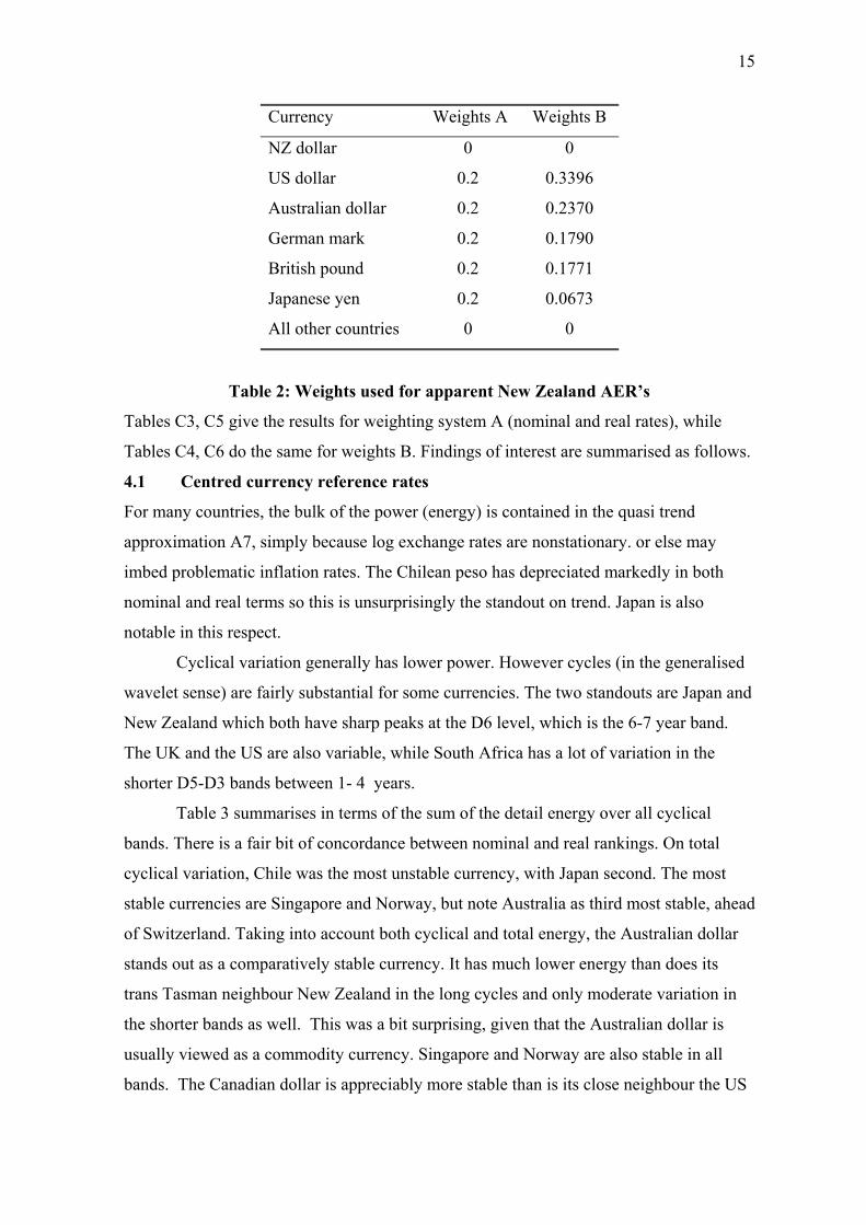
Currency Weights A Weights B

NZ dollar 0 0

US dollar 0.2 0.3396

Australian dollar 0.2 0.2370

German mark 0.2 0.1790

British pound 0.2 0.1771

Japanese yen 0.2 0.0673

All other countries 0 0

Table 2: Weights used for apparent New Zealand AER’s

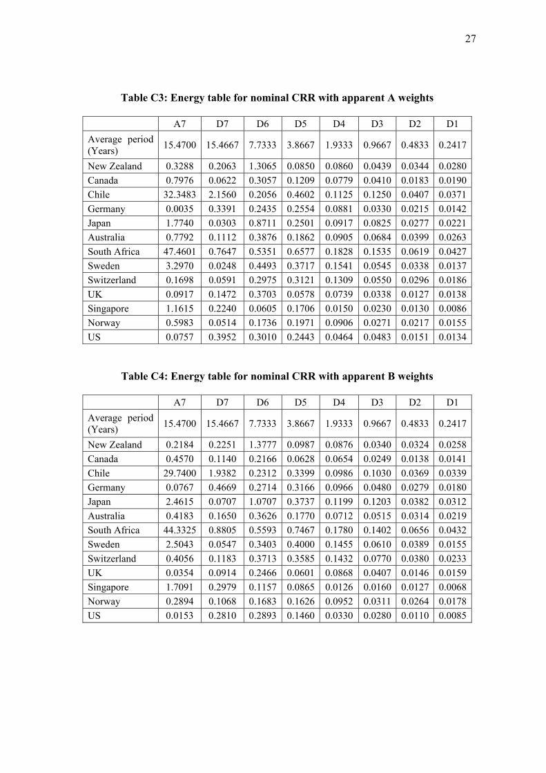
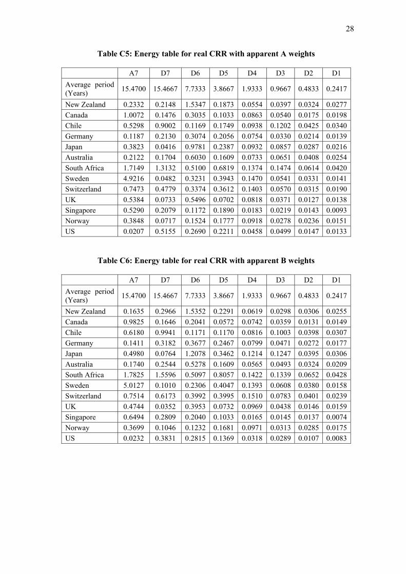
Tables C3, C5 give the results for weighting system A (nominal and real rates), while

Tables C4, C6 do the same for weights B. Findings of interest are summarised as follows.

4.1 Centred currency reference rates

For many countries, the bulk of the power (energy) is contained in the quasi trend

approximation A7, simply because log exchange rates are nonstationary. or else may

imbed problematic inflation rates. The Chilean peso has depreciated markedly in both

nominal and real terms so this is unsurprisingly the standout on trend. Japan is also

notable in this respect.

Cyclical variation generally has lower power. However cycles (in the generalised

wavelet sense) are fairly substantial for some currencies. The two standouts are Japan and

New Zealand which both have sharp peaks at the D6 level, which is the 6-7 year band.

The UK and the US are also variable, while South Africa has a lot of variation in the

shorter D5-D3 bands between 1- 4 years.

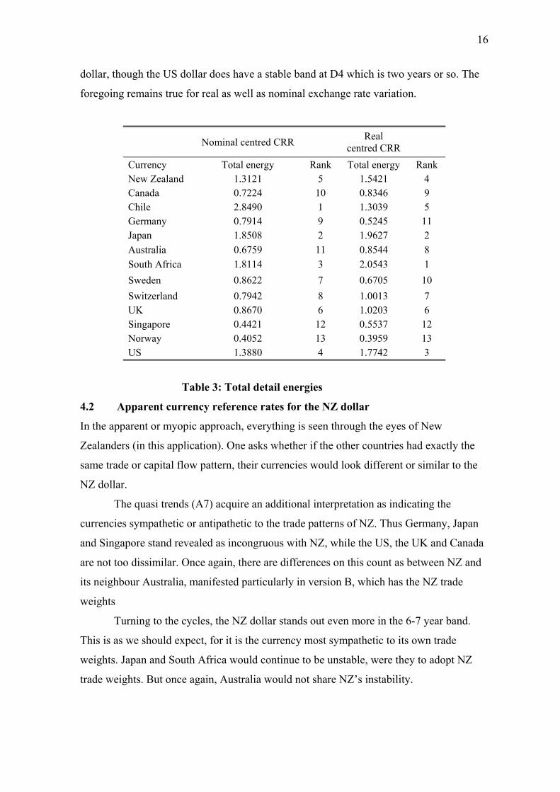
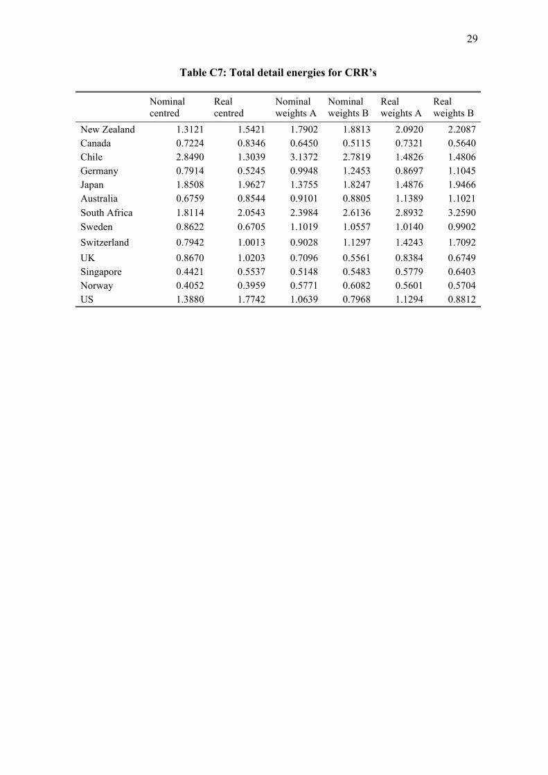
Table 3 summarises in terms of the sum of the detail energy over all cyclical

bands. There is a fair bit of concordance between nominal and real rankings. On total

cyclical variation, Chile was the most unstable currency, with Japan second. The most

stable currencies are Singapore and Norway, but note Australia as third most stable, ahead

of Switzerland. Taking into account both cyclical and total energy, the Australian dollar

stands out as a comparatively stable currency. It has much lower energy than does its

trans Tasman neighbour New Zealand in the long cycles and only moderate variation in

the shorter bands as well. This was a bit surprising, given that the Australian dollar is

usually viewed as a commodity currency. Singapore and Norway are also stable in all

bands. The Canadian dollar is appreciably more stable than is its close neighbour the US

16

dollar, though the US dollar does have a stable band at D4 which is two years or so. The

foregoing remains true for real as well as nominal exchange rate variation.

Nominal centred CRR Real centred CRR

Currency Total energy Rank Total energy Rank New Zealand 1.3121 5 1.5421 4 Canada 0.7224 10 0.8346 9 Chile 2.8490 1 1.3039 5 Germany 0.7914 9 0.5245 11 Japan 1.8508 2 1.9627 2 Australia 0.6759 11 0.8544 8 South Africa 1.8114 3 2.0543 1 Sweden 0.8622 7 0.6705 10 Switzerland 0.7942 8 1.0013 7 UK 0.8670 6 1.0203 6 Singapore 0.4421 12 0.5537 12 Norway 0.4052 13 0.3959 13 US 1.3880 4 1.7742 3

Table 3: Total detail energies

4.2 Apparent currency reference rates for the NZ dollar

In the apparent or myopic approach, everything is seen through the eyes of New

Zealanders (in this application). One asks whether if the other countries had exactly the

same trade or capital flow pattern, their currencies would look different or similar to the

NZ dollar.

The quasi trends (A7) acquire an additional interpretation as indicating the

currencies sympathetic or antipathetic to the trade patterns of NZ. Thus Germany, Japan

and Singapore stand revealed as incongruous with NZ, while the US, the UK and Canada

are not too dissimilar. Once again, there are differences on this count as between NZ and

its neighbour Australia, manifested particularly in version B, which has the NZ trade

weights

Turning to the cycles, the NZ dollar stands out even more in the 6-7 year band.

This is as we should expect, for it is the currency most sympathetic to its own trade

weights. Japan and South Africa would continue to be unstable, were they to adopt NZ

trade weights. But once again, Australia would not share NZ’s instability.

17

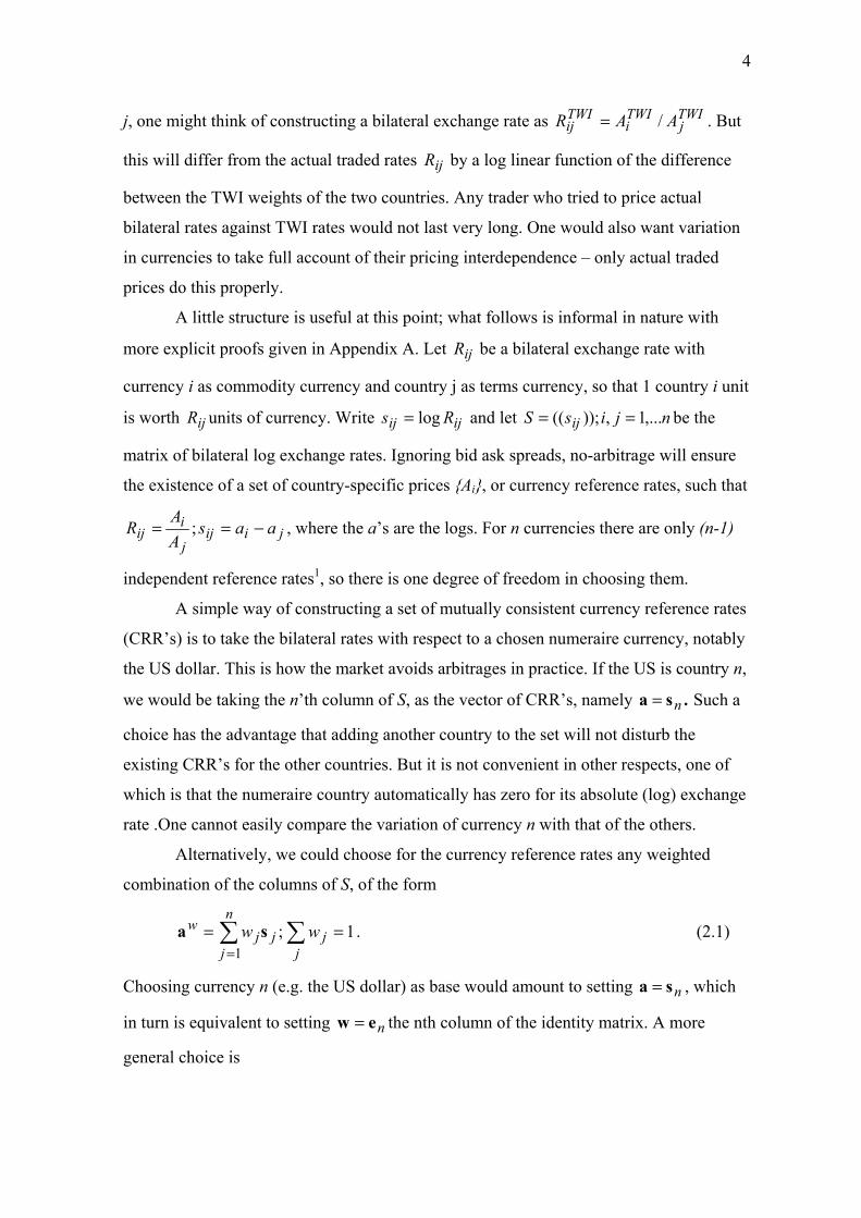
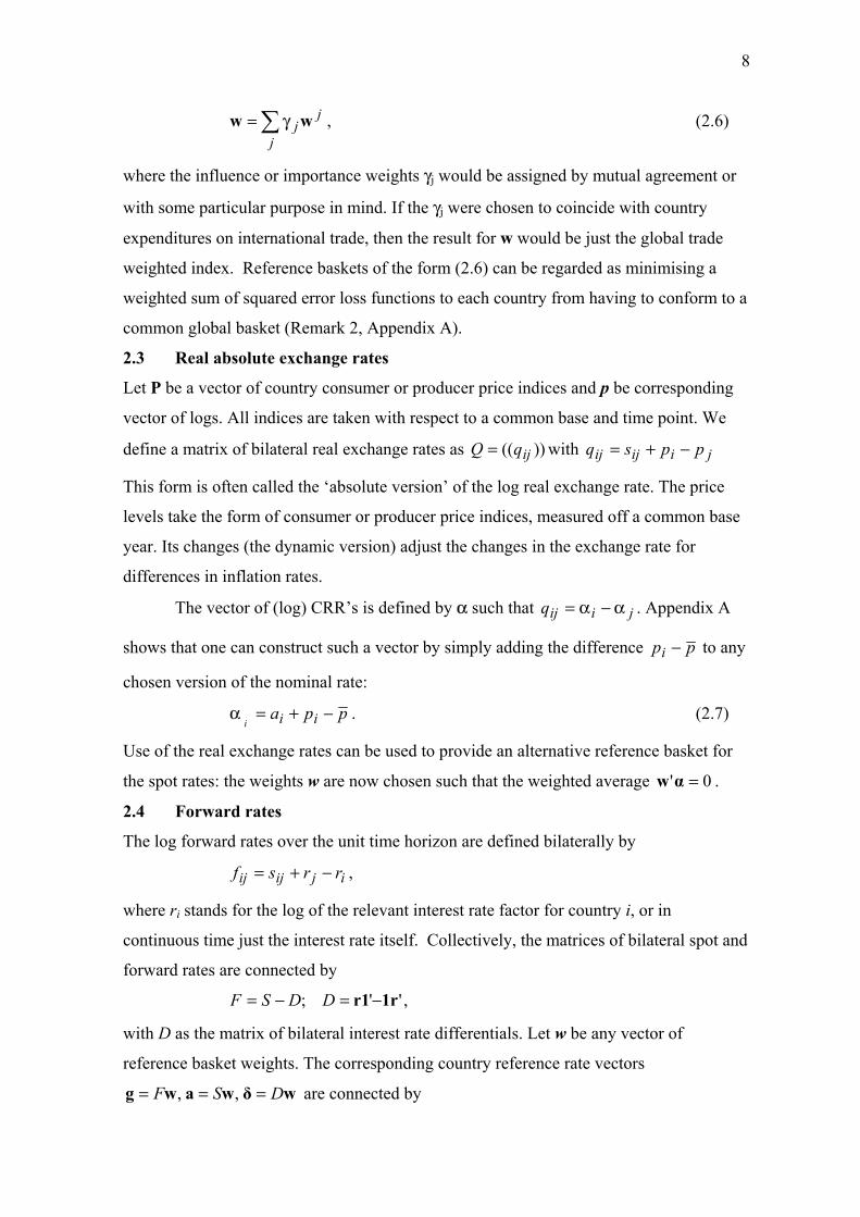
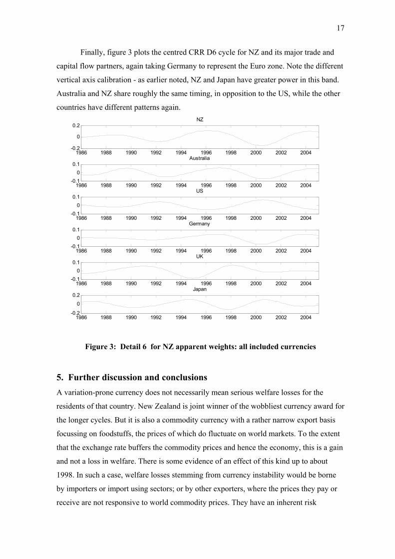
Finally, figure 3 plots the centred CRR D6 cycle for NZ and its major trade and

capital flow partners, again taking Germany to represent the Euro zone. Note the different

vertical axis calibration - as earlier noted, NZ and Japan have greater power in this band.

Australia and NZ share roughly the same timing, in opposition to the US, while the other

countries have different patterns again.

1986 1988 1990 1992 1994 1996 1998 2000 2002 2004-0.2

0

0.2NZ

1986 1988 1990 1992 1994 1996 1998 2000 2002 2004-0.1

00.1

Australia

1986 1988 1990 1992 1994 1996 1998 2000 2002 2004-0.1

00.1

US

1986 1988 1990 1992 1994 1996 1998 2000 2002 2004-0.1

00.1

Germany

1986 1988 1990 1992 1994 1996 1998 2000 2002 2004-0.1

00.1

UK

1986 1988 1990 1992 1994 1996 1998 2000 2002 2004-0.2

0

0.2Japan

Figure 3: Detail 6 for NZ apparent weights: all included currencies

5. Further discussion and conclusions A variation-prone currency does not necessarily mean serious welfare losses for the

residents of that country. New Zealand is joint winner of the wobbliest currency award for

the longer cycles. But it is also a commodity currency with a rather narrow export basis

focussing on foodstuffs, the prices of which do fluctuate on world markets. To the extent

that the exchange rate buffers the commodity prices and hence the economy, this is a gain

and not a loss in welfare. There is some evidence of an effect of this kind up to about

1998. In such a case, welfare losses stemming from currency instability would be borne

by importers or import using sectors; or by other exporters, where the prices they pay or

receive are not responsive to world commodity prices. They have an inherent risk

18

management problem with some tough decisions as to either or not to hedge the currency

exposure. Hedging is not too difficult an exercise if the problem is very short run

fluctuation, over a matter of months rather than years. Simple smoothing devices based on

staggered forwards will suffice for this. It becomes much more difficult, with issues of

passive versus active timing, if the exposures are to longer cycles, or uncertain

periodicity. The existence of a forward discount on the home currency will not help its

exporters if they lock into a forward rate and the home currency then devalues well

beyond that level. The timing of long term forwards is not a trivial matter and it becomes

more difficult if cycles are known to exist but they are irregular as to periods. In addition,

long term forwards are available only to extremely good credit risks, and many exporters

would not qualify, especially start up ventures. The potential risk exposure is higher the

wider the amplitudes of the cycles, or in wavelet terms, the greater the energy.

Moreover, even the buffering effect on major commodity exporters is now in

doubt. Bowden and Zhu (2006a) point out that post 1998, the effect has been inoperative,

as the NZ economy has become increasingly exposed to flows of offshore capital. The

energies may be getting larger and the problem of risk management more pressing, for all

exporters and importers. It does seem to be the case that the narrower the export base, the

more variable the currency. Like New Zealand, Australia tends to be regarded as a

commodity currency, but this extends to oil and gas, metals and other commodity

classifications which NZ does not have, and which have their own industrial usage and

price cycles. But one should also note the independent influence of capital flows,

particularly with the US, the UK and Japan, all of which are quite variable in their

currencies yet have a well diversified export base.

An unstable currency could also be accentuated by monetary policies aimed at

inflation control. A case could be made that in recent years the swings in the NZ dollar

have been exacerbated by the central bank’s inflation targeting regime or the way that it is

run. In particular, the practice of signalling future cash rate rises has been seen as giving

comfort to hedge funds and the carry trade, whereby they fund in the USD or Japanese

yen and invest in NZ dollar rates. If the currency effects of their actions neutralises the

commodity price buffering effect, then that is a general welfare loss to New Zealanders.

Variable currencies and their typical periodicity will also preoccupy investors and

fund managers. The return on any offshore investment is the sum of its local return (or

intrinsic own-currency return) and the currency return when translated back to the

investor’s home currency. The received doctrine is that foreign diversification is a good

19

thing. But if currencies can exhibit pronounced cyclical variability in the currency

component, uncompensated by the intrinsic return, then investors acquire an exposure to a

form of timing risk. Specifically, they incur negative currency returns if their entry or exit

are, for one reason or another, not well timed. This effect is more serious with the longer

cycles, for the investor may not be in a position to wait for 3 or 4 years for things to

improve. Bowden and Zhu (2006b) have drawn attention to this problem, proposing exit

risk as one criterion for portfolio selection.

As in most forms of economic life, to become aware of a thing is to change it. If

fund managers do become aware of substantial currency cycles, then they will tend to

invest at the low point and divest at the high point. This, together with the ever increasing

globalisation of capital markets, might mean that movements in the currency become

more violent at or near peaks or troughs. There is indeed some recent evidence of this in

the round of currency realignments now going on.

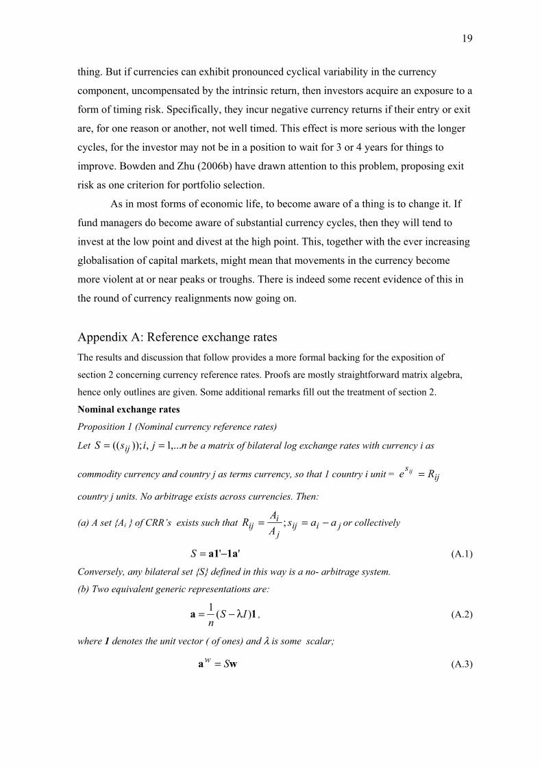
Appendix A: Reference exchange rates The results and discussion that follow provides a more formal backing for the exposition of

section 2 concerning currency reference rates. Proofs are mostly straightforward matrix algebra,

hence only outlines are given. Some additional remarks fill out the treatment of section 2.

Nominal exchange rates

Proposition 1 (Nominal currency reference rates)

Let njisS ij ,...1,));(( == be a matrix of bilateral log exchange rates with currency i as

commodity currency and country j as terms currency, so that 1 country i unit = ijs Re ij =

country j units. No arbitrage exists across currencies. Then:

(a) A set Ai of CRR’s exists such that jiijj

iij aas

AA

R −== ; or collectively

'' 1aa1 −=S (A.1)

Conversely, any bilateral set S defined in this way is a no- arbitrage system.

(b) Two equivalent generic representations are:

1a )(1 ISn

λ−= , (A.2)

where 1 denotes the unit vector ( of ones) and λ is some scalar;

wa Sw = (A.3)

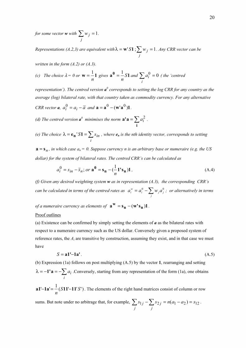
20

for some vector w with 1=∑j

jw .

Representations (A.2,3) are equivalent with ∑ ==λj

jwS 1;' 1w . Any CRR vector can be

written in the form (A.2) or (A.3).

(c) The choice λ = 0 or 1wn1= gives 1a0 S

n1= and ∑ =

iia 00 ( the ‘centred

representation’). The centred version a0 corresponds to setting the log CRR for any country as the

average (log) bilateral rate, with that country taken as commodity currency. For any alternative

CRR vector a, aaa ii −=0 and 1awaa )'( 00 −= .

(d) The centred version a0 minimises the norm ∑=i

aa' 2ia .

(e) The choice ∑==λi

insS1en ' , where en is the nth identity vector, corresponds to setting

nsa = , in which case an = 0. Suppose currency n is an arbitrary base or numeraire (e.g. the US

dollar) for the system of bilateral rates. The centred CRR’s can be calculated as

1s1'sa nn0 )1(;0

norssa nini −=−= , (A.4)

(f) Given any desired weighting system w as in representation (A.3), the corresponding CRR’s

can be calculated in terms of the centred rates as ∑−=j

jjiwi awaa 00 ; or alternatively in terms

of a numeraire currency as elements of 1sw'sa nnw )(−= .

Proof outlines

(a) Existence can be confirmed by simply setting the elements of a as the bilateral rates with

respect to a numeraire currency such as the US dollar. Conversely given a proposed system of

reference rates, the Ai are transitive by construction, assuming they exist, and in that case we must

have

1a'a1'−=S . (A.5)

(b) Expression (1a) follows on post multiplying (A.5) by the vector 1, rearranging and setting

∑−=−=λi

iaa1' .Conversely, starting from any representation of the form (1a), one obtains

)'''(1'' SSn

11111aa1 −=− . The elements of the right hand matrices consist of column or row

sums. But note under no arbitrage that, for example, 122121 )( saanssj

jj

j =−=−∑∑ .

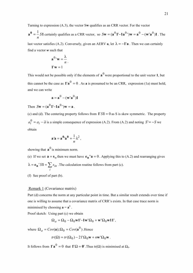
21

Turning to expression (A.3), the vector Sw qualifies as an CRR vector. For the vector

1a0 Sn1= certainly qualifies as a CRR vector, so 1awaw1a1aw )'()''( 0000 −=−=S . The

last vector satisfies (A.2). Conversely, given an AERV a, let a1'−=λ . Then we can certainly

find a vector w such that

1'

'0

=

λ=

w1

wan .

This would not be possible only if the elements of 0a were proportional to the unit vector 1, but

this cannot be the case as 0' 0 =a1 . As a is presumed to be an CRR, expression (1a) must hold,

and we can write

1awaa )'( 00 −=

Then aw1a1aw =−= )''( 00S .

(c) and (d). The centering property follows from 0' =11 S as S is skew symmetric. The property

aaa ii −=0 is a simple consequence of expression (A.2). From (A.2) and noting SS −=' we

obtain

21 λ+=n

'' 00 aaaa ,

showing that 0a is minimum norm.

(e) If we set nsa = then we must have 0=a'en . Applying this to (A.2) and rearranging gives

∑==λi

insS1en ' .The calculation routine follows from part (c).

(f) See proof of part (b).

Remark 1 (Covariance matrix)

Part (d) concerns the norm at any particular point in time. But a similar result extends over time if

one is willing to assume that a covariance matrix of CRR’s exists. In that case trace norm is

minimised by choosing a = a0 .

Proof sketch: Using part (c) we obtain

'''' 0000 w11w1ww1 Ω+Ω−Ω−Ω=Ωa ,

where )();( 00 aa CovCova =Ω=Ω .Hence

www 000 ''21)()( Ω+Ω−Ω=Ω ntrtr .

It follows from 0' 0 =a1 that '' 01 =Ω .Thus tr(Ω) is minimised at Ω0.

22

Remark 2 ( Consensus-based reference baskets)

As noted in section II, a general approach might be to seek a compromise between country TWI’s

or capital weighted indexes, while preserving the exchange feature. Thus let jjS aw = be the

CRR that might be chosen by country j to conform to its own TWI weight pattern jw . As noted

earlier, this would have the property that 0=jj a'w , so if the international agreement was for a

compromise weighting giving an AER vector wa S= , the loss to country j might be of the order

of jwa' . Considering all countries together, we could imagine them settling on a global

weighting defined by 1';'minarg2

==γ= ∑ w1andwawaw w Sj

jj

g .

In this expression, semipositive weights γj ; ∑ =γj

j 1are used to indicate degrees of importance

or ‘economic clout’ of the economy concerned. The optimum is given by

1aa λ−= 0 where ∑ =λλγ=λj

jjjj

0'; aw .

Equivalently, just set the weights w as the weighted average of the individual country weights

jw .

∑ γ=j

jjww .

B: Real exchange rates

Collectively, the matrix of bilateral real rates is defined by

'' 1pp1 −+= SQ . (A.6)

Sought is a vector α of real currency reference rates such that

'' 1αα1 −=Q (A.7)

Proposition 2 (Real currency reference rates)

(a) The absolute real exchange rates are generated by the form

α11α ';)(1 −=λλ−= α IQn

. (A.8)

(b) The choice λα = 0 yields the zero centred real exchange rate α0 , and this is can be obtained in

terms of the zero centred nominal exchange rate a0 as

∑=−+=i

ipn

p;p 100 1paα . (A.9)

(c) More generally, given any nominal exchange rate centering (value of λ), one can

generate a corresponding real exchange rate as

23

)( 1paα p−+= λ

with λ=λα .

Proof outlines

(a) As for part (a) of Proposition 1.

(b) Follows from the skew symmetry of Q, while expression (A.9) is obtained by expressing Q in

terms of S using expression (A.6).

(c) Combine expressions A.6-A.8.

Remark 3

Proposition 2 gives us yet another economically meaningful value of λ for the nominal rate,

namely ∑==λi

inqQ1en ' , which corresponds to setting the numeraire of the system as

country n’s real exchange rate.

Appendix B: Wavelet analysis Wavelet analysis has been slow in its uptake into general empirical economics. What

follows is a brief account of features of wavelet analysis as they apply to the present

study.

Wavelet decompositions

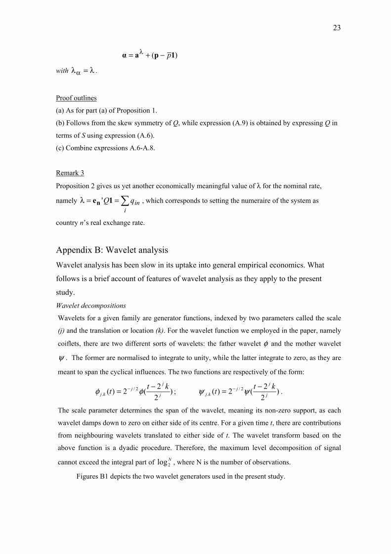
Wavelets for a given family are generator functions, indexed by two parameters called the scale

(j) and the translation or location (k). For the wavelet function we employed in the paper, namely

coiflets, there are two different sorts of wavelets: the father wavelet φ and the mother wavelet

ψ . The former are normalised to integrate to unity, while the latter integrate to zero, as they are

meant to span the cyclical influences. The two functions are respectively of the form:

)22(2)( 2/

. j

jj

kjktt −= − φφ ; )

22(2)( 2/

. j

jj

kjktt −= − ψψ .

The scale parameter determines the span of the wavelet, meaning its non-zero support, as each

wavelet damps down to zero on either side of its centre. For a given time t, there are contributions

from neighbouring wavelets translated to either side of t. The wavelet transform based on the

above function is a dyadic procedure. Therefore, the maximum level decomposition of signal

cannot exceed the integral part of N2log , where N is the number of observations.

Figures B1 depicts the two wavelet generators used in the present study.

24

Figure B1: Coiflet father wavelet (left) and mother wavelet (right)

The family of functions defined as above are mutually orthogonal. In a manner analogous

to Fourier analysis one can form coefficients as

dtttxs kJkJ ∫ φ= )()( ,, ; dtttxd kjkj ∫ ψ= )()( ,, ,

for j = 1,2…J , where J is limited by the number of observations available on the given series

x(t), supposed continuous here for simplicity. As with the inverse transform in Fourier analysis,

we can recover x(t) in terms the wavelet functions as:

∑∑∑∑ ψ++ψ+ψ+φ= −−k

kkk

kJkJk

kJkJk

kJkJ tdtdtdtstx )(...)()()()( ,1,1,1,1,,,, .

We write ∑ ψ=k

kjkjj tdtD )()( ,, . Note that just the one father wavelet has been used in the

above, with maximal scale.

Computational procedure

The quasi Fourier approach illustrated above would be slow computationally. In the present

paper, computations were done in Matlab (Misiti et al 2005) using Mallat’s algorithm, which is

considerably more efficient. The algorithm follows through the basic sequence as illustrated in

figure 2 of the text. The original signal x(t) is fed through a high pass and low pass filter, one the

quadrature of the other, which ensures orthogonality of the two outputs. The low pass filter is

adapted to the longer run father wavelets and the higher to the mother wavelets. Output from the

high pass filter is downloaded as the level 1 detail D1, and the output from the low pass filter

becomes the level 1 Approximation. Starting afresh with A1, the process is successively repeated.

Wavelet variances and covariances

By decomposing the time series into orthogonal components as above, the variance of

components at different scales can be derived. The DWT provides a simple way of computing

these that closely parallels the classical statistical formulas. For each detail level j, the average

energy or power over the horizon can be expressed as the percentage contribution of each level of

detail relative to the whole as:

25

∑∑∑

∑∑

+=

==

j ttj

ttj

ttj

Aj

ttj

Dj

DAE

AE

EDE

E

2,

2,

2,

2,

1,1

The DWT variance computations can be improved using the maximal-overlap discrete wavelet

transform (MODWT) estimator of the wavelet variance (Percival 1995). We have chosen not to

use this as it assumes circularity, in other words the historical series simply repeats itself.

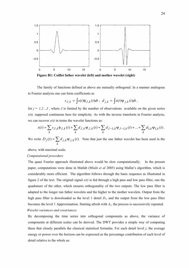
Scale and frequency

To connect the scale to frequency, a pseudo frequency is calculated. The algorithm works by

associating with the wavelet function a purely periodic signal of frequency Fc that maximizes the

Fourier transform of the wavelet modulus. When the wavelet is dilated by the scaling factor 2j,

the pseudo frequency corresponding to the scale is expressed as:

,2 ∆×

= jc

sF

F

where ∆ is the sampling interval.

Taking the wavelet ‘coif5’ as an example, the centre frequency (figure B2) is 0.68966 and thus

the pseudo frequency corresponding to the scale 25 is 0.02155. As the sampling period is one

month, the period corresponding to the pseudo frequency is 3.87 years.

Figure B2: Scale in terms of equivalent sinusoidal frequency

0 5 10 15 20 25 30 - 1

- 0.5

0

0.5

1

1.5 Wavelet coif5 and center frequency based approximation

Period: 1.45; Cent. Freq: 0.68966

26

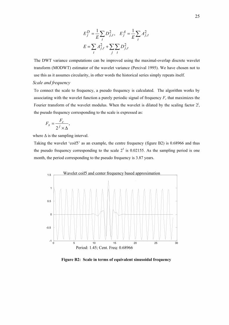
Appendix C: Detailed result tables The tables that follow give energy decompositions for different versions of the reference currency

rates. Note that these are quasi variances for orthogonal details, so to get total energy, just sum

across the columns or a selection of columns.

Table C1: Energy table for nominal CRR, centred version

A7 D7 D6 D5 D4 D3 D2 D1

Average period (Years) 15.4700 15.4667 7.7333 3.8667 1.9333 0.9667 0.4833 0.2417

New Zealand 0.9881 0.0814 0.9541 0.1114 0.0758 0.0311 0.0336 0.0247Canada 0.3188 0.1101 0.3893 0.0891 0.0708 0.0310 0.0168 0.0153Chile 20.7024 1.9569 0.2270 0.3753 0.1192 0.1004 0.0378 0.0324Germany 1.3631 0.2958 0.1070 0.2250 0.0925 0.0385 0.0183 0.0143Japan 6.0133 0.0614 1.1145 0.3927 0.1138 0.1122 0.0300 0.0262Australia 0.1236 0.0414 0.2212 0.1972 0.0866 0.0590 0.0427 0.0278South Africa 33.1305 0.5170 0.3484 0.5746 0.1555 0.1276 0.0525 0.0358Sweden 0.4610 0.0645 0.3215 0.2526 0.1358 0.0487 0.0280 0.0111Switzerland 2.3703 0.0790 0.1925 0.2842 0.1298 0.0639 0.0256 0.0192UK 0.9174 0.2612 0.3955 0.0627 0.0769 0.0363 0.0173 0.0171Singapore 4.6753 0.1226 0.1457 0.1228 0.0113 0.0210 0.0115 0.0072Norway 0.1925 0.0789 0.0668 0.1299 0.0766 0.0242 0.0154 0.0134US 0.7852 0.5128 0.5267 0.2372 0.0416 0.0409 0.0176 0.0112

Table C2: Energy table for real CRR, centred version

A7 D7 D6 D5 D4 D3 D2 D1 Average period (Years) 15.4700 15.4667 7.7333 3.8667 1.9333 0.9667 0.4833 0.2417


27

Table C3: Energy table for nominal CRR with apparent A weights



Table C4: Energy table for nominal CRR with apparent B weights



28

Table C5: Energy table for real CRR with apparent A weights



Table C6: Energy table for real CRR with apparent B weights



29

Table C7: Total detail energies for CRR’s

Nominal centred

Real centred

Nominal weights A

Nominal weights B

Real weights A

Real weights B

New Zealand 1.3121 1.5421 1.7902 1.8813 2.0920 2.2087Canada 0.7224 0.8346 0.6450 0.5115 0.7321 0.5640Chile 2.8490 1.3039 3.1372 2.7819 1.4826 1.4806Germany 0.7914 0.5245 0.9948 1.2453 0.8697 1.1045Japan 1.8508 1.9627 1.3755 1.8247 1.4876 1.9466Australia 0.6759 0.8544 0.9101 0.8805 1.1389 1.1021South Africa 1.8114 2.0543 2.3984 2.6136 2.8932 3.2590Sweden 0.8622 0.6705 1.1019 1.0557 1.0140 0.9902Switzerland 0.7942 1.0013 0.9028 1.1297 1.4243 1.7092UK 0.8670 1.0203 0.7096 0.5561 0.8384 0.6749Singapore 0.4421 0.5537 0.5148 0.5483 0.5779 0.6403Norway 0.4052 0.3959 0.5771 0.6082 0.5601 0.5704US 1.3880 1.7742 1.0639 0.7968 1.1294 0.8812

30

References

Bowden, R. J. and J. Zhu (2006a): “The agribusiness cycles and its wavelets,” working paper, School of Economics and Finance, Victoria University of Wellington, New Zealand.

Bowden, R. J. and J. Zhu (2006b): “Beyond the short run: The longer time scale

volatility of investment value,” working paper, School of Economics and Finance, Victoria University of Wellington, New Zealand.

Bowden, R. J. and J. Zhu (2005): Kiwicap: An introduction to New Zealand Capital Markets,

Wellington: Kiwicap Education. Bowden, R. J. (1977): “Spectral utility functions and the design of a stationary system,”

Econometrica, vol 45, no 4, 1007-1012. Cohen, A., Daubechies, I., and Feauveau, J.C. (1992): “Biorthogonal basis of compactly

supported wavelets,” Communications in Pure and Applied Mathematics, vol. 45, 485-560.

Coifman, R., Meyer, Y., Quake, S. and Wickerhauser, V. (1990): “Signal processing and

compression with wavelet packets,” Numerical Algorithms Research Group, Yale University, New Haven, CT, USA.

Crowley, P. (2005): “An intuitive guide to wavelets,” Bank of Finland/College of Business

Texas A&M University, [email protected] Daubechies, I. (1988): “Orthonormal bases of compactly supported wavelets,”

Communications on Pure and Applied Mathematics 41: 909-96. Daubechies, I. (1990): “The wavelet transform, time-frequency localization and signal

analysis,” IEEE Transactions on Information Theory, vol. 36, no. 5, 961-1005. Daubechies, I. (1992): “Ten lectures on wavelets,” Society for Industrial and Applied

Mathematics, Capital City Press, Montpelier, VT, USA. Engel, C. and J. Hamilton (1990): “Long Swings in the Dollar: Are They in the Data and Do

Markets Know It?” American Economic Review, 80, 689-713. Guo, H., and R. Savickas (2005): “Foreign Exchange Rates Don’t Follow a Random Walk,”

working paper, Federal Reserve Bank of St. Louis. Hodrick, R. J. (1987): The Empirical Evidence of the Efficiency of Forward and Futures

Foreign Exchange Markets, New York: Harwood Academic. Kaminsky, G. (1993): “Is there a peso problem? Evidence from the dollar/pound exchange

rate, 1976-1987,” American Economic Review, 83, 450-472. Levich, R. M. (2001): International Financial Markets, 2nd ed., NewYork: McGraw-Hill.

31

Mallat, S. (1989): “A theory for multiresolution signal decomposition: the wavelet representation,” IEEE Transactions on Pattern Analysis and Machine Intelligence 11: 674-93.

Misiti, Michel, Yves Misiti, Georges Oppenheim and Jean-Michel Poggi (2005): Wavelet

Toolbox user’s guide, www.mathworks.comn. Percival, D. P. (1995): “On estimation of the wavelet variance”, Biometrika 82, 619-623. Ramsey, J. (1999): “The contribution of wavelets to the analysis of economic and financial

data,” Phil. Trans. R. Soc. Lond. A 357, 2593-2606 Schleicher, C. (2002): “An introduction to wavelets for economists,” Bank of Canada

Working Paper 2002-3.

32

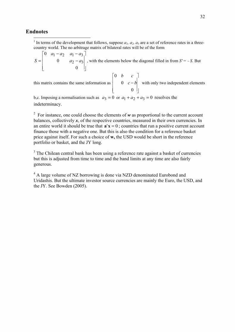
Endnotes 1 In terms of the development that follows, suppose a1, a2, a3 are a set of reference rates in a three- country world. The no arbitrage matrix of bilateral rates will be of the form

⎥⎥⎥

⎦

⎤

⎢⎢⎢

⎣

⎡−−−

=0

00

32

3121aaaaaa

S , with the elements below the diagonal filled in from S' = - S. But

this matrix contains the same information as ⎥⎥⎥

⎦

⎤

⎢⎢⎢

⎣

⎡−0

00

bccb

with only two independent elements

b,c. Imposing a normalisation such as 03 =a or 0321 =++ aaa resolves the indeterminacy. 2 For instance, one could choose the elements of w as proportional to the current account balances, collectively x, of the respective countries, measured in their own currencies. In an entire world it should be true that 0' =xa ; countries that run a positive current account finance those with a negative one. But this is also the condition for a reference basket price against itself. For such a choice of w, the USD would be short in the reference portfolio or basket, and the JY long. 3 The Chilean central bank has been using a reference rate against a basket of currencies but this is adjusted from time to time and the band limits at any time are also fairly generous. 4 A large volume of NZ borrowing is done via NZD denominated Eurobond and Uridashis. But the ultimate investor source currencies are mainly the Euro, the USD, and the JY. See Bowden (2005).

Documents

Which are the world's wobblier currencies? Reference exchange