Embed Size (px)
Citation preview

1
WHICH HUMAN CAPITAL MATTERS FOR RICH AND POOR’S WAGES? EVIDENCE FROM MATCHED WORKER-FIRM DATA FROM TUNISIA *
Christophe Muller and Christophe Nordman **
WP-AD 2004-28
Corresponding autor: C. Muller, Departamento de Fundamentos del Análisis Económico, Universidad de Alicante, Campus de San Vicente, 03080 Alicante, Spain. Email: [email protected] Editor: Instituto Valenciano de Investigaciones Económicas, S.A. Primera Edición Julio 2004. Depósito Legal: V-3363-2004 IVIE working papers offer in advance the results of economic research under way in order to encourage a discussion process before sending them to scientific journals for their final publication.
* This paper has been supported by the ESRC under the grant no. R000230326. The first author is also grateful for the financial support by Spanish Ministry of Sciences and Technology, Project No. BEC2002-0309, and by the Instituto Valenciano de Investigaciones Economicas. We gratefully acknowledge comments from participants in a seminar in DIAL in Paris, in the Third Euro-Mediterraneen Days in Ifrane, in the Conference on Labour Market Models and Matched Employer-Employee Data in Sonderborg. Usual disclaimers apply. ** Institut de Recherche pour le Développement - DIAL (Développement et Insertion Internationale), 4 rue d'Enghein 75010, Paris. Emails: [email protected] ; [email protected]
2
WHICH HUMAN CAPITAL MATTERS FOR RICH AND POOR’S WAGES?
EVIDENCE FROM MATCHED WORKER-FIRM DATA FROM TUNISIA
Christophe Muller and Christophe Nordman
ABSTRACT
In this paper, we study the return to human capital variables for wages of workers observed in Tunisian matched worker-firm data in 1999. We develop a new method based on multivariate analysis of firm characteristics, which allows us most of the benefits obtained by introducing firm dummies in wage equations. It also provides a human capital interpretation of the effect of these dummy variables. Moreover, in the studied data, using three firm characteristics easily collectable yields results close to those obtained by using the matched structure of the data.
The poorest workers (as defined in terms of wage levels or by conditional wages in quantile regressions) experience greater returns to human capital than workers belonging to the middle of the wage distribution. However, the return to schooling of the poorest workers is significantly lower than that of the richest workers. Wage regressions including the computed factors confirm that human capital is associated with positive intra-firm externality on wages. Therefore, a given worker would be more productive and better paid in an environment strongly endowed in human capital. However, the poorest workers do not take advantage of the structure of human capital in the firm. Conversely, the poor benefit from working in the textile sector in terms of wages unlike the middle and high wage workers. Finally, the poorest and richest workers benefit from an innovative environment while the middle workers of the wage distribution do not. Keywords: wage, returns to human capital, matched worker-firm data, quantile regressions,
factor analysis, Tunisia JEL Classification: J24, J31, O12

3
1. Introduction
1.1 Worker or firm knowledge?
Returns to human capital and skills have always been considered dominant explanations for labour compensation. Accordingly, they have been incorporated in individual wage equations by using regressors describing schooling and the worker’s experience1. This is particularly important for developing countries where the returns to education are expected to be higher2. A variety of human capital indicators have been used for this purpose, although it is fair to say the number of schooling years and number of work experience years are the most popular regressors in similar wage equations, often accompanied by their squared values.
On the other hand, it has been recognized for a long time that some skills or human capital attributed to workers are also specific to the firm in which she works. The experience accumulated within the firm may be different from experience previously obtained outside the firm. Thus, part of the return to human capital for the worker remuneration can be viewed as if it originated from the firm.
Moreover, the endogenous growth literature emphasizes the presence of technological or social externalities that generate higher returns to traditional factors, notably labour. It is likely that some of these externalities occur in the form of general knowledge that may be diffused in the economy or the considered activity sector. It is also probable that many externalities actually take place in the firm where the worker operates since that is where the technological processes are most frequently exhibited and transmitted.
Thus, the overall return to human capital explaining the remuneration of a given worker may involve personal skill characteristics and firm knowledge characteristics. It seems important to consider these two sources of returns to human capital simultaneously because education policies and policies promoting vocational training may affect the worker’s and the firm’s human capital environment differently. In particular, assessing policies without accounting for educational and knowledge externalities within firms may under-estimate the benefits of such policies.
1 Mincer (1993); Card (1999). 2 Sahn and Alderman (1988), Hoddinott (1996), Behrman (1999).

4
Finally, distinguishing the two sources of human capital may contribute to explain the typical over-estimation of returns to schooling in LDCs, as mentioned in Behrman (1999), which occurs while neglecting intra-firm human capital externalities. Indeed, part of the impact of knowledge on productivities may be caused by these externalities, associated or not with specific firm processes and working rules.
1.2 Crucial data
One popular way to account for firm characteristics, including for their human capital features, is to base the econometric investigation on matched worker-firm data3. Mostly, dummy variables for individual firms are added as independent variables in usual wage equations. We shall avail ourselves of such data, for the first time in the Tunisia case. We focus our investigation on Tunisian workers.
This data is particularly crucial to understand inter-firm wage differentials. The persistence of wage differentials for individuals with identical productive characteristics is an important stylized fact. Indeed, wage differentials that are not compensated by observed individual characteristics were found on numerous occasions in empirical studies, depending on their industry or firm4. Many models attempted to give a theoretical interpretation of these inter-industry or inter-firm wage differentials: some of them stress non-competitive wage determination5. Other models, within the competitive framework, emphasize the existence of compensating wages due to, for instance, differences in jobs across industries (Murphy and Topel, 1987).
Nevertheless, data used to study inter-firm wage differentials are scarce. The Tunisian data we use provide very precise information both on employees and their firms. Therefore, using these data, we examine the firm’s effect on individual earnings, but also refine the fixed effect by investigating the human capital characteristics of each firm.
3 Abowd, Kramarz and Margolis (1999), Goux and Maurin (1999), Abowd, Kramarz, Margolis and Troske (2000). See Abowd and Kramarz (1999) for a survey. 4 Krueger and Summers (1988), Abowd, Kramarz and Margolis (1999) and Goux and Maurin (1999). 5 See Katz (1986) for a review of efficiency wage theories and Lindbeck and Snower (1989) for a review of the insider-outsider models.

5
1.3 Policy issues
A major subject of concern in Tunisia is the poorest class of the population. The Tunisian Governments have been successful in reducing the extent of poverty since the independence6. Accordingly, poverty has only slightly increased from 1990 to 1995. So the global picture is that of a stabilization of poverty, although the poor are increasingly concentrated in peri-urban areas, particularly in Tunis7. This is where our survey took place.
Several reforms of the labour market have been recently undertaken by the
Tunisian government. First, the Labour Code was revised in 1994 and again in 1996 to clarify the conditions under which workers can be laid off and to establish guidelines for financial compensation. Second, Tunisian producers will face stronger competition in their export markets after the elimination of the Multi-Fiber Arrangements (MFA) scheduled to be completed by 2005. Third, the competition will be fiercer in the local market with full implementation in 2007 of the Association Agreement signed with the EU in 1995, which allows free trade provisions. It is expected that better jobs for higher skilled workers will be generated and less skilled workers will encounter greater difficulties in finding and retaining jobs8. Then, the situation of low-wage workers is worrying in a context of increasing liberalization, economic opening and privatization. A response to policy and structural shocks may be found in the improvement of sector productivity, which has been found in Tunisia to be connected to average skill levels9. The Tunisian economy ability to restructure may thus be raised: by shedding labour and changing the skill mixes of its labour forces; by encouraging firms to invest in on-the-job training; and by consolidating Tunisia’s positive record in labour relations and working conditions.
As a response to these economic transformations, Tunisia started a large modernization program of the productive sector in 1996. This program assists industrial and service firms in adjusting to a free market. Part of this program is devoted to stimulating physical and non-physical firm investment. Human capital investments will play a crucial role in this modernization process.
6 The World Bank (2000); UNDP Tunis (1994). 7 Muller (2002). 8 Measurement of unemployment in Tunisia is a difficult and contentious issue (Rama, 1998). However, unemployment is a growing concern of the population and government. 9 Belhareth and Hergli (2000).

6
Another question of interest dealing with economic reforms is: How does the minimum wage affect the wage distribution for low pay workers? Between 1989 and 1997 wage movements at the bottom of the pay scale were contained as real minimum wages for agriculture and industry remained relatively constant. Between 1989 and 1994 industrial minimum wages fell by 1 percent overall.
Firms may react to the imposition of a legal minimum wage by reducing non-
pecuniary job attributes. Leighton and Mincer (1981) and Hashimoto (1982) suggest that, since human capital models predict workers will pay for part of any on-the-job training through reductions in wages, a binding minimum wage may reduce training opportunity. Consequently, wage growth within the firm may be lower on jobs starting at the minimum wage, thereby making poverty worse.
Educational policies can reduce poverty by raising labour rewards for better-educated workers. In this situation, it is natural to examine the returns to education for different levels of living standards or wages. If education returns are high for the poor, fighting poverty through the development of schooling opportunities or vocational training will be adequate. On the contrary if the educational investments mostly benefit the rich, then improving the educational system may lead to higher growth but also to higher inequality and unchanged poverty.
Education reform is also instrumental in improving the education system responsiveness to emerging labour market demands. The Tunisian authorities are placing an increasing emphasis on vocational training, which fulfils the double objective of educating and preparing workers for a modern job market. Recently, the government has implemented a program to rehabilitate vocational training and employment (MANFORME, Mise à Niveau de la Formation Professionnelle et de l’Emploi). In the near future, the authorities should consider how to involve private employers in vocational training to match skills demand and supply.
What are the human capital characteristics influencing Tunisian workers’ wages at different wage levels? The aim of this paper is to explore this question by first using matched worker-firm data, and second, summarizing the main characteristics of firms with a preliminary multivariate analysis. For this occasion, we show that in such a case, the lack of matched worker-firm data could be compensated by some limited information on firms that is easily collected from workers. In Section 2, we present the data. We discuss estimation results for wage equations at different wage levels in Section 3. In this section, we also push the analysis one step further by incorporating firm characteristics and interpreting firm dummy effects using a factor analysis. Finally, Section 4 concludes.

7
2. The Tunisian matched worker-firm data
The objective of our survey is to constitute a sample of matched worker-firm data. These data are directly collected at the employee’s workplace10. The questionnaire provides precise information about each worker: individual characteristics (matrimonial status, number of dependent children, geographic origin, father’s education), wages, all the educational investments (number of years spent in primary, secondary, and high school, university or vocational school), post-school training (apprenticeships, preliminary internships, formal training within the current firm), total experience in the labour market and occupation in the current firm. Moreover, the data include characteristics of the firms in which workers evolve: organisational features, communication and training policies, innovation and competitive situations.
2.1 The workers
The 231 workers in the final sample were interviewed in February 1999. Table 6 provides some descriptive statistics about these workers, which are matched with a sample of eight firms (four firms in the textile-clothing sector and four in the Mechanics, Metallurgical, Electrical and Electronics Industries, IMMEE)11. We mostly comment the statistics for the full sample, while detailed statistics for each wage quartile can also be seen in the Table. 54.1 percent of the employees work in the textile sector and 45,9 percent in IMMEE. The proportion of women in the overall sample amounts to almost half, 49.8 percent.
The average educational year is 9.6 over the sample when calculated from the workers’ questionnaires, using the available information on the highest level of education reached by the workers. Educational years are slightly higher for men (10.6 years, standard deviation 4) than for women (8.7 years, standard deviation 3.4). For men, it corresponds to the first year of high school. In contrast, calculating it from the age at the end of school (from which we deduct 6 years), the average number of schooling
10 The methodology of the Tunisian survey appears in Nordman (2002) and Destré and Nordman (2002). The definitions and the descriptive statistics of the variables are seen in Tables 6 and 7 of the Appendix. 11 Note that the data are unbalanced.

8
years is close to 13. Finally, accounting for unsuccessful years of education12, we choose to use an education variable net from repeated classes. Consequently, the years of schooling include a qualitative aspect that seemed important to preserve13. 0.8 percent of the observed workers have never gone to school, 9.9 percent have only completed a primary level of education (1 to 5 years), 71.8 percent have obtained an educational level of 6 to 12 years (secondary school) and 17.3 percent have completed studies in higher education (university level). The proportion of employees having received a vocational diploma related to their current job amounts to 31.6 percent.
The average tenure in the current firm is 5.9 years. It amounts to 5 years for women (standard deviation 3.7), but is higher for men (6.75 years, standard deviation 7.3). The total professional experience is an average of 9.1 years. On average, men cumulate more than 10 years of experience against less than 8 years for women. Besides, the previous experience apart from the current job is an average of 3.3 years. Women average 2.8 years (standard deviation 4.3), compared to 3.6 years for men (standard deviation 5).
The ratio of tenure to the overall work experience is 64 percent. This proportion includes an important percentage of young, first-time workers. Indeed, the average age of the sample is rather small, amounting to 29.5 years and 28 and 31 years for women and men respectively.
Some wage characteristics are worth noting. The average monthly wage declared by employees is 213 US dollars14, while an average monthly wage for male workers is 1.7 times the female wage. Beyond differences in human capital endowments between sexes, the female proportion of the sample employed in the textiles, where wages are generally low, contributes to this wage differential: 94 percent of the observed women belong to the clothing sector, while male workers of this sector represent only 14 percent of all male workers. Indeed, the average monthly wage of individuals belonging to the IMMEE sector is 1.6 times higher than that of employees working in the textile sector. Educational differences should partially explain this: On average, the IMMEE workers have 10.6 years of education compared to 8.9 years for those working in textiles.
Statistics specific to each wage quartile show that workers’ characteristics differ according to wage level. Lower wage workers are less educated, trained and
12 For comparison, Angrist and Lavy (1997) estimate the number of repeated classes at 2 to 3 years in Morocco. Besides, UNDP (1994) shows that Tunisia in the 1980’s had a higher rate of repeated classes at the primary school than Morocco. 13 See on this point Behrman and Birdsall (1983). 14 The average monthly wage corresponds to 1.8 times the monthly SMIG of 1997 for a regime of 48 hours per week (177.8 Tunisian Dinars). The declared monthly wages are those of January and February 1999.

9
experienced. They are on average younger, mainly females and have suffered longer unemployment spells. These results support separate modelling of the age rates at different wage levels. To simplify the presentation, we shall call ‘the poor’ the observed low wage workers, and ‘the rich’ the highly paid workers. Naturally, these notions of living standard level are restricted in this paper to wage workers in the formal sector and are not representative of all the poor in Tunisia15. We now turn to the firm characteristics.
2.2 The firms
The four firms of each sector are located in the Tunis area. They are selected based on criteria of size (not less than 50 employees), activity, vocation to export and capital ownership16. The average size of the establishments visited is 130 employees.
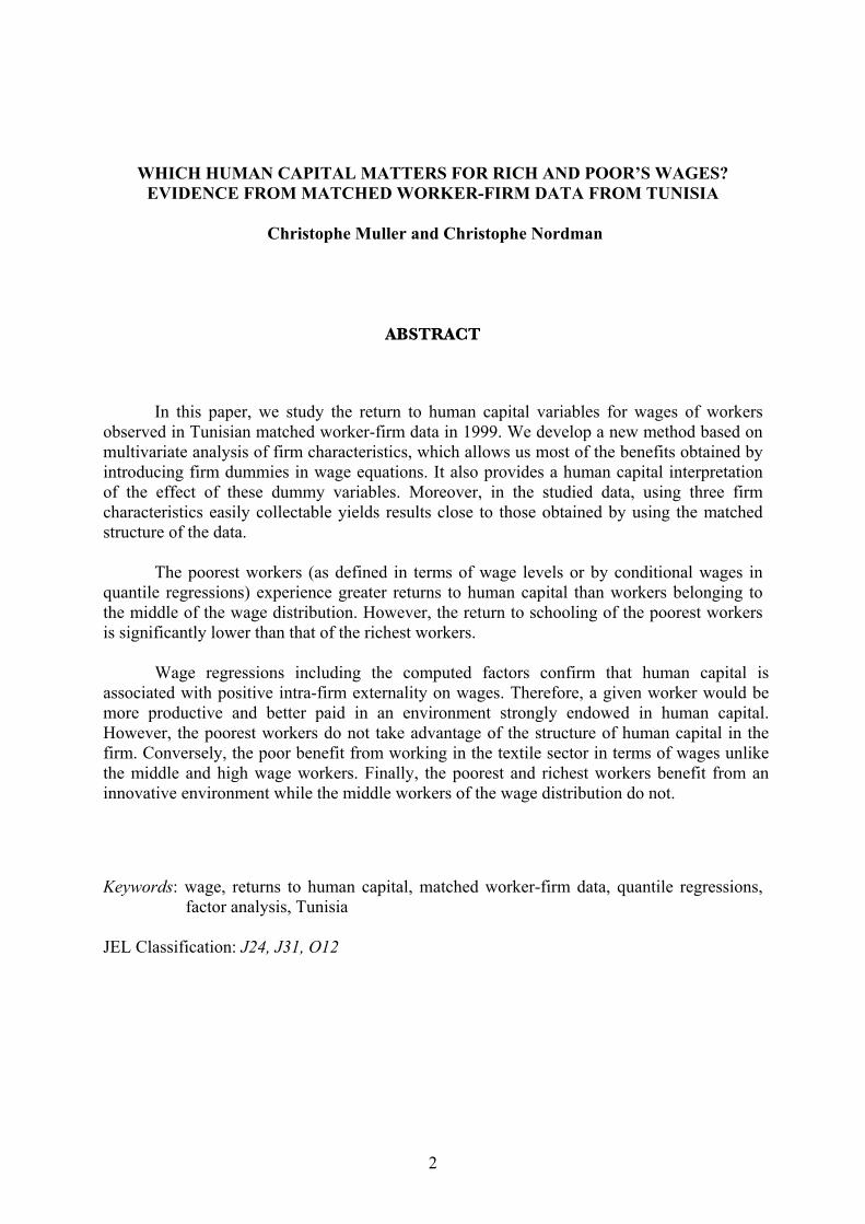
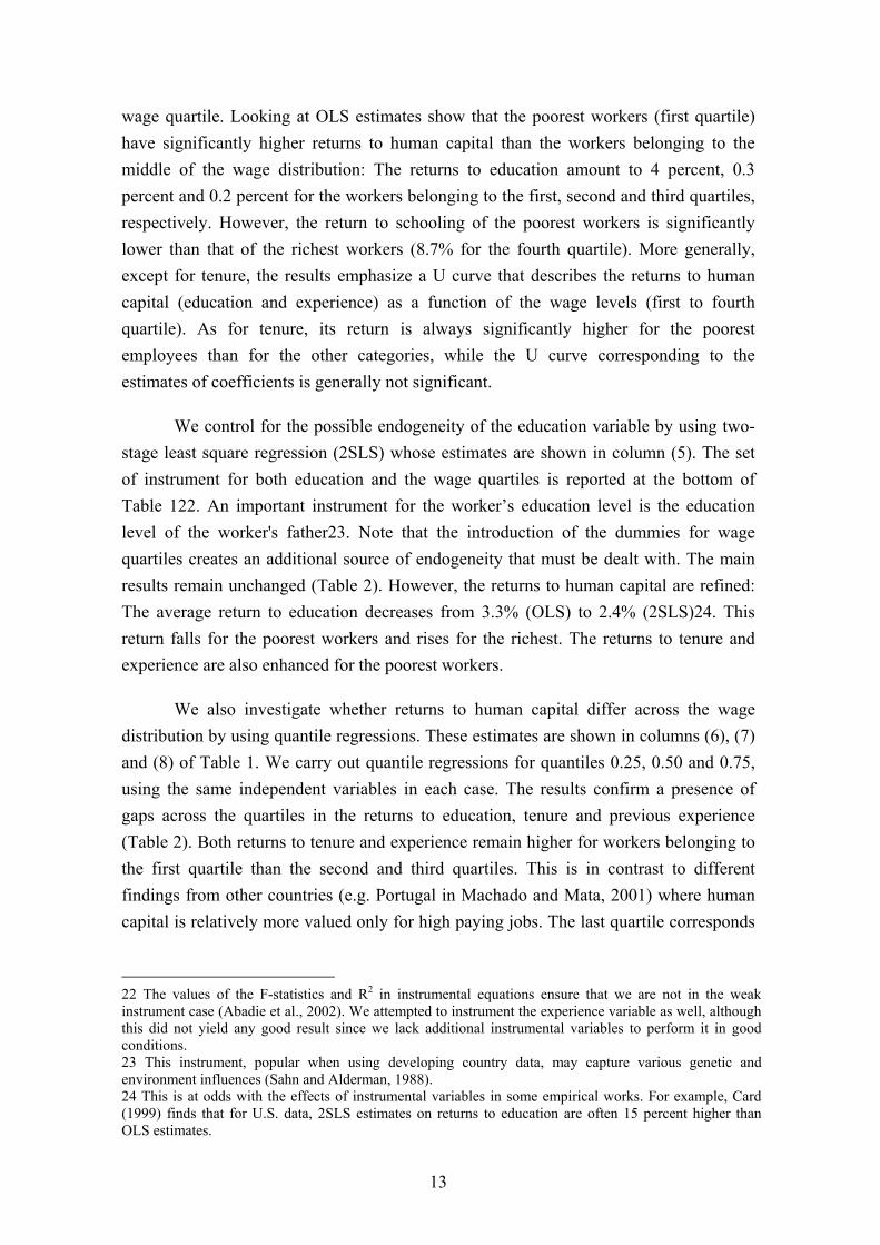
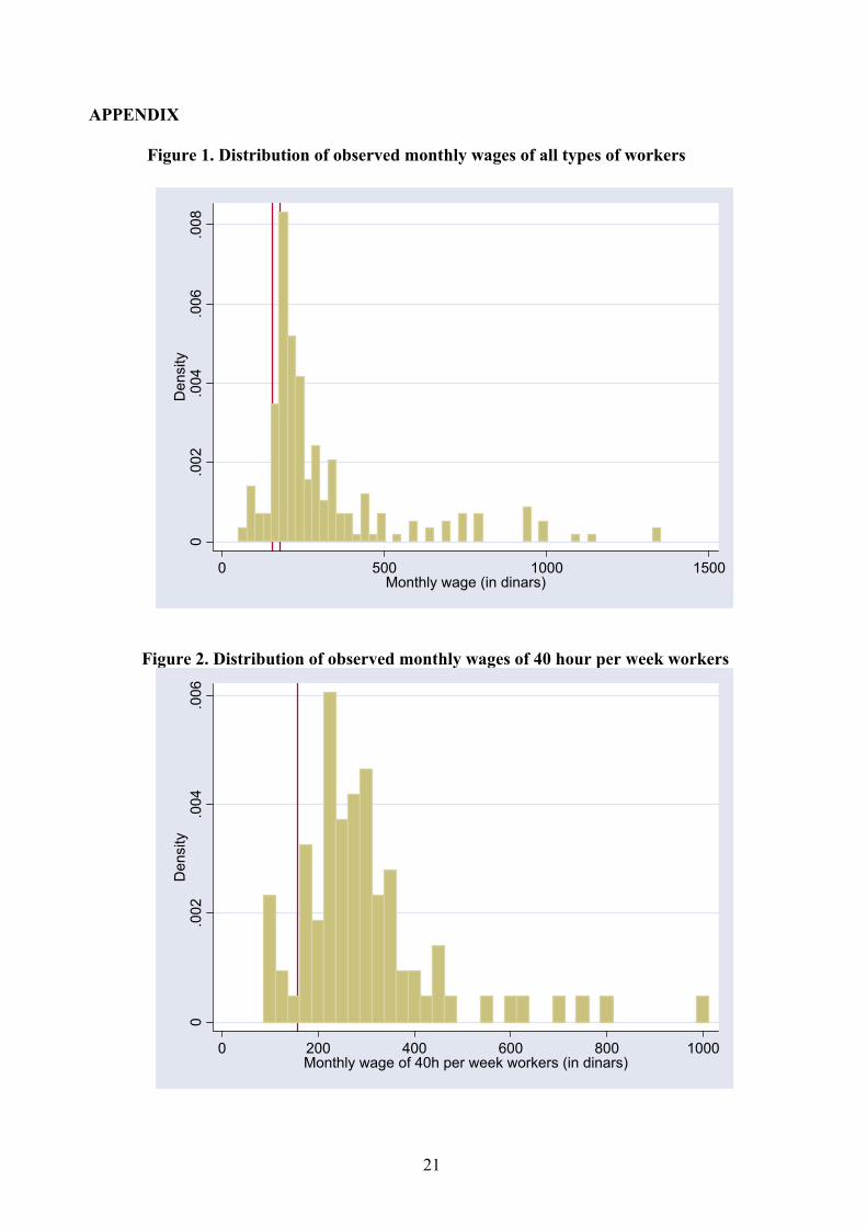
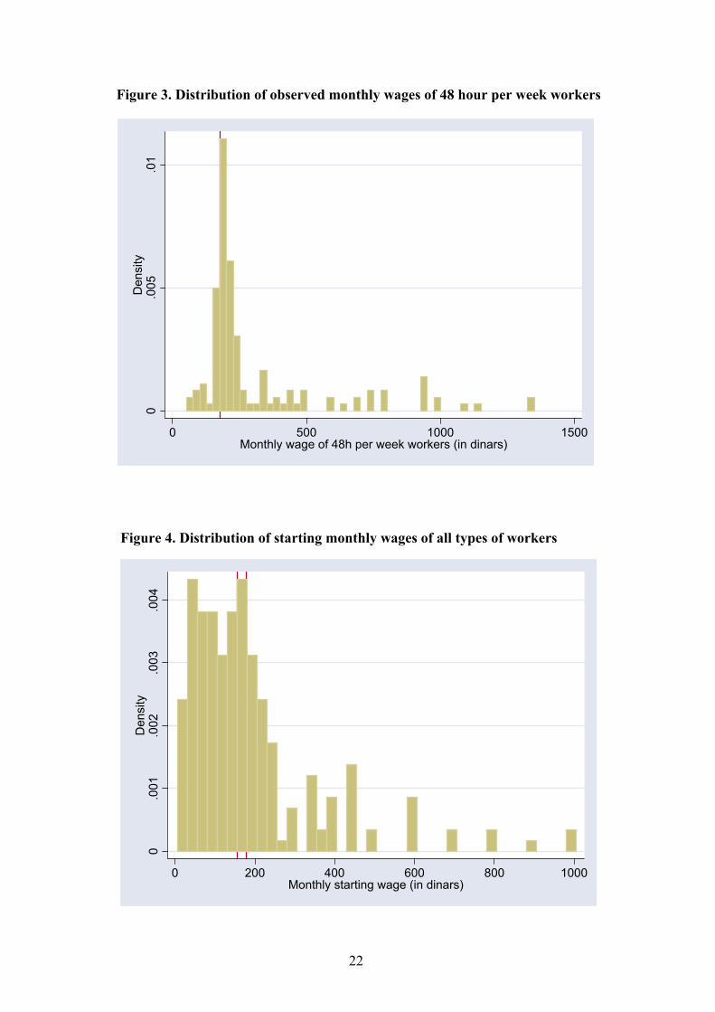
Information about the firm’s characteristics have been collected directly from the employers: composition of the workforce, work organization, training and communication policies, organizational or technical innovations and competitive situation of the firm. Table 7 in the Appendix shows descriptive statistics. Figures 1 to 4 in the Appendix show the histograms of initial wages and observed wages. The minimum wage are separately indicated by vertical lines for 40 hours a weeks and 48 hours a week, since different minimum wages are used for the two categories.
Contemporary wages are concentrated around values slightly above the minimum wage, while heavy right tails account for a small number of very skilled workers. Initial wages are also very concentrated, often below the present minimum wage. The latter feature is due to the minimum wage rise since the worker entered the firm, but also to workers paid below minimum wage. We are now ready to discuss the estimation results.
15 Low (high) skilled workers do not systematically correspond to low (high) pay workers. Another approach could have been to oppose skill categories rather than wage levels. In this paper, we focus on wage categories to capture differential social consequences of training and education policies. 16 The observed firms were selected among firms exporting their production and not with entirely foreign capital.

10
3. Estimation Results
3.1 The model and the estimation method
The matched worker-firm data enables us to estimate the returns of human capital using both workers’ and on their firms’ information. For this purpose, the Mincerian earnings function is a convenient tool for estimating the average returns to education and labour market experience. The return to education is given by the coefficient of schooling duration in the wage equation17. However, returns to human capital can vary across wage categories. For instance, high wage workers should not benefit from the same return to experience than low wage workers since the latter may have less incentives to make further on-the-job investment in human capital because they only deal with basic tasks. Alternatively, more educated individuals – generally with higher wages – may have greater incentive to invest in training because they learn more quickly. As a result, the shape of the relationship between the workers’ wage level and their returns to education and work experience (former experience plus tenure in the incumbent firm) is not clear. In order to capture differentiated returns of education and experience between the rich and the poor, we construct four individual dummies indicating the workers’ relative position in the sample in terms of hourly wage (quartile 1 to quartile 4). These dummies (QUARTILEi, i: 1…4) are allowed to interact with the main three human capital variables in the wage equation: education, tenure and previous work experience.
As alluded in the introduction, the lack of suitable matched firm-employee data for the wage analysis has been deplored by a number of authors, such as Rosen (1986) and Willis (1986), as such data allows the structure of wages to be modelled while controlling firm-specific effects. With our matched data, we can deal with the firm heterogeneity by introducing firm dummy variables into the wage equation. However, since we have cross-sectional data, we cannot model unobserved individual heterogeneity in the way of Abowd, Kramarz and Margolis (1999). To temper the effects of unobserved individual heterogeneity which might bias the estimated coefficients, we add control variables to our OLS regressions and also perform instrumented regressions (2SLS).
17 Quadratic and more flexible polynomial specifications have been tried but cannot be accurately estimated with these data.

11
Naturally, using firm dummies is a rough way of accounting for intra-firm human capital externalities. Meanwhile, it is possible that part of what could be interpreted as human capital externalities in the estimates is in fact a consequence of the worker selection by firms and vice versa. For example, very productive firms and workers may choose each other. In this paper, because of data limitations, we do not deal with this difficulty, and we assume that selectivity and sub-sampling effects can be neglected.
In the wage equations, we incorporate formal training received in the current firm (ongoing training and past training). In our sample, generally more educated workers receive more formal training: on average 12.2 years of schooling for workers having received formal training compared to 9.1 for the others.
Two other dummy variables are retained in the regressions18. One dummy variable controls for the worker’s hierarchical position in the firm (executive or supervisor) while the other takes into account the worker’s bargaining power within her firm (trade union membership). The worker’s relative hierarchical position is expected to have a positive effect on earnings differentials. The effect of union membership on wages remains unclear in the empirical literature.
We do not limit our analysis to the OLS results or 2SLS estimations. Introducing dummies for quartiles in the regressors creates endogeneity problems that may be imperfectly corrected with instrumental variable methods. A way to avoid this difficulty is by using quantile regressions. Quantile regression and least absolute deviation estimators have recently become very popular estimation methods (Koenker and Bassett, 1978), which have been employed for wage analyses (Buchinsky, 1998, 2001). This technique can be interpreted as the error distribution in the wage equation for the definition of different wage categories, instead of observed wage differentials. The popularity of these methods relies on two sets of properties. First, they provide robust estimates, particularly for misspecification errors related to non-normality and heteroscedasticity, but also for the presence of outliers, often due to data contamination. Second, they allow the researcher to concentrate her attention on specific parts of the distribution of interest. This is the case when the distribution of interest is the conditional distribution of the dependent variable.
Moreover, focusing on the quantiles of error terms in wage equations, introduces an alternative notion of wage precariousness that can be contrasted with the quantiles of the wage distribution. One can oppose the low observed level of wages in OLS and 2SLS estimates with the low conditional wage level in the quantile regression estimates.
18 All the other socio-economic variables such as sex, matrimonial status and geographic origin are dropped from the regressions for lack of significance and to preserve degrees of freedom.

12
We choose to pursue these two approaches. We find that the residuals’ quartiles from the quantile regressions are correlated to those obtained when different quartiles are used to define the quantile regression. In contrast, they are not as strongly correlated to the quartiles of the wages themselves. Thus, the low quantiles corresponding to the two approaches capture distinct descriptions of wage precariousness.
Finally, bootstrap confidence intervals are used for quantile regressions in order to avoid the consequences of the slow convergence of classical confidence intervals of estimates (Hahn, 1995). Let us examine the estimates.
3.2 The wage equation estimates
Our first estimates of the equations of the logarithm of individual hourly wage are reported in Table 1 of the Appendix. The first two columns correspond to OLS estimates without wage quartiles as regressors. The following two columns show the results obtained when the returns to human capital can vary across wage quartiles through the inclusion of dummy variables for wage quartiles19.
The wage equation which incorporates firm’s fixed effect is characterized by a better goodness-of-fit than the standard Mincerian wage function20. As noticed by Abowd and Kramarz (1999), the return to schooling decreases after controlling for firms’ heterogeneity with fixed effects. In OLS regressions, the marginal return to education in Tunisia is 6.9 percent with the firm’s fixed effects instead of 8.6 percent without the firm dummies. To our knowledge, no comparable estimates exist on Tunisia21.
Columns (3) and (4) elicit returns to human capital that are significantly different across wage quartiles, without and with adding the firm’s fixed effect, respectively. Table 2 summarizes the main results of all these estimators by computing the coefficients of the returns to education, to job tenure and to previous experience for each 19 We also test interactions of these dummies with the quadratic terms of experience variable to take into account possible differentiated decreasing returns to experience across wage quartiles. However, since the results were not very convincing, we choose to exclude these interactions to preserve on degrees of freedom. 20 The Fisher test of the constrained model (without the firm’s fixed effect) against the unconstrained model (fixed effects) shows that we cannot reject the unconstrained model at the 1 percent level. 21 See Psacharopoulos (1985, 1994, 2002) for surveys reporting the returns to education in numerous countries. Some of the education effect may be caused by selection. Firm dummies may help control for the selection effects, but other individual and household characteristics are missing which does not allow us to be fully protected against a selectivity bias.
13
wage quartile. Looking at OLS estimates show that the poorest workers (first quartile) have significantly higher returns to human capital than the workers belonging to the middle of the wage distribution: The returns to education amount to 4 percent, 0.3 percent and 0.2 percent for the workers belonging to the first, second and third quartiles, respectively. However, the return to schooling of the poorest workers is significantly lower than that of the richest workers (8.7% for the fourth quartile). More generally, except for tenure, the results emphasize a U curve that describes the returns to human capital (education and experience) as a function of the wage levels (first to fourth quartile). As for tenure, its return is always significantly higher for the poorest employees than for the other categories, while the U curve corresponding to the estimates of coefficients is generally not significant.
We control for the possible endogeneity of the education variable by using two-stage least square regression (2SLS) whose estimates are shown in column (5). The set of instrument for both education and the wage quartiles is reported at the bottom of Table 122. An important instrument for the worker’s education level is the education level of the worker's father23. Note that the introduction of the dummies for wage quartiles creates an additional source of endogeneity that must be dealt with. The main results remain unchanged (Table 2). However, the returns to human capital are refined: The average return to education decreases from 3.3% (OLS) to 2.4% (2SLS)24. This return falls for the poorest workers and rises for the richest. The returns to tenure and experience are also enhanced for the poorest workers.
We also investigate whether returns to human capital differ across the wage distribution by using quantile regressions. These estimates are shown in columns (6), (7) and (8) of Table 1. We carry out quantile regressions for quantiles 0.25, 0.50 and 0.75, using the same independent variables in each case. The results confirm a presence of gaps across the quartiles in the returns to education, tenure and previous experience (Table 2). Both returns to tenure and experience remain higher for workers belonging to the first quartile than the second and third quartiles. This is in contrast to different findings from other countries (e.g. Portugal in Machado and Mata, 2001) where human capital is relatively more valued only for high paying jobs. The last quartile corresponds
22 The values of the F-statistics and R2 in instrumental equations ensure that we are not in the weak instrument case (Abadie et al., 2002). We attempted to instrument the experience variable as well, although this did not yield any good result since we lack additional instrumental variables to perform it in good conditions. 23 This instrument, popular when using developing country data, may capture various genetic and environment influences (Sahn and Alderman, 1988). 24 This is at odds with the effects of instrumental variables in some empirical works. For example, Card (1999) finds that for U.S. data, 2SLS estimates on returns to education are often 15 percent higher than OLS estimates.

14
to the highest returns to education. However, the differences across the workers’ categories are smaller than those for the OLS and 2SLS.
Let us now look at the other estimated coefficients. Completed formal training plays an important role in explaining wage differentials (its coefficient is always significant at a 5 percent level and positive). This is consistent with theories that argue that wage differentials should reflect differences in training investments. On the other hand, the negative coefficient of the ongoing formal training variable, although not always significant, is consistent with Becker’s (1975) prediction that the costs of general training are shared between employers and employees (also found in Barron et al., 1998). If this formal training is of general content, then the workers should partly compensate for it by accepting a lower wage during the training period. As shown by the estimates, they ultimately benefit from this training which provides them with a positive wage premium (from 10 percent to 30 percent increase depending on the regression) when the training is completed.
Finally, the estimates of the firm dummies’ coefficients are systematically large and significant at the 1 percent level. This is in accordance with the usual persistence of wage differentials across individuals with identical productive characteristics in empirical studies25. Such wage differentials have been found in Tunisia in non-matched data (Abdennadher et al., 1994). The results show that workers with comparable measured characteristics can earn very different wages because they belong to different firms. In this study, wage differentials across firms will receive further consideration in the next sub-section with an interpretation of the firm effect on individual earnings in terms of each company’s organizational features.
3.3 Factor analysis of the firm’s characteristics
We use a method of factor analysis, the principal component analysis, to summarize the information about the surveyed firms26. This method is based on the calculation of the inertia axes in a cloud of points that represents data in table format. For our purpose, the first three estimated factors concentrate most of the relevant
25 See Krueger and Summers (1988), Abowd, Kramarz and Margolis (1999) and Goux and Maurin (1999). 26 In principal component analysis, a set of variables is transformed into orthogonal components, which are linear combinations of the variables and have maximum variance subject to being uncorrelated with one another. Typically, the first few components account for a large proportion of the total variance of the original variables, and hence can be used to summarize the original data.

15
information about the firm’s characteristics. In a sense, we generalize the approach by Cardoso (1998) who regresses the firms’ fixed effects on different variables.
Table 3 shows the results of the principal component analysis, with the definition of the main three inertia axes (the factors), which are linear components of the firm’s characteristics used for the analysis. The other factors represent a negligible amount of statistical information and are dropped from the analysis. In our basic specification without quartile dummies, OLS estimates without the firm’s dummies nor factors enable us to explain 67 percent of the log-wages variance. Adding our three factors raises this proportion by 8 percent, and the firm’s dummies instead by 9 percent only. The correlation coefficients of these characteristics with the first three factors are indicated for the interpretation. Clearly, the first factor corresponds to the activity sector (textile against IMMEE). The second factor describes the ‘density in the firm’ of the human capital characteristics. The third factor is closely associated with the firm’s modern features.
Table 4 indicates the correlation coefficients of the first three factors with the firm dummies on one hand, and a few education and gender characteristics of workers in the firm on the other hand. They confirm common wisdom about how the firm is characterized by each factor. Firms in the textile sector have a higher proportion of female workers and less educated or trained workers. Firms with high human capital density exhibit higher average education levels. Modern firms invest more in formal training.

16
3.4 Wage equations with firm factors
The factor analysis enables us to summarize the main information on the firms' characteristics into three principal components (factors)27. By contrast with the firms’ fixed effects introduced in the wage regressions in Table 1, the three factors suggest qualitative characteristics of the firms. In Table 5, we estimate the same wage equations in which the firm fixed effects are replaced by the three factors.
The first column reports the OLS estimates. The coefficient of the first factor, reflecting the industrial sector (positively correlated with the textile sector), is statistically significant at 5 percent level and has a negative sign. This is consistent with the fact that in Tunisia the textile sector is the manufacturing industry with the lowest wage. Ceteris paribus, workers belonging to this sector experience a lower wage.
The second factor has a significant positive impact on wage differentials (at 1 percent). Since Factor 2 reflects the density of each firm’s human capital, this result may suggest that the firm’s human capital generates positive wage externality. A worker with a given skill would be more productive and thus, better paid in an environment highly endowed in human capital. The third factor, reflecting the firm’s age and its capacity to promote innovations and new technology has no significant effect in this specification.
In the following two regressions (columns 2 and 3), we add the wage quartile dummies and allow them to interact with the three factors in order to identify if differentiated effects of factors and variables exist across wage groups. The factors’ main results are also reported in Table 2.
First, from the OLS regression, it appears that the poorest workers (first quartile) benefit from working in the textile sector unlike medium and high-wage workers. Second, the poorest workers do not seem to take advantage of the firm’s human capital since they experience a negative impact on their wages from Factor 2. This result may reflect differences in bargaining power within firms across wage groups, or be associated with differences in the human capital role in the undertaken tasks across wage groups. It could also be interpreted in terms of knowledge diffusion. The transmission of knowledge might be reserved only for high wage or high skilled workers. Also, the correlation coefficient of Factor 2 with the importance of supervision is 0.98, while it is 27 Various studies tried to separate the external effects of the group or the sector in which the workers evolve from the purely individual effects on their earnings differentials. Mean variables were added in earnings functions, after a control for the individual characteristics, by Dickens and Katz (1987), Krueger and Summers (1988), Blanchflower and Oswald (1994), Chennouf, Lévy-Garboua and Montmarquette (1997) and Kölling, Schnabel and Wagner (2002). Using factors is a further step in this direction.

17
0.96 with the managerial/staff proportion. Then the negative effect of Factor 2 on the first quartile wage may result from the fact that excessive supervision prevents development of human capital externalities because it limits individual responsibility and promotion possibilities. The richer and more qualified social categories are the ones who benefit the most from the firm’s human capital density. As for Factor 3 (modernity of the firm), its impacts on wages emphasizes the same U curve as described earlier for the returns to human capital across wage groups. The poorest and richest workers benefit from an innovating environment, while workers in the middle of the wage distribution do not.
The results with 2SLS and quantile regressions show similar features for the positive effect of the second factor. However, as expected, because of the accuracy lost in the instrumentation, the coefficient of the various equations incorporating factor dummies are often non-significant with the 2SLS, particularly when factor dummies are interacted with quartile dummies. Finally, the quantile regression estimates of factor effects are different in that they are not based on many interacted effects of factors and quartiles, but only on one coefficient for each selected factor. In this case, the first factor (textile) corresponds to a significant negative effect, the second factor to a significant positive effect, while factor 3 has no significant impact. These results illustrate the differences in the two notions of wage positions, respectively based on wage quantiles or wage conditional quantiles. These two notions are associated with the factors’ different impacts.
Finally, we carry out a simple regression by replacing the three factors with three of the firm’s characteristics that seem to be better reflecting each of them: a dummy for the textile sector (Factor 1), the average education level in the firm (Factor 2) and the firm’s age (Factor 3). Using a questionnaire addressed to workers (e.g. during an employment survey or a labor force survey), it would be easy to collect information on these three characteristics (sector, proxy of average education in this firm, age of this firm) and use them afterwards as regressors in the wage equation. We call this regression the "pseudo factor" model (PFM, column 4 of Table 5). The coefficients of the three selected variables are statistically significant at 1 percent and have the expected sign. It is interesting to compare the estimators obtained from this regression to those drawn from a simple Mincerian model (MM) and a firm fixed effects model (FFEM) (Columns 1 and 2 in Table 1). Clearly, it appears that the PFM does very well compared to the FFEM: the returns to human capital obtained from the PFM are closer to those of the FFEM than to the same returns drawn from the MM. More specifically, the PFM gives a return to education similar to that obtained by the FFEM (6.8 percent compared to 6.9 percent with the FFEM, while it amounts to 8.6 percent with the MM).

18
On one hand, the comparison of estimation results with the firms’ fixed effects with estimation results with factor effects on the other hand is instructive. Indeed, the firms’ fixed effects could be partly interpreted as resulting from unobserved human capital characteristics at the firm’s level. Under such assumption, the estimation results show that in our data three of the firm’s observable characteristics suffice to account for most of the impact of the firm’s effects on wages. As a consequence, the technique proposed in this paper to take advantage of matched worker-firm data could also be useful for other applied research when matched worker-firm data are not available.
We obtained returns to education in the equations without the firm’s characteristics that are substantially different from the returns to education in equations with the firm’s fixed effects. As in Chennouf et al. (1997) for Algeria, the returns to education diminish when the firm’s effects are introduced. However, this only occurs when all quarters are considered together. The results also show it is important to consider the different quartiles of the wage distribution.
Meanwhile, the returns to education obtained with the firm’s fixed effects are almost indistinguishable from the returns in equations with factors, and from the returns in equations with mean education characteristics of the firms. This suggests that the firm’s effects can be corrected by introducing these mean education characteristics if the main interest is to estimate returns to education.
Finally, the introduction of factors may be used to better interpret the firm dummies in equation with the firms’ fixed effects. For example, the characteristics of firm number 1 (respectively firm number 6, respectively firm number 7) are very close to that of Factor 1, ‘textile type industry’ (respectively Factor 2, ‘high qualification’, respectively Factor 3, ‘modern firm’).
4. Conclusion
In this paper, we study the return to human capital variables for wages of workers observed in Tunisian matched worker-firm data in 1999. We also develop a new method based on multivariate analysis of firm characteristics. This method allows us most of the benefits obtained by introducing firm dummies in wage equations. It also provides a human capital interpretation of the effect of these dummy variables. Moreover, in the studied data, using three firm characteristics easily collectable (average education level

19
of workers, sector, age of the firm) yields results close to those obtained by using the matched structure of the data.
The results show wage equations incorporating the firms’ fixed effects have a better fit than the standard Mincerian wage functions. All the wage equations show large effects from the firm dummies. This is consistent with the persistence of wage differentials across individuals with identical productive characteristics.
With or without controlling for firm characteristics and for possible endogeneity of the education variable, the poorest workers (as defined in terms of wage levels or conditional wages in quantile regressions) experience greater returns to human capital than workers belonging to the middle of the wage distribution. However, the return to schooling of the poorest workers is significantly lower than that of the richest workers.
The impact of formal job training on earnings is consistent with general predictions of human capital theory: individuals are assumed to invest in training during an initial period and receive a lower wage than what they could receive elsewhere during training. Workers may collect returns from their investment at a later period through higher marginal products and higher wages.
Using a factor analysis to summarize the information on the surveyed firm, we show the activity sector of the firm, its human capital characteristics and modern features concentrate most of the statistical information from the employer survey.
Wage regressions, including the computed factors, confirm that human capital seems to constitute a source of positive intra-firm externality on wages. A given worker would be more productive and better paid in an environment strongly endowed in human capital. However, the poorest workers do not take advantage of the structure of human capital in the firm. Conversely, the poor benefit from working in the textile sector in terms of wages unlike the medium and highly paid workers. Finally, the poorest and richest workers benefit from an innovating environment while workers in the middle of the wage distribution do not.
An alternative interpretation is that the estimated intra-firm externality on wages partially captures the role of unobserved physical capital. Indeed, it may be that high human capital and training are correlated with high capitalistic intensity across firms. If that is the case, the impacts of human and physical firm capital on wages should be analyzed jointly. This calls for accurate measurement of these two types of variables, notoriously hard to observe.

20
What are the policy implications? In the Tunisian context, emerging tensions in the labor market – resulting from uncertainty about job tenure and deterioration in relative wages for lower-skilled workers – will need to be closely followed through comprehensive monitoring of unemployment, skill composition and location. The role of education and formal training is central in dealing efficiently with these tensions. One of the outcomes of the estimations is that human capital investment should partly proceed through the work organization and training policy of the firm and not only stem from public education policies.
Moreover, poverty in Tunisia has been found to be more concentrated in the textile sector among manufacturing sectors. This is consistent in our data with lower wages observed in the textile sector. However, it is interesting to observe that the return to human capital is particularly high for the poorest workers in this industry. Then, this sector can play a role of skill promoter for low-skilled manpower. Once these workers in this type of industry have raised their productivity by a work period, they may be able to switch to another activity sector in search of better remunerations, although we cannot test this hypothesis with our data.
Finally, what can we expect from public policies using education as an instrument to fight poverty and inequality? The U-curve of the returns to the different human capital variables as a wage function implies that human capital accumulation is likely to help alleviate poverty but may have ambiguous effects on inequality. This makes it all the more worrying that Mesnard and Ravallion (2001) found raising inequality depletes the aggregate number of business starts-up, and therefore may reduce future economic growth. In these conditions, welfare public programs based on reinforcement of workers’ skills and knowledge should be accompanied by monitoring benefits that every society class would receive from education and training, including that in the workplace itself.
21
APPENDIX
Figure 1. Distribution of observed monthly wages of all types of workers
0.0
02.0
04.0
06.0
08D
ensi
ty
0 500 1000 1500Monthly wage (in dinars)
Figure 2. Distribution of observed monthly wages of 40 hour per week workers
0.0
02.0
04.0
06D
ensi
ty
0 200 400 600 800 1000Monthly wage of 40h per week workers (in dinars)
22
Figure 3. Distribution of observed monthly wages of 48 hour per week workers
0.0
05.0
1D
ensi
ty
0 500 1000 1500Monthly wage of 48h per week workers (in dinars)
Figure 4. Distribution of starting monthly wages of all types of workers
0.0
01.0
02.0
03.0
04D
ensi
ty
0 200 400 600 800 1000Monthly starting wage (in dinars)

23
Table 1. Wage equations Dependent variable: Log hourly wage (lnsalh)
OLS OLS OLS OLS IV (2SLS)
Quantile regressions (bootstrap standard error: 20 iterations)
Firm fixed effects models
Explanatory variables
(1)
Firm fixed effects model
(2)
(3)
Firm fixed effects model
(4)
Firm fixed effects model
(5)
0.25 Quantile
(6)
0.50 Quantile
(7)
0.75 Quantile
(8)
Constant -0.7324*** (0.0864)
0.00 0.0090 (0.1275)
0.94 -0.1616 (0.2186)
0.46 -0.0459 (0.2093)
0.82 -0.1034 (0.4177)
0.81 0.2098 (0.3110) 0.50 0.5531**
(0.2798) 0.04 0.2570 (0.2652) 0.33
Education 0.0861*** (0.0071) 0.00 0.0691***
(0.0068) 0.00 0.0857*** (0.0103) 0.00 0.0870***
(0.0124) 0.00 0.0915*** (0.0248) 0.00 0.0498***
(0.0114) 0.00 0.0448*** (0.0156) 0.00 0.0686***
(0.0157) 0.00
QUARTILE1 _ _ -0.5933** (0.2369) 0.01 -0.3702
(0.2271) 0.10 -0.4284 (0.4424) 0.33 _ _ _
QUARTILE2 _ _ 0.2733 (0.2365) 0.25 0.5047**
(0.2268) 0.02 1.0567* (0.5536) 0.06 _ _ _
QUARTILE3 _ _ 0.6223*** (0.2353) 0.01 0.7992***
(0.2253) 0.00 0.7524 (0.4845) 0.12 _ _ _
Education*QUARTILE1 _ _ -0.0433***(0.0159) 0.01 -0.0464***
(0.0152) 0.00 -0.0596* (0.0335) 0.08 _ _ _
Education*QUARTILE2 _ _ -0.0809***(0.0154) 0.00 -0.0839***
(0.0146) 0.00 -0.1286***(0.0363) 0.00 _ _ _
Education*QUARTILE3 _ _ -0.0814***(0.0147) 0.00 -0.0848***
(0.0139) 0.00 -0.0806***(0.0293) 0.01 _ _ _
Tenure 0.0255** (0.0107) 0.02 0.0452***
(0.0099) 0.00 -0.0071 (0.0085) 0.41 0.0099
(0.0087) 0.25 0.0107 (0.0160) 0.50 0.0448**
(0.0233) 0.05 0.0271** (0.0141) 0.05 0.0362***
(0.0122) 0.00
Tenure2 -0.0004 (0.0005) 0.43 -0.0012***
(0.0004) 0.01 0.0006** (0.0003) 0.05 0.0002
(0.0003) 0.54 0.0002 (0.0005) 0.76 -0.0009
(0.0009) 0.33 -0.0006 (0.0006) 0.34 -0.0008*
(0.0005) 0.10
Tenure*QUARTILE1 _ _ 0.0699*** (0.0128) 0.00 0.0621***
(0.0130) 0.00 0.0755** (0.0339) 0.03 _ _ _
Tenure*QUARTILE2 _ _ 0.0022 (0.0091) 0.81 -0.0094
(0.0090) 0.29 -0.0362 (0.0276) 0.19 _ _ _
Tenure*QUARTILE3 _ _ -0.0015 (0.0062) 0.81 -0.0091
(0.0062) 0.14 -0.0085 (0.0135) 0.53 _ _ _
Experience 0.0325*** (0.0127) 0.01 0.0426***
(0.0117) 0.00 0.0373*** (0.0103) 0.00 0.0495***
(0.0102) 0.00 0.0426*** (0.0171) 0.01 0.0467**
(0.0233) 0.04 0.0306** (0.0148) 0.04 0.0322**
(0.0166) 0.05
Experience2 -0.0004 (0.0007) 0.57 -0.0011*
(0.0006) 0.10 -0.0006
(0.0004) 0.20 -0.0009** (0.0004) 0.03 -0.0005
(0.0006) 0.40 -0.0015 (0.0016) 0.33 -0.0010
(0.0008) 0.24 -0.0002 (0.0012) 0.87
Experience*QUARTILE1 _ _ 0.0057 (0.0130) 0.66 -0.0022
(0.0127) 0.86 0.0274 (0.0344) 0.43 _ _ _
Experience*QUARTILE2 _ _ -0.0290***(0.0083) 0.00 -0.0345***
(0.0079) 0.00 -0.0512***(0.0168) 0.00 _ _ _
Experience*QUARTILE3 _ _ -0.0270***(0.0082) 0.00 -0.0347***
(0.0079) 0.00 -0.0324** (0.0150) 0.03 _ _ _
Ongoing formal training -0.4972*** (0.1798) 0.00 -0.4159***
(0.1577) 0.01 -0.1542 (0.1001) 0.13 -0.1288
(0.0948) 0.17 -0.0821 (0.1211) 0.50 -0.3502
(0.2522) 0.16 -0.4649** (0.2236) 0.04 -0.3384
(0.2501) 0.17

24
Completed formal training 0.4885*** (0.0660) 0.00 0.2710***
(0.0735) 0.00 0.2103*** (0.0384) 0.00 0.1313***
(0.0445) 0.00 0.1107** (0.0547) 0.04 0.3275**
(0.1433) 0.02 0.2270** (0.0961) 0.02 0.1853*
(0.1007) 0.06
Union -0.0835 (0.0649) 0.19 0.0012
(0.0619) 0.99 -0.0715* (0.0403) 0.08 -0.0573
(0.0401) 0.15 -0.0434 (0.0559) 0.44 -0.0030
(0.1023) 0.97 0.0884 (0.0696) 0.20 0.0373
(0.1113) 0.73
Executive or supervisor 0.2124*** (0.0698) 0.00 0.2655***
(0.0618) 0.00 0.0940** (0.0395) 0.02 0.1272***
(0.0384) 0.00 0.1264*** (0.0480) 0.01 0.1941**
(0.0824) 0.02 0.3436*** (0.0764) 0.00 0.2889***
(0.0861) 0.00
Firm1 _ -0.5318***(0.1041) 0.00 _ -0.2797***
(0.0679) 0.00 -0.2460***(0.0890) 0.01 -0.7944***
(0.2545) 0.00 -0.8185***(0.1240) 0.00 -0.6331***
(0.2587) 0.01
Firm2 _ -0.4824***(0.1019) 0.00 _ -0.3066***
(0.0651) 0.00 -0.2877***(0.0865) 0.00 -0.6706***
(0.2293) 0.00 -0.7262***(0.1503) 0.00 -0.5229***
(0.1752) 0.00
Firm3 _ -0.7895***(0.1033) 0.00 _ -0.3567***
(0.0680) 0.00 -0.3002***(0.0904) 0.00 -0.9655***
(0.2586) 0.00 -1.0392***(0.1550) 0.00 -0.8133***
(0.1766) 0.00
Firm4 _ -0.7425***(0.1082) 0.00 _ -0.3745***
(0.0716) 0.00 -0.3208***(0.1012) 0.00 -0.9637***
(0.2648) 0.00 -0.9987***(0.1995) 0.00 -0.8391***
(0.1962) 0.00
Firm5 _ -0.7227***(0.1055) 0.00 _ -0.4016***
(0.0682) 0.00 -0.3643***(0.0953) 0.00 -0.9420***
(0.2426) 0.00 -0.9317***(0.1855) 0.00 -0.7328***
(0.1602) 0.00
Firm7 _ -0.6098***(0.1036) 0.00 _ -0.3015***
(0.0701) 0.00 -0.2852***(0.0946) 0.00 -0.7814***
(0.2368) 0.00 -0.6602***(0.1522) 0.00 -0.6072***
(0.1134) 0.00
Firm8 _ -0.7736***(0.1007) 0.00 _ -0.3297***
(0.0667) 0.00 -0.2473***(0.0909) 0.01 -0.9083***
(0.2455) 0.00 -0.9900***(0.1611) 0.00 -0.7999***
(0.1902) 0.00
R2 0.67 0.76 0.91 0.92 0.905 Pseudo R2
0.43 Pseudo R2
0.54 Pseudo R2
0.61 Observations 231 231 231 231 231 231 231 231
Standard errors are given in parentheses. P-values appear in italic. ***, ** and * mean respectively significant at the 1%, 5% and 10% levels. Instrumented: Education QUARTILE1 QUARTILE2 QUARTILE3 Education*QUARTILE1 Education*QUARTILE2 Education*QUARTILE3 Tenure*QUARTILE1
Tenure*QUARTILE2 Tenure*QUARTILE3 Experience*QUARTILE1 Experience*QUARTILE2 Experience*QUARTILE3 Instruments: age, (age)2, apprenti, celibah, chaine, choma, (choma)2, choma*female, emsim, enft, (enft)2, log(enft), enft*age, entree, equipe, formaa, (formaa)2,
(formaa)3, formaa*female, forstil*female, mari*female, mari*female, mari*male, panal, panal*age, panal*choma, panal*enft, panal*formaa, pprim, pprim*age, pprim*choma, pprim*enft, pprim*formaa, prove, psecon, psecon*age, psecon*choma, psecon*enft, psecon*formaa, psup, psup*age, psup*choma, psup*enft, psup*formaa, staga, (staga)2, (staga)3, stagan, (stagan)2, (stagan)3.
The definitions of the variables and instruments appear in appendix, Table 6.

25
Table 2. Returns to human capital and wage effects of factors on quartiles
OLS 2SLS Quantile regressions Quartiles Quartiles
1st 2nd 3rd 4th meanb 1st 2nd 3rd 4th meanb 0.25
Quantile0.50
Quantile0.75
Quantile Independent variables Firm fixed effects models
Education 0.0405 0.0031 0.0022 0.0870 0.0330 0.0318 -0.0371 0.0108 0.0915 0.0240 0.0498 0.0448 0.0686
Tenurea 0.0621 0.0027ns 0.0031ns0.0121ns 0.0231 0.0755 -0.0237ns0.0040ns0.0125ns 0.0203 0.0448 0.0271 0.0266
Experiencea 0.0414 0.0091 0.0088 0.0435 0.0256 0.0700 -0.0087 0.0102 0.0426 0.0285 0.0467 0.0306 0.0322
Factors effects models
Factor 1 0.0205 -0.0131
nd -0.0128
nd -0.0175 -0.0166 -0.0363ns
0.0285
ns 0.0001
ns 0.0127
ns -0.0049
ns -0.0544 -0.0561 -0.0360
Factor 2 -0.0935 -0.0014
nd 0.0114 0.0506 0.0392 0.3382
nd -0.3171 0.0206
nd 0.0318 0.0324 0.1026 0.1020 0.0764
Factor 3 0.0112 -0.0190 -0.0134 0.0295 -0.0014
ns -0.0296
nd 0.0179
nd -0.0347 0.0774 0.0050 -0.0121 ns -0.0099 ns -0.0113 ns a : returns calculated at the average point of the sub-sample. b : mean of the effects for the different quartiles. ns : no significantly different from zero at 10% level.
nd : no significantly different from the coefficient of the 4th quartile at 10% level.

26
Table 3. Principal component analysis
Firm characteristics Vectors Correlations Factor 1 Factor 2 Factor 3 Factor 1 Factor 2 Factor 3 Average human capital of employees in the firm Average age -0.269 -0.075 0.006 -0.75* -0.20 0.01 Average education -0.079 0.319 -0.196 -0.22 0.86* -0.33 Average tenure -0.226 -0.205 0.049 -0.63* -0.55 0.08 Average total experience -0.219 -0.237 0.133 -0.61 -0.64* 0.23 Variance of education 0.012 -0.268 0.091 0.03 -0.73* 0.15 Variance of tenure -0.278 -0.196 -0.049 -0.78* -0.53 -0.08 Variance of total experience -0.316 -0.140 -0.110 -0.88* -0.38 -0.19
General characteristics of the firm Sector (1: textiles; 0: IMMEE) 0.319 -0.107 0.112 0.89* -0.29 0.19 Size (number of employees) 0.219 -0.054 -0.144 0.61 -0.14 -0.24 Exportation (1: yes; 0: no) 0.254 0.152 -0.156 0.71* 0.41 -0.26 Percentage of exported production 0.331 0.041 0.082 0.93* 0.11 0.14 Level of competition (1 to 5) 0.302 -0.141 -0.128 0.85* -0.38 -0.22 Firm age 0.062 -0.074 -0.554 0.17 -0.20 -0.95* Rate of supervision -0.165 0.319 -0.058 -0.46 0.86* -0.10 Rate of management -0.051 0.355 0.061 -0.14 0.96* 0.10 Number of intermediary levels of management -0.025 -0.303 -0.086 -0.07 -0.82* -0.15 Existing system of formal training (1: yes; 0: no) -0.225 0.198 0.255 -0.63* 0.54 0.44 Organisational innovation the last four years (1: yes; 0: no) 0.049 0.085 0.332 -0.08 0.39 0.71*
Technological innovation the last four years (1: yes; 0: no) -0.029 0.143 0.415 0.14 0.23 0.57
Level of stimulated internal communication (1 to 3) -0.128 0.267 -0.157 -0.36 0.72* -0.27
Characteristics of employees’ tasks Work independence stimulated (1: yes; 0: no) 0.076 0.233 -0.097 0.21 0.63* -0.17 Frequent work control (1: yes; 0: no) 0.039 0.177 -0.194 0.11 0.48 -0.33 Versatility system implemented (1: yes; 0: no) 0.156 0.100 0.234 0.44 0.27 0.40 Percentage of employees working in chain 0.293 -0.097 0.205 0.82* -0.26 0.35 Task definition (1: globally defined; 0: precisely defined) -0.088 0.195 -0.010 -0.25 0.53 -0.02
*: significant at the 10% level.

27
Table 4. Correlations between factors, firm fixed effects and characteristics of education in the firms
*: significant at the 10% level .
Factor 1 Factor 2 Factor 3 Firms’ fixed effects
Firm 1 -0.72* -0.26 0.47 Firm 2 -0.21 -0.27 -0.12 Firm 3 0.38 -0.04 0.47 Firm 4 0.32 -0.07 0.03 Firm 5 0.26 -0.18 0.10 Firm 6 -0.11 0.96* 0.10 Firm 7 -0.31 0.01 -0.74* Firm 8 0.38 -0.14 -0.32 Average education in the firm
Average years of secondary school -0.12 0.87* -0.21 Proportion of university diploma -0.24 0.94* -0.09 Average amount of formal training -0.78* -0.06 0.43 Proportion of females 0.91* -0.21 0.19

28
Table 5. Wage equations with factors Dependent variable: Log hourly wage (lnsalh)
OLS OLS IV (2SLS) OLS
Quantile regressions (bootstrap standard errors: 20 iterations)
Factor effects models
Explanatory variables Factor effects model(1)
Factor effects model(2)
Factor effects model(3)
Pseudo factors model
(4)
0.25 Quantile
(5)
0.50 Quantile
(6)
0.75 Quantile
(7)
Constant -0.2646 (0.2080)
0.205 -0.4134** (0.2097)
0.050 -0.0103 (0.2097)
0.976 -0.8529*** (0.1396)
0.000
-0.5536*** (0.2122) 0.010 -0.3307***
(0.1112) 0.003 -0.3844** (0.1540) 0.013
Education 0.0843*** (0.0123) 0.000 0.0906***
(0.0124) 0.000 0.0719*** (0.0208) 0.001 0.0679***
(0.0069) 0.000 0.0552*** (0.0128) 0.000 0.0570***
(0.0116) 0.000 0.0768*** (0.0121) 0.000
QUARTILE1 -0.4394** (0.2247) 0.052 -0.4562**
(0.2384) 0.057 -0.2405 (0.3915) 0.540 _ _ _ _
QUARTILE2 0.4424** (0.2253) 0.051 0.5391**
(0.2413) 0.027 -0.3072 (0.4451) 0.491 _ _ _ _
QUARTILE3 0.7727*** (0.2254) 0.001 0.8522***
(0.2303) 0.000 0.4892 (0.3559) 0.171 _ _ _ _
Education*QUARTILE1 -0.0416*** (0.0150) 0.006 -0.0487***
(0.0154) 0.002 -0.0302 (0.0319) 0.345 _ _ _ _
Education*QUARTILE2 -0.0803*** (0.0145) 0.000 -0.0860***
(0.0145) 0.000 -0.0811*** (0.0305) 0.008 _ _ _ _
Education*QUARTILE3 -0.0863*** (0.0139) 0.000 -0.0886***
(0.0145) 0.000 -0.0745*** (0.0264) 0.005 _ _ _ _
Tenure 0.0066 (0.0085) 0.438 0.0133
(0.0087) 0.127 0.0133* (0.0087) 0.062 0.0432***
(0.0098) 0.00 0.0442** (0.0229) 0.054 0.0303**
(0.0129) 0.019 0.0213 (0.0154) 0.168
Tenure2 0.0003
(0.0003) 0.388 0.0002
(0.0003) 0.579 0.0002
(0.0003) 0.833 -0.0012*** (0.0005) 0.007 -0.0010
(0.0009) 0.310 -0.0007 (0.0006) 0.243 -0.0002
(0.0006) 0.725
Tenure*QUARTILE1 0.0599*** (0.0125) 0.000 0.0549***
(0.0133) 0.000 _ _ _ _ _
Tenure*QUARTILE2 -0.0079 (0.0089) 0.376 -0.0144
(0.0092) 0.120 _ _ _ _ _
Tenure*QUARTILE3 -0.0079 (0.0061) 0.199 -0.0120*
(0.0065) 0.067 _ _ _ _ _
Experience 0.0431*** (0.0098) 0.000 0.0427***
(0.0097) 0.000 0.0268** (0.0113) 0.019 0.0375***
(0.0114) 0.001 0.0494*** (0.0146) 0.001 0.0304**
(0.0140) 0.031 0.0336** (0.0155) 0.032
Experience2 -0.0007* (0.0004) 0.083
-0.0005 (0.0004) 0.229
-0.0007 (0.0006) 0.220
-0.0008 (0.0006) 0.231 -0.0026**
(0.0011) 0.020 -0.0003 (0.0011) 0.769 0.0001
(0.0011) 0.895
Experience*QUARTILE1 0.0003 (0.0124) 0.983 0.0014
(0.0127) 0.911 _ _ _ _ _
Experience*QUARTILE2 -0.0341*** (0.0079) 0.000 -0.0340***
(0.0080) 0.000 _ _ _ _ _
Experience*QUARTILE3 -0.0312*** (0.0078) 0.000 -0.0327***
(0.0077) 0.000 _ _ _ _ _
Ongoing formal training -0.1367 (0.0949) 0.151 -0.0985
(0.1089) 0.367 -0.1364 (0.1799) 0.449 -0.4685***
(0.1596) 0.004 -0.3530 (0.2983) 0.238 -0.5131
(0.3611) 0.157 -0.4418* (0.2643) 0.096
Completed formal training 0.1262*** 0.003 0.1179*** 0.005 0.1594*** 0.006 0.2180*** 0.002 0.1897** 0.033 0.1413* 0.062 0.1510 0.189

29
(0.0415) (0.0417) (0.0575) (0.0685) (0.0884) (0.0753) (0.1146)
Union -0.0541 (0.0391) 0.168 -0.0420
(0.0405) 0.301 -0.1793*** (0.0405) 0.003 -0.0228
(0.0621) 0.714 0.0033 (0.0707) 0.963 0.0473
(0.0777) 0.543 0.0886 (0.1268) 0.485
Executive or supervisor 0.1367*** (0.0381) 0.000 0.1239***
(0.0386) 0.002 0.0764 (0.0556) 0.171 0.2842***
(0.0621) 0.000 0.2013** (0.0902) 0.027 0.3345***
(0.0710) 0.000 0.3064*** (0.0845) 0.000
Factor 1 -0.0166** (0.0069) 0.017 -0.0175*
(0.0069) 0.105 0.0127 (0.0069) 0.557 _ -0.0544***
(0.0171) 0.002 -0.0561*** (0.0144) 0.000 -0.0360**
(0.0185) 0.052
Factor 2 0.0392*** (0.0071) 0.000 0.0506***
(0.0082) 0.000 0.0318** (0.0082) 0.021 _ 0.1026***
(0.0343) 0.003 0.1020*** (0.0165) 0.000 0.0764***
(0.0213) 0.000
Factor 3 -0.0014 (0.0088) 0.872 0.0295*
(0.0173) 0.090 0.0774* (0.0173) 0.083 _ -0.0121
(0.0141) 0.395 -0.0099 (0.0214) 0.645 -0.0113
(0.0227) 0.620
Sector (textiles: 1; IMMEE: 0)
_ _ _ -0.2470*** (0.0522) 0.000 _ _ _
Average education in the firm
_ _ _ 0.0621*** (0.0131) 0.000 _ _ _
Age of the firm _ _ _ -0.0162*** (0.0045) 0.000 _ _ _
Factor 1*QUARTILE1 _ 0.0380* (0.0223) 0.090 -0.0490
(0.0543) 0.367 _ _ _ _
Factor 1*QUARTILE2 _ 0.0045 (0.0201) 0.825 0.0158
(0.0443) 0.721 _ _ _ _
Factor 1*QUARTILE3 _ 0.0047 (0.0148) 0.750 -0.0127
(0.0351) 0.718 _ _ _ _
Factor 2*QUARTILE1 _ -0.1442** (0.0709) 0.043 0.3064
(0.1965) 0.121 _ _ _ _
Factor 2*QUARTILE2 _ -0.0520 (0.0612) 0.397 -0.3490*
(0.1918) 0.070 _ _ _ _
Factor 2*QUARTILE3 _ -0.0393** (0.0157) 0.013 -0.0113
(0.0359) 0.753 _ _ _ _
Factor 3*QUARTILE1 _ -0.0183 (0.0277) 0.510 -0.1070
(0.0806) 0.185 _ _ _ _
Factor 3*QUARTILE2 _ -0.0485* (0.0267) 0.071 -0.0595
(0.0909) 0.514 _ _ _ _
Factor 3*QUARTILE3 _ -0.0429* (0.0231) 0.065 -0.1121**
(0.0576) 0.053 _ _ _ _
R2 0.923 0.929 0.880 0.754 Pseudo R2 0.40 0.59 0.59
Observations 231 231 231 231 231 231 231
Standard errors are given in parenthesis. P-values appear in italic. ***, ** and * mean respectively significant at the 1%, 5% and 10% levels. Instrumented: Education QUARTILE1 QUARTILE2 QUARTILE3 Education*QUARTILE1 Education*QUARTILE2 Education*QUARTILE3 Factor1*QUARTILE1 Factor1*QUARTILE2 Factor1*QUARTILE3 Factor2*QUARTILE1 Factor2*QUARTILE2 Factor2*QUARTILE3 Factor3*QUARTILE1 Factor3*QUARTILE2 Factor3*QUARTILE3 Instruments: age, (age)2, apprenti, celibah, chaine, choma, (choma)2, choma*female, emsim, enft, (enft)2, log(enft), enft*age, entree, equipe, formaa, (formaa)2, (formaa)3, formaa*female, forstil*female, mari*female, mari*female, mari*male, panal, panal*age, panal*choma, panal*enft, panal*formaa, pprim, pprim*age, pprim*choma, pprim*enft, pprim*formaa, prove, psecon, psecon*age, psecon*choma, psecon*enft, psecon*formaa, psup, psup*age, psup*choma, psup*enft, psup*formaa, staga, (staga)2, (staga)3, stagan, (stagan)2, (stagan)3.

Table 6. Descriptive statistics of the workers’ characteristics
Variables Mean Standard deviation
min max
Age of individuals (AGE) 29.532 7.774 15 52
Sex (FEMALE, 1: woman; 0 man; conversely for MALE) 0.498 0.501 0 1
Geographical origin (PROVE, 1: rural area; 0 otherwise) 0.147 0.355 0 1
Matrimonial situation (MARI, 1: if married; 0 if divorced, widowed or single)
0.368 0.483 0 1
Single male (CELIBAH, 1: yes; 0 otherwise) 0.303 0.460 0 1
Number of dependant children (ENFT) 0.580 1.060 0 5
Father has a level of Primary school (PPRIM, 1: yes; 0 otherwise) 0.173 0.379 0 1
Father has a level of Secondary school (PSECON, 1: yes; 0 otherwise)
0.164 0.371 0 1
Father has a level of Higher education (PSUP, 1: yes; 0 otherwise) 0.125 0.332 0 1
Father is illiterate (PANAL, 1: yes; 0 otherwise) 0.194 0.396 0 1
Years of schooling (EDUCATION) 9.676 3.880 0 18
Previous apprenticeship in a firm (APPRENTI, 1: yes; 0 otherwise) 0.363 0.482 0 1
Periods of internship related to the current job (STAGA, in years) 1.468 3.617 0.00 24.00
Periods of internship not related to the current job (STAGAN, in years) 0.121 0.759 0.00 6.00
Periods of unemployment (CHOMA, in years) 1.385 2.825 0.00 18.00
Previous relevant experience (EMSIM, 1: yes; 0 otherwise) 0.554 0.498 0 1
Previous total professional experience (EXPERIENCE, in years) 3.261 4.689 0 22
Start date in the current firm (ENTREE) 1992.1 5.901 1968 1997
Tenure in the current firm (TENURE, in years) 5.898 5.902 0.17 30.08
Formal training received in the current firm (FORMAD, 1: yes; 0 otherwise)
0.182 0.387 0 1
Formal training period in the current firm in years (FORMAA) 0.091 0.323 0 3
Ongoing formal training in the current firm (FORSTIL, 1: yes; 0 otherwise)
0.017 0.130 0 1
Member of an union (SYNDIC, 1: yes; 0 otherwise) 0.203 0.403 0 1
Work in team (EQUIPE, 1: yes; 0 otherwise) 0.367 0.483 0 1
Work in chain (CHAINE, 1: yes; 0 otherwise) 0.320 0.467 0 1
Executive or supervisor (ENCADR, 1: yes; 0 otherwise) 0.190 0.394 0 1
Hourly wage (salh, in dinars) 1.893 1.347 0.29 7.57
Log of hourly wage (lnsalh) 0.197 0.251 -0.54 0.88
Monthly wage (sal, in dinars) 315.131 231.382 52 1350
Firms’ fixed effects Firm 1 0.134 0.342 0 1 Firm 2 0.160 0.368 0 1 Firm 3 0.143 0.351 0 1 Firm 4 0.130 0.337 0 1 Firm 5 0.130 0.337 0 1 Firm 6 0.087 0.282 0 1 Firm 7 0.078 0.269 0 1 Firm 8 0.139 0.346 0 1

31
Table 7. Firms’ descriptive statistics
Variables Mean Standard deviation
min max
Average education in the firm 10.07 2.546 7.7 15.4 Average tenure in the firm 5.818 3.631 1.43 13.60Average total experience in the firm 9.002 3.869 3.61 16.9 Average age of employees in the firm 29.717 2.880 26.19 34.55Work independence stimulated (1: yes; 0: no) 0.250 0.463 0 1
Level of stimulated internal communication (1 to 3) 0.900 1.039 0 3
Level of competition (1 to 5) 3.125 1.642 1 5
Regular work control (1: yes; 0: no) 0.500 0.535 0 1
Age of the firm 10.438 5.766 3.5 20
Number of intermediary levels of management 5.000 0.535 4 7
Size (number of employees) 131.250 100.954 70 371
Existing system of formal training (1: yes; 0: no) 0.250 0.463 0 1
Task definition (1: globally defined; 0: precisely defined)
0.250 0.463 0 1
Organizational innovation the last four years (1: yes; 0: no)
0.5 0.534 0 1
Technological innovation the last four years (1: yes; 0: no)
0.625 0.517 0 1
% of exported production 0.603 0.462 0 1 Exportation (1: yes; 0: no) 0.75 0.462 0 1 System of versatility implemented (1: yes; 0: no) 0.625 0.518 0 1
% of employees working in chain 0.358 0.409 0.00 0.91
Sector (1: textiles; 0: IMMEE) 0.500 0.535 0 1
Rate of supervision 0.103 0.069 0.05 0.25
Rate of management 0.146 0.278 0.02 0.83

32
References
Abadie A., Angrist J., and Imbens G. (2002), “Instrumental Variables Estimates of the Effect of Subsidized Training on the Quantiles of Trainee Earnings”, Econometrica, 70(1), pp. 91-117.
Abdennadher C., Karaa A. and Plassard J.-M. (1994), “Tester la dualité du marché du travail: l'exemple de la Tunisie”, Revue d'économie du développement, 2, pp. 39-63.
Abowd J.M. and Kramarz F. (1999), “The Analysis of Labor Markets Using Matched Employer-Employee Data”, in Ashenfelter O. and Card D. (eds), Handbook of Labor Economics, vol. 3B, Elsevier Science Publishers BV, Pays-Bas, pp. 2629-2710.
Abowd J.M., Kramarz F. and Margolis D. N. (1999), “High-Wage Workers and High-Wage Firms”, Econometrica, 67(2), pp. 251-333.
Abowd J.M., Kramarz F., Margolis D. N. and Troske K. R. (2000), “Politiques salariales et performances des entreprises : une comparaison France/États-Unis”, Économie et Statistique, 332-333(2), pp. 27-38.
Angrist J.D. and Lavy V. (1997), “The Effect of a Change in Language of Instruction on the Returns to Schooling in Morocco”, Journal of Labor Economics, 15(1), pp. S48-S76.
Barron J.M., Berger M.C. and Black D.A. (1998), “Do Workers Pay for On-the-Job Training”, The Journal of Human Resources, 34(2), pp. 235-252.
Bartel A.P. (1995), “Training, Wage Growth, and Job Performance: Evidence from a Company Database”, Journal of Labor Economics, 13(3), pp. 401-425.
Bartel A.P. and Borjas G. (1981), “Wage Growth and Job Turnover: An Empirical Analysis”, Studies in Labor Markets, in Sherwin Rosen (ed), University of Chicago Press for NBER, 1981.
Behrman J.R. (1999), “Labor Markets in Developing Countries”, Chapter 43 in O. Ashenfelter and D. Card (eds.), Handbook of Labor Economics, Elsevier.
Behrman J.R. and Birdsall. N. (1983), “The Quality of Schooling: Quantity Alone Is Misleading”, American Economic Review, 73(5), pp. 928-946.
Becker G. (1975), Human Capital, 2nd edition, Chicago: University of Chicago Press, 1975. 1st edition, Chicago: University of Chicago Press, 1964.
Belhareth M. and Hergli M. (2000), Flexibilité de l'emploi et redéploiement des ressources humaines : cas de la Tunisie, Tunis, Arforghe Editions.
Blanchflower D.G. and Oswald A.J. (1994), The Wage Curve, Cambridge, The MIT Press.
Buchinsky M. (1998), “Recent Advances in Quantile Regression Models: A Practical Guideline for Empirical Research”, The Journal of Human Resources, 33(1), pp. 88-126.
Buchinsky M. (2001), “Quantile Regression with Sample Selection: Estimating Women's Return to Education in the U.S.”, Empirical Economics, 26(1), pp. 87-113.
Card D. (1999), “The Causal Effect of Education on Earnings”, in Ashenfelter O. and Card D. (eds), Handbook of Labor Economics, vol. 3A, Elsevier Science Publishers BV, Netherlands, pp. 1801-1863.

33
Cardoso A. R. (1998), “Company Wage Policies: Do Employer Wage Effects Account for the Rise in Labor Market Inequality?”, Paper presented to the US Census Bureau International Symposium on Linked Employer-Employee Data, Arlington, Virginia, 21-22 May, 1998.
Chennouf S., Lévy-Garboua L. and Montmarquette C. (1997), “Les effets de l’appartenance à un groupe de travail sur les salaires individuels”, L’Actualité Économique, 73, pp. 207-232.
Destré G. and Nordman C. (2002), “The Impacts of Informal Training on Earnings: Evidence from French, Moroccan and Tunisian Matched Employer-Employee Data”, SSRN Electronic Library, Human Capital Journal: http://ssrn.com/abstract=314421. Published in French in L’Actualité Économique, 78(2), pp. 179-205.
Dickens W.T. and Katz L.F. (1987), “Inter-Industry Wage Differences and Industry Characteristics”, in K. Lang and J. S. Leonard (eds), Unemployment and the Structure of Labor Markets, Oxford Blackwell.
Goux D. and Maurin É. (1999), “Persistence of Interindustry Wage Differentials: A Reexamination Using Matched Worker-Firm Panel Data”, Journal of Labor Economics, 17(3), pp. 492-533.
Hahn J. (1995), “Bootstrapping Quantile Regression Estimators”, Econometric Theory, 11, pp. 105-121.
Hashimoto M. (1982), “Minimum Wage Effects on Training on the Job”, American Economic Review, 72(5), pp. 1070-1087.
Hoddinott J. (1996), “Wages and Unemployment in an Urban African Labour Market”, The Economic Journal, 106, pp. 1610-1626.
Katz L.F. (1986), “Efficiency Wage Theories: A Partial Evaluation”, in S. Fisher (ed), NBER Macroeconomics Annual, Cambridge, Mass., MIT Press.
Koenker R. and Bassett G. (1978), “Regression Quantiles”, Econometrica, 46, pp. 33-50.
Kölling A., Schnabel C. and Wagner J. (2002), “Establishment Age and Wages: Evidence from German Linked Employer-Employee Data”, IZA Discussion Paper No. 679, December.
Krueger A. B. and Summers L. H. (1988), “Efficiency Wages and the Inter-Industry Wage Structure”, Econometrica, 56(2), pp. 259-293.
Leighton L. and Mincer J. (1981), “The effects of Minimum Wages on Human Capital Formation”, in S. Rottemburg (ed), The Economics of Legal Minimum Wages, Washington, DC: American Enterprise Institute, 1981.
Lindbeck A. and Snower D. J. (1989), The Insider-Outsider Theory of Employment and Unemployment, Cambridge, MIT Press.
Lynch L. M. (1992), “Private-Sector Training and the Earnings of Young Workers”, American Economic Review, 82(1), pp. 299-312.
Machado J. and Mata J. (2001), “Earning Functions in Portugal 1982-1984: Evidence from Quantile Regressions”, Empirical Economics, 26, pp. 115-134.
Mesnard A. and Ravallion M. (2001), “Is Inequality Bad for Business? A Nonlinear Microeconomic Model of Wealth Effects on Self-Employment”, mimeo ARQUADE.
Mincer J. (1993), Schooling, Experience, and Earnings, New York: Gregg Revivals, 1993.

34
Muller C. (2002), “Poverty Incidence and Poverty Change in Tunisia 1995”, mimeo University of Nottingham.
Murphy K. M. and Topel R. H. (1987), “Unemployment, Risk, and Earnings: Testing for Equalizing Wage Differences in the Labor Market”, in K. Lang and J. S. Leonard (eds), Unemployment and the Structure of Labor Markets, London, Basil Blackwell.
Nordman C. (2002), “Diffusion du capital humain et effets d’entreprise: Approche par frontière de gains sur données appariées marocaines et tunisiennes”, Revue Economique, 53(3), pp. 647-658.
Psacharopoulos G. (1985), “Returns to Education: A Further International Update and Implications”, The Journal of Human Resources, 20(4), pp. 583-604.
Psacharopoulos G. (1994), “Returns to Investment in Education: a Global Update”, World Development, 22(9), pp. 1325-1343.
Psacharopoulos G. and Patrinos H. A. (2002), “Returns to Investment in Education: A Further Update”, World Bank Policy Research Working Paper 288, September.
Rama M. (1998), “How Bad Is Unemployment in Tunisia? Assessing Labor Market Efficiency in a Developing Country”, The World Bank Research Observer, 13(1), pp. 59-77.
Republic of Tunisia (2000), “Social and Structural Review 2000. Integrating into the World Economy and Sustaining Economic and Social Progress”, The World Bank, Washington.
Rosen S. (1986), “The Theory of Equalizing Differences”, in Handbook of Labor Economics, vol. 1, chap.12, Ashenfelter O. and Layard R. (eds).
Sahn D.E. and Alderman H. (1988), “The Effects of Human Capital on Wages and the Determinants of Labor Supply in a Developing Country”, Journal of Development Economics, 29, pp. 157-183.
UNDP (1994), Le PNUD en Tunisie, Tunis.
World Bank (2000), “Republic of Tunisia: Social and Structural Review 2000. Integrating into the World Economy and Sustaining Economic and Social Progress”, The World Bank.
Willis R. (1986), “Wage Determinants: a Survey and Reinterpretation of Human Capital Earnings Functions”, in Handbook of Labor Economics, vol. 1, chap.10, Ashenfelter O. and Layard R. (eds).