Which near–surface atmospheric variable drives air–sea

Which near–surface atmospheric variable drives air–sea

temperature differences over the global ocean?

A. B. Kara,1 H. E. Hurlburt,1 and W.-Y. Loh2

Received 24 July 2006; revised 1 November 2006; accepted 21 November 2006; published 11 May 2007.

[1] This paper investigates the influence of atmospheric variables (net solar radiation,wind speed, precipitation and vapor mixing ratio, all of which are at or near the seasurface) on the annual and seasonal cycle of near surface air minus sea surface temperature(Tair–Tsst) over the global ocean. The importance order of these variables is discussedusing several statistical methods and two global data sets. After demonstrating that neitherTair nor Tsst exhibit any skill in determining difference between the two, a regressiontree model (the so-called Generalized, Unbiased, Interaction Detection and Estimation(GUIDE) algorithm) is used to investigate influences of the atmospheric variablesmentioned above in regulating Tair–Tsst. Overall, net solar radiation (sum of netshortwave and longwave radiation) at the sea surface is found to be the most importantvariable in driving the seasonal cycle of Tair–Tsst over the global ocean when thenonlinear relationship between Tair–Tsst and atmospheric variables is taken into account.This is true for both annual and seasonal (May through August) or monthly (Novemberand December) timescales. Similar to the GUIDE results, a simple linear regressionanalysis also confirms that the net solar radiation explains most of the variance in theseasonal cycle of Tair–Tsst over most (�50%) of the global ocean. The importance of thenet solar radiation in controlling Tair–Tsst is even more significant in the regionssurrounding the Kuroshio and the Gulf Stream current systems. The results presented inthis paper have various implications for air–sea interaction and ocean mixed layer studies.

Citation: Kara, A. B., H. E. Hurlburt, and W.-Y. Loh (2007), Which near–surface atmospheric variable drives air–sea temperature

differences over the global ocean?, J. Geophys. Res., 112, C05020, doi:10.1029/2006JC003833.

1. Introduction

[2] Differences between air temperature (Tair) near thesea surface (e.g., at 10 m above the sea surface) and seasurface temperature (Tsst) have important implications forclimate studies over the global ocean. Oceans exchangeenergy with the atmosphere via evaporation and turbulenttransfer of sensible heat. Tair–Tsst is an important control-ling factor in these exchanges [Kraus and Businger, 1994;Yu et al., 2004]. Air typically either gains (loses) heat from(to) the ocean depending on the sign of Tair–Tsst throughthe sensible heat flux [e.g., Cayan, 1992; Fairall et al.,2003].[3] In addition to the sign, the magnitude of Tair–Tsst

also plays a major role in maintaining the heating/coolingprocesses over the ocean surface [e.g., Send et al., 1987;Soloviev and Lukas, 1997; Soloviev et al., 2001]. There-fore, heat budget studies for the ocean mixed layer and theatmospheric boundary layer above the sea surface requirequantitative analysis of Tair–Tsst and factors affecting

this difference. Numerical ocean modeling studies [e.g.,Murtugudde et al., 2002; Barron et al., 2004; Kara et al.,2004] generally require knowledge of Tair–Tsst for sta-bility corrections in calculating wind stress, sensible andlatent heat fluxes [Kara et al., 2005].[4] An examination of the climatological monthly means

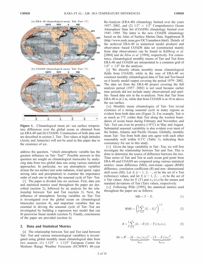
of Tair–Tsst reveals large spatial and temporal variationsover the global ocean (Figure 1), but Tsst is typicallywarmer than Tair. The magnitude of Tair–Tsst can evenbe <�3�C along the Kuroshio and Gulf Stream pathways.Because this temperature difference varies regionally, in thispaper we investigate how different atmospheric variablesaffect such changes in Tair–Tsst.[5] As expected, differences between Tair and Tsst are

closely related to processes at the air–sea interface. Atypical example is that as explained in Frankignoul[1985], net surface heat flux, in particular a combinationof latent and sensible heat fluxes involving vapor mixingratio and Tair–Tsst values, is highly correlated with Tair–Tsst, but weakly correlated with Tsst alone over most of themid–latitudes. This simply indicates that Tair–Tsst cannotbe drived from Tair or Tsst by itself, implying the existenceof other variables in its regulation.[6] Given the increasing emphasis placed on studying the

ocean’s role in climate dynamics, as mentioned above,understanding the relationship between Tair and Tsst isessential. Thus, the major objective of this paper is to

JOURNAL OF GEOPHYSICAL RESEARCH, VOL. 112, C05020, doi:10.1029/2006JC003833, 2007ClickHere

for

FullArticle

1Oceanography Division, Naval Research Laboratory, Stennis SpaceCenter, Mississippi, USA.

2Department of Statistics, University of Wisconsin, Madison,Wisconsin, USA.

Copyright 2007 by the American Geophysical Union.0148-0227/07/2006JC003833$09.00

C05020 1 of 18

http://dx.doi.org/10.1029/2006JC003833

address the question, ‘‘which atmospheric variable has thegreatest influence on Tair–Tsst?’’ Possible answers to thisquestion are sought on climatological timescales by analy-zing data from two global data sets using various statisticalapproaches. In particular, we use atmospheric variablesat/near the sea surface (net solar radiation, wind speed, vapormixing ratio and precipitation) to examine the importanceorder of each one in driving the seasonal cycle of Tair–Tsst.[7] The paper is divided into six sections. First, data sets

and statistical metrics used throughout the paper are des-cribed (section 2), followed by an analysis for the rela-tionship between Tair and Tsst (section 3). Next, theinfluence of atmospheric forcing variables on Tair–Tsstis investigated over the global ocean on climatologicaltimescales (section 4), and important variables that areessential in driving the seasonal cycle of Tair–Tsst areinvestigated by building a regression tree model that canfit piecewise linear models (section 5). Finally, conclusionsof the paper are provided (section 6).

2. Data and Statistical Metrics

[8] The relationship between Tair and Tsst (and betweenTair–Tsst and various meteorological variables) is investi-gated using global monthly mean climatological data fromtwo sources: (1) 1.125� � 1.125� European Centre forMedium–Range Weather Forecasts (ECMWF) 40-year

Re-Analysis (ERA-40) climatology formed over the years1957–2002, and (2) 1/2� � 1/2� Comprehensive OceanAtmosphere Data Set (COADS) climatology formed over1945–1989. The latter is the new COADS climatologybased on the Atlas of Surface Marine Data, Supplement B(http://www.nodc.noaa.gov/OC5/asmdnew.html). Details ofthe archived ERA-40 (a numerical model product) andobservation–based COADS data set (constructed mainlyfrom ship observations) can be found in Kallberg et al.[2004] and da Silva et al. [1994], respectively. For consis-tency, climatological monthly means of Tair and Tsst fromERA-40 and COADS are interpolated to a common grid of1.0� � 1.0� for the analyses.[9] We directly obtain monthly mean climatological

fields from COADS, while in the case of ERA-40 weconstruct monthly climatological data of Tair and Tsst basedon 6 hourly model output covering the period 1979–2002.The data set from the ERA-40 project covering the fullanalysis period (1957–2002) is not used because earliertime periods did not include many observational and satel-lite–based data sets in the re-analysis. Note that Tair fromERA-40 is at 2 m, while that from COADS is at 10 m abovethe sea surface.[10] Monthly mean climatologies of Tair–Tsst reveal

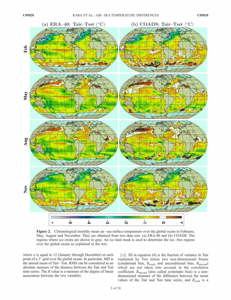
existence of a strong seasonal cycle in many regions asevident from both data sets (Figure 2). For example, Tair isas much as 5�C colder than Tsst along the western boun-daries of ocean basin during February and November, andTair–Tsst can even be positive (>0�C) in May and August.Substantial seasonal variability is also evident over most ofthe Indian, Atlantic and Pacific Oceans. Globally, monthlymean Tair–Tsst from both data sets agree with each otherreasonably well within 0.3�C (Table 1), indicating theirconsistency for use in this study.[11] Given the large variability in Tair–Tsst, we will first

investigate the relationship between Tair and Tsst. This isdone to determine the source of difference between the two.Time series of Tair and Tsst at each ocean grid point fromERA-40 and COADS are compared using various statisticalmetrics: mean difference (MD), root-mean–square (RMS)difference, correlation coefficient (R) and non–dimensionalskill score (SS). Let Xi (i = 1, 2,� � �, n) be the set of n Tsst(reference) values, and let Yi (i = 1, 2,� � �, n) be the set ofn Tair values. Also let �X (�Y ) and sX (sY) be the means andstandard deviations of Tsst (Tair) values, respectively.[12] Following Wilks [1995], the statistical metrics used

throughout the paper are as follows:

MD ¼ �Y � �X ; ð1Þ

RMS ¼ 1

n

Xni¼1

Yi � Xið Þ2 !1=2

; ð2Þ

R ¼ 1

n

Xni¼1

Xi � �Xð Þ Yi � �Yð Þ=sXsY Þ; ð3Þ

SS ¼ R2 � R� sY=sXð Þ½ 2|fflfflfflfflfflfflfflfflfflfflffl{zfflfflfflfflfflfflfflfflfflfflffl}Bcond

� �Y � �Xð Þ=sX½ 2|fflfflfflfflfflfflfflfflfflfflffl{zfflfflfflfflfflfflfflfflfflfflffl}Buncond

; ð4Þ

Figure 1. Climatological mean air–sea surface tempera-ture differences over the global ocean as obtained from(a) ERA-40 and (b) COADS. Construction of both data setsare described in section 2. Tair–Tsst values at high latitudes(Arctic and Antarctic) will not be used in this paper due tothe existence of ice.

C05020 KARA ET AL.: AIR–SEA TEMPERATURE DIFFERENCES

2 of 18

C05020

where n is equal to 12 (January through December) at eachpoint of a 1� grid over the global ocean. In particular, MD isthe annual mean of Tair–Tsst. RMS can be considered as anabsolute measure of the distance between the Tair and Tssttime series. The R value is a measure of the degree of linearassociation between the two variables.

[13] SS in equation (4) is the fraction of variance in Tairexplained by Tsst minus two non-dimensional biases(conditional bias, Bcond, and unconditional bias, Buncond)which are not taken into account in the correlationcoefficient. Buncond (also called systematic bias) is a non-dimensional measure of the difference between the meanvalues of the Tair and Tsst time series, and Bcond is a

Figure 2. Climatological monthly mean air–sea surface temperature over the global ocean in February,May, August and November. They are obtained from two data sets: (a) ERA-40 and (b) COADS. Theregions where ice exists are shown in gray. An ice land mask is used to determine the ice–free regionsover the global ocean as explained in the text.


3 of 18

C05020

measure of the relative amplitude of the variability in thetwo data sets. An examination of the SS formulationreveals that R2 is equal to SS only when Bcond and Buncond

are zero. Because these two biases are never negative,the R value can be considered to be a measure of the‘‘potential’’ skill in using Tsst to estimate Tair, i.e., theskill that one can obtain when there are no differencesbetween Tair and Tsst. A SS value of 1.0 indicates thatTair and Tsst are identical, and SS can be negative if thereis no skill between Tair and Tsst.

3. Statistical Relationship Between Tair and Tsst

[14] Comparisons between Tair and Tsst (Figure 3) areperformed using the data sets (ERA-40 and COADS) andstatistical metrics, both of which are already described insection 2. Regions where ice is present (e.g., high latitudes)are masked and shown in gray. The ice–free regions overthe global ocean are determined from an ice land mask[Reynolds et al., 2002]. The ice land mask is a function ofthe ice analysis and may change periodically. For thisreason, a climatological mean of maximum ice extent forthe mask is used in all calculations.[15] Ignoring high latitudes where sea–ice forms, the

mean difference fields are broadly similar to each otherwith Tsst warmer than Tair (generally by <1�C) nearlyeverywhere over the global ocean. Tsst is warmer becausesolar radiation is absorbed more efficiently by the ocean(and land) than by the atmosphere (i.e., troposphere isheated from below). In addition, warm Tsst relative to thesubsurface usually gives stable stratification, while thesituation is opposite for the atmosphere. Having Tsstwarmer than Tair simply explains that average sensibleheat flux is almost always cooling (warming) the ocean(atmosphere) on climatological timescales.[16] A striking feature of Figure 3 is that relatively large

Tair–Tsst values (even as large as �5�C) do exist in mid-latitudes along the western boundaries (Kuroshio and GulfStream pathways), where the RMS difference between thetwo is generally >3�C. Atmospheric advection of Tair andoceanic advection of Tsst play an important role in

determining Tair–Tsst in these regions [Yasuda et al.,2000; Qu et al., 2004; Dong and Kelly, 2004]. Overall,the results from ERA-40 and COADS are similar exceptfor differences in some regions, such as the southwesternPacific, including some regions of the Indian Ocean andhigh southern latitudes. Such discrepancies are generallyseen from maps of RMS, SS and Bcond. Not surprisingly,the discrepancies tend to occur in regions of sparseobservations especially at high latitudes.[17] There is a close relationship (large R) between Tair

and Tsst over the annual cycle in most regions (Figure 3).However, there is almost no skill between the two in threemajor regions: (i) most of the tropics, extending even tomid– latitudes in some places, (ii) along the westernboundaries, and (iii) at high southern and North Atlanticlatitudes. The low skill in all three regions is due mainlyto large differences in the mean Tair and Tsst values(i.e., large Buncond over the seasonal cycle). For COADS,Bcond and low or even negative R values play a substantialrole in giving low or negative skill in the western equato-rial Pacific warm pool and at high southern latitudes.Overall, R values are generally very high (>0.9) over mostof the global ocean. However, further analysis reveals thatwhen Tair >27�C (i.e., regions around the equator) and Tair<5�C (i.e., high southern latitudes), R values are typically<0.5, especially for COADS.[18] Based on the zonally averaged statistical metrics

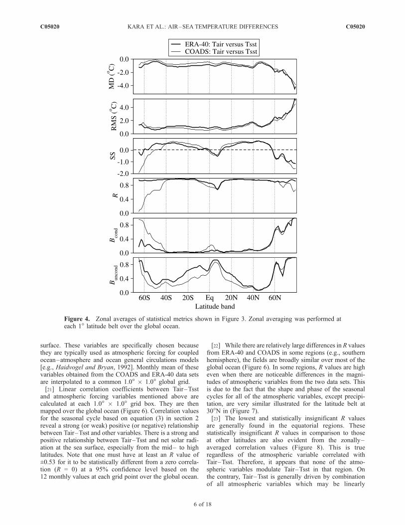
between Tair and Tsst (Figure 4), it is further confirmedthat ERA-40 and COADS give similar results over most ofthe global ocean. However, noticeable differences do showup in SS values south of 40�S. As mentioned earlier, this isdue partly to the fact that the seasonal cycle of Tair and Tsst(i.e., R) is quite different between the two data sets at thoselatitude bands. The combination of different R and Bcond

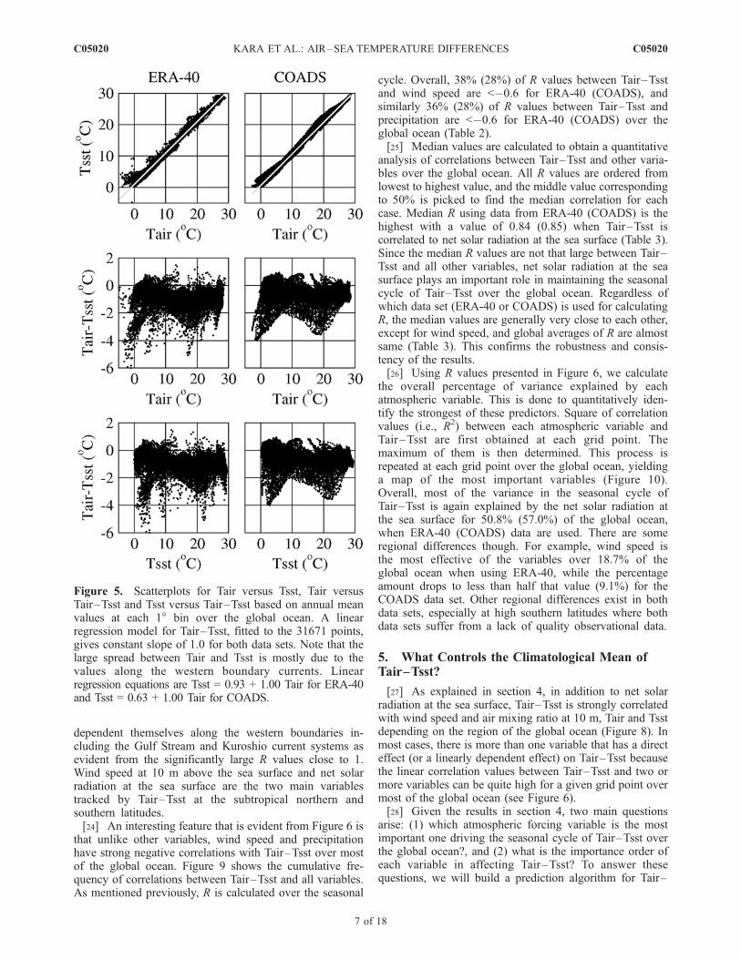
values in the two data sets results in the large differences inskill score south of 40�S.[19] We also present scatter diagrams for Tair versus

Tsst, Tair versus Tair–Tsst, and Tsst versus Tair–Tsst(Figure 5). This is done to further examine the relation-ship between Tair and Tsst and decide which one (Tair orTsst) controls Tair–Tsst. There is a strong linear relation-ship between Tair and Tsst with a R value >0.99 for bothERA-40 and COADS over the global ocean. Unlike Tairversus Tsst, there is no linear relationship between Tair(or Tsst) and Tair–Tsst (R � 0), suggesting that neitherTair nor Tsst modulates Tair–Tsst over the global ocean.This simply indicates that, as expected, there must beother factors that control Tair–Tsst, at least in someregions of the global ocean.

4. Effects of Atmospheric Variables on Tair–Tsst

[20] The results in the preceding section demonstratethat the climatological mean of Tair–Tsst must be con-trolled by variables other than Tair or Tsst itself. Thus, ourfocus here is to examine the possible effects of near–surface atmospheric variables in driving the seasonal cycleof Tair–Tsst. We consider several scalar atmosphericvariables: wind speed at 10 m above the sea surface, airmixing ratio at 10 m above the sea surface, net radiation(the total of net shortwave and net longwave radiation) atthe sea surface, Tair, Tsst and precipitation at the sea

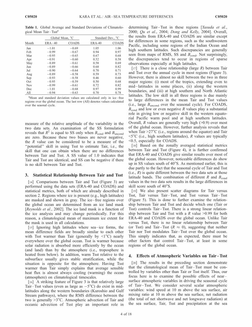
Table 1. Global Average and Standard Deviations of Climatolo-

gical Mean Tair–Tssta

Month

Global Mean, �C Standard Dev., �C

ERA–40 COADS ERA-40 COADS

Jan �1.01 �0.69 1.05 1.06Feb �0.99 �0.67 0.94 0.97Mar �0.95 �0.65 0.67 0.68Apr �0.91 �0.60 0.52 0.58May �0.89 �0.61 0.58 0.69Jun �0.89 �0.66 0.68 0.82Jul �0.90 �0.64 0.70 0.71Aug �0.89 �0.58 0.59 0.73Sep �0.93 �0.58 0.46 0.60Oct �0.95 �0.59 0.50 0.68Nov �0.99 �0.61 0.72 0.82Dec �1.01 �0.68 0.97 0.99All �0.94 �0.63 0.70 0.78aMean and standard deviation values are calculated only in ice– free

regions over the global ocean. The last row (All) denotes values calculatedover the seaonal cycle.


4 of 18

C05020

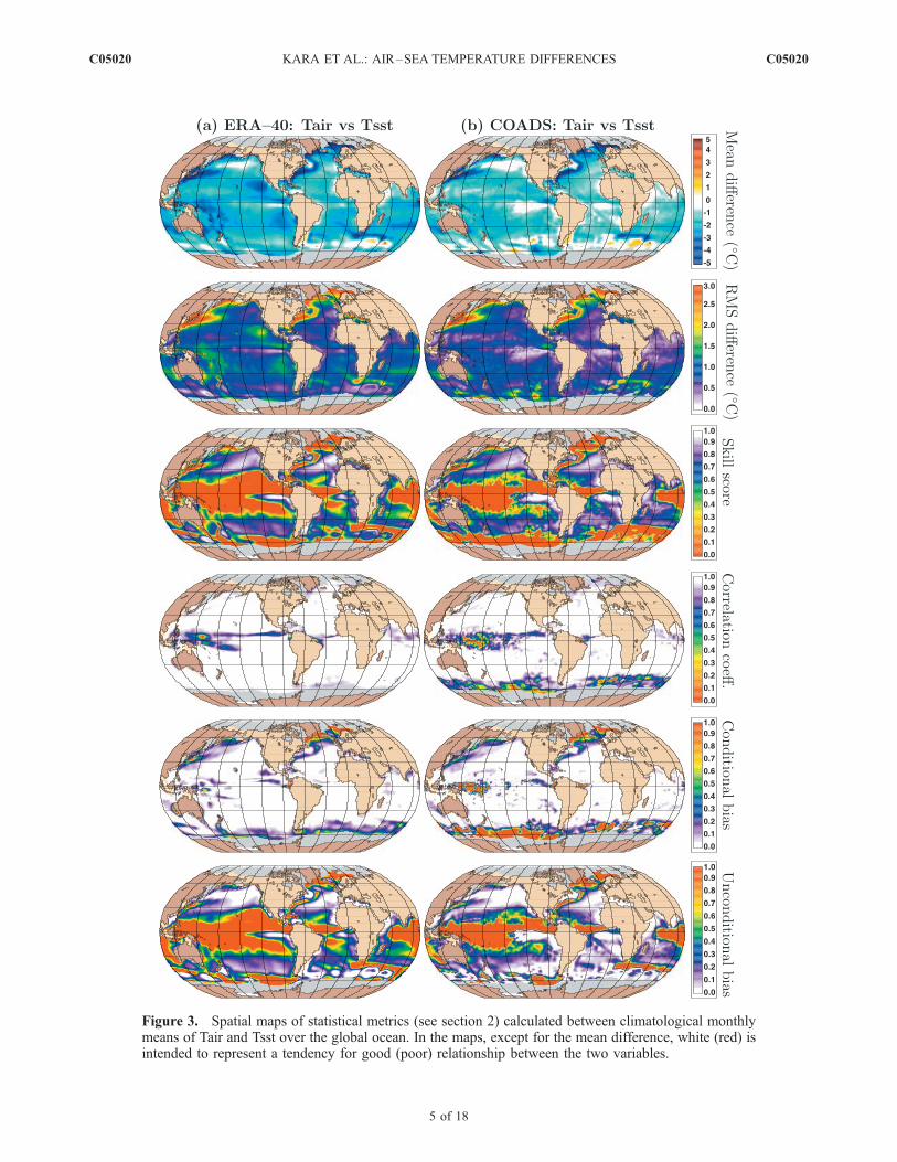
Figure 3. Spatial maps of statistical metrics (see section 2) calculated between climatological monthlymeans of Tair and Tsst over the global ocean. In the maps, except for the mean difference, white (red) isintended to represent a tendency for good (poor) relationship between the two variables.


5 of 18

C05020

surface. These variables are specifically chosen becausethey are typically used as atmospheric forcing for coupledocean–atmosphere and ocean general circulations models[e.g., Haidvogel and Bryan, 1992]. Monthly mean of thesevariables obtained from the COADS and ERA-40 data setsare interpolated to a common 1.0� � 1.0� global grid.[21] Linear correlation coefficients between Tair–Tsst

and atmospheric forcing variables mentioned above arecalculated at each 1.0� � 1.0� grid box. They are thenmapped over the global ocean (Figure 6). Correlation valuesfor the seasonal cycle based on equation (3) in section 2reveal a strong (or weak) positive (or negative) relationshipbetween Tair–Tsst and other variables. There is a strong andpositive relationship between Tair–Tsst and net solar radi-ation at the sea surface, especially from the mid– to highlatitudes. Note that one must have at least an R value of±0.53 for it to be statistically different from a zero correla-tion (R = 0) at a 95% confidence level based on the12 monthly values at each grid point over the global ocean.

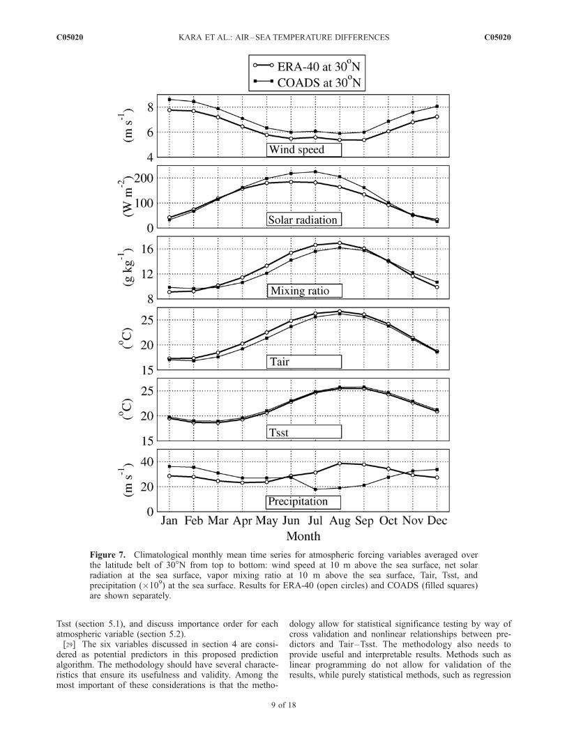
[22] While there are relatively large differences in R valuesfrom ERA-40 and COADS in some regions (e.g., southernhemisphere), the fields are broadly similar over most of theglobal ocean (Figure 6). In some regions, R values are higheven when there are noticeable differences in the magni-tudes of atmospheric variables from the two data sets. Thisis due to the fact that the shape and phase of the seasonalcycles for all of the atmospheric variables, except precipi-tation, are very similar illustrated for the latitude belt at30�N in (Figure 7).[23] The lowest and statistically insignificant R values

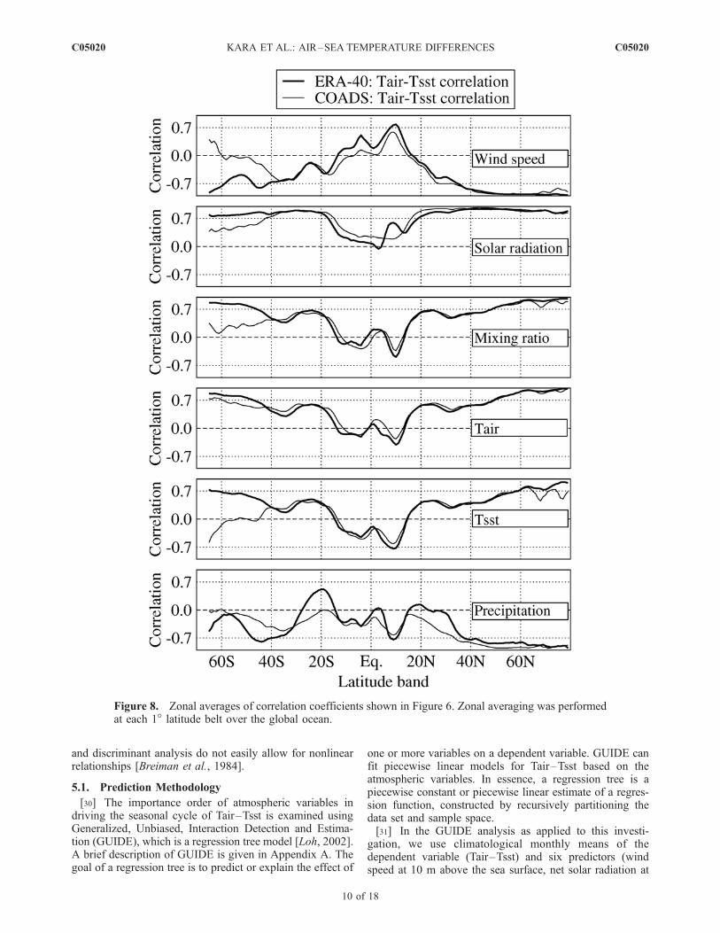
are generally found in the equatorial regions. Thesestatistically insignificant R values in comparison to thoseat other latitudes are also evident from the zonally–averaged correlation values (Figure 8). This is trueregardless of the atmospheric variable correlated withTair–Tsst. Therefore, it appears that none of the atmo-spheric variables modulate Tair–Tsst in that region. Onthe contrary, Tair–Tsst is generally driven by combinationof all atmospheric variables which may be linearly

Figure 4. Zonal averages of statistical metrics shown in Figure 3. Zonal averaging was performed ateach 1� latitude belt over the global ocean.


6 of 18

C05020

dependent themselves along the western boundaries in-cluding the Gulf Stream and Kuroshio current systems asevident from the significantly large R values close to 1.Wind speed at 10 m above the sea surface and net solarradiation at the sea surface are the two main variablestracked by Tair–Tsst at the subtropical northern andsouthern latitudes.[24] An interesting feature that is evident from Figure 6 is

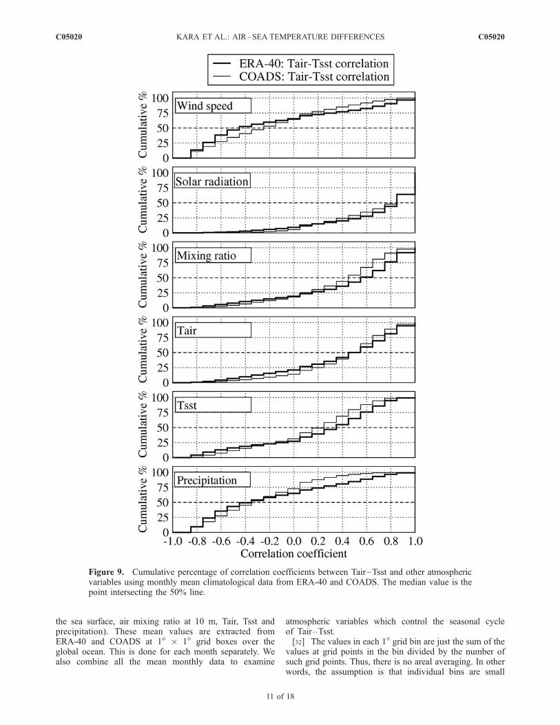
that unlike other variables, wind speed and precipitationhave strong negative correlations with Tair–Tsst over mostof the global ocean. Figure 9 shows the cumulative fre-quency of correlations between Tair–Tsst and all variables.As mentioned previously, R is calculated over the seasonal

cycle. Overall, 38% (28%) of R values between Tair–Tsstand wind speed are <�0.6 for ERA-40 (COADS), andsimilarly 36% (28%) of R values between Tair–Tsst andprecipitation are <�0.6 for ERA-40 (COADS) over theglobal ocean (Table 2).[25] Median values are calculated to obtain a quantitative

analysis of correlations between Tair–Tsst and other varia-bles over the global ocean. All R values are ordered fromlowest to highest value, and the middle value correspondingto 50% is picked to find the median correlation for eachcase. Median R using data from ERA-40 (COADS) is thehighest with a value of 0.84 (0.85) when Tair–Tsst iscorrelated to net solar radiation at the sea surface (Table 3).Since the median R values are not that large between Tair–Tsst and all other variables, net solar radiation at the seasurface plays an important role in maintaining the seasonalcycle of Tair–Tsst over the global ocean. Regardless ofwhich data set (ERA-40 or COADS) is used for calculatingR, the median values are generally very close to each other,except for wind speed, and global averages of R are almostsame (Table 3). This confirms the robustness and consis-tency of the results.[26] Using R values presented in Figure 6, we calculate

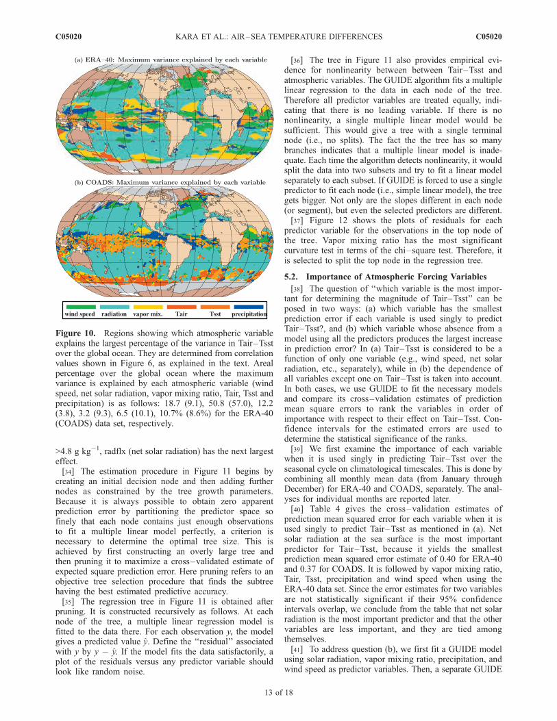
the overall percentage of variance explained by eachatmospheric variable. This is done to quantitatively iden-tify the strongest of these predictors. Square of correlationvalues (i.e., R2) between each atmospheric variable andTair–Tsst are first obtained at each grid point. Themaximum of them is then determined. This process isrepeated at each grid point over the global ocean, yieldinga map of the most important variables (Figure 10).Overall, most of the variance in the seasonal cycle ofTair–Tsst is again explained by the net solar radiation atthe sea surface for 50.8% (57.0%) of the global ocean,when ERA-40 (COADS) data are used. There are someregional differences though. For example, wind speed isthe most effective of the variables over 18.7% of theglobal ocean when using ERA-40, while the percentageamount drops to less than half that value (9.1%) for theCOADS data set. Other regional differences exist in bothdata sets, especially at high southern latitudes where bothdata sets suffer from a lack of quality observational data.

5. What Controls the Climatological Mean ofTair–Tsst?

[27] As explained in section 4, in addition to net solarradiation at the sea surface, Tair–Tsst is strongly correlatedwith wind speed and air mixing ratio at 10 m, Tair and Tsstdepending on the region of the global ocean (Figure 8). Inmost cases, there is more than one variable that has a directeffect (or a linearly dependent effect) on Tair–Tsst becausethe linear correlation values between Tair–Tsst and two ormore variables can be quite high for a given grid point overmost of the global ocean (see Figure 6).[28] Given the results in section 4, two main questions

arise: (1) which atmospheric forcing variable is the mostimportant one driving the seasonal cycle of Tair–Tsst overthe global ocean?, and (2) what is the importance order ofeach variable in affecting Tair–Tsst? To answer thesequestions, we will build a prediction algorithm for Tair–

Figure 5. Scatterplots for Tair versus Tsst, Tair versusTair–Tsst and Tsst versus Tair–Tsst based on annual meanvalues at each 1� bin over the global ocean. A linearregression model for Tair–Tsst, fitted to the 31671 points,gives constant slope of 1.0 for both data sets. Note that thelarge spread between Tair and Tsst is mostly due to thevalues along the western boundary currents. Linearregression equations are Tsst = 0.93 + 1.00 Tair for ERA-40and Tsst = 0.63 + 1.00 Tair for COADS.


7 of 18

C05020

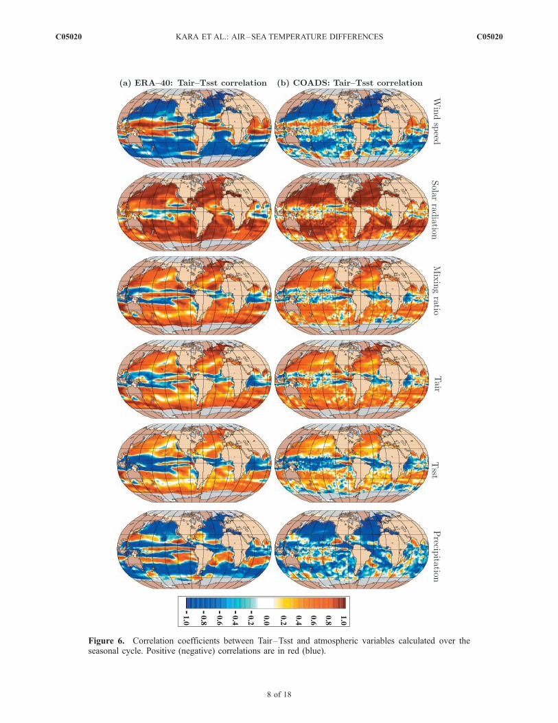
Figure 6. Correlation coefficients between Tair–Tsst and atmospheric variables calculated over theseasonal cycle. Positive (negative) correlations are in red (blue).


8 of 18

C05020

Tsst (section 5.1), and discuss importance order for eachatmospheric variable (section 5.2).[29] The six variables discussed in section 4 are consi-

dered as potential predictors in this proposed predictionalgorithm. The methodology should have several characte-ristics that ensure its usefulness and validity. Among themost important of these considerations is that the metho-

dology allow for statistical significance testing by way ofcross validation and nonlinear relationships between pre-dictors and Tair–Tsst. The methodology also needs toprovide useful and interpretable results. Methods such aslinear programming do not allow for validation of theresults, while purely statistical methods, such as regression

Figure 7. Climatological monthly mean time series for atmospheric forcing variables averaged overthe latitude belt of 30�N from top to bottom: wind speed at 10 m above the sea surface, net solarradiation at the sea surface, vapor mixing ratio at 10 m above the sea surface, Tair, Tsst, andprecipitation (�109) at the sea surface. Results for ERA-40 (open circles) and COADS (filled squares)are shown separately.


9 of 18

C05020

and discriminant analysis do not easily allow for nonlinearrelationships [Breiman et al., 1984].

5.1. Prediction Methodology

[30] The importance order of atmospheric variables indriving the seasonal cycle of Tair–Tsst is examined usingGeneralized, Unbiased, Interaction Detection and Estima-tion (GUIDE), which is a regression tree model [Loh, 2002].A brief description of GUIDE is given in Appendix A. Thegoal of a regression tree is to predict or explain the effect of

one or more variables on a dependent variable. GUIDE canfit piecewise linear models for Tair–Tsst based on theatmospheric variables. In essence, a regression tree is apiecewise constant or piecewise linear estimate of a regres-sion function, constructed by recursively partitioning thedata set and sample space.[31] In the GUIDE analysis as applied to this investi-

gation, we use climatological monthly means of thedependent variable (Tair–Tsst) and six predictors (windspeed at 10 m above the sea surface, net solar radiation at

Figure 8. Zonal averages of correlation coefficients shown in Figure 6. Zonal averaging was performedat each 1� latitude belt over the global ocean.


10 of 18

C05020

the sea surface, air mixing ratio at 10 m, Tair, Tsst andprecipitation). These mean values are extracted fromERA-40 and COADS at 1� � 1� grid boxes over theglobal ocean. This is done for each month separately. Wealso combine all the mean monthly data to examine

atmospheric variables which control the seasonal cycleof Tair–Tsst.[32] The values in each 1� grid bin are just the sum of the

values at grid points in the bin divided by the number ofsuch grid points. Thus, there is no areal averaging. In otherwords, the assumption is that individual bins are small

Figure 9. Cumulative percentage of correlation coefficients between Tair–Tsst and other atmosphericvariables using monthly mean climatological data from ERA-40 and COADS. The median value is thepoint intersecting the 50% line.


11 of 18

C05020

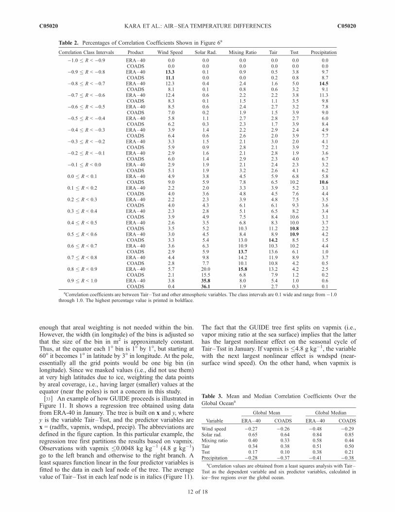
enough that areal weighting is not needed within the bin.However, the width (in longitude) of the bins is adjusted sothat the size of the bin in m2 is approximately constant.Thus, at the equator each 1� bin is 1� by 1�, but starting at60� it becomes 1� in latitude by 3� in longitude. At the pole,essentially all the grid points would be one big bin (inlongitude). Since we masked values (i.e., did not use them)at very high latitudes due to ice, weighting the data pointsby areal coverage, i.e., having larger (smaller) values at theequator (near the poles) is not a concern in this study.[33] An example of how GUIDE proceeds is illustrated in

Figure 11. It shows a regression tree obtained using datafrom ERA-40 in January. The tree is built on x and y, wherey is the variable Tair–Tsst, and the predictor variables arex = (radflx, vapmix, wndspd, precip). The abbreviations aredefined in the figure caption. In this particular example, theregression tree first partitions the results based on vapmix.Observations with vapmix 0.0048 kg kg�1 (4.8 g kg�1)go to the left branch and otherwise to the right branch. Aleast squares function linear in the four predictor variables isfitted to the data in each leaf node of the tree. The averagevalue of Tair–Tsst in each leaf node is in italics (Figure 11).

The fact that the GUIDE tree first splits on vapmix (i.e.,vapor mixing ratio at the sea surface) implies that the latterhas the largest nonlinear effect on the seasonal cycle ofTair–Tsst in January. If vapmix is 4.8 g kg�1, the variablewith the next largest nonlinear effect is wndspd (near-surface wind speed). On the other hand, when vapmix is

Table 2. Percentages of Correlation Coefficients Shown in Figure 6a

Correlation Class Intervals Product Wind Speed Solar Rad. Mixing Ratio Tair Tsst Precipitation

�1.0 R < �0.9 ERA–40 0.0 0.0 0.0 0.0 0.0 0.0COADS 0.0 0.0 0.0 0.0 0.0 0.0

�0.9 R < �0.8 ERA–40 13.3 0.1 0.9 0.5 3.8 9.7COADS 11.1 0.0 0.0 0.2 0.8 8.7

�0.8 R < �0.7 ERA–40 12.3 0.4 2.4 1.6 5.0 14.5COADS 8.1 0.1 0.8 0.6 3.2 9.1

�0.7 R < �0.6 ERA–40 12.4 0.6 2.2 2.2 3.8 11.3COADS 8.3 0.1 1.5 1.1 3.5 9.8

�0.6 R < �0.5 ERA–40 8.5 0.6 2.4 2.7 3.2 7.8COADS 7.0 0.2 1.9 1.5 3.9 9.0

�0.5 R < �0.4 ERA–40 5.8 1.1 2.7 2.8 2.7 6.0COADS 6.2 0.3 2.3 1.7 3.9 8.4

�0.4 R < �0.3 ERA–40 3.9 1.4 2.2 2.9 2.4 4.9COADS 6.4 0.6 2.6 2.0 3.9 7.7

�0.3 R < �0.2 ERA–40 3.3 1.5 2.1 3.0 2.0 4.1COADS 5.9 0.9 2.8 2.1 3.9 7.2

�0.2 R < �0.1 ERA–40 2.9 1.6 2.1 2.8 1.9 3.6COADS 6.0 1.4 2.9 2.3 4.0 6.7

�0.1 R < 0.0 ERA–40 2.9 1.9 2.1 2.4 2.3 3.2COADS 5.1 1.9 3.2 2.6 4.1 6.2

0.0 R < 0.1 ERA–40 4.9 3.8 4.5 5.9 6.8 5.8COADS 9.0 5.9 7.8 6.5 10.2 10.6

0.1 R < 0.2 ERA–40 2.2 2.0 3.3 3.9 5.2 3.1COADS 4.0 3.6 4.8 4.5 7.6 4.4

0.2 R < 0.3 ERA–40 2.2 2.3 3.9 4.8 7.5 3.5COADS 4.0 4.3 6.1 6.1 9.3 3.6

0.3 R < 0.4 ERA–40 2.3 2.8 5.1 6.5 8.2 3.4COADS 3.9 4.9 7.5 8.4 10.6 3.1

0.4 R < 0.5 ERA–40 2.6 3.5 6.8 8.3 10.0 3.7COADS 3.5 5.2 10.3 11.2 10.8 2.2

0.5 R < 0.6 ERA–40 3.0 4.5 8.4 8.9 10.9 4.2COADS 3.3 5.4 13.0 14.2 8.5 1.5

0.6 R < 0.7 ERA–40 3.6 6.3 10.9 10.3 10.2 4.4COADS 2.9 5.9 13.7 13.6 6.1 1.0

0.7 R < 0.8 ERA–40 4.4 9.8 14.2 11.9 8.9 3.7COADS 2.8 7.7 10.1 10.8 4.2 0.5

0.8 R < 0.9 ERA–40 5.7 20.0 15.8 13.2 4.2 2.5COADS 2.1 15.5 6.8 7.9 1.2 0.2

0.9 R < 1.0 ERA–40 3.8 35.8 8.0 5.4 1.0 0.6COADS 0.4 36.1 1.9 2.7 0.3 0.1

aCorrelation coefficients are between Tair–Tsst and other atmospheric variables. The class intervals are 0.1 wide and range from �1.0through 1.0. The highest percentage value is printed in boldface.

Table 3. Mean and Median Correlation Coefficients Over the

Global Oceana

Variable

Global Mean Global Median

ERA–40 COADS ERA–40 COADS

Wind speed �0.27 �0.26 �0.48 �0.29Solar rad. 0.65 0.64 0.84 0.85Mixing ratio 0.40 0.33 0.58 0.44Tair 0.34 0.38 0.51 0.50Tsst 0.17 0.10 0.38 0.21Precipitation �0.28 �0.37 �0.41 �0.38

aCorrelation values are obtained from a least squares analysis with Tair–Tsst as the dependent variable and six predictor variables, calculated inice– free regions over the global ocean.


12 of 18

C05020

>4.8 g kg�1, radflx (net solar radiation) has the next largesteffect.[34] The estimation procedure in Figure 11 begins by

creating an initial decision node and then adding furthernodes as constrained by the tree growth parameters.Because it is always possible to obtain zero apparentprediction error by partitioning the predictor space sofinely that each node contains just enough observationsto fit a multiple linear model perfectly, a criterion isnecessary to determine the optimal tree size. This isachieved by first constructing an overly large tree andthen pruning it to maximize a cross–validated estimate ofexpected square prediction error. Here pruning refers to anobjective tree selection procedure that finds the subtreehaving the best estimated predictive accuracy.[35] The regression tree in Figure 11 is obtained after

pruning. It is constructed recursively as follows. At eachnode of the tree, a multiple linear regression model isfitted to the data there. For each observation y, the modelgives a predicted value y. Define the ‘‘residual’’ associatedwith y by y � y. If the model fits the data satisfactorily, aplot of the residuals versus any predictor variable shouldlook like random noise.

[36] The tree in Figure 11 also provides empirical evi-dence for nonlinearity between between Tair–Tsst andatmospheric variables. The GUIDE algorithm fits a multiplelinear regression to the data in each node of the tree.Therefore all predictor variables are treated equally, indi-cating that there is no leading variable. If there is nononlinearity, a single multiple linear model would besufficient. This would give a tree with a single terminalnode (i.e., no splits). The fact the the tree has so manybranches indicates that a multiple linear model is inade-quate. Each time the algorithm detects nonlinearity, it wouldsplit the data into two subsets and try to fit a linear modelseparately to each subset. If GUIDE is forced to use a singlepredictor to fit each node (i.e., simple linear model), the treegets bigger. Not only are the slopes different in each node(or segment), but even the selected predictors are different.[37] Figure 12 shows the plots of residuals for each

predictor variable for the observations in the top node ofthe tree. Vapor mixing ratio has the most significantcurvature test in terms of the chi–square test. Therefore, itis selected to split the top node in the regression tree.

5.2. Importance of Atmospheric Forcing Variables

[38] The question of ‘‘which variable is the most impor-tant for determining the magnitude of Tair–Tsst’’ can beposed in two ways: (a) which variable has the smallestprediction error if each variable is used singly to predictTair–Tsst?, and (b) which variable whose absence from amodel using all the predictors produces the largest increasein prediction error? In (a) Tair–Tsst is considered to be afunction of only one variable (e.g., wind speed, net solarradiation, etc., separately), while in (b) the dependence ofall variables except one on Tair–Tsst is taken into account.In both cases, we use GUIDE to fit the necessary modelsand compare its cross–validation estimates of predictionmean square errors to rank the variables in order ofimportance with respect to their effect on Tair–Tsst. Con-fidence intervals for the estimated errors are used todetermine the statistical significance of the ranks.[39] We first examine the importance of each variable

when it is used singly in predicting Tair–Tsst over theseasonal cycle on climatological timescales. This is done bycombining all monthly mean data (from January throughDecember) for ERA-40 and COADS, separately. The anal-yses for individual months are reported later.[40] Table 4 gives the cross–validation estimates of

prediction mean squared error for each variable when it isused singly to predict Tair–Tsst as mentioned in (a). Netsolar radiation at the sea surface is the most importantpredictor for Tair–Tsst, because it yields the smallestprediction mean squared error estimate of 0.40 for ERA-40and 0.37 for COADS. It is followed by vapor mixing ratio,Tair, Tsst, precipitation and wind speed when using theERA-40 data set. Since the error estimates for two variablesare not statistically significant if their 95% confidenceintervals overlap, we conclude from the table that net solarradiation is the most important predictor and that the othervariables are less important, and they are tied amongthemselves.[41] To address question (b), we first fit a GUIDE model

using solar radiation, vapor mixing ratio, precipitation, andwind speed as predictor variables. Then, a separate GUIDE

Figure 10. Regions showing which atmospheric variableexplains the largest percentage of the variance in Tair–Tsstover the global ocean. They are determined from correlationvalues shown in Figure 6, as explained in the text. Arealpercentage over the global ocean where the maximumvariance is explained by each atmospheric variable (windspeed, net solar radiation, vapor mixing ratio, Tair, Tsst andprecipitation) is as follows: 18.7 (9.1), 50.8 (57.0), 12.2(3.8), 3.2 (9.3), 6.5 (10.1), 10.7% (8.6%) for the ERA-40(COADS) data set, respectively.


13 of 18

C05020

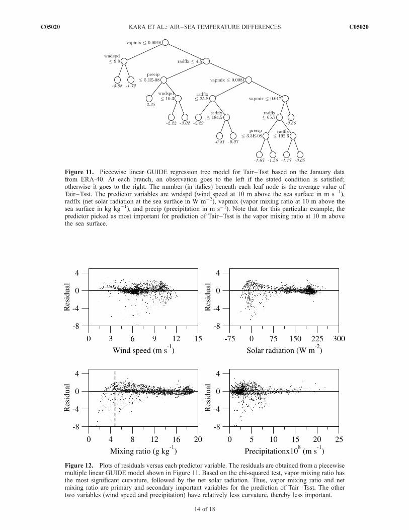
Figure 12. Plots of residuals versus each predictor variable. The residuals are obtained from a piecewisemultiple linear GUIDE model shown in Figure 11. Based on the chi-squared test, vapor mixing ratio hasthe most significant curvature, followed by the net solar radiation. Thus, vapor mixing ratio and netmixing ratio are primary and secondary important variables for the prediction of Tair–Tsst. The othertwo variables (wind speed and precipitation) have relatively less curvature, thereby less important.

Figure 11. Piecewise linear GUIDE regression tree model for Tair–Tsst based on the January datafrom ERA-40. At each branch, an observation goes to the left if the stated condition is satisfied;otherwise it goes to the right. The number (in italics) beneath each leaf node is the average value ofTair–Tsst. The predictor variables are wndspd (wind speed at 10 m above the sea surface in m s�1),radflx (net solar radiation at the sea surface in W m�2), vapmix (vapor mixing ratio at 10 m above thesea surface in kg kg�1), and precip (precipitation in m s�1). Note that for this particular example, thepredictor picked as most important for prediction of Tair–Tsst is the vapor mixing ratio at 10 m abovethe sea surface.


14 of 18

C05020

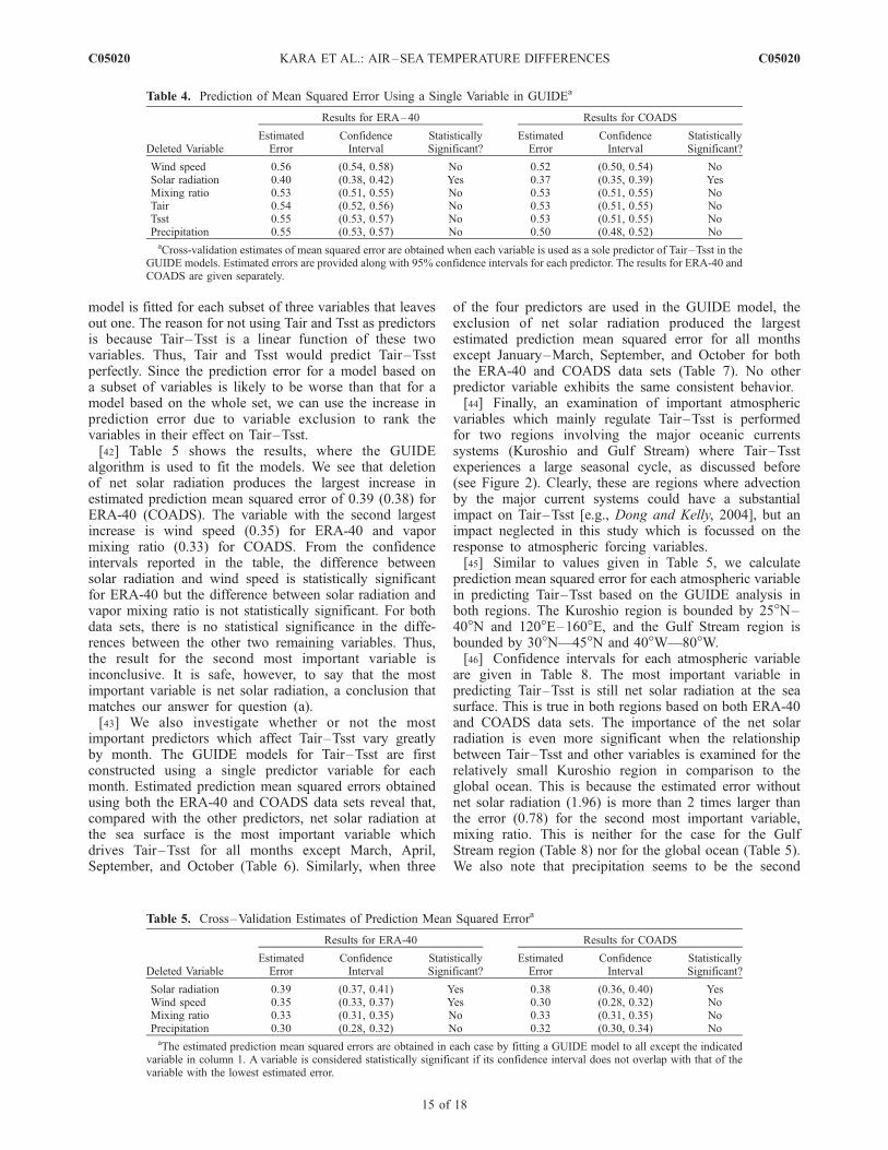
model is fitted for each subset of three variables that leavesout one. The reason for not using Tair and Tsst as predictorsis because Tair–Tsst is a linear function of these twovariables. Thus, Tair and Tsst would predict Tair–Tsstperfectly. Since the prediction error for a model based ona subset of variables is likely to be worse than that for amodel based on the whole set, we can use the increase inprediction error due to variable exclusion to rank thevariables in their effect on Tair–Tsst.[42] Table 5 shows the results, where the GUIDE

algorithm is used to fit the models. We see that deletionof net solar radiation produces the largest increase inestimated prediction mean squared error of 0.39 (0.38) forERA-40 (COADS). The variable with the second largestincrease is wind speed (0.35) for ERA-40 and vapormixing ratio (0.33) for COADS. From the confidenceintervals reported in the table, the difference betweensolar radiation and wind speed is statistically significantfor ERA-40 but the difference between solar radiation andvapor mixing ratio is not statistically significant. For bothdata sets, there is no statistical significance in the diffe-rences between the other two remaining variables. Thus,the result for the second most important variable isinconclusive. It is safe, however, to say that the mostimportant variable is net solar radiation, a conclusion thatmatches our answer for question (a).[43] We also investigate whether or not the most

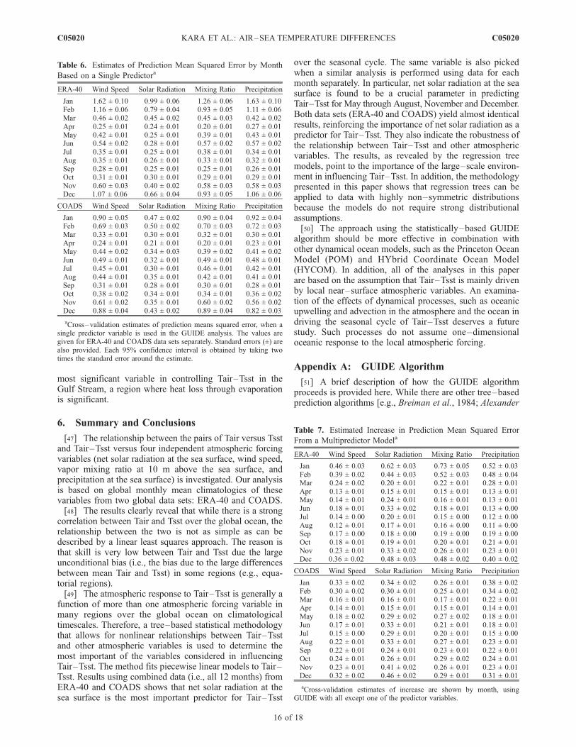
important predictors which affect Tair–Tsst vary greatlyby month. The GUIDE models for Tair–Tsst are firstconstructed using a single predictor variable for eachmonth. Estimated prediction mean squared errors obtainedusing both the ERA-40 and COADS data sets reveal that,compared with the other predictors, net solar radiation atthe sea surface is the most important variable whichdrives Tair–Tsst for all months except March, April,September, and October (Table 6). Similarly, when three

of the four predictors are used in the GUIDE model, theexclusion of net solar radiation produced the largestestimated prediction mean squared error for all monthsexcept January–March, September, and October for boththe ERA-40 and COADS data sets (Table 7). No otherpredictor variable exhibits the same consistent behavior.[44] Finally, an examination of important atmospheric

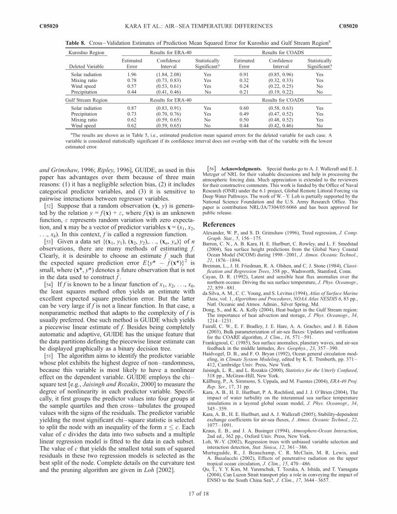
variables which mainly regulate Tair–Tsst is performedfor two regions involving the major oceanic currentssystems (Kuroshio and Gulf Stream) where Tair–Tsstexperiences a large seasonal cycle, as discussed before(see Figure 2). Clearly, these are regions where advectionby the major current systems could have a substantialimpact on Tair–Tsst [e.g., Dong and Kelly, 2004], but animpact neglected in this study which is focussed on theresponse to atmospheric forcing variables.[45] Similar to values given in Table 5, we calculate

prediction mean squared error for each atmospheric variablein predicting Tair–Tsst based on the GUIDE analysis inboth regions. The Kuroshio region is bounded by 25�N–40�N and 120�E–160�E, and the Gulf Stream region isbounded by 30�N—45�N and 40�W—80�W.[46] Confidence intervals for each atmospheric variable

are given in Table 8. The most important variable inpredicting Tair–Tsst is still net solar radiation at the seasurface. This is true in both regions based on both ERA-40and COADS data sets. The importance of the net solarradiation is even more significant when the relationshipbetween Tair–Tsst and other variables is examined for therelatively small Kuroshio region in comparison to theglobal ocean. This is because the estimated error withoutnet solar radiation (1.96) is more than 2 times larger thanthe error (0.78) for the second most important variable,mixing ratio. This is neither for the case for the GulfStream region (Table 8) nor for the global ocean (Table 5).We also note that precipitation seems to be the second

Table 4. Prediction of Mean Squared Error Using a Single Variable in GUIDEa

Deleted Variable

Results for ERA–40 Results for COADS

EstimatedError

ConfidenceInterval

StatisticallySignificant?

EstimatedError

ConfidenceInterval


Wind speed 0.56 (0.54, 0.58) No 0.52 (0.50, 0.54) NoSolar radiation 0.40 (0.38, 0.42) Yes 0.37 (0.35, 0.39) YesMixing ratio 0.53 (0.51, 0.55) No 0.53 (0.51, 0.55) NoTair 0.54 (0.52, 0.56) No 0.53 (0.51, 0.55) NoTsst 0.55 (0.53, 0.57) No 0.53 (0.51, 0.55) NoPrecipitation 0.55 (0.53, 0.57) No 0.50 (0.48, 0.52) NoaCross-validation estimates of mean squared error are obtained when each variable is used as a sole predictor of Tair–Tsst in the

GUIDE models. Estimated errors are provided along with 95% confidence intervals for each predictor. The results for ERA-40 andCOADS are given separately.

Table 5. Cross–Validation Estimates of Prediction Mean Squared Errora

Deleted Variable

Results for ERA-40 Results for COADS

EstimatedError

ConfidenceInterval


EstimatedError

ConfidenceInterval


Solar radiation 0.39 (0.37, 0.41) Yes 0.38 (0.36, 0.40) YesWind speed 0.35 (0.33, 0.37) Yes 0.30 (0.28, 0.32) NoMixing ratio 0.33 (0.31, 0.35) No 0.33 (0.31, 0.35) NoPrecipitation 0.30 (0.28, 0.32) No 0.32 (0.30, 0.34) NoaThe estimated prediction mean squared errors are obtained in each case by fitting a GUIDE model to all except the indicated

variable in column 1. A variable is considered statistically significant if its confidence interval does not overlap with that of thevariable with the lowest estimated error.


15 of 18

C05020

most significant variable in controlling Tair–Tsst in theGulf Stream, a region where heat loss through evaporationis significant.

6. Summary and Conclusions

[47] The relationship between the pairs of Tair versus Tsstand Tair–Tsst versus four independent atmospheric forcingvariables (net solar radiation at the sea surface, wind speed,vapor mixing ratio at 10 m above the sea surface, andprecipitation at the sea surface) is investigated. Our analysisis based on global monthly mean climatologies of thesevariables from two global data sets: ERA-40 and COADS.[48] The results clearly reveal that while there is a strong

correlation between Tair and Tsst over the global ocean, therelationship between the two is not as simple as can bedescribed by a linear least squares approach. The reason isthat skill is very low between Tair and Tsst due the largeunconditional bias (i.e., the bias due to the large differencesbetween mean Tair and Tsst) in some regions (e.g., equa-torial regions).[49] The atmospheric response to Tair–Tsst is generally a

function of more than one atmospheric forcing variable inmany regions over the global ocean on climatologicaltimescales. Therefore, a tree–based statistical methodologythat allows for nonlinear relationships between Tair–Tsstand other atmospheric variables is used to determine themost important of the variables considered in influencingTair–Tsst. The method fits piecewise linear models to Tair–Tsst. Results using combined data (i.e., all 12 months) fromERA-40 and COADS shows that net solar radiation at thesea surface is the most important predictor for Tair–Tsst

over the seasonal cycle. The same variable is also pickedwhen a similar analysis is performed using data for eachmonth separately. In particular, net solar radiation at the seasurface is found to be a crucial parameter in predictingTair–Tsst for May through August, November and December.Both data sets (ERA-40 and COADS) yield almost identicalresults, reinforcing the importance of net solar radiation as apredictor for Tair–Tsst. They also indicate the robustness ofthe relationship between Tair–Tsst and other atmosphericvariables. The results, as revealed by the regression treemodels, point to the importance of the large–scale environ-ment in influencing Tair–Tsst. In addition, the methodologypresented in this paper shows that regression trees can beapplied to data with highly non–symmetric distributionsbecause the models do not require strong distributionalassumptions.[50] The approach using the statistically–based GUIDE

algorithm should be more effective in combination withother dynamical ocean models, such as the Princeton OceanModel (POM) and HYbrid Coordinate Ocean Model(HYCOM). In addition, all of the analyses in this paperare based on the assumption that Tair–Tsst is mainly drivenby local near–surface atmospheric variables. An examina-tion of the effects of dynamical processes, such as oceanicupwelling and advection in the atmosphere and the ocean indriving the seasonal cycle of Tair–Tsst deserves a futurestudy. Such processes do not assume one–dimensionaloceanic response to the local atmospheric forcing.

Appendix A: GUIDE Algorithm

[51] A brief description of how the GUIDE algorithmproceeds is provided here. While there are other tree–basedprediction algorithms [e.g., Breiman et al., 1984; Alexander

Table 6. Estimates of Prediction Mean Squared Error by Month

Based on a Single Predictora

ERA-40 Wind Speed Solar Radiation Mixing Ratio Precipitation

Jan 1.62 ± 0.10 0.99 ± 0.06 1.26 ± 0.06 1.63 ± 0.10Feb 1.16 ± 0.06 0.79 ± 0.04 0.93 ± 0.05 1.11 ± 0.06Mar 0.46 ± 0.02 0.45 ± 0.02 0.45 ± 0.03 0.42 ± 0.02Apr 0.25 ± 0.01 0.24 ± 0.01 0.20 ± 0.01 0.27 ± 0.01May 0.42 ± 0.01 0.25 ± 0.01 0.39 ± 0.01 0.43 ± 0.01Jun 0.54 ± 0.02 0.28 ± 0.01 0.57 ± 0.02 0.57 ± 0.02Jul 0.35 ± 0.01 0.25 ± 0.01 0.38 ± 0.01 0.34 ± 0.01Aug 0.35 ± 0.01 0.26 ± 0.01 0.33 ± 0.01 0.32 ± 0.01Sep 0.28 ± 0.01 0.25 ± 0.01 0.25 ± 0.01 0.26 ± 0.01Oct 0.31 ± 0.01 0.30 ± 0.01 0.29 ± 0.01 0.29 ± 0.01Nov 0.60 ± 0.03 0.40 ± 0.02 0.58 ± 0.03 0.58 ± 0.03Dec 1.07 ± 0.06 0.66 ± 0.04 0.93 ± 0.05 1.06 ± 0.06

COADS Wind Speed Solar Radiation Mixing Ratio Precipitation


aCross–validation estimates of prediction means squared error, when asingle predictor variable is used in the GUIDE analysis. The values aregiven for ERA-40 and COADS data sets separately. Standard errors (±) arealso provided. Each 95% confidence interval is obtained by taking twotimes the standard error around the estimate.

Table 7. Estimated Increase in Prediction Mean Squared Error

From a Multipredictor Modela

ERA-40 Wind Speed Solar Radiation Mixing Ratio Precipitation


COADS Wind Speed Solar Radiation Mixing Ratio Precipitation


aCross-validation estimates of increase are shown by month, usingGUIDE with all except one of the predictor variables.


16 of 18

C05020

and Grimshaw, 1996; Ripley, 1996], GUIDE, as used in thispaper has advantages over them because of three mainreasons: (1) it has a negligible selection bias, (2) it includescategorical predictor variables, and (3) it is sensitive topairwise interactions between regressor variables.[52] Suppose that a random observation (x, y) is genera-

ted by the relation y = f (x) + e, where f (x) is an unknownfunction, e represents random variation with zero expecta-tion, and x may be a vector of predictor variables x = (x1, x2,. . ., xk). In this context, f is called a regression function.[53] Given a data set {(x1, y1), (x2, y2),. . ., (xn, yn)} of n

observations, there are many methods of estimating f.Clearly, it is desirable to choose an estimate f such thatthe expected square prediction error E{y* � f (x*)}2 issmall, where (x*, y*) denotes a future observation that is notin the data used to construct f .[54] If f is known to be a linear function of x1, x2, . . ., xk,

the least squares method often yields an estimate withexcellent expected square prediction error. But the lattercan be very large if f is not a linear function. In that case, anonparametric method that adapts to the complexity of f isusually preferred. One such method is GUIDE which yieldsa piecewise linear estimate of f. Besides being completelyautomatic and adaptive, GUIDE has the unique feature thatthe data partitions defining the piecewise linear estimate canbe displayed graphically as a binary decision tree.[55] The algorithm aims to identify the predictor variable

whose plot exhibits the highest degree of non–randomness,because this variable is most likely to have a nonlineareffect on the dependent variable. GUIDE employs the chi–square test [e.g., Jaisingh and Rozakis, 2000] to measure thedegree of nonlinearity in each predictor variable. Specifi-cally, it first groups the predictor values into four groups atthe sample quartiles and then cross–tabulates the groupedvalues with the signs of the residuals. The predictor variableyielding the most significant chi–square statistic is selectedto split the node with an inequality of the form x c. Eachvalue of c divides the data into two subsets and a multiplelinear regression model is fitted to the data in each subset.The value of c that yields the smallest total sum of squaredresiduals in these two regression models is selected as thebest split of the node. Complete details on the curvature testand the pruning algorithm are given in Loh [2002].

[56] Acknowledgments. Special thanks go to A. J. Wallcraft and E. J.Metzger of NRL for their valuable discussions and help in processing theatmospheric forcing data. Much appreciation is extended to the reviewersfor their constructive comments. This work is funded by the Office of NavalResearch (ONR) under the 6.1 project, Global Remote Littoral Forcing viaDeep Water Pathways. The work of W.–Y. Loh is partially supported by theNational Science Foundation and the U.S. Army Research Office. Thispaper is contribution NRL/JA/7304/05/6066 and has been approved forpublic release.

ReferencesAlexander, W. P., and S. D. Grimshaw (1996), Treed regression, J. Comp.Graph. Stat., 5, 156–175.

Barron, C. N., A. B. Kara, H. E. Hurlburt, C. Rowley, and L. F. Smedstad(2004), Sea surface height predictions from the Global Navy CoastalOcean Model (NCOM) during 1998–2001, J. Atmos. Oceanic Technol.,21, 1876–1894.

Breiman, L., J. H. Friedman, R. A. Olshen, and C. J. Stone (1984), Classi-fication and Regression Trees, 358 pp., Wadsworth, Stamford, Conn.

Cayan, D. R. (1992), Latent and sensible heat flux anomalies over thenorthern oceans: Driving the sea surface temperature, J. Phys. Oceanogr.,22, 859–881.

da Silva, A. M., C. C. Young, and S. Levitus (1994), Atlas of Surface MarineData, vol. 1, Algorithms and Procedures, NOAA Atlas NESDIS 6, 83 pp.,Natl. Oceanic and Atmos. Admin., Silver Spring, Md.

Dong, S., and K. A. Kelly (2004), Heat budget in the Gulf Stream region:The importance of heat advection and storage, J. Phys. Oceanogr., 34,1214–1231.

Fairall, C. W., E. F. Bradley, J. E. Hare, A. A. Grachev, and J. B. Edson(2003), Bulk parameterization of air-sea fluxes: Updates and verificationfor the COARE algorithm, J. Clim., 16, 571–591.

Frankignoul, C. (1985), Sea surface anomalies, planetary waves, and air-seafeedback in the middle latitudes, Rev. Geophys., 23, 357–390.

Haidvogel, D. B., and F. O. Bryan (1992), Ocean general circulation mod-eling, in Climate System Modeling, edited by K. E. Trenberth, pp. 371–412, Cambridge Univ. Press, New York.

Jaisingh, L. R., and L. Rozakis (2000), Statistics for the Utterly Confused,318 pp., McGraw-Hill, New York.

Kallberg, P., A. Simmons, S. Uppala, and M. Fuentes (2004), ERA-40 Proj.Rep. Ser., 17, 31 pp.

Kara, A. B., H. E. Hurlburt, P. A. Rochford, and J. J. O’Brien (2004), Theimpact of water turbidity on the interannual sea surface temperaturesimulations in a layered global ocean model, J. Phys. Oceanogr., 34,345–359.

Kara, A. B., H. E. Hurlburt, and A. J. Wallcraft (2005), Stability-dependentexchange coefficients for air-sea fluxes, J. Atmos. Oceanic Technol., 22,1077–1091.

Kraus, E. B., and J. A. Businger (1994), Atmosphere-Ocean Interaction,2nd ed., 362 pp., Oxford Univ. Press, New York.

Loh, W.-Y. (2002), Regression trees with unbiased variable selection andinteraction detection, Stat. Sinica, 12, 361–386.

Murtugudde, R., J. Beauchamp, C. R. McClain, M. R. Lewis, andA. Busalacchi (2002), Effects of penetrative radiation on the uppertropical ocean circulation, J. Clim., 15, 470–486.

Qu, T., Y. Y. Kim, M. Yaremchuk, T. Tozuka, A. Ishida, and T. Yamagata(2004), Can Luzon Strait transport play a role in conveying the impact ofENSO to the South China Sea?, J. Clim., 17, 3644–3657.

Table 8. Cross–Validation Estimates of Prediction Mean Squared Error for Kuroshio and Gulf Stream Regiona

Kuroshio Region Results for ERA-40 Results for COADS

Deleted VariableEstimatedError

ConfidenceInterval


EstimatedError

ConfidenceInterval


Solar radiation 1.96 (1.84, 2.08) Yes 0.91 (0.85, 0.96) YesMixing ratio 0.78 (0.73, 0.83) Yes 0.32 (0.32, 0.33) YesWind speed 0.57 (0.53, 0.61) Yes 0.24 (0.22, 0.25) NoPrecipitation 0.44 (0.41, 0.46) No 0.21 (0.19, 0.22) No

Gulf Stream Region Results for ERA-40 Results for COADS

Solar radiation 0.87 (0.83, 0.91) Yes 0.60 (0.58, 0.63) YesPrecipitation 0.73 (0.70, 0.76) Yes 0.49 (0.47, 0.52) YesMixing ratio 0.62 (0.59, 0.65) No 0.50 (0.48, 0.52) YesWind speed 0.62 (0.59, 0.65) No 0.44 (0.42, 0.46) No

aThe results are shown as in Table 5, i.e., estimated prediction mean squared errors for the deleted variable for each case. Avariable is considered statistically significant if its confidence interval does not overlap with that of the variable with the lowestestimated error.


17 of 18

C05020

Reynolds, R. W., N. A. Rayner, T. M. Smith, and D. C. Stokes (2002), Animproved in-situ and satellite SST analysis for climate, J. Clim., 15,1609–1625.

Ripley, B. D. (1996), Pattern Recognition and Neural Networks, 415 pp.,Cambridge Univ. Press, New York.

Send, U., R. C. Beardsley, and C. D. Winant (1987), Relaxation fromupwelling in the Coastal Ocean Dynamics Experiment, J. Geophys.Res., 92, 1683–1698.

Soloviev, A. V., and R. Lukas (1997), Large diurnal warming events in thenear-surface layer of the western equatorial Pacific warm pool, Deep SeaRes., 44, 1055–1076.

Soloviev, A. V., R. Lukas, and P. Hacker (2001), An approach to parame-terization of the oceanic turbulent boundary layer in the western Pacificwarm pool, J. Geophys. Res., 106, 4421–4435.

Wilks, D. S. (1995), Statistical Methods in the Atmospheric Sciences,467 pp., Elsevier, New York.

Yasuda, I., T. Tozuka, M. Noto, and S. Kouketsu (2000), Heat balance andregime shifts of the mixed layer in the Kuroshio Extension, Prog. Ocean-ogr., 47, 257–278.

Yu, L., R. A. Weller, and B. Sun (2004), Improving latent and sensible heatflux estimates for the Atlantic Ocean (1988–1999) by a synthesisapproach, J. Clim., 17, 373–393.

��H. E. Hurlburt and A. B. Kara, Oceanography Division, Naval Research

Laboratory, Code 7320, Bldg. 1009, Stennis Space Center, MS 39529,USA. ([email protected])W.-Y. Loh, Department of Statistics, University of Wisconsin, Madison,

WI 53706, USA.


18 of 18

C05020

Documents

Which near–surface atmospheric variable drives air–sea