Available online at www.sciencedirect.com

www.elsevier.com/locate/specom

Speech Communication 52 (2010) 181–200

Which words are hard to recognize? Prosodic, lexical, anddisfluency factors that increase speech recognition error rates

Sharon Goldwater a,*, Dan Jurafsky b, Christopher D. Manning c

a School of Informatics, University of Edinburgh, 10 Crichton St., Edinburgh EH8 9AB, United Kingdomb Department of Linguistics, Stanford University, Margaret Jacks Hall, Bldg. 460, Stanford, CA 94305, USA

c Department of Computer Science, Stanford University, 353 Serra Mall, Stanford, CA 94305, USA

Received 12 July 2009; received in revised form 6 October 2009; accepted 9 October 2009

Abstract

Despite years of speech recognition research, little is known about which words tend to be misrecognized and why. Previous work hasshown that errors increase for infrequent words, short words, and very loud or fast speech, but many other presumed causes of error(e.g., nearby disfluencies, turn-initial words, phonetic neighborhood density) have never been carefully tested. The reasons for the hugedifferences found in error rates between speakers also remain largely mysterious.

Using a mixed-effects regression model, we investigate these and other factors by analyzing the errors of two state-of-the-art recog-nizers on conversational speech. Words with higher error rates include those with extreme prosodic characteristics, those occurring turn-initially or as discourse markers, and doubly confusable pairs: acoustically similar words that also have similar language model proba-bilities. Words preceding disfluent interruption points (first repetition tokens and words before fragments) also have higher error rates.Finally, even after accounting for other factors, speaker differences cause enormous variance in error rates, suggesting that speaker errorrate variance is not fully explained by differences in word choice, fluency, or prosodic characteristics. We also propose that doubly con-fusable pairs, rather than high neighborhood density, may better explain phonetic neighborhood errors in human speech processing.� 2009 Elsevier B.V. All rights reserved.

Keywords: Speech recognition; Conversational; Error analysis; Individual differences; Mixed-effects model

1. Introduction

Conversational speech is one of the most difficult genresfor automatic speech recognition (ASR) systems to recog-nize, due to high levels of disfluency, non-canonical pro-nunciations, and acoustic and prosodic variability. Inorder to improve ASR performance, it is important tounderstand which of these factors is most problematic forrecognition. Previous work on recognition of spontaneousmonologues and dialogues has shown that infrequentwords are more likely to be misrecognized (Fosler-Lussierand Morgan, 1999; Shinozaki and Furui, 2001) and that

0167-6393/$ - see front matter � 2009 Elsevier B.V. All rights reserved.

doi:10.1016/j.specom.2009.10.001

* Corresponding author. Tel.: +44 131 651 5609; fax: +44 131 650 6626.E-mail addresses: sgwater@inf.ed.ac.uk (S. Goldwater), jurafsky@

stanford.edu (D. Jurafsky), manning@stanford.edu (C.D. Manning).

fast speech is associated with higher error rates (Sieglerand Stern, 1995; Fosler-Lussier and Morgan, 1999; Shino-zaki and Furui, 2001). In some studies, very slow speechhas also been found to correlate with higher error rates(Siegler and Stern, 1995; Shinozaki and Furui, 2001). InShinozaki and Furui’s (2001) analysis of a Japanese ASRsystem, word length (in phones) was found to be a usefulpredictor of error rates, with more errors on shorter words.In Hirschberg et al.’s (2004) analysis of two human–com-puter dialogue systems, misrecognized turns were foundto have (on average) higher maximum pitch and energythan correctly recognized turns. Results for speech ratewere ambiguous: faster utterances had higher error ratesin one corpus, but lower error rates in the other. Finally,Adda-Decker and Lamel (2005) demonstrated that bothFrench and English ASR systems had more trouble with

1 We describe the NIST RT-03 data set briefly below; full details,including annotation guidelines, can be found at http://www.itl.nist.gov/iad/mig/tests/rt/2003-fall/index.html.

182 S. Goldwater et al. / Speech Communication 52 (2010) 181–200

male speakers than female speakers, and suggested severalpossible explanations, including higher rates of disfluenciesand more reduction.

In parallel to these studies within the speech-recognitioncommunity, a body of work has accumulated in the psycho-linguistics literature examining factors that affect the speedand accuracy of spoken word recognition in humans.Experiments are typically carried out using isolated wordsas stimuli, and controlling for numerous factors such asword frequency, duration, and length. Like ASR systems,humans are better (faster and more accurate) at recognizingfrequent words than infrequent words (Howes, 1954; Mar-slen-Wilson, 1987; Dahan et al., 2001). In addition, it iswidely accepted that recognition is worse for words thatare phonetically similar to many other words than forhighly distinctive words (Luce and Pisoni, 1998). Ratherthan using a graded notion of phonetic similarity, psycho-linguistic experiments typically make the simplifyingassumption that two words are ‘‘similar” if they differ bya single phone (insertion, substitution, or deletion). Suchpairs are referred to as neighbors. Early on, it was shownthat both the number of neighbors of a word and the fre-quency of those neighbors are significant predictors of rec-ognition performance; it is now common to see those twofactors combined into a single predictor known as fre-

quency-weighted neighborhood density (Luce and Pisoni,1998; Vitevitch and Luce, 1999), which we discuss in moredetail in Section 3.1.

Many questions are left unanswered by these previousstudies. In the word-level analyses of Fosler-Lussier andMorgan (1999) and Shinozaki and Furui (2001), only sub-stitution and deletion errors were considered, and it isunclear whether including insertions would have led to dif-ferent results. Moreover, these studies primarily analyzedlexical, rather than prosodic, factors. Hirschberg et al.’s(2004) work suggests that utterance-level prosodic factorscan impact error rates in human–computer dialogues, butleaves open the question of which factors are important atthe word level and how they influence recognition of naturalconversational speech. Adda-Decker and Lamel’s (2005)suggestion that higher rates of disfluency are a cause ofworse recognition for male speakers presupposes that disfl-uencies raise error rates. While this assumption seems natu-ral, it was never carefully tested, and in particular neitherAdda-Decker and Lamel nor any of the other papers citedinvestigated whether disfluent words are associated witherrors in adjacent words, or are simply more likely to bemisrecognized themselves. Many factors that are oftenthought to influence error rates, such as a word’s status asa content or function word, and whether it starts a turn, alsoremained unexamined. Next, the neighborhood-related fac-tors found to be important in human word recognitionhave, to our knowledge, never even been proposed as possi-ble explanatory variables in ASR, much less formally ana-lyzed. Additionally, many of these factors are known tobe correlated. Disfluent speech, for example, is linked tochanges in both prosody and rate of speech, and low-fre-

quency words tend to have longer duration. Since previouswork has generally examined each factor independently, itis not clear which factors would still be linked to word errorafter accounting for these correlations.

A final issue not addressed by these previous studies isthat of speaker differences. While ASR error rates areknown to vary enormously between speakers (Doddingtonand Schalk, 1981; Nusbaum and Pisoni, 1987; Nusbaumet al., 1995), most previous analyses have averaged overspeakers rather than examining speaker differences explic-itly, and the causes of such differences are not well under-stood. Several early hypotheses regarding the causes ofthese differences, such as the user’s motivation to use thesystem or the variability of the user’s speech with respectto user-specific training data (Nusbaum and Pisoni,1987), can be ruled out for recognition of conversationalspeech because the user is speaking to another humanand there is no user-specific training data. However, we stilldo not know the extent to which differences in error ratesbetween speakers can be accounted for by the lexical, pro-sodic, and disfluency factors discussed above, or whetheradditional factors are at work.

The present study is designed to address the questionsraised above by analyzing the effects of a wide range of lex-ical and prosodic factors on the accuracy of two EnglishASR systems for conversational telephone speech. Weintroduce a new measure of error, individual word error rate

(IWER), that allows us to include insertion errors in ouranalysis, along with deletions and substitutions. Using thismeasure, we examine the effects of each factor on the rec-ognition performance of two different state-of-the-art con-versational telephone speech recognizers – the SRI/ICSI/UW RT-04 system (Stolcke et al., 2006) and the 2004CU-HTK system (Evermann et al., 2004b, 2005). In theremainder of the paper, we first describe the data used inour study and the individual word error rate measure.Next, we present the features we collected for each wordand the effects of those features individually on IWER.Finally, we develop a joint statistical model to examinethe effects of each feature while accounting for possible cor-relations, and to determine the relative importance ofspeaker differences other than those reflected in the featureswe collected.

2. Data

Our analysis is based on the output from two state-of-the-art speech recognition systems on the conversationaltelephone speech evaluation data from the National Insti-tute of Standards and Technology (NIST) 2003 Rich Tran-scription exercise (RT-03).1 The two recognizers are theSRI/ICSI/UW RT-04 system (Stolcke et al., 2006) andthe 2004 CU-HTK system for the DARPA/NIST RT-04

S. Goldwater et al. / Speech Communication 52 (2010) 181–200 183

evaluation (Evermann et al., 2004b, 2005).2 Our goal inchoosing these two systems, which we will refer to hence-forth as the SRI system and the Cambridge system, wasto select for state-of-the-art performance on conversationalspeech; these were two of the four best performing singleresearch systems in the world as of the NIST evaluation(Fiscus et al., 2004).

The two systems use the same architecture that is stan-dard in modern state-of-the-art conversational speech rec-ognition systems. Both systems extract Mel frequencycepstral coefficients (MFCCs) with standard normalizationand adaptation techniques: cepstral vocal tract length nor-malization (VTLN), heteroscedastic linear discriminantanalysis (HLDA), cepstral mean and variance normaliza-tion, and maximum likelihood linear regression (MLLR).Both systems have gender-dependent acoustic modelstrained discriminatively using variants of minimum phoneerror (MPE) training with maximum mutual information(MMI) priors (Povey and Woodland, 2002). Both traintheir acoustic models on approximately 2400 hours of con-versational telephone speech from the Switchboard, Call-Home and Fisher corpora, consisting of 360 hours ofspeech used in the 2003 evaluation plus 1820 hours of noisy‘‘quick transcriptions” from the Fisher corpus, althoughwith different segmentation and filtering. Both use 4-grammodels trained using in-domain telephone speech data aswell as data harvested from the web (Bulyko et al., 2003).Both use many passes or tiers of decoding, each pass pro-ducing lattices that are passed on to the next pass for fur-ther processing.

The systems differ in a number of ways. The SRI system(Stolcke et al., 2006) uses perceptual linear predictive (PLP)features in addition to MFCC features, uses novel discrim-inative phone posterior features estimated by multilayerperceptrons, and uses a variant of MPE called minimumphone frame error (MPFE). The acoustic model includesa three-way system combination (MFCC non-cross-wordtriphones, MFCC cross-word triphones, and PLP cross-word triphones). Lattices are generated using a bigram lan-guage model, and rescored with duration models, a pauselanguage model (Vergyri et al., 2002), and a syntacticallyrich SuperARV ‘almost-parsing’ language model (Wangand Harper, 2002), as well as the 4-gram models mentionedabove. The word error rate of the SRI system on the NISTRT-03 evaluation data is 18.8%.

The Cambridge system (Evermann et al., 2004b, 2005)makes use of both single-pronunciation lexicons and multi-ple-pronunciation lexicons using pronunciation probabili-ties. The acoustic model also includes a three-way systemcombination (multiple pronunciations with HLDA, multi-ple pronunciations without HLDA, and single pronuncia-

2 The SRI/ICSI/UW system was developed by researchers at SRIInternational, the International Computer Science Institute, and theUniversity of Washington. For more detailed descriptions of previous CU-HTK (Cambridge University Hidden Markov Model Toolkit) systems, seeHain et al. (2005) and Evermann et al. (2004a).

tions with HLDA). Each system uses cross-wordtriphones in a preliminary pass, then rescores with cross-word quinphone models. Whereas the SRI system uses abigram language model in the first pass, then generates lat-tices with a trigram and rescores with a 4-gram and otherlanguage models, the Cambridge system uses a trigram lan-guage model in the first pass, then generates lattices with a4-gram. The 4-gram language model includes a weightedcombination of component models, some with Kneser-Ney and some with Good-Turing smoothing, and includesthe interpolated 4-gram model used in the 2003 CU-HTKsystem (Evermann et al., 2004a). The word error rate ofthe Cambridge system on the NIST RT-03 evaluation datais 17.0%.

We examine the output of each system on the NIST RT-03 evaluation data. (Note that the developers of both theSRI and Cambridge systems had access to the evaluationdata, and so the results for both systems will be slightlybiased.) The data set contains 72 telephone conversationswith 144 speakers and 76,155 reference words. Half ofthe conversations are from the Fisher corpus and half fromthe Switchboard corpus (none from the standard portionsof these corpora used to train most ASR systems). Utter-ance breakpoint timestamps (which determine the speechsequences sent to the recognizers) were assigned by theNIST annotators. The annotation guidelines state thatbreakpoints must be placed at turn boundaries (speakerchanges), and may also be placed within turns. Forwithin-turn breakpoints, the guidelines encourage annota-tors to place these during pauses (either disfluent or atphrasal boundaries), but also permit long sequences of flu-ent speech to be broken up into smaller units for easiertranscription. Thus, in this corpus, the ‘‘utterances” beinganalyzed may comprise part or all of a turn, but do notin all cases correspond to natural breath groupings or phra-sal units.

The standard measure of error used in ASR is word error

rate (WER), computed as 100ðI þ Dþ SÞ=R, where I ; Dand S are the total number of insertions, deletions, andsubstitutions found by aligning the ASR hypotheses withthe reference transcriptions, and R is the total number ofreference words (see Fig. 1).3 However, WER can be com-puted only over full utterances or corpora. Since we wish toknow what features of a reference word increase the prob-ability of an error, we need a way to measure the errorsattributable to individual words—an individual word errorrate (IWER). We assume that a substitution or deletionerror can be assigned to its corresponding reference word(given a particular alignment), but for insertion errors,there may be two adjacent reference words that could beresponsible. Since we have no way to know which wordis responsible, we simply assign equal partial responsibility

3 Our alignments and error rates were computed using the standardNIST speech recognition evaluation script sclite, along with thenormalization (.glm) file used in the RT-03 evaluation, kindly provided byPhil Woodland.

Fig. 1. An example alignment between the reference transcription (REF) and recognizer output (HYP), with substitutions (S), deletions (D), andinsertions (I) shown. WER for this utterance is 30%.

Table 1Individual word error rates for different word types in the two systems. Final column gives the proportion of words in the data belonging to each type.Deletions of filled pauses, fragments, and guesses are not counted as errors in the standard scoring method. The total error rate for the SRI system isslightly lower than the 18.8 WER from the NIST evaluation due to the removal of the 229 insertions mentioned in Footnote 4.

SRI system Cambridge system % of data

Ins Del Sub Total Ins Del Sub Total

Full word 1.5 6.5 10.4 18.4 1.5 6.2 9.1 16.8 94.2Filled pause 0.6 – 15.4 16.1 0.9 – 15.1 16.0 2.9Fragment 2.2 – 18.8 21.1 2.0 – 18.0 20.0 1.8Backchannel 0.1 31.3 3.1 34.5 0.5 25.2 2.1 27.9 0.7Guess 2.0 – 25.3 27.3 2.5 – 26.7 29.2 0.4

Total 1.4 6.4 10.7 18.5 1.5 6.0 9.5 17.0 100

184 S. Goldwater et al. / Speech Communication 52 (2010) 181–200

for any insertion errors to both of the adjacent words. Thatis, we define IWER for the ith reference word as

IWERðwiÞ ¼ deli þ subi þ a � insi ð1Þ

where deli and subi are binary variables indicating whetherwi is deleted or substituted, and insi counts the number ofinsertions adjacent to wi. The discount factor a is chosenso that a

Pwi

insi ¼ I for the full corpus (i.e., the total pen-alty for insertion errors is the same as when computingWER). We then define IWER for a set of words as theaverage IWER for the individual words in the set:

IWERðw1 � � �wnÞ ¼1

n

Xn

i¼1

IWERðwiÞ ð2Þ

We will sometimes refer to the IWER for a set of words asthe average IWER (if necessary to distinguish from IWERfor single words), and, as is standard with WER, we willpresent it as a percentage (e.g., as 18.2 rather than .182).Note that, due to the choice of the discount factor a,IWER = WER when computed over the entire data set,facilitating direct comparisons with other studies that useWER. In this study, a ¼ :584 for the SRI system and.672 for the Cambridge system.4

The reference transcriptions used in our analysis distin-guish between five different types of words: filled pauses(um,uh), fragments (wh-, redistr-), backchannels (uh-

huh,mm-hm), guesses (where the transcribers were unsureof the correct words), and full words (everything else).Using our IWER measure, we computed error rates foreach of these types of words, as shown in Table 1. Becausemany of the features we wish to analyze can be extracted

4 Before computing a or doing any analysis, we first removed somerecognized utterances consisting entirely of insertions. These utterances allcame from a single conversation (sw_46732) in which one speaker’s turnsare (barely) audible on the other speaker’s channel, and some of theseturns were recognized by the systems. A total of 225 insertions wereremoved from the SRI output, 29 from the Cambridge output.

only for full words, and because these words constitutethe vast majority of the data, the remainder of this paperdeals only with the 71,579 in-vocabulary full words in thereference transcriptions (145 OOV full words areexcluded). Nevertheless, we note the high rate of deletionsfor backchannel words; the high rate of substitutions forfragments and guesses is less surprising.

A final point worth noting about our data set is that thereference transcriptions ordinarily used to compute WER(and here, IWER) are normalized in several ways, includ-ing treating all filled pauses as identical tokens and splittingcontractions such as it’s and can’t into individual words (itis,can not). Unless otherwise specified in Section 3.1, allfeatures we analyzed were extracted using the referencetranscriptions. A few features were extracted with the helpof a forced alignment (performed using the SRI recognizer,and kindly provided by Andreas Stolcke) between thespeech signal and a slightly different set of transcriptionsthat more accurately reflects the speakers’ true utterances.Examples of the differences between the reference tran-scriptions and the transcriptions used in the forced align-ment are shown in Table 2. We describe below how thismismatch was handled for each relevant feature.

3. Analysis of individual features

In this section, we first describe all of the features we col-lected for each word and how the features were extracted.We then provide results detailing the association betweeneach individual feature and recognition error rates.

3.1. Features

3.1.1. Disfluency features

Disfluencies are widely believed to increase ASR errorrates, but there is little published evidence to support thisbelief. In order to examine this hypothesis, and determine

Table 2Examples of differences in normalization between the reference transcrip-tions used for scoring and the transcriptions used to create a forcedalignment with the speech signal.

Reference Forced alignment

(%hesitation) in what way um in what way

o. k. okay

(%hesitation) i think it is

because

uh i think it’s

because

Fig. 2. Example illustrating disfluency features: words occurring beforeand after repetitions, filled pauses, and fragments; first, middle, and lastwords in a repeated sequence.

5 We used the parsed files rather than the tagged files because we foundthe tags to be more accurate in the parsed version. Before training thetagger, we removed punctuation and normalized hesitations. Wordstagged as foreign words, numbers, adjectives, adverbs, verbs, nouns, andsymbols were assumed to be content words; others were assumed to befunction words. In a hand-checked sample of 71 utterances, 782 out of 795full words (98.4%) were labeled with the correct broad syntactic class.

S. Goldwater et al. / Speech Communication 52 (2010) 181–200 185

whether different kinds of disfluencies have different effectson recognition, we collected several binary features indicat-ing whether each word in the data occurred before, after, oras part of a disfluency. These features are listed below andillustrated in Fig. 2.

Before/after filled pause. These features are present forwords that appear immediately preceding or followinga filled pause in the reference transcription.Before/after fragment. These features are present forwords that appear immediately preceding or followinga fragment in the reference transcription.Before/after repetition. These features are present forwords that appear immediately preceding or followinga sequence of repeated words in the reference transcrip-tion. Only identical repeated words with no interveningwords or filled pauses were considered repetitions. Whilenot all repeated words are necessarily disfluencies, wedid not distinguish between disfluent and intentionalrepetitions.

Position in repeated sequence. These additional binaryfeatures indicate whether a word is itself the first, mid-dle, or last word in a sequence of repetitions (see Fig. 2).

3.1.2. Other categorical features

Of the remaining categorical (non-numeric) features wecollected, we are aware of published results only forspeaker sex (Adda-Decker and Lamel, 2005). However,anecdotal evidence suggests that the other features maybe important in determining error rates. These features are:

Broad syntactic class. We divided words into three clas-ses: open class (e.g., nouns and verbs), closed class (e.g.,prepositions and articles), or discourse marker (e.g.,okay, well). To obtain the feature value for each word,we first tagged our data set automatically and then col-lapsed the POS tags down to the three classes used forthis feature. We used a freely available tagger (Rat-naparkhi, 1996) and trained it on the parsed portionof the Switchboard corpus in the Penn Treebank-3release (Marcus et al., 1999).5

First word of turn. To compute this feature, turn bound-aries were assigned automatically at the beginning ofany utterance following a pause of at least 100 ms dur-ing which the other speaker spoke. Preliminary analysisindicated that utterance-initial words behave similarly toturn-initial words; nevertheless, due to the possibility ofwithin-turn utterance breakpoint annotations occurringduring fluent speech (as described in Section 2), we didnot include utterance-based features.Speaker sex. This feature was extracted from the corpusmeta-data.

3.1.3. Probability features

Previous work has shown that word frequencies and/orlanguage model probabilities are an important predictor ofword error rates (Fosler-Lussier and Morgan, 1999; Shino-zaki and Furui, 2001). We used the n-gram language modelfrom the SRI system in computing our probability features(see Section 2, Bulyko et al., 2003 provides details).Because the language model was trained on transcriptionswhose normalization is closer to that of the forced align-ment than to that of the reference transcriptions, we com-puted the probability of each reference word byheuristically aligning the forced alignment transcriptionsto the reference transcriptions. For contractions listed asone word in the forced alignment and two words in the ref-

Table 3Example illustrating the preprocessing of the CMU Pronouncing Dictio-nary done before computing homophone and neighbor features. Numbersappended to phones in the original pronunciations indicate stress levels(0 = none, 1 = primary, 2 = secondary). Stress marks are removed afterdeleting extra pronunciations differing only in unstressed non-diphthongvowels and converting AH0 to AX.

Word Original pronunciation Final pronunciation

A AH0 AX

A(2) EY1 EY

ABDOMEN AE0 B D OW1 M AH0 N AE B D OW M AX N

ABDOMEN(2) AE1 B D AH0 M AH0 N AE B D AX M AX N

ABDOMINAL AE0 B D AA1 M AH0 N AH0 L AE B D AA M AX N AX L

ABDOMINAL(2) AH0 B D AA1 M AH0 N AH0 L [removed]BARGAIN B AA1 R G AH0 N [removed]BARGAIN(2) B AA1 R G IH0 N B AA R G IH N

186 S. Goldwater et al. / Speech Communication 52 (2010) 181–200

erence transcriptions (e.g., it’s versus it is), both referencewords were aligned to the same forced alignment word.6

The probability of each reference word was then deter-mined by looking up the probability of the correspondingforced alignment word in the language model. We usedtwo different probability features, listed below.

Unigram log probability. This feature is based on simpleword frequency, rather than context.Trigram log probability. This feature corresponds moreclosely to the log probabilities assigned by languagemodels in the two systems. It was computed from thelanguage model files using Katz backoff smoothing.

THE DH AH0 DH AX

THE(2) DH AH1 DH AH

THE(3) DH IY0 DH IY

3.1.4. Pronunciation-based features

The previous set of features allows us to examine therelationship between language model probabilities andword error rates; in this section we describe a set of featuresdesigned to focus on factors that might be related to acous-tic confusability. Of the features we collect here, only wordlength has been examined previously in the ASR literature,to our knowledge (Shinozaki and Furui, 2001). Most ofour pronunciation-based features are inspired by work inpsycholinguistics demonstrating that human subjects havemore difficulty recognizing spoken words that are in densephonetic neighborhoods, i.e., when there are many otherwords that differ from the target word by only a singlephone (Luce and Pisoni, 1998). In human word recognitionstudies, the effect of the number of neighbors of a word hasbeen found to be moderated by the total frequency of thoseneighbors, with high-frequency neighbors leading to slowerand less accurate recognition (Luce and Pisoni, 1998;Vitevitch and Luce, 1999). The two factors (number ofneighbors and frequency of neighbors) are often combinedinto a single measure, frequency-weighted neighborhood

density, which is generally thought to be a better predictorof recognition speed and accuracy than the raw number ofneighbors. Frequency-weighted neighborhood density iscomputed as the sum of the (log or raw) frequencies of aword’s neighbors, with frequencies computed from a largecorpus.7 It is worth noting that, unlike the words we exam-ine here, the stimuli used in studies of human word recog-nition are generally controlled for many potentialconfounds such as word length, syllable shape and number(e.g., only monosyllabic CVC words are used), intensity,

6 Due to slight differences between the two sets of transcriptions thatcould not be accounted for by normalization or other obvious changes,446 full reference words (0.6%) could not be aligned, and were excludedfrom further analysis.

7 The literature is inconsistent on the precise calculation of frequency-weighted neighborhood density, with the same authors using rawfrequencies in some cases (Luce and Pisoni, 1998) and log frequencies inothers (Luce et al., 2000; Vitevitch and Luce, 1999). Since these studiesgenerally group stimuli into only two groups (low vs. high FWND), thereis no way to determine whether log or raw frequencies are a betterpredictor. We will use log frequencies in this paper.

and speaker. In addition, stimuli are nearly always wordspresented in isolation. Thus, acoustically confusable wordscannot be disambiguated based on context. It is an openquestion whether the standard neighborhood-based psy-cholinguistic measures are important predictors of errorin ASR, where words are recognized in context.

Since we did not have access to the pronunciation dictio-naries used by the two systems in our study, we computedour pronunciation-based features using the CMU Pro-nouncing Dictionary.8 This dictionary differs from thoseordinarily used in ASR systems in distinguishing betweenseveral levels of stress, distinguishing multiple unstressedvowels (as opposed to only two, ARPABet ax and ix),and including multiple pronunciations for a large propor-tion of words. In order to bring the dictionary more in linewith standard ASR dictionaries, the following preprocess-ing steps were performed, as illustrated in Table 3. First,where two pronunciations differed only by one containinga schwa where the other contained a different unstressedshort vowel (non-diphthong), the pronunciation with theschwa was removed. Second, the unstressed central vowelAH0 was converted to AX, and all other stress marks wereremoved. After preprocessing of the dictionary, the follow-ing features were extracted.

Word length. Each word’s length in phones was deter-mined from its dictionary entry. If multiple pronuncia-tions were listed for a single word, the number ofphones in the first (longest) pronunciation was used.(Frequencies of the different pronunciations are not pro-vided in the dictionary.)Number of pronunciations. We extracted the number ofdifferent pronunciations for each word from the dictio-nary. Note that this number is not the same as the num-ber of pronunciations used in the ASR systems’

8 The CMU Pronouncing Dictionary is available from http://www.speech.cs.cmu.edu/cgi-bin/cmudict.

9 Preliminary analysis revealed that the normalized pitch values show amore systematic relationship with error rates than the unnormalizedvalues. In addition, normalizing by gender average removes the correla-tion between sex and pitch features, which is useful when building thecombined model in Section 4.

S. Goldwater et al. / Speech Communication 52 (2010) 181–200 187

dictionaries. For all but very frequent words, ASR sys-tems typically include only a single pronunciation; thisfeature may provide a better estimate of the actual pro-nunciation variability of different words.Number of homophones. We defined a homophone of thetarget word to be any word in the dictionary with a pro-nunciation identical to any of the pronunciations of thetarget word, and counted the total number of these.Number of neighbors. We computed the number ofneighbors of each word by counting the number of dis-tinct orthographic representations (other than the targetword or its homophones) whose pronunciations wereneighbors of any of the pronunciations of the targetword. For example, neighbors of the word aunt includeauntie, ain’t, and (based on the first pronunciation, ae nt), as well as want, on, and daunt (based on the secondpronunciation, ao n t).Frequency-weighted homophones/neighbors. Althoughonly frequency-weighted neighborhood density is a stan-dard measure in psycholinguistics, we also computedfrequency-weighted homophone density for complete-ness. Neighbors and homophones were determined asabove; we estimated log frequencies using the unigramlog probabilities in the SRI language model, subtractingthe smallest log probability from all values to obtainnon-negative log frequency values for all words. Thefeature values were then computed as the sum of thelog frequencies of each homophone or neighbor.

3.1.5. Prosodic features

Of the prosodic features we collected, only speech ratehas been analyzed extensively as a factor influencing worderror rates in spontaneous speech (Siegler and Stern,1995; Shinozaki and Furui, 2001; Fosler-Lussier and Mor-gan, 1999). We also extracted features based on three otherstandard acoustic–prosodic factors which could be expectedto have some effect on recognition accuracy: pitch, inten-sity, and duration. The final prosodic feature we extractedwas jitter, which is a correlate of creaky voice. Creaky voiceis becoming widespread among younger Americans, espe-cially females (Pennock-Speck et al., 2005; Ingle et al.,2005), and thus could be important to consider as a factorin recognition accuracy for these speakers.

To extract prosodic features, the transcriptions used forthe forced alignment were first aligned with the referencetranscriptions as described in the section on probabilityfeatures. The start and end time of each word in the refer-ence transcriptions could then be determined from thetimestamps in the forced alignment. For contractions listedas two reference words but one forced alignment word, anyword-level prosodic features will be identical for bothwords. The prosodic features we extracted are as follows.

Pitch. The minimum, maximum, mean, and log range ofpitch for each word were extracted using Praat(Boersma and Weenink, 2007). Minimum, maximum,

and mean values were then normalized by subtractingthe average of the mean pitch values for speakers ofthe appropriate sex, i.e., these feature values are relativeto gender norms.9 We used the log transform of thepitch range due to the highly skewed distribution of thisfeature; the transformation produced a symmetricdistribution.Intensity. The minimum, maximum, mean, and range ofintensity for each word were extracted using Praat.Speech rate. The average speech rate (in phones per sec-ond) was computed for each utterance and assigned toall words in that utterance. The number of phones wascalculated by summing the word length feature of eachword, and utterance duration was calculated using thestart and end times of the first and last words in theutterance, as given by the forced alignment. We usedthe automatically generated utterance timestamps ofthe forced alignment because the hand-annotated utter-ance boundary timestamps in the reference transcrip-tions include variable amounts of silence and non-speech noises at the beginnings and endings of utter-ances and we found the forced alignment boundariesto be more accurate.Duration. The duration of each word was extractedusing Praat.Log jitter. The jitter of each word was extracted usingPraat. Like pitch range, the distribution of jitter valuesis highly skewed; taking the log transform yields a sym-metric distribution.

Note that not all prosodic features could be extractedfrom all words in the data set. In what follows, we discussresults using three different subsets of our data: the full-word set (all 71,579 full words in the data), the prosodicset (the 67,302 full words with no missing feature values;94.0% of the full-word data set), and the no-contractionsset (the 60,618-word subset of the prosodic set obtainedby excluding all words that appear as contractions in theforced alignment transcriptions and as two separate wordsin the reference transcriptions; 84.7% of the full-word dataset).

3.2. Results and discussion

Error rates for categorical features can be found inTable 4, and error rates for numeric features are illustratedin Figs. 3 and 4. (First and middle repetitions are combinedas non-final repetitions in the table, because only 92 wordswere middle repetitions, and their error rates were similarto initial repetitions.) Despite differences in the overallerror rates between the two systems we examined, the pat-

Table 4IWER by feature for the two systems on the full-word data set. MC test

gives the proportion of samples (out of 10,000) in a Monte Carlopermutation test for which the difference between groups was at least aslarge as that observed between words with and without the given feature.% of data is the percentage of words in the data set having the givenfeature. All words is the IWER for the entire data set. (Overall IWER isslightly lower than in Table 1 due to the removal of OOV words.)

Feature SRI system Cambridge system % of data

IWER MC test IWER MC test

Before FP 16.7 .1146 15.9 .4099 1.9After FP 16.8 .2418 15.3 .1884 1.8Before frag 32.2** .0000 29.2** .0000 1.4After frag 22.0** .0008 18.5 .0836 1.4Before rep 19.6 .4508 17.0 .8666 0.7After rep 15.3* .0486 13.5* .0222 0.9Non-final rep 28.4** .0000 28.6** .0000 1.2Final rep 12.8** .0001 11.8** .0003 1.1Open-class 17.3** .0000 16.0** .0000 50.3Closed class 19.3** .0000 17.2** .0002 43.7Discourse marker 18.1 .8393 18.2* .0066 6.0Starts turn 21.0** .0000 19.5** .0000 6.2Male 19.8** .0000 18.1** .0000 49.6Female 16.7** .0000 15.3** .0000 50.4

All words 18.2 17.0 100

* Features with a significant effect on error rates according to the MonteCarlo test ðp < :05Þ.** Features with a highly significant effect on error rates according to theMonte Carlo test ðp < :005Þ.

188 S. Goldwater et al. / Speech Communication 52 (2010) 181–200

terns of errors display a striking degree of similarity. Wediscuss results for individual features in more detail below,after describing the methodology used to produce the fig-ures and significance values shown.

The error rates shown in Table 4 are based on the full-word data set, with significance levels computed using aMonte Carlo permutation test.10 For each feature, we gen-erated 10,000 random permutations of the words in thedata, and assigned the first n words in the permuted setto one group, and the remaining words to a second group(with n equal to the number of words exhibiting the givenfeature). The significance level of a given feature’s effect onerror rates can be estimated as the proportion of these sam-ples for which the difference in IWER between the twogroups is at least as large as the actual difference betweenwords that do or do not exhibit the given feature. Althoughnot shown, we computed error rates and significance levelson the prosodic and no-contractions data sets as well.Overall error rates are somewhat lower for these data sets(SRI: 18.2 full, 17.5 prosodic, 17.4 no-contractions; Cam-bridge: 16.7 full, 16.0 prosodic, 15.8 no-contractions), butthe pattern of errors is similar. For nearly all features, p-values for the smaller data sets are equal to or larger thanthose for the full data set; i.e., the smaller data sets providea more conservative estimate of significance. Consequently,

10 The permutation test is a standard nonparametric test that can be usedwith data like ours that may not conform to any particular knowndistributional form (Good, 2004).

we feel justified in basing the remaining analyses in thispaper on the smallest (no-contractions) data set, whichprovides the most accurate feature values for all words.

Figs. 3 and 4 are produced using the no-contractionsdata set. Fig. 3 includes the pronunciation-based and prob-ability features, which (with the exception of trigram prob-ability) are all lexical, in the sense that every instance of aparticular lexical item takes on the same feature value.Fig. 4 includes the prosodic features, which vary across dif-ferent instances of each lexical item. To estimate the effectsof each of these numeric features and determine whetherthey have significant predictive value for error rates, weused logistic regression (as implemented by the lrm pack-age in R). In logistic regression, the log odds of a binaryoutcome variable is modeled as a linear combination offeature values x0; . . . ; xn:

logp

1� p¼ b0x0 þ b1x1 þ � � � þ bnxn

where p is the probability that the outcome occurs andb0; . . . ; bn are coefficients (feature weights) to be estimated.If IWER were a binary variable, we could estimate the ef-fect of our features by building a separate regression modelfor each feature based on a single predictor variable – thevalue of that feature. However, IWER can take on valuesgreater than 1, so we cannot use this method. Instead, webuild a model that predicts the probability of an error(i.e., the probability that IWER is greater than zero). Thismodel will be slightly different than a model that predictsIWER itself, but for our data sets, the difference shouldbe minor: the number of words for which IWER is greaterthan one is very small (less than 1% of words in either sys-tem), so the difference between the average IWER and theprobability of an error is minimal (SRI: averageIWER = 17.4, P(error) = 17.4%; Cambridge: averageIWER = 15.8, P(error) = 15.6%). These differences arenegligible compared to the sizes of the effects of many ofthe features illustrated in Figs. 3 and 4.

While many of our numeric features exhibit a primarilylinear relationship with the log odds of an error, severalappear to have more complex patterns. To allow for thispossibility, we used restricted cubic splines to createsmooth functions of the input features.11 It is then thesefunctions that are assumed to have a linear relationshipwith the log odds. We limited the possible functions tothose with at most one inflection point (i.e., quadratic-likefunctions) and built a regression model for each feature topredict the probability of an error based on the value ofthat feature alone. The predicted values are plotted inFigs. 3 and 4 on top of the observed IWER. (Note that,although feature values were binned in order to plot theaverage observed IWER for each bin, the regression mod-els were built using the raw data.) For each feature, wedetermined whether that feature is a significant predictor

11 Restricted cubic splines were fit using the rcs function in the Designpackage (Harrell, 2007) of R (R Development Core Team, 2007).

(a) SRI system

−5 −4 −3 −2

020

40

Log probability (unigram)

IWER

|| |−6 −4 −2

020

40

Log probability (trigram)

IWER

|| |2 4 6 8 10

020

40

Word length (phones)

IWER

|| |1.0 2.0 3.0 4.0

020

40

Number of pronunciations

IWER

| |

0 2 4 6 8

020

40

Number of homophones

IWER

| |0 50 100 150 200

020

40Number of neighbors

IWER

|| |0 1 2 3 4 5 6 7

020

40

Frequency−weighted homophone

IWER

| |0 20 40 60 80 120

020

40

Frequency−weighted neighbors

IWER

|| |

(b) Cambridge system

−5 −4 −3 −2

020

40

Log probability (unigram)

IWER

|| |−6 −4 −2

020

40

Log probability (trigram)

IWER

|| |2 4 6 8 10

020

40Word length (phones)

IWER

|| |1.0 2.0 3.0 4.0

020

40

Number of pronunciations

IWER

| |

0 2 4 6 8

020

40

Number of homophones

IWER

| |0 50 100 150 200

020

40

Number of neighbors

IWER

|| |0 1 2 3 4 5 6 7

020

40

Frequency−weighted homophones

IWER

| |0 20 40 60 80 120

020

40

Frequency−weighted neighbors

IWER

|| |

Fig. 3. Effects of lexical features and trigram probability on IWER for (a) the SRI system and (b) the Cambridge system on the no-contractions data set.All feature values were binned, and the IWER for each bin is plotted, with the area of the surrounding circle proportional to the number of points in thebin. The mean value and standard deviation of each feature is provided along the bottom of each plot. Dotted lines show the IWER over the entire dataset. Solid lines show the predicted probability of an error using a logistic regression model fit to the data using the given feature as the only predictor (seetext).

S. Goldwater et al. / Speech Communication 52 (2010) 181–200 189

of errors by performing a likelihood-ratio test comparingthe model fitted using that feature as its sole predictor toa baseline model that simply fits the overall error probabil-ity in the data. All features were found to be significant pre-dictors; the slopes of the fitted probabilities in Figs. 3 and 4give a sense of the relative importance of different featuresin predicting errors.12

3.2.1. Disfluency features

Perhaps the most interesting result in Table 4 is that theeffects of disfluencies are highly variable depending on thetype of disfluency and the position of a word relative to it.Non-final repetitions and words preceding fragments havean IWER 10.2–14 points higher than the average word(e.g., words preceding fragments in the SRI system havea 32.2% IWER, 14 points above the 18.2% average), whilefinal repetitions and words following repetitions have anIWER 2.9–5.4 points lower (note, however, that the results

12 Note that, when considering only linear relationships between featurevalues and the log odds of an error, the number of neighbors and meanintensity (for both systems) and frequency-weighted neighbors (for theCambridge system) are not significant predictors of errors.

for words after repetitions are less robust – they just barelyreach the .05 significance level for the full-word SRI dataset, and do not reach significance in some of the other datasubsets). Words following fragments show a smallerincrease in errors in the SRI data set, and a non-significantincrease in the Cambridge data set. Words occurring beforerepetitions or next to filled pauses do not have significantlydifferent error rates than words in other positions. Ourresults with respect to repetitions are consistent with thework of Shriberg (1995), which suggested that only non-final repetitions are disfluencies, while the final word of arepeated sequence is fluent.

3.2.2. Other categorical features

Consistent with common wisdom, we find that open-class words have lower error rates than other words andthat words at the start of a turn have higher error rates.In addition, we find worse recognition for males than forfemales. Although some of these effects are small, theyare all statistically robust and present in both systems.The difference in recognition accuracy of 2.8–3.1% betweenmales and females is larger than the 2% found by Adda-Decker and Lamel (2005), although less than the 3.6% we

(a) SRI system

−50 0 50 100

020

40

Pitch min (Hz)

IWER

|| |−50 0 50 150

020

40

Pitch max (Hz)

IWER

|| |−50 0 50 100 150

020

40

Pitch mean (Hz)

IWER

|| |1 2 3 4 5

020

40

log(Pitch range) (Hz)

IWER

|| |

20 40 60 80

020

40

Intensity min (dB)

IWER

|| |50 60 70 80

020

40Intensity max (dB)

IWER

|| |50 60 70 80

020

40

Intensity mean (dB)

IWER

|| |10 30 50

020

40

Intensity range (dB)

IWER

|| |

5 10 15 20

020

40

Speech rate (phones/sec)

IWER

|| |0.0 0.2 0.4 0.6 0.8 1.0

020

40

Duration (sec)

IWER

|| |−6 −5 −4 −3 −2

020

40

log(Jitter)

IWER

|| |

(b) Cambridge system

−50 0 50 100

020

40

Pitch min (Hz)

IWER

|| |−50 0 50 150

020

40

Pitch max (Hz)

IWER

|| |−50 0 50 100 150

020

40

Pitch mean (Hz)

IWER

|| |1 2 3 4 5

020

40

log(Pitch range) (Hz)

IWER

|| |

20 40 60 80

020

40

Intensity min (dB)

IWER

|| |50 60 70 80

020

40

Intensity max (dB)

IWER

|| |50 60 70 80

020

40

Intensity mean (dB)

IWER

|| |10 30 50

020

40

Intensity range (dB)

IWER

|| |

5 10 15 20

020

40

Speech rate (phones/sec)

IWER

|| |0.0 0.2 0.4 0.6 0.8 1.0

020

40

Duration (sec)

IWER

|| |−6 −5 −4 −3 −2

020

40

log(Jitter)

IWER

|| |

Fig. 4. Effects of prosodic features on IWER for (a) the SRI system and (b) the Cambridge system on the no-contractions data set. Details of the plots areas in Fig. 3.

190 S. Goldwater et al. / Speech Communication 52 (2010) 181–200

found in our own preliminary work in this area (Goldwateret al., 2008), which analyzed only the SRI system and useda smaller data set.

3.2.3. Word probabilityTurning to Fig. 3, we find that low-probability words

have dramatically higher error rates than high-probabilitywords, consistent with several previous studies (Shinozakiand Furui, 2001; Fosler-Lussier and Morgan, 1999; Gold-water et al., 2008). Comparing the effects of unigram andtrigram probabilities, we see that trigram probability showsa far more linear relationship with IWER. This is not sur-prising: words that have lower language model probabili-ties can be expected to have worse recognition. Unigramprobability, while correlated with trigram probability, is a

less direct measure of the language model score, and there-fore has a more complex relationship with error.

3.2.4. Pronunciation features

While all of the pronunciation features we examined dohave a significant effect on error rates, the sizes of theeffects are in most cases fairly small. Not surprisingly,words with more possible pronunciations have higher errorrates than those with fewer, and longer words have slightlylower error rates than shorter words. The small size of theword length effect may be explained by the fact that wordlength is correlated with duration, but anti-correlated withprobability. (Table 5 shows the correlations between vari-ous features in our model.) Longer words have longerduration, which tends to decrease errors (Fig. 4), but alsolower probability, which tends to increase errors (Fig. 3).

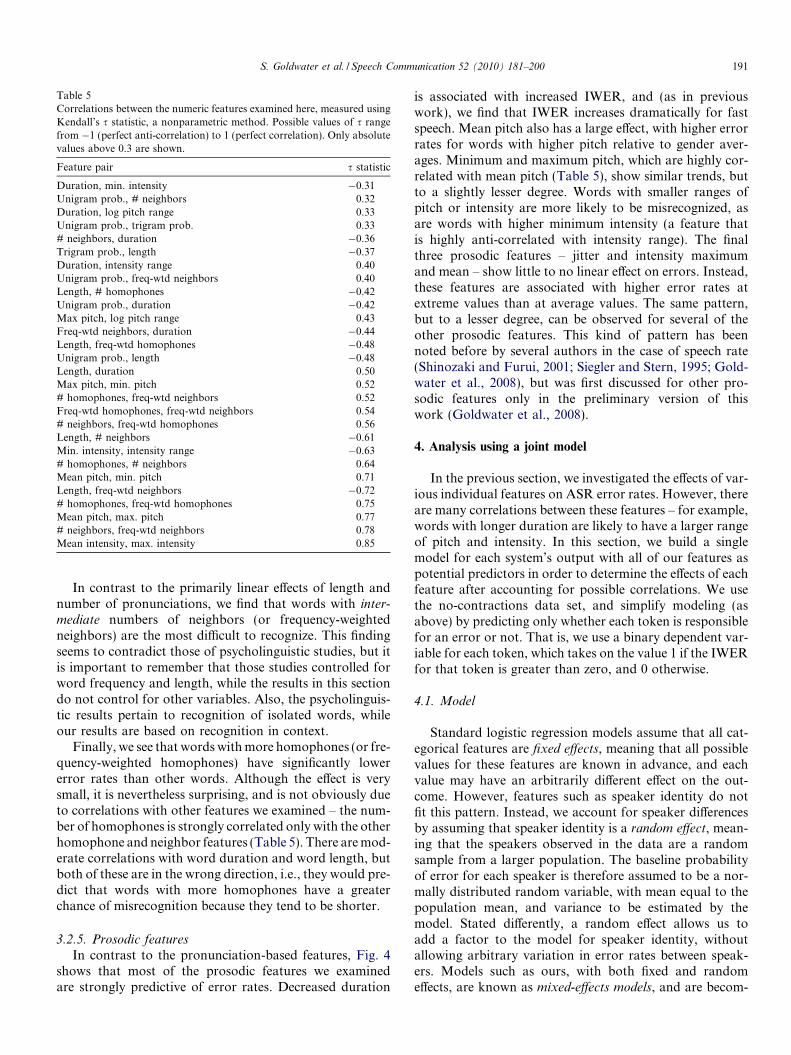
Table 5Correlations between the numeric features examined here, measured usingKendall’s s statistic, a nonparametric method. Possible values of s rangefrom �1 (perfect anti-correlation) to 1 (perfect correlation). Only absolutevalues above 0.3 are shown.

Feature pair s statistic

Duration, min. intensity �0.31Unigram prob., # neighbors 0.32Duration, log pitch range 0.33Unigram prob., trigram prob. 0.33# neighbors, duration �0.36Trigram prob., length �0.37Duration, intensity range 0.40Unigram prob., freq-wtd neighbors 0.40Length, # homophones �0.42Unigram prob., duration �0.42Max pitch, log pitch range 0.43Freq-wtd neighbors, duration �0.44Length, freq-wtd homophones �0.48Unigram prob., length �0.48Length, duration 0.50Max pitch, min. pitch 0.52# homophones, freq-wtd neighbors 0.52Freq-wtd homophones, freq-wtd neighbors 0.54# neighbors, freq-wtd homophones 0.56Length, # neighbors �0.61Min. intensity, intensity range �0.63# homophones, # neighbors 0.64Mean pitch, min. pitch 0.71Length, freq-wtd neighbors �0.72# homophones, freq-wtd homophones 0.75Mean pitch, max. pitch 0.77# neighbors, freq-wtd neighbors 0.78Mean intensity, max. intensity 0.85

S. Goldwater et al. / Speech Communication 52 (2010) 181–200 191

In contrast to the primarily linear effects of length andnumber of pronunciations, we find that words with inter-mediate numbers of neighbors (or frequency-weightedneighbors) are the most difficult to recognize. This findingseems to contradict those of psycholinguistic studies, but itis important to remember that those studies controlled forword frequency and length, while the results in this sectiondo not control for other variables. Also, the psycholinguis-tic results pertain to recognition of isolated words, whileour results are based on recognition in context.

Finally, we see that words with more homophones (or fre-quency-weighted homophones) have significantly lowererror rates than other words. Although the effect is verysmall, it is nevertheless surprising, and is not obviously dueto correlations with other features we examined – the num-ber of homophones is strongly correlated only with the otherhomophone and neighbor features (Table 5). There are mod-erate correlations with word duration and word length, butboth of these are in the wrong direction, i.e., they would pre-dict that words with more homophones have a greaterchance of misrecognition because they tend to be shorter.

3.2.5. Prosodic features

In contrast to the pronunciation-based features, Fig. 4shows that most of the prosodic features we examinedare strongly predictive of error rates. Decreased duration

is associated with increased IWER, and (as in previouswork), we find that IWER increases dramatically for fastspeech. Mean pitch also has a large effect, with higher errorrates for words with higher pitch relative to gender aver-ages. Minimum and maximum pitch, which are highly cor-related with mean pitch (Table 5), show similar trends, butto a slightly lesser degree. Words with smaller ranges ofpitch or intensity are more likely to be misrecognized, asare words with higher minimum intensity (a feature thatis highly anti-correlated with intensity range). The finalthree prosodic features – jitter and intensity maximumand mean – show little to no linear effect on errors. Instead,these features are associated with higher error rates atextreme values than at average values. The same pattern,but to a lesser degree, can be observed for several of theother prosodic features. This kind of pattern has beennoted before by several authors in the case of speech rate(Shinozaki and Furui, 2001; Siegler and Stern, 1995; Gold-water et al., 2008), but was first discussed for other pro-sodic features only in the preliminary version of thiswork (Goldwater et al., 2008).

4. Analysis using a joint model

In the previous section, we investigated the effects of var-ious individual features on ASR error rates. However, thereare many correlations between these features – for example,words with longer duration are likely to have a larger rangeof pitch and intensity. In this section, we build a singlemodel for each system’s output with all of our features aspotential predictors in order to determine the effects of eachfeature after accounting for possible correlations. We usethe no-contractions data set, and simplify modeling (asabove) by predicting only whether each token is responsiblefor an error or not. That is, we use a binary dependent var-iable for each token, which takes on the value 1 if the IWERfor that token is greater than zero, and 0 otherwise.

4.1. Model

Standard logistic regression models assume that all cat-egorical features are fixed effects, meaning that all possiblevalues for these features are known in advance, and eachvalue may have an arbitrarily different effect on the out-come. However, features such as speaker identity do notfit this pattern. Instead, we account for speaker differencesby assuming that speaker identity is a random effect, mean-ing that the speakers observed in the data are a randomsample from a larger population. The baseline probabilityof error for each speaker is therefore assumed to be a nor-mally distributed random variable, with mean equal to thepopulation mean, and variance to be estimated by themodel. Stated differently, a random effect allows us toadd a factor to the model for speaker identity, withoutallowing arbitrary variation in error rates between speak-ers. Models such as ours, with both fixed and randomeffects, are known as mixed-effects models, and are becom-

Table 6Summary of features used in the unreduced joint model, showing whether each feature is a F(ixed) or R(andom) effect, whether it is B(inary), N(umeric),or C(ategorical), and the associated degrees of freedom (d.f.). Numeric features were fit using restricted cubic splines with two degrees of freedom, exceptfor NUM-PRONUNCIATIONS, which does not take on enough different values to fit a non-linear spline.

Feature F/R Type d.f. Feature F/R Type d.f.

BEFORE-FP F B 1 UNIGRAM-PROB F N 2AFTER-FP F B 1 TRIGRAM-PROB F N 2BEFORE-FRAG F B 1 WORD-LENGTH F N 2AFTER-FRAG F B 1 NUM-PRONUNCIATIONS F N 1BEFORE-REP F B 1 NUM-HOMOPHONES F N 2AFTER-REP F B 1 FREQ-WTD-NEIGHBORS F N 2FINAL-REP F B 1 PITCH-MEAN F N 2NON-FINAL-REP F B 1 LOG-PITCH-RANGE F N 2OPEN-CLASS F B 1 INTENSITY-MEAN F N 2DISCOURSE-CLASS F B 1 INTENSITY-RANGE F N 2STARTS-TURN F B 1 SPEECH-RATE F N 2SEX F B 1 DURATION F N 2CORPUS F B 1 JITTER F N 2CELLULAR-LINE F B 1 SPEAKER-ID R C 1LAND-LINE F B 1 WORD-ID R C 1CORDLESS-LINE F B 1

(a) SRI system

−1.5 −1.0 −0.5 0.0 0.5 1.0 1.5

corpus=SWsex=Mstarts turnbefore FPbefore fragbefore repnon−final repopen class

(b) Cambridge system

−1.5 −1.0 −0.5 0.0 0.5 1.0 1.5

corpus=SWis cellularstarts turnbefore FPbefore fragafter repnon−final repdiscourse marker

Fig. 5. Estimates and standard errors of the coefficients for the categorical features found to be significant predictors in the reduced model for each system.

192 S. Goldwater et al. / Speech Communication 52 (2010) 181–200

ing a standard method for analyzing linguistic data (Baa-yen, 2008). We fit our models using the lme4 package(Bates, 2007) of R (R Development Core Team, 2007).

To analyze the joint effects of all of our features, we ini-tially built as large a model as possible, and used backwards

elimination to remove features one at a time whose presencedid not contribute significantly (at p < :05) to model fit.The predictors in our initial model are summarized inTable 6. They included all of the features described above,with the exception of number of neighbors, frequency-weighted homophones, pitch minimum and maximum,and intensity minimum and maximum. These features wereexcluded because of high correlations with other features inthe model, which makes parameter estimation in the com-bined model difficult. All categorical features (those inTable 4) were converted to binary variables, and additionalbinary features were added to account for corpus (Fisher orSwitchboard) and telephone line type (standard, cellular,cordless, land). All numeric features (those in Figs. 3 and4) were rescaled to values between 0 and 1 in order to makethe model coefficients for different features comparable,13

and then centered to ensure a mean value of 0.

13 Before rescaling, 39 data points with outlying feature values wereremoved: two words with speech rate above 27 phones per second, 13words with duration above 1.25 s, and 24 words with log jitter below �7.

To account for the possibility that some of the numericfeatures in our model have non-linear effects (as suggestedby our analysis in Section 3), our initial model includedfunctions of these features with at most one inflectionpoint, again modeled using the restricted cubic splines(rcs) function in R. (The backwards elimination processcan be used to eliminate the extra parameters associatedwith the non-linear components of each predictor as neces-sary.) In addition, we included random effects for speakeridentity and word identity. Thus, the initial model includes44 degrees of freedom: 43 for the features shown in Table 6,and one for the intercept.

4.2. Results and discussion

Fig. 5 shows the estimated coefficients and standarderrors for each of the fixed effect categorical featuresremaining in the reduced model (i.e., after backwards elim-ination). Since all of the features are binary, a coefficient ofb indicates that the corresponding feature, when present,adds a weight of b to the log odds (i.e., multiplies the oddsof an error by a factor of eb). Thus, features with positivecoefficients increase the odds of an error, and features withnegative coefficients decrease the odds of an error. Themagnitude of the coefficient corresponds to the size of theeffect.

S. Goldwater et al. / Speech Communication 52 (2010) 181–200 193

The coefficients for our numeric features are not directlyinterpretable in most cases, since they are computed interms of the orthogonal basis functions of the restrictedcubic splines used to fit the non-linear components of themodel. However, the coefficients can be used to plot thepredicted effect of each feature on the log odds of an error,yielding the visualization in Fig. 6. Positive y values indi-cate increased odds of an error, and negative y values indi-cate decreased odds of an error. The x axes in these plotsreflect the rescaled and centered values of each feature, sothat all x axes are one unit long, with the mean observedvalue of each feature always equal to zero.

4.2.1. Disfluencies

In our analysis of individual features, we found that dif-ferent types of disfluencies have different effects: non-finalrepeated words and words before fragments have highererror rates, while final repetitions and words following rep-

(a) SRI system

−0.2 0.2 0.6

−40

24

Pitch mean

log

odds

|| |−0.4 0.0 0.4

−40

24

Log pitch range

log

odds

|| |

log

odds

−0.4 0.0 0.4

−40

24

Speech rate

log

odds

|| |−0.2 0.2 0.6

−40

24

Duration

log

odds

|| |

log

odds

−0.6 −0.2 0.2

−40

24

Trigram log prob

log

odds

|| |−0.6 −0.2 0.2

−40

24

Unigram log prob

log

odds

|| |

log

odds

(b) Cambridge system

−0.2 0.2 0.6

−40

24

Pitch mean

log

odds

|| |−0.4 0.0 0.4

−40

24

Log pitch range

log

odds

|| |

log

odds

−0.4 0.0 0.4

−40

24

Speech rate

log

odds

|| |−0.2 0.2 0.6

−40

24

Duration

log

odds

|| |

log

odds

−0.6 −0.2 0.2

−40

24

Trigram log prob

log

odds

|| |−0.6 −0.2 0.2

−40

24

Unigram log prob

log

odds

|| |

log

odds

Fig. 6. Predicted effect of each numeric feature on the log odds of an error. Onsystem are shown. The mean value and standard deviation of each feature (afterrescaling, all x axes are one unit long; the range of values shown reflects the r

etitions have lower error rates. After accounting for corre-lations between factors, a slightly different picture emerges.Non-final repeated words and words before fragments stillhave the greatest chance of an error, but there is no longera beneficial effect for final repetitions, and the effect forwords after repetitions is only found in the Cambridge sys-tem. Both systems now show increased chances of error forwords before filled pauses, and words before repetitions arealso associated with more errors in the SRI system. Over-all, disfluencies tend to have a negative effect on recogni-tion, increasing the odds of an error by as much as afactor of 3.7.

Many of the differences in disfluency patterns from Sec-tion 3 (specifically, the reduction or elimination of theapparent beneficial effect of final repetitions and words fol-lowing repetitions, and the appearance of a negative effectbefore filled pauses) may be explained as follows. Wordsnear filled pauses and repetitions have longer duration than

−0.6 −0.2 0.2

−40

24

Intensity mean

|| |−0.2 0.2 0.6

−40

24

Intensity range

log

odds

|| |

−0.4 0.0 0.4

−40

24

Log jitter

|| |0.0 0.4 0.8

−40

24

Word length

log

odds

|| |

−0.4 0.0 0.4

−40

24

Freq−wtd neighbors

|| |

−0.6 −0.2 0.2

−40

24

Intensity mean

|| |−0.2 0.2 0.6

−40

24

Intensity range

log

odds

|| |

−0.4 0.0 0.4

−40

24

Log jitter

|| |0.0 0.4 0.8

−40

24

Word length

log

odds

|| |

−0.4 0.0 0.4

−40

24

Freq−wtd neighbors

|| |0.0 0.4 0.8

−40

24

No. pronunciations

log

odds

| |

ly features found to be significant predictors in the reduced model for eachrescaling and centering) is provided along the bottom of each plot. Due to

ange of values observed in the data.

194 S. Goldwater et al. / Speech Communication 52 (2010) 181–200

other words (Bell et al., 2003), and longer duration lowersIWER. Taking duration into account therefore reduces anyapparent positive effects of disfluencies, and reveals previ-ously obscured negative effects. Also, according to Shriberg(1995), the vast majority of repetitions are so-called ‘‘retro-spective” repetitions (Heike, 1981), in which the initialword(s) are disfluent, but the final word resumes fluentspeech. Our results fit nicely with this hypothesis, since finalrepetitions have no significant effect in our combinedmodel, while non-final repetitions incur a penalty.

4.2.2. Other categorical features

Without including in the model other lexical or prosodicfeatures, we found that a word is more likely to be misrec-ognized at the beginning of a turn, and less likely to be mis-recognized if it is an open-class word. According to ourjoint model, the start-of-turn effect still holds even afteraccounting for the effects of other features. This suggeststhat contextual (i.e., language modeling) factors are notthe explanation for the start-of-turn effect; articulatorystrengthening is a possible alternative (Fougeron and Keat-ing, 1997; Keating et al., 2003). The open-class effectappears in our joint model for the SRI system, althoughin the Cambridge system open-class words do not seemto have a beneficial effect; instead, discourse markers arefound to have a negative effect. As in the individual model,all of these effects are fairly small.

As for speaker sex, we find that male speakers no longerhave significantly higher error rates than females in theCambridge system. Males do have significantly highererror rates than females in the SRI system, but the differ-ence is small (a factor of 1.2 in the odds), and the signifi-cance level is now only .04, as compared to below .0001in the individual analysis. These results shed some lighton the work of Adda-Decker and Lamel (2005), who sug-gested several factors that could explain males’ higher errorrates. In particular, they showed that males have higherrates of disfluency, produce words with slightly shorterdurations, and use more alternate (‘‘sloppy”) pronuncia-tions. Our joint model incorporates the first two of thesefactors, and by doing so greatly reduces the difference inerror rates between males and females. This suggests thatdisfluency and duration indeed account for much of the dif-ference in recognition accuracy. The remaining small differ-ences may be accounted for by males’ increased use ofalternate pronunciations, as suggested by Adda-Deckerand Lamel (2005). Another possibility is that female speechis more easily recognized because females tend to haveexpanded vowel spaces (Diehl et al., 1996), a factor thatis associated with greater intelligibility (Bradlow et al.,1996) and is characteristic of genres with lower ASR errorrates (Nakamura et al., 2008).

4.2.3. Word probability

Not surprisingly, we find that even after accounting forthe effects of correlated features, word probability still hasa very strong effect on recognition performance, with

higher error rates for low-probability words. Interestingly,both unigram and trigram probabilities have strong inde-pendent effects, with the trigram language model probabil-ity being the more influential. It is also worth noting thatthe non-linear trends appearing in the individual analysiswere not found to be significant in the combined model,except for a small but significant effect ðp < :025Þ in theCambridge unigram probability. Thus, our modelingresults suggest that a word’s frequency and its languagemodel probability are both independently related to thechance of its being recognized correctly in a near linearway.

4.2.4. Pronunciation features

Our combined model considered four pronunciation-based features: word length, number of pronunciations,number of homophones, and frequency-weighted neigh-bors. Only two of these were found to be significant predic-tors in both systems: word length (with longer wordshaving lower error rates) and frequency-weighted neigh-bors (with intermediate values having higher error rates).The effect of word length is greater than in the individualanalysis, which supports our hypothesis that correlationswith duration and probability obscured the word lengtheffect in that analysis. We have no explanation at this timefor the non-linear effect of frequency-weighted neighbors,which persists despite our model’s incorporation of otherfactors such as word frequency and length.

Number of pronunciations was found to be a significantpredictor only in the Cambridge system, where words withmore pronunciations had higher error rates.

4.2.5. Prosodic features

Examining the effects of pitch and intensity individually,we found that increased range for these features is associ-ated with lower IWER, while higher pitch and extremesof intensity are associated with higher IWER. In the jointmodel, we now see that means of pitch and intensity areactually stable over a wide range of the most common val-ues, but errors increase for extreme values of pitch (on thehigh end) and intensity (on the low end). A greater range ofintensity is still associated with lower error rates despiteaccounting for the effects of duration, which one mightexpect to be the cause of this trend in the individual anal-ysis. However, the benefit of greater pitch range is nolonger seen; instead, extreme values of pitch range on eitherend seem to be problematic (although the effect is small).

In the individual analysis, both speech rate and durationwere strongly tied to error rates. While both of these fea-tures are still important in the combined model, durationis shown to have by far the greater effect of the two. Unlikemost of the other prosodic features we examined, includingspeech rate, average values of duration do not have thelowest error rates. Rather, above-average duration is asso-ciated with the lowest error rates. For words with extre-mely long duration, recognition begins to degrade again.Note that, although one might expect speech rate and dura-

S. Goldwater et al. / Speech Communication 52 (2010) 181–200 195

tion to be highly correlated, we found a relatively low cor-relation of s ¼ �0:15. Only a small part of the variability induration can be explained by speech rate; the rest is due tovariations in word length and other factors.

For our final prosodic feature, log jitter, we found in theindividual analysis that extreme values were associatedwith higher error rates. This finding was replicated in thecombined model.

Overall, the results from our joint analysis suggest that,other things being equal, recognition performance is bestfor words with typical values of most prosodic features(duration being the notable exception), and degrades asfeature values become more extreme.

4.2.6. Differences between lexical items

As discussed above, our models contain a random effectfor word identity, to account for the possibility that certainlexical items have higher error rates that are not explainedby any of the other factors in the model. It is worth askingwhether this random effect is really necessary. To addressthis question, we compared the fit to each system’s dataof two different models: our initial full model containingall of our fixed effects (including both linear and non-linearterms) and random effects for both speaker identity andword identity, and a similar model containing all the samefeatures except for word identity. Results are shown inTable 7. For both systems, the fit of the model without arandom effect for word identity is significantly worse than

Table 7Fit to the data of various models and their degrees of freedom (d.f.). Full mosignificantly to fit; Baseline contains only intercept. Other models are obtainedsyntactic class, start-of-turn), all probability features (unigram and trigram pfrequency-weighted neighbors, number of pronunciations), all prosodic featuidentity, or the random effect for word identity. Diff is the difference in log likepairwise comparisons except Full vs. Reduced, as computed using a likelihood

Model SRI

Neg. log lik. Diff.

Full 24,305 0Reduced 24,316 11Baseline 28,006 3701No categorical 24,475 159No probability 24,981 664No pronunciation 24,347 31No prosodic 25,150 834No speaker 25,069 753No word 24,627 322

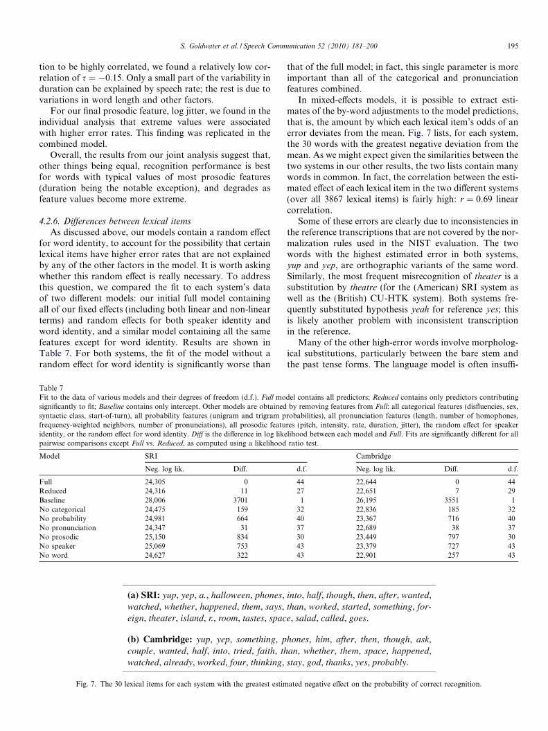
Fig. 7. The 30 lexical items for each system with the greatest estim

that of the full model; in fact, this single parameter is moreimportant than all of the categorical and pronunciationfeatures combined.

In mixed-effects models, it is possible to extract esti-mates of the by-word adjustments to the model predictions,that is, the amount by which each lexical item’s odds of anerror deviates from the mean. Fig. 7 lists, for each system,the 30 words with the greatest negative deviation from themean. As we might expect given the similarities between thetwo systems in our other results, the two lists contain manywords in common. In fact, the correlation between the esti-mated effect of each lexical item in the two different systems(over all 3867 lexical items) is fairly high: r ¼ 0:69 linearcorrelation.

Some of these errors are clearly due to inconsistencies inthe reference transcriptions that are not covered by the nor-malization rules used in the NIST evaluation. The twowords with the highest estimated error in both systems,yup and yep, are orthographic variants of the same word.Similarly, the most frequent misrecognition of theater is asubstitution by theatre (for the (American) SRI system aswell as the (British) CU-HTK system). Both systems fre-quently substituted hypothesis yeah for reference yes; thisis likely another problem with inconsistent transcriptionin the reference.

Many of the other high-error words involve morpholog-ical substitutions, particularly between the bare stem andthe past tense forms. The language model is often insuffi-

del contains all predictors; Reduced contains only predictors contributingby removing features from Full: all categorical features (disfluencies, sex,

robabilities), all pronunciation features (length, number of homophones,res (pitch, intensity, rate, duration, jitter), the random effect for speakerlihood between each model and Full. Fits are significantly different for allratio test.

Cambridge

d.f. Neg. log lik. Diff. d.f.

44 22,644 0 4427 22,651 7 291 26,195 3551 1

32 22,836 185 3240 23,367 716 4037 22,689 38 3730 23,449 797 3043 23,379 727 4343 22,901 257 43

ated negative effect on the probability of correct recognition.

0 10 20 30 40 50 60

010

2030

4050

60

IWER, SRI

IWER

, Cam

brid

ge

Fig. 8. A comparison of speaker error rates in the two systems. Each pointrepresents a single speaker.

196 S. Goldwater et al. / Speech Communication 52 (2010) 181–200

cient to distinguish these two forms, since they can occurwith similar neighboring words (e.g., they watch them andthey watched them are both grammatical and sensible),and they are also similar acoustically. Examples of thiskind of error, with their most frequent substitution inparentheses, include the following reference words: called(call), asked (ask), asks (asked), happened (happen), says

(said), started (start), thinking (think), tried (try), wanted

(want), watched (watch), tastes (taste), phones (phone), andgoes (go).

In addition to these morphological substitutions, severalother high-error words are also frequently substituted withhomophones or near-homophones that can occur in similarcontexts, in particular than (and), then (and), him (them),and them (him). The high error rates found for these wordsmay explain why we did not find strong effects for neigh-borhood density overall. In most situations, the contextin which a word is spoken is sufficient to disambiguatebetween acoustically similar candidates, so competitionfrom phonetically neighboring words is not usually a prob-lem. Errors in ASR are caused not by words with largenumbers of similar neighbors, but by words with one ortwo strong competitors that can occur in similar contexts.Put another way, acoustically confusable words are nottypically a problem, but doubly confusable pairs—wordpairs with similar language model scores in addition to sim-ilar acoustic scores—can be a source of errors. This findingalso suggests that the effects of neighborhood density inhuman word recognition might also be significantlyreduced when words are recognized in context rather thanin isolation, as is typical in experimental settings.

Finally, we note that the words in the previous para-graph (than, then, him, and them) are very frequentlydeleted as well as being substituted. This is probably dueto a combination of lack of disambiguating context (e.g.,would want him to be and would want to be are both accept-able, and then and and mean essentially the same thing) andthe fact that these words are subject to massively reducedpronunciations, often due to cliticization (him and them

are generally cliticized to the preceding verb; then is oftencliticized to the following word). Other words with higherror that are known to be subject to massive reductioninclude something, already, and probably suggesting thatall these examples may be due to pronunciation factorsbeyond those captured by simple duration.

4.2.7. Differences between speakersAs we have already mentioned, ASR error rates are

known to differ greatly between speakers. Using themixed-effects logistic regression methodology presentedhere, it is possible to examine the extent to which these dif-ferences can be explained by variation in speakers’ patternsof lexical choice, prosody, or disfluency. We first used thesame method described above to analyze the overall impor-tance of the random effect for speaker identity in our fittedmodels. As shown in Table 7, removing the random effectfor speaker identity from the full models results in a much

worse fit to the data. That is, the lexical, prosodic, and dis-fluency variables examined here are not sufficient to fullyexplain the differences in error rates between speakers. Infact, the speaker effect is the single most important factorin the models for both the SRI and Cambridge data sets,and is more important than any other feature group asidefrom the prosodic features. Note that, as with the otherfeatures we analyzed, the error rates of different speakersare similar in the two data sets, with a linear correlationof .92. Fig. 8 illustrates. Thus, whichever factors areresponsible for the speaker-specific differences in recogni-tion, they seem to behave similarly with respect to both sys-tems, unlike some of the speaker differences found in thework of Nusbaum and Pisoni (1987) with much earliersystems.

In addition to analyzing the overall importance ofspeaker identity in our models, we can also examine theestimated effects of individual speakers, just as we did forindividual words in the previous section. Fig. 9 shows theby-speaker adjustments to the model predictions, with theactual probability of error for each speaker given for refer-ence. Notice that the estimated adjustments do not com-pletely track speaker error rates, as they would if speakeridentity were the only factor in the model. This indicatesthat the other factors in our model do explain some ofthe variation in error rates between speakers, just not all.

At this point, it seems natural to ask whether differentspeakers might not only have different overall error rates,but different patterns of errors – that is, does changingthe values of certain features affect error rates differentlyfor different speakers? The models presented here assumethat each speaker has a different baseline error rate, butthat the effects of each feature are the same for eachspeaker. Using techniques similar to those used here, itwould theoretically be possible to introduce additional ran-dom effects for the intercepts (or even slopes) of each fea-ture on a speaker-by-speaker basis, and to test for thesignificance of these additional parameters. However, thenumber of possible models for comparison would be enor-mous, so a purely exploratory analysis (similar to our own)

(a) SRI system

P(er

ror)

010

3050

log

odds

−1.5

−0.5

0.5

1.5

(b) Cambridge system

P(er

ror)

010

3050

log

odds

−1.5

−0.5

0.5

1.5

Fig. 9. Empirical probability of a recognition error for each speaker (top) and estimated change in the log odds of an error for each speaker (bottom).Each bar corresponds to a single speaker, with both graphs for a single system sorted according to the speakers’ error probability under that system.

30 50 70 90

0.0

0.2

0.4

Intensity mean (dB)

Fitte

d P(

err)

−100 0 100 200

0.0

0.2

0.4

Pitch mean (Hz)0.0 0.5 1.0 1.5

0.0

0.2

0.4

Duration (sec)−8 −6 −4 −2 0

0.0

0.2

0.4

Log prob (trigram)0 10 20 30

0.0

0.2

0.4

Speech rate (ph/sec)

30 50 70 90

0.0

0.2

0.4

Intensity mean (dB)

Fitte

d P(

err)

−100 0 100 200

0.0

0.2

0.4

Pitch mean (Hz)0.0 0.5 1.0 1.5

0.0

0.2

0.4

Duration (sec)−8 −6 −4 −2 0

0.0

0.2

0.4

Log prob (trigram)0 10 20 30

0.0

0.2

0.4

Speech rate (ph/sec)

Fig. 10. Estimated effects of various features on the error rates of two different speakers (top: speaker fsh_60682_b, bottom: speaker sw_47282_b) usingthe SRI system. Dashed lines illustrate the baseline probability of error for each speaker. Solid lines were obtained by fitting a logistic regression model toeach speaker’s data, with the variable labeled on the x-axis as the only predictor.

S. Goldwater et al. / Speech Communication 52 (2010) 181–200 197

is infeasible at present. To our knowledge, there are cur-rently no automated model selection tools for mixed-effectsmodels with multiple random effects, so analysis involves ahuman in the loop. Moreover, the complexity of our cur-rent models already pushes the boundary of what can bedone with reasonable time and accuracy using the numeri-cal optimization procedures that are available to fit themodels.14 Nevertheless, it is possible to get some sense ofthe variability between speakers by fitting separate logisticregression models to each speaker’s data and plotting theresults. Fig. 10 illustrates some of the differences betweentwo speakers chosen fairly arbitrarily from our data set,showing that the estimated effects of various features arequite different for the two speakers. For example, the esti-mated error rate increases dramatically for speakerfsh_60682_b as mean pitch increases, while speaker

14 Our largest model takes about an hour to fit on a 2.66 GHzworkstation. Introducing more random effects would increase this timesignificantly, and could create problems with the accuracy of the finalmodel fit as well.

sw_47282_b shows almost no effect of pitch. Similar kindsof variability appear in the rest of the data set in both sys-tems and for many of the features we examined. Althoughwe do not know whether these differences are statisticallysignificant, they are certainly suggestive that the effects ofmany features may vary considerably between speakers.

Since our models assume that features behave similarlyacross speakers, this suggestion might cause some readersto question the validity of our analysis and conclusions.However, we emphasize that the trends we have foundare still an accurate reflection of the average behavior ofthe systems across a number of speakers. Statistical analy-ses of complex data sets have always been limited by theavailable technology, and we can only hope to incremen-tally improve our understanding of the phenomena in ques-tion by making use of the best tools available at the time.The mixed-effects models used here are a step up from pre-vious work in which speaker differences were not modeledat all, and even correlations between features were oftenignored. As new statistical modeling tools become avail-able, we may be able to further refine our understanding

198 S. Goldwater et al. / Speech Communication 52 (2010) 181–200

of speaker differences. However, it is already clear that,despite the speaker adaptation models used in the systemswe analyzed, speaker differences remain an importantsource of error in ASR and an important challenge forfuture research.

5. Conclusion

In this paper, we introduced the individual word error

rate (IWER) for measuring ASR performance on individ-ual words, including insertions as well as deletions and sub-stitutions. Using IWER, we analyzed the effects of a largevariety of lexical, disfluency, contextual, and prosodic fea-tures in two different ASR systems, both individually andin a joint model. We found that despite differences in theoverall performance of the two systems, the effects of thefactors we examined were extremely similar. In particular,our analysis revealed the following effects. (1) Words at thestart of a turn have slightly higher IWER than average, andopen-class (content) words have slightly lower IWER.However, only the former effect persists in both systemsafter accounting for the effects of other factors. (2) Disflu-encies heavily impact error rates: IWER for non-final rep-etitions and words preceding fragments rises by up to 14%absolute, while IWER for final repetitions and words fol-lowing repetitions decreases by up to 5.4% absolute. Afteraccounting for the effect of prosodic features, the latterbenefit is nearly eliminated, and a negative effect for wordsbefore filled pauses is revealed, suggesting that the effects ofthese disfluencies are normally obscured by the greaterduration of nearby words. (3) For most acoustic–prosodicfeatures (including pitch mean and range, intensity mean,jitter, and speech rate) there is little effect on recognitionperformance over a range of typical values, but errorsincrease for words with more extreme values in one or bothdirections (other factors being equal). The exception isduration, for which higher-than-average values yield thebest performance. (4) After accounting for the effects ofother factors, both unigram and trigram probability havestrong independent effects on error rates, with the oddsof an error increasing nearly linearly as probabilitydecreases. (5) The probability of misrecognizing a word isonly very weakly correlated with the number of neighborsof that word (similar-sounding words), and is uncorrelatedwith the number of homophones (identical-soundingwords). However, these factors seem to be more importantwhen contextual cues (language model probabilities) areinsufficient to disambiguate similar-sounding words. (6)Although the factors we examined can account for someof the variance in error rates between speakers, unex-plained differences between speakers are still a major factorin determining word error rates.

Our results have a number of implications for automaticspeech recognition. The first concerns the role of disfluen-cies. About 15% of the words in our conversational tele-phone speech corpora are either disfluencies or adjacentto disfluencies, underscoring the importance of understand-

ing how disfluencies contribute to error rates. We find thatin fact, only some types of disfluencies are problematic—specifically, fragments, non-final repetitions, and wordspreceding fragments. These kinds of words constituteabout 4% of our corpora, but nevertheless cause a signifi-cant number of errors due to their hugely inflated errorrates. Taken together, these results highlight the impor-tance of continued research on disfluencies for decreasingrecognition error rates in spontaneous speech, and alsoprovide a guide as to which types of disfluencies might bemore profitable to study.

Similarly, the fact that extreme prosodic values led tomore errors, as well as the large individual differences wefound, suggests that our current systems are not doing agood job of adapting to prosodic variation within andamong speakers. Current algorithms for speaker-adaptivetraining such as MLLR and VTLN, focused as they areon cepstral values, are capable only of adjusting forspeaker differences in segmental (phone) realization. Whileprosodic factors in speech processing have traditionallybeen studied in the context of speech synthesis rather thanspeech recognition, augmenting speaker-adaptive trainingto deal with prosodic variation may require explicit repre-sentation of prosodic aspects of the speech signal inrecognition.

Our results suggest not only that speaker variation is animportant remaining source of errors, but also provide atleast a first step toward refining the search for the possiblelocus of this variation. Even after accounting for prosodicfactors like pitch, intensity, and rate of speech, as well aslanguage model, pronunciation, and disfluency factors,we found speaker differences to have a large role in deter-mining error rates. This shows that none of the other basicfactors we examined is the crucial source of speaker differ-ences affecting recognition errors. Better understanding ofspeaker differences must remain a major direction forfuture research.

Finally, our analysis of the random effect for word iden-tity suggests a new important factor that increases errorwhen a word is a member of a doubly confusable pair: a pairof similar-sounding words that can also occur in very sim-ilar contexts. Such pairs include morphological substitu-tions between bare stem and past tense (preterite) formslike ask/asked, says/said, watch/watched and want/wanted,or pairs that are homophones when reduced, like than/and and him/them. Because examples like they ask himand they asked him are acoustically similar and similarlygrammatical, neither the acoustic model nor the languagemodel has sufficient evidence to distinguish them.

One way to improve discrimination of these pairs in rec-ognition might be to build sets of binary classifiers that aredesigned to disambiguate exactly these situations when runas a rescoring procedure on lattice or confusion networkoutput. For example, a him/them classifier might be ableto make use of sophisticated natural language features,such as coreferring singular or plural nouns that occur else-where in the discourse. A stem/preterite classifier could

S. Goldwater et al. / Speech Communication 52 (2010) 181–200 199

make use of adverbial or other hints about tense or aspectin the clause.

Our results on these lexical effects may also have impli-cations for the study of human speech recognition. As wementioned above, one of the most replicated studies inhuman speech recognition shows that humans subjectshave difficulty recognizing similar-sounding words (Luceand Pisoni, 1998; Vitevitch and Luce, 1999). This resulthas been modeled by proposing that recognition of a targetword is affected by the number and frequency of similar-sounding words, the frequency-weighted neighborhooddensity. But previous studies of human word recognitiongenerally consist of isolated words. Our findings suggestthe possibility that such difficulties may disappear whenwords are presented in context. In most situations, the con-text in which a word is spoken is sufficient to disambiguatebetween acoustically similar candidates, and indeed we sawthat for ASR, competition from phonetically neighboringwords is not usually a problem. Instead, we suggest thatdifficulties in human word recognition in context arecaused not by words with large numbers of similar neigh-bors, but by doubly confusable pairs, i.e., homophonesor neighbors with similar contextual predictability. Thefact that our error analysis of automatic speech recognitionhelped us to develop a hypotheses about human speech rec-ognition highlights the importance of the joint study ofhuman and machine language processing.

Acknowledgments

This work was supported by the Edinburgh–StanfordLINK and ONR MURI award N000140510388. We thankAndreas Stolcke for providing the SRI recognizer output,language model, and forced alignments; Phil Woodlandfor providing the Cambridge recognizer output and otherevaluation data; and Katrin Kirchhoff and RaghunandanKumaran for datasets used in preliminary work, usefulscripts, and additional help.

References

Adda-Decker, M., Lamel, L., 2005. Do speech recognizers prefer femalespeakers? In: Proc. INTERSPEECH, pp. 2205–2208.

Baayen, R.H., 2008. Analyzing Linguistic Data. In: A Practical Intro-duction to Statistics. Cambridge University Press, Cambridge, UK.

Bates, D., 2007. lme4: Linear mixed-effects models using S4 classes. Rpackage version 0.99875-8.

Bell, A., Jurafsky, D., Fosler-Lussier, E., Girand, C., Gregory, M., Gildea,D., 2003. Effects of disfluencies, predictability, and utterance positionon word form variation in English conversation. J. Acoust. Soc. Amer.113 (2), 1001–1024.

Boersma, P., Weenink, D., 2007. Praat: doing phonetics by computer(version 4.5.16). Available from <http://www.praat.org/>.

Bradlow, A., Torretta, G., Pisoni, D., 1996. Intelligibility of normalspeech I: Global and fine-grained acoustic–phonetic talker character-istics. Speech Comm. 20, 255–272.

Bulyko, I., Ostendorf, M., Stolcke, A., 2003. Getting more mileage fromweb text sources for conversational speech language modeling usingclass-dependent mixtures. In: Proc. Conf. on Human LanguageTechnologies.

Dahan, D., Magnuson, J., Tanenhaus, M., 2001. Time course of frequencyeffects in spoken-word recognition: evidence from eye movements.Cognit. Psychol. 42, 317–367.

Diehl, R., Lindblom, B., Hoemeke, K., Fahey, R., 1996. On explainingcertain male–female differences in the phonetic realization of vowelcategories. J. Phonetics 24, 187–208.

Doddington, G., Schalk, T., 1981. Speech recognition: turning theory topractice. IEEE Spectrum 18, 26–32.

Evermann, G., Chan, H.Y., Gales, M.J.F., Hain, T., Liu, X., Wang, L.,Mrva, D., Woodland, P.C., 2004a. Development of the 2003 CU-HTKconversational telephone speech transcription system. In: Proc.ICASSP.

Evermann, G., Chan, H.Y., Gales, M.J.F., Jia, B., Liu, X., Mrva, D., Sim,K.C., Wang, L., Woodland, P.C., Yu, K., 2004b. Development of the2004 CU-HTK English CTS systems using more than two thousandhours of data. In: Proc. Fall 2004 Rich Transcription Workshop (RT-04f).

Evermann, G., Chan, H.Y., Gales, M.J.F., Jia, B., Mrva, D., Woodland,P.C., Yu, K., 2005. Training LVCSR systems on thousands of hours ofdata. In: Proc. ICASSP, Philadelphia, PA, pp. 209–212.

Fiscus, J., Garofolo, J., Le, A., Martin, A., Pallett, D., Przybocki, M.,Sanders, G., 2004. Results of the fall 2004 stt and mde evaluation. In:RT-04F Workshop.

Fosler-Lussier, E., Morgan, N., 1999. Effects of speaking rate and wordfrequency on pronunciations in conversational speech. Speech Comm.29, 137–158.

Fougeron, C., Keating, P., 1997. Articulatory strengthening at edges ofprosodic domains. J. Acoust. Soc. Amer. 101 (6), 3728–3740.

Goldwater, S., Jurafsky, D., Manning, C., 2008. Which words are hard torecognize? lexical, prosodic, and disfluency factors that increase asrerror rates. In: Proc. ACL.

Good, P.I., 2004. Permutation, Parametric, and Bootstrap Tests ofHypotheses, third ed. Springer.

Hain, T., Woodland, P.C., Evermann, G., Gales, M.J.F., Liu, X., Moore,G.L., Povey, D., Wang, L., 2005. Automatic transcription of conver-sational telephone speech. IEEE Trans. Speech Audio Process. 13 (6),1173–1185.

Harrell Jr., F., 2007. Design Package. R package version 2.1-1.Heike, A., 1981. A content-processing view of hesitation phenomena.

Language Speech 24 (2), 147–160.Hirschberg, J., Litman, D., Swerts, M., 2004. Prosodic and other cues to

speech recognition failures. Speech Comm. 43, 155–175.Howes, D., 1954. On the interpretation of word frequency as a variable

affecting speech recognition. J. Exp. Psychol. 48, 106–112.Ingle, J., Wright, R., Wassink, A., 2005. Pacific northwest vowels: a

Seattle neighborhood dialect study. J. Acoust. Soc. Amer. 117 (4),2459.

Keating, P., Cho, T., Fougeron, C., Hsu, C., 2003. Domain-initial articulatory strengthening in four languages. In: Local, J.,Ogden, R., Temple, R. (Eds.), Phonetic Interpretation (Papers inLaboratory Phonology 6). Cambridge University Press, pp. 143–161.

Luce, P., Goldinger, S., Auer, E., Vitevitch, M., 2000. Phonetic priming,neighborhood activation, and PARSYN. Percept. Psychophys. 62 (3),615–625.

Luce, P., Pisoni, D., 1998. Recognizing spoken words: the neighborhoodactivation model. Ear Hearing 19, 1–36.

Marcus, M., Santorini, B., Marcinkiewicz, M.A., Taylor, A., 1999.Treebank-3. Linguistic Data Consortium (LDC), catalog#LDC99T42.

Marslen-Wilson, W., 1987. Functional parallelism in spoken word-recognition. Cognition 25, 71–102.

Nakamura, M., Iwano, K., Furui, S., 2008. Differences between acousticcharacteristics of spontaneous and read speech and their effects onspeech recognition performance. Comput. Speech Language 22, 171–184.

Nusbaum, H., DeGroot, J., Lee, L., 1995. Using speech recognitionsystems: issues in cognitive engineering. In: Syrdal, A., Bennett, R.,

200 S. Goldwater et al. / Speech Communication 52 (2010) 181–200

Greenspan (Eds.), 2002, Applied Speech Technology. CRC Press(Chapter 4).

Nusbaum, H., Pisoni, D., 1987. Automatic measurement of speechrecognition performance: a comparison of six speaker-dependentrecognition devices. Comput. Speech Language 2, 87–108.

Pennock-Speck, B., 2005. The changing voice of women. In: de Leonardo,J.C.G. et al. (Eds.), Actas del XXVIII Congreso Internacional deAEDEAN. Servei de Publicacions de la Universitat de Valencia, pp.407–415.

Povey, D., Woodland, P., 2002. Minimum phone error and I-smoothingfor improved discriminative training. In: Proc. IEEE ICASSP.

R Development Core Team, 2007. R: A Language and Environment forStatistical Computing. R Foundation for Statistical Computing,Vienna, Austria, ISBN 3-900051-07-0. Available from <http://www.R-project.org>.

Ratnaparkhi, A., 1996. A maximum entropy model for part-of-speechtagging. In: Proc. 1st Conf. on Empirical Methods in NaturalLanguage Processing, pp. 133–142.

Shinozaki, T., Furui, S., 2001. Error analysis using decision trees inspontaneous presentation speech recognition. In: Proc. ASRU 2001.

Shriberg, E., 1995. Acoustic properties of disfluent repetitions. In: Proc.Internat. Congress of Phonetic Sciences, Vol. 4, pp. 384–387.

Siegler, M., Stern, R., 1995. On the effects of speech rate in largevocabulary speech recognition systems. In: Proc. ICASSP.

Stolcke, A., Chen, B., Franco, H., Gadde, V.R.R., Graciarena, M.,Hwang, M.-Y., Kirchhoff, K., Mandal, A., Morgan, N., Lin, X., Ng,T., Ostendorf, M., Sonmez, K., Venkataraman, A., Vergyri, D., Wang,W., Zheng, J., Zhu, Q., 2006. Recent innovations in speech-to-texttranscription at SRI-ICSI-UW. IEEE Trans. Audio Speech LanguageProcess. 14 (5), 1729–1744.

Vergyri, D., Stolcke, A., Gadde, V.R.R., Ferrer, L., Shriberg, E., 2002.Prosodic knowledge sources for automatic speech recognition. In:Proc. IEEE ICASSP, Vol. 1, pp. 208–211.

Vitevitch, M., Luce, P., 1999. Probabilistic phonotactics and neighbor-hood activation in spoken word recognition. J. Memory Language 40,374–408.

Wang, W., Harper, M., 2002. The SuperARV language model: Investi-gating the effectiveness of tightly integrating multiple knowledgesources. In: Proc. Conf. on Empirical Methods in Natural LanguageProcessing EMNLP, pp. 238–247.