White Dwarf Stars

Adela Kawka

May 2, 2007

1 Introduction

White dwarf stars are the end products of stellar evolution for the majorityof stars. After a star leaves the main-sequence it loses most of its mass tothe surroundings leaving behind a hot dense core. This core which has ceasednuclear reactions. Therefore the core collapses under its own gravity until itbecomes dense enough for the electrons to become degenerate producing enoughpressure to prevent the core from collapsing any further. This is the beginning ofstar’s final phase of evolution as a white dwarf. Since there are no more nuclearreaction the white dwarf simply cools down from a temperature of ∼ 100 000 Kdown to ∼ 1000 K in about 1010 years.

2 History

The first star to be considered a white dwarf is the companion to the bright Astar, Sirius. The mathematician, Friedrich W. Bessell observed Sirius between1834 and 1844, and combined with previous observations dating back to 1755,noticed that Sirius was oscillating about its apparent path across the sky andconcluded that it must have a companion (Bessell, 1844)1. For many yearsthe companion remained unseen until 1862 when Alvan G. Clark, a son of anamerican telescope maker, visually detected the faint companion. He was testinghis father’s new 18-inch refractor and observed Sirius B at its predicted location2

Shortly following this discovery, Bessel’s predicted 50 year period of the systemwas confirmed. Due to the close proximity of Sirius B to Sirius B and SiriusA being 9 magnitudes brighter than its companion, Sirius B was not the firstwhite dwarf to have its spectrum observed.

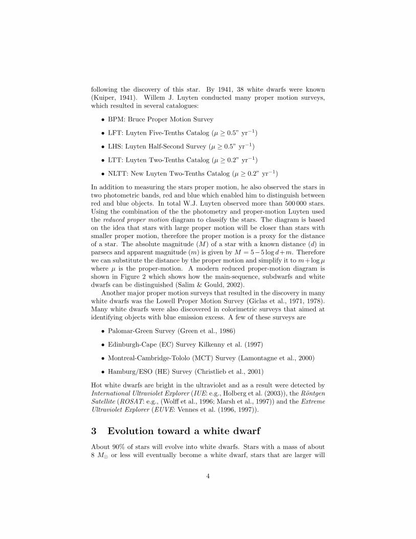
The first white dwarf to have its spectrum taken was 40 Eridani B (40 Eri B)as part the Henry-Draper Catalogue (Cannon & Pickering, 1918). Henry NorrisRussell plotted the absolute magnitude versus the spectral type and noted theoutstanding point in the plot. Figure 3 shows the original plot of H.R. Russell(Russell, 1914). The outstanding point is 40 Eri B which classified an A star, but

1At the same time he noticed that Procyon was showing the same behavior.2Procyon B was first observed in 1986 by John M. Schaeberle using the 36-inch telescope

at Lick Observatory.

1

H.N. Russell disregarded this because its ”spectrum is very doubtful” (Russell,1913). 3 In the same year Walter S. Adams noted its peculiarity (Adams, 1914).

The first spectrum of Sirius B was obtained in 1914 by Walter S. Adamsusing the 60-inch telescope at Mt. Wilson Observatory (Adams, 1915). As aresult he gave Sirius B the classification of an A-type star, same as 40 Eridani B,the only other known white dwarf at that time. Adams (1925) obtained a secondspectrum using the 100-inch telescope and used it to measure a gravitationalredshift of 21 km s−1 (Adams, 1925), which was in agreement with Arthur S.Eddington’s predicted value of 20 km s−1 (Eddington, 1924). Note, that eventhough Eddington has taken into account general relativity to calculate thegravitational redshift, Eddington assumed a structure for the white dwarf waswrong.

In 1926, Enrico Fermi and Paul Dirac showed that electrons obey what isnow called the Fermi-Dirac statistics, which take into account the Pauli exclu-sion principle. And in the same year Ralph H. Fowler (Fowler, 1926) applied thisnew rule to white dwarf stars and showed that the pressure supporting whitedwarfs against gravity is the electron degenerate pressure. Taking this theoryfurther Subrahmanyan Chandrasekhar extended Fowler’s work by including gen-eral relativity in the calculations and showed that there exists an upper limit onthe mass of a white dwarf (Chandrasekhar, 1935). The derivation of the whitedwarf structure is discussed in more detail in § 6.

When Chandrasekhar’s structure for a white dwarf is adopted, a mass of1.0 M� for Sirius B results in a radius of 0.008 R�. The gravitational redshiftcan be calculated using:

v

c=

∆λ

λ=

GM

c2R

which results in vg = 78 km s−1, which is much larger than the value measuredby Adams. A new gravitational redshift of 89±16 km s−1 was obtained in 1971by Greenstein et al.. This value is now in agreement with the predicted value,so why did Adams obtain a value that is so low? Wesemael (1985) showed thatAdams’ spectrum was heavily contaminated by Sirius A.

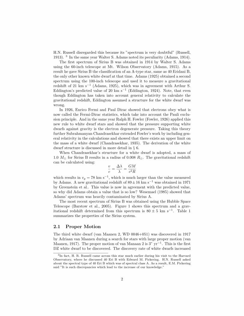
The most recent spectrum of Sirius B was obtained using the Hubble SpaceTelescope (Barstow et al., 2005). Figure 1 shows this spectrum and a grav-itational redshift determined from this spectrum is 80 ± 5 km s−1. Table 1summarizes the properties of the Sirius system.

2.1 Proper Motion

The third white dwarf (van Maanen 2, WD 0046+051) was discovered in 1917by Adriaan van Maanen during a search for stars with large proper motion (vanMaanen, 1917). The proper motion of van Manaan 2 is 3” yr−1. This is the firstDZ white dwarf to be discovered. The discovery rate of white dwarfs increased

3In fact, H. R. Russell came across this star much earlier during his visit to the HarvardObservatory, where he discussed 40 Eri B with Edward M. Pickering. H.N. Russell askedabout the spectral type of 40 Eri B which was of spectral class A. As a result, E.M. Pickeringsaid ”It is such discrepancies which lead to the increase of our knowledge.”

2

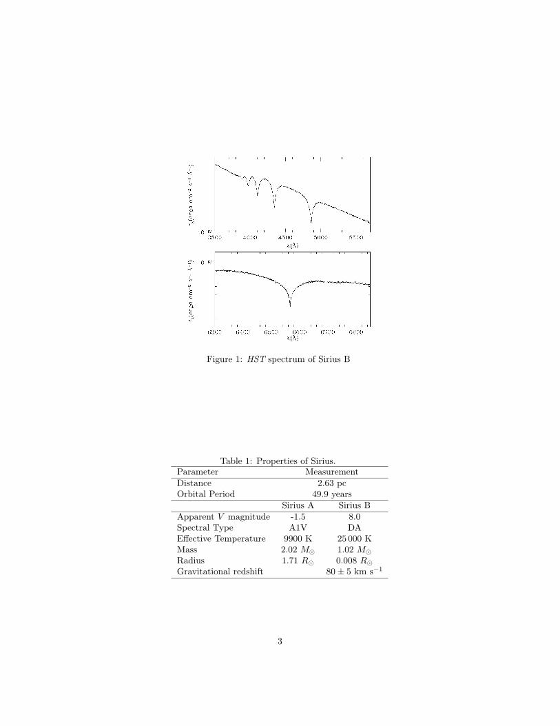
Figure 1: HST spectrum of Sirius B

Table 1: Properties of Sirius.Parameter MeasurementDistance 2.63 pcOrbital Period 49.9 years

Sirius A Sirius BApparent V magnitude -1.5 8.0Spectral Type A1V DAEffective Temperature 9900 K 25 000 KMass 2.02 M� 1.02 M�Radius 1.71 R� 0.008 R�Gravitational redshift 80± 5 km s−1

3

following the discovery of this star. By 1941, 38 white dwarfs were known(Kuiper, 1941). Willem J. Luyten conducted many proper motion surveys,which resulted in several catalogues:

• BPM: Bruce Proper Motion Survey

• LFT: Luyten Five-Tenths Catalog (µ ≥ 0.5” yr−1)

• LHS: Luyten Half-Second Survey (µ ≥ 0.5” yr−1)

• LTT: Luyten Two-Tenths Catalog (µ ≥ 0.2” yr−1)

• NLTT: New Luyten Two-Tenths Catalog (µ ≥ 0.2” yr−1)

In addition to measuring the stars proper motion, he also observed the stars intwo photometric bands, red and blue which enabled him to distinguish betweenred and blue objects. In total W.J. Luyten observed more than 500 000 stars.Using the combination of the the photometry and proper-motion Luyten usedthe reduced proper motion diagram to classify the stars. The diagram is basedon the idea that stars with large proper motion will be closer than stars withsmaller proper motion, therefore the proper motion is a proxy for the distanceof a star. The absolute magnitude (M) of a star with a known distance (d) inparsecs and apparent magnitude (m) is given by M = 5−5 log d+m. Thereforewe can substitute the distance by the proper motion and simplify it to m+log µwhere µ is the proper-motion. A modern reduced proper-motion diagram isshown in Figure 2 which shows how the main-sequence, subdwarfs and whitedwarfs can be distinguished (Salim & Gould, 2002).

Another major proper motion surveys that resulted in the discovery in manywhite dwarfs was the Lowell Proper Motion Survey (Giclas et al., 1971, 1978).Many white dwarfs were also discovered in colorimetric surveys that aimed atidentifying objects with blue emission excess. A few of these surveys are

• Palomar-Green Survey (Green et al., 1986)

• Edinburgh-Cape (EC) Survey Kilkenny et al. (1997)

• Montreal-Cambridge-Tololo (MCT) Survey (Lamontagne et al., 2000)

• Hamburg/ESO (HE) Survey (Christlieb et al., 2001)

Hot white dwarfs are bright in the ultraviolet and as a result were detected byInternational Ultraviolet Explorer (IUE: e.g., Holberg et al. (2003)), the RontgenSatellite (ROSAT: e.g., (Wolff et al., 1996; Marsh et al., 1997)) and the ExtremeUltraviolet Explorer (EUVE: Vennes et al. (1996, 1997)).

3 Evolution toward a white dwarf

About 90% of stars will evolve into white dwarfs. Stars with a mass of about8 M� or less will eventually become a white dwarf, stars that are larger will

4

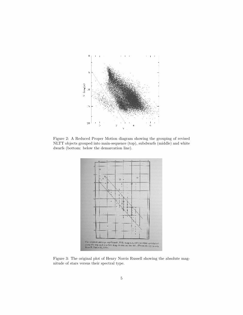
Figure 2: A Reduced Proper Motion diagram showing the grouping of revisedNLTT objects grouped into main-sequence (top), subdwarfs (middle) and whitedwarfs (bottom: below the demarcation line).

Figure 3: The original plot of Henry Norris Russell showing the absolute mag-nitude of stars versus their spectral type.

5

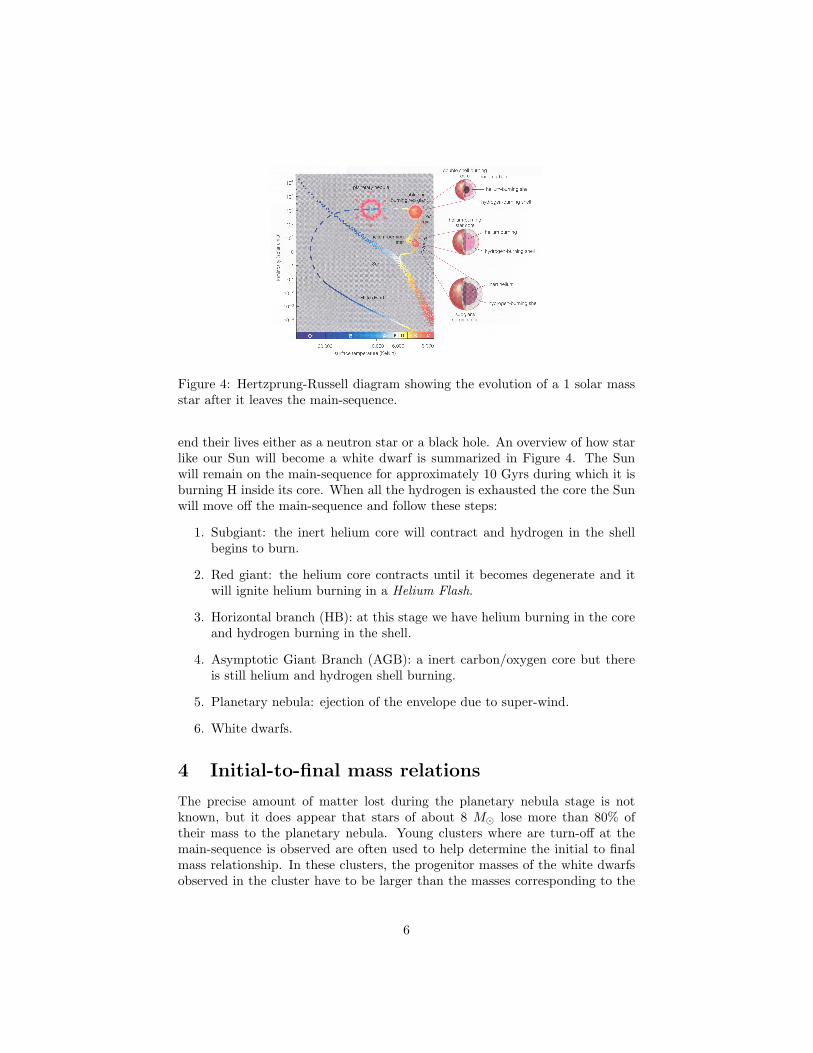
Figure 4: Hertzprung-Russell diagram showing the evolution of a 1 solar massstar after it leaves the main-sequence.

end their lives either as a neutron star or a black hole. An overview of how starlike our Sun will become a white dwarf is summarized in Figure 4. The Sunwill remain on the main-sequence for approximately 10 Gyrs during which it isburning H inside its core. When all the hydrogen is exhausted the core the Sunwill move off the main-sequence and follow these steps:

1. Subgiant: the inert helium core will contract and hydrogen in the shellbegins to burn.

2. Red giant: the helium core contracts until it becomes degenerate and itwill ignite helium burning in a Helium Flash.

3. Horizontal branch (HB): at this stage we have helium burning in the coreand hydrogen burning in the shell.

4. Asymptotic Giant Branch (AGB): a inert carbon/oxygen core but thereis still helium and hydrogen shell burning.

5. Planetary nebula: ejection of the envelope due to super-wind.

6. White dwarfs.

4 Initial-to-final mass relations

The precise amount of matter lost during the planetary nebula stage is notknown, but it does appear that stars of about 8 M� lose more than 80% oftheir mass to the planetary nebula. Young clusters where are turn-off at themain-sequence is observed are often used to help determine the initial to finalmass relationship. In these clusters, the progenitor masses of the white dwarfsobserved in the cluster have to be larger than the masses corresponding to the

6

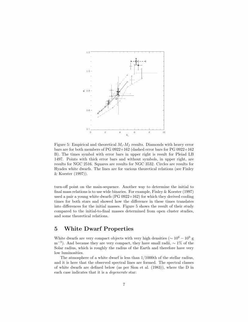
Figure 5: Empirical and theoretical Mi-Mf results. Diamonds with heavy errorbars are for both members of PG 0922+162 (dashed error bars for PG 0922+162B). The times symbol with error bars in upper right is result for Pleiad LB1497. Points with thick error bars and without symbols, in upper right, areresults for NGC 2516. Squares are results for NGC 3532. Circles are results forHyades white dwarfs. The lines are for various theoretical relations (see Finley& Koester (1997)).

turn-off point on the main-sequence. Another way to determine the initial tofinal mass relations is to use wide binaries. For example, Finley & Koester (1997)used a pair a young white dwarfs (PG 0922+162) for which they derived coolingtimes for both stars and showed how the difference in these times translatesinto differences for the initial masses. Figure 5 shows the result of their studycompared to the initial-to-final masses determined from open cluster studies,and some theoretical relations.

5 White Dwarf Properties

White dwarfs are very compact objects with very high densities (∼ 106 − 109 gm−3). And because they are very compact, they have small radii, ∼ 1% of theSolar radius, which is roughly the radius of the Earth and therefore have verylow luminosities.

The atmosphere of a white dwarf is less than 1/1000th of the stellar radius,and it is here that the observed spectral lines are formed. The spectral classesof white dwarfs are defined below (as per Sion et al. (1983)), where the D ineach case indicates that it is a degenerate star:

7

DA stars are hydrogen-rich showing H lines.

DO stars are helium-rich showing He II lines.

DB stars are helium-rich showing He I lines.

DC stars are helium-rich which a continuous spectrum.

DQ stars are helium-rich showing carbon features that can be either atomicor molecular.

DZ stars are helium-rich and show metal lines, for example the most commonlydetected metals are Ca, Na, Mg, and Fe.

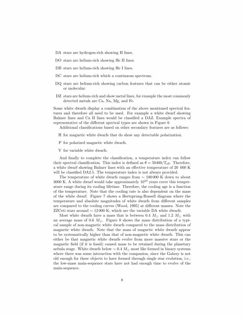
Some white dwarfs display a combination of the above mentioned spectral fea-tures and therefore all need to be used. For example a white dwarf showingBalmer lines and Ca II lines would be classified a DAZ. Example spectra ofrepresentative of the different spectral types are shown in Figure 6

Additional classifications based on other secondary features are as follows:

H for magnetic white dwarfs that do show any detectable polarization.

P for polarized magnetic white dwarfs.

V for variable white dwarfs.

And finally to complete the classification, a temperature index can followtheir spectral classification. This index is defined as θ = 50400/Teff . Therefore,a white dwarf showing Balmer lines with an effective temperature of 20 000 Kwill be classified DA2.5. The temperature index is not always provided.

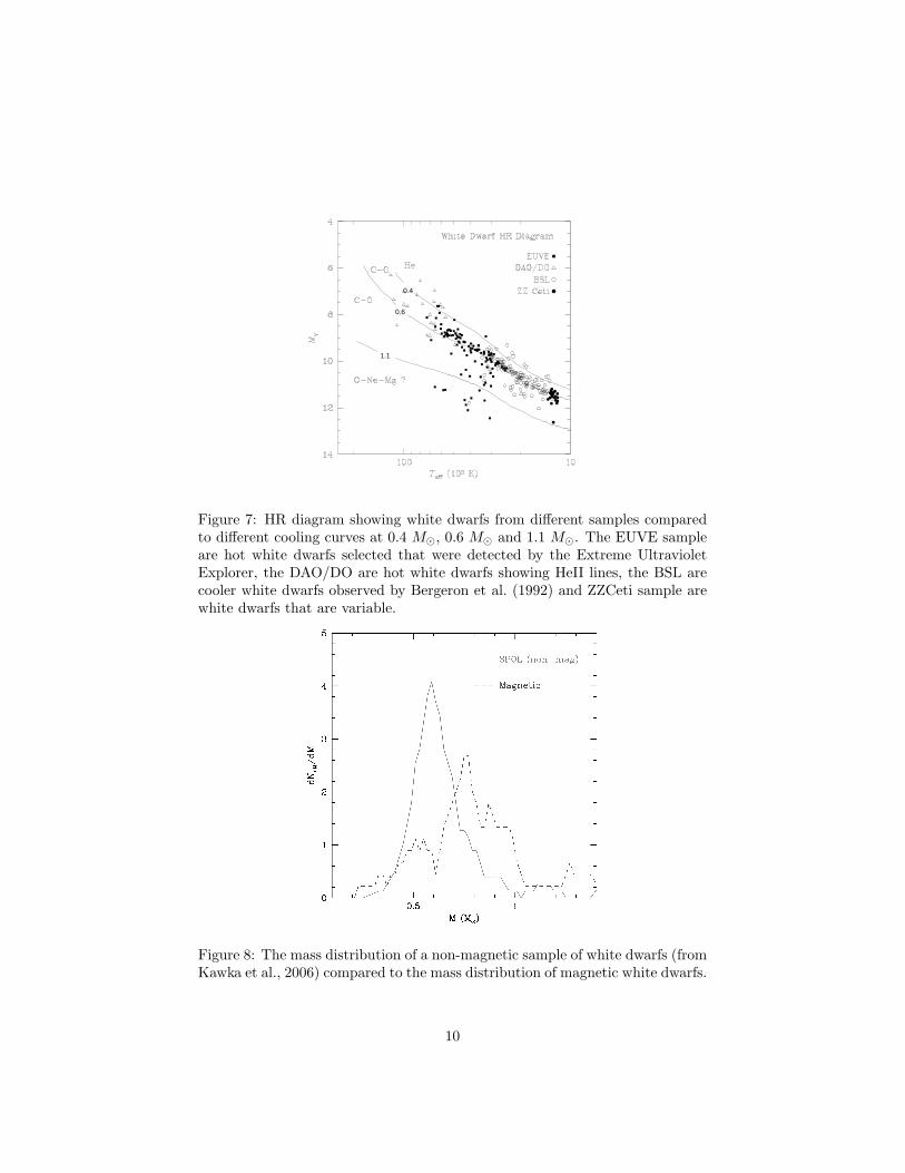
The temperature of white dwarfs ranges from ∼ 100 000 K down to about3000 K. A white dwarf would take approximately 1010 years cover this temper-ature range during its cooling lifetime. Therefore, the cooling age is a functionof the temperature. Note that the cooling rate is also dependent on the massof the white dwarf. Figure 7 shows a Hertzprung-Russell diagram where thetemperature and absolute magnitudes of white dwarfs from different samplesare compared to the cooling curves (Wood, 1995) at different masses. Note theZZCeti stars around ∼ 12 000 K, which are the variable DA white dwarfs.

Most white dwarfs have a mass that is between 0.4 M� and 1.2 M� withan average mass of 0.6 M�. Figure 8 shows the mass distribution of a typi-cal sample of non-magnetic white dwarfs compared to the mass distribution ofmagnetic white dwarfs. Note that the mass of magnetic white dwarfs appearto be systematically higher than that of non-magnetic white dwarfs. This caneither be that magnetic white dwarfs evolve from more massive stars or themagnetic field (if it is fossil) caused mass to be retained during the planetarynebula stage. White dwarfs below ∼ 0.4 M� most like formed in binary systemswhere there was some interaction with the companion, since the Galaxy is notold enough for these objects to have formed through single star evolution, i.e.,the low-mass main-sequence stars have not had enough time to evolve of themain-sequence.

8

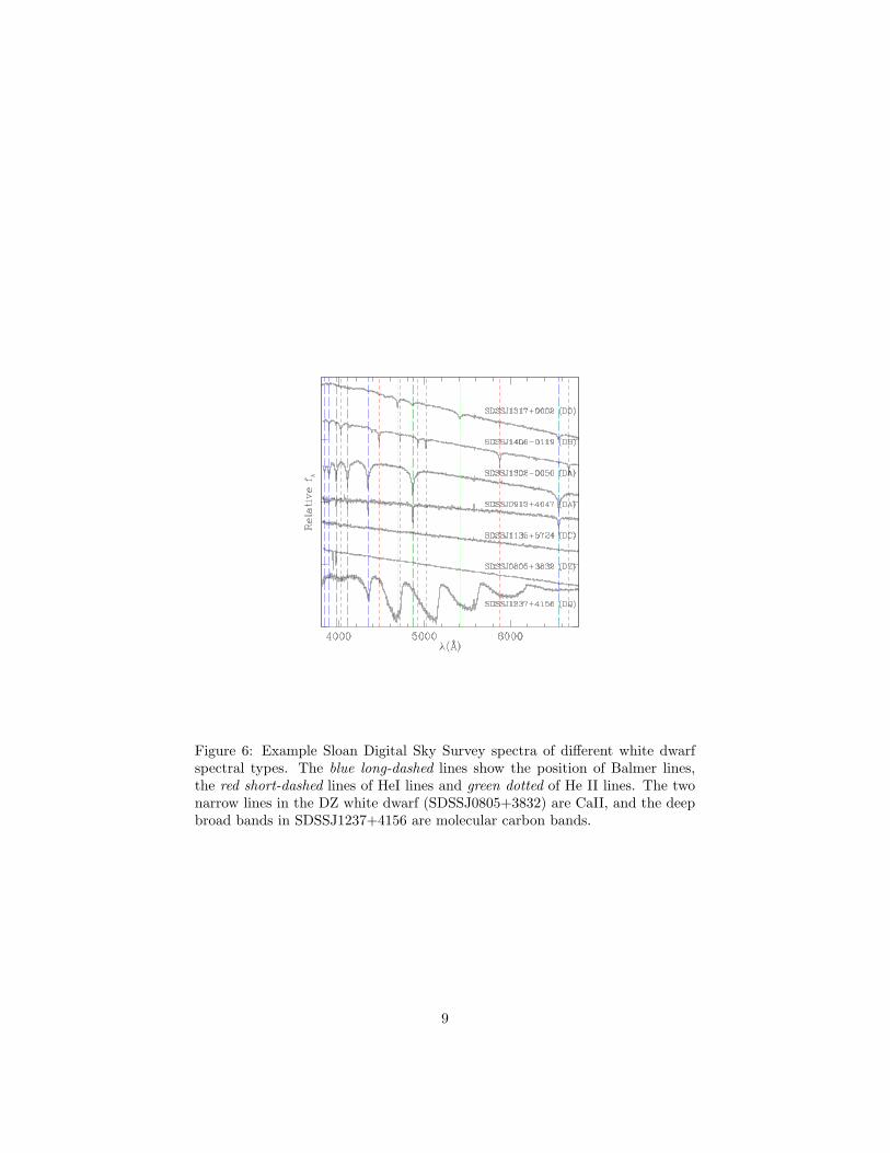
Figure 6: Example Sloan Digital Sky Survey spectra of different white dwarfspectral types. The blue long-dashed lines show the position of Balmer lines,the red short-dashed lines of HeI lines and green dotted of He II lines. The twonarrow lines in the DZ white dwarf (SDSSJ0805+3832) are CaII, and the deepbroad bands in SDSSJ1237+4156 are molecular carbon bands.

9

0.6

0.4

1.1

Figure 7: HR diagram showing white dwarfs from different samples comparedto different cooling curves at 0.4 M�, 0.6 M� and 1.1 M�. The EUVE sampleare hot white dwarfs selected that were detected by the Extreme UltravioletExplorer, the DAO/DO are hot white dwarfs showing HeII lines, the BSL arecooler white dwarfs observed by Bergeron et al. (1992) and ZZCeti sample arewhite dwarfs that are variable.

Figure 8: The mass distribution of a non-magnetic sample of white dwarfs (fromKawka et al., 2006) compared to the mass distribution of magnetic white dwarfs.

10

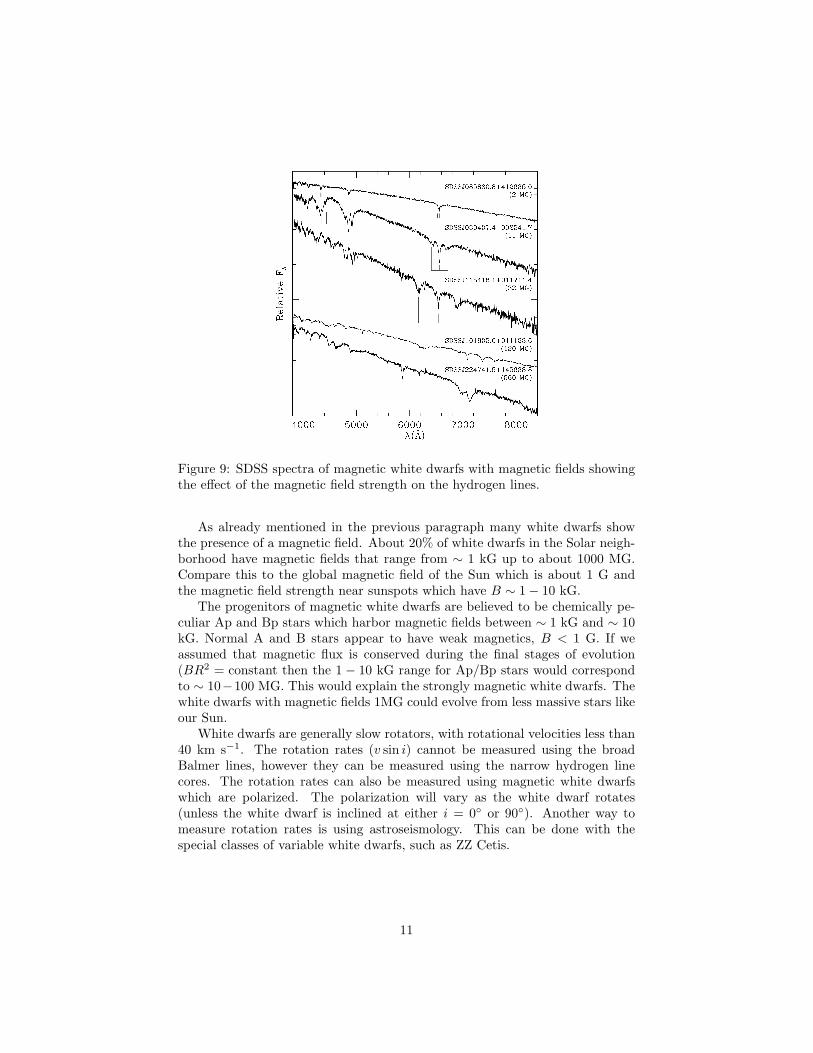
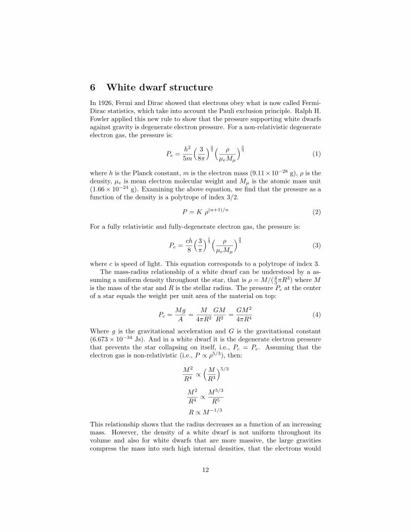
Figure 9: SDSS spectra of magnetic white dwarfs with magnetic fields showingthe effect of the magnetic field strength on the hydrogen lines.

As already mentioned in the previous paragraph many white dwarfs showthe presence of a magnetic field. About 20% of white dwarfs in the Solar neigh-borhood have magnetic fields that range from ∼ 1 kG up to about 1000 MG.Compare this to the global magnetic field of the Sun which is about 1 G andthe magnetic field strength near sunspots which have B ∼ 1− 10 kG.

The progenitors of magnetic white dwarfs are believed to be chemically pe-culiar Ap and Bp stars which harbor magnetic fields between ∼ 1 kG and ∼ 10kG. Normal A and B stars appear to have weak magnetics, B < 1 G. If weassumed that magnetic flux is conserved during the final stages of evolution(BR2 = constant then the 1 − 10 kG range for Ap/Bp stars would correspondto ∼ 10−100 MG. This would explain the strongly magnetic white dwarfs. Thewhite dwarfs with magnetic fields 1MG could evolve from less massive stars likeour Sun.

White dwarfs are generally slow rotators, with rotational velocities less than40 km s−1. The rotation rates (v sin i) cannot be measured using the broadBalmer lines, however they can be measured using the narrow hydrogen linecores. The rotation rates can also be measured using magnetic white dwarfswhich are polarized. The polarization will vary as the white dwarf rotates(unless the white dwarf is inclined at either i = 0◦ or 90◦). Another way tomeasure rotation rates is using astroseismology. This can be done with thespecial classes of variable white dwarfs, such as ZZ Cetis.

11

6 White dwarf structure

In 1926, Fermi and Dirac showed that electrons obey what is now called Fermi-Dirac statistics, which take into account the Pauli exclusion principle. Ralph H.Fowler applied this new rule to show that the pressure supporting white dwarfsagainst gravity is degenerate electron pressure. For a non-relativistic degenerateelectron gas, the pressure is:

Pe =h2

5m

( 38π

) 23( ρ

µeMµ

) 53

(1)

where h is the Planck constant, m is the electron mass (9.11×10−28 g), ρ is thedensity, µe is mean electron molecular weight and Mµ is the atomic mass unit(1.66× 10−24 g). Examining the above equation, we find that the pressure as afunction of the density is a polytrope of index 3/2.

P = K ρ(n+1)/n (2)

For a fully relativistic and fully-degenerate electron gas, the pressure is:

Pe =ch

8

( 3π

) 13( ρ

µeMµ

) 43

(3)

where c is speed of light. This equation corresponds to a polytrope of index 3.The mass-radius relationship of a white dwarf can be understood by a as-

suming a uniform density throughout the star, that is ρ = M/( 43πR3) where M

is the mass of the star and R is the stellar radius. The pressure Pc at the centerof a star equals the weight per unit area of the material on top:

Pc =Mg

A=

M

4πR2

GM

R2=

GM2

4πR4(4)

Where g is the gravitational acceleration and G is the gravitational constant(6.673× 10−34 Js). And in a white dwarf it is the degenerate electron pressurethat prevents the star collapsing on itself, i.e., Pc = Pe. Assuming that theelectron gas is non-relativistic (i.e., P ∝ ρ5/3), then:

M2

R4∝

( M

R3

)5/3

M2

R4∝ M5/3

R5

R ∝M−1/3

This relationship shows that the radius decreases as a function of an increasingmass. However, the density of a white dwarf is not uniform throughout itsvolume and also for white dwarfs that are more massive, the large gravitiescompress the mass into such high internal densities, that the electrons would

12

gain very high momenta and hence velocities that begin to approach the speedof light. Under these conditions it is necessary to adopt the fully relativisticand degenerate equation for the pressure of the electron gas (Pe ∝ ρ4/3).

To determine the structure of a star, we require that the star is in a hydro-static equilibrium:

dP

dr= −ρ g = −ρ

G M(r)r2

(5)

where M(r) is the mass of the star at radius r. We also require the equation ofmass continuity which ensures mass conservation.

M(r)dr

= 4πr2ρ (6)

To solve the structure of a white dwarf, we need to combine the mass conti-nuity (Eqn. 6) and the hydrostatic equilibrium (Eqn. 5) equations. Equation 5can be re-written as:

r2

ρ

dP

dr= −GM(r)

and differentiating both side with respect to r, we get:

d

dr

(r2

ρ

dP

dr

)= −G

dM(r)dr

Here, we can insert the mass continuity equation:

d

dr

(r2

ρ

dP

dr

)= −G 4πr2ρ

1r2

d

dr

(r2

ρ

dP

dr

)= −4πGρ (7)

Lane and Emden suggested that a family of solutions may be obtained if oneassumes that the pressure as a function of the density is a polytropic function(Eqn.2). Equations 1 and 3 are polytropes of indices n = 3/2 and 3, respectively.

To solve the Lane-Emden (L.E.) equation, we first scale ρ:

ρ = λΦn (8)

where λ is a scaling factor. The pressure becomes:

P = K(λΦn)(n+1)/n = Kλ(n+1)/nΦn+1

which we substitute into the L.E. equation (Eqn. 7).

1r2

d

dr

( r2

λΦn

d(Kλ(n+1)/nΦn+1)dr

)= −4πGλΦn

1r2

d

dr

( r2

λΦnKλ(n+1)/n(n + 1)Φn dΦ

dr

)= −4πGλΦn

13

which when simplified results in:

Kλ(1−n)/n(n + 1)4πG

1r2

d

dr

(r2 dΦ

dr

)= −Φn (9)

Here, we can define the ”length” a:

a2 =Kλ(1−n)/n(n + 1)

4πG(10)

and when substituted into Equation 9 we get:

a2

r2

d

dr

(r2 dΦ

dr

)= −Φn (11)

Finally we define a dimensionless scaling factor, ξ = r/a, and the L.E. equationbecomes:

1ξ2

d

dξ

(ξ2 dΦ

dξ

)= −Φn (12)

At this point we can define the boundary conditions. At the center of the star(ξ = 0 and hence r = 0), the scaling factor λ = ρc will be the central densityand Φ = 1, i.e., Φ = 1 and ρ = λΦn = ρc at ξ = 0. Rearrange, Equation 12 anddifferentiate:

d

dξ

(ξ2 dΦ

dξ

)= −Φnξ2

2ξdΦdξ

+ ξ2 d2Φdξ2

= −Φnξ2

2dΦdξ

+ ξd2Φdξ2

= −Φnξ

And evaluating at ξ = 0, we get:

dΦdξ

= 0

which becomes the second boundary condition. Now with the zeroth and firstderivatives at ξ = 0 we can integrate outward (e.g., using the Runge-Kutta) andevaluate these functions until we reach the first zero of Φ which corresponds toρ = 0, that is the surface of the star, where

Φ(ξ1) = 0

and therefore the stellar radius will be:

R = aξ1 =

√(n + 1)Kλ(1−n)/n

4πGξ1 (13)

To obtain the mass of the star we integrate the mass-continuity equation (Eqn. 6):

dM = 4πr2ρdr

14

into which we substitute for r and ρ:

dM = 4π(aξ)2(λΦn)adξ = 4πa3λΦnξ2dξ (14)

and using the L.E. equation (i.e., Eqn. 12) which we rewrite as:

Φnξ2dξ = −d(ξ2 dΦ

dξ

)We now substitute this equation into Eqn. 14 to get:

dM = −4πa3λd(ξ2 dΦ

dξ

)Which can now be integrated from M(ξ = 0) = 0 to M(ξ):

M(ξ) = −4πa3λξ2 dΦdξ

(15)

And the total mass of the star will be:

M(R) = M(ξ1)

Analytical solutions exist for n = 0, 1, 5, however values for n = 3/2, 3 arenumerical.

Figure 10 shows the calculated structure of white dwarf with a total mass of0.6 M�, where the density and integrated mass are plotted as a function of theradius. The Runge-Kutta 4th order integration method was used with a centraldensity of ρc = 3.39× 106 g cm−3 which one of the initial boundary conditions.In the calculation, the mean electron molecular weight needs to be defined, andfor fully ionized He, C, N or O, µe = 2.0, which is the value that was adopted.The intergration was conducted until the total mass was well converged and theradius of a 0.6 M� was found to be 0.0105 R�.

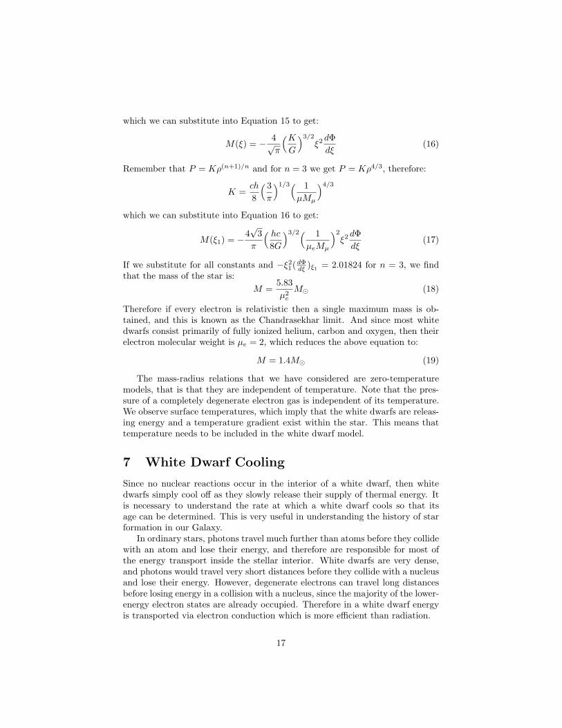
Repeating the integration for different central densities and hence obtainingdifferent masses, we can calculate the mass-radius relation for white dwarfs.Figure 11 shows the mass-radius relation for white dwarfs where we assumeµ = 2.0 and µ = 2.151 (for fully ionized iron). These mass radius relations arealso compared to the simple relation, where R ∝M−1/3.

For a white dwarf star that has a fully relativistic and degenerate electrongas we defined the pressure in Equation 3, that is:

Pe =ch

8

( 3π

) 13( ρ

µe Mµ

) 43

Also the definition for a in Equation 10, which for n = 3 becomes:

a =1

λ1/3

√K

πG

15

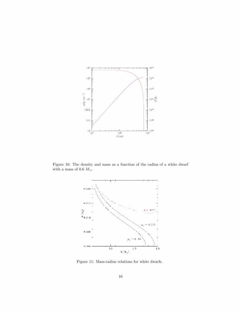
Figure 10: The density and mass as a function of the radius of a white dwarfwith a mass of 0.6 M�.

Figure 11: Mass-radius relations for white dwarfs.

16

which we can substitute into Equation 15 to get:

M(ξ) = − 4√π

(K

G

)3/2

ξ2 dΦdξ

(16)

Remember that P = Kρ(n+1)/n and for n = 3 we get P = Kρ4/3, therefore:

K =ch

8

( 3π

)1/3( 1µMµ

)4/3

which we can substitute into Equation 16 to get:

M(ξ1) = −4√

3π

( hc

8G

)3/2( 1µeMµ

)2

ξ2 dΦdξ

(17)

If we substitute for all constants and −ξ21(dΦ

dξ )ξ1 = 2.01824 for n = 3, we findthat the mass of the star is:

M =5.83µ2

e

M� (18)

Therefore if every electron is relativistic then a single maximum mass is ob-tained, and this is known as the Chandrasekhar limit. And since most whitedwarfs consist primarily of fully ionized helium, carbon and oxygen, then theirelectron molecular weight is µe = 2, which reduces the above equation to:

M = 1.4M� (19)

The mass-radius relations that we have considered are zero-temperaturemodels, that is that they are independent of temperature. Note that the pres-sure of a completely degenerate electron gas is independent of its temperature.We observe surface temperatures, which imply that the white dwarfs are releas-ing energy and a temperature gradient exist within the star. This means thattemperature needs to be included in the white dwarf model.

7 White Dwarf Cooling

Since no nuclear reactions occur in the interior of a white dwarf, then whitedwarfs simply cool off as they slowly release their supply of thermal energy. Itis necessary to understand the rate at which a white dwarf cools so that itsage can be determined. This is very useful in understanding the history of starformation in our Galaxy.

In ordinary stars, photons travel much further than atoms before they collidewith an atom and lose their energy, and therefore are responsible for most ofthe energy transport inside the stellar interior. White dwarfs are very dense,and photons would travel very short distances before they collide with a nucleusand lose their energy. However, degenerate electrons can travel long distancesbefore losing energy in a collision with a nucleus, since the majority of the lower-energy electron states are already occupied. Therefore in a white dwarf energyis transported via electron conduction which is more efficient than radiation.

17

The modern theory of white dwarf cooling was established by Mestel (1952)who showed that the white dwarf loses its thermal energy through the thin layerof non-degenerate atmosphere.

Since white dwarfs lack nuclear processes as an energy source, the evolutionis simply driven by the rate of change of internal energy as heat is radiated out.From thermodynamics, the internal energy u is related to the entropy s of thesystem by du = Tds (at constant volume and number of particles). Thereforethe rate of energy dissipated as heat is:

du

dt= T

ds

dt= T

( ∂s

∂T

)ρ

∂T

∂t+ T

(∂s

∂ρ

)T

∂ρ

∂t(20)

The specific heat of a gas at constant volume is simply (∂u/∂T )V and if weassume that there is no gravitational contraction (i.e., ∂ρ/∂t = 0) then theabove equation simplifies to:

du

dt= cV

∂T

∂t(21)

In the interior of a white dwarf, the electrons are degenerate but the ions arenon-degenerate. The heat capacity per unit volume cV of a gas that consists ofnon-degenerate ions and non-relativistic electrons is:

cV =32nik +

π2

2nek

( kT

EF

)(22)

where EF is the Fermi energy, ni and ne are the number density of ions andelectrons, respectively, k is the Boltzmann constant and T is the temperatureof the gas. From the equation we can see that electrons do not contributesignificantly to the heat capacity inside the white dwarf because the electronsare strongly degenerate (i.e., EF � kT ).

Since the luminosity of a white dwarf star is maintained by the thermalenergy of ions, then the luminosity L is:

L = −dU

dt= − d

dt

∫ ∫cV dTdV (23)

We also require a relationship between the core temperature and the surfacetemperature in order to calculate an evolutionary scenario. The interior ofa white dwarf is isothermal due to the very high electron conductivity. Thetemperature change from the interior to the surface occurs within a thin layerof essentially non-degenerate gas. The energy transport through this layer isassumed to be due to radiative diffusion. The opacity κ of the gas in thislayer is caused by free-free and bound-free absorption and can be expressed byKramer’s law:

κ = κ0ρT−3.5 (24)

where κ0 is a constant that depends on the composition.To derive the pressure as a function of the temperature in these layers, we

need to combine the hydrostatic equilibrium equation (Equation 5) with the

18

equation for radiative transfer. In these layers, we assume that the mean freepath of a photon is much less than the temperature scale height, and thereforethe radiation is very close to that of a blackbody. Therefore the radiative transferin these layers is:

L

4πr2= − 4ac

3ρκT 3 dT

dr(25)

where a = 7.564× 10−15 erg cm−3 K−4. We can rearrange the above equationsuch that:

dr = −4πr2

L

4ac

3ρκT 3dT

which we substitute into the equation for hydrostatic equilibrium and obtain:

dP

dT=

4ac

3κ

4πGM

LT 3

and finally substituting in Kramer’s law for opacity (Eqn. 24) and simplifying:

dP

dT=

4ac

34πGM

Lρκ0T 6.5 (26)

Close to the surface of the white dwarf, the gas is non-degenerate and thepressure can be approximated by the pressure for an ideal gas. Here we assumethat the gas is fully ionized and the coulomb interaction energy is much lessthan the kinetic energy.

Pi =ρkT

µmp(27)

where mp is the mass of a proton, since we assume that the pressure is mostlyprovided by ionized hydrogen. We can now eliminate ρ from Equation 26 bysubstituting in Equation 27 to obtain:

PdP =4ac

34πGMk

Lκ0µmpT 7.5dT

Given that the photospheric temperature of the white dwarf is small compared tothe interior temperature we can integrate the above equation with the boundarycondition such that T = 0 at P = 0.

P 2 =2

8.54πGk

κ0µmp

M

LT 8.5

Now we substitute for pressure using Equation 27 and simplifying:

ρ =( 2

8.54ac

34πGM

κ0L

µmp

k

)1/2

T 3.25 (28)

To simplify further calculations, we will define:

K1 =( 2

8.54ac

34πG

κ0

µmp

k

)1/2

(29)

19

and therefore Equation 28 will become:

ρ = K1

(M

L

)1/2

T 3.25 (30)

This equation assumed a non-degenerate gas in its derivation, which becomes in-valid at densities where electron degeneracy becomes important. At the bound-ary of the isothermal core with the outer non-degenerate envelope, we assumethat the pressure of the non-degenerate electron gas is equal to the pressureof a completely degenerate electron gas (Eqn. 1) with a temperature of theisothermal core, Tc:

ρckTc

µeMµ=

h2

5m

( 38π

) 23( ρc

µeMµ

) 53

(31)

where ρc is the gas density at the core boundary. And rearranging to obtainthe density at the core boundary:

ρc =8π

3

(5mk

h2

)3/2

µeMµT 3/2c

ρc = K2T3/2c (32)

where

K2 =8π

3

(5mk

h2

)3/2

µeMµ (33)

And if we assume that Equation 30 is valid at the core boundary, i.e., ρ = ρc

and T = Tc, then:

K1

(M

L

)1/2

T 3.25c = K2T

3/2c

Solving for the luminosity to obtain:

L =(K1

K2

)2

MT 3.5c (34)

The available thermal energy of an isothermal white dwarf with a temper-ature Tc is provided mainly by the non-degenerate ions. The available thermalenergy is:

U =∫

cV TdV =∫

cV

ρdM ' cV

ρTcM

where cV and ρ are the mean values for the heat capacity cV and density ρ.Comparing this to Equation 23:

L = −dU

dt

Combining this equation with Equation 34 and our approximation for the avail-able thermal energy in a white dwarf star, we get

−dU

dt=

(K1

K2

)2

MT 3.5c

20

− d

dt

(cV

ρTc

)=

(K1

K2

)2

T 3.5

Note that the mass M cancels out, and if we assume that the average heatcapacity cV is time independent, then the integral of the above equation wherethe initial temperature T0 occurs at some time t0 is:

−d(cV Tc

ρ

)=

(K1

K2

)2

T 3.5c dt

−d(cV

ρ

1T 2.5

c

)=

(K1

K2

)2

dt

25

cV

ρ

( 1T 2.5

− 1T 2.5

0

)=

(K1

K2

)2

(t− t0) =(K1

K2

)2

τ (35)

If we assume that that T � T0, then:

τ =25

(K2

K2

)2(cV

ρ

) 1T 2.5

c

and substituting in Equation 34 we get the relationship:

τ =25

(cV

ρ

)TcM

L(36)

and again substituting in Equation 34, we can eliminate Tc and obtain:

τ =25

cV

ρ

(K2

K1

)4/7(M

L

)5/7

(37)

Here τ is the so called cooling age, that is the time required for the luminosityof a white dwarf to go from L0 to L, where we have assumed L0 to be verylarge compared to L when we assumed that T � T0. Rearranging of the aboveequation and making the relevant substitutions for the mean density, meanspecific heat, opacity, and constants, we can find the luminosity as a functionof the cooling age:

L ≈ 8.4× 10−4L�(M/M�) τ−7/59 (38)

where τ9 is the cooling age in 109 years.This simple power-law cooling model shows the basics of how a white dwarf

cools and it is a good approximation to more detailed cooling models. This isthe simplest view of how white dwarfs cool. However, the cooling history of awhite dwarf is more complex. And to construct a more representative model ofwhite dwarf cooling we need to consider several more elements.

The above model only considers the release of thermal energy, however as awhite dwarf cools there are additional energy sources that need to be considered.These will be briefly discussed below:

21

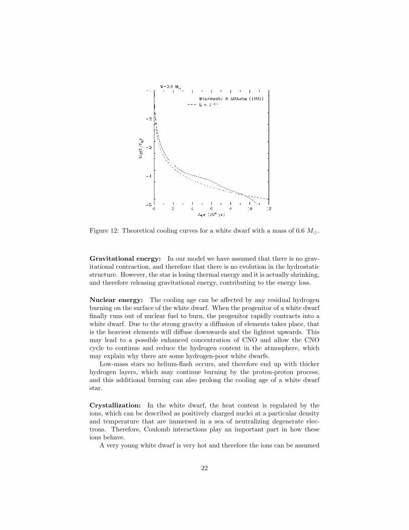
Figure 12: Theoretical cooling curves for a white dwarf with a mass of 0.6 M�.

Gravitational energy: In our model we have assumed that there is no grav-itational contraction, and therefore that there is no evolution in the hydrostaticstructure. However, the star is losing thermal energy and it is actually shrinking,and therefore releasing gravitational energy, contributing to the energy loss.

Nuclear energy: The cooling age can be affected by any residual hydrogenburning on the surface of the white dwarf. When the progenitor of a white dwarffinally runs out of nuclear fuel to burn, the progenitor rapidly contracts into awhite dwarf. Due to the strong gravity a diffusion of elements takes place, thatis the heaviest elements will diffuse downwards and the lightest upwards. Thismay lead to a possible enhanced concentration of CNO and allow the CNOcycle to continue and reduce the hydrogen content in the atmosphere, whichmay explain why there are some hydrogen-poor white dwarfs.

Low-mass stars no helium-flash occurs, and therefore end up with thickerhydrogen layers, which may continue burning by the proton-proton process,and this additional burning can also prolong the cooling age of a white dwarfstar.

Crystallization: In the white dwarf, the heat content is regulated by theions, which can be described as positively charged nuclei at a particular densityand temperature that are immersed in a sea of neutralizing degenerate elec-trons. Therefore, Coulomb interactions play an important part in how theseions behave.

A very young white dwarf is very hot and therefore the ions can be assumed

22

to behave like an ideal gas, however as it cools down, it will begin to crystallizefrom the center outwards. When this begins to occur, the ions are essentiallychanging phase, and therefore release latent heat during crystallization. Thisslows the white dwarf’s cooling and can be observed as an upturned bumpin the cooling curve. Figure 12 compares the cooling curve that was derivedabove (i.e., Eqn. 37) to a model cooling curve (Benvenuto & Althaus, 1999)that includes crystallization and other effects. Once the interior of the whitedwarf has crystallized and the temperature continues to decrease, the crystallinestructure accelerates the cooling. That is the vibration of the regularly spacednuclei promotes energy loss. This can be observed in Figure 12 as the sharpdownturn in the cooling curve.

The evolution of a white dwarf is not only determined by the available energysources but also by the processes that transport the energy to the surface. Thestructure of a white dwarf can be separated into the core where the electrons aredegenerate and the thin, non-degenerate envelope. Even though this envelope isvery thin and its mass is a very small fraction of the white dwarfs total mass, itis here where the energy transport is slowest and hence determines the coolingrate.

We have already mentioned that it is electron conduction that is responsiblefor energy transport inside the white dwarf core. However, the early and hencehot stages of white dwarf evolution is dominated by neutrino losses. Neutrinoluminosity is not dominant in the final stages of AGB evolution, however it isimportant, so when the white dwarf starts to collapse following the end of shellburning, the photon luminosity drops, but the neutrino luminosity does. Herethe neutrino luminosity is driven by the central temperature of the white dwarf.

The energy transport in the thin, non-degenerate envelope can be either viaradiative transport and/or convective energy transport for cooler white dwarfs.The temperature at which a convective zone develops depends on the composi-tion of the thin non-degenerate envelope (atmosphere).

8 Model Atmospheres

The atmosphere of a star consists of the layers of the star that can be observed.The thickness of the atmosphere of a white dwarf does not exceed 1/1000th ofa stellar radius in thickness (hatmos/Rstar < 10−3) from which radiation escapesinto the vacuum of space. We can model the atmosphere by solving a set ofequations which will provide a physical description of the observable region ofa star. Since the thickness of the atmosphere of a white dwarf is much smallerthan the radius of the star, we can assume plane-parallel geometry, that is thegeometry of the atmosphere is unidimensional and parametrized by the heightz.

The radiated flux emitted at the surface of the star is frequency dependentand is expressed as the Eddington flux, Hν(z = z0), where z0 indicates thesurface, and carries the units erg cm−2 s−1 Hz−1 steradian−1. The total flux

23

emitted by the star is given by integrating over all solid angles and frequencies:

Ftotal = 4πHtotal = 4π

∫ ∞

0

Hνdν = σR T 4eff , (39)

where σR = 5.67 × 10−5 erg cm−2 s−1 K−4 is the Stefan-Boltzmann constant,and the above equation defines Teff , the effective temperature.

The atmosphere can modeled by solving a set of non-linear equations, whichwill provide a physical description of the observable region of the star:

• Energy transfer, which can be either or both radiative and convective.

• Radiative equilibrium, which implies energy conservation within the at-mosphere. The energy that enters the atmosphere must be equal to theenergy leaving the atmosphere, that is no energy is created or lost insidethe atmosphere.

• Hydrostatic equilibrium, that is where the gas pressure balances the grav-itational forces.

• Equation of state, that is the population of the energy levels.

• Charge and particle conservation, where the total number of particles isconserved and that the net electric charge is zero.

We solve the problem numerically, and therefore we first need to choose theindependent variable. In this case, it is better to select the Lagrangian massm, which is the mass as a function of the depth (i.e., mass loading), ratherthan the optical depth. The optical depth τ is defined as the probability that aphoton will escape from a certain depth inside the star into space e−τ . Thereforethe optical depth increases from the surface inward. The reason for using msimplifies the equation for hydrostatic equilibrium. And the optical depth isrelated to the thickness dz at depth z by:

dτ = −χdz

however we wish to use the variable m in our calculations:

dm = −ρdz

where ρ is the density of the atmosphere. Combining the two equations we geta relationship between the mass loading and the optical depth.

dτ =χ

ρdm

Since the problem is being solved numerically, discrete variables need to beused. Therefore the atmosphere needs to be sliced into layers, and the spectruminto discrete frequencies. For example:

m −→ md (d = 1,ND)

24

T = T (md) −→ Td (d = 1,ND)

Hν −→ Hd,j (d = 1,ND; j = 1,NJ)

We can now define the equations that will be used. The energy transport inwhite dwarfs is mostly radiative transfer:

∂Hν

∂z= χν(Sν − Jν)

where Jν is the specific intensity and Sν is the source function and is definedby:

Sν =ην

χν

and ην is emissivity, and the equation represents the transfer of energy within alayer of the atmosphere dz taking into account absorption and emission at anygiven frequency. Integrating the radiative transfer equation over all frequenciesleads to the radiative equilibrium that is the conservation of energy.

∂H

∂z= 0 =

∫χν(Sν − Jν)dν

When calculating the flux throughout the atmosphere a boundary conditionneeds to be defined. We need the total flux leaving the surface to be (i.e., theboundary condition):

F = 4πH = 4π

∫ ∞

0

Hνdν = σRT 4eff

We also need the atmosphere to be in hydrostatic equilibrium.

dP

dz= −ρg −→ dP

dm= −g,

In the atmosphere we can assume that the particles follow the ideal gas law,and hence the pressure acting against gravitational contraction is:

PV = NkT −→ P = nkT

where N is the number of particles and therefore n = N/V is the particledensity.

The atmosphere needs to be in statistical equilibrium, where the ionizationfractions are described the Saha equation:

ni

ni+1=

ui

ui+1NeΦ(T )

where n and u are the number density and the partition function, respectively,of the ith and i + 1th ionization states, and Φ(T ) for hydrogen is:

Φ(T ) =( h2

2πmkT

)3/2

eχH/kT

25

where m is the electron mass, χH is the ionization potential of the hydrogenatom. The population levels are described by the Boltzmann equation. Thefraction of atoms at a particular excitation level j will be:

Nj

N=

gje−εj/kT

uj

where uj is the partition function (uj =∑

j gjeεj/kT ), gj is the statistical weight

(the number of states per energy unit), and εj is the excitation energy at levelj above the ground state. The Saha ionization equation and the Boltzmannexcitation equation can be combined to find the fraction of atoms in a givenionization or excitation state.

And finally, the net electric charge needs to be zero, i.e.,

−Ne + Np = 0

and we will assume no mass loss, and hence the total number particles need tobe also conserved:

Ntot = Np + Ne +nlev∑

i

Ni

where Ne is the number of electrons, Np the number of protons, and Ni thenumber of atoms at level i.

8.1 Opacities

In a white dwarf atmosphere, several absorption processes will determine theopacity of the gas and must be taken into account in solving the radiativetransfer equation. Since most white dwarfs are hydrogen-rich, we will considerthe absorption processes that can occur in an hydrogen gas.

• Absorption by neutral hydrogen between bound levels (bound-bound),that is between principal quantum numbers n = l (lower level) and n = u(upper level), where the energy of a level is given by En = 13.595eV/n2.

• Absorption by neutral hydrogen between a bound level and the continuum(bound-free), and between two free states (free-free).

• Bound-free and free-free absorption by the negative hydrogen ion (H−).

• Scattering of light by neutral hydrogen (HI - Rayleigh scattering) and byelectrons (e− - Thomson scattering).

Due to spontaneous decay, energy levels have a finite lifetime, and therefore, afinite energy width Γnat = ∆El/h, which is the natural width of a line expressedin frequency units. Other mechanisms contribute to the broadening of lines, suchas:

26

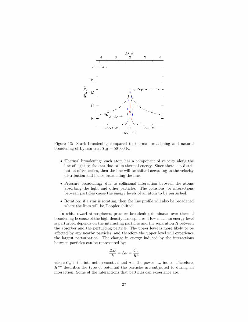
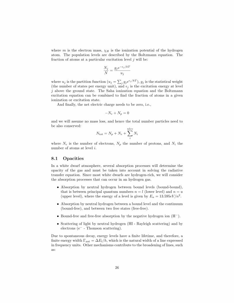
Figure 13: Stark broadening compared to thermal broadening and naturalbroadening of Lyman α at Teff = 50 000 K.

• Thermal broadening: each atom has a component of velocity along theline of sight to the star due to its thermal energy. Since there is a distri-bution of velocities, then the line will be shifted according to the velocitydistribution and hence broadening the line.

• Pressure broadening: due to collisional interaction between the atomsabsorbing the light and other particles. The collisions, or interactionsbetween particles cause the energy levels of an atom to be perturbed.

• Rotation: if a star is rotating, then the line profile will also be broadenedwhere the lines will be Doppler shifted.

In white dwarf atmospheres, pressure broadening dominates over thermalbroadening because of the high-density atmospheres. How much an energy levelis perturbed depends on the interacting particles and the separation R betweenthe absorber and the perturbing particle. The upper level is more likely to beaffected by any nearby particles, and therefore the upper level will experiencethe largest perturbation. The change in energy induced by the interactionsbetween particles can be represented by:

∆E

h= ∆ν =

Cn

Rn

where Cn is the interaction constant and n is the power-law index. Therefore,R−n describes the type of potential the particles are subjected to during aninteraction. Some of the interactions that particles can experience are:

27

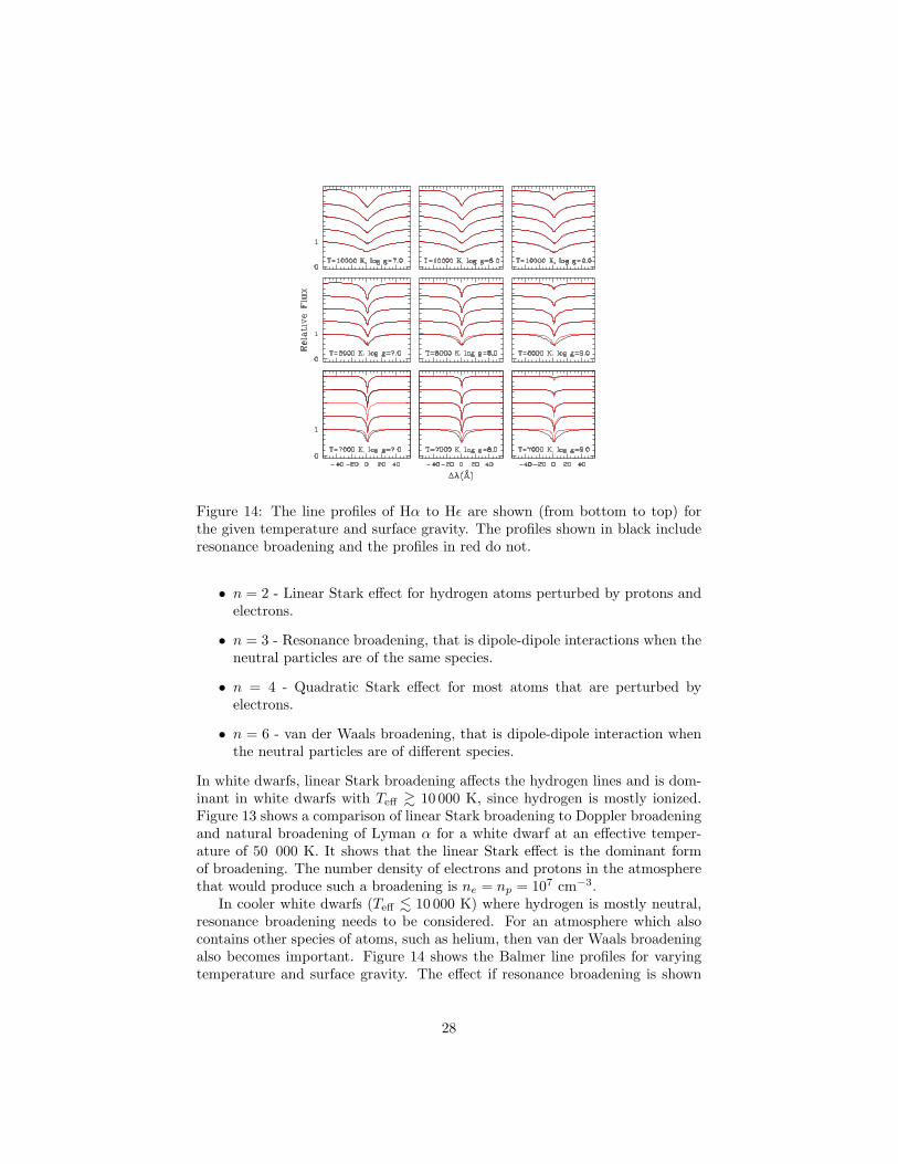
Figure 14: The line profiles of Hα to Hε are shown (from bottom to top) forthe given temperature and surface gravity. The profiles shown in black includeresonance broadening and the profiles in red do not.

• n = 2 - Linear Stark effect for hydrogen atoms perturbed by protons andelectrons.

• n = 3 - Resonance broadening, that is dipole-dipole interactions when theneutral particles are of the same species.

• n = 4 - Quadratic Stark effect for most atoms that are perturbed byelectrons.

• n = 6 - van der Waals broadening, that is dipole-dipole interaction whenthe neutral particles are of different species.

In white dwarfs, linear Stark broadening affects the hydrogen lines and is dom-inant in white dwarfs with Teff & 10 000 K, since hydrogen is mostly ionized.Figure 13 shows a comparison of linear Stark broadening to Doppler broadeningand natural broadening of Lyman α for a white dwarf at an effective temper-ature of 50 000 K. It shows that the linear Stark effect is the dominant formof broadening. The number density of electrons and protons in the atmospherethat would produce such a broadening is ne = np = 107 cm−3.

In cooler white dwarfs (Teff . 10 000 K) where hydrogen is mostly neutral,resonance broadening needs to be considered. For an atmosphere which alsocontains other species of atoms, such as helium, then van der Waals broadeningalso becomes important. Figure 14 shows the Balmer line profiles for varyingtemperature and surface gravity. The effect if resonance broadening is shown

28

Figure 15: Pulsating stars across the Hertzprung-Russell diagram.

by comparing spectral line profiles which include resonance broadening to lineswhich do not. Resonance broadening becomes prominent at lower temperatures(i.e., Teff ≤ 8000 K) where neutral hydrogen atoms are more numerous andmore likely to interact with the radiative atoms.

9 Variable White Dwarfs

The first pulsating star to be discovered was Mira (o Ceti). David Fabriciusobserved Mira in August 1595 and then again in October 1595, when it fadedfrom view. He observed Mira to reappear in February 1596. The 11 monthperiod of Mira was not determined until Johann Fokkens Holwarda observedit in 1638. The magnitude of Mira varies between approximately 2nd to 9thmagntitude. The second pulsating star was not discovered until 1784, whenJohn Doosricke observed and measured the period (5 days 8 hours 48 minutes)of δ Cephei. This star became the prototype for the pulsating Cepheid stars.

In 1893, Henrietta Swan Leavitt began working at Harvard Observatory forEdward C. Pickering, where she measured and cataloged the brightest stars inthe observatory’s photographic plates. During this time she discovered manyvariable stars, in particular in the Magellanic Clouds (Leavitt, 1908). She alsonoticed that the brighter Cepheids had longer pulsation periods (Leavitt &Pickering, 1912). This relationship allowed Cepheid stars to be used as distanceindicators.

The different types of pulsating stars are listed in Table 2 and Figure 15shows their location on the Hertzprung-Russell diagram. The variability of

29

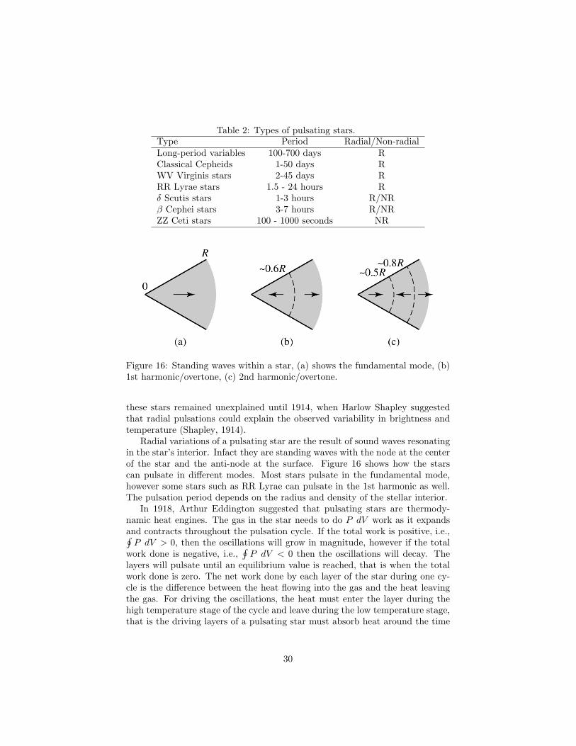
Table 2: Types of pulsating stars.Type Period Radial/Non-radialLong-period variables 100-700 days RClassical Cepheids 1-50 days RWV Virginis stars 2-45 days RRR Lyrae stars 1.5 - 24 hours Rδ Scutis stars 1-3 hours R/NRβ Cephei stars 3-7 hours R/NRZZ Ceti stars 100 - 1000 seconds NR

Figure 16: Standing waves within a star, (a) shows the fundamental mode, (b)1st harmonic/overtone, (c) 2nd harmonic/overtone.

these stars remained unexplained until 1914, when Harlow Shapley suggestedthat radial pulsations could explain the observed variability in brightness andtemperature (Shapley, 1914).

Radial variations of a pulsating star are the result of sound waves resonatingin the star’s interior. Infact they are standing waves with the node at the centerof the star and the anti-node at the surface. Figure 16 shows how the starscan pulsate in different modes. Most stars pulsate in the fundamental mode,however some stars such as RR Lyrae can pulsate in the 1st harmonic as well.The pulsation period depends on the radius and density of the stellar interior.

In 1918, Arthur Eddington suggested that pulsating stars are thermody-namic heat engines. The gas in the star needs to do P dV work as it expandsand contracts throughout the pulsation cycle. If the total work is positive, i.e.,∮

P dV > 0, then the oscillations will grow in magnitude, however if the totalwork done is negative, i.e.,

∮P dV < 0 then the oscillations will decay. The

layers will pulsate until an equilibrium value is reached, that is when the totalwork done is zero. The net work done by each layer of the star during one cy-cle is the difference between the heat flowing into the gas and the heat leavingthe gas. For driving the oscillations, the heat must enter the layer during thehigh temperature stage of the cycle and leave during the low temperature stage,that is the driving layers of a pulsating star must absorb heat around the time

30

of their maximum compression. Therefore, maximum pressure will occur aftermaximum compression and will force the gas to expand and hence causing theoscillations to amplify.

Eddington suggested that stars, the oscillations can be driven by the valvemechanism. Therefore for a star to pulsate the layer of the star needs to be-come more opaque upon compression so that the photons are trapped and as aresult heating the gas and increasing the pressure. This high pressured gas thenexpands and as it becomes more transparent, the photons can escape, allowingthe gas to cool and as a result causing the pressure to drop. The gas layerthen can fall back down due to gravity. Therefore in this model, the observedvariations correspond to the temperature change, the change in radius is has amuch smaller effect on the variations of emitted light.

In most stars the opacity increases with greater density. Remember Kramer’sopacity law (Eqn. 24):

κ = κ0ρT−3.5.

From this equation we can see that the opacity increases as the density increasesand temperature decreases. Since the opacity is more sensitive to the tempera-ture (κ ∝ T−3.5) than to the density (κ ∝ ρ) then upon compression the densityincreases and temperature also increases, and hence the opacity will decrease.This would dampen the any oscillations, and would explain why most stars donot pulsate.

The stars where the valve mechanism can operate are stars that have partialionization zones. The reason is that within layers of the star where the gasis partially ionized, part of the work done on the gas as it is compressed pro-duces further ionization rather than raising the temperature of the gas. With asmaller temperature increase, the density in Kramer’s opacity law can dominateand therefore the opacity will increase. Simalarly, when the gas expands, thetemperature does not decrease as much as expected because the ions recombinewith electrons and as a result release energy. And again the density term dom-inates, the opacity will decrease during expansion. This process is called the κmechanism.

White dwarfs with temperatures around 12 000 K have been observed to bevariable (. 0.2 magnitudes) with periods between ∼ 100 and ∼ 1000 seconds.The first variable was discovered by Arlo Landolt in 1968 (Landolt, 1968), whonoticed that the standard star HL Tau 76 was infact variable. Shortly followingthis discovery, several searches for other variable white dwarfs were conductedwith success. This led to the discovery of ZZ Ceti (Lasker & Hesser, 1971),which has become the proto-type for variable DA white dwarfs. Winget et al.(1982a) showed that the hydrogen partial ionization zone was responsible fordriving the oscillations in variable DA white dwarfs. They also predicted thatin hotter DB variable white dwarfs should also be observed where the drivingmechanism is the helium partial ionization zone. In the same year Winget et al.(1982b) reported the discovery of the variable DB white dwarf, GD 358. Sincethis discovery, several more variable DB white dwarfs have been discovered, aswell as a small number of variable DO white dwarfs (also known as PG1159

31

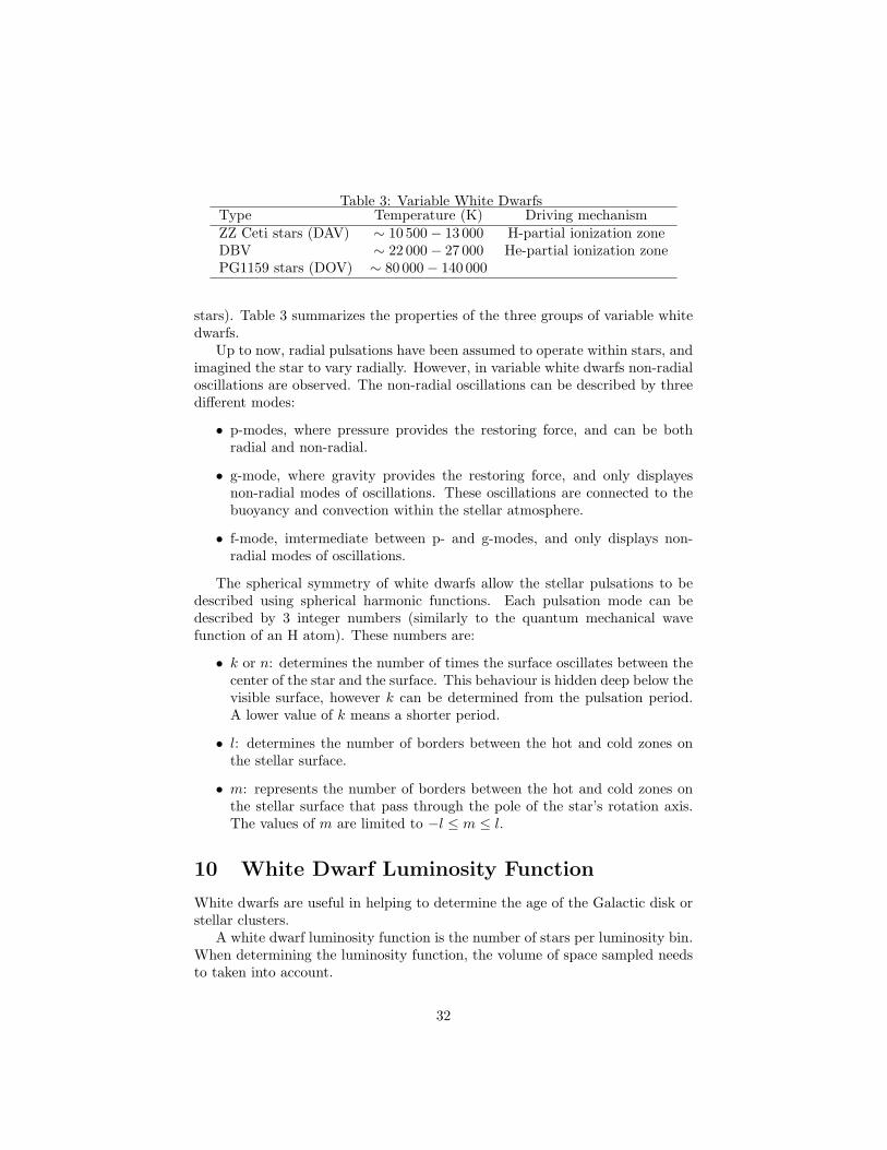
Table 3: Variable White DwarfsType Temperature (K) Driving mechanismZZ Ceti stars (DAV) ∼ 10 500− 13 000 H-partial ionization zoneDBV ∼ 22 000− 27 000 He-partial ionization zonePG1159 stars (DOV) ∼ 80 000− 140 000

stars). Table 3 summarizes the properties of the three groups of variable whitedwarfs.

Up to now, radial pulsations have been assumed to operate within stars, andimagined the star to vary radially. However, in variable white dwarfs non-radialoscillations are observed. The non-radial oscillations can be described by threedifferent modes:

• p-modes, where pressure provides the restoring force, and can be bothradial and non-radial.

• g-mode, where gravity provides the restoring force, and only displayesnon-radial modes of oscillations. These oscillations are connected to thebuoyancy and convection within the stellar atmosphere.

• f-mode, imtermediate between p- and g-modes, and only displays non-radial modes of oscillations.

The spherical symmetry of white dwarfs allow the stellar pulsations to bedescribed using spherical harmonic functions. Each pulsation mode can bedescribed by 3 integer numbers (similarly to the quantum mechanical wavefunction of an H atom). These numbers are:

• k or n: determines the number of times the surface oscillates between thecenter of the star and the surface. This behaviour is hidden deep below thevisible surface, however k can be determined from the pulsation period.A lower value of k means a shorter period.

• l: determines the number of borders between the hot and cold zones onthe stellar surface.

• m: represents the number of borders between the hot and cold zones onthe stellar surface that pass through the pole of the star’s rotation axis.The values of m are limited to −l ≤ m ≤ l.

10 White Dwarf Luminosity Function

White dwarfs are useful in helping to determine the age of the Galactic disk orstellar clusters.

A white dwarf luminosity function is the number of stars per luminosity bin.When determining the luminosity function, the volume of space sampled needsto taken into account.

32

References

Adams, W.S. 1914, PASP, 26, 198

Adams, W.S. 1915, PASP, 27, 236

Adams, W.S. 1925, Proc. N.A.S., 11, 382

Barstow, M.A., Bond, H.E., Holberg, J.B., Burleigh, M.R., Hubeny, I., &Koester, D. 2005, MNRAS, 362, 1134

Benvenuto, O.G. & Althaus, L.G. 1999, MNRAS, 303, 30

Bergeron, P., Saffer, R.A., & Liebert, J. 1992, ApJ, 394, 228

Bessel, F.W. 1844, MNRAS, 6,136

Cannon & Pickering, 1918, Harvard Annals, 92

Chandrasekhar, S. 1935, MNRAS, 95, 207

Christlieb, N., Wisotzki, L., Reimers, D., Homeier, D., Koester, D., & Heber,U. 2001, A&A, 366, 898

Eddington, A.S. 1924, MNRAS, 84, 308

Finley, D.S. & Koester, D. 1997, ApJ, 489, L79

Fowler, R.H. 1926, MNRAS, 87, 114

Giclas, H.L., Burnham Jr., R., & Thomas, N.G. 1971, Lowell Proper MotionSurvey: 8991 Northern Stars, Lowell Obs.

Giclas, H.L., Burnham Jr., R., & Thomas, N.G. 1978, Lowell Proper MotionSurvey: Southern Hemisphere Catalog, Lowell Obs. Bull. No. 164

Green, R.F., Schmidt, M., & Liebert, J. 1986, ApJS, 61, 305

Greenstein, J.L., Oke, J.B., & Shipman, H.L. 1971, ApJ, 169, 563

Holberg, J.B., Barstow, M.A., & Burleigh, M.R. 2003, ApJS, 147, 145

Kawka, A., Vennes, S., Schmidt, G.D., Wickramasinghe, D.T., & Koch, R. 2006,ApJ, 654, in press

Kilkenny, D., O’Donoghue, D., Koen, C., Stobie, R.S., & Chen, A. 1997, MN-RAS, 287, 867

Kuiper, G.P. 1941, PASP, 53, 248

Lamontagne, R., Demers, S., Wesemael, F., Fontaine, G., & Irwin, M.J. 2000,AJ, 119, 241

Landolt, A.U. 1968, ApJ, 153, 151

33

Lasker, B.M. & Hesser, J.E. 1971, ApJ, 163, L89

Leavitt, H.S. 1908, Annals of Harvard College Observatory, 60, 87

Leavitt, H.S. & Pickering, E.C. 1912, Harvard College Observatory Circulars,173, 1

Marsh, M.C., Barstow, M.A., Buckley, D.A., Burleigh, M.R., Holberg, J.B.,Koester, D., O’Donoghue, D., Penny, A.J., & Sansom, A.E. 1997, MNRAS,286, 369

Mestel, L. 1952, MNRAS, 112, 583

Russell, H.N. 1913, The Observatory, 36, 324

Russell, H.N. 1914, Nature, 93

Salim, S. & Gould, A. 2002, ApJ, 575, L83

Sion, E.M., Greenstein, J.L., Landstreet, J.D., Liebert, J., Shipman, H.L., &Wegner, G.A. 1983, ApJ, 269, 253

Shapley, H. 1914, ApJ, 40, 448

van Maanen, A. 1917, PASP, 29, 258

Vennes, S. 1999, ApJ, 525, 995

Vennes, S., Thejll, P.A., Genova-Galvan, R., & Dupuis, J. 1997, ApJ, 480, 714

Vennes, S., Thejll, P.A., Wickramasinghe, D.T., Bessell, M.S. 1996, ApJ, 467,782

Wesemael, F. 1985, QJRAS, 26, 273

Winget, D.E., Robinson, E.L., Nather, R.E., & Fontaine, G. 1982b, ApJ, 262,L11

Winget, D.E., Van Horn, H.M., Tassoul, M. Hansen, C.J., Fontaine, G., &Carroll, B.W. 1982a, ApJ, 252, L65

Wolff, B., Jordan, S., & Koester, D. 1996, A&A, 307, 149

Wood, M.A. 1995, in White Dwarfs, ed. D. Koester & K. Werner (New York:Springer), 41

34

11 Additional Reading

• Gray, D.F. The observation and analysis of stellar photospheres, 1992,Cambridge University Press

• Clayton, D.D. Principles of Stellar Evolution and Nucleosynthesis, 1983,University of Chicago Press

• Bradley, W.C. & Ostlie, D.A. An Introduction to Modern Stellar Astro-physics, 2006, Addison Wesley Publishing Company, 2nd ed.

• Rose, W.K. Advanced Stellar Astrophysics, 1998, Cambridge UniversityPress

35