whitepaper silexica LTEbasestation - Nextreamnextream.bz/file/Silexica-WhitepaperLTEBasestation.pdf · 2 LTE OVERVIEW ... 4 MAPPING ANALYSIS WITH THE SLX TOOL SUITE ... and parameter

1

© 2016 Silexica GmbH. All rights reserved worldwide.

WHITEPAPER

USING THE SLX TOOL SUITE FOR MULTICORE SOFTWARE DESIGN OF AN LTE BASE STATION


Table of Contents

1 INTRODUCTION ............................................................................................................................................................. 3

2 LTE OVERVIEW .............................................................................................................................................................. 3 2.1 LTE FRAME ................................................................................................................................................................. 3 2.2 PHYSICAL CHANNELS ............................................................................................................................................... 4 2.2.1 PBCH (PHYSICAL BROADCAST CHANNEL) .................................................................................................. 4 2.2.2 PCFICH (PHYSICAL CONTROL FORMAT INDICATOR CHANNEL) .......................................................... 5 2.2.3 PDCCH (PHYSICAL DOWNLINK CONTROL CHANNEL) ............................................................................. 5 2.2.4 PHICH (PHYSICAL HYBRID-ARQ INDICATOR CHANNEL) ........................................................................ 5 2.2.5 PDSCH (PHYSICAL DOWNLINK SHARED CHANNEL) ................................................................................ 5

3 APPLICATION OVERVIEW ....................................................................................................................................... 5 3.1 PARALLELIZATION STRATEGY ............................................................................................................................... 6

4 MAPPING ANALYSIS WITH THE SLX TOOL SUITE .................................................................................. 7 4.1 GENERIC BASEBAND PROCESSING MULTI-DSP PLATFORM ...................................................................... 8 4.2 GENERIC DSP ARCHITECTURE ENHANCED WITH HARDWARE ACCELERATORS .............................. 13 4.3 EXPLORING DIFFERENT PROCESSOR FREQUENCIES AND POWER ANALYSIS .................................. 17

5 CONCLUSION ............................................................................................................................................................... 19


1 Introduction

This paper presents a typical base station design scenario, where decisions about HW/SW partitioning, the number of processing elements, and operational system parameters, among other things, need to be made early on by system architects. The SLX Tool Suite determines the impact of these various design decisions and parameter selections, while exploring different target architecture configurations and checks if application constraints can be met. In the following, an LTE DownLink Application is used as the application driver.

2 LTE Overview

LTE (Long Term Evolution), also known as E-UTRAN (Evolved Universal Terrestrial Access Network), introduced in 3GPP R8, is the access part of the Evolved Packet System (EPS). The main requirements for the new access network are high spectral efficiency, high peak data rates, short round-trip time as well as flexibility in frequency and bandwidth. The case tested here is the implementation of the DownLink (DL) Physical Layer (PHY) of an LTE eNodeB (base station). The LTE PHY specification accommodates bandwidths from 1.25MHz to 20MHz. Orthogonal frequency division multiplexing (OFDM) is the selected modulation. The DL is composed of physical channels that convey information from the higher layer and some synchronization signals. Here, we consider the following channels and signals:

PBCH: Physical Broadcast Channel, PCFICH: Physical Control Format Indicator Channel, PHICH: Physical Hybrid-ARQ Indicator Channel, PDSCH: Physical Downlink Shared Channel, PDCCH: Physical Downlink Control Channel, P-SS: Primary Synchronization Signal, S-SS: Secondary Synchronization Signaling.

2.1 LTE Frame

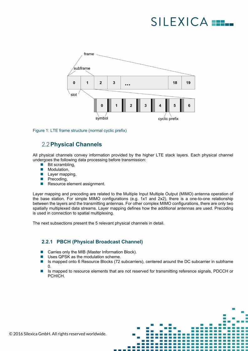
LTE frames are each 10 ms in duration. They are divided into 10 subframes, with each subframe duration being 1 ms. Each subframe is further divided into two slots of 0.5 ms each. Slots consist of either 7 or 6 OFDM symbols, depending on whether the “normal” or “extended” cyclic prefix is being employed. A symbol corresponds to a certain time span of a signal, carrying one spot in the modulation schemes I/Q- Constellation Diagram. Figure 1 shows the structure of a frame. In OFDMA (Orthogonal Frequency Division Multiple Access), a specific number of subcarriers for a determined amount of time are allocated to the users. These are referred to as Physical Resource Blocks (PRBs). PRB allocations are handled by higher protocol layers in the eNodeB. The available number of PRBs is determined by the bandwidth of the transmission (e.g. 100 PRBs in 20 MHz).


Figure 1: LTE frame structure (normal cyclic prefix)

2.2 Physical Channels

All physical channels convey information provided by the higher LTE stack layers. Each physical channel undergoes the following data processing before transmission:

Bit scrambling, Modulation, Layer mapping, Precoding, Resource element assignment.

Layer mapping and precoding are related to the Multiple Input Multiple Output (MIMO) antenna operation of the base station. For simple MIMO configurations (e.g. 1x1 and 2x2), there is a one-to-one relationship between the layers and the transmitting antennas. For other complex MIMO configurations, there are only two spatially multiplexed data streams. Layer mapping defines how the additional antennas are used. Precoding is used in connection to spatial multiplexing. The next subsections present the 5 relevant physical channels in detail.

2.2.1 PBCH (Physical Broadcast Channel)

Carries only the MIB (Master Information Block). Uses QPSK as the modulation scheme. Is mapped onto 6 Resource Blocks (72 subcarriers), centered around the DC subcarrier in subframe

0. Is mapped to resource elements that are not reserved for transmitting reference signals, PDCCH or

PCHICH.


2.2.2 PCFICH (Physical Control Format Indicator Channel)

Carries the number of symbols that can be used for control channels (PDCCH and PHICH). Mapped onto the first OFDM symbol in each downlink subframe, occupying 16 data subcarriers of the

symbol. User equipment (UE) decodes this channel to figure out how many OFDM symbols are assigned for

the control channels (PDCCH and PHICH). The exact position of PCFICH is determined by cell ID and bandwidth.

2.2.3 PDCCH (Physical Downlink Control Channel)

Mapped to the first OFDM symbol in each downlink subframe. Number of symbols used for PDCCH: can be 1, 2, or 3. Number of symbols used for PDCCH is specified by PCFICH. PDCCH carries downlink control information (DCIs). Multiple PDCCHs can be assigned in a single subframe. UE then does blind decoding of all PDCCHs. Uses QPSK as the modulation scheme.

2.2.4 PHICH (Physical Hybrid-ARQ Indicator Channel)

Carries repeat request (H-ARQ) feedback for the received PUSCH. Depending on the configuration, several PHICHs constitute a PHICH group using the same resource

elements.

2.2.5 PDSCH (Physical Downlink Shared Channel)

Carries user-specific data (DL Payload). Carries random access response message. Uses Adaptation Modulation and Coding (AMC) with QPSK, QAM16, QAM64 or QAM256 modulation

schemes. This actual modulation scheme is determined by the modulation and coding scheme (MCS) carried within the DCI specified by PDCCH.

3 Application Overview

The application under analysis implements the DL transmission procedure performed by an LTE eNodeB. It constructs a test FDD subframe and transmits it. The application performs all corresponding physical layer (PHY) tasks necessary for encoding, modulating and transmitting the PBCH, PDSCH, PHICH, PDCCH and PCFICH physical channels. Since an LTE subframe transmission duration is equal to 1 ms, all prior processing must fulfill a very tight latency constraint (tl). In order to fulfill tl the processing for the subframe must take at most 1 ms (excluding some initial base station setup time). If the processing time is greater than tl then the next subframe will not be ready when the previous subframe completes transmission. Our application is implemented as a data flow model containing 73 processing tasks of varying complexity. Tasks communicate with other tasks via first-in first-out (FIFO) channels, which are initially unmapped to platform communication means. That is, all channels are treated in an abstract manner without defining whether they are mapped onto shared memories, for instance, or handled via DMAs (Direct Memory Access devices). Overall, there are 186 inter-task communication channels. Figure 2 presents the graphical view of


an application fragment as shown by the Silexica Tool Suite. Tasks implementing LTE physical channels and the data flow amongst them can be observed.

Figure 2: LTE application diagram in the SLX Tool Suite

3.1 Parallelization Strategy

The application follows a coarse-grain parallelization strategy that exploits mostly Task-Level Parallelism (TLP) and Pipeline-Level Parallelism (PLP). There is one parallel pipeline for each channel flow, where the specific channel data is processed. When the channel data is encoded, it enters a parallel processing flow that is replicated according to the number of antennas in the system. Figure 3 shows a high-level overview of the parallelism exploited in the application.


Figure 3: Parallelism exploited in application

In order to better understand the concept of a channel pipeline, consider the PDSCH pipeline shown in Figure 4. A controller task called PDSCH_ctrl (1) drives the entire channel flow after receiving encoding parameters and input data from higher layers. The PDSCH_cb task (2) segments the input data into code blocks for encoding. The PDSCH_cb_encod task (3) performs turbo coding and rate matching on the code blocks. The PDSCH_concat task (4) concatenates the resulting encoded code blocks, which are later scrambled by the PDSCH_scrambler task (5). Afterwards, the PDSCH_modmapper (6) performs the channel-specific modulation mapping, which results in a stream of modulation symbols that have to be mapped to layers (PDSCH_lmapper - 7) and precoded (PDSCH_precoder - 8) before transmission (depending on the current transmit diversity and spatial multiplexing settings).

Figure 4: Channel pipeline example

4 Mapping Analysis with the SLX Tool Suite

In the following, we use the Silexica Tool Suite to map the application tasks to processing elements for different target architectures. The SLX Mapper has built-in Mapping and Scheduling algorithms that can find high performance mappings for different optimization goals, such as power, load, and execution time. This determines whether the required application constraints are met when mapping an application to a specific target architecture. With the SLX Explorer, varying combinations of system parameters, such as the number of processors, memory sizes, and processor frequency, among others, can be evaluated automatically. This way, the SLX Mapper and SLX Explorer help to answer critical design questions and to perform power/cost/performance trade-off experiments at early design stages.


The LTE test application will be analyzed with the following platforms: A generic baseband processing multi-DSP architecture with 16 TI C66x DSP cores operating at 1 GHz An enhanced version of the generic baseband processing multi-DSP architecture including 6 hardware

accelerators These architectures represent the baseband processing systems typically used today by most wireless providers. It is also worth mentioning that application mapping/distribution analyses for off-the-shelf System on Chips (SoCs) can also be performed with the SLX Mapper in the same way as for these generic architectures, but this is out of the scope of this paper.

4.1 Generic Baseband Processing Multi-DSP Platform

We compute multiple automatic mappings for the application on the generic baseband processing multi-DSP platform by considering subsets of cores of increasing size. This way the optimal platform size for an application can be estimated. We computed automatic mappings when using 1, 2, 4, 6, 8, 10, 12, 14 and 16 cores in the platform. Figure 5 presents the Mapping Analysis Results Chart generated by the SLX Mapper. The mapping strategy used in these experiments tries to achieve load and data throughput balancing across the system. The Mapping Analysis Results Chart helps keep track of the performance of different configurations.

Figure 5: Mapping Analysis Results for up to 16 cores on Generic Baseband Processing Multi-DSP Platform

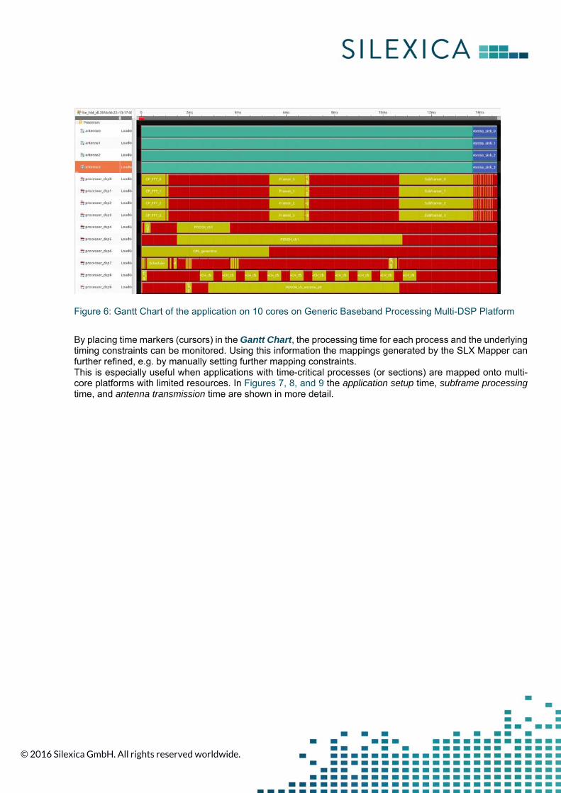
For the evaluated LTE application, increasing the number of cores consistently decreases the execution time. However, after a certain number of cores are used in the platform, adding more cores only produces marginal improvements. The spatial and temporal mapping (scheduling) computed by the SLX Mapper can be seen in the Gantt Chart in Figure 6.


Figure 6: Gantt Chart of the application on 10 cores on Generic Baseband Processing Multi-DSP Platform

By placing time markers (cursors) in the Gantt Chart, the processing time for each process and the underlying timing constraints can be monitored. Using this information the mappings generated by the SLX Mapper can further refined, e.g. by manually setting further mapping constraints. This is especially useful when applications with time-critical processes (or sections) are mapped onto multi-core platforms with limited resources. In Figures 7, 8, and 9 the application setup time, subframe processing time, and antenna transmission time are shown in more detail.


Figure 7: The application setup time highlighted in the Gantt Chart


Figure 8: The application subframe processing time highlighted in the Gantt Chart

Figure 9: Antenna transmission time highlighted in the Gantt Chart

The scheduling state (ready, running, read-blocked, write-blocked) over time for each process can be seen in the Task State Graph, which allows users to easily spot bottlenecks associated with read or write-blocks. Figure 10 shows the Task State Graph for the 10-core mapping.


Figure 10: Task State Graph

Even with 16 cores, the best execution time we were able to achieve was 13.95 ms. This is not even close to being acceptable for a base station configuration. Using the Profiler view, one can check the process execution time for all application tasks on all processor types in the platform, as shown in Figure 11. In the figure, the reported times are for the TI 66x DSP core running at 1 GHz. It can be seen that the processes that take the most time are the FFT/IFFTs, turbo coding and bit-level processing tasks in the PDSCH channel.


Figure 11: Estimated process execution times for each process

4.2 Generic DSP Architecture Enhanced with Hardware Accelerators

After identifying the most time/cycle-consuming processes, we off-loaded them to hardware accelerators to see how this changes the application execution time. The enhanced architecture comprises 6 additional hardware accelerators: 4 for FFT/IFFT computation, one for turbo encoding and one for PDSCH bit-code processing. Additionally, we now add to the application specification a real-time latency constraint that specifies the processing time required for a subframe. The most important constraint in LTE is that a subframe is encoded within 1 ms so as to allow the uninterrupted transmission of subsequent subframes. Transmission itself takes an additional 1 ms, but it is performed only by the antennas when the channel data has already been prepared. Therefore, task mapping decisions have significant influence on the first 1 ms (processing time) for a subframe, but no influence at all on the actual transmission time. Apart from the 2 ms subframe time mentioned above (i.e. 1 ms for processing, 1 ms for transmission), a certain initial setup time must be accounted for when booting the system up and preparing the first frames and subframes. During this time, processes like computing the user RB scheduling (performed in higher layers), encoding unique cell identifiers and preparing synchronization signals for the rest of a transmission scenario take place. When these are added together, our selected subframe time constraint is 2.6 ms, corresponding to 1.6 ms for setup and processing and 1 ms for transmission. Specifying a constraint causes the SLX Mapper to automatically try to find the best system configuration to fulfill it. It is worth mentioning that, although the SLX Tool Suite uses cross-target performance estimation tools that can guess the execution time of tasks on processors and DSPs, adding HW accelerators to the system requires the user to provide manual timing annotations for the affected tasks. This is a straightforward procedure, as only a couple of lines have to be added into the application source code. The actual timing numbers come from data sheets, existing implementations or from the user’s experience.


Similar to previous experiments, the system is analyzed after gradually increasing the number of cores until the imposed timing constraint is met. Figure 12 shows the Mapping Analysis Result comparison for 4 and 6 cores with our previous generic baseband processing multi-DSP architecture.

Figure 12: Mapping Analysis Result comparison for 4 and 6 cores

A significant improvement in the execution time can be seen with the enhanced platform. Offloading the highly time-consuming processes decreases execution time by up to 7x and improves performance by 85%. Although the constraint is not met using the enhanced platform with 4 cores, the application setup time and subframe processing time are significantly reduced when compared to the results for the previous architecture (see Figures 7 and 8). Figures 13, 14 and 15 show the respective Gantt charts for 4 cores with hardware accelerators.


Figure 13: Gantt chart for 4 cores and hardware accelerators

Figure 14: Gantt chart for application setup time


Figure 15: Gantt chart for subframe processing time

From the figures, the subframe setup and processing time is 1.25 ms + 0.78 ms = 2.03 ms. This, added to the 1 ms time required for transmission, still does not fulfill the selected constraint of 2.6 ms. As the current architecture possesses additional DSP cores, one can continue mapping the application onto more cores to see the effect. Figure 16 shows the Mapping Analysis Results Chart for 1, 2, 4, 6, 8, 10, 12 and 14 DSP cores and the 6 hardware accelerators.

Figure 16: Mapping result for up to 14 cores on generic DSP architecture with hardware accelerators


This time, one can see that using 10 or more DSP cores fulfills the 2.6 ms constraint. The final decision about whether a platform with 10, 12 or 14 cores will be used needs to come after a cost-benefit analysis performed by the system architects. As a matter of fact, faster execution times would certainly leave room to add other tasks later, for instance (e.g. protocol improvements), but this would also yield a higher SoC area that could affect the design’s cost effectiveness.

4.3 Exploring Different Processor Frequencies and Power Analysis

At this point, many other questions can be easily answered by using the SLX tools. For instance, can the number of cores further be reduced by increasing the processor, bus and memory frequencies? To demonstrate how to answer these questions, we focus next on the cases for 4 and 10 cores, which yielded execution times of 3.04 ms and 2.51 ms respectively. This corresponds to an execution time difference of about 18%. By quickly modifying the SLX high-level architecture model, we increased the frequency of all DSPs from 1 GHz to 1.3 GHz, and mapped the application again on only 4 cores. The Mapping Analysis Results Chart in Figure 17 shows the comparison between 10 cores operating at 1 GHz and 4 cores operating at 1.3 GHz.

Figure 17: Mapping analysis result for cores with different operating frequencies

As can be seen, mapping onto 4 cores running at 1.3 GHz yields a significantly better execution time than using 10 cores at 1 GHz. Once again, these results and subsequent cost-benefit analyses can help system architects make critical early design decisions. So far, increasing the operating frequency may sound like a sure-fire way to improve the overall execution time of the application. However, it might also have several implications for the power consumed by the base station. For instance, peak power plays an important role in the design of base stations, as power sources in deployed antenna sites are usually constrained. By relying on system-level power estimation strategies, the SLX Mapper can also provide Power Profile Charts that help to analyze this dimension of the system. Figure 18 shows the resulting Power Profile chart after mapping and scheduling of the application on 4 cores at 1GHz.


The figure depicts how much total and individual power/energy is consumed by each core and at which points in time. This allows the user to spot, for instance, critical application sections where an allowed maximum peak power is overshot. The power analysis features in the SLX Mapper are enabled by providing switching capacitance values of processors’ functional units, memories and buses, and by specifying the system’s voltage and frequency domains/settings.

Figure 18: Power Profile chart

Comparing now the power profile chart of the mapping scenario for 4 cores at 1.3 GHz vs. 10 cores at 1.0 GHz, one can find which system yields better power efficiency. Figures 19 and 20 show fragments of the Power Profile charts of these two mapping configurations.

Figure 19: Power Profile chart for 4 cores @ 1.3 GHz operating frequency

Figure 20: Power Profile chart for 10 cores @ 1 GHz operating frequency


In this case, it can be seen that mapping the application onto only 4 cores at 1.3 GHz does cause a peak power increment of 15% compared to the case of 10 cores at 1 GHz. However, computing the system’s power efficiency in terms of subframes per Watt-second with the formula

∗

shows that the solution with 4 cores at higher frequency is superior, resulting in a 13% gain.

5 Conclusion

In this report we took a complex LTE base station application and mapped it onto two different architectures, using Silexica Tools. Not only did we map and run the application onto these architectures, but we also experimented with different hardware configurations to determine whether different constraints are met (i.e. peak power and total execution time). All in all, Silexica Tools provide system architects with detailed insights into their target multicore system, and facilitate quick HW/SW partitioning, mapping and scheduling analyses that help system architects answer early design questions and allow them to make informed design decisions early on in the design process.

Documents

whitepaper silexica LTEbasestation - Nextreamnextream.bz/file/Silexica-WhitepaperLTEBasestation.pdf · 2 LTE OVERVIEW ... 4 MAPPING ANALYSIS WITH THE SLX TOOL SUITE ... and parameter