Who Bears the Burden of Energy Taxes?

The Role of Local Pass-Through

Samuel Stolper∗

October 25, 2016

Abstract

Existing estimates of energy tax incidence assume that the pass-through of taxes to final con-

sumer prices is uniform across the affected population. I show that, in fact, variation in local

market conditions drives significant heterogeneity in pass-through, and ignoring this can lead to

mistaken conclusions about the distributional impacts of energy taxes. I use data from the Spanish

retail automotive fuel market to estimate station-specific pass-through, focusing on the effects of

competition and wealth. A novel informational mandate provides access to a national, station-daily

panel of retail diesel prices and characteristics and allows me to investigate market composition at a

fine level. Event study and difference-in-differences regression reveal that, while retail prices rise

nearly one-for-one (100%) with taxes on average, station-specific pass-through rates range from at

least 70% to 120%. Greater market power – measured by brand concentration and spatial isolation –

is strongly associated with higher pass-through, even after conditioning on detailed demand-side

characteristics. Furthermore, pass-through rises monotonically in area-average house prices. While

a conventional estimate of the Spanish diesel tax burden suggests roughly equivalent incidence

across the wealth distribution, overlaying the effect of heterogeneous pass-through reveals the tax to

be unambiguously progressive.

Keywords: Incidence, Pass-Through, Energy, Market Power

JEL Codes: H22, L13, Q41

∗MIT (email: sstolper@mit.edu). I would like to thank Joseph Aldy, Nathan Hendren, Erich Muehlegger, Robert Stavins,and Jim Stock for invaluable guidance and support. I also thank Todd Gerarden, Richard Sweeney, Evan Herrnstadt, BenjaminFiegenberg, Yusuf Neggers, Eric Dodge, Harold Stolper, and Katie Rae Mulvey for helpful comments and discussion, as well asseminar participants at Harvard University. I am especially grateful to Manuel Garcia Hernández, Sergio López Pérez, CarlosRedondo López, and colleagues at the Spanish Ministry of Energy and the National Commission on Markets and Competitionfor generously providing me with access to the Geoportal data, as well as a greater understand of Spain’s oil markets.

1

1 Introduction

Energy taxes – and related market-based policies – are attractive because they have the potential

to reduce negative externalities like pollution, traffic, and accident risk in a cost-effective manner,

thereby raising social welfare. But what are the distributional impacts of these policies? Researchers

(Morris and Munnings 2013), politicians (Metcalf, Mathur, and Hassett 2011), and popular media

(New York Times 2009) alike have long debated the economic incidence of energy taxes - for example,

how much of the tax burden is borne by consumers versus suppliers, and how taxes affect households

of different wealth levels. Distributional outcomes are increasingly subject to scrutiny as the demand

for climate policy grows, and as the scope and scale of household energy use continue to increase.

In this paper, I provide new insight into distributional questions about energy policy by estimating

the pass-through of automotive fuel taxes to final, retail prices. Pass-through – the degree to which

costs physically imposed on one segment of a market are “passed through” to others – is a useful

economic tool for at least two reasons. First, it is determined in equilibrium by supply, demand, and

competition; thus, empirical pass-through patterns provide indirect insight into underlying market

function. Second, pass-through measures the extra cost of maintaining consumption in the face of a

tax hike, thereby providing direct insight into tax incidence. I make use of these attributes by studying

how energy tax pass-through rates vary with local competition and consumer characteristics.

My focus is on the retail automotive fuel market of Spain, whose government provides access to

daily gas-station prices and characteristics through a novel informational mandate issued in 2007.

State-specific taxes on automotive fuel provide panel variation in tax levels. Cross-sectional variation

in branding and location, as well as temporal variation in local competition generated by entry and

exit of stations, allows me to estimate a relationship between tax pass-through and market power.

Survey measures of population, property values, and education aid in the identification of that

relationship and also facilitate a study of the relationship between pass-through and wealth.

I find that branding and location patterns in the Spanish market predict significant heterogeneity in

pass-through. Moreover, pass-through exhibits a strong positive correlation with wealth, as measued

by local house prices. These results challenge the wisdom of existing energy tax incidence analyses

(e.g., West 2004; Bento et al. 2009; Grainger and Kolstad 2010), which consistently find that taxes on

gasoline and carbon dioxide are regressive – i.e., relatively worse for poorer people than for richer

ones – in industrialized countries. These analyses focus primarily on how differences in consumption

(both before and after a tax change) across the wealth spectrum affect distributional equity, but they

2

assume away corresponding differences in prices. My own analysis suggests that the price impacts of

taxation (measured by pass-through) are not only non-uniform, but also systematically related to

wealth. When I account for this in my own incidence calculation, the Spanish tax appears strongly

progressive.

My empirical analysis is essentially a comparison of prices before and after tax hikes, at stations

of different types. I begin with an event study of tax hikes, which provides a sense of price trends

at stations experiencing tax hikes relative to those not experiencing them. The results imply that

“treatment” and “control” stations have parallel price trends before and after tax events. Motivated

by this finding, I use difference-in-differences (DiD) regression to estimate an average pass-through

rate of 95% for Spanish diesel taxes (diesel is the dominant automotive fuel in Spain). However,

this average rate masks significant heterogeneity at the local level. I capture this heterogeneity by

comparing prices before and after taxes among stations with (a) different brands, (b) facing different

numbers and types of rivals, and (c) serving different consumer bases. Econometrically, I do this by

re-estimating event study and DiD models while interacting my tax variable with characteristics of

stations and their surroundings.

The results show that stations bearing the brand of a vertically-integrated refiner are associated

with significantly higher tax pass-through, as are stations facing relatively less-dense spatial compe-

tition. In addition, pass-through rises in the local concentration of one’s own brand. While brand

and location are likely endogenous due to station owners’ consideration of local demand in their

decisions, the inclusion of a suite of detailed demand-side characteristics in regression analysis leaves

my main estimates unchanged. Through both a branding channel and a spatial channel, market

power appears to raise pass-through.

I also find that pass-through rises monotonically in area-average house prices. I cannot interpret

this relationship as causal, but it is nonetheless the case that richer areas see, on average, higher price

impacts of taxation, even conditional on local market structure. Together, competitive environment

and local consumer characteristics predict a wide distribution of pass-through rates among Spanish

gas stations, centered around 90% but ranging from approximately 70 to 115%. The existence of

overfull (>100%) pass-through may seem surprising, but it has been found in other markets (Besley

and Rosen 1999) and is the natural result of imperfect competition with sufficiently convex demand

(Seade 1985). In Spain, 24% of gas stations have estimated pass-through rates in excess of 100% on

the last day of observation in my sample period.

3

The combination of imperfect competition and convex demand has significant implications for

tax incidence. Perfect competition, which is a standard assumption in energy tax incidence analysis,

bounds pass-through between 0 and 100%; since empirical research shows that fuel tax pass-through is

nearly 100% on average (see, e.g., Marion and Muehlegger 2011), the perfect-competition assumption

implies 100% pass-through everywhere. This uniform, full pass-through rate is what is applied

in nearly every incidence analysis to date. My results, in contrast, show that pass-through varies

substantially across space.

Pass-through variation intimately affects distributional equity, by imposing larger price impacts

on richer areas. Existing incidence analyses miss this effect by using a uniform pass-through rate. To

show the consequences of this omission, I estimate the effect of a marginal tax hike on household tax

burdens, before and after accounting for the relationship between pass-through and wealth. I obtain

annual automotive fuel consumption totals for a sample of households from the Spanish Household

Budget Survey. This quantity, multiplied by the pass-through rate, and divided by total household

expenditure, gives an estimate of the marginal tax burden as a proportion of wealth. Existing analyses

of this type assume a pass-through rate of 100%; replicating this assumption yields burden estimates

that are roughly equivalent across wealth deciles. In contrast, using estimated pass-through rates

specific to each house-price decile yields burden estimates that rise with wealth.

The conventional wisdom is that gasoline and diesel taxes are regressive in industrialized countries

because the poor in those countries tend to spend a larger proportion of their wealth on energy than

the rich. This presents a serious, oft-cited flaw in a policy instrument that is generally seen as good for

overall social welfare. But it relies in part on an assumption of uniform pass-through that I here prove

inaccurate. All else equal, a positive relationship between pass-through and wealth makes taxes more

progressive. In Spain, it turns a tax with roughly flat incidence across the wealth distribution into

a progressive policy. To the extent that the positive relationship between pass-through and wealth

holds in other contexts, taxes on those energy products and in those locales become correspondingly

more attractive from a distributional standpoint. More generally, the widespread heterogeneity that

I identify due to variation in local competition and preferences suggests that analysts should not

assume away cross-sectional differences in the price impacts of energy regulation. Reduced-form

pass-through estimation provides a tractable way of addressing this problem.

The rest of this paper is laid out as follows: Section 2 describes what is known, in theory and in

empirics, about energy tax incidence; Section 3 provides a picture of the Spanish automotive fuel

4

market and the relevant taxes and data; Section 4 describes my analysis of average tax pass-through;

Section 5 details the corresponding estimation of local tax pass-through as a function of market

structure and consumer makeup; Section 6 discusses the distributional implications of these results;

and Section 7 concludes.

2 Pass-Through in the Existing Literature

The term “pass-through” refers to what Alfred Marshall (1890) described as “the diffusion throughout

the community of economic changes which primarily affect some particular branch of production

or consumption.” Most commonly, these “economic changes” are costs, physically imposed on one

part of a supply chain, and passed through to others. As Weyl and Fabinger (2013) have recently

highlighted, pass-through has extraordinary potential as a tool of economic analysis. For this reason,

several disciplines of economics feature the topic in research. International economists have long been

concerned with exchange-rate pass-through, because of its role in explaining movements in relative

prices and business cycles (Auer and Schoenle 2013). The field of industrial organization contains

much research on pass-through because of the light it sheds on mergers (Jaffe and Weyl 2013) and

price discrimination (Aguirre, Cowan, and Vickers 2010). In public finance, pass-through is important

primarily because of its connection to tax incidence. This last application is the one on which I focus.

2.1 The use of pass-through in incidence analysis

The change in consumer surplus elicited by a rise in energy taxes is naturally divided into two

components: (a) the additional cost of energy consumption maintained in the face of rising prices;

and (b) the utility lost from reduced consumption (i.e., the deadweight loss).1 Pass-through physi-

cally measures the former, per unit consumption. It is thus an integral part of incidence analysis,

which generally focuses on estimating changes in surplus among different segments of society (e.g.,

consumers vs. producers, and richer vs. poorer). If the price impacts of rising taxes vary across

geographic regions, firms, or individuals, then distributional welfare will vary accordingly.

Existing analyses of energy tax incidence, however, assume without exception that pass-through

of taxes – whether on gasoline (West 2003; West and Williams 2004; Bento et al. 2005, 2009) or on

1Consumer surplus is also determined by (a) ownership of supply-side capital; (b) externalities like pollution, traffic, andvehicular safety; (c) other goods’ prices that are affected by energy taxes in general equilibrium; and (d) the use of governmentrevenues obtained through taxation. In this paper, however, I focus only on the utility derived directly from the purchase andconsumption of energy. See Sterner (2012) for a fuller discussion of the various channels through which a tax affects welfare.

5

carbon (Metcalf 2009; Grainger and Kolstad 2010; Metcalf, Mathur, and Hasset 2011; Mathur and

Morris 2012) – is uniform across the affected population. With one exception (Metcalf, Mathur, and

Hasset 2011), these analyses further assume that pass-through is fully 100% (one for one).

Why is pass-through assumed or expected to be uniformly 100%? The answer is a combination

of theory, intuition, and empirics. The natural starting point in public finance is of tax incidence in

perfect competition. In such a model, pass-through is entirely a function of the elasticities of supply

and demand. Equation 1 provides the mathematical definition (see Appendix A for the derivation):

dpc

dt=

εSεS − εD

=1

1− εDεS

(1)

Pass-through of tax t to retail price pc rises in the supply elasticity (εS) and falls in the absolute

demand elasticity (εD). In the polar cases of either perfectly elastic supply (εS → +∞) or perfectly

inelastic demand (εD → 0), pass-through rates are identically 100%.

The consensus intuition about automotive fuel markets is that retail supply is very elastic –

because of opportunities for storage and the ease of purchasing wholesale fuel for resale – and that

retail demand is very inelastic – because driving is a fundamental input to so many daily activities.

Empirical research suggests that at least the latter is true (Dahl 2012; Hughes, Knittel, and Sperling

2008). In perfect competition, the expected result is thus high (i.e., close to 100%) pass-through.

The empirical pass-through literature strongly supports the above intuition: estimated average

pass-through rates in automotive fuel markets are consistently 100% or very nearly so (Alm, Sennoga,

and Skidmore 2009; Marion and Muehlegger 2011; Bello and Contín-Pilart 2012). High pass-through

has also been found for the cost of permits under the European Union Emissions Trading System

(Fabra and Reguant 2014) and credits (“RINs”) under the U.S. Renewable Fuel Standard (Knittel,

Meiselman, and Stock 2015). Pass-through is bounded above by 100% in perfect competition, as

can be seen from Equation 1; in such a model, full pass-through on average therefore implies full

pass-through everywhere. This, perhaps, is why researchers assume the latter in incidence analysis.

2.2 The logic of heterogeneous pass-through

Once the assumption of perfect competition is set aside, full pass-through on average no longer

guarantees full pass-through locally. In imperfect competition, pass-through varies with not just the

6

first derivative (elasticity), but also the second (convexity). Consider the formula for pass-through in

monopoly with constant marginal costs c:

dpm

dt=

∂p(qm)∂qm

2 ∂p(qm)∂qm

+ qm∂2 p(qm)

∂q2m

(2)

The shape of demand – described by ∂p(qm)∂qm

and ∂2 p(qm)

∂q2m

– is integral to the magnitude of monopoly

pass-through. In oligopoly, the same holds true: tax pass-through depends on first and second

derivatives of demand with respect to both one’s own prices and the prices of its competitors (again,

see Appendix A for the derivation of pass-through in imperfect competition).

Anything that affects the shape of demand causes a change in the level of pass-through. For

example, greater market power at some gas station i, due to either larger market shares or greater

spatial isolation, could reduce the magnitude of ∂q(pi)∂pi

; this would, in turn, lead to a different pass-

through rate than at other stations. Along these lines, Doyle and Samphantharak (2008) find that

pass-through of U.S. sales taxes into retail gasoline prices is lowest in areas with the lowest brand

concentration.2 At the same time, consumer preferences or budget constraints could also affect the

shape of demand. Though the direct relationship between pass-through and wealth is undocumented,

it is nonetheless clear that demand could be more or less elastic in richer areas, relative to poorer

ones. Such variation would, in turn, drive differences in pass-through.3

One important observation from Equation 2 is that the sign of the relationship between pass-

through and (absolute) demand elasticity is theoretically ambiguous. If demand is linear, the second

derivative of demand is zero, and monopoly pass-through collapses to 50% regardless of the slope of

demand. If demand is concave, then pass-through is below 50%, and more inelastic demand leads to

lower pass-through, all else equal. If demand is convex, then pass-through is above 50%, and more

inelastic demand leads to higher pass-through, all else equal. With prior knowledge of the second

derivative of demand, this ambiguity is resolved. Without it, the relationship between market power

and pass-through, or wealth and pass-through, becomes an empirical question.

2Miller, Osborne, and Sheu (2015) investigate the effect of spatial isolation on fuel cost pass-through in the U.S. cementmarket. They find that increasing distance to competitors raises own-cost pass-through but reduces rival-cost pass-through; thetwo channels cancel each other out, so that pass-through is empirically insensitive to spatial competition.

3The shape of the supply curve is similarly relevant, though I assume it to be flat in Equation 2. Marion and Muehlegger(2011) identify a positive relationship between tax pass-through and the elasticity of supply in retail automotive fuel markets.

7

2.3 Overfull pass-through

In certain circumstances, pass-through can even exceed 100% (Seade 1985). To see this point, consider

the graphical depiction of (excise) tax pass-through in Figure 1. The two panels denote identical

settings of linear supply, isoelastic demand, and a tax hike dt that shifts supply upwards from S0 to

S1. (P1 − P0) is thus the change in price due to the tax hike. There is only one difference between

the two panels: in Panel A, competition is perfect, while in Panel B, supply is a monopoly. Panel A

prices are simply set at the intersection of D and S. Panel B prices, in contrast, are set according to

the marginal revenue curve MR. The monopolist first finds its optimal quantity at the intersection of

MR and D, and then maps this quantity back to price using the demand curve.

Pass-through in Panel A is 100% because supply is perfectly elastic (i.e., flat); in Panel B, however,

pass-through is greater than 100% (dp > dt). This “overfull” pass-through is a result of the interaction

between market power and sufficiently convex demand. Market power shifts the relevant quantity

range, and demand convexity causes the slope of demand to be steeper over this new range. The

slope is so steep that the resulting jump in prices exceeds the rise in taxes.

Overfull pass-through has been found in a variety of markets (see, e.g., Besley and Rosen 1999),

but in automotive fuel markets it has only been found in certain situations of abnormally high supply

elasticity (Marion and Muehlegger 2011). To the extent that overfull pass-through is observed in

energy markets, one plausible explanation is differential consumer search. If a fraction of consumers

in a market are price-insensitive and always patronize the same gas station, while a fraction shop

around much more, then demand may have the required convex shape. More generally, demand

could be convex if those with the highest willingness to pay for energy are relatively richer, and if

richer individuals are less price-sensitive than poorer ones. This latter pattern is a common result

estimated in structural models of demand for a variety of goods (including, most relevantly, Houde

2012 for retail gasoline).

The preceding discussion serves to highlight the divergence between energy tax incidence analysis

and its theoretical foundations. Pass-through need not be exactly 100%, and it can vary substantially

at a local level due to the shape of demand and supply and the toughness of competition. In the next

section, I introduce the data that I use to identify this local pass-through.

8

3 Background on Spain’s Oil Markets

The Spanish retail automotive fuel market is an ideal setting for a study of the determinants of energy

tax incidence: it appears highly imperfectly competitive;4 it features panel variation in state-level

taxes; and the government records very detailed price data in it. Three companies (Repsol, Cepsa,

and BP) own the nine oil refineries operating in Spain (imports account for only 10% of refined

diesel), and together they own a majority stake in the national pipeline distribution network. Most

importantly, they are heavily forward-integrated into the retail market: 60% of retail gas stations in

Spain bear the brand of a refiner. Not surprisingly, these companies face significant scrutiny from

government and popular media alike, on the grounds of alleged collusion and some of the highest

estimated retail margins in all of Europe (see, for example, El País 2015).

One result of such scrutiny has been very close monitoring of pricing by gas stations. A govern-

ment mandate which went into effect in January 2007 requires all stations across the country (more

than 10,000 today) to send in their fuel prices to the Ministry of Energy whenever they change, and

weekly regardless of any changes. These prices are then posted by the Ministry to a web page - called

Geoportal - that is streamlined for consumer use; Figure 2 provides a representative screenshot. The

objective of Geoportal is to help consumers optimize their choices of when and where to purchase

automotive fuel, but it also provides rich data for analysis of retail fuel markets. I thus obtain daily

price data for retail diesel (which has a 67% share of the retail automotive fuel market), as well as the

location, amenities, brand, and wholesale contract type at all Spanish gas stations from January 2007

to June 2013. While my price data are therefore quite detailed, corresponding quantity (consumption)

data are not collected with a frequency sufficient for use in my study of station-specific pass-through.5

For each individual station, I calculate the overall concentration of stations in its vicinity, as well

as brand-specific concentrations. My competition measures are an improvement over traditional

indicators because they rely on driving times rather than administrative borders or straight-line

distance. To start with, I compute the travel time by car between pairs of stations and define a

station’s competitors as all other stations within 5 minutes’ drive. From the set of competitors within

each each station’s 5-minute radius, I calculate two values. First, I tally the overall count of rival

stations, weighted by inverse travel time. Second, I calculate the proportion of local stations within

4For background on the evolution of Spain’s oil markets, see Contín-Pilart, Correljé, and Palacios (2009) and Perdigueroand Borrell (2007).

5The government collects county-month consumption totals, but the county is too large a geographic area to be usefulhere. Station-year totals are also available, but many stations are missing values, so I do not use these data, either.

9

that radius that are under the same ownership as the reference station.6 These values capture market

power through a spatial channel and a branding channel, respectively. Neither of these measures

is perfect; in particular, they do not take into account the driving patterns of consumers, which are

often a function of unobservables like place of work (Houde 2012). I cannot integrate commuting

data into my analysis because no such dataset exists at the national level in Spain.

To these station-level data, I add information on a per-unit retail state diesel tax for 16 of the 17

Spanish states.7 This tax, colloquially known as the ’centimo sanitario’ (“public health” tax), has as its

stated purpose the generation of revenues to be used for public health improvements. In my sample

time period, it varies from 0 to 4.8 Eurocents/liter across states and discretely rises 14 times over my

seven-year time period. This variation is plotted in Figure 3 . While my data begin in January 2007,

no state increases its diesel tax until early 2010. State-specific taxes are additional to federal excise

taxes on retail diesel, which sum to 30.2 c/L at the start of my sample and increase once, to 33.1 c/L

in June 2009. The total mean specific tax on diesel rises from just under 31 c/L at the start of my

sample time period to to above 37 c/L at the end.8

Geographic and socioeconomic proxies for the demand side round out the list of variables which

I use in my primary analysis. From the Spanish Statistical Institute, I collect annual population totals

at all municipalities (there are 8,117 of these) and cross-sectional indicators of education level at

1-km2 grid-squares (there are 79,858 of these). From the Spanish Ministry of Public Works, I obtain

average house prices at the municipality-quarter level, for all municipalities with greater than 25,000

residents.

I calculate population density at the municipality-year level in order to proxy for the size of the

consumption base and also the extent of public transit infrastructure (an alternative to driving which

likely affects the elasticity of demand for diesel). Meanwhile, house-price data are useful as indicators

of average lifetime wealth, an important determinant of automotive fuel demand that likely varies

with brand and location choices. By the same token, education levels may be predictive of wealth

and/or preferences for fuel consumption. All of these variables are doubly important: they allow me

to better assess the causal link between competition and pass-through in their capacity as detailed

6I define two stations with the same brand as also being under the same ownership if each of them is (a) owned by thatbrand, or (b) operated either directly by that brand or under a “commission” contract, which ensures that the branded firmcaptures most of the profit from retailing.

7I was unable to obtain data on tax levels for the Canary Islands and for the two Spanish territories, Ceuta and Melilla.Stations in these areas are dropped from analysis.

8There is additionally a national sales tax of 21% that applies to retail diesel sales. I remove the contribution of this taxfrom retail prices in all analyses.

10

proxies for the demand side; and they provide their own evidence of heterogeneity in pass-through,

through non-competition channels.

The raw Geoportal data contain 9,911 stations as of June 2013 (the end of my sample period). The

total drops to 9,457 when I remove stations from the three areas with unknown tax levels. From

this number, I select for analysis only those stations with non-missing demand-side indicators. The

importance of these indicators to my empirical strategy justifies this cut. As I discuss below in Section

4, branding and location variables are endogenous - they are very likely determined with some

knowledge of local wealth and driving preferences. Proxies for these characteristics are therefore

integral to establishing a causal link between competition and pass-through. Moreover, given my

intent to assess the degree of heterogeneity in pass-through, it is important to capture variation in

both the toughness of competition and the makeup of the consumer base.

Because of the limited scope of house price measurement, as well as incomplete coverage by the

survey on education, the effect of this sample restriction is to drop rural areas. In these areas, spatial

competition is likely governed not by the local indicators that I am able to measure but by inter-city

driving patterns. Indeed, a great many gas stations in Spain are situated along inter-city highways in

unpopulated areas. Figure 4 illustrates exactly this fact, by mapping all stations and highlighting

(with large dots) the stations in areas with non-missing demand-side characteristics. This “urban

subsample” covers 26% of all Spanish gas stations (2,553 out of a possible 9,911) and will be my

analytical sample for the remainder of the paper.9

The price and non-price characteristics of the stations in my analysis sample are summarized in

Table 1. The average, pre-sales-tax, retail diesel price is nearly 99 Eurocents per liter (c/L) during the

sample period; this corresponds to a price of 4.70 $/gallon at the end-of-sample exchange rate. While

this mean price shows how much more expensive automotive fuel is in Spain relative to the U.S.,

it says nothing about the variation in prices over time and across space. Figure 5 gives a sense of

this variation, by plotting time series of retail prices within and across counties of Andalucia state.

I choose Andalucia arbitrarily because it is first alphabetically among Spanish states, but it is also

the most populous state. The top panel of Figure 5 plots prices over time in the most expensive and

least expensive counties of Andalucia (Málaga and Almería, respectively); there is essentially no

difference in these county-average prices. The bottom panel, in contrast, plots prices at the most and

least expensive municipalities within each of these counties. The cross-municipality range of prices is

9I do, however, show results using these rural stations in the ensuing tables as a robustness check.

11

as much as 8 c/L (or ∼ 38 U.S. cents/gallon, as of June 2013) in a given week. This fact provides

suggestive evidence that market conditions at the municipality level or finer do, in fact, matter for

pricing decisions.

The rest of the statistics in Table 1, as well as those of Table 2, describe some of the factors that may

contribute to the variation seen in Figure 5. Stations (and their retail fuel products) are differentiated

by their brands, their contracts, their amenities, and their location with respect to rivals, allies, and

consumers. As noted above, there are three companies in Spain that refine oil, sell wholesale refined

fuel to retail operators, and own and/or operate retail stations themselves. Among the 2,553 stations

in my analysis sample, 58% of them bear the brand of one of these three companies, referred to

henceforth simply as ’refiners’. There are also 24 companies that engage only in wholesaling and

retailing; 27% of stations bear one of these ’wholesaler’ brands. The remaining ’independents’ have

no long-term contract (or branding agreement) with any of these companies, interacting with them

only to purchase wholesale fuel on the spot market.

Any station that bears the brand of a refiner or wholesaler is further differentiated by its contractual

arrangement, which describes the degree of vertical integration between the station and its upstream

supplier. There are a number of different contract classifications observed in Spain. For conciseness, I

divide them into three categories. Company-owned, company-operated (COCO) stations are fully

vertically integrated; the “company” is the upstream refiner or wholesaler. Commission-contracted

stations are those in which the operator of the station does not buy wholesale fuel but rather sells it

on behalf of the supplier, earning a commission. Finally, stations with firm-sale contracts physically

purchase wholesale fuel and keep all profits from retailing.10 These contracts are ordered from most

to least vertically integrated. COCO and commission-contracted stations each account for 30% of all

stations in my sample, while another 19% operate with firm-sale contracts. Unclassifiable contracts

(’Other’, in the data) account for the remainder of the 85% fraction of the sample that is branded.

Panel A of Table 2 provides a sense of the spatial and brand patterns in the Spanish retail

automotive fuel market. Many stations have no competitors whatsoever within a five-minute drive,

but some have quite a few - the maximum weighted rival count of 2.13 comes from a station with 22

competitors closer than five minutes away. However, the mean value of 0.47 indicates substantial

skewing towards the bottom of the distribution. Most stations only have one or two neighbors,

10Stations are additionally classified as company-owned, dealer-operated (CODO) and dealer-owned, dealer-operated(DODO) - where ’dealer’ denotes a non-wholesaling entity - but I deem these classifications less important than thecommission/firm-sale distinction. This conclusion is borne out by regression analysis, in which the type of sale has alarger and more statistically significant predictive effect on pass-through than the ownership-operation arrangement.

12

situated at least a minute away by car. For stations that do have nearby neighbors, the own-firm

proportion indicator measures ownership concentration. The average station has shared ownership

with 40% of other stations in its vicinity. The variable takes values of nearly 0 and identically 1 with

some frequency, however, because some markets have almost no multi-station owners (own-firm

proportion≈0) and others are effective monopolies (own-firm proportion==1).

The final set of important variables is composed of demand-side characteristics: population

density, house prices, and education levels summarized in Panel B of Table 2. The first of these

variables exhibits an undeniably wide range of observed values. The sample average population

density in this study is 2,890 people per square kilometer; the municipality of Jumilla in Murcia state

has a mere 30 residents per km2, while Hospital L’lobregat – a section of Barcelona – has 20,560.

Municipal-average house prices, meanwhile, vary around a mean of 1,990 Euros/m2 from 830 at

the cheapest to 3,860 at the most expensive. Finally, in the average neighborhood surveyed in the

2011 Census, 11% of residents’ have some high school experience but did not graduate; 46% of

residents have graduated high school and/or obtained a professional/technical degree; and 17% have

baccalaureate, master’s, or doctoral degrees. Spanish communities are thus characterized by sizeable

variation in wealth, education, and urbanization – three characteristics of consumers that are likely to

be closely related to driving preferences.

4 Average Pass-Through of the Spanish Diesel Tax

I begin my empirical analysis with a study of average diesel tax pass-through. Focusing on average

pass-through allows me to explore the timing and location of tax variation in isolation, before moving

on to a consideration of taxes and local market conditions jointly. Moreover, my estimates of this

outcome are a logic test: if they differ substantially from the consensus of nearly 100% pass-through

in the existing literature, then there must be some aspect of either my methods or my setting that

explains this discrepancy.

Because I do not observe quantities sold by stations, I cannot estimate a demand curve structurally.

Instead, I use a reduced-form model to linearly approximate prices at retail gas stations:11

Pit = ρiiCit + ∑j 6=i

ρijCjt + X′itγ + λi + σt + εit (3)

11Miller, Osborne, and Sheu (2015) start with the same model in their context of fuel cost pass-through by cement plants.

13

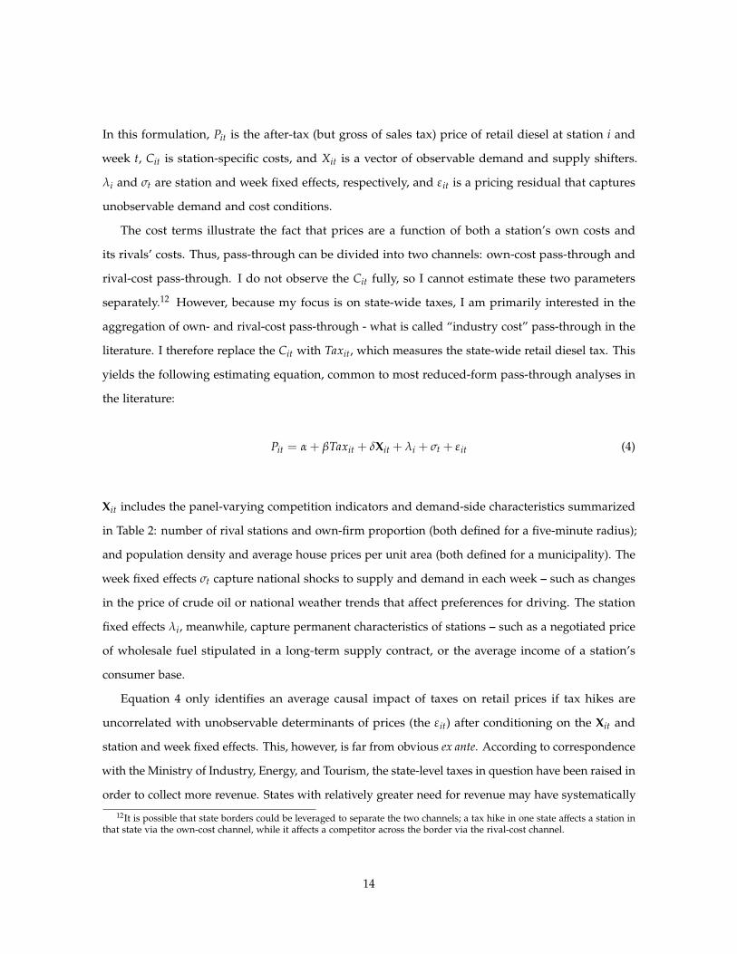
In this formulation, Pit is the after-tax (but gross of sales tax) price of retail diesel at station i and

week t, Cit is station-specific costs, and Xit is a vector of observable demand and supply shifters.

λi and σt are station and week fixed effects, respectively, and εit is a pricing residual that captures

unobservable demand and cost conditions.

The cost terms illustrate the fact that prices are a function of both a station’s own costs and

its rivals’ costs. Thus, pass-through can be divided into two channels: own-cost pass-through and

rival-cost pass-through. I do not observe the Cit fully, so I cannot estimate these two parameters

separately.12 However, because my focus is on state-wide taxes, I am primarily interested in the

aggregation of own- and rival-cost pass-through - what is called “industry cost” pass-through in the

literature. I therefore replace the Cit with Taxit, which measures the state-wide retail diesel tax. This

yields the following estimating equation, common to most reduced-form pass-through analyses in

the literature:

Pit = α + βTaxit + δXit + λi + σt + εit (4)

Xit includes the panel-varying competition indicators and demand-side characteristics summarized

in Table 2: number of rival stations and own-firm proportion (both defined for a five-minute radius);

and population density and average house prices per unit area (both defined for a municipality). The

week fixed effects σt capture national shocks to supply and demand in each week – such as changes

in the price of crude oil or national weather trends that affect preferences for driving. The station

fixed effects λi, meanwhile, capture permanent characteristics of stations – such as a negotiated price

of wholesale fuel stipulated in a long-term supply contract, or the average income of a station’s

consumer base.

Equation 4 only identifies an average causal impact of taxes on retail prices if tax hikes are

uncorrelated with unobservable determinants of prices (the εit) after conditioning on the Xit and

station and week fixed effects. This, however, is far from obvious ex ante. According to correspondence

with the Ministry of Industry, Energy, and Tourism, the state-level taxes in question have been raised in

order to collect more revenue. States with relatively greater need for revenue may have systematically

12It is possible that state borders could be leveraged to separate the two channels; a tax hike in one state affects a station inthat state via the own-cost channel, while it affects a competitor across the border via the rival-cost channel.

14

different price trends from other states; this is one example of how pass-through estimation via

the above equation could be invalidated. Moreover, even if treated states exhibit trends that are

parallel to untreated ones, my analysis could be compromised if I do not account for potential

anticipatory market responses to tax hikes. Coglianese et al. (2015) show that U.S. consumers adjust

their consumption of gasoline upwards one month in advance of tax hikes and downwards in the

first month of the new tax level. While they fail to find corresponding adjustments in retail prices,

the fact remains that tax hikes are anticipated.

4.1 Event study

To explore the viability of Equation 4 in identification of pass-through, I first estimate an event study

model of price trends in the vicinity of tax changes. Event study provides a sense of pre-existing

pricing patterns in locations experiencing a tax change, as well as the timing of a market’s response to

such a tax change. Its purpose is thus diagnostic - I use it only to assess the potential for endogeneity

and anticipation, not to quantify pass-through.

4.1.1 Model

A natural starting point for event study of diesel tax hikes in Spain is the following model:

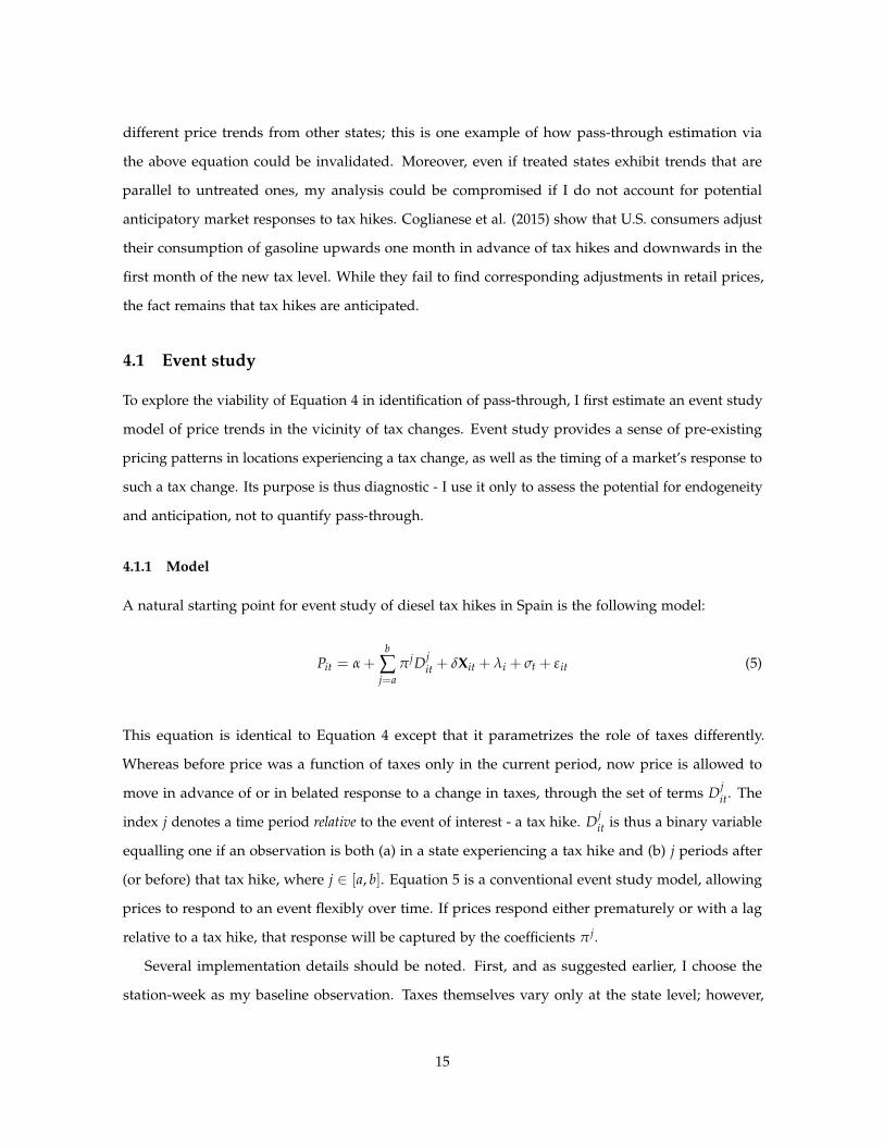
Pit = α +b

∑j=a

π jDjit + δXit + λi + σt + εit (5)

This equation is identical to Equation 4 except that it parametrizes the role of taxes differently.

Whereas before price was a function of taxes only in the current period, now price is allowed to

move in advance of or in belated response to a change in taxes, through the set of terms Djit. The

index j denotes a time period relative to the event of interest - a tax hike. Djit is thus a binary variable

equalling one if an observation is both (a) in a state experiencing a tax hike and (b) j periods after

(or before) that tax hike, where j ∈ [a, b]. Equation 5 is a conventional event study model, allowing

prices to respond to an event flexibly over time. If prices respond either prematurely or with a lag

relative to a tax hike, that response will be captured by the coefficients π j.

Several implementation details should be noted. First, and as suggested earlier, I choose the

station-week as my baseline observation. Taxes themselves vary only at the state level; however,

15

competition is a much more local phenomenon in retail automotive fuel markets. Meanwhile, the

week level balances high resolution of analysis with computational tractability. Second, I choose [a, b]

to be equal to [−12, 12], which is an observation window of 6 months, and omit the term π0D0it so that

the price impact in the week of the tax hike is normalized to zero. Third, I use all weeks from January

2007 through June 2013, regardless of their temporal proximity to tax hikes; this helps pin down my

time fixed effects but necessitates the creation and inclusion of two dummy variables: one for an

observation being from a period j < −12, and one for an observation being from a period j > 12.

Fourth, I use all states, regardless of whether they are “treated” (with a tax hike) or “untreated”.13

Fifth, and finally, I cluster standard errors at the state level.

4.1.2 Findings

Figure 6 graphically depicts the results of the event study estimation of Equation 5. Each plotted

y-value is the average value of(

π jDjit

EventSizejit

), which is the price predicted in a location i that has been

(or is going to be) subject to a tax hike in period t + j. The y-value in week 0 is normalized to zero, so

every other plotted point represents the predicted price relative to that initial week of the tax hike.

If there were observable trends or movements in the predicted price before tax changes take effect,

these would raise concerns about the exogeneity of the tax changes. That is not the case here. Figure

6 exhibits extremely flat trends in prices both before and after the tax event. The only time period

with any slope at all is a three-week period surrounding the tax event. Most of the price jump occurs

in week 0 itself - right when the tax changes; however, there are rises in the week prior and the week

after as well. I interpret these movements as evidence that the market anticipates tax hikes by one

week and takes one additional week after the hike itself to fully re-equilibrate.

The evidence strongly suggests that the retail price response to a tax hike is a mean shift. This

observation, in turn, motivates a fixed effects regression model to identify the actual pass-through

rate. Of course, Figure 6 does strongly hint at what this rate is: a comparison of the plotted price

levels before the event with price levels after the event suggests a gap of at least 0.9 – i.e., average

retail price rises 0.9 c/L for every 1 c/L of a tax hike – which translates directly to a pass-through

rate of at least 90%. This estimate, as well as the pre- and post-trends estimated, is robust to a variety

of specifications. The results hold for alternative event study models;14 they hold at several different

13Estimation is also possible using only treated states, but this requires an additional parametric assumption (see McCrary2007).

14Equation 5 is, to my knowledge, consistent with all other published event studies in the economics literature, in thatit parameterizes the event of interest as a dummy variable. This is equivalent to modeling only the extensive margin

16

levels of observation;15 and they hold with sample restrictions that exclude observations from outside

of the six-month window of a local tax hike.

4.2 Difference-in-Difference Regression

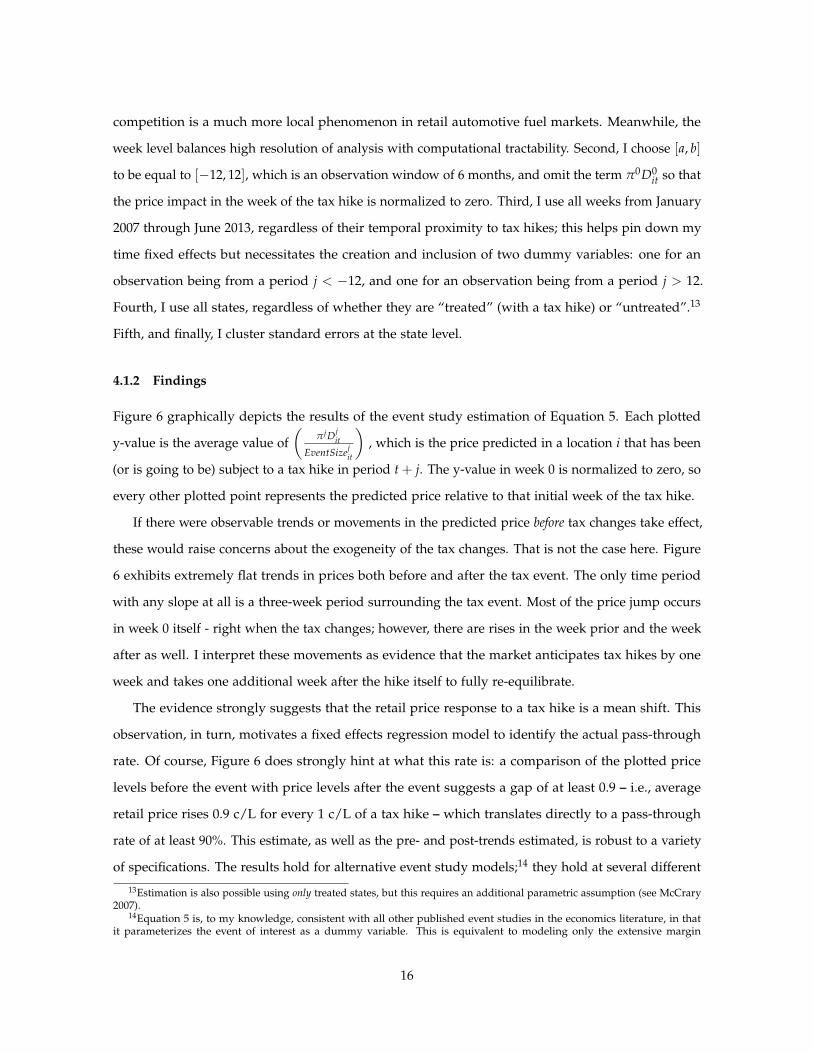
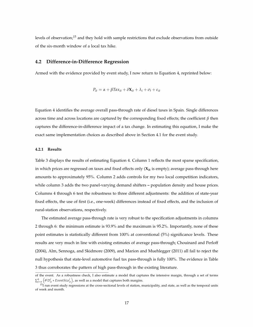
Armed with the evidence provided by event study, I now return to Equation 4, reprinted below:

Pit = α + βTaxit + δXit + λi + σt + εit

Equation 4 identifies the average overall pass-through rate of diesel taxes in Spain. Single differences

across time and across locations are captured by the corresponding fixed effects; the coefficient β then

captures the difference-in-difference impact of a tax change. In estimating this equation, I make the

exact same implementation choices as described above in Section 4.1 for the event study.

4.2.1 Results

Table 3 displays the results of estimating Equation 4. Column 1 reflects the most sparse specification,

in which prices are regressed on taxes and fixed effects only (Xit is empty); average pass-through here

amounts to approximately 95%. Column 2 adds controls for my two local competition indicators,

while column 3 adds the two panel-varying demand shifters – population density and house prices.

Columns 4 through 6 test the robustness to three different adjustments: the addition of state-year

fixed effects, the use of first (i.e., one-week) differences instead of fixed effects, and the inclusion of

rural-station observations, respectively.

The estimated average pass-through rate is very robust to the specification adjustments in columns

2 through 6: the minimum estimate is 93.9% and the maximum is 95.2%. Importantly, none of these

point estimates is statistically different from 100% at conventional (5%) significance levels. These

results are very much in line with existing estimates of average pass-through; Chouinard and Perloff

(2004), Alm, Sennoga, and Skidmore (2009), and Marion and Muehlegger (2011) all fail to reject the

null hypothesis that state-level automotive fuel tax pass-through is fully 100%. The evidence in Table

3 thus corroborates the pattern of high pass-through in the existing literature.

of the event. As a robustness check, I also estimate a model that captures the intensive margin, through a set of terms

∑bj=a

(θ jDj

it ∗ EventSizejit

), as well as a model that captures both margins.

15I run event study regressions at the cross-sectional levels of station, municipality, and state, as well as the temporal unitsof week and month.

17

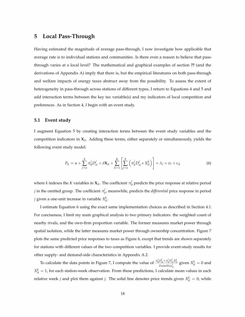
5 Local Pass-Through

Having estimated the magnitude of average pass-through, I now investigate how applicable that

average rate is to individual stations and communities. Is there even a reason to believe that pass-

through varies at a local level? The mathematical and graphical examples of section ?? (and the

derivations of Appendix A) imply that there is, but the empirical literatures on both pass-through

and welfare impacts of energy taxes abstract away from the possibility. To assess the extent of

heterogeneity in pass-through across stations of different types, I return to Equations 4 and 5 and

add interaction terms between the key tax variable(s) and my indicators of local competition and

preferences. As in Section 4, I begin with an event study.

5.1 Event study

I augment Equation 5 by creating interaction terms between the event study variables and the

competition indicators in Xit. Adding these terms, either separately or simultaneously, yields the

following event study model:

Pit = α +b

∑j=a

πj0Dj

it + δXit +K

∑k=1

[b

∑j=a

(π

jkDj

it ∗ Xkit

)]+ λi + σt + εit (6)

where k indexes the K variables in Xit. The coefficient πj0 predicts the price response at relative period

j in the omitted group. The coefficient πjk, meanwhile, predicts the differential price response in period

j given a one-unit increase in variable Xkit.

I estimate Equation 6 using the exact same implementation choices as described in Section 4.1.

For conciseness, I limit my main graphical analysis to two primary indicators: the weighted count of

nearby rivals, and the own-firm proportion variable. The former measures market power through

spatial isolation, while the latter measures market power through ownership concentration. Figure 7

plots the same predicted price responses to taxes as Figure 6, except that trends are shown separately

for stations with different values of the two competition variables. I provide event-study results for

other supply- and demand-side characteristics in Appendix A.2.

To calculate the data points in Figure 7, I compute the value of πj0Dj

it+πjk Dj

itXkit

EventSizejit

given Xkit = 0 and

Xkit = 1, for each station-week observation. From these predictions, I calculate mean values in each

relative week j and plot them against j. The solid line denotes price trends given Xkit = 0, while

18

the dashed line pertains to Xkit = 1. A comparison of these two lines tests whether a gas station’s

temporal response to taxes varies with its local competitive environment.

Figure 7 shows that pre- and post-trends are flat. Stations of different types do not seem to

respond differentially over time to tax hikes. Rather, both panels show two trends moving in striking

parallel. Figure 7 does not, on its own, prove the exogeneity of brand and location, as these may

still be cross-sectionally correlated with unobserved determinants of pass-through. However, it is

clear that the mean shift categorization of average pass-through in Figure 7 holds across different

competitive environments. I therefore deem a fixed-effects specification suitable for quantifying the

difference in pass-through rates predicted by competition indicators.

The plotted trends do, however, provide early indication of a relationship between pass-through

and local competition. The gap between trends at a station with no rivals and a station with weighted

rival count equal to one narrows. Meanwhile, the gap between the zero-concentration trend and

the effective-monopoly trend widens immediately after tax hikes. Both trends suggest a positive

relationship between market power and pass-through; I use fixed effects to quantify that relationship.

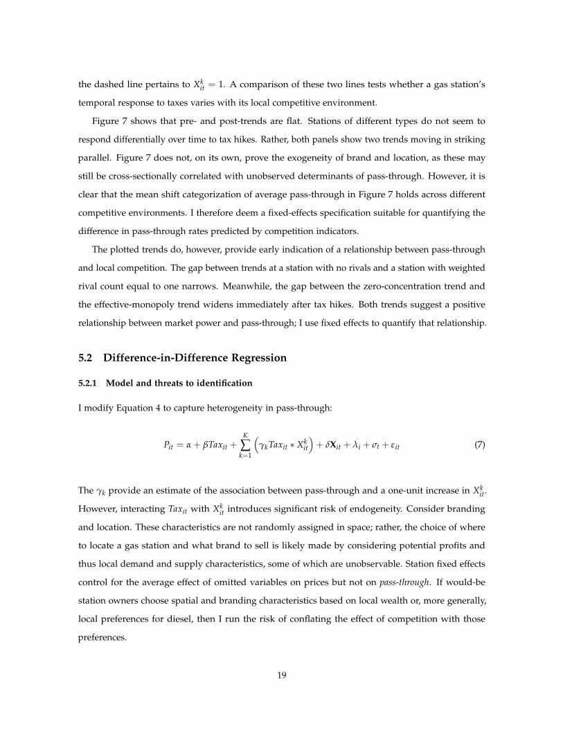
5.2 Difference-in-Difference Regression

5.2.1 Model and threats to identification

I modify Equation 4 to capture heterogeneity in pass-through:

Pit = α + βTaxit +K

∑k=1

(γkTaxit ∗ Xk

it

)+ δXit + λi + σt + εit (7)

The γk provide an estimate of the association between pass-through and a one-unit increase in Xkit.

However, interacting Taxit with Xkit introduces significant risk of endogeneity. Consider branding

and location. These characteristics are not randomly assigned in space; rather, the choice of where

to locate a gas station and what brand to sell is likely made by considering potential profits and

thus local demand and supply characteristics, some of which are unobservable. Station fixed effects

control for the average effect of omitted variables on prices but not on pass-through. If would-be

station owners choose spatial and branding characteristics based on local wealth or, more generally,

local preferences for diesel, then I run the risk of conflating the effect of competition with those

preferences.

19

In the case of station location, correlation with unobservable determinants of demand would

most likely bias estimates of γk in Equation 7 upwards. This is because station owners presumably

prefer, all else equal, to locate in areas with more inelastic demand, which itself drives pass-through

upwards. The prediction for endogenous brand (and contract) choice is less clear, as it depends on

the strategy of each specific brand. If, for example, a certain brand likes to concentrate in areas with

more inelastic demand, then parameter estimates corresponding to that brand’s concentration may be

biased upwards. However, if all brands would like to locate in these areas, then it is not clear which

precise branding pattern emerges, and the potential bias is difficult to sign.

The demand attributes faced by specific stations are inherently difficult to measure, especially

because consumers sort into stations based on commuting patterns and willingness to price-shop.

However, controlling for group-average observables has the potential to absorb much of the selection

of my competition “treatments” on unobservables (Altonji and Mansfield 2015). I therefore compare

results of estimation of Equation 7 using just competition interactions versus additionally including

interactions with my observable proxies of demand: population density, house prices, and education

levels. House prices act as a city-level proxy for wealth; robustness to their inclusion would suggest

my competition results are not being driven by the average wealth of a station’s municipality. Similarly,

insofar as population density is a proxy for infrastructure investments like public transit, robustness to

the inclusion of an interaction between it and the tax would suggest that my results are not driven by

certain stations locating in areas with fewer transportation alternatives. Finally, interactions between

the tax and indicators of educational attainment allow a robustness test using a very different level

of variation – the educational indicators that I use are cross-sectional (from 2011), but they are also

disaggregated to the 1-km2 geographic level. Thus, if stations choose brands and/or locations based

on the preferences of the population living in the immediate vicinity, then I can control for the part of

those preferences that is correlated with education. More generally, my underlying logic is that, even

if house prices, population density, and education do not fully absorb selection on unobservables,

they remain useful as a guide to the degree to which remaining selection might affect my estimates

(Altonji, Elder, and Taber 2005). If one assumes that the effect of unobservable aspects of demand is

bounded above by the effect of observable aspects, then the change in point estimates brought about

by inclusion of observables is equal to that upper bound.

20

5.2.2 Results

Table 4 provides point estimates on each interaction of interest separately. In column 1, branding is

the characteristic in focus; in column 2, it is the number and proximity of rival stations; in column

3, it is the proportion of nearby stations under the same ownership as the reference station; and in

column 4, it is the average house price of a municipality.

Each indicator (except for the wholesaler-brand dummy) is a statistically significant predictor

of pass-through when examined separately. All are significant at the 5% level, while three of the

four are significant at the 1% level. The refiner-brand point estimate has the following interpretation:

switching from being unbranded to bearing the brand of a refiner is associated, on average, with a

rise in pass-through of 13.8 percentage points. Meanwhile, pass-through drops an average of 11.7

percentage points per each one-unit increase in weighted rival count. Since the latter variable runs

from 0 to ∼ 2 in the data, the implication is that concentrated spatial competition can potentially

reduce pass-through by as much as ∼ 23.4 percentage points. Concentrated ownership also is

associated with higher pass-through: a local monopoly (own-firm proportion=1) is associated with a

pass-through rate 17 percentage points higher than a station with negligible concentration (own-firm

proportion→0). Finally, a one-unit rise in average house prices predicts a 22 percentage-point rise in

pass-through.

The column 1 result suggests that something about refiner brands – whether it is market power

generated by brand loyalty, the degree of vertical integration, or some other factor – drives pass-

through upwards. Columns 2 and 3 indicate possible effects of market power through spatial isolation

(column 2) and ownership concentration (column 3). Column 4 shows that areas with higher property

values are, for one reason or another, places with larger price impacts of taxation. These coefficients

are strong motivation for continued study of local pass-through patterns, but they are also estimated

in isolation. For simultaneous estimation, I move on to Table 5.

Column 1 of Table 5 shows the results of simultaneous estimation of three competition variables in

5. Each coefficient is reduced in magnitude to some degree, but all remain statistically significant. In

particular, the refiner-brand indicator and the rival count variable retain their statistical significance at

the 1% level and imply predictive effects of over 10 percentage points on pass-through for a one-unit

change in their values. The coefficient on own-firm proportion, meanwhile, drops from 0.17 to 0.11

but is still significant at the 5% level.

Columns 2 through 4 successively add other observable indicators of both the supply side and

21

the demand side. Column 2 includes interaction terms between the tax and four station amenities:

carwash services, tire and fluid services, convenience store, and cafeteria. The inclusion of these

variables shows whether the results for my primary competition indicators are driven by differences

in the services provided by each station. The point estimates in column 2 suggest that this is not the

case; conditional on the effect of station amenities, pass-through is still strongly associated with a

gas station’s brand, its spatial isolation, and the extent of shared ownership in its vicinity. The same

can be said after including indicators of local refiner-brand and wholesaler-brand proportions and a

Herfindahl Hirschman Index, as is done in column 3. The addition of these variables is motivated by

the significance of the own-brand market power measures; if, e.g., one’s own connection to a refiner

brand is important, then perhaps the connection of other nearby stations is also important. In that

case, the coefficient on own-firm proportion could be driven not by shared ownership generally but

by the intensity of refiner-brand activity specifically. Column 3 suggests that even conditional on

local refiner-brand proportion, own-firm proportion remains statistically significant.

Column 4, however, is the truest test of the robustness of my measured competition effects. In

this column I include interactions between the tax and my three demand-side characteristics: average

house prices, population density, and educational attainment. These are, of course, mere proxies for

the wealth, consumption base, and public transit infrastructure that more directly affect demand; I

am unable to completely control for the effect of the demand side on pass-through. Robustness of my

competition results to the inclusion of these demand shifters is therefore not a sufficient condition for

a causal interpretation. However, it is a necessary condition. Furthermore, the degree to which my

point estimates and their significance drop in response to the new demand-side variables provides a

guide to the remaining bias due to omitted variables.

Observable characteristics of local consumers do not, according to column 4, affect the size

or significance of competition effects in a meaningful way. The coefficients on refiner brand and

rival count drop approximately two percentage points but still imply economically significant 9-9.5

percentage-point impacts in pass-through per unit change. The coefficient on own-firm proportion

actually rises in significance, from the 10% level to the 5% level. The fact that refiner brand, rival

count, and own-firm proportion move only minimally while retaining high economic and statistical

significance suggests that the effect of unobservable market conditions would have to be a good deal

larger than the effect of observable ones in order to negate such significance. The evidence supporting

a causal impact of local competition is therefore strong.

22

In the case of refiner branding, it is difficult to explain the precise mechanism of the pass-through

impact. Two possible explanations are that customers have brand loyalty that creates market power

for larger brands (60% of Spanish stations are refiner-branded), and that vertical integration by a retail

gas station and an upstream refiner changes either the cost structure or the retail pricing strategy

employed. In the case of own-firm proportion and rival-station count, the identified impacts are

most easily explained by traditional market power stories. A firm owning multiple stations in the

same area may have a stronger incentive to raise prices in response to a cost shock, because the sales

lost from these price hikes at any one of its stations will partially be recouped by its other stations.

Meanwhile, a lack of spatial competition may have a similar incentive effect, because consumers have

fewer options for switching away from their usual station when its prices rise. Through both both

of these channels – branding patterns and spatial isolation – market power thus appears to raise

pass-through.

Two further specifications, whose results are shown in columns 5 and 6 of Table 5, provide

additional robustness checks. Column 5 displays results of estimation with state-year fixed effects.

All three key competition indicators remain significant, though their relative importance changes

slightly – the own-firm proportion coefficient becomes significant at the 1% level, while the rival-count

coefficient drops in magnitude to a 5.4 percentage-point effect and is significant at only the 5% level.

Column 6, in contrast, uses the whole of Spain in estimation. To run this regression, I must omit two

of my demand shifters (house prices and education levels), but the results are nonetheless informative.

The three key competition indicators remain statistically significant, while, as suggested in Section

3, the point estimates on variables corresponding to gas stations’ surroundings are much noisier.

Interestingly, all of the competition indicators examined in this table are significant when the full

national panel is used.

Lastly, but not least importantly, the interaction between the diesel tax and municipal-average

house prices is very significant, both economically and statistically, according to my preferred

specification in column 4. A one-unit change in the house-price variable corresponds to a 1,000

Euro/m2rise, in a measure whose standard deviation is 640 Euro/m2 (as shown in Table 2). This one-

unit change is associated with a 19.5 percentage-point increase in pass-through which is statistically

significant at the 1% level. I do not make any claim on causality here; many things are correlated

with house prices. However, insofar as house prices are a proxy for lifetime wealth, my result has

significant implications for the joint distribution of wealth and the price impacts of taxation. I return

23

to this idea in detail in Section 6.

5.3 The empirical distribution of pass-through

Regardless of whether the effects identified in Table 5 have a causal interpretation, they provide

strong evidence that pass-through is heterogeneous. Ultimately, the point of this research is to show

that pass-through varies from location to location; distributional analyses that assume away this

heterogeneity run the risk of yielding inaccurate results. How significant could this innacuracy

be? To begin answering this question, I use my estimated coefficients to calculate station-specific

pass-through rates and graph them to explore their overall distribution.

I calculate station-specific price impacts as the linear combination of the predictive effects of all

tax terms – βTaxit + ∑Kk=1

(γkTaxit ∗ Xk

it

)in Equation 7 above. I divide this value by Taxit to yield an

estimate of pass-through dpitdtst

for each station i in week t. In Figure 8, I plot these rates on the last

day of observation for each station, using a kernel density estimator. Not surprisingly, the central

tendency is 91% pass-through. However, the full range of observed pass-through rates ranges from

50% to 150%. 95% of these rates fall between 72% and 115%.

It is natural to ask how much of the pass-through distribution’s spread is due simply to noise. To

answer this question, I calculate the empirical variance of the pass-through rates used in Figure 8 and

subtract off an estimate of noise. To estimate noise, I compute the standard error of each station’s

pass-through estimate, square it, and take the average across all stations. As the top-right corner of

Figure 8 indicates, removing noise drops the standard deviation of the station pass-through rate from

a raw value of 13.2 to an adjusted value of 12.3. That change corresponds to a contraction in the 95%

confidence range of about 4 percentage points16.

Pass-through patterns provide indirect insight into the nature of demand for automotive fuel. 24%

of retail gas stations pass-through more than 100% of taxes to end consumers; this fact is inconsistent

with both perfect competition and linear demand, both of which are common assumptions in the

energy tax incidence literature. The most plausible explanation for rates above 100% is a setting of

imperfect competition and sufficiently convex demand (like the isoelastic demand curve plotted in

Figure 1). Other possible explanations – such as a lack of salience of taxes that drives consumers

to under-respond to tax movement (Chetty, Looney, and Kroft 2009) – are less likely to be relevant,

given the tax-inclusive nature of posted prices.

16While there is additional noise coming from the explanatory variables themselves, it is more than counteracted byattenuation of the estimates due to measurement error.

24

In sum, both local preferences and competition levels appear to play a significant role in deter-

mining rates of energy tax pass-through in the Spanish diesel market. The analysis suggests that,

from station to station and from market to market, there can exist extremely large differences in the

size of the consumer tax burden. In the next section, I explore what this means for policy design and

assessment.

6 Pass-Through and the Wealth Distribution

How does pass-through heterogeneity affect who ultimately bears the burden of automotive fuel

taxes? The average pass-through rate is most commonly used to provide insight into the consumer-

producer breakdown of the tax burden, but station-specific rates allow me to compare burdens across

different consumer groups. I focus on wealth, since regressive incidence across the wealth distribution

is one of the most oft-cited properties of energy taxes.

The consensus finding in the energy tax incidence literature (described above in Section ??) is that

such taxes are regressive. This is generally due to the fact that poorer houesholds are observed to

spend a greater portion of their wealth on energy, at least in the U.S. However, several factors that

mitigate this regressivity have been identified. First of all, regressivity estimates are sensitive to the

specification of wealth; Poterba (1991) shows that annual expenditure is a better proxy for lifetime

wealth than annual income, and that using the former leads to smaller magnitudes of regressivity in

the U.S. gasoline tax. Second of all, the poorest households often do not own energy capital such as

automobiles; including these households in analysis can vastly reduce regressivity (Fullerton and

West 2003), especially in the developing country context (Blackman, Osakwe, and Alpizar 2009).

Third of all, the demand response to taxes is unlikely to be static across the wealth distribution; West

(2004) and West and Williams (2004) estimate that the gasoline demand elasticity drops (in absolute

magnitude) as income rises in the U.S., which makes consumer surplus impacts less regressive than

when demand response is assumed to be homogeneous.

One of the primary contributions of this paper is to add a fourth-mitigating factor: pass-through

heterogeneity. Just like the demand elasticity – indeed, because of the demand elasticity – pass-through

need not be static across the wealth spectrum. In fact, pass-through heterogeneity is likely to have a

much greater effect on tax incidence than corresponding heterogeneity in demand elasticity, because

the welfare lost due to higher prices on maintained consumption probably dwarfs the welfare lost

25

from consumption foregone. In my own context, I find economically significant variation in pass-

through rates across the house-price distribution. Pass-through rises in municipal wealth, and this, in

turn, should make the retail diesel tax relatively less regressive (or more progressive).

Return to Figure 1 to see the direct consumer surplus impacts of a tax hike shaded in gray. I

do not estimate the demand curve itself, so I am unable to calculate the deadweight loss triangle

component. However, pass-through provides traction for estimation of the rectangular component,

which is the welfare lost from consumption maintained in the face of the tax hike. For small changes,

this rectangle is mathematically the first-order approximation of consumer surplus impacts. Given

low elasticities of demand for retail energy, it is also likely the larger of the two welfare components17.

Pass-through measures the height of the rectangle, so combining it with a measure of the width (i.e.,

consumption) allows for calculation of the rectangle’s area – dpdt Q1.

In distributional welfare analysis, the goal is compare the size of consumer surplus impacts across,

e.g., the wealth spectrum. In the absence of a demand curve, the most common method of assessing

regressivity is a comparison ofdpdt Q1W across quantiles of wealth W. Dividing by W converts consumer

surplus changes to proportions of total wealth. Examples of this in the context of automotive fuel

taxation are Poterba (1991) and Fullerton and West (2003). The Treasury Department’s Office of Tax

Analysis does the same for its own estimates of tax burdens (Fullerton and Metcalf 2002).

Ifdpdt Q1W rises with wealth decile, then tax t is progressive; if it falls, then t is regressive. In

practice, the latter is almost always true, at least for some portion of the wealth distribution. However,

implementation of the exercise has, to date, relied on an assumption of full, uniform pass-through –

i.e., dpdt is identically 1 and does not vary with wealth. The expression then collapses to Q1

W , which

accurately captures tax revenues per unit consumption but is only proportion to tax burden if pass-

through is uniform18. This is precisely the opposite of what I find empirically in Spain’s retail diesel

market.

To show the effect of systematic variation in pass-through with wealth, I carry out the incidence

calculation both with and without the assumption of uniform pass-through, using data from the 2013

Spanish Household Budget Survey (Encuesta de Presupuestos Familiars (EPF)). I divide households’

fuel consumption Q (in liters) by their overall expenditure E – a smoother proxy for wealth than

17Equivalently, it is likely that the first ’cost’ on a car owner’s mind when a tax is raised is the extra cost paid for all thegasoline that he/she will continue to purchase, rather than the utility lost from reducing purchases.

18Moreover, data limitations mean that implementation usually relies on expenditure of energy rather than consumption.fuel expenditure is only proportional to fuel consumption if prices are the same for all households, so the calculation relies onan unrealistic assumption of uniform pricing.

26

income (Poterba 1991) – and collapse these values into averages within each decile of overall

expenditure. As is, these average values of QE can be interpreted as estimates of the government

revenues generated by households per unit tax hike, as a proportion of their overall wealth.

I then replicate the calculation while relaxing the assumption of uniform pass-through. This, of

course, requires estimates of pass-through corresponding to wealth, of the form

τ = α + βQE + ε (8)

where τ is pass-through and QE is a quantile (decile) of household expenditure. I do not jointly

observe (τ, QE). Instead, I observe (τ, QHP), where QHP is the average house-price decile. The two

proxies for wealth are related as follows:

QE = a + bQHP + e (9)

I estimate pass-through as a function of house prices rather than expenditure, which is equivalent to

substitution of Equation 9 into Equation 8. This yields

τ = α + aβ + βbQHP + ε + βe (10)

The coefficient on QHP underestimate the magnitude of the the rise in pass-through with wealth to

the extent that b < 1, as would occur due to measurement error.

However, QHP is unlikely to be a valid instrument for QE, because house prices are additionally

correlated with pass-through for unobserved reasons that have little do with income. For instance,

some poorer people live in richer neighborhoods, and vice versa. The extent to which poorer

individuals are forced to buy automotive fuel in richer areas is likely mitigated to some degree by

sorting: some consumers like to price shop, and applications like Gas Buddy in the U.S. and Spain’s

own Geoportal target precisely those consumers. Moreover, demand estimation in the industrial

organization literature nearly always finds a lower disutility of price among richer individuals (again,

see Houde 2012 for an example). Still, βb may be overestimated on net due to incomplete sorting.

I nonetheless proceed with the exercise, to illustrate how large variation in local pass-through

27

rates can translate to welfare impacts. The regression analog of Equation 10 is below:

Pit = α + β1Taxit +10

∑D=2

(βDTaxit ∗ 1[HPDecile = D]it) + δXit + λi + σt + εit (11)

The coefficients β1 and βD provide estimated pass-through rates corresponding to each decile of the

house price distribution. These rates are then used to computedpdt QE at different expenditure deciles.

Figure 9 plots the proportional tax burdens with and without the pass-through adjustment.

Interestingly, when pass-through is assumed full and uniform (solid line), households appear to have

roughly equal fuel tax burdens as a proportion of their full budget (i.e., equal fuel-tax rates). Incidence

is neither regressive nor progressive in this formulation of the exercise. This pattern runs counter

to the belief that poorer households spend more of their budget on fuel than richer ones, which

would yield a downward-sloping graph in Figure 9. Understanding the flat trend with respect to

Spanish automotive fuel consumption is thus a subject for further research; however, the main point of

Figure 9 is the effect of heterogeneous pass-through relative to this flat baseline. When pass-through

heterogeneity is explicitly accounted for in analysis (dashed line), higher-expenditure households

appear to have much higher effective fuel-tax rates. Incidence now looks strongly progressive.

While the magnitude of the pass-through effect on progressivity is large, it should not be surprising.

Pass-through is inherently related to demand elasticity, so the pass-through/wealth relationship is

inseparable from the demand elasticity/wealth relationship. Some have argued that richer people are

more sensitive to fuel prices than poorer ones (Keyser 2000; Hughes, Knittel, Sperling 2008), because,

for example, the rich have more “discretionary” uses of automotive fuel. A large body of research

in the structural industrial organization literature, however, suggests that disutility of prices falls

in income (e.g., Houde 2012), which implies less price sensitivity among the rich. Furthermore, the

effect of variable demand elasticities is the focal point of research by West (2004) and by West and

Williams (2004); they estimate that demand for gasoline is more inelastic in richer areas. My findings

are consistent with this result; a question for future research is, does pass-through rise in wealth for

taxes on other goods, in other markets and countries?

28

7 Conclusion

In this paper, I have leveraged highly detailed data from the Spanish retail automotive fuel market

to investigate the price impacts of energy taxes. My primary tool for this investigation has been

pass-through – the degree to which taxes physically imposed on retail gas stations are passed through

to final consumers. While there are dozens of published studies of energy tax pass-through, my

research uniquely focuses on competition and local preferences as determinants of the pass-through

parameter. I estimate station-specific pass-through rates, which I find to vary widely around a central

tendency of 90-95%, from at least 70 to 115%. On the competition side, pass-through rises significantly

when a station bears the brand of a vertically-integrated refiner, when it is spatially isolated, and

when it shares an owner with other stations in its vicinity. On the demand side, pass-through rises

steeply with municipal-average house prices, which are a good proxy for lifetime wealth.

These results have major implications for the distributional impacts of the diesel tax in question

and energy taxes more generally. Because pass-through measures the extra cost that a consumer

must pay for his or her automotive fuel, per unit tax, it has great power to describe the welfare

impacts of taxation. Heterogeneous pass-through, unaccounted for, will always lead to mistaken

estimates (and forecasts) of these welfare impacts at a local geographic level. Since pass-through

is positively correlated with wealth in Spain, ignoring pass-through heterogeneity in this context

will produce estimates that are not just mistaken, but also biased. I illustrate this by estimating

marginal tax burdens by the average household in each decile of the wealth distribution, both with

and without an assumption of uniform pass-through. What looks like a policy with roughly flat

incidence across the wealth distribution becomes a strongly progressive policy when my empirically

estimated pass-through rates are factored into the calculation.

An accurate picture of the distributional impacts of energy taxes is important because of

widespread reliance on these taxes across the world and the potential for even more. For in-

stance, a recent drop in retail gasoline prices in the U.S. has precipitated calls for both a higher federal

gas tax (Washington Post 2015a) and the establishment of a federal carbon tax (Washington Post

2015b). The realization of these policy recommendations hinges on their political feasibility, which is

in part a function of distributional equity. Moreover, regardless of whether such policy changes are

absolutely progressive or regressive, it is vital to know who bears what burden so that redistribution

can accurately target those who are most adversely affected.

My analysis of pass-through has implications not just for distributional equity, but also for

29

economic efficiency. The evidence strongly suggests that competition in such markets is highly

imperfect. Thus, the traditional notion of optimal Pigouvian tax levels being equal to the social

marginal cost of the relevant externalities no longer holds. The fact of market power in markets for

retail automotive fuel implies that prices are already above private marginal costs, so the optimal

Pigouvian tax is now lower than the social marginal cost of consumption.

Pass-through thus has great potential as a tool of economic analysis. While a full estimation

of demand and supply curves would obviate the need to focus on pass-through, the data and

computational challenges of such estimation make reduced-form pass-through analysis a worthwhile

endeavor. Its accurate estimation, especially at a local level, facilitates a greater understanding of

optimality, distributional equity, and the way in which firms compete.

30

References

[1] Aguirre, Iñaki, Simon Cowan, and John Vickers. 2010. “Monopoly Price Discrimination and

Demand Curvature.” American Economic Review 100(4):1601-1615.

[2] Alm, James, Edward Sennoga, and Mark Skidmore. 2009. “Perfect Competition, Urbanization,

and Tax Incidence in the Retail Gasoline Market”. Economic Inquiry 47(1): 118-134.

[3] Auer, Raphael A. and Raphael S. Schoenle. 2013. “Market Structure and Exchange Rate Pass-

Through.” Mimeo.

[4] Altonji, Joseph G., Todd E. Elder, and Christopher R. Taber. 2005. “Selection on Observed

and Unobserved Variables: Assessing the Effectiveness of Catholic Schools.” Journal of Political

Economy 113(1): 151-184.

[5] Anderson, Simon P., André de Palma, and Brent Kreider. 2001. “Tax Incidence in Differentiated

Product Oligopoly”. Journal of Public Economics 81: 173-192.

[6] Bello, Alejandro and Ignacio Contín-Pilart. 2012. “Taxes, cost and demand shifters as determi-

nants in the regional gasoline price formation process: Evidence from Spain.” Energy Policy 48:

439-448.

[7] Bento, Antonio M., Lawrence H. Goulder, Emeric Henry, Mark R. Jacobsen, and Roger H. von

Haefen. 2009. “Distributional and Efficiency Impacts of Gasoline Taxes: An Econometrically

Based Multi-Market Study”. American Economic Review: Papers and Proceedings 95(2): 282-287.

[8] Bento, Antonio M., Lawrence H. Goulder, Mark R. Jacobsen, and Roger H. von Haefen. 2009.

“Distributional and Efficiency Impacts of Increased US Gasoline Taxes”. American Economic Review

99(3): 667-699.

[9] Besley, Timothy J. and Harvey S. Rosen. 1999. “Sales Taxes and Prices: An Empirical Analysis”.

National Tax Journal 52(2): 157-178.

[10] Blackman, Allen, Rebecca Osakwe, and Francisco Alpizar. 2009. “Fuel Tax Incidence in Develop-

ing Countries: The Case of Costa Rica”. Resources For the Future Discussion Paper 09-37.

[11] Bulow, Jeremy I. and Paul Pfleiderer. 1983. “A Note on the Effect of Cost Changes on Prices”.

Journal of Political Economy 91(1): 182-185.

31

[12] Chetty, Raj, Adam Looney, and Kory Kroft. 2009. “Salience and Taxation: Theory and Evidence”.

American Economic Review 99(4): 1145-1177.

[13] Chouinard, Hayley and Jeffery M. Perloff. 2004. “Incidence of Federal and State Gasoline Taxes”.

Economics Letters 83: 55-60.

[14] Coglianese, John, Lucas W. Davis, Lutz Kilian, and James H. Stock. 2015. “Anticipation, Tax

Avoidance, and the Price Elasticity of Gasoline Demand”. Harvard Environmental Economics

Program Discussion Paper 15-61.

[15] Contín-Pilart, Ignacio, Aad F. Correljé, and M. Blanca Palacios. 2009. “Competition, regulation,

and pricing behaviour in the Spanish retail gasoline market.” Energy Policy 37: 219-228.

[16] Dahl, Carol A. 2012. “Measuring Global Gasoline and Diesel Price and Income Elasticities”.

Energy Policy 41: 2-13.

[17] Doyle Jr., Joseph J. and Krislert Samphantharak. 2008. “$2.00 Gas! Studying the Effects of a Gas

Tax Moratorium”. Journal of Public Economics 92: 869-884.

[18] Fabra, Natalia and Mar Reguant. 2014. “Pass-Through of Emissions Cost in Electricity Markets”.

American Economic Review 104(9): 2872-2899.

[19] Fullerton, Don and Gilbert E. Metcalf. 2002. “Tax Incidence”. Chapter 26 in The Handbook of

Public Economics, Vol. 4 (eds. A.J. Auerbach and M. Feldstein): Elsevier.

[20] Fullerton, Don and Rebecca West. 2003. Public Finance Solutions to Vehicle Emissions Problems

in California”.

[21] Grainger, Corbett A. and Charles D. Kolstad. 2010. “Who Pays a Price on Carbon?” Environmental

and Resource Economics 46: 359-376.

[22] Hastings, Justine. 2004. “Vertical Relationships and Competition in Retail Gasoline Markets:

Empirical Evidence from Contract Changes in Southern California.” American Economic Review

94(1): 317-328.

[23] Houde, Jean-François. 2012. “Spatial Differentiation and Vertical Mergers in Retail Markets for

Gasoline”. American Economic Review 102(5): 2147-2182.

32

[24] Hughes, Jonathan E., Christopher R. Knittel, and Daniel Sperling. 2008. “Evidence of a Shift in

the Short-Run Price Elasticity of Gasoline Demand”. Energy Journal 29(1): 113-134.

[25] Jenkin, Henry C. F. 1871-72. “On the Principles that Regulate the Incidence of Taxes”. Proceedings

of the Royal Society of Edinburgh 7:618-631.

[26] Jaffe, Sonia and E. Glen Weyl. 2013. “The First-Order Approach to Merger Analysis”. American

Economic Journal: Microeconomics 5(4): 188-218.

[27] Knittel, Christopher R., Ben S. Meiselman, and James H. Stock. 2015. “The Pass-Through of RIN

Prices to Wholesale and Retail Fuels under the Renewable Fuel Standard”. Mimeo.

[28] Kotlikoff, Laurence J. and Lawrence H. Summers. 1987. “Tax Incidence” in A.J. Auerbach and M.

Feldstein (eds.), Handbook of Public Economics, vol. II. Elsevier: Holland, 1987.

[29] Marion, Justin and Erich Muehlegger. 2011. “Fuel Tax Incidence and Supply Conditions”. Journal

of Public Economics 95: 1202-1212.

[30] Marshall, Alfred. 1890. Principles of Economics. New York: Macmillan.

[31] Mathur, Aparna and Adele C. Morris. 2012. “Distributional Effects of A Carbon Tax in Broader

U.S. Fiscal Reform.” The Brookings Institution Climate and Energy Economics Discussion Paper.

[32] McCrary, Justin. 2007. “The Effect of Court-Ordered Hiring Quotas on the Composition and

Quality of Police”. American Economic Review 7(1): 318-353.

[33] Metcalf, Gilbert. 1999. “A Distributional Analysis of Green Tax Reforms”. National Tax Journal

52(4): 655-681.

[34] Metcalf, Gilbert E., Aparna Mathur, and Kevin A. Hassett. 2012. “Distributional Impacts in a

Comprehensive Climate Policy Package.” In Don Fullerton and Catherine Wolfram (eds.), “The

Design and Implementation of U.S. Climate Policy.” University of Chicago Press: 2012.

[35] Miller, Nathan H., Marc Remer, and Gloria Sheu. 2013. “Using Cost Pass-Through to Calibrate

Demand”. Economics Letters 118: 451-454.

[36] Miller, Nathan H., Matthew Osborne, and Gloria Sheu. 2015. ”Pass-Through in a Concentrated

Industry: Empirical Evidence and Regulatory Implications”. Mimeo.

33

[37] Morris, Daniel F. and Clayton Munnings. 2013. “Progressing to a Fair Carbon Tax: Policy Design

Options and Impacts to Households.” Resources For the Future Issue Brief 13-03.

[38] The New York Times. 2009. “Buffett: Cap-and-Trade Is a ’Regressive’ Tax. Accessed July

2nd, 2015. <http://green.blogs.nytimes.com/2009/03/09/buffett-cap-and-trade-is-a-regressive-

tax/?_r=0>.

[39] El Pais. 2015. “Competencia multa con 32,4 millones a cinco petroleras por pactar precios.”

<http://economia.elpais.com/economia/2015/02/25/actualidad/1424859 682_727919.html>.

[40] Perdiguero, Jordi and Joan Ramón Borrell. 2007. “La difícil conducción de la competencia por el

sector de las gasolinas en España.” Economía Industrial 365: 113-125.

[41] Perdiguero, Jordi and Joan Ramón Borrell. 2012. “Driving competition in local gasoline markets.”

XREAP Working Paper.

[42] Poterba, James M. 1991. “Is the Gasoline Tax Regressive?” Tax Policy and the Economy, Volume 5:

145-164.

[43] Seade, J. 1985. “Profitable Cost Increases and the Shifting of Taxation: Equilibrium Responses of

Markets in Oligopoly”. Warwick Economic Research Paper No. 260.

[44] Sterner, Thomas. 2012. “Fuel Taxes, Cimate, and Tax Incidence.” In Sterner,

Thomas (ed.), Fuel Taxes and the Poor: The Distributional Effects of Gasoline Taxation and

Their Implications for Climate Policy. RFF Press: New York, 2012.

[45] The Washington Post. 2015. “Raise the Gas Tax. A Lot”, by Charles Krauthammer. Accessed

September 21st, 2015. <https://www.washingtonpost.com/opinions/charles-krauthammer-

raise-the-gas-tax-a-lot/2015/01/08/5b4b407c-976f-11e4-aabd-d0b93ff613d5_story.html>.

[46] The Washington Post. 2015. “Oil’s Swoon Creates the Opening for a Carbon Tax”, by Lawrence

Summers. Accessed September 21st, 2015. <https://www.washingtonpost.com/opinions/oils-

swoon-creates-the-opening-for-a-carbon-tax/2015/01/04/3db11a3a-928a-11e4-ba53-

a477d66580ed_story.html>.

[47] West, Sarah E. 2004. “Distributional Effects of Alternative Vehicle Pollution Control Policies”.

Journal of Public Economics 88: 735-757.

34

[48] West, Sarah E. and Roberton C. Williams III. 2004. “Estimates from a Consumer Demand System:

Implications for the Incidence of Environmental Taxes”. Journal of Environmental Economics and

Management 47: 535-558.

[49] Weyl, E. Glen and Michal Fabinger. 2013. “Pass-Through as an Economic Tool: Principles of

Incidence under Imperfect Competition”. Journal of Political Economy 121(3): 528-583.

35

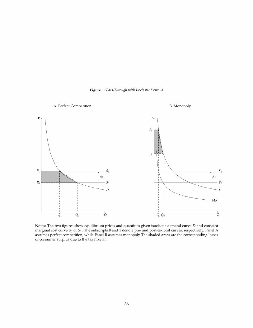
Figure 1: Pass-Through with Isoelastic Demand

P

Q

A. Perfect Competition

D

S0

S1

Q0Q1

P0

P1

dt

P

Q

B. Monopoly

D

MR

S0

S1

Q0Q1

P0

P1

dt

Notes: The two figures show equilibrium prices and quantities given isoelastic demand curve D and constantmarginal cost curve S0 or S1. The subscripts 0 and 1 denote pre- and post-tax cost curves, respectively. Panel Aassumes perfect competition, while Panel B assumes monopoly The shaded areas are the corresponding lossesof consumer surplus due to the tax hike dt.

36

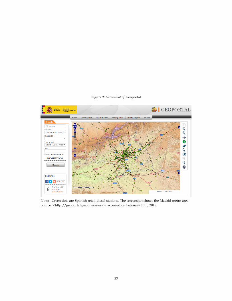
Figure 2: Screenshot of Geoportal

Notes: Green dots are Spanish retail diesel stations. The screenshot shows the Madrid metro area.Source: <http://geoportalgasolineras.es/>, accessed on February 15th, 2015.

37

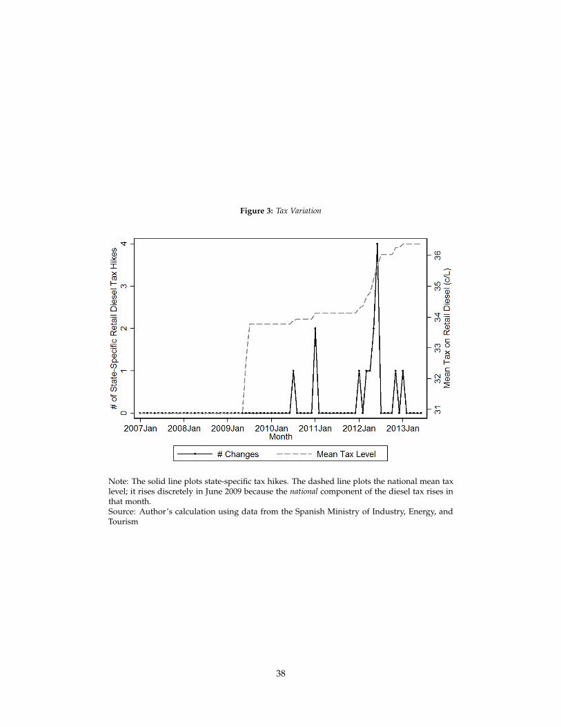
Figure 3: Tax Variation

Note: The solid line plots state-specific tax hikes. The dashed line plots the national mean taxlevel; it rises discretely in June 2009 because the national component of the diesel tax rises inthat month.Source: Author’s calculation using data from the Spanish Ministry of Industry, Energy, andTourism

38

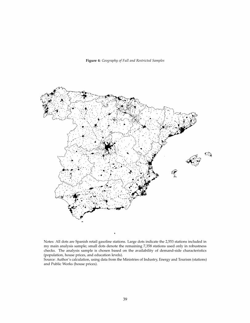
Figure 4: Geography of Full and Restricted Samples

Notes: All dots are Spanish retail gasoline stations. Large dots indicate the 2,553 stations included inmy main analysis sample; small dots denote the remaining 7,358 stations used only in robustnesschecks. The analysis sample is chosen based on the availability of demand-side characteristics(population, house prices, and education levels).Source: Author’s calculation, using data from the Ministries of Industry, Energy and Tourism (stations)and Public Works (house prices).

39

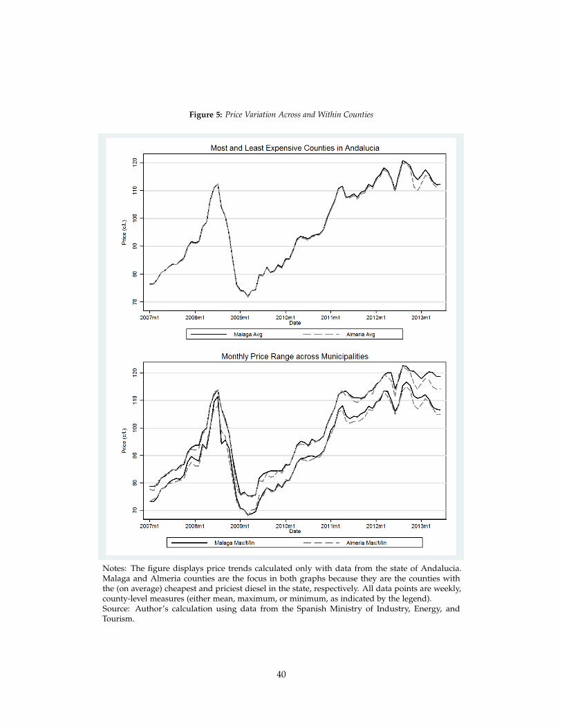
Figure 5: Price Variation Across and Within Counties

Notes: The figure displays price trends calculated only with data from the state of Andalucia.Malaga and Almeria counties are the focus in both graphs because they are the counties withthe (on average) cheapest and priciest diesel in the state, respectively. All data points are weekly,county-level measures (either mean, maximum, or minimum, as indicated by the legend).Source: Author’s calculation using data from the Spanish Ministry of Industry, Energy, andTourism.

40

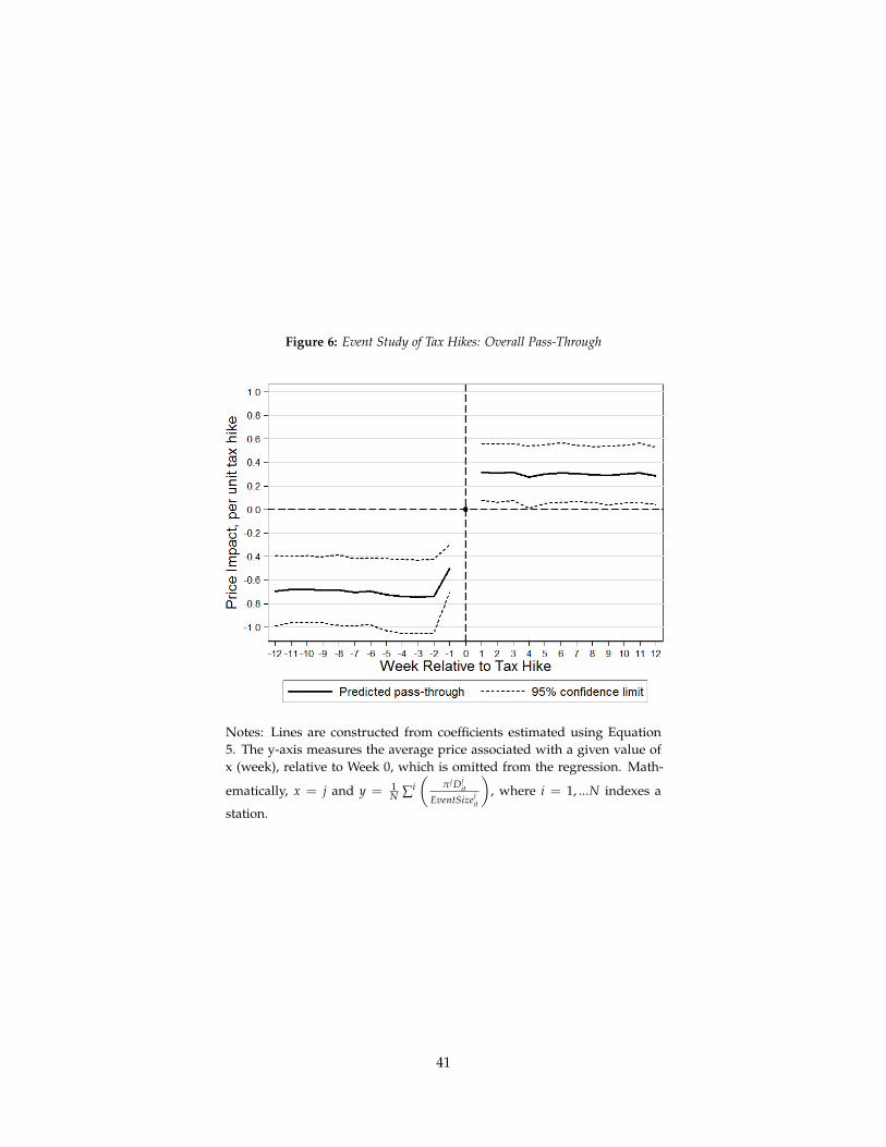
Figure 6: Event Study of Tax Hikes: Overall Pass-Through

Notes: Lines are constructed from coefficients estimated using Equation5. The y-axis measures the average price associated with a given value ofx (week), relative to Week 0, which is omitted from the regression. Math-

ematically, x = j and y = 1N ∑i

(π j Dj

it

EventSizejit

), where i = 1, ...N indexes a

station.

41

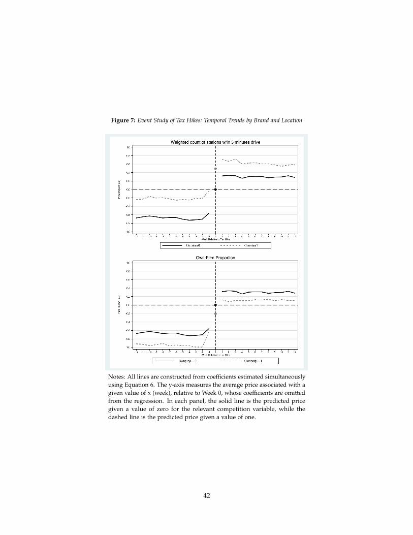
Figure 7: Event Study of Tax Hikes: Temporal Trends by Brand and Location

Notes: All lines are constructed from coefficients estimated simultaneouslyusing Equation 6. The y-axis measures the average price associated with agiven value of x (week), relative to Week 0, whose coefficients are omittedfrom the regression. In each panel, the solid line is the predicted pricegiven a value of zero for the relevant competition variable, while thedashed line is the predicted price given a value of one.

42

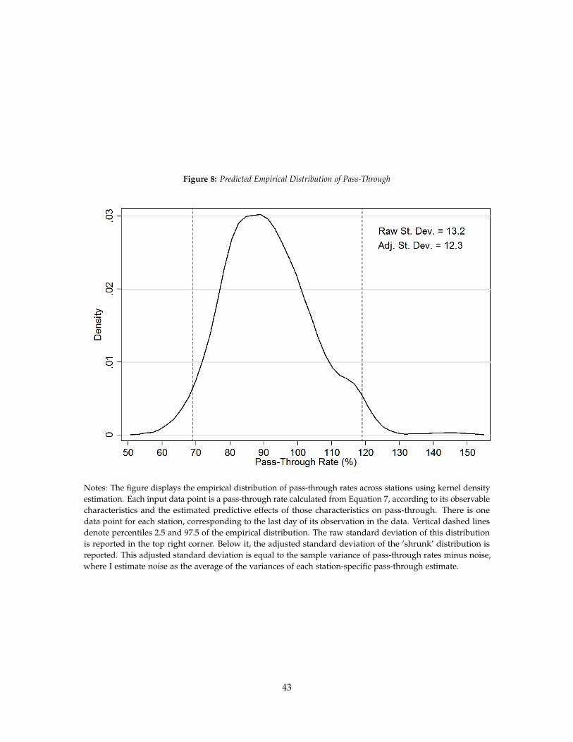
Figure 8: Predicted Empirical Distribution of Pass-Through

Notes: The figure displays the empirical distribution of pass-through rates across stations using kernel densityestimation. Each input data point is a pass-through rate calculated from Equation 7, according to its observablecharacteristics and the estimated predictive effects of those characteristics on pass-through. There is onedata point for each station, corresponding to the last day of its observation in the data. Vertical dashed linesdenote percentiles 2.5 and 97.5 of the empirical distribution. The raw standard deviation of this distributionis reported in the top right corner. Below it, the adjusted standard deviation of the ’shrunk’ distribution isreported. This adjusted standard deviation is equal to the sample variance of pass-through rates minus noise,where I estimate noise as the average of the variances of each station-specific pass-through estimate.

43

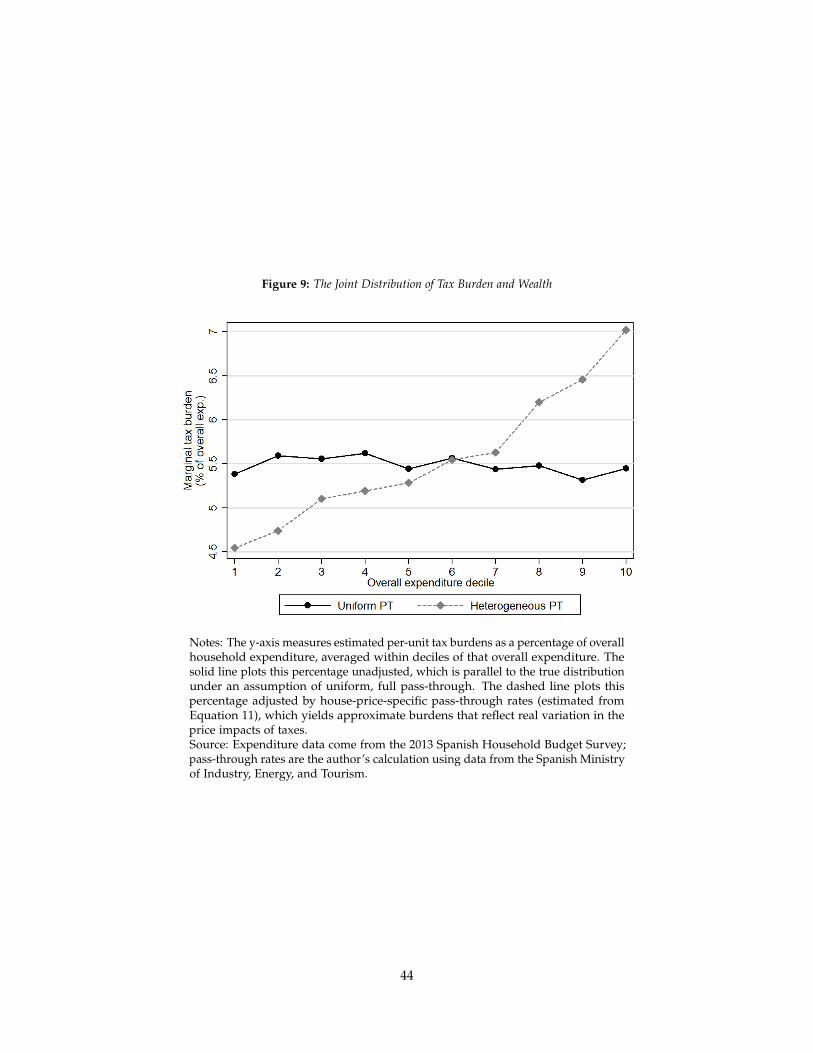
Figure 9: The Joint Distribution of Tax Burden and Wealth

Notes: The y-axis measures estimated per-unit tax burdens as a percentage of overallhousehold expenditure, averaged within deciles of that overall expenditure. Thesolid line plots this percentage unadjusted, which is parallel to the true distributionunder an assumption of uniform, full pass-through. The dashed line plots thispercentage adjusted by house-price-specific pass-through rates (estimated fromEquation 11), which yields approximate burdens that reflect real variation in theprice impacts of taxes.Source: Expenditure data come from the 2013 Spanish Household Budget Survey;pass-through rates are the author’s calculation using data from the Spanish Ministryof Industry, Energy, and Tourism.

44

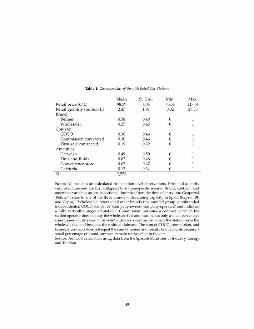
Table 1: Characteristics of Spanish Retail Gas Stations

Mean St. Dev. Min. Max.Retail price (c/L) 98.59 4.84 73.54 117.64Retail quantity (million L) 2.47 1.91 0.02 29.55Brand

Refiner 0.58 0.49 0 1Wholesaler 0.27 0.45 0 1

ContractCOCO 0.30 0.46 0 1Commission contracted 0.30 0.46 0 1Firm-sale contracted 0.19 0.39 0 1

AmenitiesCarwash 0.49 0.50 0 1Tires and fluids 0.63 0.48 0 1Convenience store 0.67 0.47 0 1Cafeteria 0.13 0.34 0 1

N 2,553

Notes: All statistics are calculated from station-level observations. Price and quantityvary over time and are first collapsed to station-specific means. Brand, contract, andamenities variables are cross-sectional dummies from the time of entry into Geoportal.’Refiner’ refers to any of the three brands with refining capacity in Spain (Repsol, BP,and Cepsa). ’Wholesaler’ refers to all other brands (the omitted group is unbrandedindependents). COCO stands for ’Company-owned, company-operated’ and indicatesa fully vertically-integrated station. ’Commission’ indicates a contract in which thestation operator does not buy the wholesale fuel and thus makes only a small percentagecommission on its sales. ’Firm-sale’ indicates a contract in which the station buys thewholesale fuel and becomes the residual claimant. The sum of COCO, commission, andfirm-sale contracts does not equal the sum of refiner and retailer brand counts because asmall percentage of brand contracts remain unclassified in the data.Source: Author’s calculation using data from the Spanish Ministries of Industry, Energy,and Tourism.

45

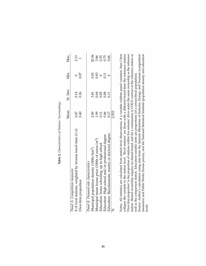
Tabl

e2:

Cha

ract

eris

tics

ofSt

atio

ns’S

urro

undi

ngs

Mea

nSt

.Dev

.M

in.

Max

.Pa

nelA

.Com

petit

ion

mea

sure

s#

ofri

vals

tati

ons,

wei

ghte

dby

inve

rse

trav

elti

me

(1/s

)0.

470.

140

2.13

Ow

n-fir

mpr

opor

tion

0.40

0.26

0.07

1

Pane

lB.D

eman

d-si

dech

arac

teri

stic

sM

unic

ipal

popu

lati

onde

nsit

y(1

000s

/km

2 )2.

893.

810.

0320

.56

Mun

icip

alm

ean

hous

epr

ice

(100

0sof

euro

s/m

2 )1.

990.

640.

833.

86Ed

ucat

ion:

Som

esc

hool

ing,

upto

high

scho

ol0.

110.

050

0.35

Educ

atio

n:H

igh

scho

olan

d/or

prof

essi

onal

degr

ee0.

460.

080.

110.

75Ed

ucat

ion:

Bacc

alau

reat

e,m

aste

r,or

doct

oral

degr

ee0.

170.

110

0.66

N2,

553

Not

es:

All

stat

isti

csar

eca

lcu

late

dfr

omst

atio

n-le

vel

obse

rvat

ions

;if

ava

riab

leex

hibi

tsp

anel

vari

atio

n,th

enI

firs

tco

llap

seth

eva

riab

leto

the

stat

ion

leve

l.’R

ival

stat

ions

’are

thos

ew

ith

ad

iffe

rent

bran

dth

anth

ere

fere

nce

stat

ion.

’Ow

n-fir

mpr

opor

tion’

isth

epr

opor

tion

ofst

atio

nsw

ithin

five

min

utes

’dri

veun

der

the

sam

eow

ners

hip

asth

ere

fere

nce

stat

ion.

Shar

edow

ners

hip

requ

ires

(a)s

hare

dbr

and,

and

(b)a

com

mis

sion

orC

OC

Oco

ntra

ctat

the

refe

renc

est

atio

nas

wel

las

the

com

pari

son

stat

ion.

Educ

atio

n-va

riab

leun

its

are

prop

orti

ons

(of

ace

nsus

-blo

ckpo

pula

tion

).So

urc

e:A

uth

or’s

calc

ula

tion

usi

ngd

ata

from

the

Span

ish

Min

istr

ies

ofIn

du

stry

,Ene

rgy,

and

Tou

rism

(com

pet

itio

nm

easu

res)

and

Pu

blic

Wor

ks(h

ouse

pric

es),

and

the

Nat

iona

lSta

tist

ical

Inst

itu

te(p

opu

lati

ond

ensi

tyan

ded

uca

tion

leve

l).

46

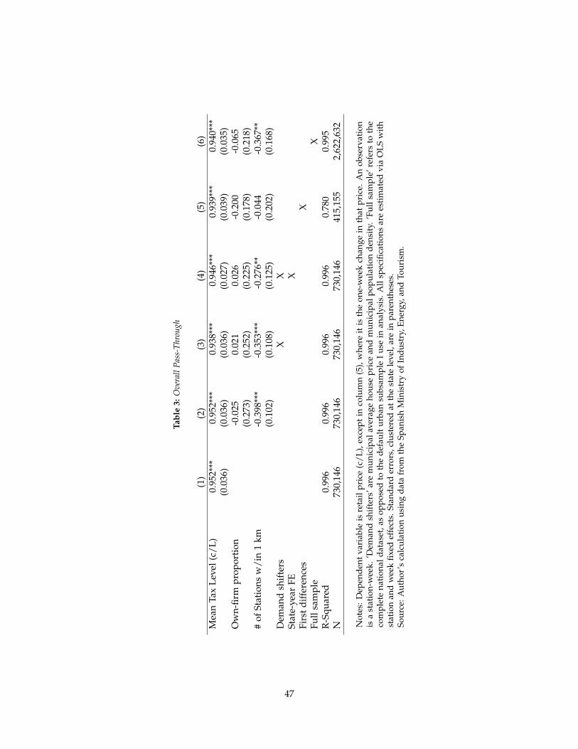
Tabl

e3:

Ove

rall

Pass

-Thr

ough

(1)

(2)

(3)

(4)

(5)

(6)

Mea

nTa

xLe

vel(

c/L)

0.95

2***

0.95

2***

0.93

8***

0.94

6***

0.93

9***

0.94

0***

(0.0

36)

(0.0

36)

(0.0

36)

(0.0

27)

(0.0

39)

(0.0

35)

Ow

n-fir

mpr

opor

tion

-0.0

250.

021

0.02

6-0

.200

-0.0

65(0

.273

)(0

.252

)(0

.225

)(0

.178

)(0

.218

)#

ofSt

atio

nsw

/in

1km

-0.3

98**

*-0

.353

***

-0.2

76**

-0.0

44-0

.367

**(0

.102

)(0

.108

)(0

.125

)(0

.202

)(0

.168

)D

eman

dsh

ifte

rsX

XSt

ate-

year

FEX

Firs

tdi

ffer

ence

sX

Full

sam

ple

XR

-Squ

ared

0.99

60.

996

0.99

60.

996

0.78

00.

995

N73

0,14

673

0,14

673

0,14

673

0,14

641

5,15

52,

622,

632

Not

es:

Dep

end

ent

vari

able

isre

tail

pri

ce(c

/L

),ex

cep

tin

colu

mn

(5),

whe

reit

isth

eon

e-w

eek

chan

gein

that

pri

ce.

An

obse

rvat

ion

isa

stat

ion-

wee

k.’D

eman

dsh

ifte

rs’a

rem

unic

ipal

aver

age

hous

epr

ice

and

mun

icip

alpo

pula

tion

den

sity

.’F

ulls

ampl

e’re

fers

toth

eco

mpl

ete

nati

onal

dat

aset

,as

oppo

sed

toth

ed

efau

ltur

ban

subs

ampl

eI

use

inan

alys

is.A

llsp

ecifi

cati

ons

are

esti

mat

edvi

aO

LS

wit

hst

atio

nan

dw

eek

fixed

effe

cts.

Stan

dard

erro

rs,c

lust

ered

atth

est

ate

leve

l,ar

ein

pare

nthe

ses.

Sour

ce:A

utho

r’s

calc

ulat

ion

usin

gda

tafr

omth

eSp

anis

hM

inis

try

ofIn

dust

ry,E

nerg

y,an

dTo

uris

m.

47

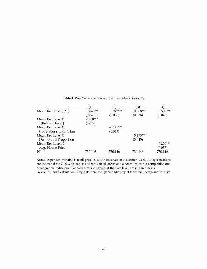
Table 4: Pass-Through and Competition: Each Metric Separately

(1) (2) (3) (4)Mean Tax Level (c/L) 0.845*** 0.943*** 0.868*** 0.598***

(0.046) (0.036) (0.036) (0.076)Mean Tax Level X 0.138***

1[Refiner Brand] (0.029)Mean Tax Level X -0.117***

# of Stations w/in 1 km (0.035)Mean Tax Level X 0.173***

Own-Brand Proportion (0.045)Mean Tax Level X 0.220***

Avg. House Price (0.037)N 730,146 730,146 730,146 730,146

Notes: Dependent variable is retail price (c/L). An observation is a station-week. All specificationsare estimated via OLS with station and week fixed effects and a control vector of competition anddemographic indicators. Standard errors, clustered at the state level, are in parentheses.Source: Author’s calculation using data from the Spanish Ministry of Industry, Energy, and Tourism.

48

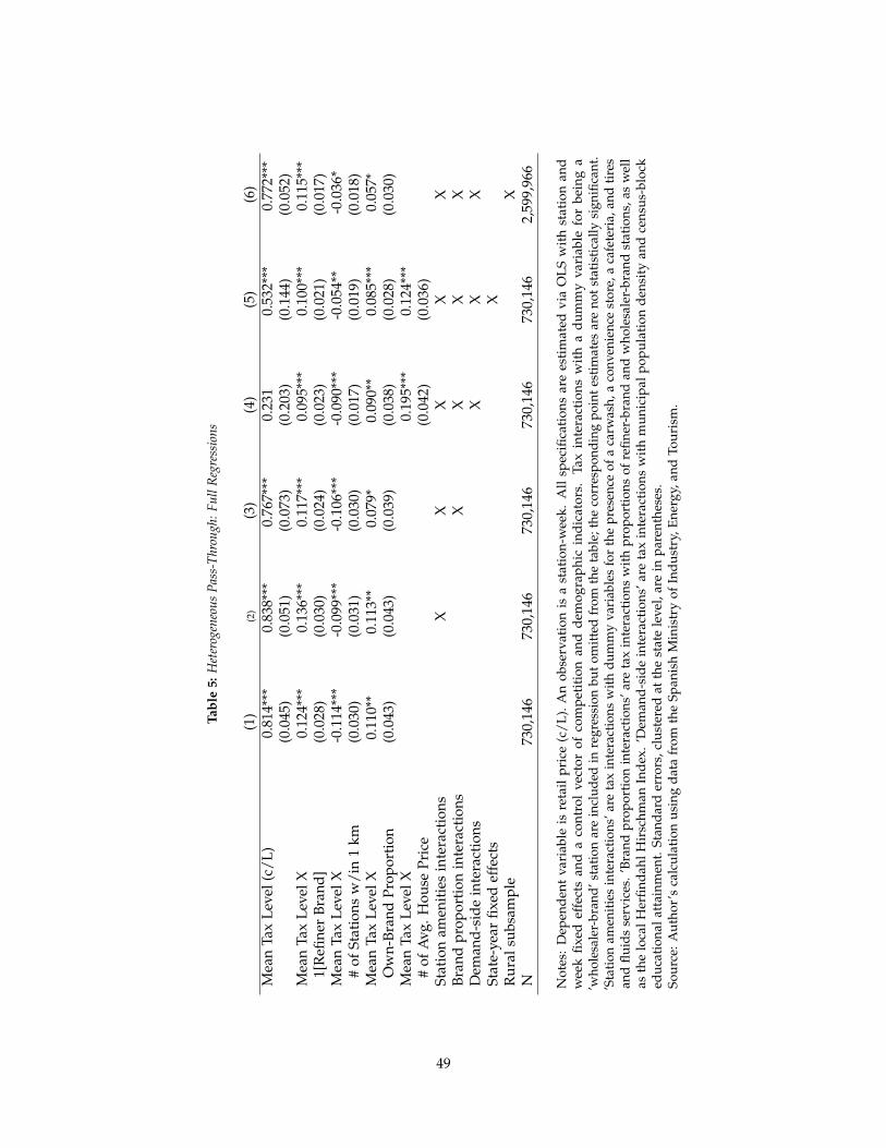
Tabl

e5:

Het

erog

eneo

usPa

ss-T

hrou

gh:F

ullR

egre

ssio

ns

(1)

(2)

(3)

(4)

(5)

(6)

Mea

nTa

xLe

vel(

c/L)

0.81

4***

0.83

8***

0.76

7***

0.23

10.

532*

**0.

772*

**(0

.045

)(0

.051

)(0

.073

)(0

.203

)(0

.144

)(0

.052

)M

ean

Tax

Leve

lX0.

124*

**0.

136*

**0.

117*

**0.

095*

**0.

100*

**0.

115*

**1[

Refi

ner

Bran

d](0

.028

)(0

.030

)(0

.024

)(0

.023

)(0

.021

)(0

.017

)M

ean

Tax

Leve

lX-0

.114

***

-0.0

99**

*-0

.106

***

-0.0

90**

*-0

.054

**-0

.036

*#

ofSt

atio

nsw

/in

1km

(0.0

30)

(0.0

31)

(0.0

30)

(0.0

17)

(0.0

19)

(0.0

18)

Mea

nTa

xLe

velX

0.11

0**

0.11

3**

0.07

9*0.

090*

*0.

085*

**0.

057*

Ow

n-Br

and

Prop

orti

on(0

.043

)(0

.043

)(0

.039

)(0

.038

)(0

.028

)(0

.030

)M

ean

Tax

Leve

lX0.

195*

**0.

124*

**#

ofA

vg.H

ouse

Pric

e(0

.042

)(0

.036

)St

atio

nam

enit

ies

inte

ract

ions

XX

XX

XBr

and

prop

orti

onin

tera

ctio

nsX

XX

XD

eman

d-si

dein

tera

ctio

nsX

XX

Stat

e-ye

arfix

edef

fect

sX

Rur

alsu

bsam

ple

XN

730,

146

730,

146

730,

146

730,

146

730,

146

2,59

9,96

6

Not

es:

Dep

end

ent

vari

able

isre

tail

pri

ce(c

/L

).A

nob

serv

atio

nis

ast

atio

n-w

eek.

All

spec

ifica

tion

sar

ees

tim

ated

via

OL

Sw

ith

stat

ion

and

wee

kfi

xed

effe

cts

and

aco

ntro

lve

ctor

ofco

mp

etit

ion

and

dem

ogra

phi

cin

dic

ator

s.Ta

xin

tera

ctio

nsw

ith

ad

um

my

vari

able

for

bein

ga

’who

lesa

ler-

bran

d’st

atio

nar

ein

clud

edin

regr

essi

onbu

tom

itted

from

the

tabl

e;th

eco

rres

pond

ing

poin

test

imat

esar

eno

tsta

tistic

ally

sign

ifica

nt.

’Sta

tion

amen

ities

inte

ract

ions

’are

tax

inte

ract

ions

with

dum

my

vari

able

sfo

rth

epr

esen

ceof

aca

rwas

h,a

conv

enie

nce

stor

e,a

cafe

teri

a,an

dtir

esan

dflu

ids

serv

ices

.’Br

and

prop

orti

onin

tera

ctio

ns’a

reta

xin

tera

ctio

nsw

ith

prop

orti

ons

ofre

finer

-bra

ndan

dw

hole

sale

r-br

and

stat

ions

,as

wel

las

the

loca

lHer

find

ahlH

irsc

hman

Ind

ex.

’Dem

and

-sid

ein

tera

ctio

ns’a

reta

xin

tera

ctio

nsw

ith

mun

icip

alpo

pula

tion

den

sity

and

cens

us-b

lock

educ

atio

nala

ttai

nmen

t.St

anda

rder

rors

,clu

ster

edat

the

stat

ele

vel,

are

inpa

rent

hese

s.So

urce

:Aut

hor’

sca

lcul

atio

nus

ing

data

from

the

Span

ish

Min

istr

yof

Indu

stry

,Ene

rgy,

and

Tour

ism

.

49

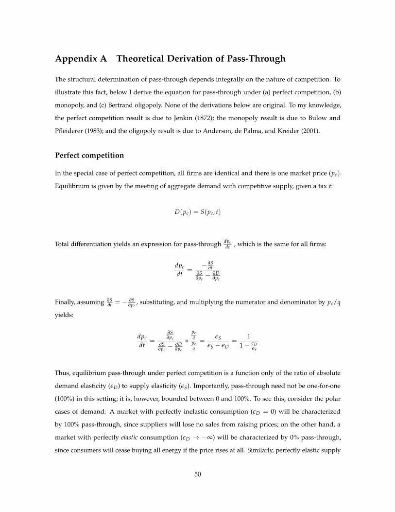
Appendix A Theoretical Derivation of Pass-Through

The structural determination of pass-through depends integrally on the nature of competition. To

illustrate this fact, below I derive the equation for pass-through under (a) perfect competition, (b)

monopoly, and (c) Bertrand oligopoly. None of the derivations below are original. To my knowledge,

the perfect competition result is due to Jenkin (1872); the monopoly result is due to Bulow and

Pfleiderer (1983); and the oligopoly result is due to Anderson, de Palma, and Kreider (2001).

Perfect competition

In the special case of perfect competition, all firms are identical and there is one market price (pc).

Equilibrium is given by the meeting of aggregate demand with competitive supply, given a tax t:

D(pc) = S(pc, t)

Total differentiation yields an expression for pass-through dpcdt , which is the same for all firms:

dpc

dt=

− ∂S∂t

∂S∂pc− ∂D

∂pc

Finally, assuming ∂S∂t = − ∂S

∂pc, substituting, and multiplying the numerator and denominator by pc/q

yields:

dpc

dt=

∂S∂pc

∂S∂pc− ∂D

∂pc

∗pcqpcq

=εS

εS − εD=

11− εD

εS

Thus, equilibrium pass-through under perfect competition is a function only of the ratio of absolute

demand elasticity (εD) to supply elasticity (εS). Importantly, pass-through need not be one-for-one

(100%) in this setting; it is, however, bounded between 0 and 100%. To see this, consider the polar

cases of demand: A market with perfectly inelastic consumption (εD = 0) will be characterized

by 100% pass-through, since suppliers will lose no sales from raising prices; on the other hand, a

market with perfectly elastic consumption (εD → −∞) will be characterized by 0% pass-through,

since consumers will cease buying all energy if the price rises at all. Similarly, perfectly elastic supply

50

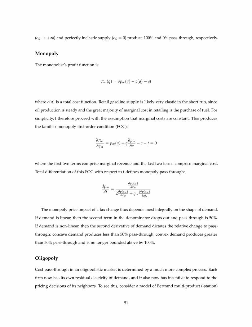
(εS → +∞) and perfectly inelastic supply (εS = 0) produce 100% and 0% pass-through, respectively.

Monopoly

The monopolist’s profit function is:

πm(q) = qpm(q)− c(q)− qt

where c(q) is a total cost function. Retail gasoline supply is likely very elastic in the short run, since

oil production is steady and the great majority of marginal cost in retailing is the purchase of fuel. For

simplicity, I therefore proceed with the assumption that marginal costs are constant. This produces

the familiar monopoly first-order condition (FOC):

∂πm

∂qm= pm(q) + q

∂pm

∂q− c− t = 0

where the first two terms comprise marginal revenue and the last two terms comprise marginal cost.

Total differentiation of this FOC with respect to t defines monopoly pass-through:

dpm

dt=

∂p(qm)∂qm

2 ∂p(qm)∂qm

+ qm∂2 p(qm)

∂q2m

The monopoly price impact of a tax change thus depends most integrally on the shape of demand.

If demand is linear, then the second term in the denominator drops out and pass-through is 50%.

If demand is non-linear, then the second derivative of demand dictates the relative change to pass-

through: concave demand produces less than 50% pass-through; convex demand produces greater

than 50% pass-through and is no longer bounded above by 100%.

Oligopoly

Cost pass-through in an oligopolistic market is determined by a much more complex process. Each

firm now has its own residual elasticity of demand, and it also now has incentive to respond to the

pricing decisions of its neighbors. To see this, consider a model of Bertrand multi-product (-station)

51

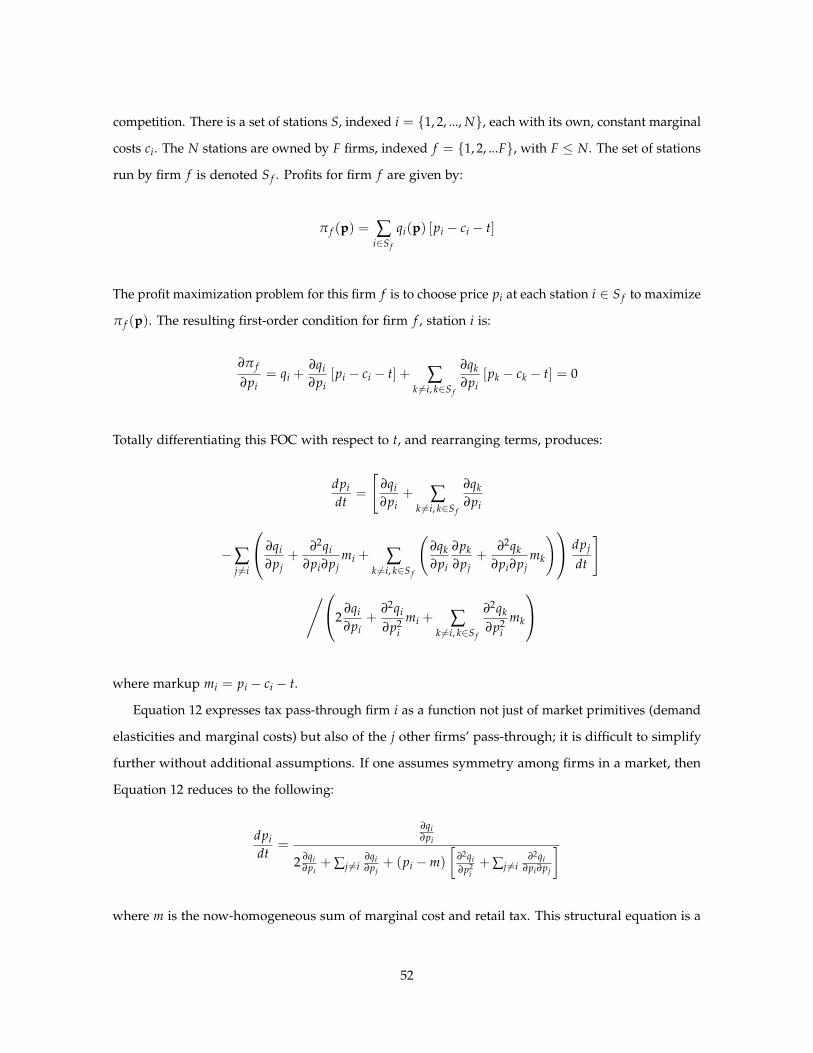
competition. There is a set of stations S, indexed i = {1, 2, ..., N}, each with its own, constant marginal

costs ci. The N stations are owned by F firms, indexed f = {1, 2, ...F}, with F ≤ N. The set of stations

run by firm f is denoted S f . Profits for firm f are given by:

π f (p) = ∑i∈S f

qi(p) [pi − ci − t]

The profit maximization problem for this firm f is to choose price pi at each station i ∈ S f to maximize

π f (p). The resulting first-order condition for firm f , station i is:

∂π f

∂pi= qi +

∂qi∂pi

[pi − ci − t] + ∑k 6=i, k∈S f

∂qk∂pi

[pk − ck − t] = 0

Totally differentiating this FOC with respect to t, and rearranging terms, produces:

dpidt

=

[∂qi∂pi

+ ∑k 6=i, k∈S f

∂qk∂pi

−∑j 6=i

∂qi∂pj

+∂2qi

∂pi∂pjmi + ∑

k 6=i, k∈S f

(∂qk∂pi

∂pk∂pj

+∂2qk

∂pi∂pjmk

) dpj

dt

]

/2∂qi∂pi

+∂2qi

∂p2i

mi + ∑k 6=i, k∈S f

∂2qk

∂p2i

mk

where markup mi = pi − ci − t.

Equation 12 expresses tax pass-through firm i as a function not just of market primitives (demand

elasticities and marginal costs) but also of the j other firms’ pass-through; it is difficult to simplify

further without additional assumptions. If one assumes symmetry among firms in a market, then

Equation 12 reduces to the following:

dpidt

=

∂qi∂pi

2 ∂qi∂pi

+ ∑j 6=i∂qi∂pj

+ (pi −m)

[∂2qi∂p2

i+ ∑j 6=i

∂2qi∂pi∂pj

]

where m is the now-homogeneous sum of marginal cost and retail tax. This structural equation is a

52

generalized version of Equation 12, which defines monopoly pass-through - if there were no other

firms j in the market, Equation 12 would collapse back down to Equation 12. Just as in the monopoly

case, both first and second derivatives of demand matter in oligopoly. However, other stations now

affect the decision of station i. Its pass-through rate is now additionally a function of the cross-price

elasticities ∂qi∂pj

as well the cross-price derivatives of own-price elasticities ∑j 6=i∂2qi

∂pi∂pj.

53