NBER WORKING PAPER SERIES

WHO BENEFITS FROM STATE CORPORATE TAX CUTS? A LOCAL LABOR MARKETS APPROACH WITH HETEROGENEOUS FIRMS

Juan Carlos Suárez SerratoOwen Zidar

Working Paper 20289http://www.nber.org/papers/w20289

NATIONAL BUREAU OF ECONOMIC RESEARCH1050 Massachusetts Avenue

Cambridge, MA 02138

We are very grateful for guidance and support from our advisors: Alan Auerbach, Yuriy Gorodnichenko, Patrick Kline, and Emmanuel Saez. We would like to thank the Editor Luigi Pistaferri and three anonymous referees for their helpful comments. We are also indebted to David Albouy, Dominick Bartelme, Alex Bartik, Pat Bayer, Michael Boskin, Eric Budish, David Card, Jeffrey Clemens, Robert Chirinko, Rebecca Diamond, Jonathan Dingel, Pascaline Dupas, Matt Gentzkow, Gopi Goda, Marc Hafstead, Jim Hines, Caroline Hoxby, Erik Hurst, Koichiro Ito, Matt Leister, Attila Lindner, Neale Mahoney, John McClelland, David Molitor, Enrico Moretti, Pascal Noel, Matt Notowidigdo, Alexandre Poirier, Jim Poterba, Andrés Rodríguez-Clare, Jesse Rothstein, Greg Rosston, Florian Scheuer, John Shoven, Orie Shelef, Reed Walker, Dan Wilson, Danny Yagan, Shuang Zhang, and Eric Zwick for helpful comments and suggestions. We are especially thankful to Nathan Seegert, Dan Wilson and Robert Chirinko, and Jamie Bernthal, Dana Gavrila, Katie Schumacher, Shane Spencer, and Katherine Sydor for generously providing us with tax data. Tim Anderson, Anastasia Bogdanova, Pawel Charasz, Stephen Lamb, Matt Panhans, Prab Upadrashta, John Wieselthier, and Victor Ye provided excellent research assistance. All errors remain our own. This work is supported by the Kauffman Foundation and the Kathryn and Grant Swick Faculty Research Fund at the University of Chicago Booth School of Business. We declare that we have no relevant or material financial interests that relate to the research described in this paper. The views expressed herein are those of the authors and do not necessarily reflect the views of the National Bureau of Economic Research.

NBER working papers are circulated for discussion and comment purposes. They have not been peer-reviewed or been subject to the review by the NBER Board of Directors that accompanies official NBER publications.

© 2014 by Juan Carlos Suárez Serrato and Owen Zidar. All rights reserved. Short sections of text, not to exceed two paragraphs, may be quoted without explicit permission provided that full credit, including © notice, is given to the source.

Who Benefits from State Corporate Tax Cuts? A Local Labor Markets Approach with Heterogeneous FirmsJuan Carlos Suárez Serrato and Owen ZidarNBER Working Paper No. 20289July 2014, Revised August 2016JEL No. F22,F23,H2,H22,H25,H32,H71,J23,J3,R23,R30,R58

ABSTRACT

This paper estimates the incidence of state corporate taxes on the welfare of workers, landowners,and firm owners using variation in state corporate tax rates and apportionment rules. We develop aspatial equilibrium model with imperfectly mobile firms and workers. Firm owners may earn profitsand be inframarginal in their location choices due to differences in location-specific productivities.We use the reduced-form effects of tax changes to identify and estimate incidence as well as the structuralparameters governing these impacts. In contrast to standard open economy models, firm owners bearroughly 40% of the incidence, while workers and landowners bear 30-35% and 25-30%, respectively.

Juan Carlos Suárez SerratoDepartment of EconomicsDuke University213 Social Sciences BuildingBox 90097Durham, NC 27708and NBERjc@jcsuarez.com

Owen ZidarUniversity of ChicagoBooth School of Business5807 South Woodlawn AvenueChicago, IL 60637and NBERowen.zidar@chicagobooth.edu

This paper evaluates the welfare e↵ects of corporate income tax cuts on business owners, workers,

and landowners. The conventional wisdom among economists and policymakers is that corporate tax-

ation in an open economy is unattractive on both e�ciency and equity grounds: it distorts the location

and scale of economic activity and falls on the shoulders of workers.1 We revisit this conventional

wisdom both empirically and theoretically.

We begin by developing a spatial equilibrium model in which firm productivity and profitability

can di↵er across locations.2 Standard models without these features have a di�cult time explaining

how California, with corporate tax rates of nearly 10%, is home to one out of nine establishments in

the United States, especially when neighboring Nevada has no corporate tax. Our modeling approach

acknowledges that if California were to increase corporate tax rates modestly, many new and existing

technology firms would continue to find Silicon Valley to be the most profitable location in the world.

The presence of such inframarginal firms changes the nature of the equity and e�ciency tradeo↵ by

allowing firms (and their shareholders) to bear some of the incidence associated with corporate taxes.3

We implement this model empirically to provide a new assessment of the welfare e↵ects of local

corporate tax cuts. The welfare e↵ects are point identified by the reduced-form impacts of changes in

business taxes on four outcomes: wages, rental costs, the location decisions of establishments, and the

location decisions of workers. We estimate these impacts using variation in state corporate tax rates

and rules and establish their validity through a number of tests. These reduced-form impacts enable

us to estimate the welfare e↵ects of state corporate tax cuts as well as the structural parameters

that rationalize these e↵ects. The structural parameters are similar to existing estimates from the

literature, to the extent these estimates exist.

We have two main results. First, we unambiguously reject the conventional view of 100% inci-

dence on workers and 0% on firm owners based on a variety of approaches: reduced-form estimates,

structural estimates, and calibrations using existing estimates from the local labor markets literature.

Second, our baseline estimates place approximately 40% of the burden on firm owners, 25-30% on

landowners and 30-35% on workers. The result that firm owners may bear the incidence of local poli-

cies starkly contrasts with existing results in the corporate tax literature (e.g., Fullerton and Metcalf

(2002)) and is a novel result in the local labor markets literature (e.g., Moretti (2011)).

We establish these results in three steps. In the first part of the paper, we construct the model

to allow for the possibility that firm owners, workers, and landowners can bear incidence. The

incidence on these three groups depends on the equilibrium impacts on profits, real wages, and

housing costs, respectively. A tax cut mechanically reduces the tax liability and the cost of capital

of local establishments, attracts establishments, and increases local labor demand. This increase in

labor demand leads firms to o↵er higher wages, encourages migration of workers, and increases the

1See for instance, Gordon and Hines (2002). Gravelle and Smetters (2006) and Arulampalam, Devereux and Ma�ni(2012) show how imperfect product substitution and wage bargaining, respectively, can alter this conclusion, and Desai,Foley and Hines Jr. (2007) find that labor bears the majority but not all of the burden internationally. Note that wefrequently use “tax cuts” as shorthand for “tax changes” since our main specifications use keep-rates.

2While many papers have documented large and persistent productivity di↵erences across countries (Hall and Jones,1999), sectors (Levchenko and Zhang, 2012), businesses (Syverson, 2011), and local labor markets (Moretti, 2011),the corporate tax literature has not accounted for the role that heterogeneous productivities may have in determiningequilibrium incidence. Some research on the incidence of local corporate tax cuts exists – for instance, Fuest, Peichl andSiegloch (2013) use employer-firm linked data to assess the e↵ects of corporate taxes on wages in Germany – but to ourknowledge, there are no empirical analyses that incorporate local equilibrium e↵ects of these tax changes. Interestingly,they also find similar results for the incidence on workers in their full sample specification.

3Existing and new firms can be inframarginal due to heterogeneous productivities. This idea is conceptually distinctfrom the taxation of “old” capital as discussed by Auerbach (2006). See Liu and Altshuler (2013) and Cronin et al.(2013) for incidence papers that allow for imperfect competition and supernormal economic profits, respectively.

1

cost of housing. Our model characterizes the new spatial equilibrium following a business tax cut and

relates the changes in wages, rents, and profits to a few key parameters governing labor, housing, and

product markets. In particular, the incidence on wages depends on the degree to which establishment

location decisions respond to tax changes, an e↵ective labor supply elasticity that is dependent on

housing market conditions, and a macro labor demand elasticity that depends on location and scale

decisions of establishments. Having determined the incidence on wages, the incidence on profits

is straightforward; it combines the mechanical e↵ects of lower corporate taxes and the impact of

higher wages on production costs and scale decisions. Finally, we show that the equilibrium incidence

formulae on worker welfare, firm profits, and landowners’ rents are identified by reduced-form e↵ects

of corporate taxes as well as by structural parameters of the model.

In the second part of the paper, the empirical analysis quantifies the responsiveness of local

economic activity to local business tax changes. The variation in our empirical analysis comes from

changes to state corporate tax rates and apportionment rules, which are state-specific rules that

govern how national profits of multi-state firms are allocated for tax purposes.4 We implement these

state corporate tax system rules using matched firm-establishment data and construct a measure of

the average tax rate that businesses pay in a local area. This approach not only closely approximates

actual taxes paid by businesses, but it also provides multiple sources of identifying variation from

changes in state tax rates, apportionment formulae, and the rate and rule changes of other states.

We find that a 1% cut in local business taxes increases the number of local establishments by 3 to

4% over a ten-year period. This estimate is unrelated to other changes in policy that would otherwise

bias our results, including changes in per-capita government spending and changes in the corporate

tax base such as investment tax credits. To rule out the possibility that business tax changes occur in

response to abnormal economic conditions, we analyze the typical dynamics of establishment growth

in the years before and after business tax cuts. We also directly control for a common measure of

changes in local labor demand from Bartik (1991). Finally, we estimate the e↵ects of external tax

changes of other locations on local establishment growth and find symmetric e↵ects of business tax

changes on establishment growth. These symmetric e↵ects corroborate the robustness of our reduced-

form results of business tax changes. We also provide estimates of the e↵ects of corporate tax cuts

on local population, wages, and rental costs.

In the third part of the paper, we use these reduced-form results to estimate the incidence of busi-

ness tax changes. We first apply the incidence expressions that transparently map four reduced-form

e↵ects – on business and worker location, wages, and rental costs – to the welfare e↵ects on workers,

landowners, and firm owners. We then estimate the structural parameters governing incidence by

minimizing the distance between the four reduced-form e↵ects and their theoretical counterparts. We

test over-identifying restrictions of the model and find that they are satisfied. The structural elastic-

ities are precisely estimated. These elasticities help reinforce the validity of our overall estimates for

two reasons. First, our estimated elasticities align with existing estimates from the literature. Second,

they enable us to use estimates from Suarez Serrato and Wingender (2011) to show that our results

are robust and, if anything, modestly strengthened when accounting for the welfare e↵ects of changes

in government spending that result from changes in tax revenue. Government service reductions

disproportionately hurt workers and infrastructure reductions hurt both firms and workers; lower

4Previous studies have focused on the theoretical distortions that apportionment formulae have on the geographicallocation of capital and labor (see, e.g., McLure Jr. (1982) and Gordon and Wilson (1986)). Empirically, several studieshave used variation in apportionment rules (e.g., Goolsbee and Maydew (2000)). Hines (2009) and Devereux and Loretz(2007) have analyzed how these tax distortions a↵ect the location of economic activity internationally.

2

infrastructure reduces productivity and thus wages. The magnitudes of these adjustments depend on

the magnitude of tax revenue changes, which can be small in practice due to low tax revenue shares

from corporate taxes and fiscal externalities on sales and individual income tax bases.

In the last section of the paper, we analyze the e�ciency costs of state corporate income taxes and

discuss the implications of our results for tax revenues and the revenue-maximizing tax rate. Although

business mobility is an often-cited justification in proposals to lower states’ corporate tax rates,

business location distortions per se do not lead to a low revenue-maximizing rate. Based solely on

the responsiveness of establishment location to tax changes, corporate tax revenue-maximizing rates

would be nearly 32%. This rate greatly exceeds average state corporate tax rates, which were 7% on

average in 2010. However, corporate tax cuts have large fiscal externalities by distorting the location

of individuals. This additional consideration implies substantially lower revenue-maximizing state

corporate tax rates than 32%. The revenue-maximizing tax rate also depends on state apportionment

rules. By apportioning on the basis of sales activity, policymakers can decrease the importance of

firms’ location decisions in the determination of their tax liabilities and thus lower the distortionary

e↵ects of corporate taxes. Overall, accounting for fiscal externalities and apportionment results in

revenue-maximizing rates that are close to actual statutory rates on average.

This paper contributes a new assessment of the incidence of corporate taxation. The existing

corporate tax literature provides a wide range of conclusions about the corporate tax burden. In

the seminal paper of this literature, Harberger (1962) finds that under reasonable parameter values,

capital bears the burden of a tax in a closed economy model in which all the adjustment has to

be through factor prices. However, di↵erent capital mobility assumptions can completely reverse

Harberger’s conclusion (Kotliko↵ and Summers, 1987). Gravelle (2010) shows how conclusions from

various studies hinge on their modeling assumptions, while Fullerton and Metcalf (2002) note that

“few of the standard assumptions about tax incidence have been tested and confirmed.” Gravelle

(2011) and Clausing (2013) critically review some of the existing empirical work on corporate tax

incidence. We contribute to both the theoretical and empirical corporate tax literature by developing

a new theoretical approach, which can accommodate the conventional view for hypothetical values of

the four reduced-form e↵ects, and by connecting this theory directly to the data. Doing so not only

allows the data to govern the relative mobility of firms and workers, but also enables us to conduct

inference on the resulting incidence calculations.

This paper also contributes to the recent local labor markets literature, which has focused on

the importance of linking workers and locations (Kline, 2010; Moretti, 2011; Suarez Serrato and

Wingender, 2011; Diamond, 2012; Busso, Gregory and Kline, 2013; Notowidigdo, 2013; Kline and

Moretti, 2013). This literature and benchmark models (Rosen, 1979; Roback, 1982; Glaeser, 2008)

have representative and perfectly competitive firms with no link between firms and location. Our work

links firms and locations by incorporating features popular in the trade literature (Krugman, 1979;

Hopenhayn, 1992; Melitz, 2003). Developing the demand side of local labor markets is important

because it allows for the possibility that firm owners can bear some of the incidence of local economic

development policies or local productivity shocks—a feature that was previously absent in models

of local labor markets.5 In addition, estimating labor demand functions in models of local labor

5One finding from the set of papers linking workers to locations that di↵erentiates them from previous work is thepossibility that workers may be inframarginal in their location decisions, which allows workers to bear the benefit or costof local policies. Our paper allows firms to be inframarginal in their location decisions. In addition, the possibility thatfirm owners can bear incidence implies that wage and property value responses alone are not su�cient for evaluating theincidence of productivity shocks and can alter the interpretation of existing work (e.g., Greenstone and Moretti (2004)).

3

markets has been limited by the lack of plausibly exogenous labor supply shocks that may trace

the slope of the demand function. Our framework exploits firm location decisions and the empirical

tradeo↵ firms make among productivity, corporate taxes, and factor prices to provide a novel link

between firm location choices and labor demand that can be used to recover the parameters governing

labor demand (and the incidence on firm profits). Finally, this paper relates to the literature on local

public finance and business location literatures.6 We contribute by providing a framework to interpret

existing estimates and by implementing the state corporate tax system, which provides novel variation.

We make several simplifying assumptions that may limit some of our analysis. First, we abstract

from issues of endogenous agglomerations or externalities that may result from changes in corporate

taxes. Second, we do not allow firms to bear the cost of rising real estate costs. This feature could

be added in a model with a real estate market that integrates the residential and commercial sectors.

However, given that firms’ cost shares on real estate are small, this addition would likely not change

our main result and would come at the cost of additional complexity. Third, our model abstracts

from the entrepreneurship margin (Gentry and Hubbard, 2000; Scheuer, 2014). Abstracting from

this margin is unlikely to a↵ect our incidence calculations to the extent that the entrepreneurship

margin is small. The magnitude of this margin depends on the e↵ect of one state’s tax changes on

the total number of businesses in the United States. Fourth, we compare steady states that assume

labor market clearing over a ten year period. Adding the possibility of unemployment during the

transition period could alter some of our conclusions about incidence.7 Fifth, many of the factors

in our incidence formulae are likely to be geographically heterogeneous. A more general model that

accounts for di↵erences in housing markets, sectoral compositions, and skill-group compositions as

well as non-linear housing supply functions may result in a better approximation to the incidence

in specific locations and in specific contexts. Sixth, while our cross-sectional approach provides

substantial variation, cross-sectional estimates necessarily abstract from general equilibrium e↵ects

that may a↵ect outcomes in all states.8 Finally, due to data limitations, we proxy for the benefit to

landowners using data on housing rents.

We proceed as follows. We develop the model in Section 1, derive simple expressions for incidence

in Section 2, and show how to estimate them in Section 3. Section 4 describes the data and U.S. state

corporate tax apportionment rules. Sections 5 and 6 provide reduced-form and structural results,

respectively. Section 7 discusses additional policy implications and Section 8 concludes.

6Important contributions include Gyourko and Tracy (1989); Bartik (1991); Haughwout and Inman (2001); Feldsteinand Vaillant (1998); Carlton (1983); Duranton, Gobillon and Overman (2011); Glaeser (2012); Hines (1997); Newman(1983); Bartik (1985); Helms (1985); Papke (1987, 1991); Goolsbee and Maydew (2000); Holmes (1998); Rothenberg(2012); Rathelot and Sillard (2008); Chirinko and Wilson (2008); Devereux and Gri�th (1998); Siegloch (2014); Hassettand Mathur (2015).

7More generally, we abstract from transition dynamics, which can have important incidence implications (Auerbach,2006). Interestingly, the benefits to firm owners are likely front-loaded as the mechanical e↵ects of tax cuts occurimmediately while the increases in wages and rental costs follow a gradual adjustment as establishments relocate.However, introducing unemployment into the model makes the welfare impacts during the transition harder to sign.

8If, for example, a tax change in Rhode Island a↵ects all wages nation-wide, our estimate would only report thedi↵erential e↵ect on Rhode Island versus other states and would subsume the aggregate e↵ect in the year fixed-e↵ect.However, to the extent that a single state’s taxes do not a↵ect the national level of wages, profits, and rental costs, ourestimates will provide the general equilibrium incidence.

4

1 A Spatial Equilibrium Model with Heterogeneous Firms

You have to start this conversation with the philosophy that businesses have more choices than theyever have before. And if you don’t believe that, you say taxes don’t matter. But if you do believe that,which I do, it’s one of those things, along with quality of life, quality of education, quality ofinfrastructure, cost of labor, it’s one of those things that matter.

—Delaware Governor Jack Markell (11/3/2013)

The model characterizes the incidence on wages, rents, and profits as functions of estimable parameters

governing the supply and demand sides of the housing, labor, and product markets. In particular, the

main incidence results will be functions of three key objects: the e↵ective elasticity of labor supply

"LS , the macro elasticity of labor demand "LD, and the increase in labor demand following a business

tax change @ lnLDc

@ ln(1�⌧bc ).

We consider a similar environment to Kline (2010) and Moretti (2011) in terms of worker location,

and develop the demand side of the local labor market by characterizing the location decisions of

heterogeneous firms. Specifically, we consider a small location c in an open economy with many other

locations. There are three types of agents: workers, establishment owners, and landowners. Units are

chosen so that the total number of workers N = 1 and establishments E = 1, and Nc and Ec denote

the share of workers and establishments in location c. The model is static and assumes no population

growth or establishment entry at the national level. Workers choose their location to maximize

utility, establishments choose location and scale to maximize after-tax profits, and landowners supply

housing units to maximize rental profits. In terms of market structure, capital and goods markets are

global and labor and housing markets are local. The equilibrium in location c is characterized by Nc

households earning wage wc and paying housing costs rc, Ec establishments earning after-tax profits

⇡c, and a representative landowner earning rents rc. We compare outcomes in spatial equilibrium

before and after a corporate tax cut and do not model the transition between pre-tax and post-tax

equilibria.

1.1 Household Problem

In location c with amenities A, households maximize Cobb-Douglas utility over housing h and a

composite X of non-housing goods xj while facing a wage w, rent r, and non-housing good prices pj :

maxh,X

lnA+ ↵ lnh+ (1� ↵) lnX s.t. rh+

Z

j2J

pjxjdj = w, where X =

0

B@Z

j2J

x"PD+1

"PD

j dj

1

CA

"PD

"PD+1

,

"PD < �1 is the product demand elasticity, and P is an elasticity of substitution (CES) price index

that is normalized to 1.9 Workers inelastically provide one unit of labor.

9The price index is defined as P =

R

j2J

(pj)1+"PD

dj

! 11+"PD

= 1. Demand from each household for variety j,

xj = (1�↵)wp"PD

j , depends on the non-housing expenditure, the price of variety j, and the product demand elasticity.

5

1.1.1 Household Location Choice

Wages, rental costs, and amenities vary across locations. The indirect utility of household n from

their choice of location c is then

V Wnc = a0 + lnwc � ↵ ln rc + lnAnc,

where a0 is a constant. Households maximize their indirect utility across locations, accounting for the

value of location-specific amenities lnAnc, which are comprised of a common location-specific term

Ac and location-specific idiosyncratic preference ⇠nc:10

maxc

a0 + lnwc � ↵ ln rc + Ac| {z }⌘uc

+⇠nc.

The presence of the household-specific-component allows for workers to be inframarginal in their

location choices and, in turn, allows for workers to bear part of the incidence of local shocks (Kline

and Moretti, 2013). Households will locate in location c if their indirect utility there is higher than

in any other location c0. Assuming ⇠0ncs are i.i.d. type I extreme value, the share of households for

whom that is true determines local population Nc:

Nc = P

✓V Wnc = max

c0{V W

nc0}◆

=exp uc

�WPc0 exp

uc0�W

, (1)

where �W is the dispersion of the location-specific idiosyncratic preference ⇠nc. This equation defines

the local labor supply as a function that is increasing in wages wc, decreasing in rents rc, and increasing

in log amenities Ac. If workers have similar tastes for cities, then �W will be low and local labor

supply will be fairly responsive to real wage and amenity changes.

1.2 Housing Market

Local housing demand follows from the household problem and is given by: HDc = Nc↵wc

rc. The

local supply of housing, HSc = G(rc;BH

c ), is upward-sloping in both the rental price rc, which al-

lows landowners to benefit from higher rental prices, and exogenous local housing productivity BHc .

The marginal landowner supplies housing at cost rc = G�1(HSc ;B

Hc ). For tractability, we assume

G(rc;BHc ) ⌘ (BH

c rc)⌘c , where the local housing supply elasticity ⌘c > 0 governs the strength of the

price response to changes in demand and productivity.11 The housing market clearing condition,

HSc = HD

c , determines the rents rc in location c and is given in log-form by the following expression:

ln rc =1

1 + ⌘clnNc +

1

1 + ⌘clnwc �

⌘c1 + ⌘c

BHc + a1, (2)

where a1 is a constant. Substituting this expression into Equation 1 yields an expression for labor

supply that does not depend on rc but that incorporates the housing market feedback into the e↵ective

labor supply. This substitution yields the first key elasticity – the e↵ective elasticity of labor supply.

@ lnLSc

@ lnwc=

✓1 + ⌘c � ↵

�W (1 + ⌘c) + ↵

◆⌘ "LS

10Note that location preferences and heterogenous mobility costs, which some prior work (e.g., Topel (1986)) hasincluded, are observationally equivalent here. We assume fixed amenities for simplicity. See Diamond (2012) for ananalysis with endogenous amenities and Suarez Serrato and Wingender (2011) for an analysis where government servicesresponds to local population. We use estimates from Suarez Serrato and Wingender (2011) to quantify how our resultschange if government amenities are a↵ected in Appendix Section F.

11Note that we abstract from asymmetric housing supply; Notowidigdo (2013) discusses the incidence implications ofnon-linear housing supply as in Glaeser and Gyourko (2005).

6

1.3 Establishment Problem

The standard local labor markets and corporate tax models do not incorporate individual estab-

lishment location decisions. We add establishment location decisions for two main reasons. Firms’

location decisions enable us to identify the e↵ects of local tax changes on the prices and after-tax

profits of firm owners. They also provide a micro-foundation for the local labor demand elasticity

based on firms’ location and scale decisions.

Establishments j are monopolistically competitive and have productivity Bjc that varies across

locations.12 Establishments combine labor ljc, capital kjc, and a bundle of intermediate goods Mjc

to produce output yjc with the following technology:

yjc = Bjcl�jck

�jcM

1����jc , (3)

where Mjc ⌘ R

v2J(xv,jc)

"PD+1

"PD dv

! "PD

"PD+1

is establishment j’s bundle of goods of varieties v. Goods

of all varieties can serve as either final goods for household consumption or as intermediate inputs

for establishment production. We incorporate intermediate inputs since they represent a consider-

able portion of gross output and are important to consider when evaluating production technology

parameter values empirically. In a given location c, establishments maximize profits over inputs and

prices pjc while facing a local wage wc, national rental rates ⇢, national prices pv of each variety v,

and local business taxes ⌧ bc subject to the production technology in Equation 3:

⇡jc = maxljc,kjc,xv,jc,pjc

(1� ⌧ bc )

0

@pjcyjc � wcljc �Z

v2J

pvxv,jcdv

1

A� ⇢kjc, (4)

where the local business tax is the e↵ective tax from locating in location c. An important feature

of the establishment problem is the tax treatment of the returns to equity holders. Since returns

to equity holders are not tax deductible, the corporate tax a↵ects the cost of capital (Auerbach,

2002).13 After solving this establishment problem (see Appendix B.1 and Appendix B.2), we can

express economic profits in terms of local taxes, factor prices, and local productivity:

⇡jc = (1� ⌧ bc )w�("PD+1)c ⇢�("

PD+1)c B�("PD+1)

c , (5)

where the local tax rate is ⌧ bc , local factor prices are wc and ⇢c = ⇢1�⌧bc

, the establishment’s local

productivity is Bc, and is a constant term across locations.

1.3.1 Establishment Location Choice

When choosing location, firm owners maximize after tax profits ⇡jc. The log of establishment j’s

productivity Bjc in location c equals Bc+ ⇣jc where Bc is a common location-specific level of produc-

tivity and ⇣jc is an idiosyncratic establishment and location-specific term that is i.i.d. type I extreme

value. Establishments may be idiosyncratically more productive for a variety of reasons, including

12To simplify exposition, we describe the case in which firms are single-plant establishments in the main text, butfully characterize the more general firm problem and its complex interaction with apportionment rules in Appendix B.

13Establishments are equity financed in the model, which we view as a reasonable characterization given non-tax costsof debt and firm optimization. See Heider and Ljungqvist (2014) for evidence on the e↵ects of taxes on capital structure.

7

match-quality, sensitivity to transportation costs, factor or input market requirements, sector-specific

concentration, and agglomeration.14

Define an establishment j’s value function V Fjc in location c:

V Fjc =

ln(1� ⌧ bc )

�("PD + 1)+ Bc � � lnwc � � ln ⇢c +

ln1�("PD + 1)| {z }

⌘vc

+⇣jc. (6)

This value function is a positive monotonic transformation of log profits.15 Similar to the household

location problem, establishments will locate in location c if their value function there is higher there

than in any other location c0. The share of establishments for which that is true determines local

establishment share Ec:

Ec = P

✓Vjc = max

c0{Vjc0}

◆=

exp vc�FP

c0 expvc0�F

(7)

where �F is the dispersion of the location-specific idiosyncratic establishment productivity ⇣jc.

1.3.2 Local Labor Demand

Local labor demand depends on the share of establishments that choose to locate in c as well as the

average employment of local firms and is given by the following expression:16

LDc = Ec ⇥ E⇣

l⇤jc(⇣jc)|c = argmax

c0{Vjc0}

�

=

✓1

C⇡exp

⇣ vc�F

⌘◆

| {z }Extensive margin

⇥w(�"PD+��1)c ⇢(1+"PD)�

c 0

⇣eBc(�"PD�1)

⌘zc

| {z }Intensive margin

, (8)

where C is the number of cities, ⇡ ⌘ 1C

Pc0 exp(

vc0�F ) is closely related to average profits in all other

locations, 0 is a common term across locations, and zc is a term increasing in the idiosyncratic

productivity draw ⇣jc. From this equation we obtain a key object of interest for incidence – the

macro elasticity of local labor demand:

@ lnLDc

@ lnwc= � � 1| {z }

Substitution

+ �"PD

| {z }Scale

� �

�F|{z}Firm�Location

⌘ "LD, (9)

where � is the output elasticity of labor, ✏PD is the product demand elasticity, and �F is the dispersion

of idiosyncratic productivity. This expression is labeled the macro elasticity of labor demand because

14Allowing for endogenous agglomeration, i.e., making Bjc a function of local population, is beyond the scope of thispaper. See Kline and Moretti (2014) for a related model of agglomeration with a representative firm and Diamond(2012) for amenity-related agglomerations. We use estimates from Suarez Serrato and Wingender (2011) to quantifyhow our results change if government infrastructure (and thus productivity) is a↵ected in Appendix Section F.

15The transformation divides log profits by �("PD + 1) � 1, where log profits are the non-tax shifting portion of logprofits, i.e., ln⇡jc = ln(1�⌧A

i )+�("PD+1) lnwc+�("PD+1) ln ⇢c�("PD+1) ln Bc+ln1, which closely approximates theexact expression for log profits as shown in Appendix B.2.2. Note that �("PD +1)�1 = µ� 1, which is the net-markup.

16Given a large number of cities C, we can follow Hopenhayn (1992) and use the law of large numbers to simplify the

denominator of Ec and express the share Ec =

✓exp vc

�F

C⇡

◆as a function of average location-specific profits in all other

locations ⇡ ⌘ 1C

Pc0 exp(

vc0�F ).

8

it combines the average firm’s elasticity plus the e↵ect of firm entry on labor demand. In addition,

this equation also yields our last key object of interest: the e↵ect of a business tax change on local

labor demand, which is given by:

@ lnLDc

@ ln(1� ⌧ bc )=

@ lnEc

@ ln(1� ⌧ bc )=

1

�("PD + 1)�F=

µ� 1

�F,

where the last equation uses the definition of the net-markup: µ� 1.

2 The Incidence of Local Corporate Tax Cuts

We characterize the incidence of corporate taxes on wages, rents, and profits and relate these e↵ects

to the welfare of workers, landowners, and firms. We focus on the welfare of local residents as the

policies we study are determined by policymakers with the objective of maximizing local welfare.

2.1 Local Incidence on Prices and Profits

Assuming full labor force participation, i.e., LSc = Nc, clearing in the housing, labor, capital, and

goods markets gives the following labor market equilibrium:

Nc(wc, rc; Ac, ⌘c) = LDc (wc, ⇡; ⇢c, ⌧

bc , Bc, zc).

This expression implicitly defines equilibrium wages wc. Let wc =d lnwc

d ln(1�⌧bc )and define rc analogously.

The e↵ect of a local corporate tax cut on local wages and rents are given by the following expressions:

wc =

⇣@ lnLD

c

@ ln(1�⌧bc )

⌘

"LS � "LD=

(µ�1)�F⇣

1+⌘c�↵�W (1+⌘c)+↵

⌘� �

�"PD + 1� 1

�F

�+ 1

, and (10)

rc =

✓1 + "LS

1 + ⌘c

◆wc. (11)

⇡c = 1 ��("PD + 1)| {z }Reducing Capital Wedge

+ �("PD + 1)wc| {z }Higher Labor Costs

, (12)

where ⇡c is the percentage change in after-tax profits, � is the output elasticity of capital, "PD is

the product demand elasticity, � is the output elasticity of labor, and wc is the percentage change in

wages following a corporate tax cut.

2.1.1 Discussion

The expression for wage growth in Equation 10 has an intuitive economic interpretation that translates

the forces in our spatial equilibrium model to those in a basic supply and demand diagram, as in

Figure 1. The numerator captures the shift in labor demand following the tax cut: (µ�1)�F . Since this

shift in demand is due to establishment entry, the numerator is a function of the location decisions of

establishments. Profit taxes matter more for location decisions when markups (and thus profits) are

large, but matter less when productivity is more heterogeneous across locations. The denominator is

the di↵erence between an e↵ective labor supply elasticity and a macro labor demand elasticity. The

e↵ective elasticity of labor supply "LS =⇣

1+⌘c�↵�W (1+⌘c)+↵

⌘incorporates indirect housing market impacts.

9

As @"LS

@⌘c> 0, the e↵ect of corporate taxes on wages will be smaller, the larger the elasticity of housing

supply. A simple intuition for this is that if ⌘ is large, workers do not need to be compensated as

much to be willing to live there. As shown in Equation 9, the elasticity of labor demand depends on

both location and scale decisions of firms.

In the expression for rental costs in Equation 11, the quantity 1+"LS captures the e↵ects of higher

wages on housing consumption through both a direct e↵ect of higher income and an indirect e↵ect

on the location of workers. The magnitude of the rent increase depends on the elasticity of housing

supply ⌘c and the strength of the inflow of establishments through its e↵ect on wc as in Equation 10.

Equation 12 shows that establishment profits mechanically increase by one percent following a

corporate tax cut of one percent. They are also a↵ected by e↵ects on factor prices. The middle term

reflects increased profitability due to a reduction in the e↵ective cost of capital. The last term shows

that, as firms enter the local labor market, wages rise and thus compete away profits.

2.2 Local Incidence on Welfare

Having derived the incidence of corporate taxes on local prices and profits, we now explore how these

price changes a↵ect the welfare of workers, landowners, and firm owners. We define the welfare of

workers as VW ⌘ E[maxc

{uc + ⇠nc}]. Since the distribution of idiosyncratic preferences is type I

extreme value, the welfare of workers can be written as:

VW = �W log

X

c

exp⇣ uc�W

⌘!,

as in McFadden (1978) and Kline and Moretti (2013). It then follows that the e↵ect of a tax cut in

location c on the welfare of workers is given by:

dVW

d ln(1� ⌧ cc )= Nc(wc � ↵rc). (13)

That is, the e↵ect of a tax cut on welfare is simply a transfer to workers in location c equivalent to a

percentage change in the real wage given by (wc�↵rc). One very useful aspect of this formula is that

it does not depend on the e↵ect of tax changes on the location decisions of workers in the sense that

there are no Nc terms in this expression (Busso, Gregory and Kline, 2013). This expression assumesdVW

d ln(1�⌧bc )= dVW

c

d ln(1�⌧bc ), that is, tax changes in location c have no e↵ect on wages and rental costs in

other locations, consistent with the perspective of a local o�cial.

Similarly, defining the welfare of firm owners as:17

VF ⌘ E[maxc

{vc + ⇣jc}]⇥�("PD + 1)

yields an analogous expression for the e↵ect of corporate taxes on domestic firm owner welfare:

dVF

d ln(1� ⌧ cc )= Ec⇡c. (14)

Finally, consider the e↵ect on landowner welfare in location c. Landowner welfare in each location

is the di↵erence between housing expenditures and the costs associated with supplying that level of

17The firm owner term is multiplied by �("PD + 1) > 0 to undo the monotonic transformation in definition of theestablishment value function V F

jc . Firm owners and landlords are distinct from workers for conceptual clarity.

10

housing. This di↵erence can be expressed as follows:18

VL = Nc↵wc �Nc↵wc/rcZ

0

G�1(q;Zhc )dq =

1

1 + ⌘cNc↵wc,

and is proportional to housing expenditures. The e↵ect of a corporate tax cut on the welfare of

domestic landowners is then given by:

dVL

d ln(1� ⌧ cc )=

Nc + wc

1 + ⌘c. (15)

3 Empirical Implementation and Identification

This section describes how we connect the theory to the data to implement the incidence formulae

from the previous section. We write the key equations of the spatial equilibrium model from Sec-

tion 1 as a simultaneous equations model and show that there is an associated exact reduced-form

that relates equilibrium changes in the number of households, firms, wages, and rental prices to the

structural parameters of the model. We then show that the incidence formulae are identified by sim-

ple combinations of these equilibrium responses, which can also be used to recover the key structural

parameters of the model.

3.1 Exact Reduced-Form E↵ects of Business Tax Changes

The simultaneous equation model is given by the log-labor supply equation (Equation 1), the log-

value of equilibrium rents (Equation 2), the log of the establishment location equation (Equation 7),

and the log-labor demand equation (Equation 8). To economize on the number of parameters, we set

⌘c = ⌘ 8c. Stacking these equations yields the structural form:

AYc,t = BZc,t + ec,t, (16)

where Yc,t is a vector of the four endogenous variables (wage growth, population growth, rental cost

growth, and establishment growth), Zc,t =⇥� ln(1� ⌧ bc,t)

⇤is a vector of tax shocks, A is a matrix

that characterizes the inter-dependence among the endogenous variables, B is a matrix that measures

the direct e↵ects of the tax shocks on each endogenous variable, and ec,t is a structural error term.

Explicitly, these elements are given by:

Yc,t =

2

664

� lnwc,t

� lnNc,t

� ln rc,t� lnEc,t

3

775, A =

2

664

� 1�W 1 ↵

�W 01 � 1

"LD 0 0� 1

1+⌘ � 11+⌘ 1 0

��F 0 0 1

3

775 , B =

2

6664

01

"LD�F ("PD+1)

01

��F ("PD+1)

3

7775.

Pre-multiplying by the inverse of the matrix of structural coe�cients A gives the reduced form:

Yc,t = A�1B| {z }⌘�Business Tax

Zc,t + A�1ec,t (17)

where �Business Tax is a vector of reduced-form e↵ects of business tax changes:

18Note that, in contrast to workers and firm owners, this formulation of the utility of the representative landlordassumes constant marginal utility of income. In addition, rising rents may reflect increases in wages that do not accruedirectly to landowners. Direct data on land values (e.g., Albouy and Ehrlich (2012)) could improve this measurement.

11

�Business Tax =

2

664

�W

�N

�R

�E

3

775 =

2

6664

ww"LS

1+"LS

1+⌘ wµ�1�F � �

�F w

3

7775.

The expressions in the exact reduced form have insightful intuitive economic interpretations. The

observed equilibrium change in wages and rents, �W and �R, are given by the incidence Equations 10

and 11. The equilibrium change in employment, �N , is given by the change in wage multiplied by the

e↵ective elasticity of labor supply. The change in the number of establishments, �E , is determined by

two forces. The first, µ�1�F , is the increase in the number of establishments that would occur if wages

did not change. The second component accounts for the equilibrium change in wages. Higher wages

decrease the number of establishments by � ��F w.

3.2 Identification of Parameters and Incidence Formulae

This section shows that these four reduced-form moments, �Business Tax =⇥�W ,�N ,�R,�E

⇤0, are

su�cient to identify the incidence on the welfare of each of our agents, up to the calibration of

expenditure share ↵ and output elasticity ratio �/�. Table 1 reproduces the incidence formulae for

the welfare of each of our agents. The direct e↵ects of taxes on disposable income (�W � ↵�R) and

on rents �R identify the impacts on workers and landowners, respectively. The expression for firm

owners depends on the equilibrium e↵ect on profits, which are not directly observed empirically.

Table 1 shows that the formula for the incidence on after-tax profits includes the term �("PD+1).

This term measures the decrease in profits from a one-percent increase in wages normalized by the

firm’s net-markup. Intuitively, the amount firms care about wage changes depends on how much wage

changes impact their costs, which is governed �, and how much firms have to scale back production

when costs are higher, which is governed by the product demand elasticity. We identify �("PD + 1)

by inverting the wage incidence equation. We recover the elasticity of labor supply, which is identified

by the ratio of the first two rows of Equation 17 so that "LS = �N/�W . Similarly, the shift in labor

demand is given by rearranging the establishment location in the last row of Equation 17:

µ� 1

�F= �E +

�

�F�W .

This equation states that the shift in labor demand is given by the observed change in the number of

establishments, �E , plus the number of establishments that would have entered had wages not risen,

as given by ��F �

W . Expressing the wage incidence formula as a function of reduced-form parameters

yields:

�W =�E + �

�F �W

�N

�W � �

✓"PD + 1� 1

�F

◆+ 1

| {z }"LD

. (18)

Solving equation 18 for �("PD+1) shows that it is identified by the following combination of reduced-

form moments:

�("PD + 1) =

✓�N � �E

�W+ 1

◆.

The intuition behind this derivation is that, given estimates of the equilibrium change in wages,

employment, and the slope of labor supply, we can decompose the elasticity of labor demand into the

12

Table 1: Identification of Local Incidence on Welfare and Structural Parameters

Panel (a) Local Incidence

Stakeholder (Benefit) Incidence Identified ByWorkers w � ↵r �W � ↵�R

(Disposable Income)

Landowners r �R

(Housing Costs)

Firm Owners 1 + �("PD + 1)(wc � �� ) 1 +

⇣�N��E

�W + 1⌘(�W � �

� )

(After-tax Profit)

Panel (b) Structural Parameters

Worker Mobility Firm Mobility Housing Supply Product Demand

�W = �W�↵�R

�N �F = ��W

�E

⇣1

�E��N��W � 1⌘

⌘ = �N+�W

�R � 1 "PD = �N+�W��E

��W

Notes: This table shows how reduced-form estimates �Business Tax =⇥�W ,�N ,�R,�E

⇤0map to the incidence on welfare

of workers, landowners, and firm-owners at the local level. Note that we calibrate the housing expenditure share (↵)

and the ratio of the capita to labor output elasticities (�/�).

extensive component, using the equilibrium change in establishments, and the remaining intensive

margin �("PD+1)�1. This micro-elasticity of labor demand also reveals the e↵ect of a wage increase

on profits, which determines the incidence on firm owners.

A few remarks are worth highlighting about this identification argument. First, given ↵ and �/�,

the welfare e↵ects are point identified even though we cannot identify all seven model parameters

with four moments. In particular, even though we cannot separately identify � and "PD, identifying

the product �("PD+1) is su�cient to characterize the e↵ect of a corporate tax cut on profits. Second,

we can further identify additional primitives of the model including �W and ⌘c by manipulating the

identification of the elasticity of labor supply and the incidence on rents. Table 1 presents formulae

for each of the structural parameters we estimate as functions of the four reduced-form moments

and calibrated parameters ↵ and �. Third, this identification argument highlights the relationship

between the model and reduced-form estimates, providing a transparent way to evaluate how sensitive

our ultimate incidence estimates are to changes in the four reduced-form estimates. Finally, in some

specifications we augment this model to include the e↵ects of personal income taxes on housing supply

and worker location as well as the e↵ects of observable productivity shocks due to Bartik (1991) on

the local labor market equilibrium.19 For brevity, we relegate discussion of the exact reduced-from

expressions to Appendix E.5. However, note that the reduced-form identification argument above is

not a↵ected by the inclusion of additional sources of variation.

19In particular, the location decision of workers is modified by replacing w with after tax income w(1 � ⌧ i) and the

supply of housing now becomes HSc = (1 � ⌧ i)�

H

(BHc rc)

⌘c , where the parameter �H is estimated in the cases wherewe estimate the system using the variation from all shocks. Note that, additionally, one could also incorporate localproperty taxes by including property taxes in the cost of housing in the worker location equation.

13

4 Data and Institutional Details of State Corporate Taxes

We use annual county-level data from 1980-2012 for over 3,000 counties and decadal individual-level

data to create a panel of outcome and tax changes for 490 county-groups. Ruggles et al. (2010)

developed and named these country-groups “consistent public-use micro-data areas (PUMAs).” This

level of aggregation is the smallest geographical level that can be consistently identified in Census

and American Community Survey (ACS) datasets and provides several benefits (see Appendix A.1).

4.1 Data on Economic Outcomes

We aggregate the number of establishments in a given county to the PUMA county-groups using data

from the Census Bureau’s County Business Patterns (CBP). We analogously calculate population

changes using Bureau of Economic Analysis (BEA) data.

Data on local wages and housing costs are available less frequently. We use individual-level data

from the 1980, 1990, and 2000 U.S. censuses and the 2009 ACS to create a balanced panel of 490

county groups with indices of wages, rental costs, and housing values.

When comparing wages and housing values, it is important that our comparisons refer to workers

and housing units with similar characteristics. As is standard in the literature on local labor markets,

we create indices of changes in wage rates and rental rates that are adjusted to eliminate the e↵ects

of changes in the compositions of workers and housing units in any given area. We create these

composition-adjusted values as follows. First, we limit our sample to the non-farm, non-institutional

population of adults between the ages of 18 and 64. Second, we partial out the observable character-

istics of workers and housing units from wages and rental costs to create a constant reference group

across locations and years. We do this adjustment to ensure that changes in the prices we analyze are

not driven by changes in the composition of observable characteristics of workers and housing units.

Additional details regarding our sample selection and the creation of composition-adjusted outcomes

are available in Appendix A.2. Finally, we construct a “Bartik” local labor demand shock that we

use to supplement our tax change measure and enhance the precision of labor supply parameters.20

4.2 Tax Data

Businesses pay two types of income taxes. C-corporations pay state corporate taxes and many other

types of businesses, such as S-corporations and partnerships, pay individual income taxes. We combine

these measures to calculate an average business tax rate for each local area from 1980 to 2010.

4.2.1 State Corporate Tax Data and Institutional Details

The tax rate we aim to obtain in this subsection is the e↵ective average tax rate paid by establishments

of C-corporations in a given location from 1980 to 2010. Firms can generate earnings from activity

20This approach weights national industry-level employment shocks by the initial industrial composition of each localarea to construct a measure of local labor demand shocks:

Bartikc,t ⌘X

Ind

EmpShareInd,t�10,c ⇥�EmpInd,t,US,

where EmpShareInd,t�10,c is the share of employment in a given industry at the start of the decade and �EmpInd,t,US

is the national percentage change in employment in that industry. We calculate national employment changes as wellas employment shares for each county group using micro-data from the 1980, 1990, and 2000 Censuses and the 2009ACS. We use a consistent industry variable based on the 1990 Census that is updated to account for changes in industrydefinitions as well as new industries.

14

in many states. State authorities have to determine how much activity occurred in state s for every

firm i. They often use a weighted average of payroll, property, and sales activity. The weights ✓s,

called apportionment weights, determine the relative importance tax authorities place on these three

measures of in-state activity.21 From the perspective of the firm i, the firm-specific “apportioned”

tax rate is a weighted average of state corporate tax rates:

⌧Ai =X

s

⌧ cs!is, (19)

where ⌧ cs is the corporate tax rate in state s and the firm-specific weights !is are themselves weighted

averages !is =

✓✓ws

Wis

W

◆

| {z }payroll

+

✓✓⇢s

Ris

R

◆

| {z }property

+

✓✓xs

Xis

X

◆

| {z }sales

of in-state activity shares.22 Equation 19 shows

that the tax rate corporations pay depends on home-state and other states’ tax rates and rules. We

use the latter to construct an external rate ⌧Ei , which represents an index of the importance of changes

in every other state’s tax and yields variation that is likely exogenous to local economic conditions.

It is defined explicitly in Appendix A.3.1.

To implement the activity shares for each firm i, we use the Reference USA dataset from Infogroup

to compute the geographic distribution of payroll at the firm level. Due to the lack of information

on the geographic distribution of property in the Reference USA dataset, we make the simplifying

assumption that capital activity weights equal the payroll weights. Finally, since the apportionment

of sales is destination-based, we use state GDP data for ten broad industry groups from the BEA to

apportion sales to states based on their share of national GDP.23

Empirically, we use the spatial distribution of establishment-firm ownership and payroll activity in

1997, the first year in which micro establishment-firm linked data are available. We hold the spatial

distribution of establishment-firm ownership and payroll activity weights constant at these initial

values to avoid endogenous changes in e↵ective tax rates. Consequently, variation in our tax measure

⌧Ai comes from variation in state apportionment rules, variation in state corporate tax rules, and initial

conditions, which determine the sensitivity of each firm’s tax rate ⌧Ai to changes in corporate rates

and apportionment weights. We combine our empirical activity share measures with state corporate

tax rates and apportionment rules from Book of the States, Significant Features of Fiscal Federalism

and Statistical Abstracts of the United States. We then use these components to compute an average

tax rate ⌧Ac for all establishments in each location and decompose it into average local “domestic”

and external rates, ⌧Dc and ⌧Ec .

Figure 2 shows that apart from a few states that have never taxed corporate income, most states

have changed their rates at least three times since 1979. Appendix Figure A3 shows how large

these rate changes have been over a 30 year period from 1980-2010. States in the South made fewer

21Goolsbee and Maydew (2000) use variation in apportionment weights on payroll activity to show that reducing thepayroll weight from 33% to 25% leads to an increase in manufacturing employment of roughly one percent on average.In addition, we follow their approach of analyzing the determinants of state tax policy changes by estimating a probitof the likelihood that a state has a tax policy change based on how observable economic and tax policy conditions suchas state per capita income growth, state corporate tax rates, state income tax rates, and the apportionment weights ofother states relate to apportionment formula and tax rate policy changes. The results, which are discussed in AppendixA.6, are in Appendix Tables A34 and A35.

22In particular, awis ⌘ Wis

Wis the payroll activity share. Payroll and sales shares are defined analogously. See

Appendix A.3.1 for more detail on apportionment rules.23This assumption corresponds to the case where all goods are perfectly traded, as in our model. We use broad

industry groups in order to link SIC and NAICS codes when calculating GDP by state-industry-year.

15

changes while states in the Midwest and Rust Belt changed rates more frequently. This figure shows

that changes in state corporate tax rates did not come form a particular region of the U.S. State

corporate tax changes are not only frequent but they can also be sizable. Of the 1470 PUMA-decade

observations in the main dataset, there are hundreds of sizable changes in both aspects of corporate

tax policy over three periods of interest: 1980-1990, 1990-2000, and 2000-2010.24

States also vary in the apportionment rates that they use. Table 3 provides summary statistics of

apportionment weights. Since the late 1970s, apportionment weights generally placed equal weight

on payroll, property, and sales activity, setting ✓ws = ✓⇢s = ✓xs = 13 . For instance, 80% of states used

an equal-weighting scheme in 1980. However, many states have increased their sales weights over the

past few decades as shown in Figure 3. In 2010, the average sales weight is two-thirds and less than

25% of states still maintain sales apportionment weights of 33%.

4.2.2 Local Business Tax Rate

We combine measures of state personal income tax rates from Zidar (2014) (see Appendix A.3.3 for

details) and local e↵ective corporate tax rates that account for apportionment to construct a measure

of the change in average taxes that local businesses pay:

� ln(1� ⌧ b)c,t,t�h ⌘ fSCc,t�h� ln(1� ⌧ c)c,t,t�h + fMC

c,t�h� ln(1� ⌧D)c,t,t�h| {z }Corporate

+ (1� fSCc,t�h � fMC

c,t,t�h)� ln(1� ⌧ i)c,t,t�h| {z }Personal

, (20)

where h 2 {1, 10} is the number of years over which the di↵erence is measured, fSCc,t is the fraction of

local establishments that are single-state C-corporations, and fMCc,t is the fraction of local establish-

ments that are multi-state C-corporations.25 While this measure captures several key features of local

business taxation, we made a number of simplifying assumptions in generating ⌧ b due to data limita-

tions and feasibility.26 We discuss these assumptions and tax measurement details in Appendix A.3.4.

Overall, changes in corporate tax rates, apportionment weights, and personal income tax rates gen-

erate considerable variation in e↵ective tax rates across time and space. Table 3 provides summary

statistics of a few di↵erent measures of corporate tax changes over 10 year periods. The average log

change over 10 years in corporate taxes due only to statutory corporate rates � ln(1 � ⌧ c)c,t,t�10 is

near zero and varies less than measures based on business taxes that incorporate the complexities of

apportionment changes. Business tax changes � ln(1�⌧ b)c,t,t�10 are slightly more negative on average

over a ten-year period. The minimum and maximum values are less disperse than the measure based

on statuary rates since sales apportionment reduces location-specific changes in e↵ective corporate

tax rates. Overall, 76% of the variation in � ln(1 � ⌧ b)c,t,t�10 is due to policy variation (changes in

tax rates and apportionment rules).

24Specifically, Appendix Figure A6 shows a histogram of non-zero tax changes in corporate tax rates in Panel (a) andin payroll apportionment rates in Panel (b).

25These shares are from County Business Patterns and RefUSA. C-corps accounted for roughly half of employmentand one-third of establishments in 2010. Yagan (2015) notes that switching between corporate types is rare empirically.

26For instance, partnerships and sole-proprietors pay taxes based on the location of the owner and not the establish-ment. For simplicity, we assume that owners of passthrough entities are located in the same state as the establishment.Additionally, using aggregated-average rates is not directly justified by the model, so our estimates are approximations.

16

4.3 Calibrated Parameters

We calibrate two parameters when implementing the reduced-form formulae in Table 1: the ratio of

the capita to labor output elasticities (�/�) and the housing expenditure share (↵). We use .9 for the

ratio of output elasticities based on data from the Bureau of Economic Analysis. BEA’s 2012 data on

shares of gross output by industry indicate that for private industries, compensation and intermediate

inputs account for 28.5% and 45.6% respectively; the ratio 1�.285�.456.285 ⇡ .9. Our baseline results use

↵ = .3, which we obtain using data from the Consumer Expenditure Survey (CEX).27

Table 2: Calibrated Parameters used in Incidence Formulae

Parameter Values SourcesParameters for Reduced-Form ImplementationRatio of Elasticities: �/� {0.90,0.50,0.75} BEAHousing Cost Share: ↵ {0.30,0.50,0.65} CEX, Albouy (2008), (Moretti, 2013)

Additional Parameters for Structural ImplementationOutput Elasticity of Labor: � {0.15,0.20,0.25} IRS, BEA, Kline and Moretti (2014)Elasticity of Product {-2.5,-3.5, Between Head and Mayer (2013) andDemand: "PD Estimated} "LD in Hamermesh (1993)

Notes: This table shows the sources and values for calibrated parameters. Baseline values are noted in bold font.

We calibrate two additional parameters for the structural estimation: the output elasticity of

labor � and the product demand elasticity "PD. We present results for calibrations for wide ranges

of both parameters. We choose a baseline of � = .15, which is close to other values used in the local

labor markets literature (e.g., Kline and Moretti (2014) use 1 � ↵ � � = 1 � .3 � .47 = .23 in their

notation) and is based on cost shares from IRS and BEA.28 For our baseline "PD, we use values that

are slightly lower that in the macro and trade literatures (e.g., Coibion, Gorodnichenko and Wieland

(2012); Arkolakis et al. (2013)) in order to obtain "LD values that are closer to those used in the labor

literature (Hamermesh, 1993). We also provide specifications in which we estimate "PD directly.

Table 2 summarizes our choices for calibrated parameters as well as references for each parameter.

Our baseline values are presented in bold and we also include alternative values that we consider

in order to explore the robustness of our results. We also make other implicit calibrations from our

modeling of preferences and technologies. In preferences, the income elasticity and elasticity of sub-

stitution for housing are both set to one. These assumptions result in a constant share of expenditure

on housing, ↵, which yields a constant elasticity of labor supply, "LS . In terms of technologies, the

production function has constant returns to scale and unit elasticity of substitution among capital,

labor, and intermediate goods. This setup a↵ects the scale and substitution components in Equation

8 and thus the elasticity of labor demand, "LD.

27Similar values of this parameter are used by Notowidigdo (2013) and Suarez Serrato and Wingender (2011) and, asMoretti (2013) notes, the Bureau of Labor and Statistics uses a cost share of 32% for shelter. However, we consider largervalues as well because Albouy (2008) and Moretti (2013) note that housing prices are related to non-housing “home-goods” which increases the e↵ective cost share and Diamond (2012) also estimates a higher value of this parameter.

28The IRS SOI data are from the most recent year available (2003) and can be downloaded at http://www.irs.gov/uac/SOI-Tax-Stats-Integrated-Business-Data. These data show that costs of goods sold are substantially largerthan labor costs and that Salaries and Wages

Salaries and Wages + COGS= .153. Results based on revenue and cost shares from earlier years

available are similar. BEA data on gross output for private industries show similar patterns as well.

17

5 Reduced-Form Results and Incidence Estimates

We use changes in state tax rates and apportionment formulas to estimate the reduced-form e↵ects

of local business tax changes on population, the number of establishments, wages, and rents. We

estimate Equation 17 for a given outcome Y as the first-di↵erence over a 10-year period:

lnYc,t � lnYc,t�10 = �Y [ln(1� ⌧ bc,t)� ln(1� ⌧ bc,t�10)] +D0s,t

LDs,t + uc,t, (21)

where lnYc,t� lnYc,t�10 is approximately outcome growth over ten years, [ln(1� ⌧ bc,t)� ln(1� ⌧ bc,t�10)]

is the change in the net-of-business-tax-rate over ten years, and Ds,t is a vector with year dummies as

well as state dummies for states in the industrial Midwest in the 1980s, and where a county-group fixed

e↵ect is absorbed in the long-di↵erence.29 This regression measures the degree to which larger tax cuts

are associated with greater economic activity. The validity of the reduced-form estimate �Y depends

on the assumption that tax shocks conditional on fixed e↵ects are uncorrelated with the residual

term, i.e., E�uc,t|[ln(1� ⌧ bc,t)� ln(1� ⌧ bc,t�10)],Ds,t

�= 0. This assumption would be violated by

potentially confounding elements such as concomitant changes in the tax base, government spending,

and productivity shocks. From a dynamic perspective, a violation would also occur if tax changes

are the result of adverse local economic conditions that also determine the long-di↵erence in a given

outcome Y . We support this identifying assumption by showing that the main reduced-form e↵ects of

local business taxes on our outcomes are not a↵ected by changes in a number of potential confounders

and by showing that the tax changes are not related to prior economic conditions.

Table 4 provides results of long-di↵erences specifications that account for these potential concerns

for the establishment location equation. Column (1) shows that a 1% cut in business taxes causes

a 4.07% increase in establishment growth increase over a ten-year period. Column (2) controls for

other measures of labor demand shocks. The point estimate declines slightly, but �2 tests indicate

that �E estimates are not statistically di↵erent than the estimate in Column (1). To the extent that

cuts in corporate taxes are not fully self-financing, states may have to adjust other policies when they

cut corporate taxes. Column (3) controls for changes in state investment tax credits and Column (4)

controls for changes in per capita government spending. There is no evidence that either confounds

the reduced form estimate �E . Column (5) uses variation in the external tax rates from changes in

other states’ tax rates and rules, [ln(1� ⌧Ec,t)� ln(1� ⌧Ec,t�10)]. This specification has three interesting

results. First, the point estimate of changes in business taxes is 3.9%, which is close to the estimate of

�E without controls in Column (1). Second, the point estimate from external tax changes is roughly

equal and opposite to the estimates of �E . This symmetry in e↵ects indicates that external tax

shocks based on state apportionment rules have comparable e↵ects to domestic business tax changes.

�2 tests show that the e↵ects of domestic and external changes are statistically indistinguishable (in

absolute value). Third, one potential concern is that firms do not appear responsive to tax changes

because they expect other states to match tax cuts as might be expected in tax competition models.

By holding other state changes constant, we find no evidence that expectations of future tax cuts

lower establishment mobility. Column (6) controls for all of these potentially confounding elements

simultaneously. The point estimate of �E is robust to including all of these controls.

Figure 4 shows that the long-di↵erence estimate is similar to the cumulative e↵ects of a one-percent

cut in local business taxes over a ten-year period. This relationship holds even when adjusting for

the years of prior economic activity as shown in Figure 4 (see Appendix E.1 for more detail). This

29Figure 2 shows more tax changes in the industrial midwest, so we include these dummies to avoid the concern thatthis regional variation is driving our results. Appendix Table A23 shows main results for di↵erent fixed-e↵ects.

18

evidence, based on annual changes in establishment growth and business taxes, suggests that (1)

business tax cuts tend to increase establishment growth over a five-to-ten-year period and (2) business

tax changes do not occur in response to abnormally good or bad local economic conditions. These

dynamic patterns establishing the validity of local business tax variation also hold for population (see

Appendix Figure A8).30 For brevity, the ten-year results for the other three outcomes – population,

wages, and rental cost – are only shown for the first two specifications in Panel B; the full tables

with all six specifications are provided in Appendix Tables A6, A7, and A8. Non-parametric graphs

showing the relationship between outcome changes and business tax changes over a 10 year period

are shown for each outcome in Appendix Figures A10, A11, A12, and A13, respectively.

5.1 Incidence Estimates

Having established the validity of these reduced-form estimates, we can now implement the incidence

formulae in Table 1; the estimates for incidence and shares of incidence are presented in Table 5.

Column (1) shows results using the baseline reduced-form specification, Equation 21. Panel A

shows that a 1% cut in business taxes increases real wages by 1.1% over a ten-year period. Rental costs

and profits also increase. In contrast to the conventional view that 100% of the burden of corporate

taxation falls on workers in an open economy, the estimated share of the burden for workers is only

28% as shown in Panel B. This estimate is precise enough to reject the conventional view on its

own. Firm owners bear 42% of the incidence and landowners bear 30%. The landowner estimate is

less precise, perhaps reflecting in part regional housing supply heterogeneity. Column (2) shows that

workers bear a slightly smaller share of incidence when ↵ = .65. Firm owner shares increase when

�/� = .5. Columns (4) and (5) show that these incidence results are robust to controlling for Bartik

labor demand shocks and personal income tax changes. Firm owners bear roughly 40 to 45% of the

incidence of state corporate taxes in each of these specifications. Formal conventional view tests,

which evaluate the joint hypothesis that the share of incidence for workers equals 100% and the share

for firm owners equals 0%, are unambiguously rejected across all specifications.31

We use the relation between reduced-form estimates and incidence expressions in Table 1 to

establish the robustness of these results. First, we explore the role of additional control variables. We

show that our results are robust to including a wide-variety of controls: many dimensions of the state

tax base and rules (Appendix Table A19) as well as state political controls, changes in other state tax

rates and rules (including sales tax rates, income tax rates, and whether the state has gross receipt

taxes), and changes in fiscal and economic conditions in Appendix Table A20. Second, we explore how

di↵erent sources of variation a↵ect our results. Column (6) of Table 5 and Appendix Table A21 show

that using statutory state corporate tax rates in Equation 21 (instead of business tax rates ⌧ b) results

in similar and significant estimates, indicating that our measure of business tax rates is not crucial for

the results.32 Moreover, using estimates from other sources of variation, such as the absolute value

of the external tax change estimate from Table 4 Column (5), delivers similar incidence results to

those in Tables 5, A20, and A21. Third, we consider alternate ways to account for changes in local

30Wage and rental cost data are only available every ten years, so making comparable graphs is not possible.31One advantage of our reduced-form incidence formulae is that they combine the information in the four point

estimates and their covariances. Thus, while individual coe�cients might not be statistically di↵erent from zero, thecombination of parameters in our formulae can yield estimates of incidence shares that are statistically significant.

32Since not all firms are C-corportions, using variation from this rate results in lower “intent-to-treat” reduced-forme↵ects. However, we still recover the firm’s valuation of increasing wages, i.e., �("PD + 1), since this number is a ratioof our reduced-form coe�cients and the “intent-to-treat” aspect e↵ectively cancels out.

19

prices in Appendix G. Accounting for these impacts yields similar estimates to our baseline incidence

estimates.33 Fourth, we explore the ability of incidence expressions in Table 1 to accommodate the

possibility that firm owners do not bear incidence based on conjectured reduced-form impacts that

would be consistent with this view.34 Thus, our approach does not necessarily imply that firm owners

will get a large share of incidence.

Although we do not have access to direct measures of firm profits,35 evidence from the best mea-

sures available align with the firm owner estimates. Figure A9 shows that state gross operating surplus

(GOS), revenue less labor compensation and taxes on production and imports, increases following

business tax cuts with very little pre-trend. This result provides direct evidence that payments to

firm owners are increasing following business tax cuts. We make two adjustments to GOS to make

it correspond more closely to ⇡. First, we calculate GOS per establishment. Second, we account

for the consumption of fixed capital, which is 44% of GOS on average during the sample period of

1980 to 2010 (NIPA Table 1.14). Table A10 shows the e↵ect of a one percent cut in business tax

cuts on gross operating surplus per establishment ranges from 3.5 to 4.2% over a ten year period.

Multiplying these e↵ects by (1-.44) yields an estimated increase of 1.96 to 2.35% in net operating

surplus per establishment over a ten year period. Sales tax revenue per establishment also provides

a supplementary measure of profit growth.36 Table A11 shows that this measure increases between

2.15 to 2.27%. Both of these estimates are close to the firm owner estimates in Panel A of Table 5.

Panel B of Table 1 shows that the reduced-form e↵ects have implications not only for incidence,

but also for structural parameters. Table A16 presents the implied values of these parameters based

on a set of specifications used to construct Table 5 and calibrated values of ↵ and �. The implied

structural parameters are not precisely estimated and, while the signs of parameters �F and "PD do

not match predictions from our theory, we cannot reject these restrictions at the 5% level.

We follow two strategies to increase the precision of our structural estimates and to alleviate

concerns that our main result is not reliant on these issues. First, we further calibrate the parameter

"PD and show that, conditional on values of ↵, � and "PD, all other parameters have the signs predicted

by theory. This calibration generates the following testable restriction: �E = �N�(�("PD+1)�1)�W ,

which constrains the micro-elasticity of demand. Table A16 shows that the data do not reject this

restriction. Second, we use additional sources of variation to increase the precision of our estimates.

The following section augments our reduced-form model to include personal taxes and a productivity

shock due to Bartik (1991). The details of the exact reduced-forms with all three shocks are presented

in Appendix E.5.

33In addition, unlike the local labor market responses to some types of shocks (e.g., import competition shocks inAutor, Dorn and Hanson (2013), who find larger e↵ects on employment than on population), in our context we observevery similar employment and population responses to business tax changes over a ten-year period (see Appendix TablesA6 and A9), which suggests that abstracting from the employment/non-employment margin over a ten-year period doesnot materially change the welfare calculations or incidence estimates. We present reduced-form incidence estimatesusing employment in Appendix Table A18.

34For instance, if the estimates for �N , �R,�W , �E were 1.35, 1.41, 1.74, and 4.88, then firm owners would get 5% ofthe incidence. We interpret this example as a set of plausible, counterfactual parameter estimates that show that theseexpressions do not mechanically deliver the result that firm owners bear a substantial share of incidence.

35Ideally, we could have firm-level profit data that can be aggregated to the local labor market level.36In the model with fixed markups, profits and sales are proportional. Equation 27 shows pijcyijc = µyijccijc )

⇡pijc = pijcyijc � yijccijc = pijcyijc(1� 1

µ) =

pijcyijc�"PD , i.e., pre-tax profits are sales divided by �"PD.

20

6 Structural Estimation

We estimate the model parameters and structural elasticities that rationalize the treatment e↵ects

from the previous two sections. We use a classical minimum distance (CMD) estimator (see, e.g.,

Chamberlain (1984)) to find the parameters that best match the moments m(✓) = �Business Tax to

the reduced form e↵ects �:

✓ = argmin✓2⇥

[� �m(✓)]0V�1[� �m(✓)], (22)

where V is the inverse variance of the OLS estimate, and m(✓) is the moment predicted by our

model.37 We initially use only variation from tax changes, which provides the four moments from

Equation 17, and then supplement this approach with four additional moments from a Bartik lo-

cal labor demand shock �Bartik and four moments from personal income tax changes �Personal Tax,

increasing the precision of our estimates. The supplemental variation from these shocks provides

over-identifying restrictions that enable us to test the goodness-of-fit and assess model predictions.38

Taking a more structured approach allows for more flexibility to match the data and likely results

in more accurate estimates of both incidence and model parameters. Ultimately, however, the esti-

mates in the next section shows that the structural incidence results are similar to the reduced-form

incidence results in Table 5.

Table A32 shows that we match the moments well and that adding supplemental variation im-

proves fit. Our model does not reject the test of over-identifying restrictions or the restriction that

�E = �N � (�("PD + 1)� 1)�W imposed by our calibration of "PD in any of the specifications. Note

that these restrictions are identical in the model that only relies on the moments from business taxes

and thus have identical p-values.

Table 6 shows parameter estimates from using only business tax shocks (panel B) and using all

three shocks (panel A and C). Panel A and B show results for di↵erent calibrated values of the output

elasticity of labor � and the product demand elasticity "PD and panel C estimates "PD directly. Our

baseline specification Column (1) using all shocks yields an estimate for the productivity dispersion

�F = 0.28(SE = 0.14).39 The estimate for preference dispersion �W = 0.83(SE = 0.28) is larger.

The elasticity of housing supply, which is likely heterogenous across local areas, is ⌘ = 0.51(SE = 1.4)

is statistically insignificant. Columns (2)-(7) show the e↵ects of di↵erent calibrated values of �, ↵,

and "PD. Recall that, by calibrating both � and "PD, we place a restriction among our reduced-form

estimates. We test this restriction and find that it is not rejected by the data (p-values range from

.39 to .51). The results using only business tax variation are less precise, especially for the housing

supply elasticity. Panel C shows that using all shocks and estimating "PD produces similar dispersion

parameters and a reasonable but imprecise estimate of the product demand elasticity of roughly -4.7.

6.1 Parameter-based Incidence Estimates and Structural Elasticities

The corresponding incidence results are provided in Table 7. Incidence estimates based on estimated

parameter values are similar to those in Table 5. Figure 5 plots these results and shows that our

37The parameters are the dispersion of productivity �F and preferences �W , the elasticity of substitution acrossvarieties "PD, the elasticity of housing supply ⌘, the housing expenditure share ↵, and the output elasticity of labor �.

38See Appendix E.5.4 for more detail on goodness-of-fit and over-identification tests. Appendix E shows that alter-native approaches yield similar parameter estimates.

39The estimates in Panel B and C are similar to those in Appendix Figure A17. Note that this estimate depends on

technological assumptions mentioned in Section 4.3 and on the values of � and "PD through: �F = 1�E

⇣�1

"PD+1� ��W

⌘.

21

baseline values of � = 0.15, "PD = �2.5, and ↵ = 0.30 give a conservative share of the incidence to

firm owners. Panel (a) shows that using calibrations with more elastic product demand elasticities,

while holding the output elasticity of labor constant at � = 0.15, does not change the result that the

share to firm owners is roughly 40 to 50%. Increasing the calibrated output elasticity of labor generally

increases the share accruing to firm owners. Panel (b) shows that varying ↵ also does not change

the result that the share to firm owners is roughly 40 to 50%. Table 7 shows that for our baseline

parameters,firm owners bear 36.5% and landowners bear 41%, leaving workers with substantially

less than 100% of the burden. Note that the share to land owners varies between 20 to 40% across

specifications, reflecting imprecise housing supply elasticity estimates.40

The e↵ective labor supply and labor demand curves are key determinants of the incidence. The

bottom of Table 7 shows the estimated supply and demand elasticities corresponding to the three

CMD estimators. The supply elasticities are slightly less than one in most specifications, but range

between .75 and 4.2, which is similar to ranges found in the literature (e.g., Bartik (1991); Notowidigdo

(2013); Albouy and Stuart (2013)). They are somewhat less precise due to imprecision in housing

supply elasticity parameters. When the housing supply is large, house prices do not get bid up quickly

and discourage people from moving, resulting in larger e↵ective labor supply elasticities. However,

even in the specifications with larger housing supply elasticities, incidence results are comparable to

other specifications. In particular, Column (4), which has "LS = 4.2, shows that firm owners bear

45%, workers bear 29% and landowners bear the rest.

On the demand side, elasticity estimates are more precise and range between -1.7 and -3. The

first two CMD estimators in Columns (1) and (2) show micro elasticities of labor demand of -1.2

and macro elasticities of roughly -2. While there are few estimates of the average slope of local

labor demand, perhaps as a consequence of common assumptions of a representative firm (Card,

2011) and its implied infinite labor demand elasticity (Kline, 2010), our estimates are consistent with

values cited in the literature. In particular, based on estimates from Hamermesh (1993), Kline and

Moretti (2014) use a macro elasticity of local labor demand of -1.5. Column (5), which is estimates

rather than calibrates "PD, illustrates the link between scale e↵ects and the labor demand elasticity.

Since our estimate of "PD is not precise, imprecision in the scale e↵ects cause imprecise estimates of

"LD = �2.9(SE = 6.7). Importantly, the incidence results with more elastic labor demand do not

imply a small share of the burden on firm owners; the parameters consistent with a highly elastic

labor demand curve also imply large shifts in labor demand.

Overall, these results in Table 7 show that workers do not bear 100% of state corporate taxes.

Landowners often bear some of the increase in wages, which many empirical analyses of corporate tax

incidence attribute as gains to workers. The incidence on firm owners in Columns (1) through (4) as

well as for a wide variety of reasonable calibration values is statistically significant and economically

important. The bottom line of these results is that firm owners bear a substantial burden of the

incidence of U.S. state corporate taxes.

40We consider limiting cases where one actor bears all of the incidence in Appendix C.3. Workers bear 0% of theincidence when �W = 0 and landowners bear 0% of the incidence when ⌘ ! 1. By contrast, firm owners may receive0% of the incidence even when �F > 0. In addition, note that landowner and worker versions of Figure 5 are AppendixFigures A18 and A19, respectively. Finally, Figure A20 shows the firm owner figure using employment-based estimatesrather than population-based estimates (i.e., using the estimates in Table A9 instead of A6). The results are similar.

22

6.2 Discussion of Additional Considerations

It is important to note that we document average e↵ects, but there is likely heterogeneity in the e↵ects

of corporate tax cuts across regions.41 For instance, housing markets vary considerably, which a↵ects

the incidence of local corporate tax cuts. Our results should be interpreted as national averages, but

location-specific considerations can alter local incidence and optimal local corporate tax policy.

The close relationship between the number of establishments and local population is notable.

Future work analyzing the role that co-location of firms and entrepreneurs is worth pursuing.

Our baseline approach did not account for the e↵ects of business tax cuts on tax revenue and

government spending. In Appendix F, we provide a detailed, quantitative assessment of incidence

that accounts for changes in government spending. We adjust the model to allow workers and firms

to benefit from government spending and use estimates from Suarez Serrato and Wingender (2011)

to quantify how much incorporating these e↵ects changes our incidence results. We evaluate three

cases for how government spending declines: cutting services only, infrastructure only, or both in

proportion to state finance spending. Since governments spend more on services than they do on

infrastructure, workers’ government amenities decline disproportionately more. Accounting for these

worker impacts increases the share of benefits firm owners enjoy overall. In the infrastructure-only

case, spending cuts hurt firm owners, but they also hurt workers because lower infrastructure reduces

productivity and negative productivity shocks hurt workers. Consequently, accounting for government

spending changes reinforces the conclusion that firm owners enjoy a substantial portion of the benefit

of business tax cuts. Finally, changes in our main results due to this consideration are limited because

the revenue e↵ects of a business tax cut (and resulting spending declines) can be limited due to low

revenue shares from state corporate taxes as well as fiscal externalities from impacts on larger sales

and personal income tax bases.42

7 Tax Revenue and Policy Implications

Since the magnitude of these revenue e↵ects is important, we analyze expected changes in tax revenue

following a state corporate tax cut and characterize the revenue-maximizing tax rate. Firm mobility

is an often-cited justification in proposals to lower states’ corporate tax rates. In this section, we

explore whether firm mobility is a compelling reason to lower or eliminate state corporate taxes.

Additionally, we consider how interactions with other state tax revenues, such as personal income

taxes, and with features of apportionment rules a↵ect this conclusion.

Consider first the e↵ect of a corporate tax cut solely on the corporate tax income revenues of a

given state. In Appendix D, we show that the corporate-tax-revenue-maximizing corporate tax rate

41For example, places like Houston, Texas, which have real estate markets that can accommodate large inflows ofpeople without large housing costs increases, have more elastic e↵ective labor supply curves "LS . Housing supply curvesmay also di↵er across location as the housing expenditure share ↵ varies across location. Corporate tax cuts in theseplaces will tend to result in more adjustment in population than in prices. Consequently, location decision distortions,and thus e�ciency costs, are likely to be larger in these areas. This statement applies in the absence of other marketfailures a↵ecting these areas. In terms of equity, lower adjustment in prices means less incidence on workers. Loweradjustments in prices, however, benefit firm owners since labor costs will not increase by as much as they would in placeslike San Francisco, California, where housing markets are less elastic. Based on this reasoning, the e�ciency and equityconsequences of corporate tax cuts will be bigger in places like Houston. In locations like San Francisco, the e�ciencycosts are likely less stark and corporate tax cuts will result in more non-firm incidence on landowners.

42Additionally, in terms of externalities, our model abstracts from wage multiplier e↵ects (Tolley, 1974). Furthermore,due to income taxes, workers receive only a portion of the benefit of higher wages. Abstracting from this considerationimplicitly assumes that income taxes provide benefits that are valued at cost in terms of government service provision.

23

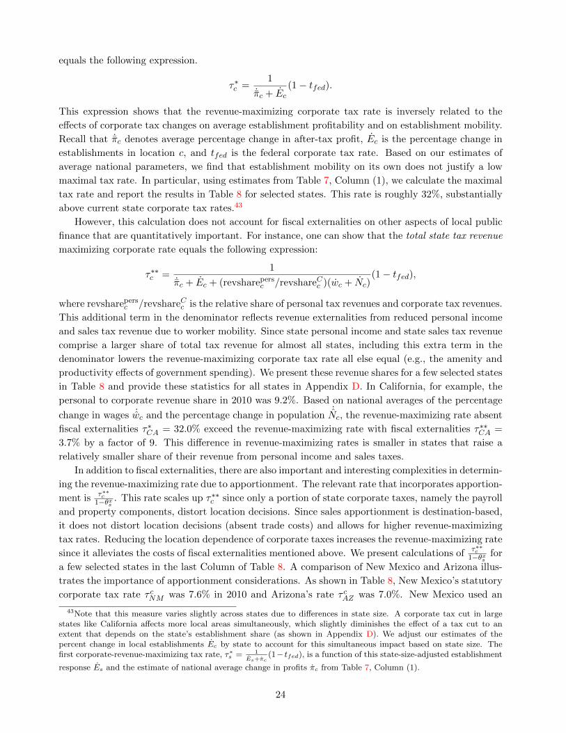
equals the following expression.

⌧⇤c =1

˙⇡c + Ec

(1� tfed).

This expression shows that the revenue-maximizing corporate tax rate is inversely related to the

e↵ects of corporate tax changes on average establishment profitability and on establishment mobility.

Recall that ˙⇡c denotes average percentage change in after-tax profit, Ec is the percentage change in

establishments in location c, and tfed is the federal corporate tax rate. Based on our estimates of

average national parameters, we find that establishment mobility on its own does not justify a low

maximal tax rate. In particular, using estimates from Table 7, Column (1), we calculate the maximal

tax rate and report the results in Table 8 for selected states. This rate is roughly 32%, substantially

above current state corporate tax rates.43

However, this calculation does not account for fiscal externalities on other aspects of local public

finance that are quantitatively important. For instance, one can show that the total state tax revenue

maximizing corporate rate equals the following expression:

⌧⇤⇤c =1

˙⇡c + Ec + (revsharepersc /revshareCc )(wc + Nc)(1� tfed),

where revsharepersc /revshareCc is the relative share of personal tax revenues and corporate tax revenues.

This additional term in the denominator reflects revenue externalities from reduced personal income

and sales tax revenue due to worker mobility. Since state personal income and state sales tax revenue

comprise a larger share of total tax revenue for almost all states, including this extra term in the

denominator lowers the revenue-maximizing corporate tax rate all else equal (e.g., the amenity and

productivity e↵ects of government spending). We present these revenue shares for a few selected states

in Table 8 and provide these statistics for all states in Appendix D. In California, for example, the

personal to corporate revenue share in 2010 was 9.2%. Based on national averages of the percentage

change in wages ˙wc and the percentage change in population ˙Nc, the revenue-maximizing rate absent

fiscal externalities ⌧⇤CA = 32.0% exceed the revenue-maximizing rate with fiscal externalities ⌧⇤⇤CA =

3.7% by a factor of 9. This di↵erence in revenue-maximizing rates is smaller in states that raise a

relatively smaller share of their revenue from personal income and sales taxes.

In addition to fiscal externalities, there are also important and interesting complexities in determin-

ing the revenue-maximizing rate due to apportionment. The relevant rate that incorporates apportion-

ment is ⌧⇤⇤c1�✓xs

. This rate scales up ⌧⇤⇤c since only a portion of state corporate taxes, namely the payroll

and property components, distort location decisions. Since sales apportionment is destination-based,

it does not distort location decisions (absent trade costs) and allows for higher revenue-maximizing

tax rates. Reducing the location dependence of corporate taxes increases the revenue-maximizing rate

since it alleviates the costs of fiscal externalities mentioned above. We present calculations of ⌧⇤⇤c1�✓xs

for

a few selected states in the last Column of Table 8. A comparison of New Mexico and Arizona illus-

trates the importance of apportionment considerations. As shown in Table 8, New Mexico’s statutory

corporate tax rate ⌧ cNM was 7.6% in 2010 and Arizona’s rate ⌧ cAZ was 7.0%. New Mexico used an

43Note that this measure varies slightly across states due to di↵erences in state size. A corporate tax cut in largestates like California a↵ects more local areas simultaneously, which slightly diminishes the e↵ect of a tax cut to anextent that depends on the state’s establishment share (as shown in Appendix D). We adjust our estimates of thepercent change in local establishments Ec by state to account for this simultaneous impact based on state size. Thefirst corporate-revenue-maximizing tax rate, ⌧⇤

s = 1

Es+⇡c(1� tfed), is a function of this state-size-adjusted establishment

response Es and the estimate of national average change in profits ⇡c from Table 7, Column (1).

24

equal-weighted apportionment formula with ✓wNM = ✓⇢NM = ✓xNM = 33% in 2010. Arizona, however,

put much more weight on sales as ✓xAZ = 80%. As a result, New Mexico’s revenue-maximizing rate

was roughly four times smaller than that of Arizona despite only a 0.6 percentage point di↵erence in

their statutory corporate rates. In particular,⌧⇤⇤NM

1�✓xNM= 2.1% and

⌧⇤⇤AZ1�✓xAZ

= 8.3%. Perhaps for this

reason, we have seen more states shift more weight towards the sales factor ✓xs as shown in Figure 3.

Overall, other tax factors, including apportionment formulae and di↵erences in the reliance on other

sources of tax revenue, account for the large geographic variation in the total revenue-maximizing

state corporate tax rates that range from 0.7% to 36.1%.

8 Conclusion

This paper evaluates the welfare e↵ects of cutting corporate income taxes on business owners, workers,

and landowners. This question is important for three reasons. First, the conventional view among

many economists and policy makers – that workers fully bear the incidence of corporate taxes in

an open economy – is based on fairly abstract arguments and less than fully convincing evidence.

Second, evaluating the welfare e↵ect of corporate taxes also highlights e�ciency consequences of

corporate taxation and has direct implications for revenue-maximizing rates. Third, the welfare

impacts of corporate tax cuts closely relate to the welfare impacts of a broad class of local economic

development policies that aim to entice businesses to locate in their jurisdictions.

We estimate the incidence of corporate taxes in four steps. First, we develop a local labor markets

framework with heterogeneously productive and monopolistically competitive firms. This framework

not only enables us to characterize the incidence on workers, firms, and landowners in terms of a

few parameters, but it can also be used to answer other important questions, such as the welfare

impacts of business location subsidies for individual companies, optimal local tax policy, and the inci-

dence of technological change. Second, we use state corporate tax apportionment rules and matched

establishment-firm data to construct a new measure of the e↵ective tax rate that businesses pay at

the local level. Third, we relate changes in these e↵ective rates to local outcomes and show that a 1%

cut in business taxes increases establishment growth by 3 to 4% over a ten-year period. Fourth, and

most importantly, we combine these three components – a new framework, a new measure of business

taxes, and new reduced form e↵ects of business taxes – to estimate the incidence of corporate taxes

on firm owners, workers, and landowners.

Three types of evidence support the validity of our incidence estimates. First, we show that our

reduced-form incidence estimates are robust to controlling for trends economic conditions, local labor

demand shocks, government spending changes, and a wide variety of other tax policy changes. Second,

estimates using external business tax changes from other states imply similar incidence estimates.

Third, the structural elasticities that rationalize our estimates are similar to those in the literature.

We unambiguously reject the view that workers bear 100% of the incidence of state corporate

tax cuts and find that firm owners bear a substantial portion of the incidence. The intuition for this

result is that non-tax considerations, namely heterogeneous productivity, can limit the mobility of

businesses. If a business is especially productive in a given location, small changes in taxes won’t have

large enough impacts on profitability to make changing locations attractive. For instance, technology

firms may still find it optimal to locate in Silicon Valley, even if corporate tax rates were increased

modestly. Consequently, firm owners bear a substantial portion of the incidence of corporate tax

changes, a result that starkly contrasts with the conventional wisdom.

25

References

Albouy, David. 2008. “Are Big Cities Bad Places to Live? Estimating Quality of Life acrossMetropolitan Areas.” National Bureau of Economic Research Working Paper 14472.

Albouy, David, and Bryan Stuart. 2013. “Urban Population and Amenities.” University of Michi-gan Working Paper.

Albouy, David, and Gabriel Ehrlich. 2012. “Metropolitan Land Values and Housing Productiv-ity.” National Bureau of Economic Research Working Paper 18110.

Arkolakis, Costas, Natalia Ramondo, Andres Rodrıguez-Clare, and Stephen Yeaple.2013. “Innovation and Production in the Global Economy.” National Bureau of Economic ResearchWorking Paper 18972.

Arulampalam, Wiji, Michael P. Devereux, and Giorgia Ma�ni. 2012. “The direct incidenceof corporate income tax on wages.” European Economic Review, 56(6): 1038 – 1054.

Auerbach, Alan J. 2002. “Taxation and Corporate Financial Policy.” In Handbook of Public Eco-nomics. Vol. 3. 1 ed., , ed. Alan J. Auerbach and Martin Feldstein, Chapter 19. Elsevier.

Auerbach, Alan J. 2006. “Who Bears the Corporate Tax? A Review of What We Know.” In TaxPolicy and the Economy. Vol. 20, , ed. James Poterba, 1–40. The MIT Press.

Autor, David H., David Dorn, and Gordon H. Hanson. 2013. “The China Syndrome: LocalLabor Market E↵ects of Import Competition in the United States.” American Economic Review,103(6): 2121–68.

Bartik, Timothy J. 1985. “Business Location Decisions in the United States: Estimates of the Ef-fects of Unionization, Taxes, and Other Characteristics of States.” Journal of Business & EconomicStatistics, 3(1): 14–22.

Bartik, Timothy J. 1991. Who Benefits from State and Local Economic Development Policies?W.E. Upjohn Institute for Employment Research.

Basker, Emek. 2005. “Selling a Cheaper Mousetrap: Wal-Mart’s E↵ect on Retail Prices.” Journalof Urban Economics, 58(2): 203–29.

Basu, Susanto. 1995. “Intermediate Goods and Business Cycles: Implications for Productivity andWelfare.” The American Economic Review, 85(3): pp. 512–531.

Beraja, Martin, Erik Hurst, and Juan Ospina. 2016. “The Aggregate Implications of RegionalBusiness Cycles.” National Bureau of Economic Research Working Paper 21956.

Bernthal, Jamie, Dana Gavrila, Katie Schumacher, Shane Spencer, and Katherine Sydor.2012. “Single Sales-Factor Corporate Income Tax Apportionment: Evaluating the Impact in Wis-consin.” The Wisconsin Department of Revenue.

Bradford, David F. 1978. “Factor Prices May Be Constant But Factor Returns Are Not.” EconomicsLetters, 1(3): 199–203.

Busso, Matias, Jesse Gregory, and Patrick Kline. 2013. “Assessing the Incidence and E�ciencyof a Prominent Place Based Policy.” American Economic Review, 103(2): 897–947.

Card, David. 2011. “The Return of the Firm to Labor Economics.” U.C. Berkeley.

Carlton, Dennis W. 1983. “The Location and Employment Choices of New Firms.” The Review ofEconomics and Statistics, 75(3).

CCH. 1980-2010. State Tax Handbook 1980-2010. CCH Incorporated State Tax Handbook, ToolkitMedia Group.

Chamberlain, Gary. 1984. “Chapter 22 Panel data.” In . Vol. 2 of Handbook of Econometrics, 1247– 1318. Elsevier.

26

Chirinko, Robert S., and Daniel J. Wilson. 2008. “State Investment Tax Incentives: A Zero-SumGame?” Journal of Public Economics, 92(12).

Clausing, Kimberly. 2013. “Who Pays The Corporate Tax In A Global Economy?” National TaxJournal, 66(1): 151–84.

Coibion, Olivier, Yuriy Gorodnichenko, and Johannes Wieland. 2012. “The Optimal Infla-tion Rate in New Keynesian Models: Should Central Banks Raise Their Inflation Targets in Lightof the Zero Lower Bound?” The Review of Economic Studies, 79(4): 1371–1406.

Cronin, Julie Anne, Emily Y. Lin, Laura Power, and Michael Cooper. 2013. “Distribut-ing The Corporate Income Tax: Revised U.S. Treasury Methodology.” National Tax Journal,66(1): 239–62.

CSG. 1976-2011. Book of the States. Council of State Governments.

Cullen, Zoe, and Juan Carlos Suarez Serrato. 2014. “State Corporate Taxes, Firm Mobility, andInnovation Productivity: Evidence from US patent data.” Stanford University and Duke UniversityWorking Paper.

Desai, Mihir A., C. Fritz Foley, and James R. Hines Jr. 2007. “Labor and Capital Sharesof the Corporate Tax Burden: International Evidence.” Who Pays the Corporate Tax in an OpenEconomy?

Devereux, Michael P., and Rachel Gri�th. 1998. “Taxes and the location of production: evi-dence from a panel of US multinationals.” Journal of Public Economics, 68(3): 335 – 367.

Devereux, Michael P, and Simon Loretz. 2007. “The E↵ects of EU Formula Apportionment onCorporate Tax Revenues.” Oxford University Centre for Business Taxation working paper.

Diamond, Rebecca. 2012. “The Determinants and Welfare Implications of US Workers’ DivergingLocation Choices by Skill: 1980-2000.” Harvard University Job Market Paper.

Duranton, Gilles, Laurent Gobillon, and Henry G. Overman. 2011. “Assessing the E↵ects ofLocal Taxation using Microgeographic Data.” The Economic Journal, 121(555): 1017–1046.

Fajgelbaum, Pablo D., Eduardo Morales, Juan Carlos Suarez Serrato, and Owen M.Zidar. 2015. “State Taxes and Spatial Misallocation.” National Bureau of Economic ResearchWorking Paper 21760.

Feldstein, Martin, and Marian Vaillant. 1998. “Can State Taxes Redistribute Income?” Journalof Public Economics, 68(3): 369–396.

Fuest, Clemens, Andreas Peichl, and Sebastian Siegloch. 2013. “Do Higher Corporate TaxesReduce Wages? Micro Evidence from Germany.” Institute for the Study of Labor Discussion Paper.

Fullerton, Don, and Gilbert E. Metcalf. 2002. “Tax Incidence.” In Handbook of Public Eco-nomics. Vol. 4, , ed. Alan J. Auerbach and Martin Feldstein, Chapter 26. Elsevier.

Gentry, William M., and R. Glenn Hubbard. 2000. “Tax Policy and Entrepreneurial Entry.”American Economic Review, 90(2): 283–287.

Glaeser, Edward L. 2008. Cities, Agglomeration, and Spatial Equilibrium. Oxford University Press.

Glaeser, Edward L. 2012. “Urban Public Finance.” National Bureau of Economic Research WorkingPaper 18244.

Glaeser, Edward L., and Joseph Gyourko. 2005. “Urban Decline and Durable Housing.” Journalof Political Economy, 113(2): pp. 345–000.

Goolsbee, Austan, and Edward L. Maydew. 2000. “Coveting thy neighbor’s manufacturing:the dilemma of state income apportionment.” Journal of Public Economics, 75(1): 125 – 143.

Gordon, Roger H., and James R. Hines. 2002. “International taxation.” In Handbook of PublicEconomics. Vol. 4, , ed. Alan J. Auerbach and Martin Feldstein, 1935 – 1995. Elsevier.

27

Gordon, Roger H., and John Douglas Wilson. 1986. “An Examination of MultijurisdictionalCorporate Income Taxation under Formula Apportionment.” Econometrica, 54(6): 1357–73.

Gravelle, Jane, and Kent Smetters. 2006. “Does the Open Economy Assumption Really MeanThat Labor Bears the Burden of a Capital Income Tax?” The B.E. Journal of Economic Analysis& Policy, 6(1): 1–44.

Gravelle, Jennifer. 2011. “Corporate Tax Incidence: Corporate Tax Incidence: A Review of Em-pirical Estimates and Analysis.” Congressional Budget O�ce.

Gravelle, Jennifer C. 2010. “Corporate Tax Incidence: Review of General Equilibrium Estimatesand Analysis.” Congressional Budget O�ce Working Paper 2010-03.

Greenstone, Michael, and Enrico Moretti. 2004. “Bidding for Industrial Plants: Does Winninga ‘Million Dollar Plant’ Increase Welfare?” MIT Department of Economics Working Paper 04-39.

Gyourko, Joseph, and Joseph Tracy. 1989. “The Importance of Local Fiscal Conditions inAnalyzing Local Labor Markets.” Journal of Political Economy, 97(5): 1208–31.

Hall, Robert E., and Charles I. Jones. 1999. “Why do Some Countries Produce So Much MoreOutput Per Worker than Others?” The Quarterly Journal of Economics, 114(1): 83–116.

Hamermesh, Daniel. 1993. Labor Demand. Princeton University Press.

Harberger, Arnold C. 1962. “The Incidence of the Corporation Income Tax.” Journal of PoliticalEconomy, 70(3): pp. 215–240.

Hassett, Kevin A., and Aparna Mathur. 2015. “A spatial model of corporate tax incidence.”Applied Economics, 47(13): 1350–1365.

Haughwout, Andrew F., and Robert P. Inman. 2001. “Fiscal policies in open cities with firmsand households.” Regional Science and Urban Economics, 31(2-3): 147 – 180.

Head, K., and T. Mayer. 2013. “Gravity Equations: Workhorse,Toolkit, and Cookbook.” Handbookof International Economics Vol. 4.

Heider, Florian, and Alexander Ljungqvist. 2014. “As Certain as Debt and Taxes: Estimat-ing the Tax Sensitivity of Leverage from Exogenous State Tax Changes.” Journal of FinancialEconomics.

Helms, L. Jay. 1985. “The E↵ect of State and Local Taxes on Economic Growth: A Time Series–Cross Section Approach.” The Review of Economics and Statistics, 67(4): pp. 574–582.

Hendren, Nathaniel. 2015. “The Policy Elasticity.” Tax Policy and the Economy, Volume 30.University of Chicago Press.

Hines, James. 2009. “Income Misattribution under Formula Apportionment.” NBER working paper15185.

Hines, James R. 1997. “Altered States: Taxes and the Location of Foreign Direct Investment inAmerica.” National Bureau of Economic Research Working Paper 4397.

Holmes, Thomas J. 1998. “The E↵ect of State Policies on the Location of Manufacturing: Evidencefrom State Borders.” Journal of Political Economy, 106(4): pp. 667–705.

Hopenhayn, Hugo A. 1992. “Entry, Exit, and Firm Dynamics in Long Run Equilibrium.” Econo-metrica, 60(5): pp. 1127–1150.

Kline, Patrick. 2010. “Place Based Policies, Heterogeneity, and Agglomeration.” American Eco-nomic Review, 100(2): 383–87.

Kline, Patrick, and Enrico Moretti. 2013. “People, Places, and Public Policy: Some SimpleWelfare Economics of Local Economic Development Programs.” U.C. Berkeley Working Paper.

28

Kline, Patrick, and Enrico Moretti. 2014. “Local Economic Development, AgglomerationEconomies and the Big Push: 100 Years of Evidence from the Tennessee Valley Authority.” Quar-terly Journal of Economics.

Kotliko↵, Laurence J., and Lawrence H. Summers. 1987. “Tax Incidence.” In Handbook ofPublic Economics. Vol. 2, , ed. Alan J. Auerbach and Martin Feldstein, Chapter 16. Elsevier.

Krugman, Paul R. 1979. “Increasing returns, monopolistic competition, and international trade.”Journal of International Economics, 9(4): 469 – 479.

Levchenko, Andrei A., and Jing Zhang. 2012. “Ricardian Productivity Di↵erences and the Gainsfrom Trade.” Research Seminar in International Economics, University of Michigan Working Papers633.

Liu, Li, and Rosanne Altshuler. 2013. “Measuring the Burden of the Corporate Income TaxUnder Imperfect Competition.” National Tax Journal, 66(1): 215–238.

McFadden, Daniel. 1978. “Modeling the Choice of Residential Location.” In Spatial InteractionTheory and Planning Models. , ed. Karlqvist, Lundqvist, Snickars and Weibull. Amsterdam: NorthHolland.

McLure Jr., Charles E. 1977. “State Corporate Income Tax: Lambs in Wolves’ Clothing?” O�ceof Tax Analysis Paper 25.

McLure Jr., Charles E. 1982. “The Elusive Incidence of the Corporate Income Tax: The StateCase.” National Bureau of Economic Research Working Paper 616.

Melitz, Marc J. 2003. “The Impact of Trade on Intra-Industry Reallocations and Aggregate IndustryProductivity.” Econometrica, 71(6): pp. 1695–1725.

Mian, Atif, and Amir Sufi. 2016. “What Explains the 2007-2009 Drop in Employment?” Econo-metrica.

Moretti, Enrico. 2010. “Local Multipliers.” American Economic Review, 100(2): 373–77.

Moretti, Enrico. 2011. “Local Labor Markets.” In Handbook of Labor Economics. Vol. 4, , ed. O.Ashenfelter and D. Card, Chapter 14, 1237–1313. Elsevier.

Moretti, Enrico. 2013. “Real Wage Inequality.” American Economic Journal: Applied Economics,5(1): 65–103.

Newman, Robert J. 1983. “Industry Migration and Growth in the South.” The Review of Eco-nomics and Statistics, 65(1): pp. 76–86.

Notowidigdo, Matthew J. 2013. “The Incidence of Local Labor Demand Shocks.” University ofChicago Booth School of Business.

Papke, Leslie E. 1987. “Subnational Taxation and Capital Mobility: Estimates of Tax-Price Elas-ticities.” National Tax Journal, 40(2).

Papke, Leslie E. 1991. “Interstate Business Tax Di↵erentials and New Firm Location: Evidencefrom Panel Data.” Journal of Public Economics, 45(1): 47 – 68.

Rathelot, Roland, and Patrick Sillard. 2008. “The Importance of Local Corporate Taxes inBusiness Location Decisions: Evidence from French Micro Data.” The Economic Journal, 118.

Roback, Jennifer. 1982. “Wages, Rents, and the Quality of Life.” Journal of Political Economy,90(6): 1257–78.

Rosen, Sherwin. 1979. “Wage-Based Indexes of Urban Quality of Life.” In Current Issues in UrbanEconomics. , ed. Mahlon R. Straszheim Peter M. Mieszkowski. Johns Hopkins University Press.

Rothenberg, Alexander D. 2012. “Transport Infrastructure and Firm Location Choice in Equi-librium: Evidence from Indonesia’s Highways.” The RAND Corporation Working Paper.

29

Ruggles, Steven, et al. 2010. “Integrated Public Use Microdata Series: Version 5.0.” Minneapolis:University of Minnesota [Machine-readable database].

Saez, Emmanuel, and Stefanie Stantcheva. 2013. “Generalized Social Marginal Welfare Weightsfor Optimal Tax Theory.” National Bureau of Economic Research Working Paper 18835.

Scheuer, Florian. 2014. “Entrepreneurial Taxation with Endogenous Entry.” American EconomicJournal: Economic Policy, 6(2): 126–63.

Seegert, Nathan. 2012. “Optimal Taxation with Volatility: A Theoretical and Empirical Decom-position.” University of Michigan Job Market Paper.

Siegloch, Sebastian. 2014. “Employment E↵ects of Local Business Taxes.” Annual Conference 2014(Hamburg): Evidence-based Economic Policy.

Suarez Serrato, Juan Carlos, and Philippe Wingender. 2011. “Estimating the Incidence ofGovernment Spending.” U.C. Berkeley and International Monetary Fund Working Paper.

Syverson, Chad. 2011. “What Determines Productivity?” Journal of Economic Literature,49(2): 326–65.

Tolley, George S. 1974. “The welfare economics of city bigness.” Journal of Urban Economics,1(3): 324 – 345.

Topel, Robert H. 1986. “Local Labor Markets.” Journal of Political Economy, 94(3): S111–43.

Train, Kenneth. 2009. Discrete Choice Methods with Simulation. . 2 ed., Cambridge UniversityPress.

Wilson, Daniel J. 2009. “Beggar Thy Neighbor? The In-State, Out-of-State, and Aggregate E↵ectsof R&D Tax Credits.” Review of Economics and Statistics, 91(2): 431–436.

Yagan, Danny. 2015. “Capital Tax Reform and the Real Economy: The E↵ects of the 2003 DividendTax Cut.” National Bureau of Economic Research Working Paper 21003.

Zidar, Owen M. 2014. “Tax Cuts for Whom? Heterogeneous E↵ects of Income Tax Changes onGrowth and Employment.” University of Chicago Booth School of Business.

30

Table 3: Summary Statistics

Variable Mean S.D. Min Max N

Annual Outcome Data from BEA and CBPYear 1995 8.9 1980 2010 15190Log Population: lnNc,t 13.8 1.1 10.9 16.1 15190Log Employment: lnLc,t 13.2 1.2 9.4 15.6 15190Log Establishments: lnEc,t 10.0 1.2 6.5 12.4 15190

Annual Data on Apportionment Rules and Corporate, Personal, and Business Tax RatesState Corporate Tax Apportionment ParametersPayroll Apportionment Weight: ✓ws,t 22.7 11.6 0.0 33.3 15190Property Apportionment Weight: ✓⇢s,t 22.8 11.6 0.0 33.3 15190Sales Apportionment Weight: ✓xs,t 54.5 23.2 25 100 15190

Corporate IncomeRate: ⌧ cs,t 6.6 3.0 0.0 12.3 15190% Change in Net-of-Rate: � ln (1� ⌧ c)s,t,t�1 -0.01 0.4 -5.4 3.8 15190

Personal IncomeE↵ective Rate: ⌧ is,t 2.6 1.7 0.0 7.4 15190% Change in Net-of-Rate: � ln (1� ⌧ i)s,t,t�1 0.03 0.2 -3.3 2.5 15190

Business IncomeRate: ⌧ bc,t 3.1 1.1 0.3 5.4 15190% Change in Net-of-Rate: � ln (1� ⌧ b)c,t,t�1 -0.01 0.2 -1.8 1.2 15190

Decadal DataYear 2000 8.2 1990 2010 1470% Change in Population: � lnNc,t,t�10 11.2 10.4 -16.6 76.1 1470% Change in Establishments: � lnEc,t,t�10 15.2 16.5 -23 126.2 1470% Change in Adjusted Wages: � lnwc,t,t�10 -2.8 7.2 -31.2 14.9 1470% Change in Adjusted Rents: � ln rc,t,t�10 8.5 12.0 -41.4 43.4 1470% Change in Net-of-Corp.-Rate: � ln (1� ⌧ c)s,t,t�10 -0.1 1.1 -5.4 4.5 1470% Change in Net-of-Pers.-Rate: � ln (1� ⌧ i)s,t,t�10 -1.3 1.1 -5.3 1.3 1470% Change in Net-of-Bus.-Rate: � ln (1� ⌧ b)c,t,t�10 -0.8 0.6 -2.8 1.3 1470% Change in Gov. Expend./Capita: � lnGc,t,t�10 0.0 0.6 -13.3 11.6 1470Bartik Shock: Bartikc,t,t�10 7.8 4.8 -15.2 26.0 1470

Sources: BEA, CBP, Zidar (2014), Suarez Serrato and Wingender (2011). Corporate tax sources in Section 4.

31

Table 4: E↵ects of Business Tax Cuts on Local Economic Activity over 10 Years

A. Establishment Growth (1) (2) (3) (4) (5) (6)

� ln Net-of-Business-Tax Rate 4.07** 3.35** 4.06** 4.14** 3.91** 3.24**(1.82) (1.43) (1.83) (1.80) (1.78) (1.41)

Bartik 0.59*** 0.57***(0.19) (0.18)

� ln Gov Expend/Capita -0.01 -0.01(0.01) (0.01)

� State ITC -0.46 -0.17(0.32) (0.30)

Change in Other States’ Taxes -4.66*** -4.18***(1.60) (1.43)

Observations 1,470 1,470 1,470 1,470 1,470 1,470R-squared 0.472 0.491 0.472 0.475 0.481 0.500

B: Other Outcomes Population Growth Wage Growth Rental Cost Growth(1) (2) (1) (2) (1) (2)

� ln Net-of-Business-Tax Rate 4.28** 3.74** 1.45 0.78 1.17 0.32(1.65) (1.48) (0.94) (0.82) (1.44) (1.37)

Bartik 0.44** 0.56*** 0.70**(0.19) (0.08) (0.27)

Observations 1,470 1,470 1,470 1,470 1,470 1,470R-squared 0.085 0.113 0.402 0.490 0.139 0.189

Notes: This table shows the e↵ects of local business tax changes over ten years on local establishment growth in panel

A and on population growth, wage growth, and rental cost growth in panel B. The data are decade changes from 1980-

1990, 1990-2000, and 2000-2010 for 490 county-groups. See Section 4 for data sources. In panel A, Col (2)-(6) show

that the e↵ect of business taxes is robust to controlling for Bartik shocks in Col (2), per capita government spending

changes in Col (3), state investment tax credit changes in Col (4), external tax shocks due to changes in tax rules of

other states in Col (5), and all of these controls in Col (6). �2 tests indicate that the coe�cients in Col (1) and Col

(2) are not statistically di↵erent. Similarly, the negative e↵ect from tax cuts in other states is not statistically di↵erent

than the positive e↵ect of tax cuts. Panel B provides the results for Col (1) and (2) for three other outcomes. �2 tests

also indicate that the coe�cients in Col (1) and Col (2) are not statistically di↵erent for each of the outcomes. The full

tables similar to panel A for the other three outcomes – population, wages, and rental cost – are provided in Appendix

Tables A6, A7, and A8. Non-parametric graphs showing mean outcome changes by business tax change bins are shown

for each outcome in Appendix Figures A10, A11, A12, and A13, respectively. All regressions use population as weights

and include year fixed e↵ects and dummies for states in the industrial midwest in the 1980s. Table A30 and A31 show

results with controls for tax rates and changes an tax rates, respectively, for each of the four reduced-form outcomes.

Standard errors clustered by state are in parentheses and *** p<0.01, ** p<0.05, * p<0.1.

32

Table 5: Estimates of Economic Incidence Using Reduced-Form E↵ects

A. Incidence B. Share of Incidence(1) (2) (3) (4) (5) (6) (1) (2) (3) (4) (5) (6)

Landowners 1.17 1.17 1.17 .32 1.86 .62 .30 .34 .27 .18 .42** .29*(1.43) (1.43) (1.43) (1.36) (1.56) (.60) (.19) (.24) (.2) (.48) (.17) (.16)

Workers 1.1* .69 1.1* .68 .98 .58* .28*** .20 .25*** .37 .22* .28***(.59) (.44) (.59) (.52) (.84) (.33) (.09) (.16) (.07) (.43) (.12) (.08)

Firmowners 1.63* 1.63* 2.08** .81 1.54* .9*** .42*** .47*** .48*** .45*** .35*** .43***(.90) (.90) (.95) (1.4) (.92) (.34) (.12) (.10) (.17) (.13) (.09) (.10)

Conventional View Test�2 of (SW = 100% & SF = 0%) 132.67 108.14 48.8 6.96 76.27 195.92P-value 0.00 0.00 0.00 0.01 0.00 0.00

SpecificationNet-of-Business Tax Y Y Y Y Y N Y Y Y Y Y NNet-of-Corporate Tax N N N N N Y N N N N N YHousing share ↵ .3 .65 .3 .3 .3 .3 .3 .65 .3 .3 .3 .3Output elasticity ratio �/� .9 .9 .5 .9 .9 .9 .9 .9 .5 .9 .9 .9Bartik Control N N N Y Y N N N N Y Y NNet-of-Personal Tax Control N N N N Y N N N N N Y N

Notes: This table shows the estimates of the economic incidence expressions from Table 1. The data are decade changes from 1980-1990, 1990-2000, and 2000-2010

for 490 county-groups. See Section 4 for data sources. Results were produced by implementing Equation 21 using the specification in Column (1) of Table 4 unless

otherwise specified. Columns (2) and (3) use the same specification as Column (1) but with di↵erent calibrated values of the expenditure share on housing ↵ and

the ratio of output elasticities �/�. Column (4) controls for Bartik shocks. Column (5) controls for Bartik shocks as well as growth in the net-of-personal tax rate,

i.e., � ln(1 � ⌧ ic). Column (6) uses the net-of-statutory-corporate tax keep rate, i.e., � ln(1 � ⌧ c

c ) rather than the business keep rate, i.e., � ln(1 � ⌧ bc ), which is

used in Columns (1)-(5). Appendix Table A19 includes many supplemental tax base controls and Appendix Table A20 includes results with additional controls for

state political, economic, and fiscal policy conditions. More results using statutory state corporate tax rates are in Appendix Table A21. The conventional view

test evaluates the joint hypothesis that the share of incidence for workers equals 100% and the share for firm owners equals 0%. Note that Columns (4) and (5) use

Bartik and net-of-personal taxes as controls but does not use the point estimates for incidence share inference beyond that purpose; Table 7 provides results that use

these estimates to discipline our estimates of structural elasticities and resulting incidence share estimates and conventional view tests. Regressions use population as

weights and include year fixed e↵ects and dummies for states in the industrial midwest in the 1980s. See Section 4.3 for details on calibration values. Standard errors

clustered by state are in parentheses and *** p<0.01, ** p<0.05, * p<0.1.

33

Table 6: Minimum Distance Estimates of Structural Parameters

A. All ShocksCalibrated Parameters (1) (2) (3) (4) (5) (6) (7)Output Elasticity � 0.150 0.150 0.150 0.200 0.250 0.150 0.250Housing Share ↵ 0.300 0.500 0.650 0.300 0.300 0.300 0.500Elasticity of Product -2.500 -2.500 -2.500 -2.500 -2.500 -4.000 -4.000Demand "PD

Estimated ParametersIdiosyncratic Location 0.277** 0.271** 0.233** 0.321* 0.304 0.149 0.136Productivity Disperion �F (0.138) (0.120) (0.092) (0.186) (0.186) (0.096) (0.093)

Idiosyncratic Location 0.829*** 0.686*** 0.621*** 0.845*** 0.843*** 0.839*** 0.649**Preference Dispersion �W (0.282) (0.260) (0.230) (0.294) (0.295) (0.294) (0.253)

Elasticity of Housing 0.513 2.185 1.157 1.600 0.707 1.995 2.812Supply ⌘ (1.417) (6.206) (2.661) (5.065) (2.301) (7.320) (13.688)

Overid Test (p-value) 0.458 0.390 0.393 0.385 0.444 0.390 0.507

B. Business Tax Shock C. All Shocks, Estimated "PD

Calibrated Parameters (1) (2) (3) (4) (5) (6) (7)Output Elasticity � 0.150 0.150 0.250 0.150 0.150 0.150 0.250Housing Share ↵ 0.300 0.650 0.300 0.300 0.300 0.650 0.300Elasticity of Product -2.500 -2.500 -2.500 -4.000 Estimated BelowDemand "PD

Estimated ParametersIdiosyncratic Location 0.119* 0.117* 0.106 0.048 0.109 0.105 0.138Productivity Dispersion �F (0.065) (0.064) (0.075) (0.039) (0.392) (0.194) (0.411)

Idiosyncratic Location 0.188 0.128 0.171 0.170 0.892*** 0.571** 0.753***Preference Dispersion �W (0.184) (0.147) (0.176) (0.175) (0.337) (0.234) (0.245)

Elasticity of Housing 6.367 5.724 7.328 6.424 1.925 1.783 3.056Supply ⌘ (15.899) (13.090) (20.574) (16.136) (8.085) (6.503) (25.617)

Elasticity of Product -4.704 -4.439 -4.986Demand "PD (11.945) (6.471) (12.190)

Overid Test (p-value) 0.117 0.117 0.098 0.088 0.251 0.334 0.290

Notes: This table shows the estimated parameters of our model. The data are decade changes from 1980-1990, 1990-

2000, and 2000-2010 for 490 county-groups. See Section 4 for data sources. Panel A presents estimates from models with

business tax, personal tax, and Bartik shocks relying on 12 moments to estimate 3 parameters for a variety of assumed

values of ↵, � and "PD. Panel B uses only the business tax shock relying on 4 moments to estimate 3 parameters

for a variety of assumed values of ↵, � and "PD. Panel C presents estimates from “all shocks” models to estimate

4 parameters, including "PD, for various calibrated values of � and ↵. See Section 6 for more details on estimation.

Regressions use initial population as weights and include year fixed e↵ects and dummies for states in the industrial

midwest in the 1980s. Standard errors clustered by state are in parentheses and *** p<0.01, ** p<0.05, * p<0.1.34

Table 7: Estimates of Economic Incidence Using Estimated Structural Parameters

Incidence Shares of Incidence(1) (2) (3) (4) (5) (1) (2) (3) (4) (5)

All Shocks Business All Shocks All Shocks Business All ShocksCalibrated Parameters Tax Estimated "PD Tax Estimated "PD

Output Elasticity � 0.150 0.150 0.150 0.150 0.150 0.150 0.150 0.150 0.150 0.150Housing Share ↵ 0.300 0.650 0.300 0.300 0.300 0.300 0.650 0.300 0.300 0.300Elasticity of Product -2.500 -2.500 -4.000 -2.500 -4.704 -2.500 -2.500 -4.000 -2.500 -4.704Demand "PD (11.945) (11.945)

Estimated IncidenceWages w 0.944** 1.088** 0.655* 0.839 0.646

(0.408) (0.457) (0.348) (0.847) (1.028)

Landowners r 1.111 0.886 0.428 0.591 0.420 0.410 0.376 0.207 0.261 0.202(1.119) (1.052) (1.079) (1.373) (1.517) (0.263) (0.339) (0.434) (0.430) (0.621)

Workers w � ↵r 0.611** 0.512 0.527* 0.662 0.520 0.225* 0.217 0.255 0.292** 0.250(0.293) (0.355) (0.269) (0.517) (0.703) (0.134) (0.197) (0.185) (0.142) (0.290)

Firm Owners ⇡ 0.990*** 0.958*** 1.110*** 1.014*** 1.141 0.365** 0.407** 0.537* 0.447 0.548(0.092) (0.103) (0.157) (0.191) (1.012) (0.168) (0.164) (0.297) (0.392) (0.734)

Test of Standard View (p-value) 0.000 0.000 0.000 0.000 0.026

Elasticity of Labor 0.780** 0.757 0.958 4.188 0.902Supply "LS (0.386) (0.729) (0.588) (4.795) (0.645)

Elasticity of Labor -1.766*** -1.867*** -2.457*** -2.485*** -2.933Demand "LD (0.269) (0.252) (0.646) (0.692) (6.731)

Notes: This table shows structural estimates of economic incidence from our model. The Incidence panel shows the estimates of tax changes from our three minimum

distance specifications: using all shocks, only business taxes, and all shocks with estimated "PD, respectively. See Table 6 for details about the estimation of the related

structural models. The Shares of Incidence panel presents the shares of total economic gains to each agent that correspond to each specification. The conventional

view test evaluates the joint hypothesis that the share of incidence for workers equals 100% and the share for firm owners equals 0%. Panel (b) presents the associated

structural elasticities. Standard errors clustered by state are in parentheses and *** p<0.01, ** p<0.05, * p<0.1.

35

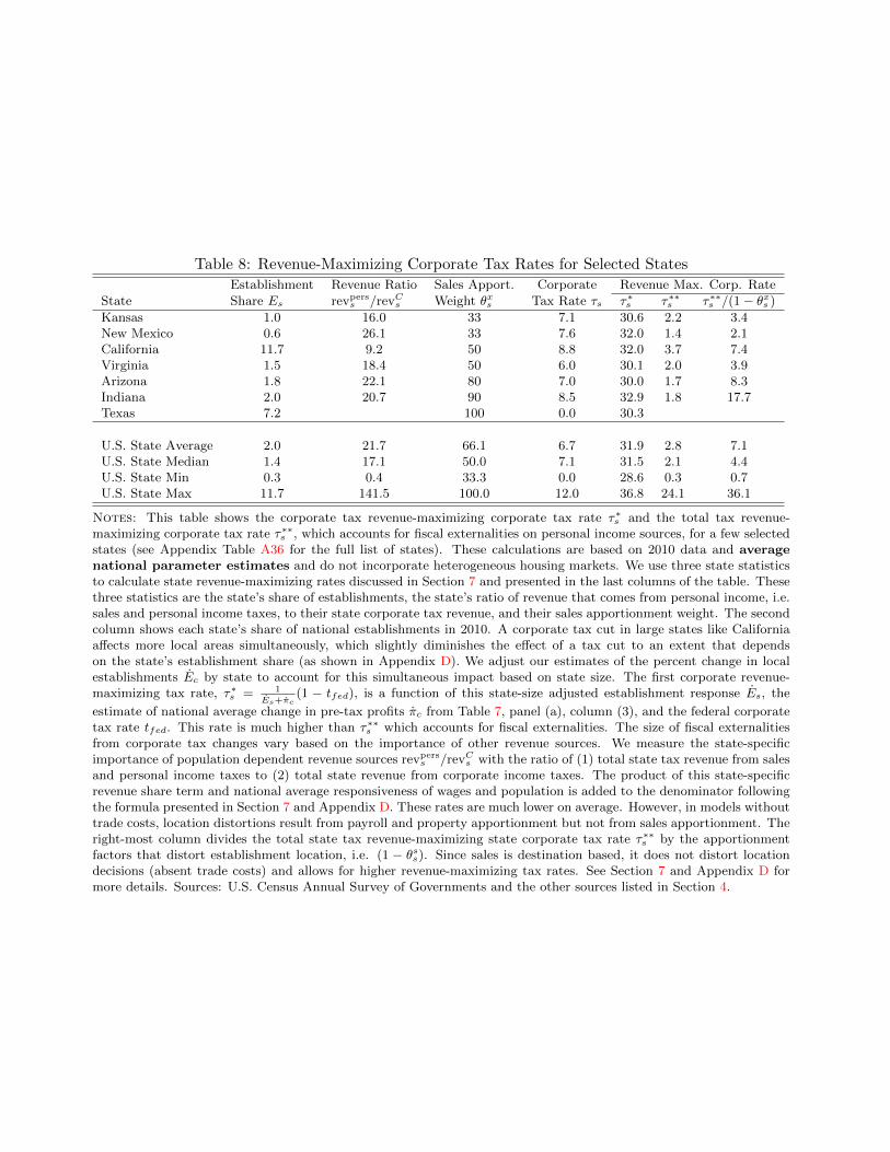
Table 8: Revenue-Maximizing Corporate Tax Rates for Selected StatesEstablishment Revenue Ratio Sales Apport. Corporate Revenue Max. Corp. Rate

State Share Es revperss /revC

s Weight ✓xs Tax Rate ⌧s ⌧⇤s ⌧⇤⇤

s ⌧⇤⇤s /(1� ✓xs )

Kansas 1.0 16.0 33 7.1 30.6 2.2 3.4New Mexico 0.6 26.1 33 7.6 32.0 1.4 2.1California 11.7 9.2 50 8.8 32.0 3.7 7.4Virginia 1.5 18.4 50 6.0 30.1 2.0 3.9Arizona 1.8 22.1 80 7.0 30.0 1.7 8.3Indiana 2.0 20.7 90 8.5 32.9 1.8 17.7Texas 7.2 100 0.0 30.3

U.S. State Average 2.0 21.7 66.1 6.7 31.9 2.8 7.1U.S. State Median 1.4 17.1 50.0 7.1 31.5 2.1 4.4U.S. State Min 0.3 0.4 33.3 0.0 28.6 0.3 0.7U.S. State Max 11.7 141.5 100.0 12.0 36.8 24.1 36.1

Notes: This table shows the corporate tax revenue-maximizing corporate tax rate ⌧⇤s and the total tax revenue-

maximizing corporate tax rate ⌧⇤⇤s , which accounts for fiscal externalities on personal income sources, for a few selected

states (see Appendix Table A36 for the full list of states). These calculations are based on 2010 data and average

national parameter estimates and do not incorporate heterogeneous housing markets. We use three state statisticsto calculate state revenue-maximizing rates discussed in Section 7 and presented in the last columns of the table. Thesethree statistics are the state’s share of establishments, the state’s ratio of revenue that comes from personal income, i.e.sales and personal income taxes, to their state corporate tax revenue, and their sales apportionment weight. The secondcolumn shows each state’s share of national establishments in 2010. A corporate tax cut in large states like Californiaa↵ects more local areas simultaneously, which slightly diminishes the e↵ect of a tax cut to an extent that dependson the state’s establishment share (as shown in Appendix D). We adjust our estimates of the percent change in localestablishments Ec by state to account for this simultaneous impact based on state size. The first corporate revenue-maximizing tax rate, ⌧⇤

s = 1

Es+⇡c(1 � tfed), is a function of this state-size adjusted establishment response Es, the

estimate of national average change in pre-tax profits ⇡c from Table 7, panel (a), column (3), and the federal corporatetax rate tfed. This rate is much higher than ⌧⇤⇤

s which accounts for fiscal externalities. The size of fiscal externalitiesfrom corporate tax changes vary based on the importance of other revenue sources. We measure the state-specificimportance of population dependent revenue sources revpers

s /revCs with the ratio of (1) total state tax revenue from sales

and personal income taxes to (2) total state revenue from corporate income taxes. The product of this state-specificrevenue share term and national average responsiveness of wages and population is added to the denominator followingthe formula presented in Section 7 and Appendix D. These rates are much lower on average. However, in models withouttrade costs, location distortions result from payroll and property apportionment but not from sales apportionment. Theright-most column divides the total state tax revenue-maximizing state corporate tax rate ⌧⇤⇤

s by the apportionmentfactors that distort establishment location, i.e. (1 � ✓ss). Since sales is destination based, it does not distort locationdecisions (absent trade costs) and allows for higher revenue-maximizing tax rates. See Section 7 and Appendix D formore details. Sources: U.S. Census Annual Survey of Governments and the other sources listed in Section 4.

Figure 1: The Impact of a Corporate Tax Cut on Workers and Firm Owners

I. E↵ects on Each Local EstablishmentA. Before Tax Cut B. A Corporate Tax Cut Has 3 E↵ects

DMR

$

y

p0

MC0

∝w

DMR

$

y

p0

MC0M !C .

1

23

II. Equilibrium E↵ects on Local Wages and After-Tax ProfitsC. Wage Increase w Determined in Labor Market D. Net E↵ect on After-Tax Profits

L0

w0

S0

D0 !D

L

w

!w

!L

w =

ΔDΔ(1−τ )#

$%

&

'(

ε LS −ε LD. !p

∝w

DMR

$

y

p0

MC0M !C .

. .

Notes: A. Monopolistically competitive establishments earn profits, which are divided into taxes and after-taxprofits. B. Cutting corporate taxes has three e↵ects on local establishments: a corporate tax cut reduces theestablishment’s (1) tax liability and (2) capital wedge mechanically. (3) Establishments enter the local area andbid up wages by w percent. C. Wage increases are determined in the local labor market as workers move in,house prices increase, each establishment hires fewer workers, and some marginal establishments leave. D. Thecumulative percentage increase on profits ⇡ depends on the magnitude of wage increases. We derive the change inlocal labor demand, "LS , and "LD from microfoundations and express them in terms of a few estimable parametersin Section 1. Empirical estimates of these parameters, which govern the three e↵ects above are provided in Tables 6and A33 and discussed in Section 6. Note that these e↵ects are enumerated to help provide intuition, but the formalmodel does not include dynamics. The model shows how the spatial equilibrium changes when states cut corporate taxes.

37

Figure 2: State Corporate Tax Rates

A. Number of Corporate Tax Changes by State since 1979

B. Corporate Tax Rates by State in 2012

Notes: These figures show statistics on state statutory corporate tax rates across states. See Appendix Figures A2,

A3, A4, and A5 for similar figures on state corporate tax apportionment rates, 30 year changes in corporate rates and

apportionment rules, state establishment and population shares, and 30 year changes in establishment and population

shares, respectively.

38

Figure 3: Histogram of Sales Apportionment Weights by Decade

010

20

30

40

010

20

30

40

20 40 60 80 100 20 40 60 80 100

1980 1990

2000 2010

Num

ber

of S

tate

s

Sales Apportionment Weight

Notes: This figure shows a histogram of the weight on sales activity that states use to apportion the national profits

of multi-state firms for tax purposes. Many states have increased their sales apportionment weights in recent decades.

Forty states used a one-third weight in 1980. As of 2010, more states put half or full 100% weight on sales activity than

the number that still uses the traditional one-third weight. See Section 4.2.1 for a description of state corporate tax

apportionment rules.

39

Figure 4: Cumulative E↵ects of Business Tax Cuts on Establishment Growth

A. Cumulative Annual E↵ects without leads

01

23

45

Percent

0 2 4 6 8 10Year

B. Cumulative Annual E↵ects with leads

F-test all leads are 0 has p-value= 0.92 F-test all lags are 0 has p-value= 0.036

-10

-50

510

Perc

ent

-10 -5 0 5 10Year

Cumulative Effect no leads Cumulative Effect w/ leadsLong Difference Point Estimate 95 % Confidence Interval

Notes: This figure shows the cumulative annual e↵ects of local business tax cuts on local establishment growth over

di↵erent time horizons. Panel A plots the sum of the point estimates in Col (4) of Table A5 and 90% confidence interval

for each time horizon. Panel B plots the sum of the point estimates in Col (7) of Table A5 and 90% confidence interval

for each time horizon starting with the greatest lead. In addition, it reports the p-values for the F-test that all leads

and lags are jointly equal to zero, which is also reported in Col 7 of Table A5. The square shows the point estimate

and 95% confidence interval for the long-run e↵ect of a one percent businesses tax cut on establishment growth, which

corresponds to the estimate reported in Col (4) of Table 4. See Section 4 for data sources and Section 5 for estimation

details.40

Figure 5: Robustness of Economic Incidence

Panel (a)Firm Owner’s Share of Incidence for ↵ = 0.3 and Calibrated Values of � and "PD

* Baseline-5

-4-3

-2El

astic

ity o

f Pro

duct

Dem

and:

εPD

0 .1 .2 .3 .4 .5Output Elasticity of Labor: γ

.3

.4

.5

.6

.7

.8

.9

Shar

e to

Firm

Own

ers

Panel (b)Firm Owner’s Share of Incidence for � = .15 and Calibrated Values of ↵ and "PD

* Baseline

-5-4

-3-2

Elas

ticity

of P

rodu

ct D

eman

d: εP

D

0 .2 .4 .6 .8 1Housing Expenditure Share: α

.2

.3

.4

.5

.6

.7

Shar

e to

Firm

Own

ers

Notes: This figure shows that our baseline empirical result – that firm owners bear a substantial share of incidence – is

robust to using a wide range of calibrated parameter values. The figures plot firm owner incidence shares for a variety

of parameter values and illustrates that our baseline parameters values of � = 0.15, "PD = �2.5, and ↵ = .3 give a

conservative share of the incidence to firm owners. Using calibrations with more elastic product demand elasticities,

while holding constant � = 0.15 in Panel A (or while holding constant ↵ = .3 in Panel B), does not change the result that

the share to firm owners ranges between 35 and 40%. Increasing the calibrated � in Panel A (or ↵ in Panel B) generally

increases the share accruing to firm owners. Overall, larger product demand elasticities "PD, housing expenditure shares

↵, and/or larger output elasticities of labor � result in larger burdens on firm owners. See Section 6 for more detail.41

Appendices for Online Publication

This appendix contains several sections. Section A discusses tax measurement, supplemental datasources, and the variation in tax rates. Section B provides a characterization of the establishmentproblem under apportionment and several derivations of expressions in the main text. Section Cdiscusses the e↵ects of a local corporate tax change on the welfare of agents in other locations andon e�ciency. Section D derives revenue-maximizing corporate tax rate expressions in the main text.Section E contains a detailed description of estimates underlying Figure 4 in the main section, adiscussion of several supplemental robustness tables for key tables in the main text, a step-by-stepguide through our estimation approach, an alternative equation-by-equation discussion of estimationthat provides more intuition for the estimating equations relative to the system approach in the maintext, and details on the structural estimation with all shocks. Section F and G provide more detailon our robustness exercises that account for the welfare e↵ects of changes in government spendingand local prices, respectively.

A Data

This section describes advantages of local areas called PUMAs in Section A.1, the derivation ofcomposition-adjusted outcomes in Section A.2 and the tax data used in Section A.3. In particular,we provide institutional detail on apportionment and how that informed how we constructed taxrates that account for apportionment in Section A.3.1, the sources for corporate tax parameters inthe main text in Section A.3.2, the source and methodological overview for our personal income taxrate data in Section A.3.3, a discussion of the limitations of our tax change measure in Section A.3.4,data on local prices in Section A.4, and data sources for variables that only appear in appendix tablesin Section A.5. Finally, section A.6 describes variation in tax rates.

A.1 Advantages of Using PUMAs

There are several advantages of using “consistent public-use micro-data areas (PUMAs).” First, thisgeographical definition depends on county boundaries that are geographically consistent since 1980.This fact allows us to generate data series at a yearly frequency using data for individual counties.Moreover, it allows us to use micro-data from the U.S. census to create wage, rental cost, and homevalue indexes for geographically consistent areas across censuses. Second, the level of aggregation doesnot straddle state lines, in contrast to other definitions of local economies. This feature is beneficialsince some of the policies we analyze, namely changes in statutory corporate tax rates, vary at thestate level. Since local areas vary in industrial composition, apportionment rules create within statevariation in the taxes businesses pay. To our knowledge, this paper is the first to use apportionmentrules to compute the average tax rates businesses pay across di↵erent locations in the United States.Finally, this level of aggregation enables us to maximize statistical power and to exploit and measurevariation in prices in local labor and housing markets, which vary considerably within states.

A.2 Composition-Adjusted Outcomes

This appendix describes in detail the construction of the skill-specific, county group outcomes usingmicro-data from the IPUMS samples of the 1980, 1990, and 2000 Censuses and the 2009 AmericanCommunity Survey (Ruggles et al. (2010)). The data created using this process was first used inSuarez Serrato and Wingender (2011) and this data appendix is a reproduction of an identical ap-pendix in that paper. Our sample is restricted to adults between the ages of 18 and 64 who are not

42

institutionalized and that are not in the farm sector. We define an individual as skilled if they havea college degree.44

A number of observations in the data have imputed values. We remove these values from thefollowing variables: employment status, weeks worked, hours worked, earnings, income, employmentstatus, rent, home value, number of rooms, number of bedrooms, and building age. Top-coded valuesfor earnings, total income, rents, and home values are multiplied by 1.5. Since the 2009 ACS doesnot include a variable with continuous weeks worked, we recode the binned variable for 2009 with themiddle of each bin’s range.

Our measure of individual wages is computed by dividing earnings income by the estimate of totalhours worked in a year, given by multiplying of average hours worked and average weeks worked.Aggregate levels of income, earnings, employment, and population at the county group level arecomputed using person survey weights. Average values of log-wages are also computed using personsurvey weights while log-rents and log-housing values are computed using housing unit survey weightsand restricting to the head of the household to avoid double-counting. We create composition-adjustedvalues of mean wages, rents, and housing values in order to adjust for changes in the characteristicsof the population of a given county group. First, we de-mean the outcomes and the personal andhousehold characteristics relative to the whole sample to create a constant reference group acrossstates and years. We then estimate the coe�cients of the following linear regression model:

yctsi = Xctsi�s,⌧ + ⌫c + µc,⌧ + "ctsi,

where yctsi is observations i’s de-meaned log-price in county group c, year t and state group s. Xctsi

is observations i’s de-meaned characteristics, ⌫c is a county group fixed e↵ect, and µc,⌧ is a countygroup-year fixed e↵ect. Allowing �s,⌧ to vary by state and year allows for heterogeneous impacts ofindividual characteristics on outcomes.

We run this regression, for every state group and for years ⌧ = 1990, 2000, and 2010.45 For eachregression we include observations for years t = ⌧, ⌧ � 10 so that the county group-year fixed e↵ectcorresponds to the average change in the price of interest for the reference population. Our analysisof adjusted prices uses the set of fixed e↵ects {µc,t} as outcome variables.

The regressions on wage outcomes use individual survey weights, while the regressions on housingoutcomes use housing survey weights and restrict to the head of the household. The wage regressionsinclude the following covariates: a quartic in age and dummies for hispanic, black, other race, female,married, veteran, currently in school, some college, college graduate, and graduate degree status. Thehousing regressions included the following covariates: a quadratic in number of rooms, a quadratic inthe number of bedrooms, an interaction between number of rooms and number of bedroom, a dummyfor building age (every ten years), interactions of the number of room with building age dummies,and interactions of the number of bedrooms with building age dummies.

44For the 1980 Census there is no college degree code. We code those with less than 4 years of college education asnot having a college degree. This corresponds to detailed education codes less than 100.

45As a technical note, before every regression was computed, an algorithm checked that no variables would be auto-matically excluded by the software program in order to avoid problems with cross-equation comparisons.

43

A.3 Tax Data

A.3.1 Apportionment Details

The tax liability for unitary businesses46 in state s of firm i is comprised of three parts: taxes due onapportioned national profit based on sales activity, payroll activity, and property activity in state s:

State Tax Liabilityis = (⌧ cs✓xsa

xis)⇧

pi| {z }

Tax from Sales Activity

+ (⌧ cs✓ws a

wis)⇧

pi| {z }

Tax from Payroll Activity

+ (⌧ cs✓⇢sa

⇢is)⇧

pi| {z }

Tax from Property Activity

,

where ⌧ cs is the corporate tax rate in state s, 0 ✓xs 1 is the sales apportionment weight instate s, axis ⌘ Sis

Siis the share of the firm’s total sales activity that occurs in state s, and ⇧p is

total pretax profits for the entire firm across all of its establishments in the United States. Payrolland property activity in state s are defined similarly and the weights sum to one for each state,i.e., ✓xs + ✓ps + ✓⇢s = 1 8s. Summing tax liabilities across states results in the following firm-specific“apportioned” tax rate:

⌧Ai =X

s

((⌧ cs✓xsa

xis) + (⌧ cs✓

ws a

wis) + (⌧ cs✓

⇢sa

⇢is)) (23)

where ⌧Ai is the firm-specific tax rate for all of it’s establishments across the U.S. This expressionshows that the e↵ective tax rate of a given establishment depends on (1) apportionment weights✓s in every state, (2) the corporate rate ⌧ cs in every state, and (3) the distribution of its payroll,property, and sales activity across states: awis,a

⇢is and axis, respectively, for all s. Finally, note that

while the activity weights of payroll and capital are source-based (i.e. where goods are produced), theactivity weights of revenue are destination-based (i.e., where goods are consumed). This distinctionhas important e�ciency implications, which we discuss in Section 7.

To ensure that a decrease in tax rates can be interpreted as an in increase in the attractivenessof any given location, we decompose ⌧Ai into three components: one that depends on own-state“domestic” tax rates and rules, an “external” component that depends on the statutory rates andrules in other states, and a sales component.

⌧Ai|{z}Apportioned Rate

= (⌧ cs✓ws a

wis) + (⌧ cs✓

⇢sa

⇢is)| {z }

Domestic Component

+X

s0 6=s

(⌧ cs0✓ws0a

wis0) + (⌧ cs0✓

⇢s0a

⇢is0)

| {z }External Component

+X

s

(⌧ cs✓xsa

xis)

| {z }Sales Component

We then define the domestic tax rate that excludes the external component of tax changes, i.e., ⌧Di ⌘(⌧ cs✓

ws a

wis)+(⌧ cs✓

⇢sa

⇢is)+

Ps(⌧ cs✓

xsa

xis), and the external rate as the di↵erence between the apportionment

rate and the domestic rate: ⌧Ei ⌘ ⌧Ai � ⌧Di .

A.3.2 Additional Tax Rate and Tax Base Data Sources

In addition to the sources listed in the main text, we also rely on tax rate data collected by theauthors of the following papers: Seegert (2012) , Bernthal et al. (2012), Chirinko and Wilson (2008),and Wilson (2009). In particular, Seegert (2012) generously shared data on corporate tax rates andBernthal et al. (2012) provided data on apportionment formulae. In both cases we cross-checked ournewly digitized data with those used by these authors. Chirinko and Wilson (2008) provided us withdata on investment tax credits to analyze the concomitance of changes in corporate tax rates and the

46Unitary businesses are businesses with close connections between units in separate states. See Appendix Sec-tion A.3.4 for more detail.

44

corporate tax base. Wilson (2009) shared panel data on R&D tax tax credits.In terms of tax base rules, we primarily use data from CCH (1980-2010). However, for combined

reporting and throwback rules are based on the panel provided by Bernthal et al. (2012).47 Informationregarding the federal deductibility of state corporate income taxes across states and years in theanalysis period were gathered from the corporate income tax tables of the CSG (1976-2011), publishedbiennially until 2002, and published annually thereafter. We enumerate the specific tax base variableswe consider in subsection E.4.1 of Appendix Section E.4.

A.3.3 Personal Income Tax Rate Data

To calculate state personal income tax changes, we use the NBER Tax Simulator TAXSIM, whichcalculates individual tax liabilities for every annual tax schedule and stores a large sample of actualtax returns. Similar to Zidar (2014), we construct a measure of synthetic tax changes by comparingeach individual’s income tax liabilities in the year preceding a tax change to what their tax liabilitieswould have been if the new tax schedule had been applied, while holding other tax-relevant factorssuch as income and deductions constant. For example, suppose there was a state tax change in 1993.This measure subtracts how much a taxpayer paid in 1992 from how much she would have paid in1992 if the 1993 tax schedule had been in place. We then use these measures to calculate e↵ectivestate personal income tax changes. This process has the benefit that it mechanically ignores thee↵ects of taxes on economic behavior, which might be related to unobservable factors driving ouroutcomes of interest. Before using these data in our empirical work in Section 5, we first crosscheckthese simulated changes with actual statutory changes to top and bottom marginal rates for eachstate to ensure that the variation we observe is actually driven by statutory changes. Note that whencalculating tax liabilities, TAXSIM takes into account each individual’s deductions and credits andtheir specific implications for state personal income tax liabilities. See Zidar (2014) for more detailon the construction of this measure of income tax changes.

A.3.4 Tax Data Limitations

While our measure of local business tax changes � ln(1�⌧ b)c,t,t�h captures several important featuresof business taxation, the measure has a number of limitations.

First, we assume that multi-state corporations are all unitary businesses, which has implicationsfor how profit is apportioned across states. Unitary businesses are businesses with close connectionsbetween units in separate states. If an orange grove in Florida and steel plant in Pennslyvania wereowned by the same firm, these businesses would be considered separate and profits would be taxedseparately in practice. Our approach of treating this firm as a unitary business would incorrectlyapportion profits of the combined entity rather than keeping the establishments separate. We view ourtreatment as a reasonable but imperfect approximation. We provide incidence estimates in AppendixTable A21 that use only variation in statutory corporate taxes, which, in the case of the orange groveand steel plant, would be the correct and separate rates. We find that the results with our measureof business taxes and with statutory corporate tax rates are similar.

Second, an important limitation relates to our inability to assign personal tax rate of non C-corpsto the residence of owners, which could be di↵erent than the state in which the firm operates. Forinstance, if investors from Florida own all of the non C-corps in New York, we will mistakenly use the

47We did not verify every state-year observation on throwback and combined reporting rules. We believe that thethrowback series is fairly accurate, but some spot-checking revealed that approximately 15% of the combined reportingentries before 1993 may be inconsistently classified. Given the wide-variety of robustness checks and the consistency ofour results, we do not expect this to have a material impact on our findings but wanted to flag for other researchersthe potential accuracy issues for this series on combined reporting from Bernthal et al. (2012), especially in years before1993.

45

personal tax rate in New York rather than Florida for these firms. Properly measuring the ownershipstructure of individual firms is not possible with our data. To the extent that firm ownership sharesamong states are fairly stable, specifications with state fixed e↵ects, which are in Appendix Table A23,can partially address this concern.

Third, our ability to measure the tax base is imperfect. While we account for state investment taxcredits (see Appendix Section E.3), the presence of gross receipt taxes (see Appendix Section E.4),and several specific state tax base rules (enumerated in Appendix subsection E.4.1): state throwbackand combined reporting rules, state research and development tax credits, state loss carry-back andcarry-forward rules, state franchise taxes, state rules governing whether or not federal corporatetaxes are deductible, state choices of whether or not they follow the federal income tax base andfederal accelerated depreciation rules, state depreciation rules, state bonus depreciation adoption,there are other ways that state tax bases di↵er that we do not capture. For example, there arepossible interactions due to limited loss o↵set, other deductions, and other credits that we are notable to capture. Importantly, we can not directly measure firm profits. Instead, we scale up costsbased on wage changes under the assumption that firms markup prices over costs. The productdemand elasticity "PD governs the magnitude of this markup.48 We can not measure wages at theestablishment level, so we use local measures of wages (as described above in Appendix Section A.2).The level of analysis in the paper – PUMA-decade – reflects the importance of our wage measure andhow we are able to measure it.

Fourth, while the establishment-firm data represents a step forward in terms of empirically im-plementing state apportionment, the available data are imperfect. We are able to link establishmentsand firms and construct payroll activity shares, but comparable data on property is not available. Weassume that firms’ factor cost shares are the same across locations, i.e., if 60% of their labor costsare in New York, then New York will also have 60% of their property costs. Di↵erent establishmentshave di↵erent factor cost shares in practice. We view our approach as an imperfect but reasonableapproximation. In addition, we are not able to measure the destination of all sales for every firm.Since the apportionment of sales is destination-based, we use state GDP data for ten broad industrygroups from the BEA to apportion sales to states based on their share of national GDP.

Fifth, we do not incorporate local property taxes. Since rates, rules, and institutional details di↵ermaterially across local areas within states and over-time, correctly measuring local property taxes forevery county in the U.S. represents a herculean data construction exercise that is beyond the scopeof this paper. Specifications that control for government spending per capita, which should indirectlymeasure local finance pressures (via financing inflows from state-to-local governments), yield similarresults to the main incidence findings of the paper.

We present several pieces of evidence to address these measurement concerns. Results with statefixed e↵ects, variation exclusively from changes in statutory state corporate taxes, and controls fortax base di↵erences all yield very similar results. In addition, estimates using external variation fromtax changes in other states imply similar incidence results. Finally, the structural parameters thatrationalize the e↵ects we estimate align with existing estimates from the local labor markets literature.If measurement error were a substantial problem, it is unlikely we would find results that are notonly consistent across several specifications, but also in line with other estimates from the literaturethat use completely di↵erent sources of variation for estimation.49 It is possible but unlikely that ourestimates would be materially di↵erent with better data.

48We also provide results for a range of "PD values, e.g., Figure 5, and estimate it directly in Appendix Section E.5.49See the discussion in section 6.1 of Bartik (1991); Notowidigdo (2013); Albouy and Stuart (2013) regarding supply-

side parameters and Hamermesh (1993); Kline and Moretti (2014) regarding demand-side parameters.

46

A.4 Local Price Data

A.4.1 Local Price Data from ACCRA

We measure local prices using data purchased from the American Chamber of Commerce ResearchersAssociation (ACCRA). These data report survey measures of price levels for a number of categoriesof spending in several cities and the quarterly reports of inter-city price indices go back to 1980and continue to the present.50 Previous researchers using these data include Basker (2005), Moretti(2013), and Albouy (2008). Basker (2005) describes this data in detail.

We took the following steps to generate a price index at the PUMA-level (a geographic unit whichis defined in section A.1) from these data:

1. The first step in processing the raw data from ACCRA is digitization. The data for years1980-1989 were available in PDF form, and had to be hand coded. For each metro area in theACCRA reports, three indices were recorded: the composite index, which is the index derivedfrom all items in the survey, as well as the indices for grocery items and miscellaneous goodsand services.

2. The second step was to create yearly values for these prices. We took the mean price within acity-year-category pair, where missing quarterly values were dropped.

3. The third steps was to use the city-level information to generate a price-index that is similarto our level of geography. The ACCRA data are coded at the city level but we found problemsin the assignment of cities to either CBSA or MSA codes. Instead, for each metro area, weidentified the primary county assigned these three indices to that county. In order to assignthe price index to the relevant surrounding counties, we used a crosswalk between counties andcommuting zones to assign the price index to all counties in the same commuting zone as theprimary county.51 Finally, we assigned counties to PUMAs using our county-to-puma crosswalk,and each puma’s price index was calculated by averaging the price indices of all included countiesthat had an assigned price index.

4. The final step in generating the price index is dealing with missing values. The data generatedin the previous step has a wide geographical range but there are some missing values. In orderto generate a balanced panel dataset with the widest-possible geographic coverage, we estimateda linear model of PUMA-level prices changes on state-level prices changes and used predictedvalues of this regression to fill gaps in the data. Some of the PUMAs had a significant numberof imputed observation. We exclude these cities from our analysis by restricting to areas witha low number of imputed values. This procedure generated a panel data of 400 PUMAs whereonly 5% of the data were imputed.

A.4.2 Local Price Data from BLS

We construct a supplemental measure of local prices using price indices corresponding to “All UrbanConsumers” (CPI-U) that are calculated by the Bureau of Labor Statistics (BLS) for several majormetropolitan areas. Price data stretches from 1984 through 2014, with 2014 prices rebased as anindex value of 100 in all CMSAs.

50Note that although the ACRRA index does measure some local prices for services (e.g., haircuts, doctor’s visit, drycleaning), local prices for services may not fully reflected in the price index, which is based on the prices of specificconsumption goods (e.g., the price of one dozen large grade A eggs, a gallon of gasoline, a man’s barber shop haircutwith no styling, a 100 tablet bottle of aspirin, the cost of adult teeth cleaning at the dentist, etc).

51This crosswalk can be found on David Dorn’s website: http://www.ddorn.net/data.htm. For robustness,we also did the same based on definitions of MSA’s using the county-to-MSA crosswalk available from thehttp://www.dol.gov/owcp/regs/feeschedule/fee/fs04ctst.xls and found very similar results.

47

For states where only one associated CMSA is measured, the state price index is identical to thecorresponding urban CPI. Arizona and the Phoenix metropolitan area are one such example. In total,27 CMSAs are measured. Note that several states lack any associated urban CMSA as measured bythe BLS, and are therefore excluded from the final panel (Alabama, Arkansas, Idaho, Iowa, Louisiana,Mississippi, Montana, Nebraska, Nevada, New Mexico, North Carolina, North Dakota, Oklahoma,Rhode Island, South Carolina, South Dakota, Tennessee, Utah, Vermont, and Wyoming). In instancesin which a state is associated with multiple CMSAs with a price index—Indiana for example, ismapped to both Cincinnati and Chicago— we construct a state-year panel collapsing the CMSAlevel data to the state year level average prices. The underlying price index for each CMSA can bedownloaded here: http://www.bls.gov/cpi/cpiovrvw.htm.

A.5 Other Data Sources for Appendix Tables

In addition to the sources referenced in the notes of Table 5, we also use a few other data sources forcontrol variables for Appendix Table A20, Appendix Table A21, Appendix Table A22, and AppendixTable A23. Data on the political party of state governors and sales tax rates were hand-collectedfrom annual editions of the Book of the States. Corporate tax revenue measures are from the U.S.Census Bureau’s Government Division: Database on Historical State Tax Collections.

State level gross receipts taxes are developed strictly from information provided in the CSG (1976-2011), in notes corresponding to corporate income tax tables and descriptions of recent legislativechanges to rates. Other media reporting, including descriptions of tax systems by state governmentwebsites, were not considered. When rates included thresholds of graduation, the highest reportedrate was used. Gross receipts taxes levied by states on particular industries—Connecticut and NewYork enacted such a tax on oil companies in 1980, for example—are not included. When states employcorporate income taxes with a gross receipts component, only the gross receipts tax is considered.Additional taxes, such as Kentucky’s Limited Liability Entity Tax—in which the lesser of 0.095%of an entity’s gross receipts or 0.75% of its gross profits are taxed—as well as allowances for smallbusiness to pay a gross receipts tax in replacement of the standard corporate income tax (mostrecently in Idaho and Montana), are also excluded. Finally, taxes must be based on gross receipts tobe considered in the Appendix specifications that control for gross receipts taxes. Franchise taxes orincome taxes that use gross receipts as a threshold marker for graduation levels are not included.

We use establishment level data from the National Establishment Time Series dataset to performadditional robustness checks in Tables A15 and A17. In particular, we use these data to computethe fraction of establishments that belong to single-state firms at the PUMA-decade level. We thencombine these data with the County Business Patterns establishment counts in order to analyze thee↵ects of business taxes on single-state firms. Specifically, we use the NETS data to obtain the fractionof establishments that belong to single-state firms at the PUMA-decade level for the years 1990, 2000,and 2010 and multiply the establishment counts from the County Business Patterns by this fraction.We use this product to create new changes in the number of establishments across decades and usethis variable as the dependent variable in Tables A15 and A17. This analysis alleviates concerns ofendogeneity of apportionment formulas.

A.6 Variation in Tax Rates

This subsection briefly describes variation in tax rates. There are a substantial number of changesto both statutory corporate tax rates and apportionment factors that impact local areas across theUnited States. Panel (a) of Figure A6 shows the histogram of ten-year changes in the statutory statecorporate rate and panel (b) shows a similar figure for ten-year changes in payroll apportionmentweights. Of the 1470 PUMA-decade observations in the main dataset, there are hundreds of sizable

48

changes in both aspects of corporate tax policy over three periods of interest: 1980-1990, 1990-2000,and 2000-2010.

In terms of the describing the determinants of state tax policy changes, we follow the approachthat Goolsbee and Maydew (2000) use to address endogeneity concerns in section 4.2 of their paper.52

We find similar results. Specifically, we find that tax competition with other states is the main factorthat is related to the decision to change these state tax policies. Neither economic factors nor otherstate tax policies are significant for any of the policy probits. For example, for the policy probitfor which the dependent variable is an indicator that equals one if payroll apportionment weightsare changed, only the average payroll apportionment weights of other states are significant at the5% level. None of the economic factors or other tax rates are significant. See Appendix Tables A34and A35 for the policy probit results for payroll apportionment and statutory corporate tax changes,respectively.

B Model Details

This section characterizes the establishment problem under apportionment in Section B.1 and derivesthe expression for profits, local labor demand, and incidence in Sections B.2, B.3, and B.4, respectively.

B.1 Establishment Problem with Apportionment

In a given location c, establishments maximize profits over inputs and prices pijc while facing a localwage wc, national rental rates ⇢, national prices pv of each variety v, local corporate taxes ⌧ cs , andlocal apportionment weights ✓s subject to the production technology in Equation 3:

⇡ijc = maxlijc,kijk,xv,ijc,pijc

(1� ⌧Ai )

0

@pijcyijc � wclijc �Z

v2J

pvxv,ijcdv

1

A� ⇢kijc � (⌧Ai � ⌧Ai/j)⇧pi/j , (24)

where ⌧Ai =

✓Ps0

�(⌧ cs0✓

xs0a

xis0) + (⌧ cs0✓

ws0a

wis0) + (⌧ cs0✓

⇢s0a

⇢is0)�◆

is the e↵ective “apportioned” corporate tax

rate with activity weights for sales axis, payroll awis, and property a⇢is and awis ⌘

wclijcWi

is the local share

of national payroll, Wi, for firm i.53 Sales and property activity weights are defined similarly.54 Inaddition, ⌧Ai/j and ⇧p

i/j are the e↵ective apportioned corporate tax rate and pre-tax profit respectivelyfor firm i without any production from establishment j.

State tax laws, which apportion firm profits based on firm activity to determine tax liabilities, havetwo important e↵ects on establishments. First, the e↵ective apportioned corporate tax rate ⌧A of anestablishment operating in location c can be quite di↵erent than ⌧ cc , the statutory state corporate rate,due to apportionment and activity weights. Second, increasing production at a given establishmenta↵ects the firm’s tax liability by the product of the change in the firm’s e↵ective apportioned tax

52Specifically, we run policy probits where the dependent variables are an indicator that equals one if a given statetax policy changes. For apportionment weights, the indicator equals one if the apportionment weight is di↵erent fromthe year before. For state corporate tax rates, the indicator equals one if the tax rate change exceeds 0.5 percentagepoints. For each, the explanatory variables are the current and lagged mean of the dependent variable in other states,other state tax policies that are not the dependent variable, and lagged levels of state per capita income growth andnational unemployment rates. This specification follows that of Goolsbee and Maydew (2000) for payroll apportionmentand extends it to include more recent data and a new outcome: state corporate tax rates.

53Given the typical structure of state corporate tax schedules, one can think of ⌧Ai as both the marginal and average

tax rate of establishments owned by firm i.54For apportionment purposes, property is measured as the sum of land and capital expenditures.

49

rate (due to establishment production) and the firm’s pretax profits: (⌧Ai � ⌧Ai/j)⇧pi/j . Thus, including

this additional term incorporates the ultimate e↵ects on firm i’s profitability due to the location andproduction decisions at establishment j.

One can show that demand takes the following form:55

yijc = I⇣pijc

P

⌘"PD

,

where I is the sum of national real income not spent on housing and intermediate good demandfrom establishments, and P is the price level, which was normalized to 1 in the prior section.Usingthis demand expression to substitute for price gives the following expression for establishment j’seconomic profits.

⇡ijc = (1� ⌧Ai )

0

@y1µ

ijcI

⇣1

"PD

⌘

� wclijc �Z

v2J

pvxv,ijcdv

1

A� ⇢kijc � (⌧Ai � ⌧Ai/j)⇧pi/j ,

where the markup µ ⌘⇥

1"PD + 1

⇤�1is constant due to CES demand.

Firms maximize this establishment profit function and set the optimal choices of labor, capital,and intermediate inputs. These, in turn, determine the scale in production in each establishment.However, as first noted McLure Jr. (1977), the e↵ective tax rate faced by a given firm is a↵ected bychanges in the geographical distribution of payroll and capital.56 Thus, when firms optimize this profitfunction, they take this e↵ect into consideration, thus creating a wedge between the marginal productof factors and their respective marginal costs. These wedges are evident in the firm’s first-orderconditions for labor and capital: 57

y1µ

ijc

µ

�

lijcI

⇣1

"PD

⌘

= wc

0

BB@

1� ⌧Ai +⇧p

iWi

⌧ cs✓

wis �

Ps0awis0⌧

cs0✓

wis0

�

1� ⌧Ai

1

CCA

| {z }⌘wc

, (25)

y1µ

ijc

µ

�

kijcI

⇣1

"PD

⌘

= ⇢

0

BB@

1 +⇧p

iRi

⌧ cs✓

⇢is �

Ps0a⇢is0⌧

cs0✓

⇢is0

�

1� ⌧Ai

1

CCA

| {z }⌘⇢c

, (26)

We denote the e↵ective wage and capital rental rates wc and ⇢c respectively. Note that capital ownerssupply capital perfectly elastically at the national rate, so local capital wedges result in lower levelsof local capital.58 These conditions and the input demand for the bundle of intermediate goods yield

55See the appendix of Basu (1995) for a derivation where I is analogous to the sum of intermediate goods and finalgoods in Equation (A6) of his paper.

56McLure Jr. (1977) assumed that the corporate rate of all other states was zero, so the term in brackets simplifiesto a simpler factor wedge, e.g., ⌧ c

s ✓wis(1� aw

is).

57Note the following auxiliary derivative@⌧A

i@lijc

=⌧cs ✓wisWi

wc �Ps0

⌧cs0✓

wis0Wis0W2

iwc = wc

Wi

⌧ cs ✓

wis �

Ps0

awis0⌧

cs0✓

wis0

�where the

second equality exploits the assumption that all of a firm’s activity in a given state is done by one establishment.58Given the setup of the establishment problem, we e↵ectively abstract from consequences of state corporate tax

50

an expression for firm revenues and costs that takes the form:59

y1µ

ijcI

⇣1

"PD

⌘

= yijcµ1

Bijc

hw� ⇢�������(1� � � �)�(1����)

i

| {z }⌘cijc

, (27)

This equation shows that revenues are a markup µ over costs, i.e., pijcyijc = µyijccijc, indicating thatprices are a markup over marginal costs cijc.

B.2 Deriving the Profit Expression

Taking a ratio of the first order conditions (Equation 25 and 26) and the analogous expression forthe intermediate good bundle yields an expression for the capital to labor and intermediate goods tolabor ratios:

kijclijc

=wc

⇢c

�

�

Mijc

lijc=

wc

1

1� � � �

�

Plugging these expressions into the production function yields expressions for input demand:

yijc = Bijcl�ijck

�ijc

✓wc

1

1� � � �

�lijc

◆1����

) lijc =yijcBijc

hw��1c (⇢c)

��1�����(1� � � �)�(1����)i

) kijc =yijcBijc

hw�c (⇢c)

��1����1��(1� � � �)�(1����)i

) Mijc =yijcBijc

hw�(⇢c)

�������(1� � � �)(�+�)i

Substituting the expression for labor into Equation 25 and rearranging terms yields the markupexpression in Equation 27. With these expressions for establishment factor demand, we can nowderive the expression for profits in Equation 5.

B.2.1 Profits

We begin with the following expression for profits in terms of factors:

⇡ijc = (1� ⌧Ai )

0

@pijcyijc � wclijc �Z

v2J

pvxv,ijcdv

1

A� ⇢kijc � (⌧Ai � ⌧Ai/j)⇧pi/j

In terms of after-wedge wages and interest rates, we can use the capital to labor ratio, the intermediategoods to labor ratio, and the implication of Equation 27 that price is a markup over marginal coststo express profits as follows:

⇡ijc = (1� ⌧Ai )wclijc

µ

�� 1

!w� 1� � � �

�� (1� ⌧Ai )

!⇢

�

�

�� (⌧Ai � ⌧Ai/j)⇧

pi/j ,

changes on capital structure choices. See Heider and Ljungqvist (2014) for such an analysis.59See Appendix B.2 for the derivation. Note that the price of the intermediate good bundle is 1.

51

where !w ⌘

0

B@1�⌧ei +

⇧pi

Wi

"⌧cs ✓

wis�

P

s0awis0⌧

cs0✓

wis0

#

1�⌧Ai

1

CA and !⇢ ⌘

0

B@1+

⇧pi

Ri

"⌧cs ✓

ris�

P

s0a⇢is0⌧

cs0✓

⇢

is0

#

1�⌧ei

1

CA. Substituting for

labor and using the definition of product demand yields:

⇡ijc = (1� ⌧Ai )Iµ"PDc"

PD+1ijc

µ� �

!w� 1� � � �

1� (1� ⌧Ai )�

!⇢

�� (⌧Ai � ⌧Ai/j)⇧

pi/j

Notice that in the standard case in which there are no apportionment wedges, the term in bracketswould be µ� 1, indicating that profits are a markup over costs where µ � 1. Substituting for cijc, wecan express profits as a function of local factor prices, local productivity, and taxes:

⇡ijc = (1� ⌧Ai )w�("PD+1)c ⇢�("

PD+1)c B�("PD+1)

c µic� (⌧Ai � ⌧Ai/j)⇧pi/j , (28)

where µic is an apportionment adjusted markup term and is a constant term across locations.60

Equation 28 shows that apportionment creates an externality between the after-tax profits withinmulti-state firms. In practice, this tax-shifting term is empirically small relative to the other compo-nents of establishment profitability. The intuition for this result is that the potential change in thefirm’s apportionment tax rates (⌧Ai � ⌧Ai/j) is small and declines at a rate faster than the impact ofincreasing establishment on profits. Appendix B.2.2 quantifies this argument explicitly.

B.2.2 Quantifying the Tax Shifting Term

In this section, we show that log profits can be closely approximated by ln⇡ijc = ln(1 � ⌧Ai ) +�("PD + 1) ln w+ (1� �)("PD + 1) ln ⇢� ("PD +1) lnB + µic + ln. To illustrate this point, let ⇡ bethe average profit of the existing N establishments and assume that the establishments in all statesare of the same size. In this case, we can write the change in firm profits from opening the newestablishment as:

⇡ = (1� ⌧A)⇡ � �N ⇡(⌧A � ⌧A0 ),

where � is a factor of relative profitability of the old establishments and ⌧A0 is the pre-existing e↵ectivecorporate tax rate. It then follows that the share of new establishment profits as a fraction of thetotal change in profit is given by:

1� ⌧A

1� ⌧A � �N(⌧A � ⌧A0 ).

From this equation we observe that the fraction is close to 1 when the change in taxes is small, i.e.,(⌧A� ⌧A0 ) ⇡ 0 and is decreasing in the size of the firm N . Note that (⌧A� ⌧A0 ) ⇡ ( 1

N+1 �1N ). Related

to a point raised by Bradford (1978), one may be concerned that small activity weight changes areassociated with large profits, i.e., N ⇡, so the product of activity weight changes and profits may stillbe large. However, the product is small in this setting. To see this, note that the product of thechange in activity weights and profits is roughly:

(1

N + 1� 1

N)

| {z }Activity weight change

�N ⇡| {z }profits

.

As N ! 1, this product goes to zero regardless of the size of �⇡. Since most employment in the U.S.happens at firms that are located in more that ten states, we believe that ignoring the tax shifting

60 ⌘ Iµ"PD⇣������(1� � � �)�(1����)

⌘"PD+1

and µic ⌘hµ� �

!w� 1����

1� (1�⌧A

i )�

!⇢

i.

52

part of the firm’s decision problem does not significantly bias our estimates.

B.3 Local Labor Demand

LDc (wc;Zc, ⌧

bs ) = E⇣ [n

⇤(⇣ijc)|c = argmaxc0

{Vijc0}]Ec

To determine local labor demand, we first solve for the intensive labor demand term.

B.3.1 Intensive Margin

lijc =yijcBijc

hw��1c (⇢c)

��1�����(1� � � �)�(1����)i

lijc = B�(✏PD+1)ijc w(�✏PD+��1)

c ⇢(1+✏PD)�c 0,

where 0 = Iµ✏PD���(✏PD+2)+1���(✏PD+2)(1����)�(1����)(✏PD+2). Thus, we can express E⇣ [l⇤ijc(⇣ijc)|c =

argmaxc0

{Vijc0}] as follows:

E⇣ [n⇤(⇣jc )|c] = w(�✏PD+��1)

c ⇢(1+✏PD)�c 0E⇣ [B

�(✏PD+1)ijc ],

where E⇣ [B�(✏PD+1)ijc ] = exp

�(�✏PD � 1)Bc

�E⇣ [exp

�(�✏PD � 1)⇣ijc

�|c]

| {z }⌘zc

.

B.3.2 Growth in Local Labor Demand

We can now combine this intensive labor demand expression with the expression for aggregate locationdecisions to determine local labor demand.

LDc = E⇣ [l

⇤ijc(⇣ijc)|c = argmax

c0{Vijc0}]Ec

Taking logs yields (log) labor demand:

lnLDc = ln

⇣w(�✏PD+��1)c ⇢(1+✏PD)�

c 0exp�Bc(�✏PD � 1)

�zc

⌘+

+Bc

�F� �

�Fln wc �

�

�Fln ⇢c �

ln µic

("PD + 1)�F� ln(1� ⌧Ais )

("PD + 1)�F� ln(C)� ln(⇡)

Simplifying this expression yields the (log) local labor demand curve.61

lnLDc = 2 �

ln(1� ⌧ bc )

("PD + 1)�F� ln ⇡ +

✓�(✏PD + 1� 1

�F)� 1

◆ln wc �

ln µic

("PD + 1)�F

+

✓�(✏PD + 1� 1

�F)

◆ln ⇢c +

✓�(✏PD + 1) + (

1

�F)

◆Bc + zc, (29)

61In the model, we treat all establishments as C-corporations, but some labor is demanded by other types of firms. Weassume that C-corporations and non C-corporations are the same in all other dimensions and, for analytical tractability,that corporate status is fixed. As a result, we can replace the apportioned rate with the corporate form weighted averagebusiness tax rate that was introduced in Section 4.

53

where 2 is a common term across locations and ⇡ is a su�cient statistic for tax, factor price, andproductivity changes in all other cities.62

B.4 Equilibrium and Incidence Expressions

Spatial equilibrium c depends market clearing in factor markets, housing markets, and output markets,and can be expressed in terms of the expressions for log labor supply (Equation 1), the log of housingmarket clearing condition from Section 1.2, and log labor demand (Equation 29) as follows:

2

64� Ac

�W

�BHc

�⇣ln2 � ln(1�⌧bc )

("PD+1)�F � ln ⇡ +��(✏PD + 1) + ( 1

�F )�Bc � ln µic

("PD+1)�F + zc

⌘

3

75

=

2

4�1 1

�W � ↵�W

�1 �1 1 + ⌘c�1 "LD 0

3

5⇥

2

4lnNc

lnwc

ln rc

3

5

The expressions for log population, wages, and rents can be derived using Cramer’s rule yielding thefollowing local corporate tax elasticities:

@ lnN

@ ln(1� ⌧ c)= "LS

�fCc

("PD+1)�F

"LS � "LD

@ lnwc

@ ln(1� ⌧ c)=

� fCc

("PD+1)�F

⇣1+⌘c�↵

�W (1+⌘c)+↵

⌘� "LD

@ ln rc@ ln(1� ⌧ c)

=

✓1 + "LS

1 + ⌘c

◆ �fCc

("PD+1)�F

"LS � "LD

@ lnwc

@ ln(1� ⌧ c)� ↵

@ ln rc@ ln(1� ⌧ c)

= �W "LS�fC

c

("PD+1)�F

"LS � "LD

where⇣

1+⌘�↵�W (1+⌘)+↵

⌘⌘ "LS is the e↵ective labor supply elasticity.

C Incidence and E�ciency of Corporate Taxes

This section discusses the e↵ects of a local corporate tax change on the welfare of agents in otherlocations and on e�ciency. The final section analyzes extreme cases of incidence.

C.1 Global Welfare

The welfare e↵ects derived in Section 2.2 would provide su�cient information for a state-elected o�cialwho is interested in maximizing local welfare. Nonetheless, maximizing local objectives can a↵ect thewelfare of agents in other locations. We now characterize the e↵ects on both local “domestic” agentsand “foreign” agents using the framework in Kline (2010) and Kline and Moretti (2013) by allowingwages and rental costs in other locations to be a↵ected by tax changes in any given state. We extend

62Note that ⇡ is a actually a C-corporation and non C-Corporation share weighted average of profits in all other cities.In addition, note that 2 ⌘ ln0

ln("PD+1)�F .

54

their framework to incorporate firm owners and define aggregate social welfare W as the sum of theexpected welfare of workers, firm owners, and landowners:63

W = VW + VF +X

c

VLc . (30)

The e↵ect of a corporate tax cut in location c on aggregate worker welfare is now:

dVW

d ln(1� ⌧ cc )= Nc(wc � ↵rc)| {z }

Domestic Workers

+X

c0 6=c

Nc0(wc0 � ↵rc0)| {z }Foreign Workers

.

Similar to the logic of Moretti (2010), who analyzes the e↵ects of a labor demand shock in the twocity case, a corporate tax cut not only benefits local workers by increasing wages, but it also helpsforeign workers via housing cost relief. These gains, however, can be o↵set to the extent that domesticworkers have to pay higher rents and foreign workers earn lower wages.

The e↵ect of a cut in corporate taxes on aggregate firm owner welfare can be written as:

dVF

d ln(1� ⌧ cc )= Ec⇡c +

X

c0 6=c

Ec0�("PD + 1)

dwcc0

d ln(1� ⌧ cc ), (31)

where Ec is the share of establishments in location c, ⇡c is the percentage change in after-tax profitsin location c, � is the output elasticity of labor, and "PD is the product demand elasticity. Asin Bradford (1978), factor price changes a↵ect all firm owners foreign and domestic. In particular,owners of domestic firms benefit from the mechanical decrease in tax liabilities and capital costs, buthave to pay higher wages. Owners of foreign firms do not get the mechanical or capital cost changes,but they do gain from lower wage costs since fewer establishments bid up wages in their local labormarkets.

Finally, landowner welfare changes by Nc+wc1+⌘c

in each location. The aggregate of these e↵ectsmay be positive or negative depending on the net flows of workers and establishments. Empiricallyestimating global incidence is beyond the scope of this paper (see Fajgelbaum et al. (2015) for such ananalysis), yet these calculations illustrate the e↵ects of spatial equilibrium forces on aggregate welfarewhen policies are set by maximizing local objectives.

C.2 E�ciency

The previous section detailed the e↵ects of corporate tax changes on the welfare of workers, firmowners, and landlords. In this section, we turn to e�ciency considerations by analyzing how statecorporate taxes a↵ect a social planner’s problem.64 The social planner maximizes global welfareW = VW + VF + VL over {⌧ cc } subject to a revenue requirement. The lagrangian takes the followingform:

L = W � '

0

BBBB@⌧ ccEc⇡

pc +

X

c0 6=c

⌧ cc0Ec0 ⇡pc0

| {z }Tax Revenue

�RR

1

CCCCA(32)

63For simplicity, we assume that there is a continuum of workers, establishments, and landowners of measure one.We use a utilitarian social welfare function that adds up log consumption terms, but one could easily incorporate moregeneral social welfare weights as in Saez and Stantcheva (2013).

64This accounting has abstracted away from welfare benefits of government spending which could improve amenitiesor local productivity. See Suarez Serrato and Wingender (2011) for an analysis of the welfare e↵ects of governmentspending changes.

55

where ⇡pc is the average pretax profit of establishments in location c and RR is the government’s

revenue requirement.65

A consistent message from the previous section is that the e↵ect of a corporate tax change on Wdoes not depend on behavioral responses. However, behavioral responses have important budgetaryconsequences that reveal the economic distortions of corporate taxes.66 There are two key e↵ects ofestablishment behavior on the government’s budget. The first e↵ect is due to marginal establishmentsthat changed locations as in Busso, Gregory and Kline (2013). These establishments are roughly asprofitable as they would have been in their original location without the tax cut, yet tax revenuesfrom these firms decrease. Since the tax revenue required to pay for these cuts depends on how manyestablishments move, establishment mobility has direct implications for e�ciency costs. It followsfrom Equation 7 that establishment mobility is decreasing in the dispersion of productivity �F . Asa result, greater productivity dispersion lowers e�ciency costs. Intuitively, if establishments areinframarginal due to location-specific productivity advantages, small changes in taxes will not induceestablishments to move and will not require excessive payments to new establishments. Measuringthis e↵ects empirically requires estimates of the parameters of model.

The second e↵ect on the budget is due to spatial distortions created by local corporate tax changes.Lower taxes induce some establishments to leave the locations where they would be most productive.As a consequence, scale of production, business revenues, tax collections, and aggregate welfare de-cline. In addition, greater dispersion in (non-sales apportioned) state corporate rates exacerbate thesee↵ects. Measuring these e↵ect is more complicated as it requires measures of changes in profitabilitydue to establishment relocation and is an important topic for future research.67

Although characterizing global e�ciency is beyond the scope of this project, in Section 7 we charac-terize the impacts of behavioral responses on local budgets from the perspective of state policymakers.Additionally, we derive states’ revenue-maximizing tax rates and relate them to the e�ciency costsof state corporate taxes.

C.3 Extreme Incidence

This section explores limiting cases where the formulae in Table 1 display extreme incidence shares.We focus our discussion on the e↵ects of three main parameters that govern worker mobility (�W ) ,firm mobility (�F ), and the housing market response (⌘). We complement our theoretical discussionwith numerical examples presented in Table A1. We consider variations of three cases where one ofthe agents receives 0% of incidence and where the remaining incidence may be split or allocated 100%to one of the other agents. Table A1 provides examples of parameters for each of the following cases:

A: 0% to Workers. This situation occurs when �W = 0 implying that workers are perfectly mobile.There are no constraints on how the remaining incidence can be allocated. Su�ciently largevalues of �F imply that labor demand will not be a↵ected such that workers are fixed and�R = 0. This would imply that 100% of the gains go to firm owners. Alternatively, it couldalso be the case that landowners bear 100% of the benefit while firm owners receive 0%. This

65We evaluate these costs starting from point of symmetric statutory rates of zero in all locations for simplicity. Ingeneral, the initial distribution of tax rates impacts conclusions. For instance, suppose all states except California had a5% rate. If California has a 6% rate, cutting corporate taxes there by one percent would not only increase production butalso reduce distortions. However, if California started at 4% and lowered rates to 3%, then production would increasebut the cut would also exacerbate distortions since some establishments that would more productive elsewhere wouldmove to California.

66See Hendren (2015) for a discussion of the generality of this calculation.67Cullen and Suarez Serrato (2014) explores how establishment relocation a↵ects productivity as measured by patent

activity.

56

occurs when, holding all other parameters constant, ⌘ is such that

1 + �("PD + 1)

µ�1�F

1+⌘�↵↵ � "LD

� �

�

!= 0.

Note that this does not rely on extreme values of �F and is rather a knife-edge case. Indeed,holding ⌘ at this level as well as all other parameters and decreasing �F , implying relativelymore mobile firms, would lower profits below zero.

B: 0% to land. This situation occurs when ⌘ is su�ciently large, which implies that the stockof housing is perfectly adaptable to housing demand. There are no constraints on how theremaining incidence can be allocated. For instance, when workers are relatively mobile, andcertainly at �W = 0, firm owners bear all of the benefits. As in the case above, one can also findsituations where firm owners earn zero profits, which occurs in knife-edge settings that involverelatively immobile workers and that do not require �F = 0.

C: 0% to firm owners. In contrast to workers, firms may earn zero benefits from a tax cut even incases where �F > 0. The zero-profit condition given by:

1 + �("PD + 1)

µ�1�F

"LS � "LD� �

�

!= 0

does not have a meaningful economic interpretation beyond the fact that profits are zero. Indeed,this occurs when the profit cost of rising wages is larger than the lower costs due to a cheaperafter-tax cost of capital by the exact amount of the decrease in taxes. When this conditionholds, the remaining incidence can be allocated to either landowners and workers arbitrarily.One can find examples such that both this condition holds and �W = 0 so that all incidence isallocated to landowners. Alternatively, one can find cases where this condition holds and 100%of the incidence is allocated to workers. These situations occur when ⌘ is large, so that housingsupply is very adaptable to changes in the quantity of housing demanded.

57

Table A1: Numerical Examples of Extreme Incidence

A: 0% Workers B: 0% Land C: 0% FirmsParameters Shared 100% Land 100% Firms Shared 100% Workers 100% Firms Shared 100% Workers 100% Land↵ 0.30 0.30 0.30 0.30 0.30 0.30 0.30 0.30 0.30� 0.15 0.15 0.15 0.15 0.15 0.15 0.15 0.15 0.15� 0.14 0.14 0.14 0.14 0.14 0.14 0.14 0.14 0.14"PD -5.00 -5.00 -5.00 -5.00 -5.00 -5.00 -5.00 -5.00 -5.00⌘ 3.50 29.00 3.50 100000.00 100000.00 100000.00 3.50 100000.00 3.50�W 0.00 0.00 0.00 0.47 0.12 1.00 0.31 0.31 0.00�F 10.00 10.00 10000.00 1.00 1.00 1000.00 0.43 0.50 1.50

IncidenceWorkers 0.00 0.00 0.00 0.97 2.56 0.00 1.98 2.56 0.00Landowners 1.30 8.38 0.00 0.00 0.00 0.00 1.99 0.00 8.72Firmowners 1.31 0.03 1.54 0.96 0.01 1.54 0.00 0.00 -0.03

SharesWorkers 0.00% 0.00% 0.00% 50.00% 100.00% 0.00% 50.00% 100.00% 0.00%Landowners 50.00% 100.00% 0.00% 0.00% 0.00% 0.00% 50.00% 0.00% 100.00%Firmowners 50.00% 0.00% 100.00% 50.00% 0.00% 100.00% 0.00% 0.00% 0.00%

Notes: This table provides numerical examples where the shares of incidence are allocated in an extreme fashion. The only parameters thatvary in this table are �F ,�W , and ⌘. For each case, where one of the agents receives 0% of the incidence, there exists parameters where theincidence can be allcoated in an arbitrary fashion such that the remaining agents can receive from 0% to 100% of the incidence.

58

D Revenue-Maximizing Corporate Tax Rate

In the next two sections, we briefly derive the revenue-maximizing corporate tax rate under twoscenarios about the underlying policymaker’s objective. First, we consider the case when the poli-cymaker’s objective is to maximize corporate tax revenue while ignoring other tax collections. Thesecond case assumes the policymaker’s objective is to maximize all forms of tax revenue. We showthat, while the revenue-maximizing tax rate is inversely related to firm mobility, firm mobility onits own does not justify a low maximal tax rate. This conclusion, however, is weakened when thepolicymaker’s objective considers the e↵ects of corporate tax changes on other revenue sources.68

D.1 Maximal Tax Rate with No Other State Taxes

Local (corporate) tax revenue is given by:

TaxRevc = Ec⇡c⌧ cc

1� ⌧ cc � tfed.

Taking logs and di↵erentiating with respect to ln(1� ⌧ cc ) we have:

d lnTaxRevcd ln(1� ⌧ cc )

=d lnEc

d ln(1� ⌧ cc )+ ˙⇡c �

1

⌧ cc� 1

1� ⌧ cc � tfed

Setting the expression above equal to zero and rearranging we have:

⌧⇤c =1

˙⇡c + Ec

(1� tfed).

D.1.1 Maximal Tax Rate with Other State Taxes

Consider now the maximum tax rate for corporate income when the state also collects personalincome.69 Local tax revenue is given by:

TotalTaxRevc = Ec⇡c⌧ cc

1� ⌧ cc � tfed+Ncwc⌧

ic

Following a derivation similar to that in the previous section, we find a revenue-maximizing taxrate given by:

⌧⇤⇤c =1

˙⇡c + Ec + (revsharepersc /revshareCc )(wc + Nc)(1� tfed),

where revsharepersc /revshareCc is the relative share of personal tax revenues and corporate tax revenues.

D.1.2 Calculating the Tax Elasticity of Establishment Location for States

This section describes the calculation of the elasticity of establishment location with respect to statecorporate tax rates and explores two forms of heterogeneity that may a↵ect this elasticity: size oflocation (in terms of market share of establishments) and the e↵ects of apportionment across locationsin a given state.

68In addition, these calculations abstract from other potential policy goals (e.g., maximizing welfare) as well as fromissues related to assumptions regarding risk aversion of the agents in the model.

69In this derivation, we lump sales revenue and personal income tax revenue together. We also ignore the e↵ects ofcorporate taxes on property tax revenue since local areas rather than states collect the vast majority of property taxes.However, there are interesting fiscal externalities on localities that do collect property taxes.

59

State Tax Revenue

In the simple case without apportionment e↵ects, state corporate tax revenue is given by:

TaxRevs = Es⇡s⌧ cs

1� ⌧ cs � tfed,

where Es is the share of national establishments in state s and ⇡s1�⌧cs�tfed

is average pre-tax profits.

Taking logs and di↵erentiating with respect to ln(1� ⌧ cs ) we have:

d lnTaxRevsd ln(1� ⌧ cs )

=d lnEs

d ln(1� ⌧ cs )+ ⇡s �

1

⌧ cs� 1

1� ⌧ cs � tfed.

To derive the key component of the expression above – the state level location elasticity d lnEsd ln(1�⌧cs )

–first consider the elasticity with respect to changes at the local PUMA level.

Local Elasticity

Let tc0 be e↵ective corporate rate paid in location c0 . Suppose that a policy can be enacted thatchanges only tc0 but not other corporate tax rates in the same state. From standard logit formulae(see Train (2009), Chapter 3.6 ), the elasticity of establishment location for a given location c is givenby:

d logEc

d log(1� tc0)=

(1

��F ("PD+1)(1� Ec) if c0 = c

� 1��F ("PD+1)

Ec otherwise.

As we show below, this is not the same exercise as changing the state corporate tax rate. Thereason is that the change in the state rate a↵ects the rates of every location within a state andis thus described by a simultaneous change in every state, rather than just a change in c0. Thecorrect calculation needs to account for both within-states changes in establishment location as wellas inter-state changes in establishment location that occur from this joint change.

We now derive the elasticity at the state level under two di↵erent cases.

No Apportionment Taxation

Let ⌧ cS be the state corporate tax rate in state S and assume that tc = ⌧ cS for every c in S. Theexperiment of changing ⌧ cS corresponds to simultaneously changing the rate in every PUMA c in stateS. The elasticity of the state tax on establishment location for a given location c is then given by:

d logEc

d log(1� tCorpS )

=X

c02S

d logEc

d log(1� tc0)

d log(1� tc0)

d log(1� ⌧ cs )

=1

��F ("PD + 1)

1�

X

c02SE0

c

!,

where we use the assumption that d log(1�tc0 )d log(1�⌧cs )

= 1. Letting ES ⌘Pc02S

Ec0 describe the share of

establishments in the state, we find that this elasticity is smaller that the own-tax elasticity in a givenlocation by the fraction:

1� ES

1� Ec< 1.

60

This result shows that as taxes are simultaneously reduced in several places, fewer establishmentswill move into a given location with a tax cut. From this result we can log-linearize to arrive at theelasticity at the state level, which is given by:

d logES

d log(1� ⌧ cs )=X

c2S

✓Ec

ES

◆d logEc

d log(1� ⌧ cs )

=1

��F ("PD + 1)(1� ES) . (33)

Apportionment Taxation

The result in Equation 33 holds when d log(1�tc)d log(1�⌧cs )

= 1. However, due to di↵erent rules across statesand di↵erent activity weights across locations in a given state, this derivative is not generally equalto 1. Following the same logic as above, it can be shown that:

d logES

d log(1� ⌧ cs )=

1

��F ("PD + 1)(1� ES)

X

c2S

✓Ec

ES

◆d log(1� tc)

d log(1� ⌧ cs )

!,

where the last term measures the size-weighted average e↵ect of a change in the state corporate rateon the e↵ective rate paid by firms in a given state.

This formula accounts for di↵erences across states that are due to size of the state as well as to theformulae used to determine state taxes and the distribution of economic activity within each state.Note that

d log(1� tc)

d log(1� ⌧ cs )=

(1� ⌧ cs )

(1� tc)⇥(✓xsa

xs + ✓ws a

ws + ✓⇢sa

⇢c) + ⌧ cs

✓✓ws

@aws

@tCorps

+ ✓⇢s@a⇢s

@tCorps

◆�, (34)

where ✓jS is the apportionment weight on factor j and ajs is the activity weight is for factor j andwhere j = x,w, ⇢ correspond to sales, payroll, and property, respectively.

E Empirical Appendix

This section has several components. Section E.1 provides a detailed description of estimates un-derlying Figure 4. Section E.2 provides detailed steps on which parameter is estimated and whatdata is used. Section E.3 shows evidence on the influence (or lack thereof) of investment incentivechanges. In Section E.4, we support the robustness of the reduced-form incidence results using awide-variety of control variables (the state tax base in subsection E.4.1 and state political and fiscalpolicy in subsection E.4.2) as well as calibration values in subsection E.4.3. In Section E.5, we provideestimation details on how we estimate the system with four additional moments from Bartik Shocksusing classical minimum distance (CMD). Section E.6 presents a complementary approach to ourmain estimation methodology that estimates the key equations – labor supply, housing supply, andestablishment location – equation-by-equation, which facilitates further discussion of our model andprovides more flexibility in terms of the estimated structural parameters.

E.1 Annual E↵ects of Business Tax Cuts on Establishment Growth

One potential concern is that tax changes may be related to local economic conditions and bias ourmain result. We measure the e↵ects of local business tax cuts on the growth in the number of local

61

establishments using the following specification:

lnEc,t � lnEc,t�1 =hX

h=h

�h[ln(1� ⌧ bc,t�h)� ln(1� ⌧ bc,t�1�h)] +D0s,t s,t + ec,t, (35)

where lnEc,t� lnEc,t�1 is the annual log change in local establishments, ln(1�⌧ bc,t�h)� ln(1�⌧ bc,t�1�h)is the annual log change in the net-of-business-tax rate for di↵erent time horizons indexed by h, Ds,t

is a vector with year dummies as well as state dummies for states in the industrial Midwest in the1980s. The specification relates changes in establishment growth to leads and lags of annual changesin business taxes, di↵erences out time invariant local characteristics, and adjusts for average nationalestablishment growth and abnormal conditions in rust belt states in the 1980s.

This specification allows for lags that can show the dynamic impacts of tax changes and leadsthat can detect pre-trends. The baseline specification includes five lags and no leads, i.e., h = 5and h = 0. In this baseline, we relate business tax changes over the past five years to establishmentgrowth. Summing up the coe�cients for each lag provides an estimate of the cumulative e↵ect of achange in business taxes. For example, a state tax change in 2000 has its initial impact �0 in 2000, itsfirst year impact �1 in 2001, the second year impact in 2002, etc. The number of local establishments

in 2005 reflects the impact of each of these lagged e↵ects, which sum to the cumulative e↵ect5P

h=0

�h.

We also include leads in some specifications. Including leads, i.e., h < 0, enables the detection ofabnormal average establishment growth preceding tax changes.

Table A5 shows results for di↵erent combinations of leads and lags. Column (1) shows that a onepercent cut in business taxes increases establishment growth by roughly 1.5% over a five-year period.This increase in average growth tends to occur two and three years after the cut. Columns (2) setsh = �2 and Column (3) sets h = �5. The estimates of each of the leads in Column (2) indicatethat average establishment growth in the two years preceding a business tax cut are not statisticallydi↵erent from zero. The same applies for the specification with 5 leads in Column (3). In addition,the p-value of the joint test that all leads are zero is quite large for both cs. Columns (4) through (7)show similar results with 10 lags and up to 10 leads. Panel A of Figure 4 and Panel B of Figure 4help visualize the resulting estimates from the ten leads and lags.

Panel A of Figure 4 shows the cumulative e↵ects of the estimates in Column (4). It shows thatestablishment growth increases following a one percent cut in business taxes, especially two to fouryears after a tax cut. The cumulative e↵ect after ten years is roughly three percent, which amounts toroughly one fifth of a standard deviation in establishment growth over a ten-year period. Controllingfor 10 lags makes the estimates less precise, but the cumulative e↵ect after 10 years is statisticallysignificant at the 90% level. Panel B of Figure 4 shows the analogous information using the estimatesin column (7), which come from a specification with 10 leads and lags. This figure with leads shows amodest dip in average establishment growth in the years before business tax changes occur. However,this decline is statistically indistinguishable from zero. The figure also shows the cumulative e↵ectsof the lags if the leads were set to zero. The two cumulative e↵ects with and without leads are quitesimilar.

Regarding the precision of the event study estimates, it is worth noting three things. First, ifwe were to narrow the event window around the event, we would reduced the number of estimatede↵ects and increase precision. For example, Column (3) of Table A5 shows statistically significante↵ects two and three years after the tax cut in a specification that includes leads and lags for fiveyears. Second, having a long event window also reduces the number of data points. Notice that thenumber of observations in column (7), which corresponds to the event study, is less than half thenumber of observations in Column (1) and (2). The magnitudes of the two year and three year e↵ects

62

are similar across columns, but they become less precise when we increase the number of parametersand decrease the number of observations. Finally, note that we can reject the hypothesis that thecumulative e↵ects are zero in specifications with fewer parameters and more observations.

E.2 Detailed Estimation Steps

This section enumerates the estimation steps and shows which parameter is being estimated, whatdata are used, and under what assumptions.

E.2.1 Overview

There are four main estimation steps:

1. Estimate Reduced-Form Parameters

• Estimates �W , �N , �R, �E .

• Results in Table 4.

2. Estimate Incidence Using Linear Combinations of Reduced-Form Estimates

• Estimates �W � ↵�R, �R , and 1 +⇣�N��E

�W + 1⌘(�W � �

� ) from Table 1.

• Results in Table 5.

3. Estimate Structural Parameters

• Estimates �F , �W , ⌘, "PD.

• Results in Table 6.

4. Estimate Incidence using Structural Parameter Estimates

• Estimates w � ↵r, r, ⇡ from Table 1. Equations 10, 11, and 12 express w, r, and ⇡ interms of the structural parameters.

• Results in Table 7.

E.2.2 Estimate Reduced-Form Parameters

1. Parameter: �W

• Specification: Equation 21 where Y = W .

• Data:

– Cells: 490 county groups by decade: 1980-1990, 1990-2000, 2000-2010.

– lnwc,t� lnwc,t�10 from ACS (see Appendix Section A.2 for wage construction details).

– [ln(1� ⌧ bc,t)� ln(1� ⌧ b)c,t�10] from sources described in section 4.2.2.

– Ds,t are indicator variables based on geography.

• Identification Assumption: E�uWc,t|[ln(1� ⌧ bc,t)� ln(1� ⌧ bc,t�10)],Ds,t

�= 0.70

70As we note in the main text in section 5, this assumption would be violated by potentially confounding elements suchas concomitant changes in the tax base, government spending, and productivity shocks. From a dynamic perspective,a violation would also occur if tax changes are the result of adverse local economic conditions that also determine thelong-di↵erence in W . We support this identifying assumption by showing that the main reduced-form e↵ects of localbusiness taxes on our outcomes are not a↵ected by changes in a number of potential confounders and by showing thatthe tax changes are not related to prior economic conditions.

63

• Results in Table A7.

2. Parameter: �N

• Specification: Equation 21 where Y = N .

• Data:

– Cells: 490 county groups by decade: 1980-1990, 1990-2000, 2000-2010.

– lnNc,t � lnNc,t�10 from BEA Regional Accounts (CA30).71

– [ln(1� ⌧ bc,t)� ln(1� ⌧ b)c,t�10] from sources described in section 4.2.2.

– Ds,t are indicator variables based on geography.

• Identification Assumption: E�uNc,t|[ln(1� ⌧ bc,t)� ln(1� ⌧ bc,t�10)],Ds,t

�= 0.

• Results in Table A6.72

3. Parameter: �R

• Specification: Equation 21 where Y = R.

• Data:

– Cells: 490 county groups by decade: 1980-1990, 1990-2000, 2000-2010.

– ln rc,t � ln rc,t�10 from ACS (see Appendix Section A.2 for rental cost details).

– [ln(1� ⌧ bc,t)� ln(1� ⌧ b)c,t�10] from sources described in section 4.2.2.

– Ds,t are indicator variables based on geography.

• Identification Assumption: E�uRc,t|[ln(1� ⌧ bc,t)� ln(1� ⌧ bc,t�10)],Ds,t

�= 0.

• Results in Table A8.

4. Parameter: �E

• Specification: Equation 21 where Y = E.

• Data:

– Cells: 490 county groups by decade: 1980-1990, 1990-2000, 2000-2010.

– lnEc,t � lnEc,t�10 from County Business Patterns.

– [ln(1� ⌧ bc,t)� ln(1� ⌧ b)c,t�10] from sources described in section 4.2.2.

– Ds,t are indicator variables based on geography.

• Identification Assumption: E�uEc,t|[ln(1� ⌧ bc,t)� ln(1� ⌧ bc,t�10)],Ds,t

�= 0.

• Results in Table 4.

E.2.3 Estimate Incidence Using Linear Combinations of Reduced-Form Estimates

1. Incidence on Workers

• Expression: �W � ↵�R

• Data:

– The data for reduced-form estimates of �W and �R listed in section E.2.2.

71The comparable estimate in terms of employment rather than population uses employment data from CountyBusiness Patterns.

72The results for employment rather than population are in Table A9.

64

– ↵ is calibrated (at di↵erent values depending on the Table).73

• Identification Assumptions:

– E�uWc,t|[ln(1� ⌧ bc,t)� ln(1� ⌧ bc,t�10)],Ds,t

�= 0.

– E�uRc,t|[ln(1� ⌧ bc,t)� ln(1� ⌧ bc,t�10)],Ds,t

�= 0.

• Results in Table 5.

2. Incidence on Landowners

• Expression: �R

• Data:

– The data for reduced-form estimates of �R listed in section E.2.2.

• Identification Assumption:

– E�uRc,t|[ln(1� ⌧ bc,t)� ln(1� ⌧ bc,t�10)],Ds,t

�= 0.

• Results in Table 5.

3. Incidence on Firm owners

• Expression: 1 +⇣�N��E

�W + 1⌘(�W � �

� )

• Data:

– The data for reduced-form estimates of �N , �E , and �W listed in section E.2.2.

– �� is calibrated (at di↵erent values depending on the Table).74

• Identification Assumptions:

– E�uNc,t|[ln(1� ⌧ bc,t)� ln(1� ⌧ bc,t�10)],Ds,t

�= 0.

– E�uEc,t|[ln(1� ⌧ bc,t)� ln(1� ⌧ bc,t�10)],Ds,t

�= 0.

– E�uWc,t|[ln(1� ⌧ bc,t)� ln(1� ⌧ bc,t�10)],Ds,t

�= 0.

• Results in Table 5.

E.2.4 Estimate Structural Parameters

• Parameters: �F , �W , ⌘, "PD.

• There are four moments in equation 17:

1. �W � w

2. �N � w"LS

3. �R � 1+"LS

1+⌘ w

4. �E � µ�1�F � �

�F w

• Definitions:

– Equation 10 defines w in terms of the structural parameters.

– "LS =⇣

1+⌘�↵�W (1+⌘)+↵

⌘in terms of the structural parameters.

73See Appendix Tables A24 and A25 for iterations of this table for the following calibrated parameter values: ↵ 2{.5, .65}, respectively.

74See Appendix Tables A26 and A27 for iterations of this table for the following calibrated parameter values: ��2

{.75, .5}, respectively.

65

– µ =⇥

1"PD + 1

⇤�1in terms of the structural parameters.

• Identification Assumptions:

– E�uWc,t|[ln(1� ⌧ bc,t)� ln(1� ⌧ bc,t�10)],Ds,t

�= 0.

– E�uNc,t|[ln(1� ⌧ bc,t)� ln(1� ⌧ bc,t�10)],Ds,t

�= 0.

– E�uRc,t|[ln(1� ⌧ bc,t)� ln(1� ⌧ bc,t�10)],Ds,t

�= 0.

– E�uEc,t|[ln(1� ⌧ bc,t)� ln(1� ⌧ bc,t�10)],Ds,t

�= 0.

• Data

– The data for reduced-form estimates of �W , �N , �R, and �E listed in section E.2.2.

– We calibrate the output elasticity � and "PD in some columns (see Table).

• Results in Table 6.

E.2.5 Estimate Incidence using Structural Parameter Estimates

1. Incidence on Wages

• Expression: w

• Definitions:

– Equation 10 defines w in terms of the structural parameters.

• Data:

– The data are those listed in section E.2.4.

• Identification Assumptions:

– The identification assumptions are those listed in section E.2.4.

• Results in Table 7.

2. Incidence on Landowners

• Expression: r

• Definitions:

– Equation 11 defines r in terms of the structural parameters.

• Data:

– The data are those listed in section E.2.4.

• Identification Assumptions:

– The identification assumptions are those listed in section E.2.4.

• Results in Table 7.

3. Incidence on Workers

• Expression: w � ↵r

• Definitions:

– Equation 10 defines w in terms of the structural parameters.

– Equation 11 defines r in terms of the structural parameters.

• Data:

66

– The data are those listed in section E.2.4.

– ↵ is calibrated.

• Identification Assumptions:

– The identification assumptions are those listed in section E.2.4.

• Results in Table 7.

4. Incidence on Firm Owners

• Expression: 1 + �("PD + 1)(w � �� )

• Definitions:

– Equation 10 defines w in terms of the structural parameters.

• Data:

– The data are those listed in section E.2.4.

– � and �� are calibrated. "PD is calibrated in some specifications (see Table).

• Identification Assumptions:

– The identification assumptions are those listed in section E.2.4.

• Results in Table 7.

E.3 Robustness: Investment Tax Credit Changes

One concern is that concomitant investment incentives might confound the e↵ects of state corporatetax changes in ways that are not detectable in the long di↵erence specification. To address thisconcern, we use data generously provided by Chirinko and Wilson (2008) and find that there is norelationship between long-run tax changes and investment tax credit changes. Figure A7 shows howthe average tax rate change varies for di↵erent bins of investment credit changes. The best fit line isfairly flat, the estimated slope is 0.026 (se=.06), which is quite modest and not statistically di↵erentfrom zero. For further discussion on concerns regarding the tax base, such as the deductibility offederal corporate taxes and gross receipts taxes, see Appendix Section A.3.4.

E.4 Robustness: Incidence Estimates Using Reduced-Form E↵ects

In this section, we establish the robustness of the reduced-form incidence estimates for a few typesof controls: (1) state tax base changes in E.4.1 and (2) controls for state political, fiscal policy, andeconomic condition in subsection E.4.2. We estimate the four main reduced-form e↵ects – �N , �W ,�R, and �E – using the specification in Equation 21 plus a given control. We then use those fourreduced-form estimates to implement out incidence expressions in Table 1. To construct AppendixTable A19 Columns (1)-(12), we consecutively add the following controls to the baseline specification(i.e., Equation 21).75

E.4.1 State Tax Base Controls

1. Throwback rules. These rules eliminate “nowhere income” that would be untaxed by either thestate with the corporation’s nexus or the state in which the relevant sales were being made.Data from Bernthal et al. (2012).76

75For Column 13, we control for all of the tax base controls in Columns (1)-(12) other than Column 7. Column 7uses a di↵erent tax rate that adjusts for federal deductibility (see equation 36), so to avoid using a di↵erent tax ratein the all controls specification in Column 13, we use the main tax rate and account for federal deductibility using anindicator for whether or not federal income tax is deductible in a given state-year in Column 13.

76See A.3.2 for additional details on data on throwback rules. Specifically, see footnote 47.

67

2. Combined reporting rules. An indicator of whether a state requires a unitary business to submitcombined reporting. Data from Bernthal et al. (2012).77

3. Investment tax credit. This variable is the rate of the tax credit. Data from Chirinko andWilson (2008).

4. Research and development tax credit. This variable is the statutory credit rate adjusted forrecapture and type of credit. Data from Wilson (2009).

5. Loss carry-back rules. The number of years that a corporation may carry forward any excessloss following the loss year. Data from CCH (1980-2010).

6. Loss carry-forward rules. The number of years that a corporation may carry forward any excessloss following the loss year. Data from CCH (1980-2010).

7. Franchise Tax. An indicator for whether or not there exists a franchise tax in a given state-year.Data from CCH (1980-2010).

8. Federal Income Tax Deductible. An indicator for whether or not federal income tax is deductiblein a given state-year. Data from CCH (1980-2010). To account for federal deductibility, wedefine the keep rate in for Column 7 of Appendix Table A19 as follows:

(1� ⌧s+fed,t) =

⇢1� ⌧ cs,t � ⌧ cfed,t if I(FedDeductable)s,t = 0(1� ⌧ cs,t)(1� ⌧ cfed,t) if I(FedDeductable)s,t = 1

(36)

where ⌧ cfed,t is the top U.S. statutory federal corporate tax from the University of MichiganWorld Tax Database.

9. Federal Income as State Tax Base. An indicator for whether or not federal income is used asthe state tax base in a given state-year. Data from CCH (1980-2010).

10. Federal Accelerated Depreciation. An indicator for whether or not federal accelerated depreci-ation is allowed in a given state-year. Data from CCH (1980-2010).

11. Accelerated Cost Recovery System (ACRS) Depreciation. An indicator for whether or notACRS is allowed in a given state-year. Data from CCH (1980-2010).

12. Federal Bonus Depreciation. An indicator for whether or not federal bonus depreciation isallowed in a given state-year. Data from CCH (1980-2010).

E.4.2 Controls for State Political, Fiscal Policy, and Economic Conditions

Similarly, to construct Appendix Table A20 Columns (1)-(10), we consecutively add the followingcontrols to the baseline specification (i.e., Equation 21).

1. Political Controls. This specification includes indicators for political party. In particular, thespecification is Equation 21 plus I(Gov = D)s,t + I(Gov = R)s,t + I(Gov = Indep)s,t.

2. Sales Tax Rate. This specification includes the state sales tax rate, i.e., Equation 21 plusSalesTaxRates,t.

3. � Sales Tax Rate. This specification includes the percentage change in the state sales tax rateover a 10 year period, i.e., Equation 21 plus lnSalesTaxRates,t � lnSalesTaxRates,t�10.

77See A.3.2 for additional details on data on combined reporting. Specifically, see footnote 47.

68

4. Income Tax Rate. This specification includes the state personal income tax rate, i.e., Equa-tion 21 plus IncomeTaxRates,t.

5. � Income Tax Rate. This specification includes the percentage change in the state income taxrate over a 10 year period, i.e., Equation 21 plus ln IncomeTaxRates,t�ln IncomeTaxRates,t�10.

6. � Gov. Expend/capita. This specification includes the percentage change in government expen-ditures per capita, i.e., Equation 21 plus lnGovExpendPercapitas,t�lnGovExpendPercapitas,t�10.

7. Corporate Tax Rev. to GDP. This specification includes the corporate tax revenue share ofGDP, i.e., Equation 21 plus CorpTaxRevGDPratios,t.

8. � Gov. Expend/capita and Corporate Tax Rev. to GDP. This specification is Equation 21 pluslnGovExpendPercapitas,t � lnGovExpendPercapitas,t�10 and CorpTaxRevGDPratios,t.

9. Bartik. This equation is the same as specification (4) in the main table. It is included for lateriterations of this table, which use state statutory corporate tax rates and state fixed e↵ects.

10. Gross Receipt Tax Control. This specification includes indicators for whether the state has agross receipts tax. In particular, the specification is Equation 21 plus I(GRT )s,t.

To show that these results are robust to focusing on variation just from statutory state corporatetax rates, we provide estimates from each of the same 10 specifications in Appendix Table A21 forspecifications with ⌧ cs,t0 in place of ⌧ bc,t0 for t

0 2 {t, t�10} in the baseline Equation 21. We also provideAppendix Table A22, which uses the same specifications as Appendix Table A21, but also adjusts forfederal corporate taxes and deductibility. As in Appendix Table A19, we use the keep rate definitionin equation 36 for Appendix Table A22. Finally, we provide results for Equation 21 for each of our10 controls but with state-fixed e↵ects in Appendix Table A23.

E.4.3 Di↵erent Calibrated Parameter Values

We show how sensitive these tables are to di↵erent assumptions about the housing expenditure share↵ and the output elasticity ratio �

� . Our baseline calibrated parameter values are ↵ = .3 for the

housing expenditure share (using data from the Consumer Expenditure Survey) and �� = .9 for the

output elasticity ratio (using data from the Bureau of Economic Analysis on gross output shares forprivate industries). Appendix Tables A24, A25, A26, and A27 provide iterations of Table 5 for thefollowing calibrated parameter values: ↵ 2 {.5, .65} and �

� 2 {.75, .5}, respectively.Finally, to obtain a sense of the range of the estimates for ‘extreme’ combinations, we run this

incidence analysis for all of the combinations of parameter values in the paper, i.e., ↵ 2 {0.3, 0.5,0.65} and �

� 2 {0.5, 0.75, 0.9}, for each of the specifications in the reduced-form incidence tables (i.e.,Table A24-A27). Quantitatively, the extremes for each of the shares are: 0.175 - 0.374, 0.403 - 0.614,and 0.133 - 0.335 for workers, firm owners, and landowners, respectively.

E.5 CMD Estimation of the Simultaneous Equation Model

This section shows how we introduce Bartik shocks in section E.5.1 and both personal tax and Bartikshocks in section E.5.3 for the all shocks specifications.

E.5.1 CMD Estimation with Moments from Bartik Shocks

We interpret the Bartik as a proxy for changes in local productivity that may take three forms: aproductivity shock to the housing supply, a mean productivity shock to the local area, or a shock to

69

the average idiosyncratic productivity of the firms locating in a given area. In order to interpret thevariation in this shock in each of the units of these three types of productivity, we estimate auxiliaryparameters for the housing supply, labor demand, and establishment location equations as follows:

�Bc,t = 'Bartikc,t + vc,t

�BHc,t = 'hBartikc,t + vhc,t

�zc,t = 'zBartikc,t + vzc,t.

The auxiliary parameters (','h,'z) project the Bartik shock to each type of productivity shock.With these productivity measures, we define a new reduced form that relates the matrix of tax

and Bartik shocks:Zc,t =

⇥� ln(1� ⌧ bc,t) Bartikc,t

⇤,

to the same vector of outcomes Yc,t. The matrix A remains unchanged and the matrix B in Equa-tion 17 is now given by:

B =

2

666664

1"LD�F ("PD+1)

⇣"PD+1� 1

�F

⌘'�'z

"LD

0 0

0 �⌘c'h

1+⌘c1

��F ("PD+1)'�F

3

777775.

The matrix of reduced form moments C now includes the e↵ects of taxes and the e↵ects of productivityshocks

C =⇥�Business Tax �Bartik

⇤.

This gives us a total of 8 reduced-form e↵ects. The predicted moments from our model have similarintuitive interpretations as those above and are listed in Appendix E.5.2.

70

E.5.2 Equilibrium and Incidence Expressions with Bartik Shocks

� lnwc,t = �2t + (w)� ln(1� ⌧ bc,t) +

��("PD + 1) + 1

�F

�

"LS � "LD'Bartikc,t (37)

� 1

"LS � "LD'zBartikc,t +

✓↵⌘c

1 + ⌘c � ↵

◆"LS

"LS � "LD'hBartikc,t + u2c,t

� lnNc,t = �1t +

�w"LS

�� ln(1� ⌧ bc,t) + "LS

��("PD + 1) + 1

�F

�

"LS � "LD'Bartikc,t (38)

� "LS

"LS � "LD'zBartikc,t +

✓↵⌘c

1 + ⌘c � ↵

◆"LS"LD

"LS � "LD'hBartikc,t + u1c,t

� ln rc,t = �3t +

✓1 + "LS

1 + ⌘cw

◆� ln(1� ⌧ bc,t) +

✓1 + "LS

1 + ⌘c

◆ ��("PD + 1) + 1�F

�

"LS � "LD'Bartikc,t (39)

�✓1 + "LS

1 + ⌘c

◆1

"LS � "LD'zBartikc,t +

✓⌘c

1 + ⌘c � ↵

◆"LS(1� "LD�W )

"LS � "LD'hBartikc,t + u3c,t

� lnEc,t = �4t +

✓1

��F ("PD + 1)� �

�Fw

◆� ln(1� ⌧ bc,t)

+

1

�F� �

�F

��("PD + 1) + 1

�F

�

"LS � "LD

!'Bartikc,t +

�

�F

1

"LS � "LD'zBartikc,t (40)

� �

�F

✓↵⌘c

1 + ⌘c � ↵

◆"LS

"LS � "LD'hBartikc,t + u4c,t

E.5.3 CMD Estimation with Moments from Bartik and Personal Tax Shocks

We also can add personal tax shocks using similar steps. We incorporate personal taxes into themodel in two new places: in the household problem (as mentioned in footnote 9) and in the housingmarket (as mentioned in footnote 11). In particular, for the household problem, we replace wageswith after-tax wages:

maxh,X

lnA+ ↵ lnh+ (1� ↵) lnX s.t. rh+

Z

j2J

pjxjdj = w(1� ⌧ i), where X =

0

B@Z

j2J

x"PD+1

"PD

j dj

1

CA

"PD

"PD+1

,

This addition makes demand for varieties a function of personal tax rate xj = (1� ↵)w(1� ⌧ i)p"PD

j .Similarly, housing demand will have the same expenditure share, but lower total spending. Specifically,

housing demand is HDc = Nc↵wc(1�⌧ ic)

rc. Both of these amendments a↵ect indirect utility:

V Wnc = a0 + lnwc(1� ⌧ i)� ↵ ln rc + lnAnc,

The second impact is on the supply of housing. As mentioned in footnote 11, housing supply thatincorporates personal taxes is HS

c = (1 � ⌧ i)�H(BH

c rc)⌘c . The housing market clearing condition,HS

c = HDc , determines the rents rc in location c and is given in log-form by a similar expression to

equation 2:

ln rc =1

1 + ⌘clnNc +

1

1 + ⌘clnwc �

⌘c1 + ⌘c

BHc +

✓1

1 + ⌘c� �H

◆ln(1� ⌧ ic) + a1, (41)

where the coe�cient on the personal tax keep rate reflects both demand 11+⌘c

and supply forces ��H .

71

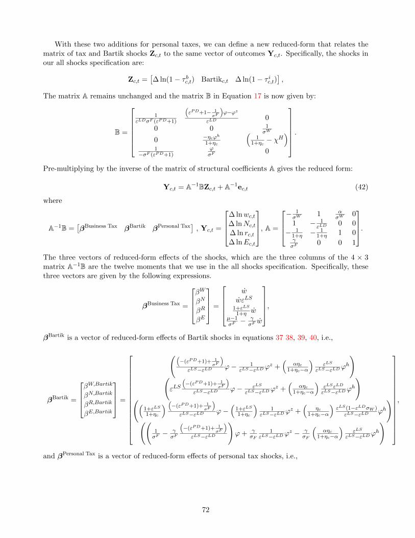
With these two additions for personal taxes, we can define a new reduced-form that relates thematrix of tax and Bartik shocks Zc,t to the same vector of outcomes Yc,t. Specifically, the shocks inour all shocks specification are:

Zc,t =⇥� ln(1� ⌧ bc,t) Bartikc,t � ln(1� ⌧ ic,t)

⇤,

The matrix A remains unchanged and the matrix B in Equation 17 is now given by:

B =

2

666664

1"LD�F ("PD+1)

⇣"PD+1� 1

�F

⌘'�'z

"LD 0

0 0 1�W

0 �⌘c'h

1+⌘c

⇣1

1+⌘c� �H

⌘

1��F ("PD+1)

'�F 0

3

777775.

Pre-multiplying by the inverse of the matrix of structural coe�cients A gives the reduced form:

Yc,t = A�1BZc,t + A�1ec,t (42)

where

A�1B =⇥�Business Tax �Bartik �Personal Tax

⇤, Yc,t =

2

664

� lnwc,t

� lnNc,t

� ln rc,t� lnEc,t

3

775, A =

2

664

� 1�W 1 ↵

�W 01 � 1

"LD 0 0� 1

1+⌘ � 11+⌘ 1 0

��F 0 0 1

3

775.

The three vectors of reduced-form e↵ects of the shocks, which are the three columns of the 4 ⇥ 3matrix A�1B are the twelve moments that we use in the all shocks specification. Specifically, thesethree vectors are given by the following expressions.

�Business Tax =

2

664

�W

�N

�R

�E

3

775 =

2

6664

ww"LS

1+"LS

1+⌘ wµ�1�F � �

�F w

3

7775,

�Bartik is a vector of reduced-form e↵ects of Bartik shocks in equations 37 38, 39, 40, i.e.,

�Bartik =

2

664

�W,Bartik

�N,Bartik

�R,Bartik

�E,Bartik

3

775 =

2

666666666666664

⇣�("PD+1)+ 1

�F

⌘

"LS�"LD '� 1"LS�"LD'z +

⇣↵⌘c

1+⌘c�↵

⌘"LS

"LS�"LD'h

!

"LS

⇣�("PD+1)+ 1

�F

⌘

"LS�"LD '� "LS

"LS�"LD'z +⇣

↵⌘c1+⌘c�↵

⌘"LS"LD

"LS�"LD'h

!

⇣1+"LS

1+⌘c

⌘ ⇣�("PD+1)+ 1

�F

⌘

"LS�"LD '�⇣1+"LS

1+⌘c

⌘1

"LS�"LD'z +⇣

⌘c1+⌘c�↵

⌘"LS(1�"LD�W )

"LS�"LD 'h

!

1�F � �

�F

⇣�("PD+1)+ 1

�F

⌘

"LS�"LD

!'+ �

�F

1"LS�"LD'z � �

�F

⇣↵⌘c

1+⌘c�↵

⌘"LS

"LS�"LD'h

!

3

777777777777775

,

and �Personal Tax is a vector of reduced-form e↵ects of personal tax shocks, i.e.,

72

�Personal Tax =

2

664

�W,Personal Tax

�N,Personal Tax

�R,Personal Tax

�E,Personal Tax

3

775 =

2

6666664

⇣�↵�H(1+⌘)

�F ("LS�"LD)[↵+�W (1+⌘)]� "LS

"LS�"LD

⌘

⇣�"LD[1+⌘+↵(�1+�H(1+⌘))]�F ("LS�"LD)[↵+�W (1+⌘)]

⌘

⇣�H(1+⌘)�"LD[�W (�H⌘��H�1)�1]

("LS�"LD)[↵+�W (1+⌘)]

⌘

⇣��[1+⌘+↵(�1+�H(1+⌘))]�F ("LS�"LD)[↵+�W (1+⌘)]

⌘

3

7777775.

E.5.4 Model Fit

We evaluate the fit of our model by comparing the estimated reduced-form e↵ects to the predictions ofour model. Table A32 presents the estimated reduced-form e↵ects along with the predicted momentsbased on the estimated parameters for three cases. Panel (a) shows the model for the case where onlytaxes are used in estimation and corresponds to Column (1) in Panel (a) of Table 6. In all four cases,the model matches the reduced-form estimates well. However, most of of the e↵ects are not preciselyestimated, with the exception of the e↵ect of taxes on establishment growth. This estimation hasthree parameters and four moments, which allows us to conduct a test of over identifying restrictions.The last line of Panel (a) reports the results of this test and shows that this restriction is not rejectedby the data. Panels (b) and (c) report similar results models corresponding to Columns (1) and (5)of Panel (b) of Table 6, respectively. In both cases the models fit the reduced-form estimates well anddo not reject the over identification restriction. The benefit of using the additional variation in theBartik shock is evident in these panels as the corresponding moments are more precisely estimatedthan those in Panel (a).

E.6 Single-Equation Estimates of Labor Supply, Housing Supply,and Establishment Location

In this subsection, we present a complementary approach to our main estimation methodology byestimating the labor supply, housing supply, and establishment location equations separately. Byisolating each equation, we clarify the potential estimation pitfalls, we show the sources of variationthat we use to overcome these pitfalls, and explore how the structural estimates relate to economicfeatures in our model. By contrast, in our main strategy, we estimate a simultaneous equation modelthat incorporates all of the spatial equilibrium forces of our model. This approach uses classicalminimum distance methods to match the reduced-form e↵ects of business tax changes on equilibriumoutcomes with the prediction from our model. This strategy improves the precision of our estimatesand allows for inference on the incidence to workers, landowners, and firm owners.

E.6.1 Labor Supply

The log of Equation 1 relates changes in labor supply � lnNc,t to changes in wages � lnwc,t, rentalcosts � ln rc,t, and amenities �Ac,t in location c and year t:

� lnNc,t =� lnwc,t � ↵� ln rc,t

�W+

�Ac,t

�W. (43)

where �W is the dispersion of idiosyncratic worker location preferences. We define log real wagechanges, � lnReal Wagec,t ⌘ � lnwc,t � ↵� ln rc,t, where we calibrate ↵ = 0.3 using data form theConsumer Expenditure Survey. In order to implement this equation, consider estimating the followingempirical analogue:

� lnNc,t = �LS� lnReal Wagec,t +D0s,t

LSs,t + ⌫LSc,t (44)

73

where the changes are decadal changes in year t 2 1990, 2000, 2010 are relative to year t� 10, �LS istotal e↵ect of real wage changes, and Ds,t =

⇥I(t = 1990) . . . I(t = 2010) I(Midwest1990)s,t

⇤0is a

vector with year dummies as well as state dummies for states in the industrial Midwest in the 1980s,and ⌫LSc,t is the error term. From Equation 43, it follows that the error term will be composed partlyof aggregate amenity shocks to a given area. Since changes in real wages and changes in amenities arelikely negatively correlated, an OLS estimate of �LS will be biased downwards. Intuitively, rightwardshifts in supply due to amenity improvements result in apparently flatter local labor supply curves.Since �W is related to the inverse of �LS , attenuation in �LS results in overestimates of �W . Inorder to deal with this endogeneity concern, we instrument for real wage changes using the Bartikinstrument for local labor demand as well as changes in taxes � ln(1� ⌧ cc,t). The exclusion restrictionis that workers only value changes in labor demand and corporate taxes only through their e↵ects onthe real wage.78

Table A33 provides estimates for the preference dispersion parameter �W using both OLS andIV approaches. In both cases, we estimate �W as a non-linear function of the estimated �LS usingthe delta method. Comparing Columns (1) and (2), we find that OLS indeed overestimates theparameter �W relative to the IV estimate. Our IV estimate yields a point estimate of �W = 0.72that is significantly di↵erent than zero at the 1% level with a standard error of 0.28. Figure A16depicts the relationship of these estimates to worker mobility. Figure A16 plots the mean log changein population for several bins of log change in real wages as well as the fitted values of a first stageregression of changes in log real wages on the Bartik shock and the tax shock. The fitted lines plotthe associated estimates from OLS and IV regressions and show that the IV estimates imply thatworkers are indeed three times more mobile than the OLS estimates would imply. The IV estimateimplies that a $1 increase in the real wages leads to an increase in population of 1.64. In Section 3.1we discuss how this estimate relates to others in the literature.

E.6.2 Housing Market

The log of housing market clearing condition from Section 1.2 provides the following estimable equa-tion for housing costs:

� ln rc,t = �HM (� lnNc,t +� lnwc,t) +D0s,t

HMs,t + ⌫HM

c,t (45)

where the changes are decadal changes in year t 2 1990, 2000, 2010 relative to year t � 10, Ds,t is avector with year dummies as well as state dummies for states in the industrial midwest in the 1980s,and ⌫HM

c,t is the error term. The structural model implies that �HM = 11+⌘ , the average elasticity of

housing supply.As discussed in the previous section, the error term in this equation is partly composed of pro-

ductivity shocks to the housing sector. To the extent that these shocks are positively correlated withchanges in population, we would expect that OLS estimates of the coe�cient �HM might be biased.We avoid this potential issue by estimating this equation via IV, where we instrument for changesin population and wages using corporate tax changes and Bartik productivity shocks. As before, wereport estimates of the parameter ⌘ from a delta method calculation.

Table A33 provides estimates for ⌘. Column (3) provides the OLS estimate and Column (4)provides the IV estimate, which gives a similar, though slightly smaller estimate of the elasticity ofhousing supply of 0.834(SE = 0.432). The parameter implies that a 1% increase in population orwages would raise rental costs by 0.55%(SE = 0.12), which is a statistically significant e↵ect at the99% level. While not perfectly comparable to previous estimates, this estimate is within the range

78In order to ensure that this is the case, we control for changes in state personal income taxes that might drive boththe location of establishments and workers.

74

of parameters from previous studies including those in Notowidigdo (2013) and Suarez Serrato andWingender (2011).79

E.6.3 Establishment Location and Labor Demand

Log di↵erencing Equation 7 we obtain the following equation:

� lnEc,t =

✓µ� 1

�F� �

�Fw

◆

| {z }�ES

� ln(1� ⌧ bc,t) +D0s,t

ESs,t + ⌫ES

c,t .

To observe the interpretation of the coe�cient �ES as a combination of direct and indirect e↵ects,consider first estimating the following alternative equation for establishment share growth:

� lnEc,t = �ES� ln(1� ⌧ bc,t) + �ES2 � lnwc,t +D0

s,t ESs,t + ⌫ES

c,t . (46)

If both changes in wages and changes in taxes are exogenous, Equation 46 shows that �ES would berelated to 1

�("PD+1)�F and that a coe�cient on wages �ES2 would be related to �

� ��F

�. The key issue

in estimating this equation is that the structural error term, i.e. the change in common productivity�Bc,t, is likely positively correlated with wages. This omitted variable would likely bias an OLSestimation and produce estimates of the output elasticity of labor � that are negative, contrary toany plausible economic model. Indeed, Column (5) of Table A33 presents the implied estimates fromsuch a regression. As predicted, this estimation yields a non-sensical, negative estimate of the outputelasticity of labor �, which would imply an up-ward sloping labor demand curve.

In order to deal with this endogeneity problem we exclude the endogenous regressor � lnwc,t (i.e.,we impose the constraint that �ES

2 = 0). This exclusion, however, changes the interpretation ofthe parameter �ES . This estimate corresponds to the reduced form e↵ects of a business tax cut onestablishment growth as reported in Table 4, Column 4. The estimation of the parameter �F fromthis equation is presented in Section E.6.4.

E.6.4 CMD Estimation of the Establishment Location Equation

Estimating labor demand functions in models of local labor markets has been limited by the lack ofplausibly exogenous labor supply shocks that may trace the slope of the demand function.80 Instead,this equation exploits the empirical tradeo↵ firms make among productivity, corporate taxes, andfactor prices to recover the parameters governing labor demand and the incidence on firm profits.

Recall from Section 3.1 that the exact reduced-form of the establishment location equation isgiven by:

� lnEc,t =

✓µ� 1

�F� �

�Fw

◆

| {z }�E

� ln(1� ⌧ bc,t) +D0s,t

4s,t + u4c,t.

79Our housing supply elasticity parameter and corresponding estimates are not directly comparable due to our model’sassumption of Cobb Douglas housing demand rather than the assumption that each household inelastically demandsone unit of housing. This feature makes rent a function of both wages and population rather than just population andslightly alters the functional form. We adopt the Cobb-Douglas assumption to allow households to adjust to shocks overthe long run, but this feature is not an essential part of our model or results. In an earlier version of the paper, we usedinelastic demand and found similar results to those reported here.

80Recent papers have used structural approaches to ensuring a downward-sloping labor demand curve (e.g., No-towidigdo (2013)) or have emphasized the role of local amenities in driving relative demand for skilled and unskilledworkers (e.g., Suarez Serrato and Wingender (2011) and Diamond (2012)).

75

While we derived this equation from the SEM, this equation can also be obtained by log di↵erencingEquation 7. We can decompose the parameter �E into two forces: the increased desirability of alocation through lower taxes and the countervailing force of higher wages:

m(✓) ⌘ 1

�("PD + 1)�F

| {z }LowerTaxes

�⇣ �

�F

⌘w(✓)

| {z }Higher Wages

(47)

where w(✓) is given in Equation 10 and ✓ is the vector of parameters of the model. Thus, given theparameters of the model ⌘,�W , "PD, and � and an estimated �E , one can recover an estimate of theproductivity dispersion parameter �F .

Formally, we recover the estimate of �F via classical minimum distance. We first estimate �E viaOLS. Using the parameter �E as an empirical moment of the data along with its respective varianceV, the classical minimum distance estimator is the solution to Equation 22 where m(✓) is as inEquation 47. This approach takes calibrated values of the parameters ⌘,�W , "PD, and �, finds thevalue �F that solves Equation 22 and computes its variance.

Figure A17 shows estimates for �F from the CMD estimation using the values for calibratedparameters discussed above. The graph plots the mean values of log changes in the number ofestablishments for di↵erent bins of log changes in the net of business tax rate. The red line plotsthe relation between changes in taxes and firm mobility that is implied by the CMD estimation.The parameter estimate in this case is �F = 0.1(SE = 0.058), which is statistically significant. Theblack line plots the same relationship when we use an implied value of �F from an OLS regressionthat ignores the indirect e↵ect of tax cuts on firm location through higher wages. The red line issteeper than the black line, which makes firms look more mobile than they would appear in the OLSspecification and is consistent with the fact that the CMD estimate is three times smaller than theimplied value from the OLS regression.81 However, if we consider the conventional wisdom of perfectmobility as given by the vertical green line, we see that even a small value of productivity dispersion�F yields estimates of firm mobility that are far smaller than that implied by the conventional wisdom.

F Accounting for Changes in Government Spending

We follow Suarez Serrato and Wingender (2011) in modeling the e↵ects of changes in governmentspending on the local economy. This modeling approach takes into account the e↵ects of changes inlabor demand from government, changes in the provision of public goods, and changes in the provisionof infrastructure.

Consider first the e↵ects of changes on the welfare of workers. Extending the indirect utilityfunction to account for government services GS, we have:

V Wnc = a0 + lnwc � ↵ ln rc + � lnGSc + lnAnc,

where � is the worker’s valuation of government services. Including a direct e↵ect of governmentservices on utility leads to a naturally extension of Equation 13 for the welfare e↵ects of a change incorporate taxes:

dVW

d ln(1� ⌧ cc )= Nc(wc � ↵rc + �GSc),

where VW = E"[maxc V Wnc ]. Implementing this equation requires two pieces of data: the valuation of

81The results of these regressions are also presented in table form in Table A33.

76

government services � and the change in services provided. We use the results from Suarez Serratoand Wingender (2011) with an estimate of � = 0.45.82 Government services are provided by localworkers such that GSc is determined by changes in expenditure on services as well as changes in thewages of local workers. That is, GSc = ExpGS

c � wc. We implement this equation empirically with:

�W � ↵�R + �(ExpGSc � �W ).

A key thing to note from this equation is that workers care about the e↵ects of the policy changeon their real income lnwc�↵ ln rc and that the equilibrium change in this quantity equals �W �↵�R

regardless of whether this change is due to increases in the demand of workers or changes in thesupply of workers due to changes in government spending. For the same reason, the incidence onlandowners is still given by rc = �R.

Consider now the e↵ects of changing infrastructure spending on the profits of firms. We modelinfrastructure as a component of productivity by decomposing the productivity shock Bc = BcZ

⌫ ,where Zc is infrastructure and ⌫ is the firms’ output elasticity of infrastructure. If changes in revenuefrom a change in the corporate tax rate result in changes in infrastructure spending, then the e↵ect onfirm profits can be quantified as a combined change in taxes and an infrastructure-based productivityshock. Following the incidence equations for a productivity shock in Appendix B.4, the combinede↵ects of a tax change on profit is:

⇡c +

2

66664�("PD + 1)| {z }

Direct E↵ect on ⇡

+ �("PD + 1)⇥

1�F � ("PD + 1)

"LS � "LD

!

| {z }E↵ect of Wage Change on ⇡

3

77775⇥ ⌫Zc|{z}

Size of Productivity Shock

,

where ⇡c is as given in Equation 14. Implementing this equation requires parameters from our struc-tural estimates as well as two additional pieces of data: the firms’ output elasticity of infrastructure⌫ and the change in infrastructure spending. We use the results form Suarez Serrato and Wingender(2011) with an average estimate of ⌫ = 0.27.83 Infrastructure Zc is assumed to be imported and doesnot require the hiring of local workers so that Zc = ExpZc .

We require an estimate of the e↵ects of a tax cut on revenue in order to implement these equationsrequires. Since the average share of corporate taxes revenue to income tax revenue is approximately20%, a static forecast of the change in revenue following a 1% tax cut would be -.2%. Given that taxcuts lead to increases in economic activity, the static estimate would be a lower bound on the e↵ectson revenue. We thus assume that the change in revenue following a 1% tax cut would be -.1%.

We implement these expanded incidence equations under three alternative scenarios about howthe change in revenues a↵ects expenditures on infrastructure and expenditure on government services.The first scenario assumes that, following a tax cut, the decrease in revenue will be used to decreasegovernment services. The second scenario assumes that the associated decrease in revenue will be usedto decrease the provision of infrastructure. The third and final scenario assumes that the decrease inrevenue will be used to decrease both government services and infrastructure proportionally.

Table A2 presents the results from this exercise. Column (1) presents our baseline results thatdo not account for changes in government spending. Column (2) assumes that all of the change in

82Suarez Serrato and Wingender (2011) estimate the value of government services for skilled and unskilled workers.The value we use in our calculations is the average of these two value assuming an average share of skilled workers of25%.

83Suarez Serrato and Wingender (2011) estimate the output elasticity of infrastructure for the labor demand of skilledand unskilled workers. The value we use in our calculations is the average of these two value assuming an average shareof skilled workers of 25%.

77

revenue a↵ects changes in the provision of government services. We use an average share of spendingon services to individuals of 90% following data from the Annual Survey of State Finances from2013. This implies that a 1% drop in revenue lowers expenditures on public goods by 1.11%. In thisscenario, the decrease in government services lowers worker utility resulting in smaller share of thetotal benefits of 18%. Column (3) explores the e↵ect of decreasing infrastructure on firm profits. Inthis case, since only 10% of spending is assumed to be infrastructure related, a 1% drop in revenuelowers infrastructure spending by 10%. We observe that the incidence in firm profits falls to 0.71from 0.81. However, this decrease in profits only lowers the share of incidence accruing to firm ownersto 41%. Finally, consider the case where the decrease in revenue is apportioned proportionally sothat a 1% fall in revenue implies a 1% decline in spending in each category. Column (4) present theincidence resulting form this scenario. We observe that firm profits are only modestly a↵ected whileworker welfare sees a steeper decline. Relative to the baseline case, we observe that the result thatfirm owners bear a substantial portion of the benefit of a corporate tax cut is only strengthened byaccounting for the e↵ects on government spending.

Table A2: Incidence Estimates Accounting for Government Spending

(1) (2) (3) (4)

Assumptions for AnalysisValue of Government Services N Y N YValue for Infrastructure N N Y YChange in Funds None Services Infrastructure Proportional

IncidenceLandowners 0.32 0.32 0.32 0.32Workers 0.68 0.25 0.68 0.29Firm Owners 0.81 0.81 0.71 0.8

Share of IncidenceLandowners 18% 23% 19% 23%Workers 38% 18% 40% 21%Firm Owners 45% 59% 41% 57%

G Accounting for Changes in Local Prices

This section amends the model and incidence estimates to account for changes in local prices (i.e.,the price of non-housing, non-traded goods). We present modified incidence expressions and discusshow the results change. We then provide additional detail on how we amend the demand and supplycomponents of the model to derive the modified incidence expressions.

G.1 Incidence Estimates that Account for Non-traded Goods

With local goods, the welfare e↵ects of a tax cut in location c on the welfare of workers are similar tothe expression in equation 13. The part of the expression that accounts for local increases in rental

78

prices, (↵rc), is replaced with (↵H rc + ↵NT pNTc ):

dVW

d ln(1� ⌧ cc )=Nc(wc � ↵H rc + ↵NT pNT

c ) (48)

=Nc(�W � ↵H�R + ↵NT�NT ), (49)

where ↵H is the expenditure share on housing and ↵NT is the expenditure share on non-housing,non-traded goods. For firm owners and landowners, the expressions are the same as in 14 and 15.84

We implement these modified incidence expressions in four ways. First, we use the local priceindex from ACCRA instead of �R in our baseline approach, i.e., the welfare for workers is measuredas follows: �W � .3�P,ACCRA. Mian and Sufi (2016) show that on an employment basis in their maintrade-based classification of industries, non-tradable industries account for 20% of employment andconstruction accounts for 11% of employment. However, other work uses larger shares for expenditureon local goods. In the second implementation, we consider a larger value of ↵ = .6 from Beraja,Hurst and Ospina (2016).85 In this case, the incidence expression for workers is �W � .6�P,ACCRA.Third, we split local goods into housing and non-traded, non-housing goods using local expenditureshares from Beraja, Hurst and Ospina (2016), resulting in the following expression for worker welfare:�W � .2�P,ACCRA,residual� .4�P,ACCRA,NT where �P,ACCRA,residual is the reduced-form impact on theportion of the local price index that is not categorized as non-traded. It is calculated using weights inthe ACCRA formulas that put .47 on the items in �P,ACCRA,NT , which implies �P,ACCRA,residual =�P,ACCRA�.47⇥�P,ACCRA,NT

(1�.47) . Finally, for the fourth importation, we use a di↵erent measure of local

prices from the BLS and measure the welfare e↵ects for workers as �W � .3�P,BLS .Table A3 shows the results of accounting for local prices. We find similar estimates to our baseline

results when accounting for changes in local prices. Columns (1)-(4) implement the four approachesusing the reduced-form e↵ects of local business tax cuts that control for Bartik; Columns (5)-(8)implement the same four approaches using the reduced-form e↵ects that do not control for Bartik(i.e., column (1) of the reduced-form outcome tables). In particular, Column (1) shows the incidenceon workers is .78 � .3 ⇥ .16 = .73 where .78 is from the Bartik specification (i.e., Column (4)) inTable A7 and .16 is from the Bartik specification in Table A12. Column (2) uses a higher value of ↵,but the same reduced-form e↵ects as the first column, resulting in a slightly lower impact on workersof, .78 � .6 ⇥ .16 = .68. Column (3) shows that separating local goods into a non-traded group anda residual produces similar results. We use the reduced-form impacts from Tables A12 and A13 toimplement the third approach: �W � .2�P,ACCRA,residual� .4�P,ACCRA,NT = .78� .2⇥ .28� .4⇥ .02 =.66.86 Finally, Column (4) uses a di↵erent measure of local prices PBLS , for which the reduced-formimpacts are reported in Table A14. This alternative measure is notably similar to our baseline thatuses the change in rental prices. Columns (5)-(8) repeat the same calculations using slightly di↵erentinputs from the respective reduced-form tables. Overall, local price increases are modest over a tenyear period. Accounting for these impacts results in similar incidence results to our baseline estimates.

84We also show below (in section G.2.2) that we can use ⇡c = 1 + ˙AvgSalesc to measure incidence in terms of salesrather than in terms of cost. The resulting estimates are similar (e.g., compare the estimate from Column (1) in TableA15 with the incidence estimates on firm owners that use reduced-form estimates from the same specification such asthose in Column (1) of Table 5). We primarily focus on the cost-based estimates for firm owners since they are moreprecise than those in Table A15, but these results provide further support for the conclusion that firm owners bear asubstantial share of the incidence of business tax cuts.

85See Tables A24 and A25 for our baseline specification for ↵ = .5 and ↵ = .65, respectively.86Note that .28 = �P,ACCRA,residual = �P,ACCRA�.47⇥�P,ACCRA,NT

(1�.47).

79

Table A3: Incidence Estimates Accounting for Changes in Local Prices

A. Using Reduced-Form Estimates w/ Bartik Controls B. Using Reduced-Form Estimates w/o Bartik Controls(1) (2) (3) (4) (5) (6) (7) (8)

IncidenceLandowners 0.32 0.32 0.32 0.32 1.17 1.17 1.17 1.17Workers 0.73 0.68 0.66 0.52 1.34 1.22 1.18 1.08Firm Owners 0.81 0.81 0.81 0.81 1.63 1.63 1.63 1.63

Share of IncidenceLandowners 17.2% 17.6% 17.9% 19.4% 28.3% 29.1% 29.4% 30.2%Workers 39.3% 37.7% 37.0% 31.6% 32.3% 30.4% 29.7% 27.7%Firm Owners 43.5% 44.7% 45.2% 49.0% 39.4% 40.5% 41.0% 42.1%

Local Price Index PACCRA PACCRA PACCRA,NT PBLS PACCRA PACCRA PACCRA,NT PBLS

Parameters↵ 0.3 0.6 0.3 0.3 0.6 0.3↵H 0.2 0.2↵NT 0.4 0.4

Notes: This table shows incidence of local business tax changes over ten years on landowners, firm owners, and workings using di↵erent measures of local prices.

Local price data are described in Appendix A.4. The first four columns show incidence results based on reduced-form estimates from Column 4 in Table 4-type tables,

which controls for Bartik, for all the relevant outcomes in the incidence expressions in equations 48, 14, and 15. The last four columns repeat the same specifications

but use the reduced-form estimates from Column 1 in Table 4-type tables, which does not control for Bartik. Specifically, Column (1) and (5) calculate the incidence

on workers by taking the di↵erence between the reduced-form impact on wages and ↵�P,ACCRA from Tables A7 and A12. For example, the worker estimate in

Column (1), which corresponds to the specification controlling for Bartik, is �W � ↵�P,ACCRA = .78 � .3 ⇥ .16 = .73 and for Column (5), which corresponds to the

specification not controlling for Bartik, is �W � ↵�P,ACCRA = 1.45 � .3 ⇥ .38 = 1.34. Column (2) and (6) use an ↵ of .6 instead of .3. Columns (3) and (7) break

out traded and non-traded ACCRA price indexes and to present estimates of �W � .2�P,ACCRA,residual + .4�P,ACCRA,NT where �P,ACCRA,residual is the ACCRA

local price index on items not covered in the NT index. It is calculated using weights in the ACCRA formulas that put .47 on the items in �P,ACCRA,NT , which

implies �P,ACCRA,residual = �P,ACCRA�.47⇥�P,ACCRA,NT

(1�.47). These estimates are from Tables A12 and A13. The expenditure weight of .6, which is divided into .2 and

.4, is based on estimates from Beraja, Hurst and Ospina (2016) on the share of total local consumption (.6) and the share of housing consumption (.2), which they

assume is entirely local. Finally, Columns (4) and (8) use an alternative local price index from BLS, which isn’t available for all locations but covers a large share of

the population. In particular, the estimates for workers are �W � ↵�P,BLS and the reduced-form estimates for local prices �P,BLS are in Table A14.

80

G.2 Deriving Incidence Expressions that Account for Non-traded Goods

G.2.1 Demand with Non-traded Goods

In location c with amenities A, households maximize Cobb-Douglas utility over housing h, a compositeXNT of local (non-housing non-traded) goods xNT

j , a composite X of tradable goods xj while facing

a wage w, rent r, local good prices pNTj , and traded good prices pj :

maxh,xNT ,X

lnA+ ↵H lnh+ ↵NT lnXNT + (1� ↵H � ↵NT ) lnX s.t. rh+X

j2JNT

pNTj xNT

j +X

j2Jpjxjdj = w,

where XNT =

P

j2JNT

(xNTj )

✏PD,NT+1

✏PD,NT dj

! ✏PD,NT

✏PD,NT+1

, X =

Pj2J

x"PD+1

"PD

j dj

! "PD

"PD+1

, and ✏PD,NT < �1

is the product demand elasticity of local goods.Demand from each household for local variety j in location c is:

xNTjc = (pNT

jc )✏PD,NT

INTc (PNT

jc )1+✏PD,NT(50)

where PNTc =

P

j2JNTc

ENTc (pNT

jc )1+"PD

! 1

1+"PD

, ENTc is the number of non-traded establishments,

and INTc = ↵NTNcwc is total expenditures on local goods.

G.2.2 Supply of Non-traded Goods

Similar to the baseline firm problem, establishments in location c maximize profits over inputs andprices pNT

jc while facing a local wage wc, national rental rates ⇢, national prices pv of each variety v,

and local business taxes ⌧ bc subject to the production technology in Equation 3:

⇡NTjc = max

ljc,kjc,xv,jc,pNTjc

(1� ⌧ bc )

0

@pNTjc xNT

jc � wcljc �Z

v2J

pvxv,jcdv

1

A� ⇢kjc, (51)

Following the same input demand steps in appendix B.2, we can relate sales to unit costs:

pNTj xNT

j| {z }⌘SalesNT

jc

= xNTj µNT 1

Bjc

hw�⇢�������(1� � � �)�(1����)

i

| {z }⌘cjc

(52)

This expression shows that local prices are a fixed-mark up over unit costs, pNTj = µNT cjc where the

markup on local goods µNT ⌘⇥

1"PD,NT + 1

⇤�1is constant due to CES demand. Since local prices are

81

a fixed-mark up over unit costs, we can express after tax profits as follows:

⇡NTjc = (1� ⌧ bc )

�pNTjc � cjc

�xNTjc (53)

⇡NTjc = (1� ⌧ bc )

�pNTjc � cjc

� SalesNTjc

pNTjc

(54)

⇡NTjc = (1� ⌧ bc )

�µNT cjc � cjc

� SalesNTjc

µNT cjc(55)

⇡NTjc = (1� ⌧ bc )

SalesNTjc

�"PD,NT(56)

where the second line comes from the definition of sales, the third line comes from the relationshipbetween prices and costs (from equation 52) and the fourth line comes from the definition of themarkup. Similar steps imply that we can express after tax profits for traded-establishments as ⇡T

jc =

(1� ⌧ bc )Salesjc�"PD,T .

Therefore total after-tax firm profits is:

ETc ⇡

Tjc + ENT

c ⇡NTjc = (1� ⌧ bc )

ET

c

AvgSalesTjc�"PD,T

+ ENTc

AvgSalesNTjc

�"PD,NT

!(57)

= (1� ⌧ bc )

✓TotSalesTc�"PD,T

+TotSalesNT

c

�"PD,NT

◆(58)

= (1� ⌧ bc )TotSalesc

✓TotSalesTcTotSalesc

1

�"PD,T+

TotSalesNTc

TotSalesc

1

�"PD,NT

◆(59)

This expression shows that total sales changes reveal information about changes in total profits. Inthe simple case in which the product demand elasticities are the same, then the term in parenthesis is

1�"PD and the average after-tax profit per establishment is: ⇡T

c = (1� ⌧ bc )⇣AvgSalesc

�"PD

⌘. In the case in

which the product demand elasticities are di↵erent, the term in parenthesis will be constant (since thesales shares will be constant due to Cobb Douglas preferences and production technology.) Therefore,in both cases, ⇡c = 1 + ˙AvgSalesc. We can use this expression to quantity ⇡c when there are bothtraded and non-traded goods.

82

Table A4: Correlation in State Tax Rates

A. Tax Rates⌧ cs ⌧ saless ⌧ is ⌧props

⌧ cs 1.000⌧ saless 0.008 1.000⌧ is 0.323 -0.257 1.000⌧props 0.113 -0.030 0.012 1.000

B. 10 Year Di↵erences in Tax Rates�⌧ cs �⌧ saless �⌧ is �⌧props

�⌧ cs 1.000�⌧ saless 0.315 1.000�⌧ is 0.078 -0.007 1.000�⌧props -0.046 -0.191 -0.176 1.000

Notes: This table shows the correlation between tax rates in levels (in Panel A) and changes (in Panel B). See Section 4

for data sources for ⌧ corps and ⌧ i

s. State sales tax rates come from the Book of the States, Table 7.10. The variable is

the general sales and gross receipts tax (percent). For property taxes, we use U.S. Censuses as well as the 2009 ACS to

obtain an estimate of average property tax liability at the state level. The ratio of these tax liabilities to self reported

home values is our estimate of the property tax rate.

83

Table A5: Annual E↵ects of Business Tax Cuts on Establishment GrowthEstablishment Growth (1) (2) (3) (4) (5) (6) (7)

� Log Net-of-Business-Taxt 0.11 0.16 -0.04 0.19 0.42 0.20 0.27(0.16) (0.21) (0.24) (0.18) (0.26) (0.30) (0.38)

� Log Net-of-Business-Taxt�1 0.14 0.36 0.36 0.14 0.47* 0.54** 0.59(0.13) (0.22) (0.23) (0.14) (0.27) (0.27) (0.39)

� Log Net-of-Business-Taxt�2 0.48*** 0.50** 0.51** 0.52** 0.54** 0.61** 0.63(0.17) (0.20) (0.24) (0.20) (0.25) (0.29) (0.38)

� Log Net-of-Business-Taxt�3 0.57*** 0.55** 0.58** 0.57** 0.55* 0.62* 0.50(0.20) (0.23) (0.25) (0.22) (0.28) (0.31) (0.34)

� Log Net-of-Business-Taxt�4 0.20 0.19 0.17 0.15 0.16 0.17 0.13(0.13) (0.13) (0.16) (0.25) (0.30) (0.34) (0.37)

� Log Net-of-Business-Taxt�5 0.02 0.03 -0.00 0.19 0.25 0.25 0.21(0.25) (0.26) (0.26) (0.32) (0.37) (0.38) (0.41)

� Log Net-of-Business-Taxt�6 0.18 0.22 0.26 0.30(0.25) (0.31) (0.31) (0.36)

� Log Net-of-Business-Taxt�7 0.34** 0.43* 0.33 0.46*(0.16) (0.23) (0.23) (0.26)

� Log Net-of-Business-Taxt�8 0.21 0.21 0.15 0.26(0.13) (0.17) (0.18) (0.18)

� Log Net-of-Business-Taxt�9 0.03 0.01 0.04 0.02(0.14) (0.15) (0.16) (0.17)

� Log Net-of-Business-Taxt�10 0.26 0.25 0.32* 0.31*(0.16) (0.16) (0.16) (0.18)

� Log Net-of-Business-Taxt+1 0.10 0.03 0.13 0.20 0.02(0.20) (0.20) (0.22) (0.23) (0.30)

� Log Net-of-Business-Taxt+2 -0.02 0.22 -0.06 0.30 0.08(0.16) (0.20) (0.18) (0.23) (0.31)

� Log Net-of-Business-Taxt+3 -0.10 0.04 -0.05(0.32) (0.33) (0.40)

� Log Net-of-Business-Taxt+4 -0.33 -0.36 -0.30(0.22) (0.25) (0.45)

� Log Net-of-Business-Taxt+5 -0.33 -0.39 -0.28(0.23) (0.27) (0.42)

� Log Net-of-Business-Taxt+6 -0.15(0.33)

� Log Net-of-Business-Taxt+7 -0.30(0.38)

� Log Net-of-Business-Taxt+8 -0.30(0.33)

� Log Net-of-Business-Taxt+9 -0.05(0.11)

� Log Net-of-Business-Taxt+10 -0.11(0.13)

Observations 13,230 12,250 10,780 10,780 9,800 8,330 5,880R-squared 0.225 0.143 0.099 0.197 0.106 0.054 0.120Cumulative E↵ect over 5 Years 1.51** 1.80* 1.59 1.77* 2.38 2.39 2.34

(0.75) (1.02) (1.14) (1.03) (1.58) (1.72) (2.10)Cumulative E↵ect over 10 Years 2.79* 3.49 3.49 3.70

(1.51) (2.27) (2.36) (2.81)P-value of All Lags=0: 0.003 0.012 0.051 0.000 0.002 0.037 0.036P-value of All Leads=0: 0.74 0.40 0.66 0.46 0.92

Notes: This table shows the e↵ects of annual local business tax cuts on local establishment growth. Data are for

490 county-groups. See Section 4 for sources. Cumulative e↵ects and F-stats of joint tests that all leads and lags are

zero indicate that tax cuts increase local establishment growth and do not exhibit statistically non-zero pre-trends.

Regressions use initial population as weights and include year fixed e↵ects and dummies for states in the industrial

midwest in the 1980s. Standard errors clustered by state are in parentheses and *** p<0.01, ** p<0.05, * p<0.1.

84

Table A6: E↵ects of Business Tax Cuts on Population Growth over 10 Years

Population Growth (1) (2) (3) (4) (5) (6)

� ln(1� ⌧ b) 4.28** 4.29** 4.25** 3.74** 4.11** 3.53**(1.65) (1.66) (1.66) (1.48) (1.59) (1.47)

�ITC -0.09 0.19(0.25) (0.25)

� lnGOVEXPEND PER CAPITA -0.01 -0.01(0.01) (0.01)

Bartik 0.44** 0.44**(0.19) (0.17)

� ln(1� ⌧EXT ) -4.70*** -4.74***(1.70) (1.63)

Constant 0.07*** 0.07*** 0.07*** 0.02 0.08*** 0.03(0.02) (0.02) (0.02) (0.02) (0.02) (0.02)

Observations 1,470 1,470 1,470 1,470 1,470 1,470R-squared 0.112 0.112 0.115 0.138 0.135 0.164

Notes: See notes from Table 4.

85

Table A7: E↵ects of Business Tax Cuts on Wage Growth over 10 Years

Wage Growth (1) (2) (3) (4) (5) (6)

� ln(1� ⌧ b) 1.45 1.50 1.45 0.78 1.42 0.82(0.94) (0.94) (0.95) (0.82) (0.96) (0.84)

�ITC -0.37** -0.23(0.15) (0.16)

� lnGOVEXPEND PER CAPITA 0.00 0.00(0.00) (0.00)

Bartik 0.56*** 0.54***(0.08) (0.08)

� ln(1� ⌧EXT ) -0.98 -0.44(1.02) (0.79)

Constant -0.09*** -0.09*** -0.09*** -0.14*** -0.09*** -0.14***(0.01) (0.01) (0.01) (0.01) (0.01) (0.01)

Observations 1,470 1,470 1,470 1,470 1,470 1,470R-squared 0.402 0.414 0.402 0.490 0.404 0.495

Notes: See notes from Table 4.

86

Table A8: E↵ects of Business Tax Cuts on Rental Cost Growth over 10 Years

Rental Cost Growth (1) (2) (3) (4) (5) (6)

� ln(1� ⌧ b) 1.17 1.33 1.17 0.32 1.02 0.43(1.44) (1.40) (1.44) (1.37) (1.48) (1.36)

�ITC -1.13** -0.88*(0.55) (0.50)

� lnGOVEXPEND PER CAPITA -0.00 -0.00(0.01) (0.01)

Bartik 0.70** 0.63***(0.27) (0.23)

� ln(1� ⌧EXT ) -4.25* -2.83*(2.39) (1.58)

Constant 0.08*** 0.08*** 0.08*** 0.01 0.09*** 0.03(0.01) (0.01) (0.01) (0.03) (0.01) (0.03)

Observations 1,470 1,470 1,470 1,470 1,470 1,470R-squared 0.139 0.177 0.139 0.189 0.153 0.223

Notes: See notes from Table 4.

87

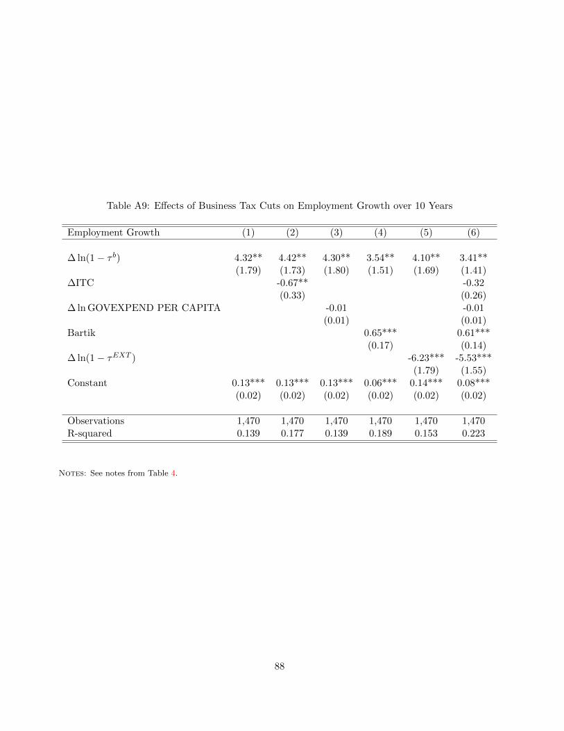
Table A9: E↵ects of Business Tax Cuts on Employment Growth over 10 Years

Employment Growth (1) (2) (3) (4) (5) (6)

� ln(1� ⌧ b) 4.32** 4.42** 4.30** 3.54** 4.10** 3.41**(1.79) (1.73) (1.80) (1.51) (1.69) (1.41)

�ITC -0.67** -0.32(0.33) (0.26)

� lnGOVEXPEND PER CAPITA -0.01 -0.01(0.01) (0.01)

Bartik 0.65*** 0.61***(0.17) (0.14)

� ln(1� ⌧EXT ) -6.23*** -5.53***(1.79) (1.55)

Constant 0.13*** 0.13*** 0.13*** 0.06*** 0.14*** 0.08***(0.02) (0.02) (0.02) (0.02) (0.02) (0.02)

Observations 1,470 1,470 1,470 1,470 1,470 1,470R-squared 0.139 0.177 0.139 0.189 0.153 0.223

Notes: See notes from Table 4.

88

Table A10: E↵ects of Business Tax Cuts on Growth in GOS per Establishment over 10 Years

Growth in GOS per establishment (1) (2) (3) (4) (5) (6)

� ln Net-of-Business-Tax Rate 4.07** 3.92* 4.08* 3.66* 4.20** 3.50*(2.02) (2.02) (2.03) (2.00) (1.95) (1.95)

� State ITC 1.05*** 1.06***(0.27) (0.32)

� lnGov. Expend./Capita 0.00 0.00(0.00) (0.00)

Bartik 0.34 0.42*(0.22) (0.22)

Change in Other States’ Taxes 3.63 2.47(2.33) (2.21)

Observations 1,470 1,470 1,470 1,470 1,470 1,470R-squared 0.138 0.172 0.138 0.150 0.149 0.196

Notes: This table shows the e↵ects of local business tax changes over ten years on gross operating surplus (GOS) per

establishment. The data are decade changes from 1980-1990, 1990-2000, and 2000-2010 for 490 county-groups. GOS

data are from BEA regional statistics. See Section 4 for other data sources used in the table. The specifications are

exactly the same as in Table 4. Standard errors clustered by state are in parentheses and *** p<0.01, ** p<0.05, *

p<0.1.

89

Table A11: E↵ects of Business Tax Cuts on Growth in Sales Tax Revenue over 10 Years

Growth in sales tax revenue per establishment (1) (2) (3) (4) (5) (6)

� ln Net-of-Business-Tax Rate 2.26 2.24 2.27 2.27 2.16 2.15(3.42) (3.43) (3.42) (3.44) (3.37) (3.41)

� State ITC 0.09 0.23(0.33) (0.31)

� lnGov. Expend./Capita 0.01 0.01(0.01) (0.01)

Bartik -0.01 -0.01(0.30) (0.30)

Change in Other States’ Taxes -3.82 -4.12(2.57) (2.47)

Observations 1,422 1,422 1,422 1,422 1,422 1,422R-squared 0.539 0.539 0.539 0.539 0.543 0.544

Notes: This table shows the e↵ects of local business tax changes over ten years on state sales tax revenue per establish-

ment. The data are decade changes from 1980-1990, 1990-2000, and 2000-2010 for 490 county-groups, but not all states

collect sales taxes so the number of observations has 16 fewer county-groups per decade. Sales tax revenue is from the

census of governments. See Section 4 for other data sources used in the table. The specifications are exactly the same

as in Table 4. Standard errors clustered by state are in parentheses and *** p<0.01, ** p<0.05, * p<0.1.

90

Table A12: E↵ects of Business Tax Cuts on Growth in Local Price Index (ACCRA) over 10 Years

Growth in Price Index (ACCRA) (1) (2) (3) (4) (5) (6)

� ln Net-of-Business-Tax Rate 0.38 0.36 0.38 0.16 0.29 0.01(1.39) (1.38) (1.39) (1.51) (1.43) (1.55)

� State ITC 0.20 0.33(0.19) (0.21)

� lnGov. Expend./Capita -0.00 -0.00(0.00) (0.00)

Bartik 0.22* 0.23**(0.11) (0.11)

Change in Other States’ Taxes -2.12 -2.34(1.79) (1.76)

Observations 1,201 1,201 1,201 1,201 1,201 1,201R-squared 0.119 0.121 0.119 0.129 0.127 0.142

Notes: This table shows the e↵ects of local business tax changes over ten years on growth in the ACCRA price index.

The data are decade changes from 1980-1990, 1990-2000, and 2000-2010 for 490 county-groups, but some local areas are

not covered by ACCRA. See Appendix A.4 for data details on local prices and Section 4 for other data sources. The

specifications are exactly the same as in Table 4. Standard errors clustered by state are in parentheses and *** p<0.01,

** p<0.05, * p<0.1.

91

Table A13: E↵ects of Business Tax Cuts on Growth in Local Non-traded Price Index (ACCRA) over10 Years

Growth in Local Non-traded Price Index (ACCRA) (1) (2) (3) (4) (5) (6)

� ln Net-of-Business-Tax Rate 0.11 0.08 0.12 0.02 0.10 -0.06(0.88) (0.86) (0.88) (0.91) (0.89) (0.92)

� State ITC 0.34** 0.39**(0.15) (0.15)

� lnGov. Expend./Capita 0.00 0.00(0.00) (0.00)

Bartik 0.09 0.11**(0.06) (0.05)

Change in Other States’ Taxes -0.33 -0.63(1.24) (1.07)

Observations 1,201 1,201 1,201 1,201 1,201 1,201R-squared 0.055 0.068 0.056 0.058 0.055 0.076

Notes: This table shows the e↵ects of local business tax changes over ten years on growth in the ACCRA non-traded

price index. The data are decade changes from 1980-1990, 1990-2000, and 2000-2010 for 490 county-groups, but some

local areas are not covered by ACCRA. See Appendix A.4 for data details on local prices and Section 4 for other data

sources The specifications are exactly the same as in Table 4. Standard errors clustered by state are in parentheses and

*** p<0.01, ** p<0.05, * p<0.1.

92

Table A14: E↵ects of Business Tax Cuts on Growth in Local Price Index (BLS) over 10 Years

Growth in Local Price Index (BLS) (1) (2) (3) (4) (5) (6)

� ln Net-of-Business-Tax Rate 1.25 1.35 1.27 0.86 1.19 1.06(0.92) (0.87) (0.91) (0.81) (0.94) (0.79)

� State ITC -0.30*** -0.27**(0.09) (0.11)

� lnGov. Expend./Capita 0.00*** 0.00**(0.00) (0.00)

Bartik 0.22*** 0.18**(0.07) (0.07)

Change in Other States’ Taxes -0.50 0.17(1.31) (1.13)

Observations 714 714 714 714 714 714R-squared 0.323 0.373 0.327 0.363 0.327 0.400

Notes: This table shows the e↵ects of local business tax changes over ten years on growth in the BLS local price index.

The data are decade changes from 1980-1990, 1990-2000, and 2000-2010 for 490 county-groups, but not all states are

covered by the BLS local price index. See Appendix A.4 for data details on local prices and Section 4 for other data

sources. The specifications are exactly the same as in Table 4. Standard errors clustered by state are in parentheses

and *** p<0.01, ** p<0.05, * p<0.1.

93

Table A15: E↵ects of Business Tax Cuts on Growth in Single-State Establishments over 10 Years

Single-State Establishment Growth (1) (2) (3) (4) (5) (6)

� ln Net-of-Business-Tax Rate 4.32** 3.55** 4.30** 4.37** 4.17** 3.42**(1.89) (1.47) (1.90) (1.87) (1.85) (1.47)

Bartik 0.63*** 0.62***(0.19) (0.18)

� ln Gov Expend/Capita -0.01 -0.01(0.01) (0.01)

� State ITC -0.35 -0.06(0.29) (0.28)

Change in Other States’ Taxes -4.20** -3.84**(1.70) (1.55)

Observations 1,470 1,470 1,470 1,470 1,470 1,470R-squared 0.429 0.452 0.430 0.431 0.437 0.461

Notes: This table shows the e↵ects of local business tax changes over ten years on growth in the number of single-state

establishments. The data are decade changes from 1980-1990, 1990-2000, and 2000-2010 for 490 county-groups. See

Section 4 for data sources and Section A.5 for details on the construction of our single-state establishment data. The

specifications are exactly the same as in Table 4. Standard errors clustered by state are in parentheses and *** p<0.01,

** p<0.05, * p<0.1.

94

Table A16: Implied Structural Parameter Estimates Using Reduced-Form E↵ects

(1) (2) (3) (4)

Productivity Dispersion �F -.09* -.06 -.23 -.44(.05) (.07) (.21) (.44)

Preference Dispersion �W .26 .18 .64 1.12(.17) (.18) (.98) (1.71)

Housing Supply ⌘ 3.88 13.01 .64 1.09(5.24) (57.42) (1.1) (1.15)

Product Demand "PD 7.59 10.01 5.66 4.8(6.25) (13.01) (4.76) (3.15)

Test of RestrictionP-value of �E = �N � (�("PD + 1)� 1)�W .12 .27 .22 .2

SpecificationsNet-of-Business Tax Y Y Y NNet-of-Corporate Tax N N N YBartik Control N Y Y YNet-of-Personal Tax Control N N Y Y

Notes: This table shows the implied structural parameter estimates associated with the reduced-form e↵ects underlying

the incidence results in Table 5. Column (1) corresponds to the reduced-form e↵ects from Columns (1)-(3) of Table 5.

Recall that these columns use the same reduced-form e↵ects with di↵erent calibrated parameter values, which results in

the same implied structural parameters (other than for �W = .16(.13) in the specification that corresponds to Column

(2) of Table 5, i.e., the specification with the same reduced-form e↵ects as Column (1) but with ↵ = .65). Column (2),

(3), and (4) in this table correspond to Column (4), (5), and (6) of Table 5, respectively. Standard errors clustered by

state are in parentheses and *** p<0.01, ** p<0.05, * p<0.1.

95

Table A17: Estimates of Economic Incidence Using Reduced-Form E↵ects (Only Single-State Establishments)

A. Incidence B. Share of Incidence(1) (2) (3) (4) (5) (6) (1) (2) (3) (4) (5) (6)

Landowners 1.17 1.17 1.17 .32 1.86 .62 .29 .33 .26 .18 .42** .29*(1.43) (1.43) (1.43) (1.36) (1.56) (.6) (.18) (.23) (.19) (.47) (.17) (.16)

Workers 1.1* .69 1.1* .68 .98 .58* .28*** .19 .24*** .38 .22* .28***(.59) (.44) (.59) (.52) (.84) (.33) (.09) (.16) (.07) (.48) (.12) (.08)

Firmowners 1.71* 1.71* 2.23** .79 1.57 .9** .43*** .48*** .5*** .44*** .36*** .43***(.99) (.99) (.99) (1.58) (.97) (.35) (.11) (.09) (.16) (.16) (.08) (.09)

Conventional View Test�2 of (SW = 100% & SF = 0%) 160.50 110.78 56.94 4.03 81.33 223.27P-value 0.00 0.00 0.00 0.04 0.00 0.00

SpecificationNet-of-Business Tax Y Y Y Y Y N Y Y Y Y Y NNet-of-Corporate Tax N N N N N Y N N N N N YHousing share ↵ .3 .65 .3 .3 .3 .3 .3 .65 .3 .3 .3 .3Output elasticity ratio �/� .9 .9 .5 .9 .9 .9 .9 .9 .5 .9 .9 .9Bartik Control N N N Y Y N N N N Y Y NNet-of-Personal Tax Control N N N N Y N N N N N Y N

Notes: This table, which is analogous to Table 5, uses changes in single-state establishments (i.e., using the estimates in Table A15 instead of Panel A of Table 4).See Section A.5 for details on the construction of our single-state establishment data.

96

Table A18: Estimates of Economic Incidence Using Reduced-Form E↵ects (with Employment instead of Population)

A. Incidence B. Share of Incidence(1) (2) (3) (4) (5) (6) (1) (2) (3) (4) (5) (6)

Landowners 1.17 1.17 1.17 .32 1.86 .62 .3* .33 .27 .17 .4** .3**(1.43) (1.43) (1.43) (1.36) (1.56) (.6) (.18) (.23) (.19) (.5) (.16) (.15)

Workers 1.1* .69 1.1* .68 .98 .58* .28*** .2 .25*** .37 .21* .28***(.59) (.44) (.59) (.52) (.84) (.33) (.1) (.16) (.08) (.36) (.11) (.09)

Firmowners 1.65 1.65 2.11* .85 1.77 .85* .42*** .47*** .48*** .46*** .38*** .42***(1.04) (1.04) (1.13) (1.11) (1.38) (.5) (.11) (.09) (.16) (.15) (.07) (.07)

Conventional View Test�2 of (SW = 100% & SF = 0%) 140.55 95.74 62.3 19.15 144.68 1321.58P-value 0.00 0.00 0.00 0.00 0.00 0.00

SpecificationNet-of-Business Tax Y Y Y Y Y N Y Y Y Y Y NNet-of-Corporate Tax N N N N N Y N N N N N YHousing share ↵ .3 .65 .3 .3 .3 .3 .3 .65 .3 .3 .3 .3Output elasticity ratio �/� .9 .9 .5 .9 .9 .9 .9 .9 .5 .9 .9 .9Bartik Control N N N Y Y N N N N Y Y NNet-of-Personal Tax Control N N N N Y N N N N N Y N

Notes: This table, which is analogous to Table 5, uses employment changes rather than population changes (i.e., using the estimates in Table A9 instead of A6).

97

Table A19: Incidence Estimates Using Reduced-Form E↵ects, Business Tax Changes (Tax Base Controls)

Panel (a) Incidence(1) (2) (3) (4) (5) (6) (7) (8) (9) (10) (11) (12) (13)

Workers w � ↵r 1.19* 1.12* 1.1* 1.16** 1.13* 1.05* 1.07** .81** 1.35** 1.33** 1.02 1.21** 1.32**(.62) (.6) (.59) (.59) (.63) (.62) (.49) (.34) (.58) (.58) (.64) (.59) (.58)

Landowners r 1.39 1.04 1.21 1.08 1.19 2.03 1.15 .38 1.68 1.67 .29 1.21 2.21*(1.44) (1.45) (1.47) (1.46) (1.49) (1.32) (1.32) (.82) (1.35) (1.43) (1.89) (1.46) (1.25)

Firmowners ⇡ 1.94* 1.61* 1.63* 1.76* 1.51* 1.65** 1.59* 1.02** 1.68* 1.95** 1.17 1.65* 1.82***(1.05) (.92) (.89) (.95) (.79) (.84) (.84) (.41) (.86) (.91) (.8) (.88) (.69)

Panel (b) Shares of Incidence(1) (2) (3) (4) (5) (6) (7) (8) (9) (10) (11) (12) (13)

Worker Share .26*** .3*** .28*** .29*** .29*** .22*** .28*** .37** .29*** .27*** .41 .3*** .25***(.08) (.11) (.09) (.1) (.11) (.07) (.1) (.15) (.08) (.08) (.35) (.1) (.08)

Landowner Share .31* .28 .31 .27 .31 .43*** .3 .17 .36** .34** .12 .3 .41***(.16) (.21) (.19) (.2) (.21) (.11) (.2) (.27) (.15) (.16) (.63) (.2) (.11)

Firmowner Share .43*** .43*** .41*** .44*** .4*** .35*** .42*** .46*** .36*** .39*** .47 .41*** .34***(.1) (.12) (.12) (.12) (.13) (.08) (.12) (.12) (.1) (.11) (.29) (.12) (.06)

Conventional View Test�2 of (SW = 100% and SF = 0%) 147.34 137.85 130.74 164.57 96.42 122.84 156.19 403.29 99.66 130.04 92.65 142.7 160.25

0.000 0.000 0.000 0.000 0.000 0.000 0.000 0.000 0.000 0.000 0.000 0.000 0.000

Specifications

Throwback Tax Rule Y N N N N N N N N N N N YCombined Reporting N Y N N N N N N N N N N YINvestment Tax Credit N N Y N N N N N N N N N YR&D Tax Credit Rate N N N Y N N N N N N N N YLoss carry-back rules N N N N Y N N N N N N N YLoss carry-forward rules N N N N N Y N N N N N N YFranchise Tax N N N N N N Y N N N N N YFederal Income Tax Deductible Controls N N N N N N N Y N N N N YFederal Income as State Tax Base N N N N N N N N Y N N N YFederal Accelerate Depreciation N N N N N N N N N Y N N YACRS Depreciation N N N N N N N N N N Y N YFederal Bonus Depreciation N N N N N N N N N N N Y Y

Notes: See notes of Table 5; See Section A.3.2 for supplemental tax data sources and Section E.4 for estimating equations and subsection E.4.1 for variabledefinitions.

98

Table A20: Incidence Estimates Using Reduced-Form E↵ects, Business Tax Changes (Political, Fiscal Policy, Economic Conditions)

Panel (a) Incidence(1) (2) (3) (4) (5) (6) (7) (8) (9) (10)

Workers w � ↵r 1.15* 1.1* 1.54** 1.34* 1.36* 1.1* 1.39*** 1.39*** .68 1.08**(.59) (.61) (.64) (.72) (.71) (.59) (.52) (.52) (.52) (.49)

Landowners r .93 1.07 1.17 1.63 1.72 1.17 1.79 1.79 .32 1.12(1.52) (1.48) (1.61) (1.54) (1.56) (1.43) (1.22) (1.22) (1.36) (1.21)

Firmowners ⇡ 1.6* 1.56* 2.05** 1.69* 2.03** 1.63* 1.98** 1.98** .81 1.6*(.89) (.91) (.9) (.99) (1.02) (.9) (.88) (.88) (1.4) (.83)

Panel (b) Shares of Incidence(1) (2) (3) (4) (5) (6) (7) (8) (9) (10)

Worker Share .31** .29*** .32** .29*** .27** .28*** .27*** .27*** .37 .28***(.13) (.11) (.14) (.1) (.11) (.09) (.07) (.07) (.43) (.1)

Landowner Share .25 .29 .25 .35** .34** .3 .35*** .35*** .18 .3*(.26) (.21) (.23) (.14) (.17) (.19) (.13) (.13) (.48) (.18)

Firmowner Share .44*** .42*** .43*** .36*** .4*** .42*** .38*** .38*** .45*** .42***(.14) (.13) (.12) (.09) (.1) (.12) (.09) (.09) (.13) (.1)

Conventional View Test�2 of (SW = 100% and SF = 0%) 145.34 130.84 73.08 85.61 94.50 130.47 116.5 115.71 6.96 153.98

0.000 0.000 0.000 0.000 0.000 0.000 0.000 0.000 0.010 0.000

Specifications

Political Controls Y N N N N N N N N NSales Tax Rate N Y N N N N N N N N� Sales Tax Rate N N Y N N N N N N NIncome Tax Rate N N N Y N N N N N N� Income Tax Rate N N N N Y N N N N N� Gov. Expend/capita N N N N N Y N Y N NCorporate Tax Rev. to GDP N N N N N N Y Y N NBartik N N N N N N N N Y NGross Receipt Tax Control N N N N N N N N N Y

Notes: See notes of Table 5; See Section A.5 for supplemental data sources and Section E.4 for variable definitions and estimating equations.

99

Table A21: Incidence Estimates Using Estimated Reduced-Form E↵ects, Corporate Rate Changes

Panel (a) Incidence(1) (2) (3) (4) (5) (6) (7) (8) (9) (10)

Workers w � ↵r .58* .59* .75** .58* .7** .59* .57* .58* .41 .52*(.34) (.33) (.3) (.34) (.32) (.33) (.33) (.33) (.28) (.29)

Landowners r .65 .65 .38 .63 .52 .62 .59 .59 .27 .43(.58) (.6) (.78) (.6) (.73) (.6) (.61) (.61) (.51) (.59)

Firmowners ⇡ .91*** .92*** .97** .92*** .96** .91*** .89*** .9*** .71* .8**(.32) (.35) (.38) (.29) (.4) (.33) (.34) (.33) (.42) (.34)

Panel (b) Shares of Incidence(1) (2) (3) (4) (5) (6) (7) (8) (9) (10)

Worker Share .27*** .27*** .36** .27*** .32*** .28*** .28*** .28*** .29** .3***(.09) (.08) (.16) (.09) (.12) (.08) (.09) (.09) (.13) (.11)

Landowner Share .3** .3** .18 .3* .24 .29* .29* .29* .19 .25(.15) (.15) (.27) (.16) (.21) (.16) (.17) (.17) (.28) (.22)

Firmowner Share .43*** .42*** .46*** .43*** .44*** .43*** .43*** .43*** .51** .46***(.09) (.08) (.12) (.11) (.1) (.1) (.1) (.1) (.2) (.13)

Conventional View Test�2 of (SW = 100% and SF = 0%) 167.40 282.85 433.55 125.85 572.33 189.43 195.49 188.74 39.36 154.3

0.000 0.000 0.000 0.000 0.000 0.000 0.000 0.000 0.000 0.000

Specifications

Political Controls Y N N N N N N N N NSales Tax Rate N Y N N N N N N N N� Sales Tax Rate N N Y N N N N N N NIncome Tax Rate N N N Y N N N N N N� Income Tax Rate N N N N Y N N N N N� Gov. Expend/capita N N N N N Y N Y N NCorporate Tax Rev. to GDP N N N N N N Y Y N NBartik N N N N N N N N Y NGross Receipt Tax Control N N N N N N N N N Y

Notes: See notes of Table 5; See Section A.5 for supplemental data sources and Section E.4 for variable definitions and estimating equations.

100

Table A22: Incidence Estimates Using Estimated Reduced-Form E↵ects, Corporate Rate Changes (Including Federal Corp. Tax)

Panel (a) Incidence(1) (2) (3) (4) (5) (6) (7) (8) (9) (10)

Workers w � ↵r .82** .79** .82** .79** .76** .82** .8** .82** .59** .72***(.36) (.35) (.33) (.34) (.35) (.34) (.34) (.34) (.3) (.24)

Landowners r .34 .43 .47 .35 .61 .41 .42 .44 .27 .1(.87) (.82) (.84) (.83) (.79) (.83) (.84) (.83) (.87) (.87)

Firmowners ⇡ 1.02** 1.02** 1.05*** 1** 1.04** 1.03** 1.02** 1.04** .78 .85**(.41) (.43) (.4) (.39) (.43) (.41) (.43) (.42) (.48) (.39)

Panel (b) Shares of Incidence(1) (2) (3) (4) (5) (6) (7) (8) (9) (10)

Worker Share .38** .35** .35** .37** .32*** .36** .36** .36** .36 .43(.18) (.15) (.15) (.16) (.11) (.15) (.15) (.14) (.24) (.29)

Landowner Share .16 .19 .2 .16 .25 .18 .19 .19 .16 .06(.31) (.26) (.26) (.29) (.2) (.27) (.26) (.26) (.4) (.48)

Firmowner Share .47*** .45*** .45*** .47*** .43*** .46*** .46*** .45*** .48*** .51***(.14) (.11) (.11) (.14) (.09) (.12) (.12) (.12) (.17) (.19)

Conventional View Test�2 of (SW = 100% and SF = 0%) 271.06 445.18 394.07 340.56 525.79 402.05 471.04 468.11 128.11 95.18

0.000 0.000 0.000 0.000 0.000 0.000 0.000 0.000 0.000 0.000

Specifications

Political Controls Y N N N N N N N N NSales Tax Rate N Y N N N N N N N N� Sales Tax Rate N N Y N N N N N N NIncome Tax Rate N N N Y N N N N N N� Income Tax Rate N N N N Y N N N N N� Gov. Expend/capita N N N N N Y N Y N NCorporate Tax Rev. to GDP N N N N N N Y Y N NBartik N N N N N N N N Y NGross Receipt Tax Control N N N N N N N N N Y

Notes: See notes of Table 5; See Section A.5 for supplemental data sources and Section E.4 for variable definitions and estimating equations.

101

Table A23: Incidence Estimates Using Reduced-Form E↵ects, State Fixed E↵ects

Panel (a) Incidence(1) (2) (3) (4) (5) (6) (7) (8) (9) (10)

Workers w � ↵r 1.25 1.39** 2.31*** 1.72** 2.05** 1.37** 1.01* 1.01* 1.2** 1.32**(.79) (.7) (.69) (.7) (.94) (.69) (.57) (.57) (.54) (.65)

Landowners r 2.44 1.77 .51 3.66** .12 1.72 .41 .4 1.16 1.4(1.81) (1.73) (3.35) (1.79) (2.88) (1.72) (1.92) (1.93) (1.61) (1.75)

Firmowners ⇡ 1.74* 1.76* 1.96 2.57** 1.76 1.76* 1.26 1.25 1.51** 1.66*(1) (.99) (1.32) (1.05) (1.23) (.99) (1.06) (1.05) (.76) (.99)

Panel (b) Shares of Incidence(1) (2) (3) (4) (5) (6) (7) (8) (9) (10)

Worker Share .23** .28*** .48 .22*** .52 .28*** .38 .38 .31** .3**(.1) (.1) (.46) (.06) (.47) (.1) (.33) (.34) (.15) (.13)

Landowner Share .45*** .36** .11 .46*** .03 .35** .15 .15 .3 .32(.15) (.16) (.61) (.09) (.7) (.17) (.54) (.55) (.25) (.21)

Firmowner Share .32*** .36*** .41** .32*** .45 .36*** .47** .47** .39*** .38***(.09) (.1) (.2) (.06) (.28) (.1) (.22) (.22) (.13) (.1)

Conventional View Test�2 of (SW = 100% and SF = 0%) 89.41 90.87 6.90 158.91 8.33 88.47 66.76 65.18 83.12 89.86

0.000 0.000 0.010 0.000 0.000 0.000 0.000 0.000 0.000 0.000

Specifications

Political Controls Y N N N N N N N N NSales Tax Rate N Y N N N N N N N N� Sales Tax Rate N N Y N N N N N N NIncome Tax Rate N N N Y N N N N N N� Income Tax Rate N N N N Y N N N N N� Gov. Expend/capita N N N N N Y N Y N NCorporate Tax Rev. to GDP N N N N N N Y Y N NBartik N N N N N N N N Y NGross Receipt Tax Control N N N N N N N N N Y

Notes: See notes of Table 5; See Section A.5 for supplemental data sources and Section E.4 for variable definitions and estimating equations.

102

Table A24: Estimates of Economic Incidence Using Reduced-Form E↵ects (↵ = .5)

A. Incidence B. Share of Incidence(1) (2) (3) (4) (1) (2) (3) (4)

Workers 0.86* 1.13** 0.87* 0.62 0.24* 0.27** 0.24* 0.35(0.45) (0.49) (0.45) (0.42) (0.11) (0.10) (0.11) (0.51)

Landowners 1.17 1.27 1.17 0.32 0.32 0.30 0.32 0.18(1.43) (1.42) (1.43) (1.36) (0.22) (0.21) (0.22) (0.52)

Firm Owners 1.63* 1.79** 1.63* 0.81 0.44*** 0.43*** 0.44*** 0.46***(0.90) (0.80) (0.90) (1.40) (0.11) (0.10) (0.11) (0.11)

Conventional View Test�2 of (SW = 100% and SF = 0%) 141.1 94.2 139.4 4.6P-value 0.000 0.000 0.000 0.032

ControlsState Fixed E↵ects N Y N N N Y N N� lnGov./Capita N N Y N N N Y NBartik N N N Y N N N Y

Notes: See notes of Table 5, which is our baseline that uses calibration values ↵ = .3 and ��= .9. This table shows results for ↵ = .5 and �

�= .9. Recall that ↵ is

the housing expenditure share and can also reflect the influence of local prices, which may be sensitive to increases in the price of housing services (Moretti, 2013).

103

Table A25: Estimates of Economic Incidence Using Reduced-Form E↵ects (↵ = .65)

A. Incidence B. Share of Incidence(1) (2) (3) (4) (1) (2) (3) (4)

Workers 0.69 0.94* 0.69 0.57 0.20 0.23 0.20 0.33(0.44) (0.51) (0.44) (0.47) (0.16) (0.17) (0.16) (0.57)

Landowners 1.17 1.27 1.17 0.32 0.34 0.32 0.34 0.19(1.43) (1.42) (1.43) (1.36) (0.24) (0.23) (0.24) (0.55)

Firm Owners 1.63* 1.79** 1.63* 0.81 0.47*** 0.45*** 0.47*** 0.48***(0.90) (0.80) (0.90) (1.40) (0.10) (0.09) (0.10) (0.12)

Conventional View Test�2 of (SW = 100% and SF = 0%) 108.1 71.0 107.3 3.4P-value 0.000 0.000 0.000 0.065

ControlsState Fixed E↵ects N Y N N N Y N N� lnGov./Capita N N Y N N N Y NBartik N N N Y N N N Y

Notes: See notes of Table 5, which is our baseline that uses calibration values ↵ = .3 and ��= .9. This table shows results for ↵ = .65 and �

�= .9. Recall that ↵ is the

housing expenditure share. We provide this robustness table for ↵ = .65 to be consistent with estimates from Diamond (2012) in terms of wage-to-rent sensitivity.

104

Table A26: Estimates of Economic Incidence Using Reduced-Form E↵ects ( �� = .75)

A. Incidence B. Share of Incidence(1) (2) (3) (4) (1) (2) (3) (4)

Workers 1.10* 1.38** 1.10* 0.68 0.27*** 0.30*** 0.27*** 0.33(0.59) (0.59) (0.59) (0.52) (0.08) (0.10) (0.08) (0.29)

Landowners 1.17 1.27 1.17 0.32 0.29 0.28 0.29 0.16(1.43) (1.42) (1.43) (1.36) (0.20) (0.18) (0.20) (0.47)

Firm Owners 1.80** 1.93** 1.80** 1.04 0.44*** 0.42*** 0.44*** 0.51**(0.90) (0.83) (0.90) (1.19) (0.14) (0.12) (0.14) (0.17)

Conventional View Test�2 of (SW = 100% and SF = 0%) 83.0 89.9 81.9 87.4P-value 0.000 0.000 0.000 0.000

ControlsState Fixed E↵ects N Y N N N Y N N� lnGov./Capita N N Y N N N Y NBartik N N N Y N N N Y

Notes: See notes of Table 5, which is our baseline that uses calibration values ↵ = .3 and ��= .9. This table shows results for ↵ = .3 and �

�= .75.

105

Table A27: Estimates of Economic Incidence Using Reduced-Form E↵ects ( �� = .5)

A. Incidence B. Share of Incidence(1) (2) (3) (4) (1) (2) (3) (4)

Workers 1.10* 1.38** 1.10* 0.68 0.25*** 0.29*** 0.25*** 0.28(0.59) (0.59) (0.59) (0.52) (0.07) (0.09) (0.07) (0.17)

Landowners 1.17 1.27 1.17 0.32 0.27 0.26 0.27 0.13(1.43) (1.42) (1.43) (1.36) (0.20) (0.18) (0.20) (0.44)

Firm Owners 2.08** 2.16** 2.08** 1.42 0.48*** 0.45*** 0.48*** 0.59**(0.95) (0.89) (0.95) (0.96) (0.17) (0.13) (0.17) (0.29)

Conventional View Test�2 of (SW = 100% and SF = 0%) 48.8 68.5 48.3 48.4P-value 0.000 0.000 0.000 0.000

ControlsState Fixed E↵ects N Y N N N Y N N� lnGov./Capita N N Y N N N Y NBartik N N N Y N N N Y

Notes: See notes of Table 5, which is our baseline that uses calibration values ↵ = .3 and ��= .9. This table shows results for ↵ = .3 and �

�= .5.

106

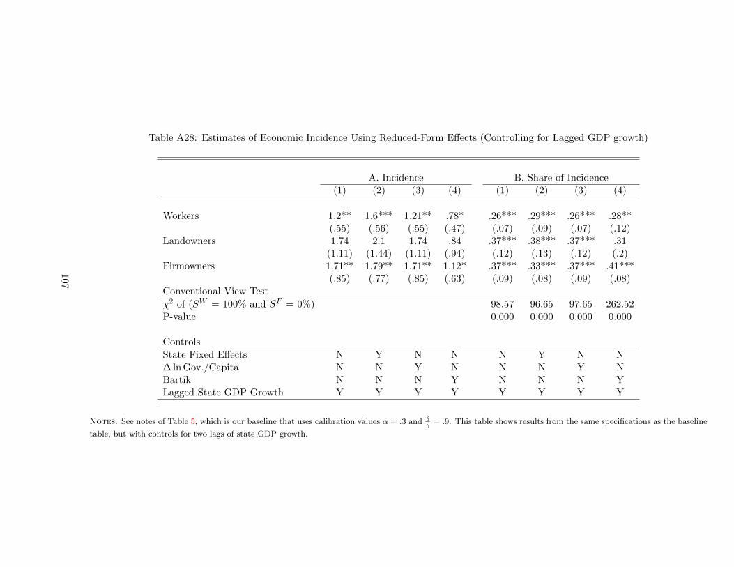
Table A28: Estimates of Economic Incidence Using Reduced-Form E↵ects (Controlling for Lagged GDP growth)

A. Incidence B. Share of Incidence(1) (2) (3) (4) (1) (2) (3) (4)

Workers 1.2** 1.6*** 1.21** .78* .26*** .29*** .26*** .28**(.55) (.56) (.55) (.47) (.07) (.09) (.07) (.12)

Landowners 1.74 2.1 1.74 .84 .37*** .38*** .37*** .31(1.11) (1.44) (1.11) (.94) (.12) (.13) (.12) (.2)

Firmowners 1.71** 1.79** 1.71** 1.12* .37*** .33*** .37*** .41***(.85) (.77) (.85) (.63) (.09) (.08) (.09) (.08)

Conventional View Test�2 of (SW = 100% and SF = 0%) 98.57 96.65 97.65 262.52P-value 0.000 0.000 0.000 0.000

ControlsState Fixed E↵ects N Y N N N Y N N� lnGov./Capita N N Y N N N Y NBartik N N N Y N N N YLagged State GDP Growth Y Y Y Y Y Y Y Y

Notes: See notes of Table 5, which is our baseline that uses calibration values ↵ = .3 and ��= .9. This table shows results from the same specifications as the baseline

table, but with controls for two lags of state GDP growth.

107

Table A29: Estimates of Economic Incidence Using Reduced-Form E↵ects (Dropping 1980-1990)

A. Incidence B. Share of Incidence(1) (2) (3) (4) (1) (2) (3) (4)

Workers 1.49** 2.15** 1.51** .99* .35** .72 .35** .33(.66) (.89) (.65) (.56) (.16) (.93) (.16) (.27)

Landowners .91 -.82 .93 .62 .21 -.28 .21 .21(1.66) (3.06) (1.65) (1.79) (.27) (1.43) (.27) (.42)

Firmowners 1.89* 1.64 1.9* 1.36 .44*** .55 .44*** .46***(.98) (1.16) (.97) (1.08) (.14) (.54) (.14) (.16)

Conventional View Test�2 of (SW = 100% and SF = 0%) 68.57 2.72 67.76 70.65P-value 0.000 0.100 0.000 0.000

ControlsState Fixed E↵ects N Y N N N Y N N� lnGov./Capita N N Y N N N Y NBartik N N N Y N N N Y

Notes: See notes of Table 5, which is our baseline that uses calibration values ↵ = .3 and ��= .9. This table shows results from the same specifications as the baseline

table, but without the 490 observations for the change from 1980-1990. There are 980 observations in each specification. We provide this table to address potential

concerns regarding the sensitivity of the results to the Tax Reform Act of 1986.

108

Table A30: Incidence Estimates Using Reduced-Form E↵ects with Tax Rate Controls

Panel (a) Incidence(1) (2) (3) (4)

Workers w � ↵r 1.1* 1.49** 1.1* 1.59**(.61) (.59) (.61) (.66)

Landowners r 1.07 1.15 1.21 1.2(1.48) (1.52) (1.25) (1.6)

Firmowners ⇡ 1.56* 1.69** 1.64* 1.75*(.91) (.76) (.88) (.9)

Panel (b) Shares of Incidence(1) (2) (3) (4)

Worker Share .29*** .34*** .28*** .35***(.11) (.13) (.09) (.12)

Landowner Share .29 .27 .31* .26(.21) (.22) (.16) (.23)

Firmowner Share .42*** .39*** .42*** .39***(.13) (.12) (.11) (.14)

Conventional View Test�2 of (SW = 100% and SF = 0%) 130.8 83.3 104 69.7

0.000 0.000 0.000 0.000Specifications

State Sales Tax Rate Y N N YState Individual Income Tax Rate N Y N YState Property Tax Rate N N Y Y

Notes: See notes of Table 5, which is our baseline that uses calibration values ↵ = .3 and ��= .9. This table shows

results from the same specifications as the baseline table, but with controls for di↵erent state tax rates. See Table A4

for notes on data sources.

109

Table A31: Incidence Estimates Using Reduced-Form E↵ects with Tax Rate Change Controls

Panel (a) Incidence(1) (2) (3) (4)

Workers w � ↵r 1.1* 1.08* 1.13*** 1.12***(.59) (.59) (.37) (.37)

Landowners r 1.15 1.21 1.24 1.3(1.43) (1.4) (1.15) (1.1)

Firmowners ⇡ 1.63* 1.65* 1.67** 1.72**(.9) (.93) (.69) (.73)

Panel (b) Shares of Incidence(1) (2) (3) (4)

Worker Share .28*** .27*** .28*** .27***(.09) (.09) (.09) (.08)

Landowner Share .3 .31* .31* .31**(.19) (.17) (.17) (.15)

Firmowner Share .42*** .42*** .41*** .41***(.12) (.11) (.11) (.09)

Conventional View Test�2 of (SW = 100% and SF = 0%) 137.7 141.6 139.8 154.7

0.000 0.000 0.000 0.000Specifications

� State Sales Tax Rate Y N N Y� State Income Tax Rate N Y N Y� State Property Tax Rate N N Y Y

Notes: See notes of Table 5, which is our baseline that uses calibration values ↵ = .3 and ��= .9. This table shows

results from the same specifications as the baseline table, but with controls for di↵erent state tax rates. See Table A4

for notes on data sources.

110

Table A32: Empirical and Predicted Moments from Structural Model

Panel (a) Business Tax ShockPopulation Wage Rent Establishments

Empirical MomentsBusiness Tax 4.275*** 1.451 1.172 4.074**

(1.642) (0.938) (1.428) (1.815)A. Predicted Moments (� = .15, "PD = �2.5)Business Tax 3.514 0.839 0.591 4.542

Over-id Test Test: �E = �N � (�("PD + 1)� 1)�W

�2-Stat 2.453 T-stat -1.566�2-P-Value 0.117 P-value 0.117

Panel (b) All ShocksPopulation Wage Rent Establishments

Empirical MomentsBusiness Tax 1.516 1.534 1.857 1.749

(1.915) (1.117) (1.562) (1.540)

Bartik 0.446** 0.554*** 0.697*** 0.600***(0.183) (0.079) (0.257) (0.189)

Personal Tax 1.731 -0.588 -1.192 1.247(1.247) (0.728) (1.173) (1.420)

B. Predicted Moments (� = .15, "PD = �2.5)Business Tax 0.736 0.944 1.111 1.893

Bartik 0.424 0.571 0.730 0.479

Personal Tax 1.052 -0.596 -1.559 0.322Over-id Test Test: �E = �N � (�("PD + 1)� 1)�W

�2-Stat 4.665 T-stat -1.217�2-P-Value 0.458 P-value 0.224

C. Predicted Moments (� = .15,↵ = .30) and estimated "PD

Business Tax 0.583 0.646 0.420 1.589

Bartik 0.397 0.572 0.725 0.447

Personal Tax 1.053 -0.359 -0.996 0.495Over-id Test Test: �E = �N � (�("PD + 1)� 1)�W

�2-Stat 5.378 T-stat -1.334�2-P-Value 0.251 P-value 0.182

Notes: This table shows the estimated reduced forms used in our minimum distance estimation as well as the models

predicted by our model. The reduced forms are estimated via a system OLS. The data are decade changes from

1980-1990, 1990-2000, and 2000-2010 for 490 county-groups. See Section 4 for data sources. All parameters assume

� = 0.9⇥ � and ↵ = 0.3. In addition, Panel (a) presents estimates of the model using only the tax shock for parameters

(� = .15, "PD = �2.5); panel (b) uses the business tax shock, the Bartik shock and the personal income tax shock

for parameters (� = .15, "PD = �2.5); and Panel (c) uses all shocks, calibrates � = .15 and estimates "PD. Results

of the �2 test of over identifying restrictions are below each model along with the result of the test of the restriction

�E = �N � (�("PD + 1) � 1)�W that is implied by calibrating "PD. See Section 6 for more details on the estimation.

Regressions use initial population as weights and include year fixed e↵ects and dummies for states in the industrial

midwest in the 1980s. Standard errors clustered by state are in parentheses and *** p<0.01, ** p<0.05, * p<0.1.

111

Table A33: Estimates of Structural Parameters

(1) (2) (3) (4) (5) (6)Worker Location Housing Supply Firm Location

OLS IV OLS IV OLS CMD

Idiosyncratic Location 2.312*** 0.717***Preference Dispersion �W (0.767) (0.277)

Elasticity of Housing 0.963*** 0.834*Supply ⌘ (0.208) (0.432)

Idiosyncratic Location 0.331* 0.097*Productivity Dispersion �F (0.174) (0.058)

Output Elasticity -0.316of Labor � (0.225)

N 1470 1470 1470 1470 1470 1470Instrument Bartik & Tax Bartik & TaxFirst Stage F-stat 46.718 15.32Calibrated Parameters:"PD -2.5 -2.5� 0.15�W 0.7⌘ 1.75

Notes: This table shows the estimated coe�cients of the parameters in our structural model. The data are decade

changes from 1980-1990, 1990-2000, and 2000-2010 for 490 county-groups. See Section 4 for data sources. Col (1)-(2)

estimate the parameter of worker preference dispersion �W , Col (3)-(4) the parameter of the housing supply equation

⌘, and Col (5)-(6) the parameters of the firm location equation � and �F . Col (1)-(5) are estimated via OLS or IV as

noted and the parameters are recovered via delta-method calculations. Col (6) is recovered using a classical minimum

distance approach. See Section 6 for more details on the specific equations and calibration choices. "PD denotes the

elasticity of product demand. Regressions use initial population as weights and include year fixed e↵ects and dummies

for states in the industrial midwest in the 1980s. Standard errors clustered by state are in parentheses and *** p<0.01,

** p<0.05, * p<0.1.

112

Table A34: Policy Probit of Payroll Apportionment Weight Changes

Independent Variables Coe�cient Standard ErrorMean Payroll Weight of Other States -.3608*** (.114)Mean Payroll Weight of Other States (t� 1) .2737 (.1947)Mean Payroll Weight of Other States (t� 2) .0491 (.1368)Corporate Tax Rate -.1225 (.2548)Corporate Tax Rate (t� 1) .2714 (.2813)Corporate Tax Rate (t� 2) -.128 (.1115)Individual Income Tax Rate .2006 (.2853)Individual Income Tax Rate (t� 1) -.4287 (.3978)Individual Income Tax Rate (t� 2) .2957 (.2492)State Income Growth (t� 1) -1.4585 (1.5766)State Income Growth (t� 2) -1.194 (1.5084)National Unemployment Rate (t� 1) -.0792 (.0776)National Unemployment Rate (t� 2) .0716 (.0938)

Notes: This table shows how observable economic and tax policy conditions relate to apportionment formula changes.

The specification is the same as the policy probit in Goolsbee and Maydew (2000). The dependent variable is an

indicator that equals one if payroll apportionment weights are changed. The analysis is at the state-year level for years

from 1978 through 2010. There are 1500 observations due to the lags. State income growth is the log di↵erence in per

capita GDP from BEA and the national unemployment rate is from BLS. Robust standard errors are in parentheses

and *** p<0.01, ** p<0.05, * p<0.1.

Table A35: Policy Probit of Statutory State Corporate Tax Changes

Independent Variables Coe�cient Standard ErrorMean Corporate Tax Rate of Other States 2.7234*** (.9537)Mean Corporate Tax Rate of Other States (t� 1) -3.9527*** (.9882)Mean Corporate Tax Rate of Other States (t� 2) .7191 (1.0997)Payroll Weight -.0227 (.0185)Payroll Weight (t� 1) .0056 (.0271)Payroll Weight (t� 2) .0312 (.0209)Individual Income Tax Rate -.2777 (.3036)Individual Income Tax Rate (t� 1) .1707 (.3773)Individual Income Tax Rate (t� 2) .0875 (.223)State Income Growth (t� 1) -.6771 (1.2064)State Income Growth (t� 2) .1552 (1.5484)National Unemployment Rate (t� 1) -.0539 (.089)National Unemployment Rate (t� 2) .0783 (.0779)

Notes: This table shows how observable economic and tax policy conditions relate to statutory state corporate tax

rate changes. The specification is the same as the policy probit in Goolsbee and Maydew (2000), but with a di↵erent

dependent variable. The dependent variable is an indicator that equals one if the statutory state corporate tax rate

change exceeds 0.5 percentage points. The analysis is at the state-year level for years from 1978 through 2010. There

are 1500 observations due to the lags. State income growth is the log di↵erence in per capita GDP from BEA and

the national unemployment rate is from BLS. Robust standard errors are in parentheses and *** p<0.01, ** p<0.05, *

p<0.1.

113

Table A36: Revenue-Maximizing Corporate Tax Rates By StateEstablishment Revenue Ratio Sales Apport. Corporate Revenue Max. Corp. Rate

State Share Es revperss /revC

s Weight ✓xs Tax Rate ⌧s ⌧⇤s ⌧⇤⇤

s ⌧⇤⇤s /(1� ✓xs )

Alabama 1.4 16.4 33 6.5 30.6 2.2 3.3Alaska 0.3 0.4 33 9.4 32.3 24.1 36.1Arizona 1.8 22.1 80 7.0 30.0 1.7 8.3Arkansas 0.9 15.0 50 6.5 30.7 2.4 4.7California 11.7 9.2 50 8.8 32.0 3.7 7.4Colorado 2.1 21.1 100 4.6 31.0 1.7Connecticut 1.2 21.9 50 7.5 31.0 1.7 3.3Delaware 0.3 9.2 33 8.7 29.6 3.7 5.5Florida 6.7 14.6 50 5.5 31.2 2.4 4.9Georgia 3.0 19.8 100 6.0 29.6 1.8Hawaii 0.4 57.3 33 6.4 28.6 0.7 1.0Idaho 0.6 26.2 50 7.6 33.8 1.4 2.8Illinois 4.3 9.0 100 7.3 31.6 3.8Indiana 2.0 20.7 90 8.5 32.9 1.8 17.7Iowa 1.1 30.4 100 12.0 32.0 1.2Kansas 1.0 16.0 33 7.1 30.6 2.2 3.4Kentucky 1.2 20.4 50 6.0 31.3 1.8 3.6Louisiana 1.4 18.1 100 8.0 32.2 2.0Maine 0.6 16.9 100 8.9 34.0 2.1Maryland 1.8 14.0 50 8.3 31.6 2.5 5.1Massachusetts 2.3 9.2 50 8.8 31.9 3.7 7.4Michigan 3.0 26.4 100 4.9 31.5 1.4Minnesota 2.0 19.9 87 9.8 33.2 1.8 14.1Mississippi 0.8 17.2 33 5.0 30.5 2.1 3.1Missouri 2.1 42.8 33 6.3 31.2 0.9 1.3Montana 0.5 13.4 33 6.8 36.8 2.7 4.0Nebraska 0.7 22.1 100 7.8 31.6 1.7Nevada 0.8 100 0.0 29.2New Hampshire 0.5 2.0 50 8.5 31.2 12.1 24.1New Jersey 3.1 10.6 50 9.0 31.0 3.3 6.5New Mexico 0.6 26.1 33 7.6 32.0 1.4 2.1New York 7.1 14.3 100 7.1 34.6 2.5North Carolina 3.0 14.3 50 6.9 31.3 2.5 5.0North Dakota 0.3 14.2 33 6.4 35.3 2.5 3.8Ohio 3.5 141.5 60 8.5 31.4 0.3 0.7Oklahoma 1.2 24.0 33 6.0 31.7 1.5 2.3Oregon 1.5 16.8 100 7.9 32.8 2.1Pennsylvania 4.1 15.1 90 10.0 33.2 2.4 23.9Rhode Island 0.4 19.0 33 9.0 34.5 1.9 2.9South Carolina 1.4 45.1 100 5.0 30.6 0.8South Dakota 0.4 34.7 100 0.0 36.5 1.1Tennessee 1.8 9.1 50 6.5 29.4 3.7 7.4Texas 7.2 100 0.0 30.3Utah 0.9 18.3 50 5.0 31.4 2.0 4.0Vermont 0.3 15.7 50 8.5 34.7 2.3 4.6Virginia 1.5 18.4 50 6.0 30.1 2.0 3.9Washington 2.4 100 0.0 31.9West Virginia 0.5 16.3 50 8.5 30.8 2.2 4.4Wisconsin 1.9 14.7 100 7.9 32.8 2.4

Notes: This table shows the corporate tax revenue-maximizing corporate tax rate ⌧⇤s and the total tax revenue-

maximizing corporate tax rate ⌧⇤⇤s , which accounts for some fiscal externalities. These calculations are based on 2010

data and average national parameter estimates and do not incorporate heterogeneous housing markets. SeeSection 7 and Section D in the appendix for details. Sources: U.S. Census ASG and those in Section 4.

114

Figure A1: Time Series of State Corporate Tax Rates by State

115

Figure A2: State Corporate Tax Apportionment Rules in 2012

A. Payroll Apportionment Rate by State

25.00 − 33.3322.50 − 25.000.00 − 22.500.00 − 0.00

B. Sales Apportionment Rate by State

55.0 − 100.033.3 − 50.033.3 − 33.3

116

Figure A3: 30 Year Change State Corporate Tax Rates and Rules: 1980-2010

A. Corporate Tax Rate Changes by State

2.00 − 5.501.00 − 2.000.35 − 1.000.00 − 0.35-0.51 − 0.00-3.03 − -0.51

B. Sales Apportionment Rate Changes by State

16.66 − 66.660.00 − 16.660.00 − 0.00

117

Figure A4: Shares of Total U.S. Establishments and Population in 2010

A. Establishment Share by State

2.96 − 11.491.96 − 2.961.34 − 1.960.80 − 1.340.43 − 0.800.27 − 0.43

B. Population Share by State

1.68 − 6.381.12 − 1.680.76 − 1.120.48 − 0.760.26 − 0.480.12 − 0.26

118

Figure A5: 30 Year Change in Share of Establishments and Population: 1980-2010

A. Change in Establishment Share by State

21.51 − 68.676.82 − 21.51-4.76 − 6.82-11.43 − -4.76-18.42 − -11.43-29.87 − -18.42

B. Change in Population Share by State

29.76 − 80.2117.09 − 29.766.17 − 17.091.39 − 6.17-6.20 − 1.39-16.02 − -6.20

119

Figure A6: Decadal Changes in State Corporate Tax Policy

Panel (a) Corporate Tax Rate Changes

050

100

150

Freq

uenc

y

-.04 -.02 0 .02 .04 .06Ten Year Change in Statutory State Corporate Tax Rate

Panel (b) Payroll Apportionment Weight Changes

050

100

150

200

250

Freq

uenc

y

-.3 -.2 -.1 0Ten Year Change in Payroll Apportionment Weight

Notes: These figures show changes in corporate tax policy in the baseline PUMA-decade sample of 490 PUMAs over

1980-1990, 1990-2000, and 2000-2010. Panel (a) is a histogram showing the distribution of non-zero changes in corporate

tax rates in the pooled sample. Panel (b) is a similar figure for payroll apportionment weights.

120

Figure A7: Testing for Concomitant Tax Base Changes

−3

−2

−1

01

2C

ha

ng

e in

Sta

te C

orp

ora

te R

ate

0 2 4 6 8 10Change in State ITC

95% CI Linear Fit Binned Data

Data from Wilson and Chirinko (2008). 10 Yr Changes. D.Corp= 0.2 + 0.026 (D.ITC), with se=.06

Notes: This figure, which uses data generously provided by Chirinko and Wilson (2008), illustrates that there is no

detectable relationship between corporate tax rate changes and investment tax credit changes. It shows the average

state corporate tax rate change for di↵erent bins of state investment credit changes. The estimated relationship is

�⌧ cs,t = 0.2 + 0.026�ITCs,t, with se=0.06 and R2 = .001. Changes are measured over ten-year periods.

121

Figure A8: Cumulative E↵ects of Business Tax Cuts on Population Growth

-50

510

15Pe

rcen

t

-10 -5 0 5 10Year

Cumulative Effect no leads Cumulative Effect w/ leadsLong Difference Point Estimate 95 % Confidence Interval

Notes: This figure shows the cumulative annual e↵ects of local business tax cuts on local population growth over

di↵erent time horizons with pre-trends. It plots the analogous estimates as Figure 4. See Section 4 for data sources and

Section E for estimation details.

122

Figure A9: Cumulative E↵ects of Business Tax Cuts on Growth in Gross Operating Surplus

F-test all leads are 0 has p-value= 0.84 F-test all lags are 0 has p-value= 0.0005

-10

-50

510

Perc

ent

-10 -5 0 5 10Year

Cumulative Effect no leads Cumulative Effect w/ leadsLong Difference Point Estimate 95 % Confidence Interval

Notes: This figure shows the cumulative annual e↵ects of local business tax cuts on state gross operating surplus over

di↵erent time horizons with pre-trends. It plots the analogous estimates as Figure 4. See Section 4 for data sources and

Section E for estimation details.

123

Figure A10: E↵ect of Business Tax Cut on Establishment Growth over 10 Years

.1.1

5.2

.25

10 Y

ear L

og C

hang

e in

Est

ablis

hmen

ts

-.02 -.015 -.01 -.005 0 .005 10 Year Log Change in Net of Business Tax Rate

Slope= 3.94 (1.61)

Notes: This figure shows the mean log change in the number of establishments over 10 years by bin of log change in

the net-of-business-tax rate ⌧ b over 10 years. The data are unweighted, at the county-group level, and are only adjusted

for year fixed e↵ects. Standard errors clustered by state are in parentheses and *** p<0.01, ** p<0.05, * p<0.1.

124

Figure A11: E↵ect of Business Tax Cut on Population Growth over 10 Years

.05

.1.1

5.2

10 Y

ear L

og C

hang

e in

Pop

ulat

ion

-.02 -.015 -.01 -.005 0 .005 10 Year Log Change in Net of Business Tax Rate

Slope= 3.94 (1.57)

Notes: This figure shows the mean log change in the population over 10 years by bin of log change in the net-of-

business-tax rate ⌧ b over 10 years. The data are unweighted, at the county-group level, and are only adjusted for year

fixed e↵ects. Standard errors clustered by state are in parentheses and *** p<0.01, ** p<0.05, * p<0.1.

125

Figure A12: E↵ect of Business Tax Cut on Wage Growth over 10 Years

-.1-.0

50

.05

10 Y

ear L

og C

hang

e in

Com

posi

tion

Adj.

Wag

es

-.02 -.015 -.01 -.005 0 .005 10 Year Log Change in Net of Business Tax Rate

Slope= 1.78 (.72)

Notes: This figure shows the mean log change in wages over 10 years by bin of log change in the net-of-business-tax

rate ⌧ b over 10 years. The data are unweighted, at the county-group level, and are only adjusted for year fixed e↵ects.

As in the main text, wages are a composition constant index. Standard errors clustered by state are in parentheses and

*** p<0.01, ** p<0.05, * p<0.1.

126

Figure A13: E↵ect of Business Tax Cut on Rental Cost Growth over 10 Years

-.05

0.0

5.1

.15

10 Y

ear L

og C

hang

e in

Com

posi

tion

Adj R

ents

-.02 -.015 -.01 -.005 0 .005 10 Year Log Change in Net of Business Tax Rate

Slope= 2.16 (1.4)

Notes: This figure shows the mean log change in rents over 10 years by bin of log change in the net-of-business-tax rate

⌧ b over 10 years. The data are unweighted, at the county-group level, and are only adjusted for year fixed e↵ects. As

in the main text, rental costs are a composition constant index. Standard errors clustered by state are in parentheses

and *** p<0.01, ** p<0.05, * p<0.1.

127

Figure A14: E↵ect of Business Tax Cut on Growth in GOS per Establishment over 10 Years

.35

.4.4

5.5

.55

10 Y

ear L

og C

hang

e in

GO

S pe

r Est

ablis

hmen

t

-.02 -.015 -.01 -.005 0 .00510 Year Log Change in Net of Business Tax Rate

Slope= 3.53 (1.76)

Notes: This figure shows the mean log change in state gross operating surplus per establishment over 10 years by bin

of log change in the net-of-business-tax rate ⌧ b over 10 years. The data are unweighted, at the county-group level, and

are only adjust for year fixed e↵ects. To account for the consumption of fixed capital, which is 44% of GOS on average

during the sample period of 1980 to 2010 (NIPA Table 1.14), one needs to multiply this point estimate by (1-.44).

In particular, the point estimate implies an estimated e↵ect of (1 � .44) ⇥ 3.53 = 1.98 on net operating surplus per

establishment. Standard errors clustered by state are in parentheses and *** p<0.01, ** p<0.05, * p<0.1.

128

Figure A15: E↵ect of Business Tax Cut on Growth in Sales Tax Revenue per Establishment

.3.4

.5.6

10 Y

r Log

Chg

in S

ales

Tax

Rev

per

Est

ablis

hmen

t

-.02 -.015 -.01 -.005 0 .00510 Year Log Change in Net of Business Tax Rate

Slope= 2.12 (3.04)

Notes: This figure shows the mean log change in state sales tax revenue per establishment over 10 years by bin of log

change in the net-of-business-tax rate ⌧ b over 10 years. The data are unweighted, at the county-group level, and are

only adjust for year fixed e↵ects. Standard errors clustered by state are in parentheses and *** p<0.01, ** p<0.05, *

p<0.1.

129

Figure A16: Estimates of Worker Location Equation

σIVW = 0.72** (0.28)

σOLSW = 2.31*** (0.77)

-.1-.0

50

.05

.1Lo

g Ch

ange

in P

opul

atio

n

-.1 -.05 0 .05 .1Log Change in Real Wage

Binned Pop Growth Binned FS Fit of Pop GrowthOLS IV

Notes: This figure illustrates the importance of accounting for regional amenities when estimating the parameters

that govern worker mobility. Ignoring amenity changes attenuates the e↵ects of wage changes on population changes.

In particular, the figure shows the mean log change in population by bin of log change in real wage as well as the

fitted values of a first stage regression of real wage on the Bartik shock and the tax shock. Using these fitted values

illustrates how real wage changes (that are orthogonal to amenity changes) relate to population changes. The fitted

lines in the figure plot the associated estimates via OLS and IV from Table A33. Standard errors clustered by state are

in parentheses and *** p<0.01, ** p<0.05, * p<0.1.

130

Figure A17: Estimates of Establishment Location Equation

σCMDF = 0.1** (0.06)

σOLSF = 0.331*** (0.17)

-.1-.0

50

.05

.1Lo

g Ch

ange

in E

stab

lishm

ents

-.02 -.01 0 .01 .02Log Change in Net of Bus Tax

Binned Est Growth OLSCMD Conventional Wisdom

Notes: This figure illustrates how establishment location choices relate to business taxes. The conventional view on

corporate taxation in an open economy, which is based on models that neither incorporate the location decisions of

business nor the possibility that a business’s productivity can di↵er across locations, e↵ectively implies that business

location will be very responsive to tax di↵erentials over the long-run (Gordon and Hines, 2002). This figure shows how

this conventional wisdom on responsiveness compares to the empirical responsiveness of location decisions to business

tax changes over a ten-year period. In particular, it shows the mean log change in establishments by bin of log change

in the net-of-business-tax rate. The fitted lines plot the associated estimates via OLS and classical minimum distance

(CMD) from Table A33 Col. 5 and 6, respectively (see Section E.6.4 for more detail). The OLS line shows the

relationship between log changes in net-of-business-taxes and establishment growth. The positive slope indicates that

tax cuts increase the number of local establishments over a ten-year period. However, ignoring equilibrium e↵ects of

tax changes on wages attenuates the e↵ects of business tax changes on establishment growth. The CMD line shows

that accounting for these impacts increases estimated responsiveness. Nonetheless, accounting for equilibrium impacts

still yields substantially lower responsiveness to tax changes than the conventional wisdom implies. Section 2 quantifies

how lower responsiveness a↵ects the incidence and e�ciency of corporate taxation. Standard errors clustered by state

are in parentheses and *** p<0.01, ** p<0.05, * p<0.1. See Appendix Figure A16 for the analogous figure for worker

location.

131

Figure A18: Robustness of Economic Incidence

Panel (a)Landowner’s Share of Incidence for ↵ = 0.3 and Calibrated Values of � and "PD

* Baseline-5

-4-3

-2El

astic

ity o

f Pro

duct

Dem

and:

εPD

0 .1 .2 .3 .4 .5Output Elasticity of Labor: γ

.3

.4

.5

.6

.7

.8

.9

Shar

e to

Lan

d O

wner

s

Panel (b)Landowner’s Share of Incidence for � = .15 and Calibrated Values of ↵ and "PD

* Baseline

-5-4

-3-2

Elas

ticity

of P

rodu

ct D

eman

d: εP

D

0 .2 .4 .6 .8 1Housing Expenditure Share: α

.3

.4

.5

.6

.7

.8

.9

Shar

e to

Lan

d O

wner

s

Notes: This figure, which is analogous to Figure 5 for landowners instead of firm owners, shows how our estimates

of landowner incidence vary across the parameter space. Specifically, the figures plot landowner incidence shares for

a variety of parameter values relative to our baseline parameters values of � = 0.15, "PD = �2.5, and ↵ = .3. See

Section 6 for more detail.

132

Figure A19: Robustness of Economic Incidence

Panel (a)Workers’ Share of Incidence for ↵ = 0.3 and Calibrated Values of � and "PD

* Baseline-5

-4-3

-2El

astic

ity o

f Pro

duct

Dem

and:

εPD

0 .1 .2 .3 .4 .5Output Elasticity of Labor: γ

.3

.4

.5

.6

.7

.8

.9

Shar

e to

Wor

kers

Panel (b)Workers’ Share of Incidence for � = .15 and Calibrated Values of ↵ and "PD

* Baseline

-5-4

-3-2

Elas

ticity

of P

rodu

ct D

eman

d: εP

D

0 .2 .4 .6 .8 1Housing Expenditure Share: α

.3

.4

.5

.6

.7

.8

.9

Shar

e to

Wor

kers

Notes: This figure, which is analogous to Figure 5 for workers instead of firm owners, shows how our estimates of

worker incidence vary across the parameter space. Specifically, the figures plot worker incidence shares for a variety of

parameter values relative to our baseline parameters values of � = 0.15, "PD = �2.5, and ↵ = .3. See Section 6 for

more detail.

133

Figure A20: Robustness of Economic Incidence (Using Employment E↵ects)

Panel (a)Firm Owner’s Share of Incidence for ↵ = 0.3 and Calibrated Values of � and "PD

* Baseline-5

-4-3

-2El

astic

ity o

f Pro

duct

Dem

and:

εPD

0 .1 .2 .3 .4 .5Output Elasticity of Labor: γ

.3

.4

.5

.6

.7

.8

.9

Shar

e to

Firm

Own

ers

Panel (b)Firm Owner’s Share of Incidence for � = .15 and Calibrated Values of ↵ and "PD

* Baseline

-5-4

-3-2

Elas

ticity

of P

rodu

ct D

eman

d: εP

D

0 .2 .4 .6 .8 1Housing Expenditure Share: α

.2

.3

.4

.5

.6

.7Sh

are

to F

irm O

wner

s

Notes: This figure, which is analogous to Figure 5 for firm owners based on employment changes rather than based

on population changes (i.e., using the estimates in Table A9 instead of A6), shows how our estimates of firm owner

incidence vary across the parameter space. Specifically, the figures plot firm owner incidence shares for a variety of

parameter values relative to our baseline parameters values of � = 0.15, "PD = �2.5, and ↵ = .3. See Section 6 for

more detail.

134

Figure A21: Robustness of Economic Incidence

Share of Incidence for Calibrated Values of � and Estimated "PD

020

4060

80Sh

are

of In

ciden

ce

0 .1 .2 .3 .4 .5Output Elasticity of Labor: γ

Firms Workers Land

Notes: This figure shows that the shares of incidence to firm owners, workers, and landowners are independent of

the calibrated values for the output elasticity of labor �. Similar to Part A of Figure 5, it indicates that our baseline

empirical result – that firm owners bear a substantial share of incidence – is robust to using a variety of calibrated

parameter values. Appendix Figure A22 shows the relationship between calibration values and estimates as well as their

implications for markups. See Section 3 for more detail.

135

Figure A22: Estimates of "PD and Associated Markups for Values of �

Panel (a) Estimates of "PD

-5-4

.5-4

-3.5

Elas

ticity

of P

rodu

ct D

eman

d: εP

D

0 .1 .2 .3 .4 .5Output Elasticity of Labor: γ

Panel (b) Estimates of Product Markups

2530

35M

arku

p (%

)

-5 -4.5 -4 -3.5Elasticity of Product Demand: εPD

Notes: These figures show the estimated value of "PD for di↵erent values of � in Panel (a). These estimates correspond

to di↵erent version of the CMD model with two shocks as in Panel (b) of Table 6. Panel (b) plots the associated markup

for a given value of "PD.

136