Who Dominates the U.S. Soybean Industry: Producers ...ageconsearch.umn.edu/bitstream/20117/1/sp04so02.pdf · Who Dominates the U.S. Soybean Industry: Producers, Consumers, or Agribusinesses?

Who Dominates the U.S. Soybean Industry: Producers, Consumers, or Agribusinesses?

Baohui Song Research Assistant University of Kentucky Department of Agricultural Economics 417 C. E. Barnhart Bldg. Lexington, KY 40546-0276 Phone: (859) 257-7283 Fax: (859) 257-7290 E-mail: [email protected] Shuang Xu Research Assistant University of Kentucky Department of Agricultural Economics 417 C. E. Barnhart Bldg. Lexington, KY 40546-0276 Phone: (859) 257-7283 Fax: (859) 257-7290 E-mail: [email protected]

Mary A. Marchant Professor University of Kentucky Department of Agricultural Economics 314 C. E. Barnhart Bldg. Lexington, KY 40546-0276 Phone: (859) 257-7260 Fax: (859) 257-7290 E-mail: [email protected]

Selected Paper prepared for presentation at the American Agricultural Economics Association

Annual Meeting, Denver, Colorado, August 1-4, 2004

Copyright 2004 by Baohui Song, Mary A. Marchant, and Shuang Xu. All rights reserved. Readers may make verbatim copies of this document for non-commercial purposes by any means, provided that this copyright notice appears on all such copies.

PDF created with pdfFactory trial version www.pdffactory.com

mailto:[email protected]



http://www.pdffactory.com

1


Abstract

Globally the U.S. is the number one producer, consumer and exporter of soybeans.

Nationally, U.S. soybean production value ranks second among all agricultural bulk

commodities, having a significant impact on U.S. farm incomes. U.S. soybean has been a

subsidized commodity since 1941 and the 2002 Farm Bill provides soybeans for the first time

direct government payment and counter-cyclical payments. Using welfare economics, this

research explores the political economy of U.S. soybean subsidy policies. Results for the U.S.

soybean industry indicate that in aggregate terms, consumer interests dominate and in per capita

terms, producer interests dominate.

Introduction

An Overview of U.S. Soybeans

The soybean industry in the U.S. plays an important role in the world. Globally, the U.S.

is the leading country in soybean production, consumption and exports as shown in figure 1-a,

figure 1-b, and figure 1-c. These three figures also show that in the last decade, Brazil and

Argentina have become major competitors for the U.S. in the world soybean market (Schnefp,

Dohlman, and Bolling, 2001). In 2003, U.S. soybean production was 65.80 million metric tons,

accounting for 35% of world production; U.S. soybean consumption was 43.25 million metric

tons, 21.68% of world consumption; and U.S. soybean exports were 24.49 million metric tons,

39.07% of world exports (FAO, 2004). However, U.S. soybean imports were very low, only 0.22

million metric tons in 2003 (USDA-FAS, 2004).



2

Figure 1-a. Soybean Production Comparison between the U.S. and other Countries. Source: FAO, online statistical databases, 2004.

Figure 1-b. Soybean Consumption Comparison between the U.S. and Other Countries. Source: USDA-FAS, PS&D online dataset, 2004.

65.80

51.55

34.80

16.50

20.88

0

50

100

150

200

1964 1967 1970 1973 1976 1979 1982 1985 1988 1991 1994 1997 2000 2003

(Mill

ion

Met

ric T

ons)

s

the U.S. Brazil Argentina China Others

57.62

43.25

37.89

34.95

25.80

0

50

100

150

200

1964 1967 1970 1973 1976 1979 1982 1985 1988 1991 1994 1997 2000 2003

(Mill

ion

Met

ric T

ons)

.

Others the U.S. China Brazil Argentina



3

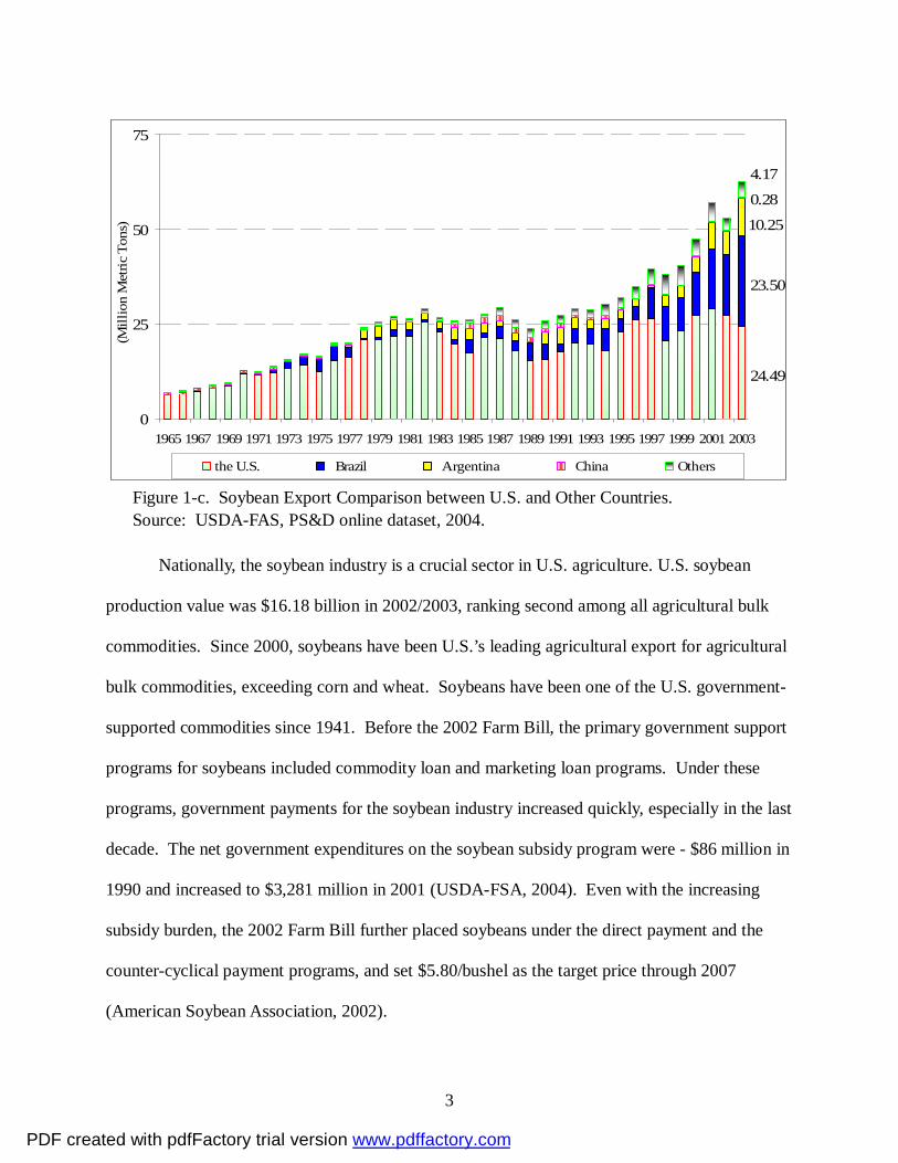
Figure 1-c. Soybean Export Comparison between U.S. and Other Countries. Source: USDA-FAS, PS&D online dataset, 2004.

Nationally, the soybean industry is a crucial sector in U.S. agriculture. U.S. soybean

production value was $16.18 billion in 2002/2003, ranking second among all agricultural bulk

commodities. Since 2000, soybeans have been U.S.’s leading agricultural export for agricultural

bulk commodities, exceeding corn and wheat. Soybeans have been one of the U.S. government-

supported commodities since 1941. Before the 2002 Farm Bill, the primary government support

programs for soybeans included commodity loan and marketing loan programs. Under these

programs, government payments for the soybean industry increased quickly, especially in the last

decade. The net government expenditures on the soybean subsidy program were - $86 million in

1990 and increased to $3,281 million in 2001 (USDA-FSA, 2004). Even with the increasing

subsidy burden, the 2002 Farm Bill further placed soybeans under the direct payment and the

counter-cyclical payment programs, and set $5.80/bushel as the target price through 2007

(American Soybean Association, 2002).

24.49

23.50

10.25

0.28

4.17

0

25

50

75

1965 1967 1969 1971 1973 1975 1977 1979 1981 1983 1985 1987 1989 1991 1993 1995 1997 1999 2001 2003

(Mill

ion

Met

ric T

ons)

s




4

Objectives

In this research, our objectives include 1) developing a soybean model at the industry

level, which incorporates endogenous supply, demand and prices and other related exogenous

variables; 2) estimating the model as a simultaneous equation system; 3) conducting economics

welfare analyses for the U.S. soybean industry; 4) identifying which interest group dominates the

U.S. soybean industry.

U.S. Government Soybean Subsidy Programs

The main U.S. soybean subsidy programs include soybean loan program and government

payments. The soybean loan program was first introduced in 1941 and has been in place since

then, except in 1975 (Westcott and Price, 2001). The original form of the soybean loan program

was the commodity loan program, which supported the market price. The marketing loan

program started in the mid-1980s, which mainly supported producers’ income instead of the

market prices.

Under the commodity loan program, producers must keep the crop designated as loan

collateral in approved storage to preserve the crop’s quality. Producers may choose to either

default on the loan at the end of the loan period, keeping the loan money and forfeiting

ownership of collateral to the government or sell the commodity and repay the loan plus interest,

depending on the market price level (Westcott and Price, 1999). While under the marketing loan

program producers may operate as described above. Alternatively, the marketing loan provisions

also allow repayment of commodity loans at less than the original loan rate when market prices

are lower (USDA-ERS, 2004). This feature decreases the loan program’s potential effect on

supporting prices because stock accumulation by the government, through loan defaults, is

reduced. Instead, farmers are provided economic incentives to retain ownership of the crops and



5

sell them rather than default on loans and forfeit ownership of the crops to the government

(Westcott and Price, 1999).

Another subsidy form for soybeans is government payments, including direct payments

and counter-cyclical payments within the 2002 Farm Bill. The formula for direct payments is:

Direct Payment = Base Acres x Program Yield x 85% x Direct Payment Rate

Base acres and program yields are calculated on the average level of the recent history of

planted acres and yields, while the direct payment rate (DPR) is decided by the USDA. The

2002 Farm Bill set the DPR for soybeans at $0.44/bushel. Direct payments only relate to the

planted area, so farmers and eligible landowners will receive annual direct payments.

The Counter-Cyclical Payments formula is:

Counter-Cyclical Payment=Base Acres × Program Yield × 85% × CCP Rate CCP Rate = Max (0, Target Price – Effective Price) Effective Price = Max (MYA Price, Loan Rate) + Direct Payment Rate

The MYA price is the marketing year average price, and the 2002 Farm Bill set the target

price for soybeans at $5.80/bushel. The counter-cyclical payment is closely related to the market

price. If the market price is high enough, the counter-cyclical payment will not occur.

Literature Review

In modeling the soybean industry, different methods have been employed. Piggott et al.

(2000), estimated soybeans, soybean meal and soybean oil demand and supply elasticities using

1974 to 1998 annual data. The cross effect between supply and demand could not be examined

because they estimated the demand and supply independently. Since they used the domestic

disappearance as the total demand, the effects of some exogenous factors on soybean supply and

demand cannot be examined. The USDA also has its own estimation model to predict the supply

and demand (Reed, et al., 2002). Given the estimated elasticities and baseline demand and prices,



6

they estimate the demand using a system of equations, including export demand, feed demand,

crushing demand, industrial demand, domestic demand, food demand, etc. Similar methods

were used for the supply side. Gardner (1990) used cross elasticities (among wheat, corn and

soybeans), estimated by Tyers and Anderson and Johnson et al., to determine producers’ gains

and losses. However, many previous works did not incorporate exports as an endogenous

variable in the model. The U.S. is the biggest soybean exporter in the world, and in 2003 U.S.

soybean exports comprised 37% of U.S. soybean output (USDA-FAS, 2004). The empirical

estimation results might not be reliable when the export effect on the U.S. soybean industry was

ignored. Modeling the Soybeans Industry

The Structure of the U.S. Soybean Industry

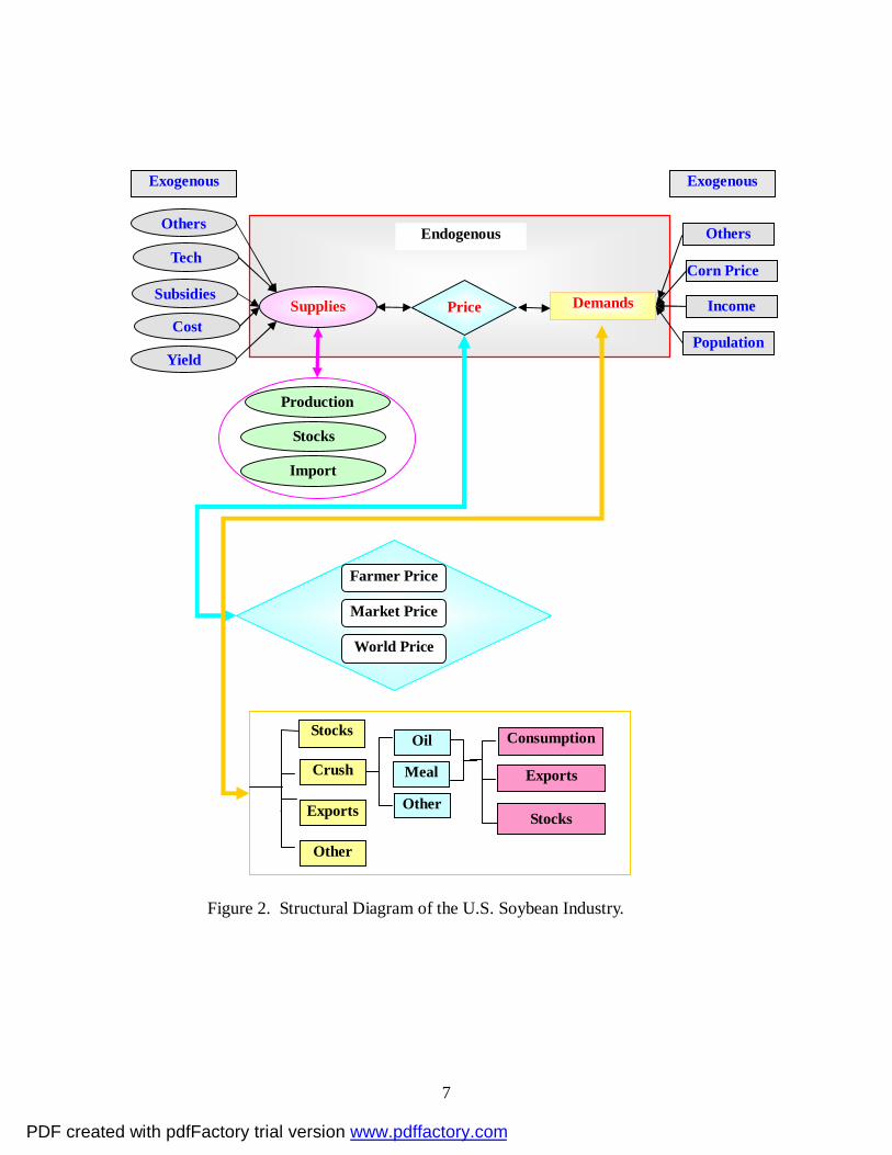
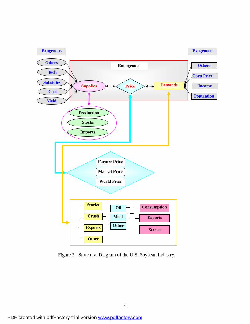
To accurately describe the U.S. soybean industry, the structure of the demand and supply

system and the factors that will affect the system were introduced first. As shown in Figure 3,

the entire soybean industry can be viewed as interaction of four components: supply, demand,

prices and exogenous factors.

Supply comes from three sources: production, beginning stocks and imports. Demand

includes four parts: crush demand, export demand, stocks, and others, among them the crushed

soybeans can be further divided into the sub-categories of soybean oil and soybean meal.

Soybean oil and soybean meal can be allocated based on usage into domestic consumption,

exports, and stocks. Three levels of soybean price---farm-level prices, retail-level prices and

world prices are taken into consideration as price variables. Seven defined exogenous variables

are included in this system. Technology, production cost, government subsidy and yield affect

the producer’s decision on outputs. Corn price (hypothesizing that corn is a substitute product

for soybeans), disposable personal income and population affect the total demand.



7

Production

Stocks

Import

Farmer Price

Market Price

Figure 2. Structural Diagram of the U.S. Soybean Industry.

World Price

Consumption

Exports Crush

Exports

Other

Oil

Meal

Other Stocks

Stocks

Exogenous

Population

Income Subsidies

Others

Cost

Yield

Supplies Demands Price

Exogenous

Corn Price

Others Tech

Endogenous



8

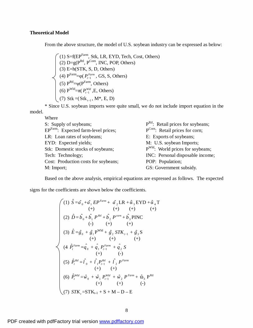
Theoretical Model

From the above structure, the model of U.S. soybean industry can be expressed as below:

(1) S=f(EPFarm, Stk, LR, EYD, Tech, Cost, Others) (2) D=g(PRtl, PCorn, INC, POP, Others) (3) E=h(STK, S, D, Others) (4) PFarm=φ( Farm

tP 1− , GS, S, Others) (5) PRtl=ψ(PFarm, Others) (6) PWld=π( Wld

tP 1− ,E, Others) (7) Stk =( 1tStk − , M*, E, D)

* Since U.S. soybean imports were quite small, we do not include import equation in the model.

Where S: Supply of soybeans; EPFarm: Expected farm-level prices; LR: Loan rates of soybeans; EYD: Expected yields; Stk: Domestic stocks of soybeans; Tech: Technology; Cost: Production costs for soybeans; M: Import;

PRtl: Retail prices for soybeans; PCorn: Retail prices for corn; E: Exports of soybeans; M: U.S. soybean Imports; PWld: World prices for soybeans; INC: Personal disposable income; POP: Population; GS: Government subsidy.

Based on the above analysis, empirical equations are expressed as follows. The expected

signs for the coefficients are shown below the coefficients.

(1) S = 0α + 1α FarmEP + 2α LR + 3α EYD + 4α T (+) (+) (+) (+)

(2) D = 0β + 1β RtlP + 2β cornP + 3β PINC (-) (+) (+)

(3) E = 0γ + 1γ PWld + 2γ 1−tSTK + 3γ S (+) (+) (+)

(4 FarmtP = 0θ + 1θ Farm

tP 1− + 2θ S (+) (-)

(5) RtltP = 0λ + Rtl

tP 11 −λ + 2λ FarmP (+) (+)

(6) WldtP = 0ω + 1ω Wld

tP 1− + 2ω FarmP + 3ω RtlP (+) (+) (-)

(7) tSTK =STKt-1 + S + M – D – E



9

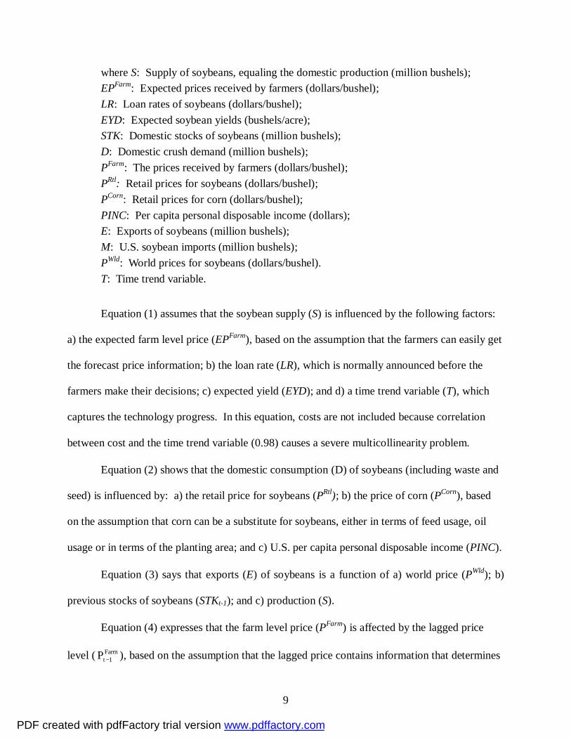
where S: Supply of soybeans, equaling the domestic production (million bushels); EPFarm: Expected prices received by farmers (dollars/bushel); LR: Loan rates of soybeans (dollars/bushel); EYD: Expected soybean yields (bushels/acre); STK: Domestic stocks of soybeans (million bushels); D: Domestic crush demand (million bushels); PFarm: The prices received by farmers (dollars/bushel); PRtl: Retail prices for soybeans (dollars/bushel); PCorn: Retail prices for corn (dollars/bushel); PINC: Per capita personal disposable income (dollars); E: Exports of soybeans (million bushels); M: U.S. soybean imports (million bushels); PWld: World prices for soybeans (dollars/bushel). T: Time trend variable. Equation (1) assumes that the soybean supply (S) is influenced by the following factors:

a) the expected farm level price (EPFarm), based on the assumption that the farmers can easily get

the forecast price information; b) the loan rate (LR), which is normally announced before the

farmers make their decisions; c) expected yield (EYD); and d) a time trend variable (T), which

captures the technology progress. In this equation, costs are not included because correlation

between cost and the time trend variable (0.98) causes a severe multicollinearity problem.

Equation (2) shows that the domestic consumption (D) of soybeans (including waste and

seed) is influenced by: a) the retail price for soybeans (PRtl); b) the price of corn (PCorn), based

on the assumption that corn can be a substitute for soybeans, either in terms of feed usage, oil

usage or in terms of the planting area; and c) U.S. per capita personal disposable income (PINC).

Equation (3) says that exports (E) of soybeans is a function of a) world price (PWld); b)

previous stocks of soybeans (STKt-1); and c) production (S).

Equation (4) expresses that the farm level price (PFarm) is affected by the lagged price

level ( Farm1tP − ), based on the assumption that the lagged price contains information that determines



10

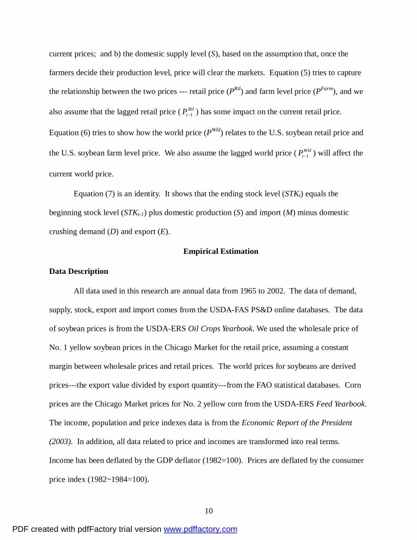
current prices; and b) the domestic supply level (S), based on the assumption that, once the

farmers decide their production level, price will clear the markets. Equation (5) tries to capture

the relationship between the two prices --- retail price (PRtl) and farm level price (PFarm), and we

also assume that the lagged retail price ( RtltP 1− ) has some impact on the current retail price.

Equation (6) tries to show how the world price (PWld) relates to the U.S. soybean retail price and

the U.S. soybean farm level price. We also assume the lagged world price ( WldtP 1− ) will affect the

current world price.

Equation (7) is an identity. It shows that the ending stock level (STKt) equals the

beginning stock level (STKt-1) plus domestic production (S) and import (M) minus domestic

crushing demand (D) and export (E).

Empirical Estimation

Data Description

All data used in this research are annual data from 1965 to 2002. The data of demand,

supply, stock, export and import comes from the USDA-FAS PS&D online databases. The data

of soybean prices is from the USDA-ERS Oil Crops Yearbook. We used the wholesale price of

No. 1 yellow soybean prices in the Chicago Market for the retail price, assuming a constant

margin between wholesale prices and retail prices. The world prices for soybeans are derived

prices---the export value divided by export quantity---from the FAO statistical databases. Corn

prices are the Chicago Market prices for No. 2 yellow corn from the USDA-ERS Feed Yearbook.

The income, population and price indexes data is from the Economic Report of the President

(2003). In addition, all data related to price and incomes are transformed into real terms.

Income has been deflated by the GDP deflator (1982=100). Prices are deflated by the consumer

price index (1982~1984=100).



11

Estimation Results

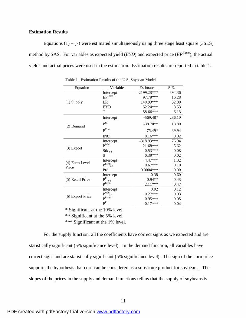
Equations (1) – (7) were estimated simultaneously using three stage least square (3SLS)

method by SAS. For variables as expected yield (EYD) and expected price (EPFarm), the actual

yields and actual prices were used in the estimation. Estimation results are reported in table 1.

Table 1. Estimation Results of the U.S. Soybean Model

Equation Variable Estimate S.E. Intercept -2199.28*** 394.36 EPFarm 97.79*** 16.28 LR 140.93*** 32.80 EYD 52.24*** 8.53

(1) Supply

T 58.66*** 6.13 Intercept -569.48* 286.10 PRtl -38.70** 18.80 PCorn 75.49* 39.94

(2) Demand

INC 0.16*** 0.02 Intercept -318.93*** 76.94 PWld 21.68*** 5.62 Stk t-1 0.53*** 0.08 (3) Export

S 0.39*** 0.02 Intercept 4.47*** 1.32 PFarm

t-1 0.67*** 0.10 (4) Farm Level Price Prd 0.0004*** 0.00

Intercept -0.38 0.60 PRtl

t-1 -0.94** 0.43 (5) Retail Price PFarm 2.11*** 0.47 Intercept 0.02 0.12 PWld

t-1 0.27*** 0.03 PFarm 0.95*** 0.05 (6) Export Price

PRtl -0.17*** 0.04 * Significant at the 10% level. ** Significant at the 5% level. *** Significant at the 1% level.

For the supply function, all the coefficients have correct signs as we expected and are

statistically significant (5% significance level). In the demand function, all variables have

correct signs and are statistically significant (5% significance level). The sign of the corn price

supports the hypothesis that corn can be considered as a substitute product for soybeans. The

slopes of the prices in the supply and demand functions tell us that the supply of soybeans is



12

more elastic than the demand for soybeans with respect to price changes. Equation (4) shows

that the U.S. farm level price is negatively related to soybean output. This means that

overproduction leads to a fall in the farm level price. Equation (6) tells us that the U.S. export

price is positively related to the U.S. farm level price and negatively related to the retail price.

Economic Welfare Analyses for the U.S. Soybean Industry

Given the above estimation results, economic welfare analyses of the U.S. soybean

industry can be conducted.

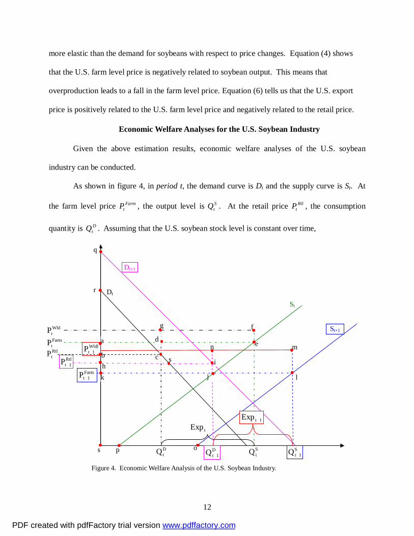
As shown in figure 4, in period t, the demand curve is Dt and the supply curve is St. At

the farm level price FarmtP , the output level is S

tQ . At the retail price RtltP , the consumption

quantity is DtQ . Assuming that the U.S. soybean stock level is constant over time,

n

StQ D

tQ

h

s

s

p o

Farm1tP +

FarmtP RtltP

WldtP

a e

f

b c

d

g

S1tQ +

Rtl1tP +

D1tQ +

Wldl1tP +

i

j k l

m

Dt

Dt+1

St

St+1

tExp 1tExp +

Figure 4. Economic Welfare Analysis of the U.S. Soybean Industry.

q

r



13

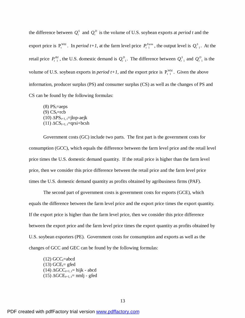
the difference between StQ and D

tQ is the volume of U.S. soybean exports at period t and the

export price is WldtP . In period t+1, at the farm level price Farm

tP 1+ , the output level is StQ 1+ . At the

retail price RtltP 1+ , the U.S. domestic demand is D

tQ 1+ . The difference between StQ 1+ and D

tQ 1+ is the

volume of U.S. soybean exports in period t+1, and the export price is Wld1tP + . Given the above

information, producer surplus (PS) and consumer surplus (CS) as well as the changes of PS and

CS can be found by the following formulas:

(8) PSt=aeps (9) CSt=rcb (10) ∆PSt+1, t=jlop-aejk (11) ∆CSt+1, t=qrsi+bcsh

Government costs (GC) include two parts. The first part is the government costs for

consumption (GCC), which equals the difference between the farm level price and the retail level

price times the U.S. domestic demand quantity. If the retail price is higher than the farm level

price, then we consider this price difference between the retail price and the farm level price

times the U.S. domestic demand quantity as profits obtained by agribusiness firms (PAF).

The second part of government costs is government costs for exports (GCE), which

equals the difference between the farm level price and the export price times the export quantity.

If the export price is higher than the farm level price, then we consider this price difference

between the export price and the farm level price times the export quantity as profits obtained by

U.S. soybean exporters (PE). Government costs for consumption and exports as well as the

changes of GCC and GEC can be found by the following formulas:

(12) GCCt=abcd (13) GCEt= gfed (14) ∆GCCt+1, t= hijk - abcd (15) ∆GCEt+1, t= nmlj - gfed



14

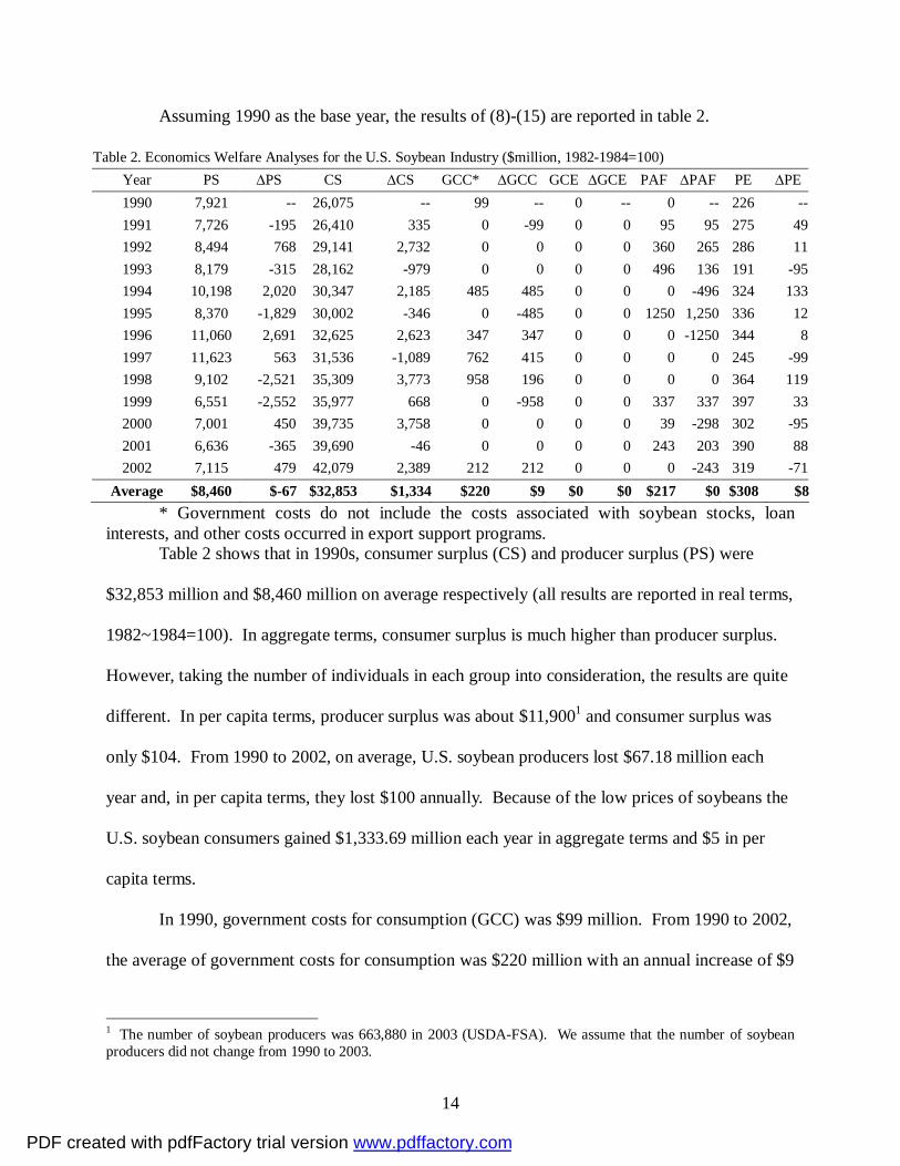
Assuming 1990 as the base year, the results of (8)-(15) are reported in table 2.

Table 2. Economics Welfare Analyses for the U.S. Soybean Industry ($million, 1982-1984=100) Year PS ∆PS CS ∆CS GCC* ∆GCC GCE ∆GCE PAF ∆PAF PE ∆PE 1990 7,921 -- 26,075 -- 99 -- 0 -- 0 -- 226 -- 1991 7,726 -195 26,410 335 0 -99 0 0 95 95 275 49 1992 8,494 768 29,141 2,732 0 0 0 0 360 265 286 11 1993 8,179 -315 28,162 -979 0 0 0 0 496 136 191 -95 1994 10,198 2,020 30,347 2,185 485 485 0 0 0 -496 324 133 1995 8,370 -1,829 30,002 -346 0 -485 0 0 1250 1,250 336 12 1996 11,060 2,691 32,625 2,623 347 347 0 0 0 -1250 344 8 1997 11,623 563 31,536 -1,089 762 415 0 0 0 0 245 -99 1998 9,102 -2,521 35,309 3,773 958 196 0 0 0 0 364 119 1999 6,551 -2,552 35,977 668 0 -958 0 0 337 337 397 33 2000 7,001 450 39,735 3,758 0 0 0 0 39 -298 302 -95 2001 6,636 -365 39,690 -46 0 0 0 0 243 203 390 88 2002 7,115 479 42,079 2,389 212 212 0 0 0 -243 319 -71

Average $8,460 $-67 $32,853 $1,334 $220 $9 $0 $0 $217 $0 $308 $8* Government costs do not include the costs associated with soybean stocks, loan

interests, and other costs occurred in export support programs. Table 2 shows that in 1990s, consumer surplus (CS) and producer surplus (PS) were

$32,853 million and $8,460 million on average respectively (all results are reported in real terms,

1982~1984=100). In aggregate terms, consumer surplus is much higher than producer surplus.

However, taking the number of individuals in each group into consideration, the results are quite

different. In per capita terms, producer surplus was about $11,9001 and consumer surplus was

only $104. From 1990 to 2002, on average, U.S. soybean producers lost $67.18 million each

year and, in per capita terms, they lost $100 annually. Because of the low prices of soybeans the

U.S. soybean consumers gained $1,333.69 million each year in aggregate terms and $5 in per

capita terms.

In 1990, government costs for consumption (GCC) was $99 million. From 1990 to 2002,

the average of government costs for consumption was $220 million with an annual increase of $9

1 The number of soybean producers was 663,880 in 2003 (USDA-FSA). We assume that the number of soybean producers did not change from 1990 to 2003.



15

million in the past twelve years. These government costs were paid by taxpayers. On the other

hand, from 1990 to 2002, on average, U.S. soybean agribusiness firms made a profit (PAF) of

$217 million each year.

Since 1990, U.S. soybean export prices were always higher than U.S. soybean farm level

prices. Therefore government costs were realized. Due to high export prices, in 1990, U.S.

soybean export firms made a profit (PE) of $226 million. From 1990 to 2002, on average, U.S.

soybean export firms made a profit of $308 million each year with an annual increase of $8

million.

Due to the unavailability of the number of U.S. soybean business firms and U.S. soybean

exporters, the per capita gain can not be calculated directly. Assuming the number of

agribusiness firms and exporters is 10% of U.S. producers, in per capita terms, on average

agribusiness firms made a profit of $3,268 each year and exporters made a profit of $4,635.

In summary, in aggregate terms the descending order of the benefits obtained by different

interest groups in the U.S. soybean industry is: consumers, producers, exporters, agribusinesses,

and taxpayers. In per capita terms, the descending order of the benefits obtained by different

interest groups is: producers, exporters, agribusinesses, consumers, and taxpayers. These

differences stem from the number of individuals in each group, i.e., there are a large number of

taxpayers and consumers, and relatively small number of producers, agribusiness firms, and

export firms. Comparing the changes of the benefits obtained by different interest groups over

the past 12 years, producers and taxpayers were losing money, exporters were gaining more and

more profits, the profits of agribusinesses were stable, and consumers were benefited because of

the low price of soybeans.



16

Conclusions

The soybean industry is a crucial sector for U.S. agriculture. U.S. soybeans have been a

subsidized commodity since 1941 and the 2002 Farm Bill provides direct government and

counter-cyclical payments for the first time. The 2002 target price for soybeans was set at

$5.80/bushel, which was expected to be effective through 2007. This research developed a

soybean industry level model and conducted welfare economic analyses on the U.S. soybean

industry. Results indicate that in the last 12 years, in aggregate terms U.S. consumers dominated

other interest groups in the U.S. soybean industry. However, in per capita terms, U.S. soybean

producers were the dominant interest group, although their benefits declined gradually. U.S.

exporters and agribusiness firms also took profitable positions in the U.S. soybean industry while

taxpayers paid for the government costs associated with U.S. soybean subsidy policies.

References

American Soybean Association. Farm Bill Summary (Key Soybean in the 2002 Farm Bill), Website: http://www.soystats.com/2002/page_37.htm.

Executive Office of the President. "Economic Report of the President (2003)." Website: http://w3.access.gpo.gov/usbudget/fy2004/erp.html

Food and Agriculture Organization of the United Nations (FAO). Online statistics databases, 2003. Website: http://apps.fao.org/page/collections?subset=agriculture.

Gardner, Bruce L. "The Why, How, and Consequences of Agricultural Polices." Agricultural Protectionism in the industrialized world, the National Center for Food and Agricultural Policy at Resources for the Future, 1990.

Piggott, Nick, Michael Wohlgenant, Kelly Zering, and Steve Sonka. "Analysis of the Economic Importance of Changes in Soybean Use." The National Soybean Research Laboratory, 2000. Website: http://www.nsrl.uiuc.edu/Econom.pdf.

Reed, Albert J., Howard Elitzak, and Michael K. Wohlgenant. "Retail-Farm Price Margins and Consumer Product Diversity." Washington, D.C. USDA-ERS Technical Bulletin No. TB1899. pp 29, April 2002.


http://www.soystats.com/2002/page_37.htm

http://w3.access.gpo.gov/usbudget/fy2004/erp.html

http://apps.fao.org/page/collections?subset=agriculture

http://www.nsrl.uiuc.edu/Econom.pdf


17

Schnepf, Randall D., Erik Dohlman, and Christine Bolling. "Agriculture in Brazil and Argentina: Developments and Prospects for Major Fild Crops." Washington, D.C. USDA-ERS, WRS-01-3, Nov. 2001.

U.S. Department of Agriculture, Economic Research Service (USDA-ERS). Data (Online), 2004. Website: http://www.ers.usda.gov/Data/

U.S. Department of Agriculture, Farm Service Agency (USDA-FSA), 2004. Website: http://www.fsa.usda.gov/pas/

U.S. Department of Agriculture, Foreign Agriculture Service (USDA-FAS). Production, Supply and Demand online databases, 2004. Website: http://www.fas.usda.gov/psd/complete_files/default.asp.

Westcott, Paul C., and J. Michael Price. "Impacts of the U.S. Marketing Loan Program for Soybeans." Washington, D.C. USDA-ERS, Oil Crops Situation and Outlook, OCS-1999, Oct. 1999.

Westcott, Paul C., and J. Michael Price. "Analysis of the U.S. Commodity Loan Program with Marketing Loan." Washington, D.C. USDA-ERS Report No. 801, Apr. 2001.


http://www.ers.usda.gov/Data/

http://www.fsa.usda.gov/pas/

http://www.fas.usda.gov/psd/complete_files/default.asp



Baohui Song Research Assistant University of Kentucky Department of Agricultural Economics 417 C. E. Barnhart Bldg. Lexington, KY 40546-0276 Phone: (859) 257-7283 Fax: (859) 257-7290 E-mail: [email protected] Shuang Xu Research Assistant University of Kentucky Department of Agricultural Economics 417 C. E. Barnhart Bldg. Lexington, KY 40546-0276 Phone: (859) 257-7283 Fax: (859) 257-7290 E-mail: [email protected]

Mary A. Marchant Professor University of Kentucky Department of Agricultural Economics 314 C. E. Barnhart Bldg. Lexington, KY 40546-0276 Phone: (859) 257-7260 Fax: (859) 257-7290 E-mail: [email protected]

Selected Paper prepared for presentation at the American Agricultural Economics Association

Annual Meeting, Denver, Colorado, August 1-4, 2004

Copyright 2004 by Baohui Song, Mary A. Marchant, and Shuang Xu. All rights reserved. Readers may make verbatim copies of this document for non-commercial purposes by any means, provided that this copyright notice appears on all such copies.






1


Abstract

Globally the U.S. is the number one producer, consumer and exporter of soybeans.

Nationally, U.S. soybean production value ranks second among all agricultural bulk

commodities, having a significant impact on U.S. farm incomes. U.S. soybean has been a

subsidized commodity since 1941 and the 2002 Farm Bill provides soybeans for the first time

direct government payment and counter-cyclical payments. Using welfare economics, this

research explores the political economy of U.S. soybean subsidy policies. Results for the U.S.

soybean industry indicate that in aggregate terms, consumer interests dominate and in per capita

terms, producer interests dominate.

Introduction

An Overview of U.S. Soybeans

The soybean industry in the U.S. plays an important role in the world. Globally, the U.S.

is the leading country in soybean production, consumption and exports as shown in figure 1-a,

figure 1-b, and figure 1-c. These three figures also show that in the last decade, Brazil and

Argentina have become major competitors for the U.S. in the world soybean market (Schnefp,

Dohlman, and Bolling, 2001). In 2003, U.S. soybean production was 65.80 million metric tons,

accounting for 35% of world production; U.S. soybean consumption was 43.25 million metric

tons, 21.68% of world consumption; and U.S. soybean exports were 24.49 million metric tons,

39.07% of world exports (FAO, 2004). However, U.S. soybean imports were very low, only 0.22

million metric tons in 2003 (USDA-FAS, 2004).



2

Figure 1-a. Soybean Production Comparison between the U.S. and other Countries. Source: FAO, online statistical databases, 2004.

Figure 1-b. Soybean Consumption Comparison between the U.S. and Other Countries. Source: USDA-FAS, PS&D online dataset, 2004.

65.80

51.55

34.80

16.50

20.88

0

50

100

150

200

1964 1967 1970 1973 1976 1979 1982 1985 1988 1991 1994 1997 2000 2003

(Mill

ion

Met

ric T

ons)

s


57.62

43.25

37.89

34.95

25.80

0

50

100

150

200

1964 1967 1970 1973 1976 1979 1982 1985 1988 1991 1994 1997 2000 2003

(Mill

ion

Met

ric T

ons)

.

Others the U.S. China Brazil Argentina



3

Figure 1-c. Soybean Export Comparison between U.S. and Other Countries. Source: USDA-FAS, PS&D online dataset, 2004.

Nationally, the soybean industry is a crucial sector in U.S. agriculture. U.S. soybean

production value was $16.18 billion in 2002/2003, ranking second among all agricultural bulk

commodities. Since 2000, soybeans have been U.S.’s leading agricultural export for agricultural

bulk commodities, exceeding corn and wheat. Soybeans have been one of the U.S. government-

supported commodities since 1941. Before the 2002 Farm Bill, the primary government support

programs for soybeans included commodity loan and marketing loan programs. Under these

programs, government payments for the soybean industry increased quickly, especially in the last

decade. The net government expenditures on the soybean subsidy program were - $86 million in

1990 and increased to $3,281 million in 2001 (USDA-FSA, 2004). Even with the increasing

subsidy burden, the 2002 Farm Bill further placed soybeans under the direct payment and the

counter-cyclical payment programs, and set $5.80/bushel as the target price through 2007

(American Soybean Association, 2002).

24.49

23.50

10.25

0.28

4.17

0

25

50

75

1965 1967 1969 1971 1973 1975 1977 1979 1981 1983 1985 1987 1989 1991 1993 1995 1997 1999 2001 2003

(Mill

ion

Met

ric T

ons)

s




4

Objectives

In this research, our objectives include 1) developing a soybean model at the industry

level, which incorporates endogenous supply, demand and prices and other related exogenous

variables; 2) estimating the model as a simultaneous equation system; 3) conducting economics

welfare analyses for the U.S. soybean industry; 4) identifying which interest group dominates the

U.S. soybean industry.

U.S. Government Soybean Subsidy Programs

The main U.S. soybean subsidy programs include soybean loan program and government

payments. The soybean loan program was first introduced in 1941 and has been in place since

then, except in 1975 (Westcott and Price, 2001). The original form of the soybean loan program

was the commodity loan program, which supported the market price. The marketing loan

program started in the mid-1980s, which mainly supported producers’ income instead of the

market prices.

Under the commodity loan program, producers must keep the crop designated as loan

collateral in approved storage to preserve the crop’s quality. Producers may choose to either

default on the loan at the end of the loan period, keeping the loan money and forfeiting

ownership of collateral to the government or sell the commodity and repay the loan plus interest,

depending on the market price level (Westcott and Price, 1999). While under the marketing loan

program producers may operate as described above. Alternatively, the marketing loan provisions

also allow repayment of commodity loans at less than the original loan rate when market prices

are lower (USDA-ERS, 2004). This feature decreases the loan program’s potential effect on

supporting prices because stock accumulation by the government, through loan defaults, is

reduced. Instead, farmers are provided economic incentives to retain ownership of the crops and



5

sell them rather than default on loans and forfeit ownership of the crops to the government

(Westcott and Price, 1999).

Another subsidy form for soybeans is government payments, including direct payments

and counter-cyclical payments within the 2002 Farm Bill. The formula for direct payments is:

Direct Payment = Base Acres x Program Yield x 85% x Direct Payment Rate

Base acres and program yields are calculated on the average level of the recent history of

planted acres and yields, while the direct payment rate (DPR) is decided by the USDA. The

2002 Farm Bill set the DPR for soybeans at $0.44/bushel. Direct payments only relate to the

planted area, so farmers and eligible landowners will receive annual direct payments.

The Counter-Cyclical Payments formula is:

Counter-Cyclical Payment=Base Acres × Program Yield × 85% × CCP Rate CCP Rate = Max (0, Target Price – Effective Price) Effective Price = Max (MYA Price, Loan Rate) + Direct Payment Rate

The MYA price is the marketing year average price, and the 2002 Farm Bill set the target

price for soybeans at $5.80/bushel. The counter-cyclical payment is closely related to the market

price. If the market price is high enough, the counter-cyclical payment will not occur.

Literature Review

In modeling the soybean industry, different methods have been employed. Piggott et al.

(2000), estimated soybeans, soybean meal and soybean oil demand and supply elasticities using

1974 to 1998 annual data. The cross effect between supply and demand could not be examined

because they estimated the demand and supply independently. Since they used the domestic

disappearance as the total demand, the effects of some exogenous factors on soybean supply and

demand cannot be examined. The USDA also has its own estimation model to predict the supply

and demand (Reed, et al., 2002). Given the estimated elasticities and baseline demand and prices,



6

they estimate the demand using a system of equations, including export demand, feed demand,

crushing demand, industrial demand, domestic demand, food demand, etc. Similar methods

were used for the supply side. Gardner (1990) used cross elasticities (among wheat, corn and

soybeans), estimated by Tyers and Anderson and Johnson et al., to determine producers’ gains

and losses. However, many previous works did not incorporate exports as an endogenous

variable in the model. The U.S. is the biggest soybean exporter in the world, and in 2003 U.S.

soybean exports comprised 37% of U.S. soybean output (USDA-FAS, 2004). The empirical

estimation results might not be reliable when the export effect on the U.S. soybean industry was

ignored. Modeling the Soybeans Industry

The Structure of the U.S. Soybean Industry

To accurately describe the U.S. soybean industry, the structure of the demand and supply

system and the factors that will affect the system were introduced first. As shown in Figure 3,

the entire soybean industry can be viewed as interaction of four components: supply, demand,

prices and exogenous factors.

Supply comes from three sources: production, beginning stocks and imports. Demand

includes four parts: crush demand, export demand, stocks, and others, among them the crushed

soybeans can be further divided into the sub-categories of soybean oil and soybean meal.

Soybean oil and soybean meal can be allocated based on usage into domestic consumption,

exports, and stocks. Three levels of soybean price---farm-level prices, retail-level prices and

world prices are taken into consideration as price variables. Seven defined exogenous variables

are included in this system. Technology, production cost, government subsidy and yield affect

the producer’s decision on outputs. Corn price (hypothesizing that corn is a substitute product

for soybeans), disposable personal income and population affect the total demand.



7

Production

Stocks

Imports

Farmer Price

Market Price

Figure 2. Structural Diagram of the U.S. Soybean Industry.

World Price

Consumption

Exports Crush

Exports

Other

Oil

Meal

Other Stocks

Stocks

Exogenous

Population

Income Subsidies

Others

Cost

Yield

Supplies Demands Price

Exogenous

Corn Price

Others Tech

Endogenous



8

Theoretical Model

From the above structure, the model of U.S. soybean industry can be expressed as below:

(1) S=f(EPFarm, Stk, LR, EYD, Tech, Cost, Others) (2) D=g(PRtl, PCorn, INC, POP, Others) (3) E=h(STK, S, D, Others) (4) PFarm=φ( Farm

tP 1− , GS, S, Others) (5) PRtl=ψ(PFarm, Others) (6) PWld=π( Wld

tP 1− ,E, Others) (7) Stk =( 1tStk − , M*, E, D)

* Since U.S. soybean imports were quite small, we do not include import equation in the model.

Where S: Supply of soybeans; EPFarm: Expected farm-level prices; LR: Loan rates of soybeans; EYD: Expected yields; Stk: Domestic stocks of soybeans; Tech: Technology; Cost: Production costs for soybeans; M: Import;

PRtl: Retail prices for soybeans; PCorn: Retail prices for corn; E: Exports of soybeans; M: U.S. soybean Imports; PWld: World prices for soybeans; INC: Personal disposable income; POP: Population; GS: Government subsidy.

Based on the above analysis, empirical equations are expressed as follows. The expected

signs for the coefficients are shown below the coefficients.

(1) S = 0α + 1α FarmEP + 2α LR + 3α EYD + 4α T (+) (+) (+) (+)

(2) D = 0β + 1β RtlP + 2β cornP + 3β PINC (-) (+) (+)

(3) E = 0γ + 1γ PWld + 2γ 1−tSTK + 3γ S (+) (+) (+)

(4 FarmtP = 0θ + 1θ Farm

tP 1− + 2θ S (+) (-)

(5) RtltP = 0λ + Rtl

tP 11 −λ + 2λ FarmP (+) (+)

(6) WldtP = 0ω + 1ω Wld

tP 1− + 2ω FarmP + 3ω RtlP (+) (+) (-)

(7) tSTK =STKt-1 + S + M – D – E



9

where S: Supply of soybeans, equaling the domestic production (million bushels); EPFarm: Expected prices received by farmers (dollars/bushel); LR: Loan rates of soybeans (dollars/bushel); EYD: Expected soybean yields (bushels/acre); STK: Domestic stocks of soybeans (million bushels); D: Domestic crush demand (million bushels); PFarm: The prices received by farmers (dollars/bushel); PRtl: Retail prices for soybeans (dollars/bushel); PCorn: Retail prices for corn (dollars/bushel); PINC: Per capita personal disposable income (dollars); E: Exports of soybeans (million bushels); M: U.S. soybean imports (million bushels); PWld: World prices for soybeans (dollars/bushel). T: Time trend variable. Equation (1) assumes that the soybean supply (S) is influenced by the following factors:

a) the expected farm level price (EPFarm), based on the assumption that the farmers can easily get

the forecast price information; b) the loan rate (LR), which is normally announced before the

farmers make their decisions; c) expected yield (EYD); and d) a time trend variable (T), which

captures the technology progress. In this equation, costs are not included because correlation

between cost and the time trend variable (0.98) causes a severe multicollinearity problem.

Equation (2) shows that the domestic consumption (D) of soybeans (including waste and

seed) is influenced by: a) the retail price for soybeans (PRtl); b) the price of corn (PCorn), based

on the assumption that corn can be a substitute for soybeans, either in terms of feed usage, oil

usage or in terms of the planting area; and c) U.S. per capita personal disposable income (PINC).

Equation (3) says that exports (E) of soybeans is a function of a) world price (PWld); b)

previous stocks of soybeans (STKt-1); and c) production (S).

Equation (4) expresses that the farm level price (PFarm) is affected by the lagged price

level ( Farm1tP − ), based on the assumption that the lagged price contains information that determines



10

current prices; and b) the domestic supply level (S), based on the assumption that, once the

farmers decide their production level, price will clear the markets. Equation (5) tries to capture

the relationship between the two prices --- retail price (PRtl) and farm level price (PFarm), and we

also assume that the lagged retail price ( RtltP 1− ) has some impact on the current retail price.

Equation (6) tries to show how the world price (PWld) relates to the U.S. soybean retail price and

the U.S. soybean farm level price. We also assume the lagged world price ( WldtP 1− ) will affect the

current world price.

Equation (7) is an identity. It shows that the ending stock level (STKt) equals the

beginning stock level (STKt-1) plus domestic production (S) and import (M) minus domestic

crushing demand (D) and export (E).

Empirical Estimation

Data Description

All data used in this research are annual data from 1965 to 2002. The data of demand,

supply, stock, export and import comes from the USDA-FAS PS&D online databases. The data

of soybean prices is from the USDA-ERS Oil Crops Yearbook. We used the wholesale price of

No. 1 yellow soybean prices in the Chicago Market for the retail price, assuming a constant

margin between wholesale prices and retail prices. The world prices for soybeans are derived

prices---the export value divided by export quantity---from the FAO statistical databases. Corn

prices are the Chicago Market prices for No. 2 yellow corn from the USDA-ERS Feed Yearbook.

The income, population and price indexes data is from the Economic Report of the President

(2003). In addition, all data related to price and incomes are transformed into real terms.

Income has been deflated by the GDP deflator (1982=100). Prices are deflated by the consumer

price index (1982~1984=100).



11

Estimation Results

Equations (1) – (7) were estimated simultaneously using three stage least square (3SLS)

method by SAS. For variables as expected yield (EYD) and expected price (EPFarm), the actual

yields and actual prices were used in the estimation. Estimation results are reported in table 1.

Table 1. Estimation Results of the U.S. Soybean Model

Equation Variable Estimate S.E. Intercept -2199.28*** 394.36 EPFarm 97.79*** 16.28 LR 140.93*** 32.80 EYD 52.24*** 8.53

(1) Supply

T 58.66*** 6.13 Intercept -569.48* 286.10 PRtl -38.70** 18.80 PCorn 75.49* 39.94

(2) Demand

INC 0.16*** 0.02 Intercept -318.93*** 76.94 PWld 21.68*** 5.62 Stk t-1 0.53*** 0.08 (3) Export

S 0.39*** 0.02 Intercept 4.47*** 1.32 PFarm

t-1 0.67*** 0.10 (4) Farm Level Price Prd 0.0004*** 0.00

Intercept -0.38 0.60 PRtl

t-1 -0.94** 0.43 (5) Retail Price PFarm 2.11*** 0.47 Intercept 0.02 0.12 PWld

t-1 0.27*** 0.03 PFarm 0.95*** 0.05 (6) Export Price

PRtl -0.17*** 0.04 * Significant at the 10% level. ** Significant at the 5% level. *** Significant at the 1% level.

For the supply function, all the coefficients have correct signs as we expected and are

statistically significant (5% significance level). In the demand function, all variables have

correct signs and are statistically significant (5% significance level). The sign of the corn price

supports the hypothesis that corn can be considered as a substitute product for soybeans. The

slopes of the prices in the supply and demand functions tell us that the supply of soybeans is



12

more elastic than the demand for soybeans with respect to price changes. Equation (4) shows

that the U.S. farm level price is negatively related to soybean output. This means that

overproduction leads to a fall in the farm level price. Equation (6) tells us that the U.S. export

price is positively related to the U.S. farm level price and negatively related to the retail price.

Economic Welfare Analyses for the U.S. Soybean Industry

Given the above estimation results, economic welfare analyses of the U.S. soybean

industry can be conducted.

As shown in figure 4, in period t, the demand curve is Dt and the supply curve is St. At

the farm level price FarmtP , the output level is S

tQ . At the retail price RtltP , the consumption

quantity is DtQ . Assuming that the U.S. soybean stock level is constant over time,

n

StQ D

tQ

h

s

s

p o

Farm1tP +

FarmtP RtltP

WldtP

a e

f

b c

d

g

S1tQ +

Rtl1tP +

D1tQ +

Wldl1tP +

i

j k l

m

Dt

Dt+1

St

St+1

tExp 1tExp +

Figure 4. Economic Welfare Analysis of the U.S. Soybean Industry.

q

r



13

the difference between StQ and D

tQ is the volume of U.S. soybean exports at period t and the

export price is WldtP . In period t+1, at the farm level price Farm

tP 1+ , the output level is StQ 1+ . At the

retail price RtltP 1+ , the U.S. domestic demand is D

tQ 1+ . The difference between StQ 1+ and D

tQ 1+ is the

volume of U.S. soybean exports in period t+1, and the export price is Wld1tP + . Given the above

information, producer surplus (PS) and consumer surplus (CS) as well as the changes of PS and

CS can be found by the following formulas:

(8) PSt=aeps (9) CSt=rcb (10) ∆PSt+1, t=jlop-aejk (11) ∆CSt+1, t=qrsi+bcsh

Government costs (GC) include two parts. The first part is the government costs for

consumption (GCC), which equals the difference between the farm level price and the retail level

price times the U.S. domestic demand quantity. If the retail price is higher than the farm level

price, then we consider this price difference between the retail price and the farm level price

times the U.S. domestic demand quantity as profits obtained by agribusiness firms (PAF).

The second part of government costs is government costs for exports (GCE), which

equals the difference between the farm level price and the export price times the export quantity.

If the export price is higher than the farm level price, then we consider this price difference

between the export price and the farm level price times the export quantity as profits obtained by

U.S. soybean exporters (PE). Government costs for consumption and exports as well as the

changes of GCC and GEC can be found by the following formulas:

(12) GCCt=abcd (13) GCEt= gfed (14) ∆GCCt+1, t= hijk - abcd (15) ∆GCEt+1, t= nmlj - gfed



14

Assuming 1990 as the base year, the results of (8)-(15) are reported in table 2.

Table 2. Economics Welfare Analyses for the U.S. Soybean Industry ($million, 1982-1984=100) Year PS ∆PS CS ∆CS GCC* ∆GCC GCE ∆GCE PAF ∆PAF PE ∆PE 1990 7,921 -- 26,075 -- 99 -- 0 -- 0 -- 226 -- 1991 7,726 -195 26,410 335 0 -99 0 0 95 95 275 49 1992 8,494 768 29,141 2,732 0 0 0 0 360 265 286 11 1993 8,179 -315 28,162 -979 0 0 0 0 496 136 191 -95 1994 10,198 2,020 30,347 2,185 485 485 0 0 0 -496 324 133 1995 8,370 -1,829 30,002 -346 0 -485 0 0 1250 1,250 336 12 1996 11,060 2,691 32,625 2,623 347 347 0 0 0 -1250 344 8 1997 11,623 563 31,536 -1,089 762 415 0 0 0 0 245 -99 1998 9,102 -2,521 35,309 3,773 958 196 0 0 0 0 364 119 1999 6,551 -2,552 35,977 668 0 -958 0 0 337 337 397 33 2000 7,001 450 39,735 3,758 0 0 0 0 39 -298 302 -95 2001 6,636 -365 39,690 -46 0 0 0 0 243 203 390 88 2002 7,115 479 42,079 2,389 212 212 0 0 0 -243 319 -71

Average $8,460 $-67 $32,853 $1,334 $220 $9 $0 $0 $217 $0 $308 $8* Government costs do not include the costs associated with soybean stocks, loan

interests, and other costs occurred in export support programs. Table 2 shows that in 1990s, consumer surplus (CS) and producer surplus (PS) were

$32,853 million and $8,460 million on average respectively (all results are reported in real terms,

1982~1984=100). In aggregate terms, consumer surplus is much higher than producer surplus.

However, taking the number of individuals in each group into consideration, the results are quite

different. In per capita terms, producer surplus was about $11,9001 and consumer surplus was

only $104. From 1990 to 2002, on average, U.S. soybean producers lost $67.18 million each

year and, in per capita terms, they lost $100 annually. Because of the low prices of soybeans the

U.S. soybean consumers gained $1,333.69 million each year in aggregate terms and $5 in per

capita terms.

In 1990, government costs for consumption (GCC) was $99 million. From 1990 to 2002,

the average of government costs for consumption was $220 million with an annual increase of $9

1 The number of soybean producers was 663,880 in 2003 (USDA-FSA). We assume that the number of soybean producers did not change from 1990 to 2003.



15

million in the past twelve years. These government costs were paid by taxpayers. On the other

hand, from 1990 to 2002, on average, U.S. soybean agribusiness firms made a profit (PAF) of

$217 million each year.

Since 1990, U.S. soybean export prices were always higher than U.S. soybean farm level

prices. Therefore government costs were realized. Due to high export prices, in 1990, U.S.

soybean export firms made a profit (PE) of $226 million. From 1990 to 2002, on average, U.S.

soybean export firms made a profit of $308 million each year with an annual increase of $8

million.

Due to the unavailability of the number of U.S. soybean business firms and U.S. soybean

exporters, the per capita gain can not be calculated directly. Assuming the number of

agribusiness firms and exporters is 10% of U.S. producers, in per capita terms, on average

agribusiness firms made a profit of $3,268 each year and exporters made a profit of $4,635.

In summary, in aggregate terms the descending order of the benefits obtained by different

interest groups in the U.S. soybean industry is: consumers, producers, exporters, agribusinesses,

and taxpayers. In per capita terms, the descending order of the benefits obtained by different

interest groups is: producers, exporters, agribusinesses, consumers, and taxpayers. These

differences stem from the number of individuals in each group, i.e., there are a large number of

taxpayers and consumers, and relatively small number of producers, agribusiness firms, and

export firms. Comparing the changes of the benefits obtained by different interest groups over

the past 12 years, producers and taxpayers were losing money, exporters were gaining more and

more profits, the profits of agribusinesses were stable, and consumers were benefited because of

the low price of soybeans.



16

Conclusions

The soybean industry is a crucial sector for U.S. agriculture. U.S. soybeans have been a

subsidized commodity since 1941 and the 2002 Farm Bill provides direct government and

counter-cyclical payments for the first time. The 2002 target price for soybeans was set at

$5.80/bushel, which was expected to be effective through 2007. This research developed a

soybean industry level model and conducted welfare economic analyses on the U.S. soybean

industry. Results indicate that in the last 12 years, in aggregate terms U.S. consumers dominated

other interest groups in the U.S. soybean industry. However, in per capita terms, U.S. soybean

producers were the dominant interest group, although their benefits declined gradually. U.S.

exporters and agribusiness firms also took profitable positions in the U.S. soybean industry while

taxpayers paid for the government costs associated with U.S. soybean subsidy policies.

References

American Soybean Association. Farm Bill Summary (Key Soybean in the 2002 Farm Bill), Website: http://www.soystats.com/2002/page_37.htm.

Executive Office of the President. "Economic Report of the President (2003)." Website: http://w3.access.gpo.gov/usbudget/fy2004/erp.html

Food and Agriculture Organization of the United Nations (FAO). Online statistics databases, 2003. Website: http://apps.fao.org/page/collections?subset=agriculture.

Gardner, Bruce L. "The Why, How, and Consequences of Agricultural Polices." Agricultural Protectionism in the industrialized world, the National Center for Food and Agricultural Policy at Resources for the Future, 1990.

Piggott, Nick, Michael Wohlgenant, Kelly Zering, and Steve Sonka. "Analysis of the Economic Importance of Changes in Soybean Use." The National Soybean Research Laboratory, 2000. Website: http://www.nsrl.uiuc.edu/Econom.pdf.

Reed, Albert J., Howard Elitzak, and Michael K. Wohlgenant. "Retail-Farm Price Margins and Consumer Product Diversity." Washington, D.C. USDA-ERS Technical Bulletin No. TB1899. pp 29, April 2002.


http://www.soystats.com/2002/page_37.htm

http://w3.access.gpo.gov/usbudget/fy2004/erp.html

http://apps.fao.org/page/collections?subset=agriculture

http://www.nsrl.uiuc.edu/Econom.pdf


17

Schnepf, Randall D., Erik Dohlman, and Christine Bolling. "Agriculture in Brazil and Argentina: Developments and Prospects for Major Fild Crops." Washington, D.C. USDA-ERS, WRS-01-3, Nov. 2001.

U.S. Department of Agriculture, Economic Research Service (USDA-ERS). Data (Online), 2004. Website: http://www.ers.usda.gov/Data/

U.S. Department of Agriculture, Farm Service Agency (USDA-FSA), 2004. Website: http://www.fsa.usda.gov/pas/

U.S. Department of Agriculture, Foreign Agriculture Service (USDA-FAS). Production, Supply and Demand online databases, 2004. Website: http://www.fas.usda.gov/psd/complete_files/default.asp.

Westcott, Paul C., and J. Michael Price. "Impacts of the U.S. Marketing Loan Program for Soybeans." Washington, D.C. USDA-ERS, Oil Crops Situation and Outlook, OCS-1999, Oct. 1999.

Westcott, Paul C., and J. Michael Price. "Analysis of the U.S. Commodity Loan Program with Marketing Loan." Washington, D.C. USDA-ERS Report No. 801, Apr. 2001.


http://www.ers.usda.gov/Data/

http://www.fsa.usda.gov/pas/

http://www.fas.usda.gov/psd/complete_files/default.asp


Documents

Who Dominates the U.S. Soybean Industry: Producers ...ageconsearch.umn.edu/bitstream/20117/1/sp04so02.pdf · Who Dominates the U.S. Soybean Industry: Producers, Consumers, or Agribusinesses?