Who Lives on the Wrong Side of the Environmental … · 2016-11-12 · highlight the importance of controlling for interregional variation in pollution levels ... regional variations

Who Lives on the Wrong Side of theEnvironmental Tracks? Evidence fromthe EPA’s Risk-Screening EnvironmentalIndicators Modeln

Michael Ash, University of Massachusetts, Amherst

T. Robert Fetter, Science Applications International Corporation (SAIC)

Objective. We analyze the social and economic correlates of air pollution exposurein U.S. cities. Methods. We combine 1990 Census block group data for urbanizedareas with 1998 data on toxicity-adjusted exposure to air pollution. Using a uniquedata set created as a byproduct of the EPA’s Risk-Screening EnvironmentalIndicators Model, we improve on previous studies of environmental inequality inthree ways. First, where previous studies focus on the proximity to point sourcesand the total mass of pollutants released, our measure of toxic exposure reflectsatmospheric dispersion and chemical toxicity. Second, we analyze the data at a finelevel of geographic resolution. Third, we control for substantial regional variationsin pollution, allowing us to identify exposure differences both within cities andbetween cities. Results. We find that African Americans tend to live both in morepolluted cities in the United States and in more polluted neighborhoods withincities. Hispanics live in less polluted cities on average, but they live in more pollutedareas within cities. We find an extremely consistent income-pollution gradient, withlower-income people significantly more exposed to pollution. Conclusions. Com-munities with higher concentrations of lower-income people and people of colorexperience disproportionate exposure to environmental hazards. Our findingshighlight the importance of controlling for interregional variation in pollution levelsin studies of the demographic correlates of pollution.

The study of environmental justice examines differential availability ofenvironmental amenities or exposure to environmental disamenities on thebasis of socioeconomic, ethnic, or racial difference. Under alternative defini-tions of environmental justice, inequality may itself constitute injustice, orthe cause of the inequality may matter as well. Even on the straightforward

nDirect correspondence to Michael Ash, Department of Economics, University ofMassachusetts, Amherst, MA 01003 [email protected]. Ash will provide all data andcoding information to those wishing to replicate the study. Ash and Fetter are equal co-authors. We thank James Boyce and John Stranlund for their invaluable guidance, and we aredeeply grateful to Nicolaas W. Bouwes and Steven M. Hassur of the EnvironmentalProtection Agency who painstakingly developed and graciously provided us with access to theRisk-Screening Environmental Indicators data.

SOCIAL SCIENCE QUARTERLY, Volume 85, Number 2, June 2004r2004 by the Southwestern Social Science Association

question of what social attributes correlate with environmental quality,researchers disagree about methodology and findings. Using different indi-cators of environmental disamenities, units of spatial analysis, explanatoryvariables, and theoretical frameworks, researchers have found evidence forwidely different conclusions.

With respect to recurrent themes in recent analyses, we contribute threemethodological improvements. First, we use a realistic indicator of pollutionexposure that is based on the U.S. Environmental Protection Agency’sToxics Release Inventory (TRI) but takes into account relative toxicity andchemical fate and transport. Second, we examine correlations at geogra-phically small units, Census block groups, to avoid the ecological fallacy,that is, reaching conclusions from a large unit of analysis that do not hold atsmaller resolution due to spatial heterogeneity. Third, we incorporateregional variations into a national analysis in a novel way.

Across all cities in the contiguous United States, we find that neigh-borhoods with higher proportions of African Americans tend to experiencehigher levels of toxicity-adjusted exposure to air pollution from TRI-reporting facilities than do predominantly white neighborhoods, whereasneighborhoods with higher proportions of Hispanics tend to experiencelower levels of pollution. However, a model that compares neighborhoods inthe same city shows that neighborhoods with more Hispanics and those withmore African Americans have more pollution on average. Taken together,these results imply that African Americans tend to live in more pollutedcities than do whites, and also tend to live in more polluted neighborhoodswithin cities. Although Hispanics tend to live in less polluted cities than dowhites, they too live in more polluted neighborhoods within cities.

Literature Review

In this section, we survey recent practice in the environmental justiceliterature, with particular focus on the areas in which we offer metho-dological improvements. We then briefly address the conventional practicesthat we follow.

Choice of Pollution Indicator

Many studies of the demographic correlates of pollution use as thedependent variable the presence or absence of a polluting facility, suchas a toxic storage and disposal facility (TSDF) (e.g., United Church ofChrist, 1987; Mohai and Bryant, 1992; Anderton et al., 1994; Oakes, 1997;Been and Gupta, 1997; Boer et al., 1997; Pastor, 2001). The presenceof a polluting facility in a neighborhood has validity as an indicator ofenvironmental quality, especially as perceived by residents, but imprecisely

442 Social Science Quarterly

measures exposure to hazard. The mass of pollutants released withincommunity borders better proxies environmental quality, and most studiesthat use TRI data focus on the mass of toxic releases, for example, Bowenet al. (1995), Kriesel, Centner, and Keeler (1996), and Arora and Cason(1999).

Recognizing that mass of pollutants released within neighborhoodsremains a blunt measure of environmental quality, some researchers haveadjusted TRI data for toxicity and dispersion. Glickman and Hersh (1995)estimate risks from chronic exposure to industrial facilities in AlleghanyCounty, Pennsylvania. Using TRI and other data, adjusted for toxicity andwind patterns, they find that Census block groups with more AfricanAmericans, poor people, and people over age 65 face higher risks comparedto the rest of the population. In a high-resolution study of TRI releases inDes Moines, Iowa, Chakraborty and Armstrong (1997) show that plume-based models of dispersion reveal higher exposure of African Americans andpoor people. McMaster, Leitner, and Sheppard (1997) demonstrate thatfiner geographic resolution and toxicity adjusting predict higher exposure ofpoor people to TRI releases in Minneapolis. Using TRI releases adjusted forchronic health effects and distance from pollution source, Brooks and Sethi(1997) find that zip codes with more African Americans experience greaterpollution. The relationship holds even when income, education, urbaniza-tion, housing value, manufacturing employment, and population density areheld constant. Using an index based on TRI releases, adjusted for toxicityand accounting for chemical fate and transport using EPA-reviewed modelsand databases, Bouwes, Hassur, and Shapiro (2001) find that denselypopulated square-kilometer neighborhoods with more African Americans,Hispanics, Asians, and unemployed residents tend to be more polluted thanother densely populated neighborhoods.

Unit of Spatial Analysis

The unit of spatial analysis may significantly affect findings. One of thefirst studies to receive national attention (United Church of Christ, 1987)compares the demographics of zip codes containing commercial TSDFs tothose of zip codes without TSDFs. Hird and Reese (1998) exploredemographic correlations with 29 indicators of environmental quality at thecounty level. Brooks and Sethi (1997) use a sophisticated indicator ofpollution, but define neighborhoods as zip codes. Such studies may sufferfrom ecological fallacy: correlations identified at large units of analysis maynot hold at finer resolution. Most researchers would probably agree in theabstract that ‘‘the area chosen for analysis should correspond to the likelyareal distribution of possible harm’’ (Anderton et al., 1994:128).Uncertainty about the range of possible harm from point sources makesdifficult the precise definition of the appropriate area.

Who Lives on the Wrong Side of the Environmental Tracks? 443

Controlling for Regional Characteristics

A third issue highlighted in recent research is what factors should be heldconstant to control for regional variation. Local development, for example,locations of markets, existing facilities, and transportation networks,influences the siting of polluting facilities. Moreover, local and stategovernments conduct much industrial location policy and implementenvironmental regulations; for these policymakers, the relevant socialpatterns of pollution are local. National analysis may overlook regionalvariations with regard either to base levels of environmental quality or to thestructural relationship between race and other variables and pollution.

Studies have controlled for broad regional variations by allowing the baselevel of pollution to differ by urban or rural status, by population density(Bouwes, Hassur, and Shapiro, 2001), or by performing separate regressionsby region, for example, South versus non-South (Arora and Cason, 1999),South, West, and remainder of United States (Hird and Reese, 1998), orEPA region (Anderton et al., 1994). Other studies have controlled forvariations by choosing the comparison population carefully. Anderton et al.(1994) compare demographics between Census tracts containing TSDFsand tracts without TSDFs within the same Metropolitan Statistical Area(MSA) or rural county, positing that only those tracts could serve asalternative sites. Their choice of the comparison population contrasts withthat of the United Church of Christ (1987), which compares demographicsbetween tracts containing TSDFs and all tracts in the United States withoutTSDFs. Mohai (1995) and Been and Gupta (1997) note that the choice ofAnderton et al. (1994) reduces the observed differences between the racialand ethnic composition of the host and nonhost tracts.

Kriesel, Centner, and Keeler (1996) report a positive correlation betweenthe total mass of TRI releases within one mile of a block group and thepercent of nonwhite residents in the block group in both Georgia and Ohio,holding constant the poverty rate and voter participation. When they add sixsupposedly ‘‘non-discriminatory industrial location factors’’—manufactur-ing employment and wages, presence of an interstate highway, popula-tion density, education to proxy labor productivity, and housing values toproxy the cost of living—the positive association with percent nonwhitedisappears.

Controlling for industrial location factors is problematic for two reasons.First, it is difficult to identify variables that proxy the intended economicfactors but have no independent relationship with pollution. For example,education could influence not only productivity but also the propensity of acommunity to resist polluting facilities; or housing values could be an effectrather than a cause of facility location. Second, the location factors mayreflect discriminatory history with lasting consequences. Examining 12 U.S.cities, Rabin (1989) finds that local planners changed the zoning of residen-tial land occupied mainly by low-income African Americans to industrial or


commercial. In many cases, African Americans continued to live side by sidewith new industrial land uses. If policymakers created conditions in the mid-20th century that encouraged industrial development in African-Americanneighborhoods, then factors such as the proximity of interstate highways andhousing value may not, in fact, be nondiscriminatory.

Additional Control Variables

Many environmental justice studies include income as an explanatoryvariable. Environmental quality is a normal good: people with higherincomes will choose to live in areas with higher environmental quality, andareas with lower incomes, all else equal, will be more polluted. If correlationbetween ethnicity or race and pollution disappears when income is heldconstant, then we have not found environmental racism, per se, but haveidentified environmental inequality and, some would argue, environmentalinjustice. Recent authors, for example, Been and Gupta (1997), Boer et al.(1997), and Brooks and Sethi (1997), posit a nonlinear relationship betweenpollution and income. These studies find an inverse-U relationship: inneighborhoods with very low levels of income, pollution reflects additionaleconomic activity and increases with income; but at higher incomes, therelationship becomes negative, as richer neighborhoods exercise economic orpolitical power to obtain high environmental quality.

Population density is another commonly used explanatory variable, buttheory gives little guidance about the expected correlation with pollution. Apositive correlation might reflect more economic activity and thus morepollution in areas with more people. On the other hand, local officialslikely work to reduce pollution in densely populated places.1 If denserneighborhoods also have more people of color, then a finding of disparatepollution burdens in minority neighborhoods when population density isheld constant at least excludes an alternative explanation of the correlation.

Many studies include additional socioeconomic variables either as con-trols to narrow the possible reasons that racial and ethnic patterns areobserved, or because their correlation with pollution is interesting inits own right. Education, voter turnout, the percent of owner-occupiedhousing units, and the percent of vacant housing units are commonlyincluded. The direction of correlation for these other variables is difficult topredict because they tend to be collinear with race and income in multi-variate models.

1Boer et al. (1997) find that population density is not an important predictor once theycontrol for the proportion of land devoted to industry, utilities, transportation, andcommunication, and suggest that in most studies (which do not control for land use),population density stands in for industrial land use. Consistent national data on land use arenot available.


Methodology

In this section we develop our multivariate model of the social correlates ofpollution exposure. Our measure of exposure to environmental hazards capturesgreat detail about the dispersion and toxicity of pollution. Our pollutionmeasure also has fine geographic resolution, which allows us to use the smallestunit for which all Census socioeconomic data are available—the block group.By analyzing exposure rather than proximity to source and by using Censusblock groups as the unit of analysis, we address the problem posed by Andertonet al. (1994) of determining the ‘‘areal distribution of possible harm,’’ and weavoid the ecological fallacy. We control for regional variation in a novel way byincluding a fixed effect for each city, which allows for different base levels ofpollution and other city-specific patterns of development. At the same time, byrestricting the regression coefficients to be identical across cities, we are able topose the question of whether—at a national level—there are commondemographic characteristics of ‘‘the wrong side of the environmental tracks.’’

Although many studies group all racial and ethnic minorities together, weinclude Hispanics, non-Hispanic blacks, and non-Hispanic Asians andPacific Islanders as separate categories and find that they have differentpatterns of exposure. We exclude Native Americans, who have very lowrepresentation in U.S. cities, and the residual ‘‘other race’’ Census category.

Based on common practice in the literature, we include the percent ofresidents with less than a high school education, the percent of vacant housingunits, population density, and both median household income and its square.We also include the percentage of households with asset income from interest,dividends, or property rental as a proxy for wealth, although the percentagefails to capture the quantity of unearned income. Lastly, we include thepercent of housing units that are owner occupied as a proxy for stability, socialcohesion, and, hence, potential effectiveness in resisting the siting of pollutingfacilities. Although we consider voter participation an important variable forstudies of environmental justice, data are available only at the county level; welimit our analysis to variables available for block groups.

We estimate three multivariate specifications of the pollution exposuremodel. In the equation below, i indexes neighborhoods and j indexes cities.By including fixed effects for 393 cities in some specifications, we control forthe component of the error term associated with each city. We therebyidentify the demographic correlates of pollution between neighborhoodswithin cities. The fixed effect captures the base level of all variables for thearea; hence, in the fixed-effect specification, the coefficients are identified onthe basis of variation within each area.

The full specification of the model is:

POLLUTIONij ¼ b0þMINORITYij bMINORITY þ f ðINCOMEijÞþ Xijbxþdjþeij


where POLLUTION is either the continuous or dichotomous variabledescribed below, MINORITY is a vector with the percent of Hispanic, non-Hispanic black, and non-Hispanic Asian residents, and the polynomialf (INCOME) includes linear and quadratic terms in median householdincome. The vector Xij designates the additional explanatory variables. The firstcomponent of the error term, dj, is a fixed effect for the entire city, and thesecond component, eij, is a standard white-noise error for the neighborhood.

In the first specification, we use only ethnicity and race as independentvariables. In the second specification, we add income, and for the first twospecifications, we explore the importance of the fixed-effect error com-ponent. Finally, we estimate the full model. We report the coefficients forthe additional variables, but we focus on how they mediate the relationshipbetween the racial/ethnic variables and pollution.

Data

Pollution Data

The pollution data for this article are derived from the EPA’s Risk-Screening Environmental Indicators (RSEI) Model (Bouwes and Hassur,2002). Because it incorporates detailed data on the toxicity and dispersion ofchemical releases, the RSEI Model gives more realistic information onpotential human health effects from air pollutants than has been availablefor most previous studies. RSEI provides a unitless measure, intended forrelative comparisons, rather than a physically denominated measure of riskor exposure potential.

The pollution sources considered in this article are those facilities thatreport emissions to the TRI. The 1986 Emergency Planning andCommunity Right-to-Know Act (EPCRA) requires operations engaged inmanufacturing, metal and coal mining, hazardous-waste treatment anddisposal, solvent recovery, electrical generation, and chemical and petroleumdistribution, as well as federal facilities, to report releases of designatedpollutants to air, water, and land if the operations exceed specifiedthresholds of employment and chemical use (U.S. EPA, 2000). For airreleases, TRI guidelines for 1998 required facilities to report emissions of604 different chemicals and chemical categories (U.S. EPA, 1999). Facilitiesmust estimate and report both intentional (‘‘stack’’) and unintentio-nal (‘‘fugitive’’) releases, with some EPA monitoring and oversight. In1998, 23,396 facilities reported direct releases of 2.1 billion pounds ofchemicals to air.

Although many researchers have analyzed the distribution of pollutionusing TRI data, TRI does not include information on the toxicity of thevarious chemicals or on their dispersion once released. The RSEI Modeladds toxicity and dispersion information to the TRI data. The data used in


this article differ from the data available in the public release of the RSEIModel in three main ways. First, the data used here, which were generated asa byproduct of the RSEI modeling procedure, are organized by area, ratherthan by TRI facility. Second, the data used here consider only exposure toair pollution via inhalation, whereas the published data also consider waterand ground pollution and multiple pathways (e.g., ingestion, direct skincontact). Finally, the data in the public release include a population-weighting term used in calculating a risk-related measure; the data used heredo not.2

According to the databases used in constructing the RSEI Model, the 604chemicals and chemical categories listed in the TRI vary in toxicity by up toeight orders of magnitude. If a chemical has both cancer and noncancereffects, the higher of the cancer and noncancer weights is used (Bouwes,Hassur, and Shapiro, 2001; Bouwes and Hassur, 1997). Data on chemicaltoxicity come from EPA’s Integrated Risk Information System, HealthEffects Assessment Summary Tables, and other sources. All toxicity datahave been reviewed by EPA scientists, and most were also peer reviewed byexternal scientists (Bouwes and Hassur, 2002).

The RSEI Model incorporates facility- and chemical-specific data relevantto potential human exposure. Transport factors include wind speed,direction, and turbulence, and stack heights and exit gas velocities that areeither facility specific (where available) or based on median values for thefacility’s industry (Bouwes and Hassur, 1997, 2002). Chemical-specificfactors include rates of decay and deposition. The fate and transport modelis the Industrial Source Complex Long-Term (ISCLT3) Model, developedby EPA’s Office of Air Quality Planning and Standards (Bouwes andHassur, 2002; U.S. EPA, 1995).

Based on these data, the RSEI Model estimates ambient concentrations ofeach TRI pollutant. A concentration is determined for each square kilometerof the 101-km by 101-km grid in which the facility is centered.3 Aftercalculating ambient concentrations, the model uses standard assumptionsabout human exposure to derive a surrogate dose—an estimate of the amountof chemical contacted by an individual per kilogram of body weight per day.

The RSEI Model combines chemical-specific toxicity weights with the sur-rogate dose delivered by each release to obtain a partial score for each square-kilometer cell that represents the relative, toxicity-adjusted potential humanhealth effects from chronic exposure. The partial scores resulting from

2The EPA’s screening method identifies priorities for cleanup based on overallenvironmental danger or damage, which increases with the exposed population. For ourpurposes of identifying the demographic factors that correlate with increased individualexposure to pollution, we do not consider a more populated area, given the same ambientconcentrations of pollutants, to be more polluted than a less populated one.

3TRI data contain some facility location errors. The RSEI Model development included anEPA Quality Assurance process and a separate geocoding to improve location data for over9,000 facilities (Bouwes and Hassur, 2002).


releases at different facilities are summed to obtain the score for each cell:

Scoreg ¼X

f

X

c

Toxicityc � Surrogate Dosecfg

for square-kilometer cell g, where c and f index chemical c released byfacility f. We can compare scores across cells to evaluate the relative potentialfor chronic human health effects. In the published data, the scores areaggregated across cells for each facility, and a single score is reported for eachfacility. Thus, scores for individual cells are an unpublished building blockof the public data. They were made available for this analysis by specialarrangement.

Compared to the measures used in most previous studies of thedistribution of pollution, the RSEI data have two major advantages. First,the detailed information on chemical toxicity allows a much more realisticmeasure of the potential human health effects arising from pollution.Second, the data used here are based on a realistic representation ofexposure, incorporating chemical fate and transport, as well as stack heightsand exit gas velocities. Most previous studies have used a single thresholddistance or a simple distance-decay function to approximate the dispersionof pollution, ignoring site-specific characteristics. Moreover, the modelachieves fine geographic resolution of pollution risk-related impacts,allowing the use of correspondingly fine units for demographic datawithout the danger of mismatched areal units.

The data also have several important limitations. First, the underlyingTRI data are estimated and self-reported with limited EPA oversight; firmsmay misreport or inaccurately estimate releases (Szasz and Meuser, 1997).Second, the data used here represent only chronic health effects frominhalation of the 604 TRI-listed chemicals released by TRI reportingfacilities. Third, the concentration data are based on a dispersion modelassuming continuous release rather than on direct measurement.4

Demographic Data

We use Census block groups to represent neighborhoods. With the helpof local committees, the Census Bureau defines Census block groups tocorrespond to neighborhoods (U.S. Department of Commerce, 1994).Block groups typically contain 250 to 550 households and fully partitionCensus tracts, which contain 2,500 to 8,000 residents. The block group isthe smallest aggregation for which the Census Bureau publicly releasesincome data. All demographic and socioeconomic variables come from the1990 Census of Population and Housing (U.S. Department of Commerce,

4See Bouwes and Hassur (1997, 1998, 1999, 2002) for more information about sensitivityanalysis and ground-truthing of the RSEI Model.


1992). We use 1990 Census data to ensure that demographic characteristicswould be prior to, and hence not caused by, subsequent pollution.

We limit our analysis to Census-designated urbanized areas in thecontiguous United States. An ‘‘urbanized area’’ is continuously built up withat least 50,000 people and local density above 391 people per km2 (U.S.Department of Commerce, 1994). Including suburbs but not rural portionsof counties, urbanized areas correspond better than do larger MetropolitanStatistical Areas to the look and feel of a metropolitan area. An appendix,available from the authors, lists the 393 urbanized areas used here withdemographics, number of block groups, and average pollution level. In all,66 percent of the 1990 population of the contiguous United States lived inurbanized areas.5

Merging Data Sets

The Census and RSEI data are well matched in geographic precision, but arenot in the same geographic format. The RSEI Model divides the continentalUnited States into approximately 8 million square-kilometer cells, of whichabout 2.2 million have positive scores (for 1998 TRI releases).6 Census blockgroups can have irregular boundaries and can be either larger or smaller thanone square kilometer. To take full advantage of the geographic resolution ofthe RSEI data, we merge the pollution and Census data by Census blocks, afiner level of resolution than the block group (an average block group containsabout 30 blocks), and then aggregate block scores to the block group. Weconvert Census latitude and longitude to the geography of the grid-score latticeand assign each Census block the score of the square-kilometer cell in thelattice that contains the internal point of the block.7 Then we compute block-group score as an average of the scores of component blocks.

Descriptive Statistics

Table 1 reports summary statistics for the dependent variable (the RSEIscore) and the independent variables.8 Figure 1 shows a histogram of theRSEI score variable (truncated at 600). With a large mass below one and a

5About 2,500 block groups were removed from the analysis because they reported zeropopulation, zero land area, zero median household income, or because zero people in theblock group reported their race, ethnicity, education levels, or other characteristics.

6We smoothed the data to provide scores, zero or positive, for all cells using aninterpolated distance-weighted smoothing routine. An alternative approach of assigning zeroto cells without scores gives very similar results, which limits our concern about spatialautocorrelation.

7The internal point is the location of the Census landmark (e.g., street intersection) closestto the block centroid and inside the block.

8Because block-group characteristics are not weighted by population, the averages maydiffer from national averages for urban areas.


TABLE1

Summary Statistics (N5 136,362 Block Groups in Urbanized Areas)

Variable Mean Median SD Minimum Maximum

RSEI score 716 139 10370 0.00 1734694% Hispanic 9.9 2.3 18.6 0.0 100% African American 16.0 2.2 28.7 0.0 100% Asian/Pacific Islander 3.0 0.2 6.7 0.0 100% Native American 0.5 0.0 1.7 0.0 94.4% Other race 0.1 0.0 0.7 0.0 57.1Median householdincome (000)

34.1 31.1 18.3 5.0 150

Population density(1,000 persons/km2)

3.177 1.802 5.827 0.0001 397.556

% Adults without highschool diploma

25.0 21.2 17.3 0.0 100

% Households withasset income

40.4 41.1 20.7 0.0 100

% Vacant housing units 7.1 5.1 7.8 0.0 94.4% Owner-occupiedhousing units

61.5 66.9 27.9 0.0 100

Block-group area (km2) 2.59 0.52 22.00 0.001 3202.21Block-group population 1,196 978 980 1 35,682

NOTE: The 1990 Census topcodes median household income at $150,000.

FIGURE1

Histogram of RSEI Scores by Block Group


very long tail, the distribution of the dependent variable is clearlynonnormal. The 95th percentile of the dependent variable is around2,100, and scores range up to 1.7 million. The average block group in thisstudy has about 10 percent Hispanic residents, 16 percent non-Hispanicblack residents, 3 percent residents of non-Hispanic Asian heritage, and 70percent non-Hispanic white residents. Comparing the median and meanvalues for racial characteristics again shows significant right skew.

Although the mean area of a block group is 2.59 km2, the median area is0.52 km2, and 75 percent of block groups have area less than 1.3 km2.The average block group has a population of 1,196 with a density of 3,177persons per km2. The average median household income of block groups isabout $34,000. On average, 25 percent of the residents over age 18 lack ahigh school diploma. Forty percent of the households in an average blockgroup receive asset income. On average, 7 percent of housing units in ablock group are vacant, and 61 percent are owner occupied.

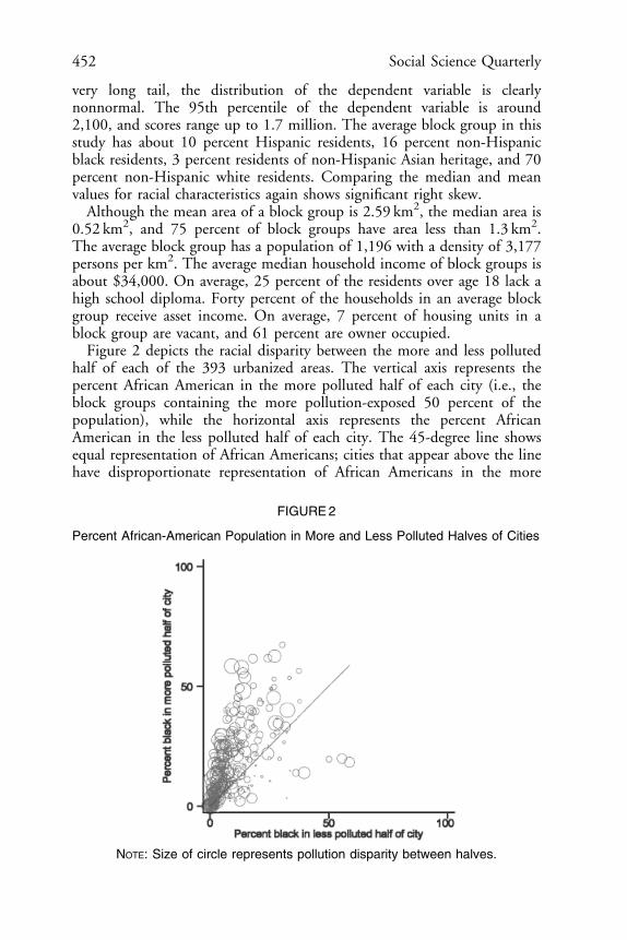
Figure 2 depicts the racial disparity between the more and less pollutedhalf of each of the 393 urbanized areas. The vertical axis represents thepercent African American in the more polluted half of each city (i.e., theblock groups containing the more pollution-exposed 50 percent of thepopulation), while the horizontal axis represents the percent AfricanAmerican in the less polluted half of each city. The 45-degree line showsequal representation of African Americans; cities that appear above the linehave disproportionate representation of African Americans in the more

FIGURE2

Percent African-American Population in More and Less Polluted Halves of Cities

NOTE: Size of circle represents pollution disparity between halves.


polluted half of the city, while cities that fall below the line havedisproportionate representation of African Americans in the less pollutedhalf of the city. The size of each circle represents the pollution disparitybetween the more and less polluted halves of the city. Visual inspectionsuggests that the more polluted halves of most cities are disproportionatelyAfrican American. Equivalent scatter plots (available from the authors) forpercent Hispanic and average income also suggest disproportionate exposurewithin cities. Multivariate analysis reported below support these findings.

Modeling Techniques

The extreme skew of the dependent variable suggests the use of limiteddependent variable estimation rather than OLS. We use the Tobit modeland the linear probability model (LPM). To motivate the censored approachof Tobit, we posit the existence of a latent variable representing theincapacity to avoid pollution; negative values of this latent variable wouldreflect progressively higher levels of capacity to secure environmental quality.But since the observed pollution cannot fall below zero, we observe scores ofessentially zero for many block groups. Because several observations withvery high scores could overwhelm the results, for the Tobit analysis weimpose upper-tail censoring of the dependent variable at 2,300, slightlyabove the 95th percentile, to limit the influence of several very high scoresbut not to discard those block groups altogether. That is, the dependentvariable for the Tobit is both lower and upper censored, with three ranges,that is, below 1, continuous between 1 and 2,300, and larger than 2,300.9

We also apply a dichotomous estimation technique. We estimate theprobabilities that a neighborhood is in the more polluted half and mostpolluted tenth of its city. The quantiles are determined by population; forexample, the most polluted tenth of the city is the set of most polluted blockgroups that contains one-tenth of the population of the urbanized area (notnecessarily in contiguous block groups). Although we lose information inmoving from a continuous to a dichotomous variable, the results of thedichotomous model are readily interpreted. We apply the LPM despite thewell-known problems of induced heteroskedasticity and nonconformingprobabilities because it is consistent even in fixed-effect models.

Regression Results

In this section, we first report results based on the Tobit model withoutand with fixed effects. We then report results based on the dichotomous

9Tobit may be inconsistent in models with fixed effects even when other assumptions aresatisfied, but our fixed-effect Tobit estimates are reliable because the data include many blockgroups within cities. We also estimated the model with OLS, truncating the data at the 99thpercentile, and the results with and without fixed effects are very similar to the Tobit results.


LPM model. Table 2 reports the coefficient estimates and standard errors forthe model specifications estimated with Tobit.

Tobit Model Without Area Fixed Effects

The first two columns of Table 2 report the results of national-levelestimation without urbanized-area effects. In Column 1, where the modelincludes only the race and ethnicity variables, the coefficient on percentAfrican American is positive, indicating that block groups with higherproportions of African Americans tend to have higher RSEI scores, while thecoefficients on percent Hispanic and Asian are both negative, meaning thatblock groups with more of these ethnic groups tend to have lower RSEIscores. When we add income in Column 2, the coefficient on percentAfrican American falls rather sharply but remains positive and materially andstatistically significant. This result implies that the positive relationship

TABLE2

Results for Tobit Estimation, With and Without Area Fixed Effects

Area fixed effects1 2 3 4 5No No 393 UAs 393 UAs 393 UAs

% Hispanic � 2.25 n n � 4.68 n n 3.07 n n 0.96 n n � 0.39 n n

(0.09) (0.09) (0.08) (0.08) (0.10)% African American 2.87 n n 0.24 n n 2.32 n n 0.81 n n 0.23 n n

(0.06) (0.06) (0.04) (0.048) (0.05)% Asian/PacificIslander

� 10.64 n n � 8.26 n n � 0.123 � 0.91 n n � 0.82 n n

(0.25) (0.24) (0.188) (0.19) (0.19)Median householdincome (000)

� 18.4 n n � 10.2 n n � 6.03 n n

(0.3) (0.2) (0.27)Square of income 0.0997n n 0.061 n n 0.038 n n

(0.0023) (0.002) (0.002)Population density(1,000/km2)

� 1.20 n n

(0.23)% Adults without HSdiploma

3.18 n n

(0.11)% Households withasset income

� 0.64 n n

(0.10)% Vacant housing 2.34 n n

(0.17)% Owner-occupiedhousing

0.020(0.061)

R2 0.3% 0.7% 5.5% 5.7% 5.8%

#significant at po0.10; nsignificant at po0.05; n nsignificant at po0.01.

NOTES: Dependent variable is RSEI score: 1,376 observations left censored at or below 1; 6,209observations right censored at or above 2,300. All variables are in units indicated in Table 1.Constant is included in Columns 1 and 2. Standard errors are in parentheses.


observed between the percent of African-American residents and the RSEIscore observed in Column 1 is in part due to the negative correlationbetween percent African-American residents and household income.Likewise, the magnitude of the negative relationship for Hispanics increaseswhen income controls are added, which suggests that Hispanic exposure ishigher because of lower average Hispanic income. However, the magnitudeof the negative relationship between percent Asian and pollution diminishesafter income is included, meaning that Asians are more exposed than theirincomes alone would suggest. Higher median income is strongly associatedwith lower pollution. The quadratic and linear terms imply a concaverelation with the minimum at $92,000, which means that virtually everyblock group lies in the domain where increasing income is associated withdecreasing pollution exposure.

Tobit Model with Area Fixed Effects

The fixed-effect estimates shown in Columns 3 and 4 of Table 2 reveal astriking difference between demographic correlations between cities andcorrelations within cities. Within urbanized areas, the strong positiverelationship between percent African American and pollution score persists.But when base pollution levels are permitted to vary among cities, there is apositive relationship between the percentage of Hispanics in a block groupand the RSEI score. Taken together, results from the models with fixedeffects (Columns 3 and 4) and the corresponding models without fixedeffects (Columns 1 and 2) suggest that Hispanics live in cleaner cities, butthat within the cities where they live, they tend to live ‘‘on the wrong side ofthe environmental tracks’’—that is, in more polluted block groups.

The coefficient on the percent of African Americans remains positive andsignificant in the fixed-effects model. Taken together, the results of themodels without and with fixed effects indicate that African Americans liveboth in more polluted cities in the United States and also in the morepolluted block groups of the cities in which they live. The magnitude of theintra-city effect revealed by the fixed-effect models is stronger for Hispanicsthan for African Americans in Columns 3 and 4. In all the Tobitspecifications, Asians are found to live in less polluted neighborhoods. Theincome coefficients remain stable with the addition of the 393 urbanizedarea fixed effects. The quadratic and linear terms imply that the minimumoccurs at around $80,000; more than 95 percent of block groups are in thedecreasing part of the function.

Visual inspection of a national RSEI-score map and regression analysis,available from the authors, suggest that the racial and ethnic between-cityresults are largely due to the concentration of Hispanics and Asians in theWest and the Southwest, which generally have lower concentrations of heavyindustry and TRI emitters. This analysis also finds that the intercity effect


for African Americans—African Americans tend to live in significantly morepolluted cities than do whites—is due to the concentration of AfricanAmericans in the Rust Belt cities of the Northeast and Midwest.

To elaborate the social characteristics that drive the results, we included anextended list of covariates (Column 5 of Table 2). The coefficient on percentAfrican American is reduced, although the value remains positive and highlysignificant. The sign on percent Hispanic becomes negative, which suggeststhat the Hispanic effect is largely explained by other social characteristics,including education, unearned income, and housing vacancy rate. Thecoefficient on population density is negative, which implies that withinurbanized areas, less densely populated block groups have higher RSEIscores. This finding suggests that planners and public health officials work tolocate polluting facilities in sparsely populated areas, but is also consistentwith the proposition that sparsely populated urban areas have less politicalinfluence. The fraction of vacant housing units is also associatedwith increased pollution; high vacancy is not a correlate of low density(r5 –0.0062) but may reflect neighborhood disempowerment or distress.Block groups with a greater proportion of adults without high schooldiplomas, and those with a lower proportion of households receiving assetincome, tend to be more polluted.

Despite the high fraction of block groups with pollution scores near zero,which could bias OLS results, simple OLS regression yielded results verysimilar to those of Tobit, albeit with slight attenuation in the coefficients.The imposition of the upper censoring, however, had substantial effects onthe results. If the highest values of the RSEI score are included, they drivethe results and generate substantially different regression coefficients.10

LPM Results

In Table 3, we report the probability that a block group is in the mostpolluted fraction of its urbanized area as a function of its socialcharacteristics. The results are based on a fixed-effects linear probabilitymodel, and thus are most comparable to Columns 3 through 5 of Table 2.In the first three columns, we examine the probability that a block group isamong the more polluted half of its city. The estimated coefficients in theLPM can be interpreted as percentage point changes. For example, inColumn 1 of Table 3 we find that a block group that is 100 percentHispanic has a probability 51 percentage points greater of being in the morepolluted half of the city compared to an otherwise identical block group that

10The censoring value makes little difference. We tested censoring at centiles 90, 95, 99,and 99.5 and found very similar Tobit results for all upper-censoring points. The blockgroups with the very highest scores, which have median incomes close to the overall medianand are more white than is the average block group, exert substantial leverage.


TABLE3

ResultsforLPM

EstimationwithAreaFixedEffects

12

34

56

Most

polluted:::ofUA

Half

Half

Half

10th

10th

10th

%Hispanic

0.517nn

0.228nn

0.061

nn

0.194

nn

0.094nn

�0.008

(0.009)

(0.010)

(0.012)

(0.006)

(0.006)

(0.008)

%AfricanAmeric

an

0.337nn

0.138nn

0.086

nn

0.083

nn

0.014nn

�0.033

nn

(0.005)

(0.006)

(0.006)

(0.003)

(0.004)

(0.004)

%Asian/PacificIslander

0.103nn

0.000

�0.040#

�0.037

nn

�0.073nn

�0.050

nn

(0.022)

(0.022)

(0.022)

(0.015)

(0.015)

(0.015)

Medianhousehold

income(000)

�0.0121

nn

�0.0082

nn

�0.0043

nn

�0.0011

nn

(0.0002)

(0.0003)

(0.0001)

(0.0002)

Square

ofincome

0.000061

nn

0.000040

nn

0.0000222nn

0.0000052

nn

(0.000002)

(0.000002)

(0.0000013)

(0.0000015)

Populatio

ndensity

(1,000/km

2)

0.0004

nn

�0.0003

nn

(0.0003)

(0.0002)

%Adults

with

outHSdiploma

0.325

nn

0.245

nn

(0.014)

(0.009)

%Householdswith

assetincome

�0.027

n�0.083

n

(0.012)

(0.008)

%Vacanthousing

0.06

nn

0.080

nn

(0.02)

(0.013)

%Owner-occupiedhousing

�0.0006

�0.0044

(0.0072)

(0.0047)

R2(with

in)

5.3%

8.6%

9.2%

1.2%

2.2%

3.3%

#significantatpo0.10;

nsignificantatpo0.05;

nnsignificantatpo0.01.

NOTES:Dependentvaria

ble

isdichotomous,

with

1indicatin

ginclusionin

themore

pollutedsegmentofthecity.Allvaria

blesare

inunits

indicatedin

Table

1.

Coefficients

exp

ress

thepercentagepointchangein

probability

ofexp

osu

reperunitchangein

theexp

lanatory

varia

ble.Standard

errors

are

inparentheses.


is 100 percent white non-Hispanic. The results indicate that block groupsthat are a higher proportion Hispanic, African American, or Asian are allmore likely to be in the more polluted half of the urbanized area, althoughthe Asian effect disappears when controls for income are added. We also findthat over most of the observed range of incomes, income is negativelycorrelated with the probability of being in the more polluted half of the city,and the minimum of the income-pollution gradient occurs at aneighborhood income of $99,000. At the median, a $10,000 increase inincome is associated with a seven percentage point decrease in theprobability of being in the more polluted half of the city. In the elaboration(Column 3), we find, as in the Tobit model, that block groups with a higherfraction of adults who did not graduate from high school are substantiallymore likely to be in the more exposed half and that asset income isassociated with less pollution exposure.

When we turn to the most polluted 10th of cities, the explanatory power ofthe model drops, but most of the results persist (Columns 4 through 6 ofTable 3). In Column 4, which shows results for a model that includes onlythe race and ethnicity variables, we find that Hispanics and AfricanAmericans are substantially more likely than non-Hispanic whites to live inthe most polluted 10th of cities, and Asians are less likely to live in the mostpolluted 10th. When median household income is included in theregression, the race and ethnicity effects decline but remain positive andsignificant. When we include the full set of neighborhood covariates, thesigns on the coefficients for percent Hispanic and percent African Americanactually reverse, although the size of the coefficients is small. This resultsuggests that for inclusion in the most polluted portions of the city, theother social indicators explain the correlations between pollution andHispanic and African American. We find strong negative associationsbetween inclusion in the most polluted 10th and both population densityand asset income; we find strong positive relationships between presence inthe most polluted 10th and both vacant units and adults with less than highschool education. Higher neighborhood income implies a steadily decliningprobability of membership in the most polluted 10th.11

The models explain a small proportion of the variation in the RSEI score.Without fixed effects, the pseudo-R2 for the Tobit regressions in Table 2 arebelow 0.01. When we estimate the same models using OLS, the R2 in themodels without fixed effects reach only 0.12 for the models with the full setof explanatory variables. Even when we estimate the models with 393urbanized area fixed effects, the pseudo-R2 of the Tobits climbs only toaround 0.06. Although R2 is a poor measure of fit for the LPM, the within-city R2 for the fixed-effect linear probability models ranges from 0.01 for the

11We also examined the correlates of the worst quarter and of centiles 75 through 90, andfound results that were generally intermediate between those for the worst 10th and the worsehalf.


sparest specification of the regression for the most polluted 10th, to 0.09 forthe richest specification of the regression for the more polluted half.

In the few studies of environmental inequality that report R2, the per-centage of variation explained exceeds that of our model. We experimentedwith adding variables used by authors whose models had higher R2 andfound that the additional variables do not substantially raise the R2 of ourmodel. Aggregated analyses are likely to have upward-biased R2 because ofthe ecological fallacy. Our highly disaggregated analysis reduces its effect.Despite a low proportion of explained variation, we find statisticallysignificant correlations between demographic variables and pollution, asevidenced by the high t-statistics in the multivariate results.

Discussion and Conclusions

Previous environmental justice research has generally failed to address thedemographics of pollution in terms of toxicity and exposure, focusinginstead on proximity to pollution sources or on the mass of pollutantsreleased. Many previous studies use large units of spatial resolution, andmost national studies control for regional variation, if at all, only byestimating correlations separately for a small number of regions in thecountry or separately for densely and sparsely populated regions.

This article addresses these issues by using data from the EPA’s RSEIModel. Our results indicate that in the urban United States as a whole,block groups with more African Americans have higher levels of exposure totoxic pollution from TRI facilities, while block groups with more Hispanicsand Asians/Pacific Islanders have lower levels. When we control fordifferences between cities, however, we find that within cities, Hispanics, aswell as African Americans, tend to live in more polluted neighborhoods. Innational comparisons, this disparity is offset for Hispanics by the fact thatthey tend to live in cities with relatively low levels of industrial toxics.African Americans, by contrast, tend to live in more polluted cities as well asin the more polluted neighborhoods within cities.

There are several important caveats regarding the data underlying thisanalysis. First, our dependent variable represents only a subset of pollutantsthat people face. Mobile and small point sources, such as automobiles anddry cleaners, are excluded. The data also omit exposure via other media, suchas water pollution and nonresidential, for example, workplace, exposure.Second, the measure of toxicity does not include possible synergistic effectsof multiple pollutants. Third, although the RSEI Model incorporates muchsite-specific data, the dependent variable relies on modeling and somegeneralizations.

Our methodology also warrants several caveats. A cross-sectional analysiscannot elucidate causal relationships between demographics and pollution.The correlations between the demographic variables and RSEI scores could


be caused by various underlying factors. For instance, even when incomes aresimilar, African Americans or Hispanics may have lower average wealth thando whites, which would constrain housing choices. African Americans orHispanics also may tend to have less access to information about the healtheffects of pollution. Or there may be racism in housing or credit markets, orin the siting of industrial facilities. This study cannot ascertain whichprocesses underlie the results. We note, however, that the strong effect of raceand ethnicity, controlling for income, suggest that voluntary move in spurredby low income is not a plausible explanation for differences in exposure.

Two previous national studies account both for relative toxicity and foratmospheric dispersion. Their results are only partially comparable due todifferences in methodology but are generally consistent with respect to thecoefficients on race and ethnicity variables. Brooks and Sethi (1997) report apositive correlation between the percent of African Americans in a zip codeand their index of pollution. Bouwes, Hassur, and Shapiro (2001) report apositive correlation between their index of pollution and both the percent ofAfrican Americans and the percent of Hispanics.12

This study offers three key insights to inform future research and policy.First, different minority groups should be included separately in econo-metric analysis rather than lumped together as ‘‘all nonwhite’’ residents.Second, national environmental justice studies should account for variationsin base levels of pollution in order to avoid collapsing variation within citiesand variation among cities into a single coefficient. Third, for analyzingexposure (though not necessarily proximity to point sources), the spatial unitof analysis should be as small as possible because larger units can obscureheterogeneity.

What are the conclusions for environmental justice policy? Our resultssupport past findings that pollution burdens fall disproportionately onAfrican Americans and poor people throughout the United States—and onHispanics within regions. Our results also suggest that local policymakersbear special responsibility to address disparate exposure. The results forAfrican Americans imply that environmental justice should remain a priorityfor national as well as regional environmental policy. In addition, the resultshighlight the value of the EPA’s RSEI data for environmental justiceanalyses. The fine geographic resolution and well-developed dependentvariable make these data exceptionally well suited to analyze the demo-graphics of pollution.

12Although Bouwes, Hassur, and Shapiro (2001) also use RSEI data to generate adependent variable, the positive sign on the Hispanic variable differs from our result in themodel without fixed effects. Three methodological differences may account for the difference.Their measure of pollution is weighted by population, so that more populated areas havehigher values of pollution even if the unweighted pollution level is the same; they use onlyobservations for which the value of the RSEI score is greater than zero; and the unit of theiranalysis is the square-kilometer cell rather than the Census block group.


REFERENCES

Anderton, D. L., A. B. Anderson, P. H. Rossi, J. M. Oakes, M. R. Fraser, E. W. Weber, andE. J. Calabrese. 1994. ‘‘Hazardous Waste Facilities: ‘Environmental Equity’ Issues inMetropolitan Areas.’’ Evaluation Review 18(2):123–40.

Arora, S., and T. N. Cason. 1999. ‘‘Do Community Characteristics Influence EnvironmentalOutcomes? Evidence from the Toxics Release Inventory.’’ Southern Economic Journal65(4):691–716.

Been, V., and F. Gupta. 1997. ‘‘Coming to the Nuisance or Going to the Barrios? ALongitudinal Analysis of Environmental Justice Claims.’’ Ecology Law Quarterly 24(1):1–56.

Boer, J. T., M. Pastor, J. L. Sadd, and L. D. Snyder. 1997. ‘‘Is There Environmental Racism?The Demographics of Hazardous Waste in Los Angeles County.’’ Social Science Quarterly78(4):793–810.

Bouwes, N. W., and S. M. Hassur. 1997. Toxics Release Inventory Relative Risk-Based Environmental Indicators Methodology. Washington, DC: U.S. EPA Office ofPollution Prevention and Toxics. Available at hhttp://www.epa.gov/oppt/rsei/docs/meth-od97.pdf i.

———. 1998. Groundtruthing of the Air Pathway Component of OPPT’s Risk-Screening Environmental Indicators Model (Draft). Washington, DC: U.S. EPA Office ofPollution Prevention and Toxics. Available at hhttp://www.epa.gov/oppt/rsei/docs/ground98.pdfi.———. 1999. Estimates of Stack Heights and Exit Gas Velocities for TRI Facilities in OPPT’sRisk-Screening Environmental Indicators Model. Washington, DC: U.S. EPA Office ofPollution Prevention and Toxics. Available at hhttp://www.epa.gov/oppt/rsei/docs/stacks99.pdf i.

———. 2002. User’s Manual for RSEI Version 2.0 Beta 2.0. Washington, DC: U.S. EPAOffice of Pollution Prevention and Toxics. Available at hhttp://www.epa.gov/oppt/rsei/docs/users_manual.pdf i.Bouwes, N. W., S. M. Hassur, and M. D. Shapiro. 2001. Empowerment Through Risk-RelatedInformation: EPA’s Risk-Screening Environmental Indicators Project. Working Paper DPE-01-06. Amherst, MA: Political Economy Research Institute.

Bowen, W. M., M. J. Salling, K. E. Haynes, and E. J. Cyran. 1995. ‘‘Toward EnvironmentalJustice: Spatial Equity in Ohio and Cleveland.’’ Annals of the Association of AmericanGeographers 85(4):641–63.

Brooks, N., and R. Sethi. 1997. ‘‘The Distribution of Pollution: Community Characteristicsand Exposure to Air Toxics.’’ Journal of Environmental Economics and Management 32:233–50.

Chakraborty, J., and M. P. Armstrong. 1997. ‘‘Exploring the Use of Buffer Analysis for theIdentification of Impacted Areas in Environmental Equity Assessment.’’ Cartography andGeographic Information Systems 24(3):145–57.

Glickman, T. S., and R. Hersh. 1995. Evaluating Environmental Equity: The Impacts ofIndustrial Hazards on Selected Social Groups in Allegheny County, Pennsylvania. DiscussionPaper 95–13. Washington, DC: Resources for the Future.

Hird, J. A., and M. Reese. 1998. ‘‘The Distribution of Environmental Quality: An EmpiricalAnalysis.’’ Social Science Quarterly 79(4):693–716.

Kriesel, W., T. J. Centner, and A. G. Keeler. 1996. ‘‘Neighborhood Exposure to ToxicReleases: Are There Racial Inequities?’’ Growth and Change 27:479–99.


McMaster, R., H. Leitner, and E. Sheppard. 1997. ‘‘GIS-Based Environmental Equity andRisk Assessment: Methodological Problems and Prospects.’’ Cartography and GeographicInformation Systems 24(3):172–89.

Mohai, P. 1995. ‘‘The Demographics of Dumping Revisited: Examining the Impact ofAlternate Methodologies in Environmental Justice Research.’’ Virginia Environmental LawJournal 14:615–53.

Mohai, P., and B. I. Bryant. 1992. ‘‘Environmental Racism: Reviewing the Evidence.’’ InRace and the Incidence of Environmental Hazards: A Time for Discourse. Boulder, CO:Westview Press.

Oakes, J. M. 1997. ‘‘The Location of Hazardous Waste Facilities.’’ Ph.D. Dissertation.Amherst, MA: University of Massachusetts Amherst.

Pastor, M. 2001. Building Social Capital to Protect Natural Capital: The Quest forEnvironmental Justice. Working Paper DPE-01–02. Amherst, MA: Political EconomyResearch Institute.

Rabin, Y. 1989. ‘‘Expulsive Zoning and the Legacy of Euclid.’’ Pp. 101–21 in C. M. Haarand J. S. Kayden, eds., Zoning and the American Dream: Promises Still to Keep. Chicago, IL:Planners Press and American Planning Association in association with Lincoln Institute ofLand Policy.

Szasz, A., and M. Meuser. 1997. ‘‘Environmental Inequalities: Literature Review andProposals for New Directions in Research and Theory.’’ Current Sociology 45(3):99–120.

United Church of Christ. Commission for Racial Justice. 1987. Toxic Wastes and Race in theUnited States: A National Report on the Racial and Socioeconomic Characteristics ofCommunities with Hazardous Waste Sites. New York: United Church of Christ.

U.S. Department of Commerce. 1992. 1990 Census of Population and Housing: STF 3 onCD-ROM. Washington, DC: Economics and Statistics Administration, Bureau of theCensus.

———. 1994. Geographic Areas Reference Manual. Washington, DC: Economics andStatistics Administration, Bureau of the Census. Available at hhttp://www.census.gov/geo/www/garm.htmli.

U.S. Environmental Protection Agency. 1995. User’s Guide for the Industrial Source Complex(ISC3) Dispersion Models, Volume II—Description of Model Algorithms. Research Triangle Park,NC: U.S. EPA. Available at hhttp://www.epa.gov/scram001/userg/regmod/isc3v2.pdf i.

———. 1999. Fact Sheet: Risk-Screening Environmental Indicators. Washington, DC: Officeof Pollution Prevention and Toxics. Available at hhttp://www.epa.gov/oppt/rsei/docs/factsheet_v2.pdf i.———. 2000. Summary of 1998 Toxics Release Inventory Data. Available at hhttp://www.epa.gov/tri/tridata/tri98/data/1998datasumm.pdf i.


Documents

Who Lives on the Wrong Side of the Environmental … · 2016-11-12 · highlight the importance of controlling for interregional variation in pollution levels ... regional variations