Who pays the price when housing bubbles burst? Evidence from the

Who pays the price when housing bubbles burst?

Evidence from the American Community Survey

Cynthia Bansak St. Lawrence University

Martha A. Starr

American University

January 2010

Abstract There has been much debate in recent years about whether the Federal Reserve should have taken action against the housing-price bubble as it was forming. One argument in favor of using monetary policy to offset asset-price bubbles is that it may be impossible after the bubble bursts to ease policy hard enough or fast enough to offset a strong contraction. While the fall in housing prices since 2006 has clearly increased unemployment and depressed growth, much less is known about how the costs have been distributed across households of different means. This paper uses data from the Census Bureau’s annual American Community Survey (ACS) to examine this question. We first lay out the mechanisms via which a housing-market bust would be expected to affect households, in terms of incomes, employment, assets, and ability to service debt. We then use the ACS data to analyze how the house-price bust has affected households with different characteristics, differentiating between communities in which home prices did and did not boom and bust. Our results suggest that costs of the bubble have tended to fall on households less able to endure periods of financial distress. This lends further support to the argument that monetary policy oriented to social welfare should tackle bubbles ex ante rather than ex post.

________________________________________________________________________________

Please address correspondence to: Martha A. Starr, Dept. of Economics, American University, 4400 Mass. Ave. NW, Washington, DC 20016. Tel: 202-885-3747. Email: [email protected]. We are grateful to Karl Case and participants in an ASE session on “Socio-distributional effects of the financial crisis” at the 2010 ASSA meetings in Atlanta for their valuable comments on an earlier version of this paper.

- 2 -

Introduction

There has been much debate in recent years about whether the Federal Reserve should have taken

action against the housing-price bubble as it was forming. As home prices rose, the Fed’s position was

that it was difficult to know whether a bubble was developing, and that monetary policy could always

be eased if declining prices posed risks to continued expansion.1 As much as it is now widely recognized

that this was not a prudent position,2 there remains little consensus as to whether monetary policy

should incorporate any systematic concern with asset-price bubbles, above and beyond what is implied

by its core concerns with inflation and unemployment. Thus, for example, pro-cyclical adjustments in

capital requirements could be used to keep asset values from drifting out of line with their underlying

values (Yellen 2009, Evans 2009).

An important issue in this respect concerns who pays the price when an asset-price bubble bursts.

Conceivably it may be of little social benefit to offset a potential bubble which, if it later burst, would

impose costs on a relatively narrow and well-off segment of the population. Thus, for example, the

high-tech stock bubble of the late 1990s affected shareholders and employees of high-tech companies,

who were largely highly skilled and well-educated. In contrast, the housing-price bubble that burst in

2006 and precipitated an aggregate downturn imposed costs on a wide swath of the households and

businesses -– although we know little as yet about how these were distributed. Characterizing the

distributional effects of housing-price booms and busts is important in view of recent theoretical work

on business cycles, which suggests that allowing for heterogeneities may significantly alter estimated

welfare effects of aggregate fluctuations.3

To date, there has been little systematic research on the distribution of benefits and costs of housing-

price bubbles. In an early paper, Case and Cook (1988) found that rising home prices increased the

consumption opportunities of existing homeowners while decreasing those of renters and prospective

homebuyers; much research since then confirms this finding (e.g. Gyourko and Tracy 1999). Mayer

(1993) found that prices of lower-end housing tend to increase more rapidly during housing booms than

those of higher-end housing, but that the volatility of higher-end housing is greater. Quigley and

Raphael (2001) identify high housing costs as a significant determinant of variations in homelessness

across areas, suggesting that housing-price bubbles contribute to problems of access to housing for very

low income people. Work by Baker and Rosnick (2008) using the Survey of Consumer Finances suggests

1 See, e.g. Bernanke (2002), Rudebusch (2005), Lansing (2005), Kohn (2008), Mishkin (2008). 2 In the words of San Francisco Federal Reserve President Janet Yellen (2009), it is now “patently obvious … that not dealing with certain kinds of bubbles before they get big can have grave consequences.” 3 Notably, see Krusell, Mukoyama, Sahin, and Smith (2009), and also Barlevy (2004) and Imrohoroglu (2008).

- 3 -

that the current drop in housing prices is particularly detrimental for households in the middle of the

wealth distribution, given the importance of home equity in their portfolios. A shortcoming of existing

research is that it tends to focus on housing-related issues without considering aggregate implications.

Notably, rising house prices per se may be detrimental for low-to-moderate income households, but if

they stimulate residential investment and/or boost consumer spending due to wealth effects, they may

also improve prospects for income and employment. Thus, understanding how housing-price bubbles

affect income and employment patterns, as well as housing-related outcomes, is beneficial for gauging

how their costs and benefits are distributed across groups within the population.

This paper uses data from the Census Bureau’s annual American Community Survey (ACS) to examine

this question. Each year, the ACS collects social, demographic, housing and economic information from

a nationally representative sample of 3 million U.S. households. Presently data are available for 2005-

2008, enabling us to examine how the bursting of the housing price bubble after 2006 has affected

households with varying characteristics. The next section of the paper lays out three mechanisms via

which housing-market booms and busts affect the broader economy and different types of households

within it: namely, wealth-effects on spending, swings in residential investment, and problems of

financial distress. We then use data from the 2005-2008 waves of the ACS to analyze how the housing-

price bust has affected households with different characteristics, differentiating between communities

in which home prices did and did not boom and bust. Our results suggest that costs of the bubble have

tended to fall on households less able to endure periods of financial distress. This lends further support

to the argument that monetary policy oriented to social welfare should tackle bubbles ex ante rather

than ex post.

Conceptual issues and existing research

Case and Quigley (2008) identify three mechanisms via which the unwinding of a housing boom would

be expected to affect the broader economy. The first is the wealth effect on spending, whereby a

decline in home prices reduces the net worth of homeowners, causing them to reduce their spending to

reflect the lower value of their total wealth. Research by Case, Quigley and Shiller (2005), Carroll,

Otsuka and Slacalek (2006), and Bostic, Gabriel and Painter (2009) suggests that, ceteris paribus, a $1

increase in housing wealth would boost spending by 4-8 cents, with the effect phasing in over the next

2 or 3 years. Estimates of the housing-wealth effect are stronger than those for stock-market wealth,

which range between 2-5 cents per dollar, due to the greater prevalence of homeownership versus

stockownership and a higher marginal propensity to consume among homeowners versus stockholders.4

At the same time, higher home prices also boost the housing costs of renters, cutting into their ability

4 It is also likely that the housing-wealth effect has strengthened over time due to greater opportunities to cash out gains in home equity via mortgage refinancing (Muellbauer 2008).

- 4 -

to spend on other goods.5 Nonetheless, because 66% of households are owner-occupied and home-

owning households account for 77% of total consumer spending, the housing-wealth effect is estimated

to be positive and strong on balance.6

Via this mechanism, the bursting of the housing-price bubble would be expected to slow growth of

consumer spending and exert a drag on output, incomes and employment over the next few years. To

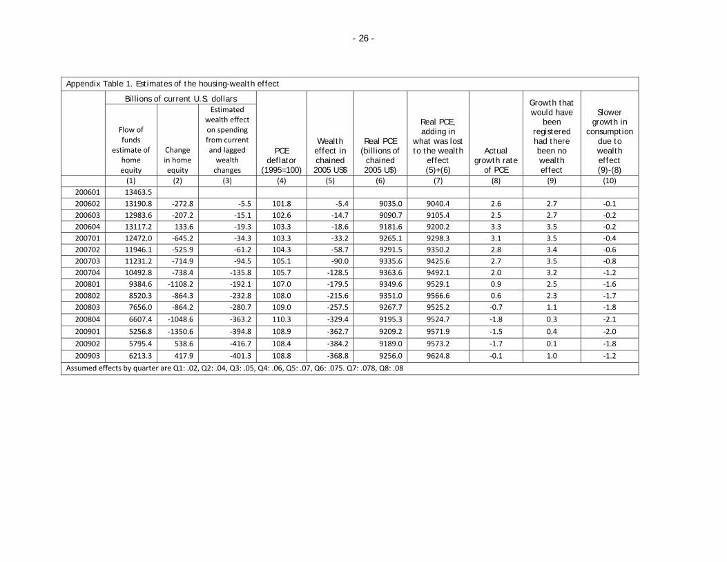
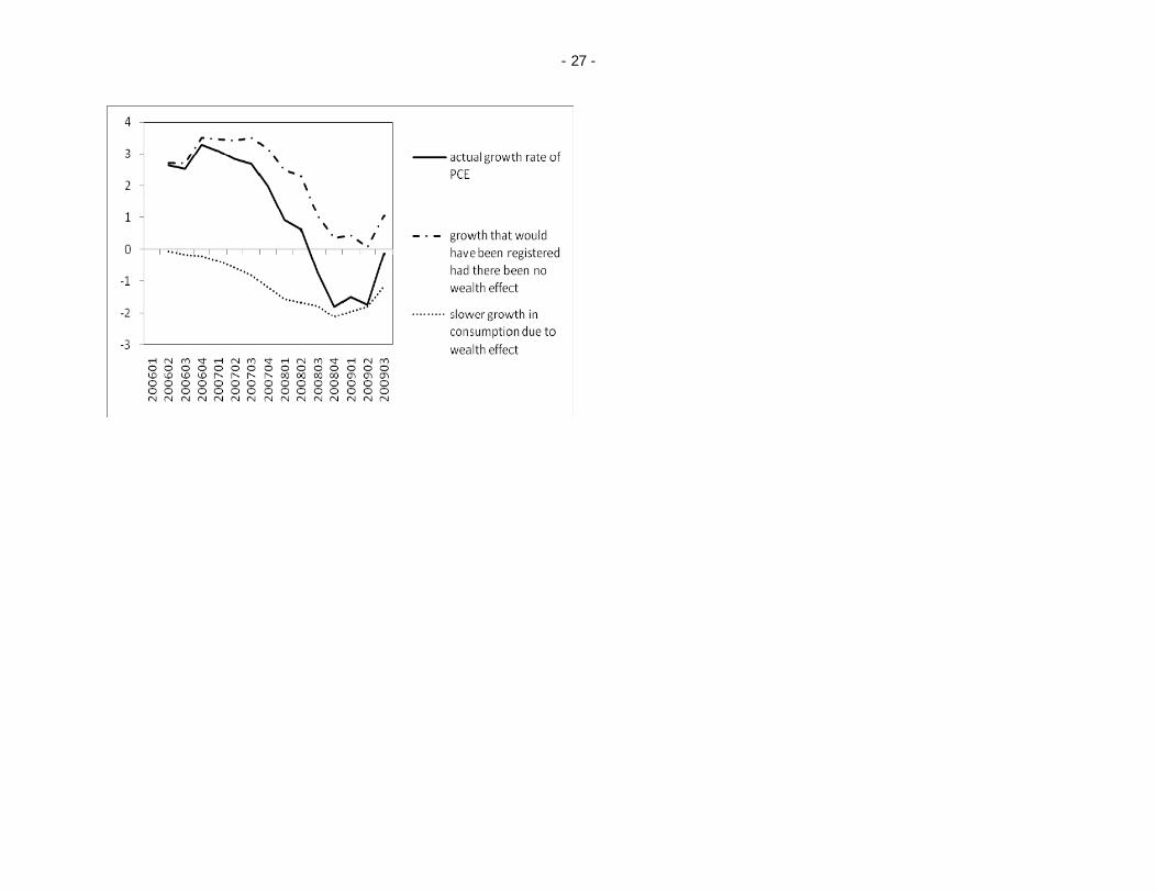
provide a sense of the magnitude of the effect, we can use Carroll, Otsuka and Slacalek’s (2006)

estimates of a same-quarter wealth effect of 2 cents per dollar that increases to 8 cents per dollar

after two years and data on the declining value of housing wealth from the Federal Reserve’s Flow of

Funds (see Appendix Table 1). Based on the extent of the decline in housing wealth and its time

profile, we estimate that it had reduced real consumption growth by 1/2 of a percentage point by

2006:Q4, 1-1/2 percentage points by 2007:Q4, and 2 percentage points by 2008:Q4.7 How this would

affect employment and incomes among people of differing characteristics is not clear from existing

research. To the extent that the reduction in spending follows the usual pattern in cyclical downturns,

it would be expected to disproportionally affect spending on durable goods, as well as spending on

discretionary goods and services (e.g. recreational travel, restaurant meals, fashion clothing).8 It would

also be expected to lead to higher unemployment, with people having less education and/or who are

black or Hispanic experiencing the largest increases in unemployment rates (Blank 1989, Hoynes 2000,

Spriggs and Williams 2000). Geographically, adverse wealth-effects on spending may tend to be

somewhat larger in areas that experienced house-price bubbles due to declining demand for locally-

produced goods and services. On the other hand, the decline in housing prices would be expected to

reduce upward pressures on rents in areas that had had bubbles, making housing more affordable for

renters.

The second mechanism via which an unwinding housing boom would affect the broader economy is

declining residential investment. Periods of unusual run-ups in prices tend to be associated with booms

in residential investment, which in turn raise incomes and employment -- both because of the

construction activity itself and because of relatively high multiplier effects associated with residential

5 Earlier research by Sheiner (1995) and Englehart (1996) found some evidence that higher home prices could reduce spending by prospective homeowners, due to the need to save for a down-payment. This offset has likely become less important in the past decade, as down-payment requirements slipped. 6 Authors’ computations from the 2008 Consumer Expenditure Survey. 7 Note that Carroll, Otsuka and Slacalek’s estimates of the wealth effect are on the high side. Case and Quigley (2008) argue that there is an asymmetry in the housing-wealth effect, such that a given decline in housing wealth may reduce spending by less than a comparable increase boosts it. 8 Using data from the Consumer Expenditure Survey, Bostic, Gabriel and Painter (2009) find that changes in housing wealth especially increase spending on non-durable goods. Note that, whereas their study aimed to characterize effects of wealth on consumption, ours is in its effects on production and employment; given the differential importance of imports across categories of goods, it is not clear that higher spending on nondurable goods necessarily means higher domestic production of them.

- 5 -

investment (Fair 2004, Case and Quigley 2008). Thus, Case and Quigley (2008) expected a marked

decline in the pace of new home construction to represent the largest effect of the housing-price bust

on the broader economy, and indeed data from the National Income and Product Accounts show that it

was a major factor pulling down growth of real GDP growth in 2007 and 2008.9

Whether we should expect declining construction investment and employment to be worst in areas that

had the most sizable housing-price bubbles is not clear from existing research. Several previous studies

suggest that housing-price bubbles are most likely to build in areas where land is scarce, so that

increased demand pushes up price rather than eliciting increased supply of new homes (Glaeser,

Gyourko, and Saiz 2008). In this case, it is possible that adverse effects on employment and incomes

may not be concentrated in areas that had the worst housing-price bubbles, as these may not have

experienced particularly strong booms in investment (Goodman, and Thibodeau 2008). In terms of what

types of people would be most affected by a construction slump, it is important to note that the

construction industry employs people with varied levels of education, training, skill, and experience --

ranging from construction laborers (12-13% of the construction work force in 2005), to skilled craftsman

like carpenters, electricians and masons (40%), to office and administrative support staff (14%), to

construction managers (who earned $91,000 per year on average and made up 7.5% of the work force in

2005).10 But to the extent that the least skilled workers and/or minorities are the first to be laid off

when construction business turns down, declining residential investment may also have regressive

effects on incomes and employment. We can also expect declining construction to adversely affect

production and distribution of building materials and supplies, so that its effects may not be confined

to markets that had had construction booms.

The third channel via which a decline in housing prices affects the broader economy is financial.

Because home sales tend to boom during housing-price bubbles, people shift out of jobs in other

sectors and occupations and into jobs in real estate and finance (Hsieh and Moretti 2003). As prices fall

and sales drop off, incomes and employment in real estate and finance decline; given that jobs in

these fields require relatively high levels of education and/or training, job loss here may affect people

in the middle-to-upper part of the income distribution. Additionally, because returns to

homeownership seem so high during bubbles, and costs of waiting to buy rise, households that might

otherwise rent may instead buy via leverage, taking on debt payments that are high relative to their

incomes. Especially for households who bought late in the boom, a subsequent price drop can leave

them holding an asset worth less than the debt associated with it, with little free cash-flow to spare.

9 Whereas residential investment had been adding ½ a percentage point to growth of real GDP in 2003 and 2004, in 2007 and 2008 its contraction pulled GDP growth down by more than 1 percentage point. Figures from the Bureau of Economic Analysis, National Income and Product Accounts Table 1.5.2, as of December 15, 200. 10 Data from the Bureau of Labor Statistics’ Occupational Employment Statistics, 2005-2008.

- 6 -

This problem was much exacerbated by growth of subprime lending in the past 10-15 years, where the

availability of low- or no-downpayment loans increased the likelihood of going ‘underwater’ when

housing prices turned down, and mortgage payments on a non-negligible share of subprime loans were

re-setting to higher levels just as housing prices peaked (Gramlich 2007). Thus, rather than being able

to sell their homes to pay off their mortgages, homeowners instead suspended payments and/or

defaulted on their loans. We know from financial data that defaults and foreclosures have increased

significantly since 2007, especially in markets where subprime lending had grown most robustly; we

also know that subprime lending tended to grow most rapidly in areas that had relatively large black

and Hispanic populations (Mayer and Pence 2008). Still, the evidence is less than clear on what types of

households have had to exit from financially unsustainable homeownership arrangements: because the

financial data contain little information on household characteristics, we know only generally what

sorts of borrowers have been caught in this sort of pinch.

Data Data for this study come from the U.S. Census Bureau’s American Community Survey, an annual cross-

section survey which collects social, demographic, housing and economic information from a large

sample of U.S. households. The survey is intended to measure changes between the decennial censuses

and uses a questionnaire similar to its former ‘long form’. As with the census, filling it out and

returning it is required by law. About 250,000 households per month receive the questionnaire in the

mail, yielding a sample size of about 3 million households per year (a 1 in 40 sample).11 The ACS sample

has been broadly representative geographically since 2005, with data presently available for the four

waves between 2005 and 2008.12 However, because relatively small areas have relatively small

numbers of respondents, estimates of changes over time for such areas, especially for subsets of

households within them, move a good deal due to sampling error. Thus, we confine our analysis to the

167 metropolitan statistical areas (MSAs) that had populations of 250,000 or more in the 2005-08

period. These contain about 220 million people, or about three-quarters of the U.S. population.13

To measure how the housing-market bust has affected households with different characteristics, we

categorize metropolitan areas into those which experienced a boom and bust in housing prices, and

those which did not. For this purpose, we use the quarterly all-transaction house-price indexes from

the Federal Housing Finance Agency (FHFA), which are weighted, repeat-sales indexes computed for

11 The ACS makes numerous efforts to contact respondents who do not initially reply, resulting in eventual response rates of 97-98%. 12 In 2001-2004, the ACS sample included 800,000 households and was intended to represent areas with populations of 1 million or more. In 2005, the sample size was increased to 3 million households, with the intention of representing areas with populations of 65,000 or more. 13 The analysis also excludes data for Puerto Rico.

- 7 -

single-family properties having a mortgage purchased by Freddie Mac or Fannie Mae. While the FHFA

data have certain disadvantages relative to the S&P/Case-Shiller home-price indexes, the former are

available for all of the MSAs in our analysis while the latter are not. To identify MSAs that experienced

housing-price bubbles that burst, we use two definitions based on the extent of the increase in the

FHFA price index between 1995:Q1 and the peak value shown in the data, and the extent of the

decline in the price index (if any) between the peak and 2008:Q4. In the first ‘broader’ definition, an

MSA is considered to have had a bubble if prices increased by at least 125% after 1995 and decreased

from the peak by least 10% by 2008:Q4. In second ‘narrow’ definition, the price had to have risen by

150% or more after 1995, and decreased from the peak by 25% or more by 2008:Q4.14

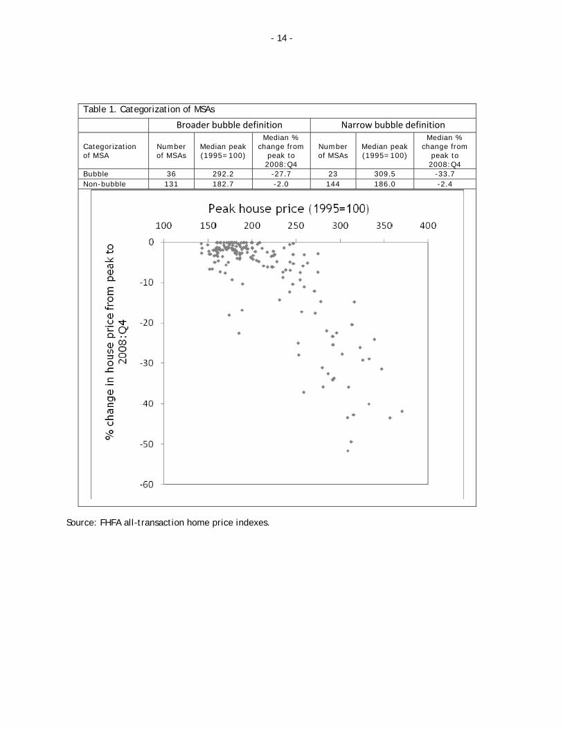
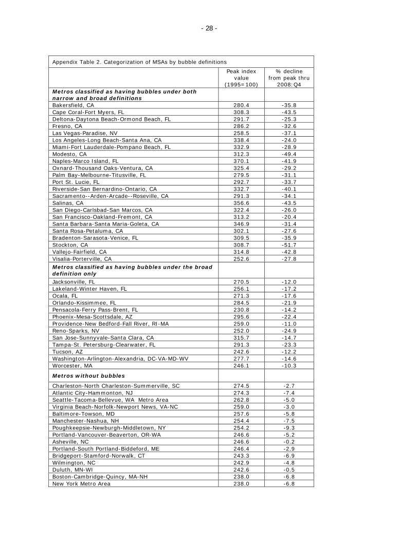
As shown in Table 1, 36 of the 167 MSAs experienced a burst bubble under the broader definition, while

23 had a burst bubble of the narrow type.15 MSAs meeting the narrow definition are all found in

California, Florida, and Nevada; MSAs added in under the broader definition are also found in these

states, as well as Arizona, Massachusetts, and the Washington, DC, metropolitan area (see Appendix

Table 2 for the list). There is of course no assurance that our definitions capture the concept of a

bubble as a period when market prices diverged significantly from prices implied by the underlying

value of housing services (see e.g. Himmelberg, Mayer, and Sinai, 2005, for discussion). But given the

amplitudes of the upswings and downswings in the data, we expect that our definition does a

reasonably good job of identifying metropolitan areas where a bubble in this sense occurred.

In what follows, we compare changes in various measures of housing, incomes, employment, inequality

and poverty across bubble and non-bubble markets. To understand how declining home prices have

affected households with varying characteristics, we use education as a proxy for permanent income,

differentiating between households where the householder had not completed a high school diploma,

had completed a high school diploma but not a college degree, or had completed a college degree.16

We also analyze differences across households by race/ethnicity, given their well-known correlations

with economic outcomes and opportunities. In particular, we differentiate between households where

the householder is white and does not self-identify as Hispanic; those where the householder self-

14 Appendix Figure 1 shows the clear negative correlation between the extent of the run-up in home prices after 1995 and the extent of decline thereafter. Note that, for the 11 largest MSAs, the FHFA provides data for metropolitan divisions within the MSA rather than the MSA itself. In these cases, we computed price changes for the MSA as population-weighted averages of changes for the metropolitan divisions. Note that, in any event, all divisions within a given MSA had the same categorization in 9 of the 11 cases. 15 See the Appendix for details. 16 In the Census definition, the ‘householder’ is the person (or one of the persons) in whose name the housing unit is owned or rented. If a married couple owns the home jointly, either spouse may be the householder. People who undertook some college studies without completing a degree are included with high-school graduates.

- 8 -

identifies as Hispanic; and those who classify their race as black.17 Note that these categories are not

mutually exclusive as people of Hispanic origin may be of any race.

The present version of the paper presents a descriptive analysis of MSA-level data. Thus, for example,

for given a given measure xit related to a housing, income, or employment outcome, where i is the

metropolitan area and t is the survey wave, we calculate changes in the mean and median values of xit

among ‘bubble’ and other metros, and test whether the difference between the two is significant.18 To

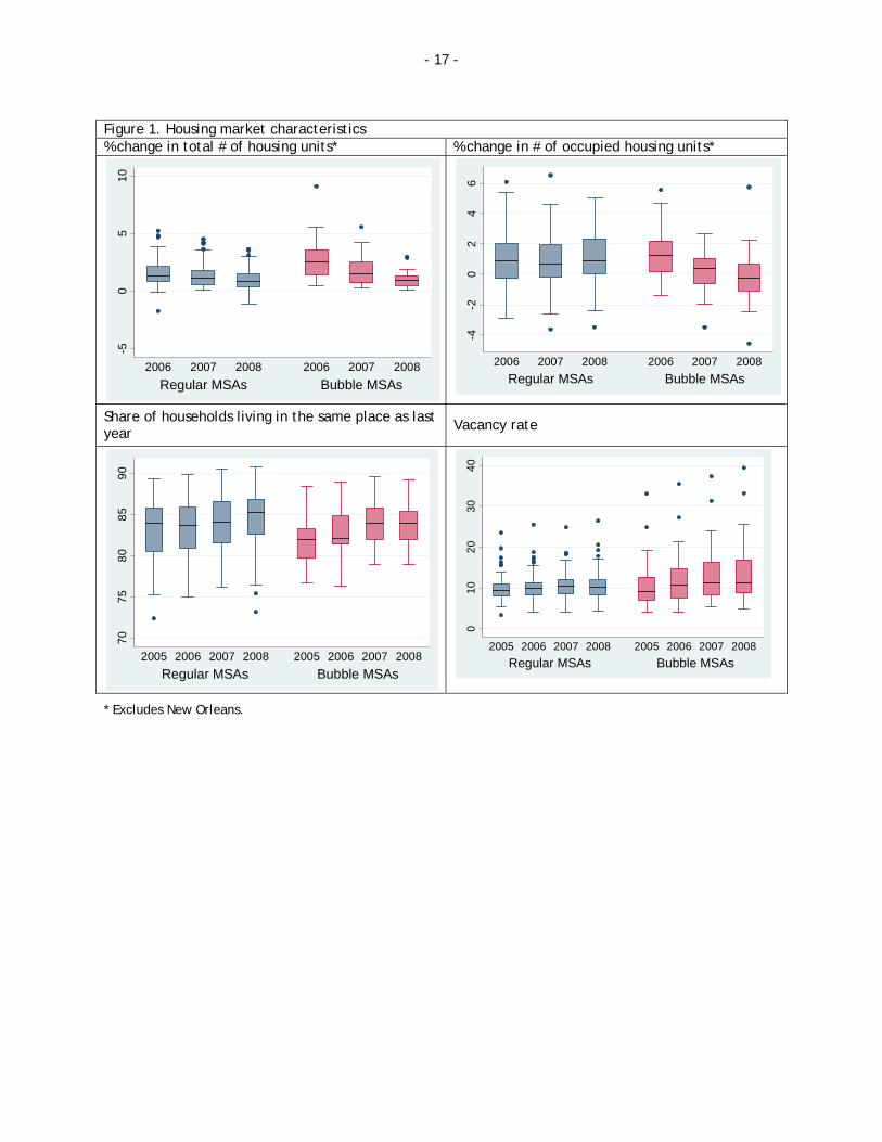
avoid losing information by focusing on scalar measures of changes over time, we also use box plots to

show how distributions of given variables have changed over the 2005-2008 period in bubble versus

other metros -- where the line in the middle of the box shows the median, the bottom and top of the

box show the 25th and 75th percentiles of the distribution respectively, the ends of the whiskers show

the 5th and 95th percentiles, and dots show extreme values beyond these points. An ongoing companion

paper uses the household- and individual-level ACS data to examine effects of the housing-price bust in

a multivariate framework.

Housing wealth and housing costs

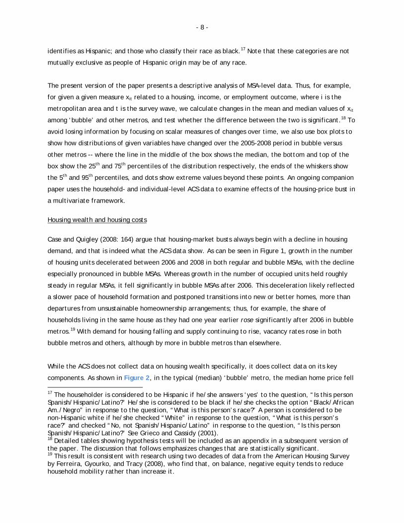
Case and Quigley (2008: 164) argue that housing-market busts always begin with a decline in housing

demand, and that is indeed what the ACS data show. As can be seen in Figure 1, growth in the number

of housing units decelerated between 2006 and 2008 in both regular and bubble MSAs, with the decline

especially pronounced in bubble MSAs. Whereas growth in the number of occupied units held roughly

steady in regular MSAs, it fell significantly in bubble MSAs after 2006. This deceleration likely reflected

a slower pace of household formation and postponed transitions into new or better homes, more than

departures from unsustainable homeownership arrangements; thus, for example, the share of

households living in the same house as they had one year earlier rose significantly after 2006 in bubble

metros.19 With demand for housing falling and supply continuing to rise, vacancy rates rose in both

bubble metros and others, although by more in bubble metros than elsewhere.

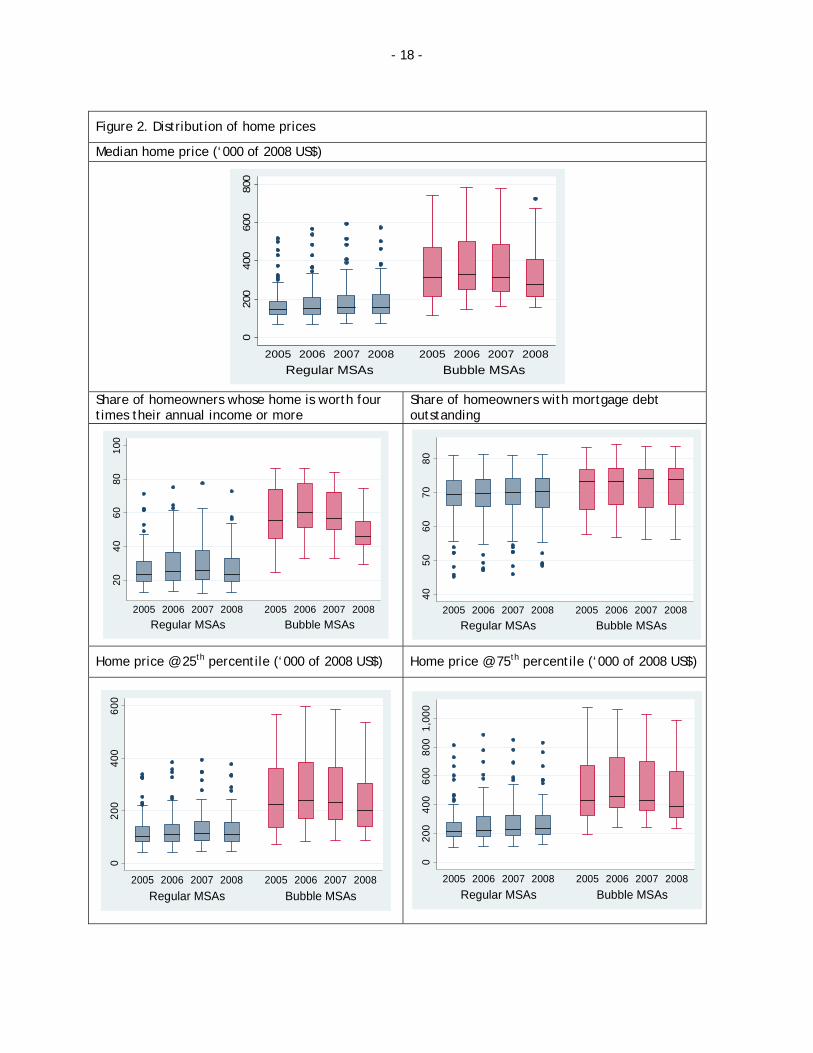
While the ACS does not collect data on housing wealth specifically, it does collect data on its key

components. As shown in Figure 2, in the typical (median) ‘bubble’ metro, the median home price fell 17 The householder is considered to be Hispanic if he/she answers ‘yes’ to the question, “Is this person Spanish/Hispanic/Latino?” He/she is considered to be black if he/she checks the option “Black/African Am./Negro” in response to the question, “What is this person’s race?” A person is considered to be non-Hispanic white if he/she checked “White” in response to the question, “What is this person’s race?” and checked “No, not Spanish/Hispanic/Latino” in response to the question, “Is this person Spanish/Hispanic/Latino?” See Grieco and Cassidy (2001). 18 Detailed tables showing hypothesis tests will be included as an appendix in a subsequent version of the paper. The discussion that follows emphasizes changes that are statistically significant. 19 This result is consistent with research using two decades of data from the American Housing Survey by Ferreira, Gyourko, and Tracy (2008), who find that, on balance, negative equity tends to reduce household mobility rather than increase it.

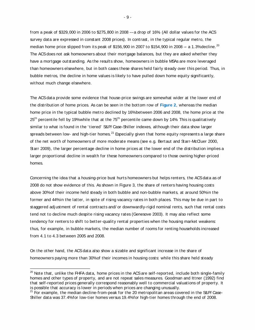
- 9 -

from a peak of $329,000 in 2006 to $275,800 in 2008 -– a drop of 16%. (All dollar values for the ACS

survey data are expressed in constant 2008 prices). In contrast, in the typical regular metro, the

median home price slipped from its peak of $156,900 in 2007 to $154,900 in 2008 –- a 1.3% decline.20

The ACS does not ask homeowners about their mortgage balances, but they are asked whether they

have a mortgage outstanding. As the results show, homeowners in bubble MSAs are more leveraged

than homeowners elsewhere, but in both cases these shares held fairly steady over this period. Thus, in

bubble metros, the decline in home values is likely to have pulled down home equity significantly,

without much change elsewhere.

The ACS data provide some evidence that house-price swings are somewhat wider at the lower end of

the distribution of home prices. As can be seen in the bottom row of Figure 2, whereas the median

home price in the typical bubble metro declined by 16% between 2006 and 2008, the home price at the

25th percentile fell by 19% while that at the 75th percentile came down by 14%. This is qualitatively

similar to what is found in the ‘tiered’ S&P/Case-Shiller indexes, although their data show larger

spreads between low- and high-tier homes.21 Especially given that home equity represents a large share

of the net worth of homeowners of more moderate means (see e.g. Bertaut and Starr-McCluer 2000,

Starr 2009), the larger percentage decline in home prices at the lower end of the distribution implies a

larger proportional decline in wealth for these homeowners compared to those owning higher-priced

homes.

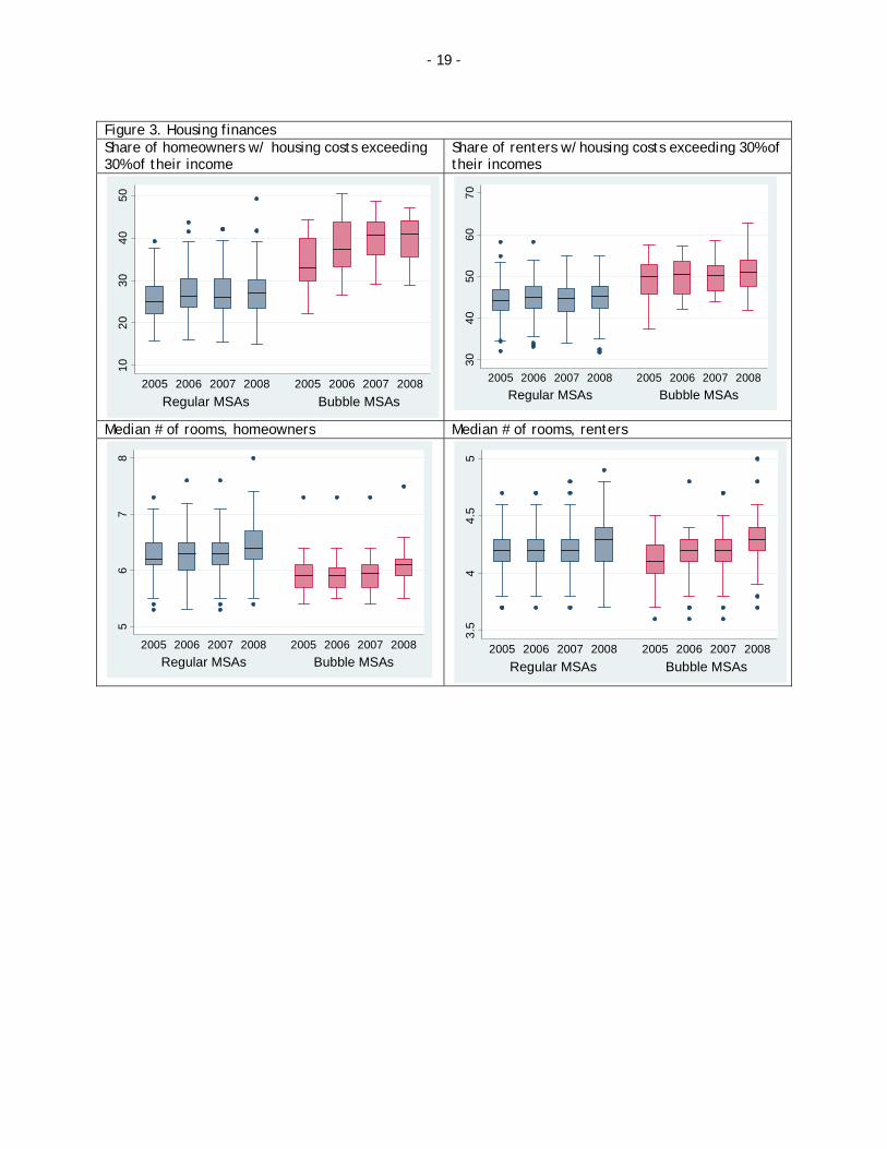
Concerning the idea that a housing-price bust hurts homeowners but helps renters, the ACS data as of

2008 do not show evidence of this. As shown in Figure 3, the share of renters having housing costs

above 30% of their income held steady in both bubble and non-bubble markets, at around 50% in the

former and 44% in the latter, in spite of rising vacancy rates in both places. This may be due in part to

staggered adjustment of rental contracts and/or downwardly-rigid nominal rents, such that rental costs

tend not to decline much despite rising vacancy rates (Genesove 2003). It may also reflect some

tendency for renters to shift to better-quality rental properties when the housing market weakens:

thus, for example, in bubble markets, the median number of rooms for renting households increased

from 4.1 to 4.3 between 2005 and 2008.

On the other hand, the ACS data also show a sizable and significant increase in the share of

homeowners paying more than 30% of their incomes in housing costs: while this share held steady

20 Note that, unlike the FHFA data, home prices in the ACS are self-reported, include both single-family homes and other types of property, and are not repeat sales measures. Goodman and Ittner (1992) find that self-reported prices generally correspond reasonably well to commercial valuations of property. It is possible that accuracy is lower in periods when prices are changing unusually. 21 For example, the median decline-from-peak for the 20 metropolitan areas covered in the S&P/Case-Shiller data was 37.4% for low-tier homes versus 19.4% for high-tier homes through the end of 2008.

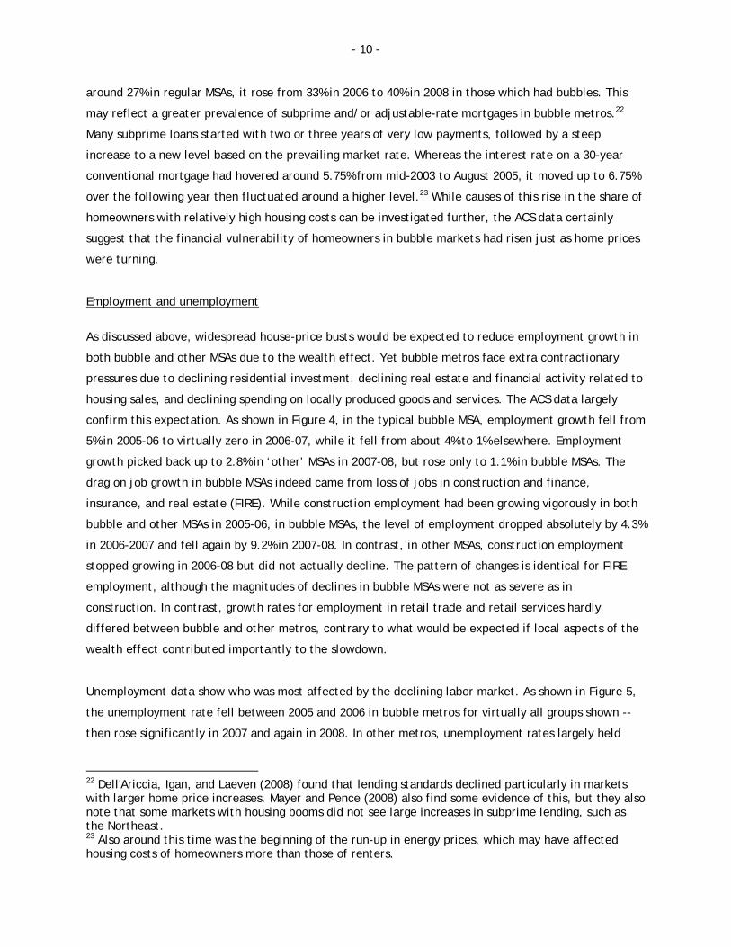
- 10 -

around 27% in regular MSAs, it rose from 33% in 2006 to 40% in 2008 in those which had bubbles. This

may reflect a greater prevalence of subprime and/or adjustable-rate mortgages in bubble metros.22

Many subprime loans started with two or three years of very low payments, followed by a steep

increase to a new level based on the prevailing market rate. Whereas the interest rate on a 30-year

conventional mortgage had hovered around 5.75% from mid-2003 to August 2005, it moved up to 6.75%

over the following year then fluctuated around a higher level.23 While causes of this rise in the share of

homeowners with relatively high housing costs can be investigated further, the ACS data certainly

suggest that the financial vulnerability of homeowners in bubble markets had risen just as home prices

were turning.

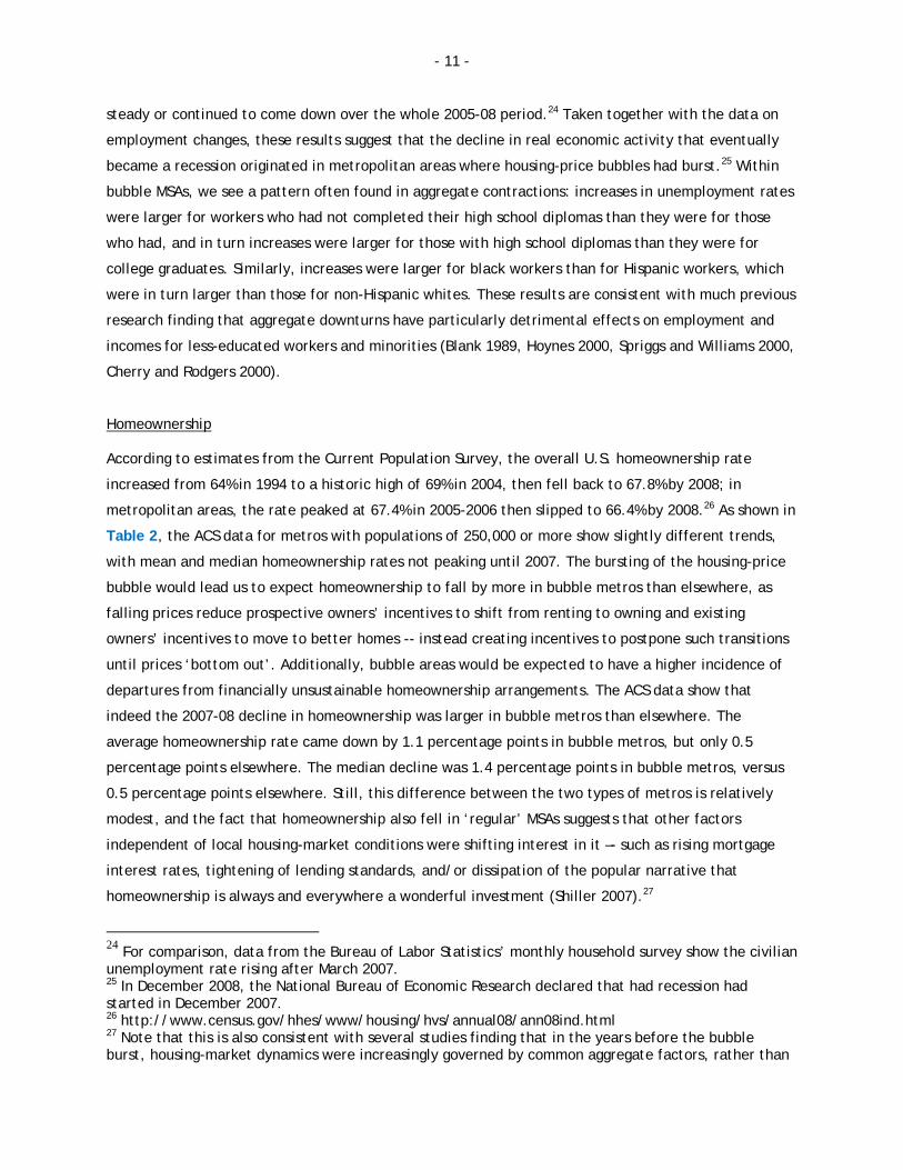
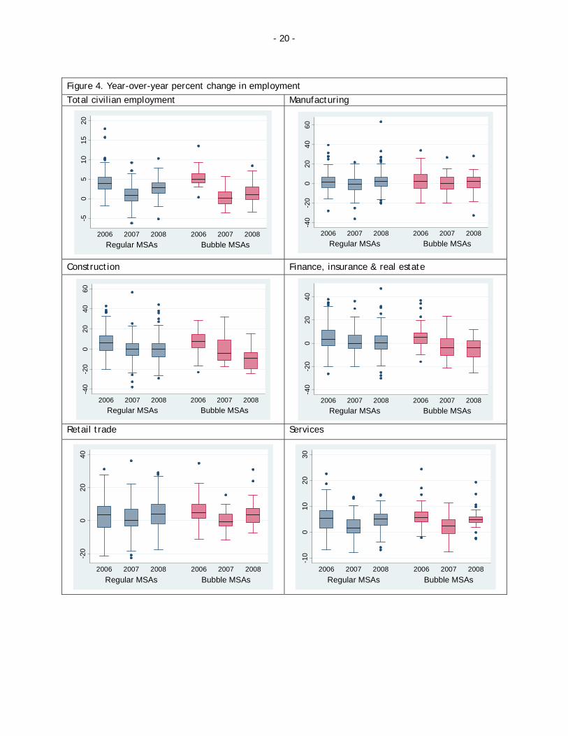
Employment and unemployment

As discussed above, widespread house-price busts would be expected to reduce employment growth in

both bubble and other MSAs due to the wealth effect. Yet bubble metros face extra contractionary

pressures due to declining residential investment, declining real estate and financial activity related to

housing sales, and declining spending on locally produced goods and services. The ACS data largely

confirm this expectation. As shown in Figure 4, in the typical bubble MSA, employment growth fell from

5% in 2005-06 to virtually zero in 2006-07, while it fell from about 4% to 1% elsewhere. Employment

growth picked back up to 2.8% in ‘other’ MSAs in 2007-08, but rose only to 1.1% in bubble MSAs. The

drag on job growth in bubble MSAs indeed came from loss of jobs in construction and finance,

insurance, and real estate (FIRE). While construction employment had been growing vigorously in both

bubble and other MSAs in 2005-06, in bubble MSAs, the level of employment dropped absolutely by 4.3%

in 2006-2007 and fell again by 9.2% in 2007-08. In contrast, in other MSAs, construction employment

stopped growing in 2006-08 but did not actually decline. The pattern of changes is identical for FIRE

employment, although the magnitudes of declines in bubble MSAs were not as severe as in

construction. In contrast, growth rates for employment in retail trade and retail services hardly

differed between bubble and other metros, contrary to what would be expected if local aspects of the

wealth effect contributed importantly to the slowdown.

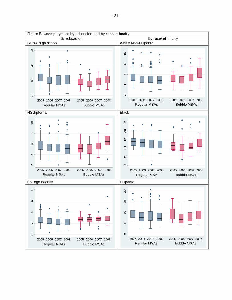
Unemployment data show who was most affected by the declining labor market. As shown in Figure 5,

the unemployment rate fell between 2005 and 2006 in bubble metros for virtually all groups shown --

then rose significantly in 2007 and again in 2008. In other metros, unemployment rates largely held

22 Dell'Ariccia, Igan, and Laeven (2008) found that lending standards declined particularly in markets with larger home price increases. Mayer and Pence (2008) also find some evidence of this, but they also note that some markets with housing booms did not see large increases in subprime lending, such as the Northeast. 23 Also around this time was the beginning of the run-up in energy prices, which may have affected housing costs of homeowners more than those of renters.

- 11 -

steady or continued to come down over the whole 2005-08 period.24 Taken together with the data on

employment changes, these results suggest that the decline in real economic activity that eventually

became a recession originated in metropolitan areas where housing-price bubbles had burst.25 Within

bubble MSAs, we see a pattern often found in aggregate contractions: increases in unemployment rates

were larger for workers who had not completed their high school diplomas than they were for those

who had, and in turn increases were larger for those with high school diplomas than they were for

college graduates. Similarly, increases were larger for black workers than for Hispanic workers, which

were in turn larger than those for non-Hispanic whites. These results are consistent with much previous

research finding that aggregate downturns have particularly detrimental effects on employment and

incomes for less-educated workers and minorities (Blank 1989, Hoynes 2000, Spriggs and Williams 2000,

Cherry and Rodgers 2000).

Homeownership

According to estimates from the Current Population Survey, the overall U.S. homeownership rate

increased from 64% in 1994 to a historic high of 69% in 2004, then fell back to 67.8% by 2008; in

metropolitan areas, the rate peaked at 67.4% in 2005-2006 then slipped to 66.4% by 2008.26 As shown in

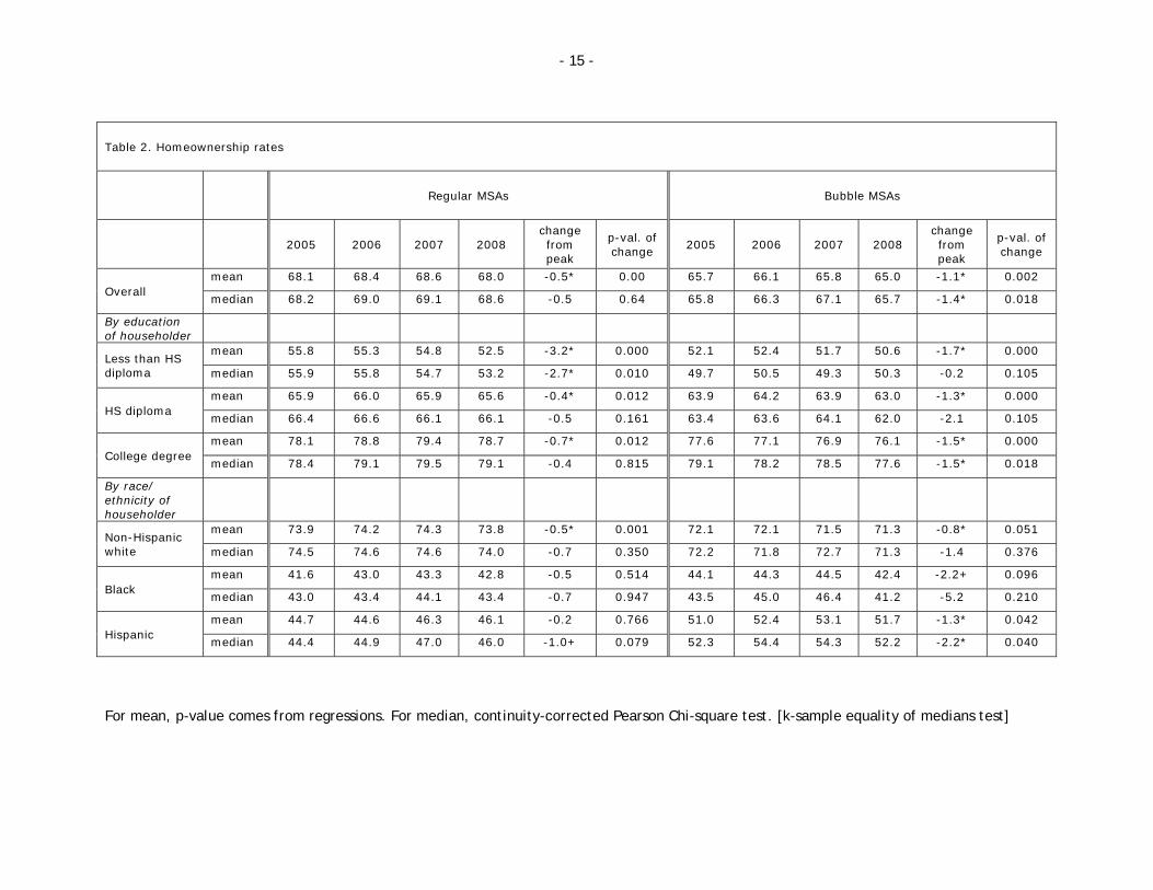
Table 2, the ACS data for metros with populations of 250,000 or more show slightly different trends,

with mean and median homeownership rates not peaking until 2007. The bursting of the housing-price

bubble would lead us to expect homeownership to fall by more in bubble metros than elsewhere, as

falling prices reduce prospective owners’ incentives to shift from renting to owning and existing

owners’ incentives to move to better homes -- instead creating incentives to postpone such transitions

until prices ‘bottom out’. Additionally, bubble areas would be expected to have a higher incidence of

departures from financially unsustainable homeownership arrangements. The ACS data show that

indeed the 2007-08 decline in homeownership was larger in bubble metros than elsewhere. The

average homeownership rate came down by 1.1 percentage points in bubble metros, but only 0.5

percentage points elsewhere. The median decline was 1.4 percentage points in bubble metros, versus

0.5 percentage points elsewhere. Still, this difference between the two types of metros is relatively

modest, and the fact that homeownership also fell in ‘regular’ MSAs suggests that other factors

independent of local housing-market conditions were shifting interest in it –- such as rising mortgage

interest rates, tightening of lending standards, and/or dissipation of the popular narrative that

homeownership is always and everywhere a wonderful investment (Shiller 2007).27

24 For comparison, data from the Bureau of Labor Statistics’ monthly household survey show the civilian unemployment rate rising after March 2007. 25 In December 2008, the National Bureau of Economic Research declared that had recession had started in December 2007. 26 http://www.census.gov/hhes/www/housing/hvs/annual08/ann08ind.html 27 Note that this is also consistent with several studies finding that in the years before the bubble burst, housing-market dynamics were increasingly governed by common aggregate factors, rather than

- 12 -

Perhaps surprisingly, declines in homeownership rates did not differ markedly across households with

differing characteristics: for most types of households in bubble metros, the rate declined by about 1-

1.5 percentage points, while it fell by around 0.5 percentage point for most types of households in

other MSAs. However, more pronounced declines occurred for two specific groups. In bubble MSAs,

homeownership rates fell more steeply for black and Hispanic households than others –- a finding which

is consistent with other studies finding subprime lending to have been concentrated in areas that

experienced bubbles and that had relatively large black and Hispanic populations (e.g. Mayer and

Pence 2008).28 In regular MSAs, there were significant and relatively large declines in mean and median

homeownership among households where the householder had less than a high school education. While

the explanation of this is at present unclear, it is consistent with other evidence in the ACS data of

deteriorating circumstances for this group (see below).

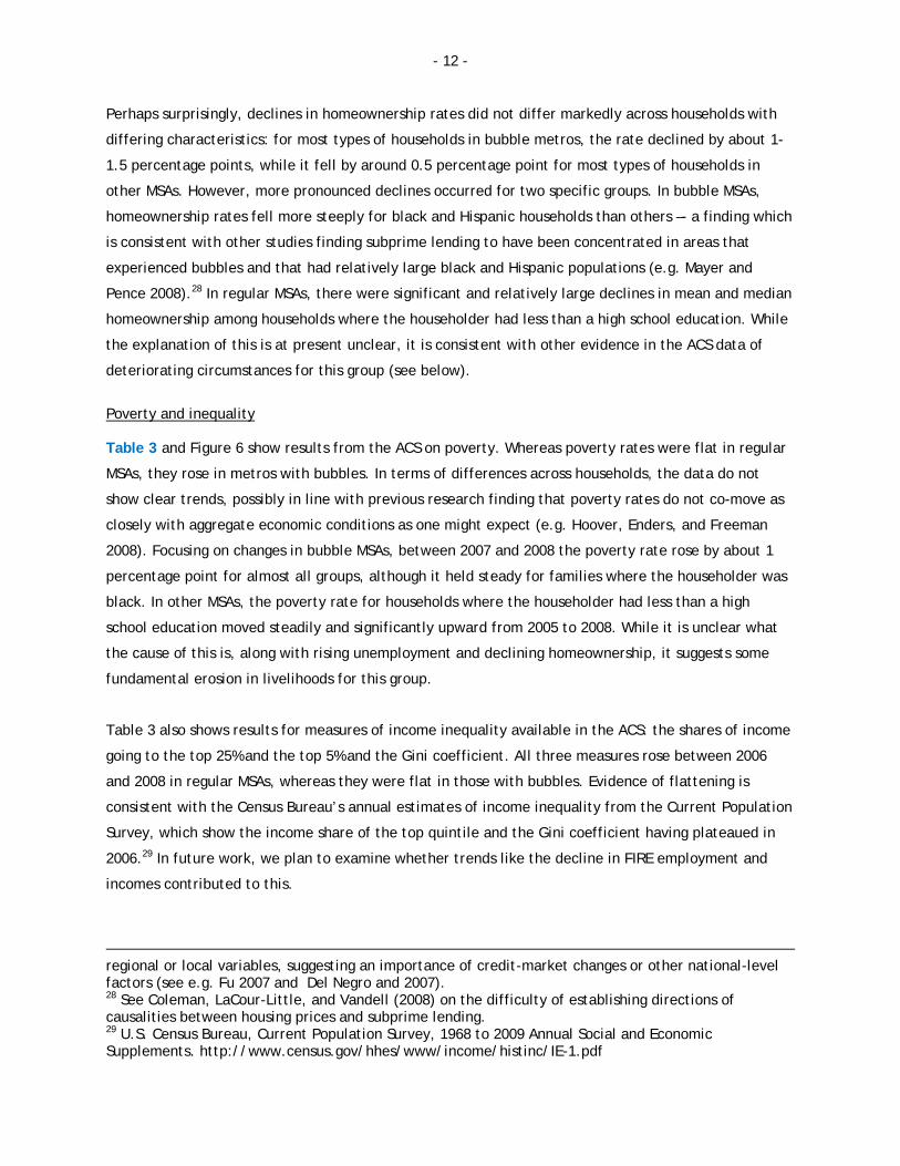
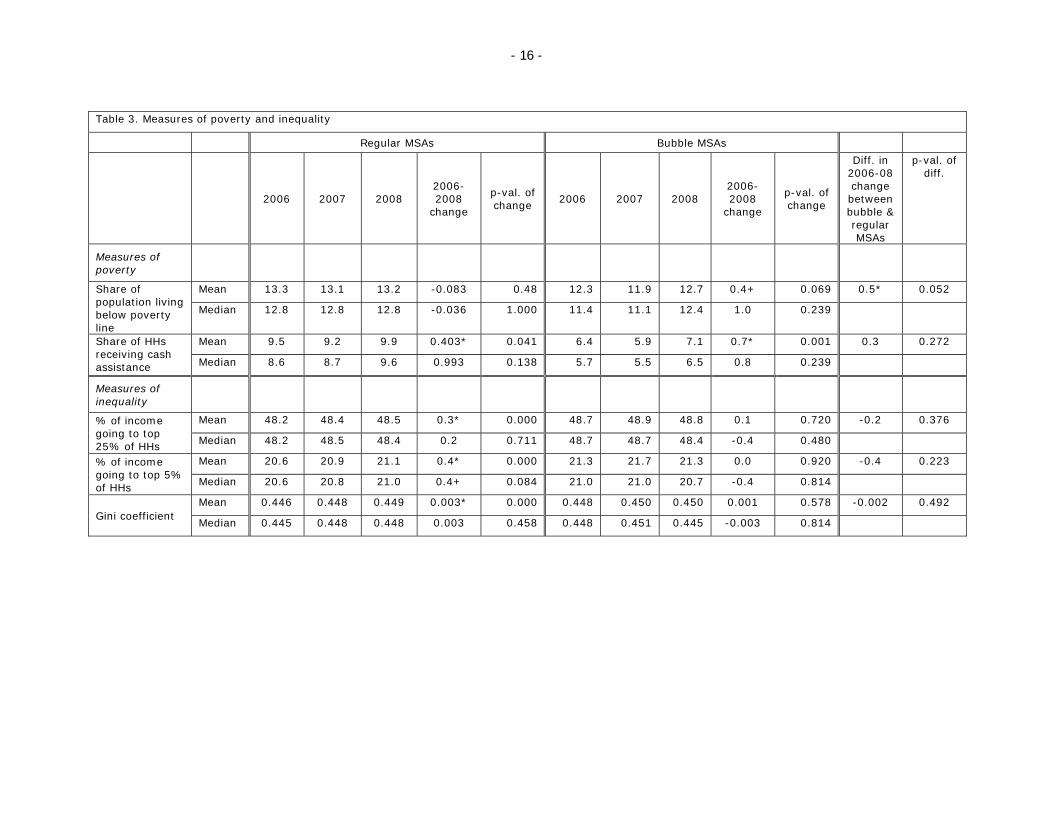
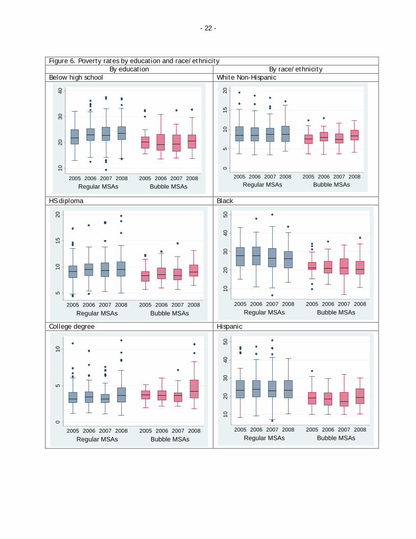
Poverty and inequality Table 3 and Figure 6 show results from the ACS on poverty. Whereas poverty rates were flat in regular

MSAs, they rose in metros with bubbles. In terms of differences across households, the data do not

show clear trends, possibly in line with previous research finding that poverty rates do not co-move as

closely with aggregate economic conditions as one might expect (e.g. Hoover, Enders, and Freeman

2008). Focusing on changes in bubble MSAs, between 2007 and 2008 the poverty rate rose by about 1

percentage point for almost all groups, although it held steady for families where the householder was

black. In other MSAs, the poverty rate for households where the householder had less than a high

school education moved steadily and significantly upward from 2005 to 2008. While it is unclear what

the cause of this is, along with rising unemployment and declining homeownership, it suggests some

fundamental erosion in livelihoods for this group.

Table 3 also shows results for measures of income inequality available in the ACS: the shares of income

going to the top 25% and the top 5% and the Gini coefficient. All three measures rose between 2006

and 2008 in regular MSAs, whereas they were flat in those with bubbles. Evidence of flattening is

consistent with the Census Bureau’s annual estimates of income inequality from the Current Population

Survey, which show the income share of the top quintile and the Gini coefficient having plateaued in

2006.29 In future work, we plan to examine whether trends like the decline in FIRE employment and

incomes contributed to this.

regional or local variables, suggesting an importance of credit-market changes or other national-level factors (see e.g. Fu 2007 and Del Negro and 2007). 28 See Coleman, LaCour-Little, and Vandell (2008) on the difficulty of establishing directions of causalities between housing prices and subprime lending. 29 U.S. Census Bureau, Current Population Survey, 1968 to 2009 Annual Social and Economic Supplements. http://www.census.gov/hhes/www/income/histinc/IE-1.pdf

- 13 -

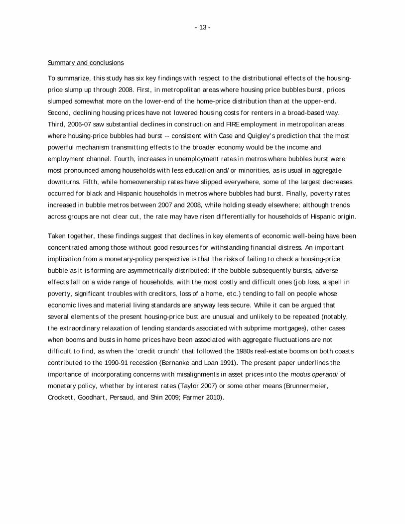
Summary and conclusions

To summarize, this study has six key findings with respect to the distributional effects of the housing-

price slump up through 2008. First, in metropolitan areas where housing price bubbles burst, prices

slumped somewhat more on the lower-end of the home-price distribution than at the upper-end.

Second, declining housing prices have not lowered housing costs for renters in a broad-based way.

Third, 2006-07 saw substantial declines in construction and FIRE employment in metropolitan areas

where housing-price bubbles had burst -- consistent with Case and Quigley’s prediction that the most

powerful mechanism transmitting effects to the broader economy would be the income and

employment channel. Fourth, increases in unemployment rates in metros where bubbles burst were

most pronounced among households with less education and/or minorities, as is usual in aggregate

downturns. Fifth, while homeownership rates have slipped everywhere, some of the largest decreases

occurred for black and Hispanic households in metros where bubbles had burst. Finally, poverty rates

increased in bubble metros between 2007 and 2008, while holding steady elsewhere; although trends

across groups are not clear cut, the rate may have risen differentially for households of Hispanic origin.

Taken together, these findings suggest that declines in key elements of economic well-being have been

concentrated among those without good resources for withstanding financial distress. An important

implication from a monetary-policy perspective is that the risks of failing to check a housing-price

bubble as it is forming are asymmetrically distributed: if the bubble subsequently bursts, adverse

effects fall on a wide range of households, with the most costly and difficult ones (job loss, a spell in

poverty, significant troubles with creditors, loss of a home, etc.) tending to fall on people whose

economic lives and material living standards are anyway less secure. While it can be argued that

several elements of the present housing-price bust are unusual and unlikely to be repeated (notably,

the extraordinary relaxation of lending standards associated with subprime mortgages), other cases

when booms and busts in home prices have been associated with aggregate fluctuations are not

difficult to find, as when the ‘credit crunch’ that followed the 1980s real-estate booms on both coasts

contributed to the 1990-91 recession (Bernanke and Loan 1991). The present paper underlines the

importance of incorporating concerns with misalignments in asset prices into the modus operandi of

monetary policy, whether by interest rates (Taylor 2007) or some other means (Brunnermeier,

Crockett, Goodhart, Persaud, and Shin 2009; Farmer 2010).

- 14 -

Table 1. Categorization of MSAs

Broader bubble definition Narrow bubble definition

Categorization of MSA

Number of MSAs

Median peak (1995=100)

Median % change from

peak to 2008:Q4

Number of MSAs

Median peak (1995=100)

Median % change from

peak to 2008:Q4

Bubble 36 292.2 -27.7 23 309.5 -33.7 Non-bubble 131 182.7 -2.0 144 186.0 -2.4

Source: FHFA all-transaction home price indexes.

- 15 -

Table 2. Homeownership rates

Regular MSAs Bubble MSAs

2005 2006 2007 2008

change from peak

p-val. of change

2005 2006 2007 2008 change from peak

p-val. of change

Overall mean 68.1 68.4 68.6 68.0 -0.5* 0.00 65.7 66.1 65.8 65.0 -1.1* 0.002

median 68.2 69.0 69.1 68.6 -0.5 0.64 65.8 66.3 67.1 65.7 -1.4* 0.018

By education of householder

Less than HS diploma

mean 55.8 55.3 54.8 52.5 -3.2* 0.000 52.1 52.4 51.7 50.6 -1.7* 0.000

median 55.9 55.8 54.7 53.2 -2.7* 0.010 49.7 50.5 49.3 50.3 -0.2 0.105

HS diploma mean 65.9 66.0 65.9 65.6 -0.4* 0.012 63.9 64.2 63.9 63.0 -1.3* 0.000

median 66.4 66.6 66.1 66.1 -0.5 0.161 63.4 63.6 64.1 62.0 -2.1 0.105

College degree mean 78.1 78.8 79.4 78.7 -0.7* 0.012 77.6 77.1 76.9 76.1 -1.5* 0.000

median 78.4 79.1 79.5 79.1 -0.4 0.815 79.1 78.2 78.5 77.6 -1.5* 0.018

By race/ ethnicity of householder

Non-Hispanic white

mean 73.9 74.2 74.3 73.8 -0.5* 0.001 72.1 72.1 71.5 71.3 -0.8* 0.051

median 74.5 74.6 74.6 74.0 -0.7 0.350 72.2 71.8 72.7 71.3 -1.4 0.376

Black mean 41.6 43.0 43.3 42.8 -0.5 0.514 44.1 44.3 44.5 42.4 -2.2+ 0.096

median 43.0 43.4 44.1 43.4 -0.7 0.947 43.5 45.0 46.4 41.2 -5.2 0.210

Hispanic mean 44.7 44.6 46.3 46.1 -0.2 0.766 51.0 52.4 53.1 51.7 -1.3* 0.042

median 44.4 44.9 47.0 46.0 -1.0+ 0.079 52.3 54.4 54.3 52.2 -2.2* 0.040

For mean, p-value comes from regressions. For median, continuity-corrected Pearson Chi-square test. [k-sample equality of medians test]

- 16 -

Table 3. Measures of poverty and inequality

Regular MSAs Bubble MSAs

2006 2007 2008 2006-2008

change

p-val. of change

2006 2007 2008 2006-2008

change

p-val. of change

Diff. in 2006-08 change between bubble & regular MSAs

p-val. of diff.

Measures of poverty

Share of population living below poverty line

Mean 13.3 13.1 13.2 -0.083 0.48 12.3 11.9 12.7 0.4+ 0.069 0.5* 0.052

Median 12.8 12.8 12.8 -0.036 1.000 11.4 11.1 12.4 1.0 0.239

Share of HHs receiving cash assistance

Mean 9.5 9.2 9.9 0.403* 0.041 6.4 5.9 7.1 0.7* 0.001 0.3 0.272

Median 8.6 8.7 9.6 0.993 0.138 5.7 5.5 6.5 0.8 0.239

Measures of inequality

% of income going to top 25% of HHs

Mean 48.2 48.4 48.5 0.3* 0.000 48.7 48.9 48.8 0.1 0.720 -0.2 0.376

Median 48.2 48.5 48.4 0.2 0.711 48.7 48.7 48.4 -0.4 0.480

% of income going to top 5% of HHs

Mean 20.6 20.9 21.1 0.4* 0.000 21.3 21.7 21.3 0.0 0.920 -0.4 0.223

Median 20.6 20.8 21.0 0.4+ 0.084 21.0 21.0 20.7 -0.4 0.814

Gini coefficient Mean 0.446 0.448 0.449 0.003* 0.000 0.448 0.450 0.450 0.001 0.578 -0.002 0.492

Median 0.445 0.448 0.448 0.003 0.458 0.448 0.451 0.445 -0.003 0.814

- 17 -

Figure 1. Housing market characteristics % change in total # of housing units* % change in # of occupied housing units*

-50

51

0

Regular MSAs Bubble MSAs2006 2007 2008 2006 2007 2008

-4-2

02

46


Share of households living in the same place as last year

Vacancy rate

70

75

80

85

90

Regular MSAs Bubble MSAs2005 2006 2007 2008 2005 2006 2007 2008

01

02

03

04

0


* Excludes New Orleans.

- 18 -

Figure 2. Distribution of home prices

Median home price (‘000 of 2008 US$)

0200

400

600

800


Share of homeowners whose home is worth four times their annual income or more

Share of homeowners with mortgage debt outstanding

20

40

60

80

100


40

50

60

70

80


Home price @ 25th percentile (‘000 of 2008 US$) Home price @ 75th percentile (‘000 of 2008 US$)

02

004

006

00


02

004

006

008

001

,00

0


- 19 -

Figure 3. Housing finances Share of homeowners w/ housing costs exceeding 30% of their income

Share of renters w/housing costs exceeding 30% of their incomes

10

20

30

40

50


30

40

50

60

70


Median # of rooms, homeowners Median # of rooms, renters

56

78


3.5

44

.55


- 20 -

Figure 4. Year-over-year percent change in employment

Total civilian employment Manufacturing

-50

51

01

52

0


-40

-20

02

04

06

0


Construction Finance, insurance & real estate

-40

-20

02

04

06

0


-40

-20

02

04

0


Retail trade Services

-20

02

04

0


-10

01

02

03

0


- 21 -

Figure 5. Unemployment by education and by race/ethncity

By education By race/ethnicity Below high school White Non-Hispanic

01

02

03

0


24

68

10


HS diploma Black

24

68

10


05

10

15

20

25

Regular MSA Bubble MSAs2005 2006 2007 2008 2005 2006 2007 2008

College degree Hispanic

02

46

8


05

10

15

20


- 22 -

Figure 6. Poverty rates by education and race/ethnicity

By education By race/ethnicity Below high school White Non-Hispanic

10

20

30

40


05

10

15

20


HS diploma Black

51

01

52

0


10

20

30

40

50


College degree Hispanic

05

10


10

20

30

40

50


- 23 -

REFERENCES Baker, Dean, and David Rosnick (2008). “The Impact of the Housing Crash on Family Wealth.” Center for Economic and Policy Research (Washington, DC), CEPR Reports and Issue Briefs. Barlevy, Gadi (2004). “The cost of business cycles and the benefits of stabilization: a survey.” NBER Working Paper No. 10926. Bernanke, Ben (2002). “Asset-price ‘bubbles’ and monetary policy.” Address to the New York Chapter of the National Association for Business Economics, New York, New York (Oct. 15). Bernanke, Ben and Cara Lown (1991). “The Credit Crunch,” Brookings Papers on Economic Activity, no. 2, pp. 204-39. Bertaut, Carol and Martha Starr-McCluer (2000). "Household Portfolios in the United States.” In Luigi Guiso, Michael Haliassos, and Tullio Jappelli,eds., Household Portfolios. Cambridge: MIT Press.

Blank, Rebecca M. (1989). ”Disaggregating the Effect of the Business Cycle on the Distribution of Income,” Economica, vol. 56, no. 2, pp141-163, May 1989.

Bostic, Raphael, Stuart Gabriel, and Gary Painter (2009). “Housing Wealth, Financial Wealth, and Consumption: New Evidence from Micro Data,” Regional Science and Urban Economics, vol. 39, no. 1 (Jan.), pp. 79-89. Brunnermeier, Marcus, Andrew Crockett, Charles Goodhart, Avinash Persaud and Hyun Shin (2009), “The Fundamental Principles of Financial Regulation.” International Center for Monetary and Banking Studies, Geneva Report on the World Economy, No.11 (Jan.). Carroll, Christopher D., Misuzu Otsuka, Jirka Slacalek (2006). “How Large Is the Housing Wealth Effect? A New Approach.” NBER Working Paper No. 12746. Case, Karl E. and Leah Cook (1989). “The Distributional Effects of Housing Price Booms: Winners and Losers in Boston, 1980-88,” New England Economic Review, May, pp. 3–12. Case, Karl E. and Christopher Mayer (1996). “Housing price dynamics within a metropolitan area,” Regional Science and Urban Economics, Vol. 26, No. 3-4 (June), pp. 387-407. Case, Karl E. and John Quigley (2008). “How Housing Booms Unwind: Income Effects, Wealth Effects, and Feedbacks through Financial Markets.” European Journal of Housing Policy, June. Case, Karl E., John M. Quigley, and Robert J. Shiller (2005), “Comparing Wealth Effects: The Stock Market versus the Housing Market,” Advances in Macroeconomics, 5(1), 1–32. Cherry, Robert D. and William M. Rodgers, eds. (2000). Prosperity for all? The economic boom and African Americans. New York, NY: Russell Sage Foundation. Coleman, Major, Michael LaCour-Little, Kerry D. Vandell (2008). “Subprime Lending and the Housing Bubble: Tail Wags Dog?” Journal of Housing Economics, vol. 17, no. 4 (Dec.), pp. 272-90. Cutler, David M. and Lawrence F. Katz., “Macroeconomic Performance and the Disadvantaged”, Brookings Papers on Economic Activity, 1991, 1-74.

Del Negro, Marco and Christopher Otrok (2007). “99 Luftballons: Monetary policy and the house price boom across U.S. states,” Journal of Monetary Economics, Vol. 54, No. 7 (Oct.), pp. 1962-1985.

- 24 -

Dell'Ariccia, Giovanni, Deniz Igan, and Luc Laeven (2008). “Credit Booms and Lending Standards: Evidence From The Subprime Mortgage Market," C.E.P.R. Discussion Paper No. 6683.

Evans, Charles L. (2009). “Should Monetary Policy Prevent Bubbles?” Address at a conference on “Asset price bubbles and monetary policy,” organized by the Banque de France and the Federal Reserve Bank of Chicago, Paris, France (Nov. 13).

Fair, Ray (2004). Estimating How the Macroeconomy Works (Cambridge, MA: Harvard University Press).

Farmer, Roger (2010). Expectations, Employment and Prices. Oxford, UK: Oxford University Press, forthcoming.

Ferreira, Fernando, Joseph Gyourko, and Joseph Tracy (2008). "Housing Busts and Household Mobility," NBER Working Paper No. 14310. Fu, Dong (2007). “National, regional and metro-specific factors of the U.S. housing market,” Federal Reserve Bank of Dallas, Working Papers: 0707.

Genesove, David (2003). “The Nominal Rigidity of Apartment Rents,” Review of Economics and Statistics, Vol. 85, No. 4 (Nov.), pp. 844-853

Glaeser, Edward L., Joseph Gyourko, and Albert Saiz (2008). "Housing supply and housing bubbles," Journal of Urban Economics, vol. 64, No. 2 (Sept.), pp. 198-217.

Allen C. Goodman, and Thomas G. Thibodeau (2008). “Where are the Speculative Bubbles in U.S. Housing Markets?” Journal of Housing Economics, Vol. 17, No. 2 (June), pp. 117-137.

Gramlich, Edward (2007). Subprime Mortgages: America's Latest Boom and Bust. Washington, DC: Urban Institute Press. Grieco, Elizabeth M. and Rachel C. Cassidy (2001). “Overview of Race and Hispanic Origin.” Census 2000 Brief C2KBR/01-1 (March). http://www.census.gov/prod/2001pubs/c2kbr01-1.pdf Gyourko, Joseph and Joseph Tracy (1999). "A look at real housing prices and incomes: some implications for housing affordability and quality," Federal Reserve Bank of New York Economic Policy Review, Vol. 5, No. 3 (Sept.), pp. 63-77. http://www.newyorkfed.org/research/epr/99v05n3/9909gyou.pdf Himmelberg, Charles, Christopher Mayer, and Todd Sinai (2005). “Assessing High House Prices: Bubbles, Fundamentals and Misperceptions,” Journal of Economic Perspectives, vol. 19, no. 4 (Fall), pp. 67-92. Hoover, Gary A., Walter Enders, and Donald G. Freeman. 2008. "Non-white Poverty and the Macroeconomy: The Impact of Growth," American Economic Review, Vol. 98, No. 2 (May), pp. 398–402. Hoynes, Hilary W. (2000). “The Employment, Earnings, and Income of Less Skilled Workers over the Business Cycle.” In David Card and Rebecca Blank, eds., Finding jobs: Work and welfare reform. New York, NY: Russell Sage Foundation, pp. 23-71 Hsieh, Chang-Tai, and Enrico Moretti (2003). “Can Free Entry Be Inefficient? Fixed Commissions and Social Waste in the Real Estate Industry,” Journal of Political Economy, vol. 111, no. 5 (Oct.), pp. 1076-1122. Imrohoroglu, Ayse (2008). "Welfare costs of business cycles." In Steven N. Durlauf and Lawrence

- 25 -

E. Blume, eds., The New Palgrave Dictionary of Economics Online (2nd edition of the New Palgrave Dictionary). Palgrave Macmillan.

Kohn, Donald L. (2008). “Monetary Policy and Asset Prices Revisited.” Speech at the Cato Institute’s 26th Annual Monetary Policy Conference, Washington, D.C. (Nov. 19).

Krusell, Per, Toshihiko Mukoyama, Aysegul Sahin, Anthony Smith, Jr. (2009). “Revisiting the Welfare Effects of Eliminating Business Cycles,” Review of Economic Dynamics, vol. 12, no. 3 (July), pp. 393-404. Lansing, Kevin (2008). “Monetary Policy and Asset Prices,” Federal Reserve Bank of San Francisco Economic Letter No. 2008-34 (Oct. 31). Mayer, Christopher J. (1993). “Taxes, Income Distribution, and the Real Estate Cycle: Why All Houses Do Not Appreciate at the Same Rate,” New England Economic Review, May-June, pp. 39-50. ________________ and Karen Pence (2008). “Subprime Mortgages: What, Where, and to Whom?” NBER Working Paper No. 14083 (June). Mishkin, Frederic S. (2008). “How Should We Respond to Asset Price Bubbles?” Speech at the Wharton Financial Institutions Center and Oliver Wyman Institute’s Annual Financial Risk Roundtable, Philadelphia, PA (May 15). Muellbauer, John (2008). “Housing, Credit and Consumer Expenditure.” C.E.P.R. Discussion Paper No. 6782. Quigley, John M. and Steven Raphael (2001). “The Economics of Homelessness: The Evidence from North America,” European Journal of Housing Policy, vol. 1, no. 3 (Dec.), pp. 323-36.

Rudebusch, Glenn (2005). “Monetary Policy and Asset Price Bubbles,” Federal Reserve Bank of San Francisco Economic Letter No. 2005-18 (Aug. 5)

Sheiner, Louise (1995). “Housing prices and the savings of renters,” Journal of Urban Economics, Vol. 38, No. 1, pp. 94-125. Shiller, Robert J. (2004). “Household Reaction to Changes in Housing Wealth.” Cowles Foundation, Yale University, Cowles Foundation Discussion Papers: 1459. ______________ (2007). “Understanding Recent Trends in House Prices and Home Ownership.” Cowles Foundation Discussion Paper No. 1630. Spriggs, William E. and Rhonda M. Williams (2000). “What Do We Need to Explain About African American Unemployment,” in Robert Cherry and William M. Rodgers, III (eds.), Prosperity for All? The Economic Boom and African Americans. New York: Russell Sage, pp. 188-207. Starr, Martha A. (2009). “Lifestyle conformity and lifecycle saving: A Veblenian perspective,” Cambridge Journal of Economics, Vol. 33, No. 1 (Jan.), pp. 25-49

Yellen, Janet (2009). “A Minsky Meltdown: Lessons for Central Bankers.” Presentation for the Levy Institute’s 18th annual Hyman P. Minsky Conference on the State of the U.S. and World Economies, “Meeting the Challenges of the Financial Crisis” (April 16). http://www.frbsf.org/news/speeches/2009/0416.html

- 26 -

Appendix Table 1. Estimates of the housing-wealth effect

Billions of current U.S. dollars

PCE deflator

(1995=100)

Wealth effect in chained 2005 US$

Real PCE (billions of

chained 2005 U$)

Real PCE, adding in

what was lost to the wealth

effect (5)+(6)

Actual growth rate

of PCE

Growth that would have

been registered had there been no wealth effect

Slower growth in

consumption due to wealth effect (9)-(8)

Flow of funds

estimate of home equity

Change in home equity

Estimated wealth effect on spending from current and lagged wealth changes

(1) (2) (3) (4) (5) (6) (7) (8) (9) (10)

200601 13463.5

200602 13190.8 ‐272.8 ‐5.5 101.8 ‐5.4 9035.0 9040.4 2.6 2.7 ‐0.1

200603 12983.6 ‐207.2 ‐15.1 102.6 ‐14.7 9090.7 9105.4 2.5 2.7 ‐0.2

200604 13117.2 133.6 ‐19.3 103.3 ‐18.6 9181.6 9200.2 3.3 3.5 ‐0.2

200701 12472.0 ‐645.2 ‐34.3 103.3 ‐33.2 9265.1 9298.3 3.1 3.5 ‐0.4

200702 11946.1 ‐525.9 ‐61.2 104.3 ‐58.7 9291.5 9350.2 2.8 3.4 ‐0.6

200703 11231.2 ‐714.9 ‐94.5 105.1 ‐90.0 9335.6 9425.6 2.7 3.5 ‐0.8

200704 10492.8 ‐738.4 ‐135.8 105.7 ‐128.5 9363.6 9492.1 2.0 3.2 ‐1.2

200801 9384.6 ‐1108.2 ‐192.1 107.0 ‐179.5 9349.6 9529.1 0.9 2.5 ‐1.6

200802 8520.3 ‐864.3 ‐232.8 108.0 ‐215.6 9351.0 9566.6 0.6 2.3 ‐1.7

200803 7656.0 ‐864.2 ‐280.7 109.0 ‐257.5 9267.7 9525.2 ‐0.7 1.1 ‐1.8

200804 6607.4 ‐1048.6 ‐363.2 110.3 ‐329.4 9195.3 9524.7 ‐1.8 0.3 ‐2.1

200901 5256.8 ‐1350.6 ‐394.8 108.9 ‐362.7 9209.2 9571.9 ‐1.5 0.4 ‐2.0

200902 5795.4 538.6 ‐416.7 108.4 ‐384.2 9189.0 9573.2 ‐1.7 0.1 ‐1.8

200903 6213.3 417.9 ‐401.3 108.8 ‐368.8 9256.0 9624.8 ‐0.1 1.0 ‐1.2

Assumed effects by quarter are Q1: .02, Q2: .04, Q3: .05, Q4: .06, Q5: .07, Q6: .075. Q7: .078, Q8: .08

- 27 -

- 28 -

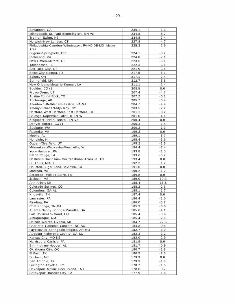
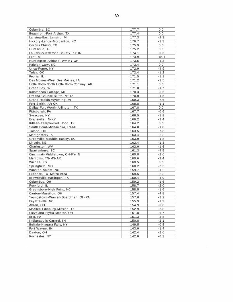
Appendix Table 2. Categorization of MSAs by bubble definitions

Peak index value

(1995=100)

% decline from peak thru

2008:Q4 Metros classified as having bubbles under both narrow and broad definitions

Bakersfield, CA 280.4 -35.8 Cape Coral-Fort Myers, FL 308.3 -43.5 Deltona-Daytona Beach-Ormond Beach, FL 291.7 -25.3 Fresno, CA 286.2 -32.6 Las Vegas-Paradise, NV 258.5 -37.1 Los Angeles-Long Beach-Santa Ana, CA 338.4 -24.0 Miami-Fort Lauderdale-Pompano Beach, FL 332.9 -28.9 Modesto, CA 312.3 -49.4 Naples-Marco Island, FL 370.1 -41.9 Oxnard-Thousand Oaks-Ventura, CA 325.4 -29.2 Palm Bay-Melbourne-Titusville, FL 279.5 -31.1 Port St. Lucie, FL 292.7 -33.7 Riverside-San Bernardino-Ontario, CA 332.7 -40.1 Sacramento--Arden-Arcade--Roseville, CA 291.3 -34.1 Salinas, CA 356.6 -43.5 San Diego-Carlsbad-San Marcos, CA 322.4 -26.0 San Francisco-Oakland-Fremont, CA 313.2 -20.4 Santa Barbara-Santa Maria-Goleta, CA 346.9 -31.4 Santa Rosa-Petaluma, CA 302.1 -27.6 Bradenton-Sarasota-Venice, FL 309.5 -35.9 Stockton, CA 308.7 -51.7 Vallejo-Fairfield, CA 314.8 -42.8 Visalia-Porterville, CA 252.6 -27.8 Metros classified as having bubbles under the broad definition only

Jacksonville, FL 270.5 -12.0 Lakeland-Winter Haven, FL 256.1 -17.2 Ocala, FL 271.3 -17.6 Orlando-Kissimmee, FL 284.5 -21.9 Pensacola-Ferry Pass-Brent, FL 230.8 -14.2 Phoenix-Mesa-Scottsdale, AZ 295.6 -22.4 Providence-New Bedford-Fall River, RI-MA 259.0 -11.0 Reno-Sparks, NV 252.0 -24.9 San Jose-Sunnyvale-Santa Clara, CA 315.7 -14.7 Tampa-St. Petersburg-Clearwater, FL 291.3 -23.3 Tucson, AZ 242.6 -12.2 Washington-Arlington-Alexandria, DC-VA-MD-WV 277.7 -14.6 Worcester, MA 246.1 -10.3

Metros without bubbles

Charleston-North Charleston-Summerville, SC 274.5 -2.7 Atlantic City-Hammonton, NJ 274.3 -7.4 Seattle-Tacoma-Bellevue, WA Metro Area 262.8 -5.0 Virginia Beach-Norfolk-Newport News, VA-NC 259.0 -3.0 Baltimore-Towson, MD 257.6 -5.8 Manchester-Nashua, NH 254.4 -7.5 Poughkeepsie-Newburgh-Middletown, NY 254.2 -9.3 Portland-Vancouver-Beaverton, OR-WA 246.6 -5.2 Asheville, NC 246.6 -0.2 Portland-South Portland-Biddeford, ME 246.4 -2.9 Bridgeport-Stamford-Norwalk, CT 243.3 -6.9 Wilmington, NC 242.9 -4.8 Duluth, MN-WI 242.6 -0.5 Boston-Cambridge-Quincy, MA-NH 238.0 -6.8 New York Metro Area 238.0 -6.8

- 29 -

Savannah, GA 236.1 -1.3 Minneapolis-St. Paul-Bloomington, MN-WI 234.8 -8.7 Trenton-Ewing, NJ 234.8 -7.4 Norwich-New London, CT 227.8 -4.7 Philadelphia-Camden-Wilmington, PA-NJ-DE-MD Metro Area

225.3 -2.9

Eugene-Springfield, OR 224.1 -3.2 Richmond, VA 224.0 -2.1 New Haven-Milford, CT 223.5 -6.1 Tallahassee, FL 222.3 -6.1 Salt Lake City, UT 221.9 -3.4 Boise City-Nampa, ID 217.5 -6.1 Salem, OR 217.1 -2.4 Springfield, MA 212.7 -5.8 New Orleans-Metairie-Kenner, LA 211.1 -1.4 Boulder, CO /1 208.5 0.0 Provo-Orem, UT 207.4 -4.7 Austin-Round Rock, TX 207.2 -0.1 Anchorage, AK 205.7 -0.4 Allentown-Bethlehem-Easton, PA-NJ 204.7 -4.4 Albany-Schenectady-Troy, NY 203.5 -2.2 Hartford-West Hartford-East Hartford, CT 201.1 -3.2 Chicago-Naperville-Joliet, IL-IN-WI 201.0 -4.1 Kingsport-Bristol-Bristol, TN-VA 200.4 0.0 Denver-Aurora, CO /1 200.3 -1.4 Spokane, WA 200.2 -1.3 Roanoke, VA 199.2 0.0 Mobile, AL 199.1 -3.7 Honolulu, HI 198.4 -3.6 Ogden-Clearfield, UT 195.2 -1.5 Milwaukee-Waukesha-West Allis, WI 194.4 -2.4 York-Hanover, PA 193.8 -1.5 Baton Rouge, LA 193.6 -0.7 Nashville-Davidson--Murfreesboro--Franklin, TN 193.4 0.0 St. Louis, MO-IL 192.2 -1.2 Houston-Sugar Land-Baytown, TX 191.0 0.0 Madison, WI 190.2 -1.2 Scranton--Wilkes-Barre, PA 189.8 0.0 Jackson, MS 189.0 -10.3 Ann Arbor, MI 188.4 -16.8 Colorado Springs, CO 188.2 -2.6 Columbus, GA-AL 188.1 -1.7 Knoxville, TN 187.4 0.0 Lancaster, PA 186.4 -1.0 Reading, PA 186.0 -3.7 Chattanooga, TN-GA 185.9 -3.0 Atlanta-Sandy Springs-Marietta, GA 185.6 -4.1 Fort Collins-Loveland, CO 185.4 -0.6 Albuquerque, NM 185.4 -2.6 Detroit-Warren-Livonia, MI 184.7 -22.5 Charlotte-Gastonia-Concord, NC-SC 184.3 -0.4 Fayetteville-Springdale-Rogers, AR-MO 182.7 -3.9 Augusta-Richmond County, GA-SC 182.3 -2.2 Kansas City, MO-KS 182.0 -2.9 Harrisburg-Carlisle, PA 181.9 0.0 Birmingham-Hoover, AL 181.7 -0.9 Oklahoma City, OK 180.7 -1.8 El Paso, TX 180.5 -2.5 Durham, NC 179.9 0.0 San Antonio, TX 179.3 -1.8 Lexington-Fayette, KY 178.7 -1.5 Davenport-Moline-Rock Island, IA-IL 178.0 -0.7 Shreveport-Bossier City, LA 177.9 -1.8

- 30 -

Columbia, SC 177.7 0.0 Beaumont-Port Arthur, TX 177.4 0.0 Lansing-East Lansing, MI 177.3 -9.3 Hickory-Lenoir-Morganton, NC 176.7 -1.3 Corpus Christi, TX 175.9 0.0 Huntsville, AL 175.2 0.0 Louisville/Jefferson County, KY-IN 174.1 -0.6 Flint, MI 173.9 -18.1 Huntington-Ashland, WV-KY-OH 173.5 -1.3 Raleigh-Cary, NC 173.4 0.0 Utica-Rome, NY 172.9 -4.9 Tulsa, OK 172.4 -1.2 Peoria, IL 171.5 -1.1 Des Moines-West Des Moines, IA 171.2 -1.5 Little Rock-North Little Rock-Conway, AR 171.1 0.0 Green Bay, WI 171.0 -1.7 Kalamazoo-Portage, MI 170.3 -5.6 Omaha-Council Bluffs, NE-IA 170.0 -1.5 Grand Rapids-Wyoming, MI 169.3 -7.6 Fort Smith, AR-OK 168.8 -1.1 Dallas-Fort Worth-Arlington, TX 167.8 0.0 Pittsburgh, PA 167.7 -0.6 Syracuse, NY 166.5 -1.8 Evansville, IN-KY 166.2 -3.4 Killeen-Temple-Fort Hood, TX 164.2 0.0 South Bend-Mishawaka, IN-MI 164.0 -1.8 Toledo, OH 163.5 -7.3 Montgomery, AL 163.4 0.0 Greenville-Mauldin-Easley, SC 163.0 -1.8 Lincoln, NE 162.4 -1.3 Charleston, WV 162.0 -1.6 Spartanburg, SC 161.3 -4.5 Cincinnati-Middletown, OH-KY-IN 160.8 -2.6 Memphis, TN-MS-AR 160.6 -3.4 Wichita, KS 160.5 0.0 Springfield, MO 160.2 -2.3 Winston-Salem, NC 159.7 -1.2 Lubbock, TX Metro Area 159.6 0.0 Brownsville-Harlingen, TX 159.4 -3.0 Columbus, OH 159.2 -1.6 Rockford, IL 158.7 -2.0 Greensboro-High Point, NC 158.5 -1.6 Canton-Massillon, OH 157.4 -4.8 Youngstown-Warren-Boardman, OH-PA 157.0 -3.2 Fayetteville, NC 155.9 -1.9 Akron, OH 154.9 -6.6 McAllen-Edinburg-Mission, TX 152.9 -2.8 Cleveland-Elyria-Mentor, OH 151.8 -6.7 Erie, PA 151.3 -2.8 Indianapolis-Carmel, IN 150.8 -2.1 Buffalo-Niagara Falls, NY 149.5 -0.5 Fort Wayne, IN 143.0 -1.4 Dayton, OH 142.4 -2.6 Rochester, NY 142.0 -0.2

Documents

Who pays the price when housing bubbles burst? Evidence from the