Embed Size (px)
Citation preview
Why Are Pooled Panel-Data Regression Forecasts of
Exchange Rates More Accurate than Time-Series
Regression Forecasts?
Nelson C. Mark
University of Notre Dame and NBER
Donggyu Sul
University of Texas at Dallas
December 25, 2010
Abstract
Out-of-sample forecasts of exchange rates in the late 1990s and 2000s generated
by time-series regression models have fared poorly. In mean-square error, these
forecasts are typically dominated by the driftless random walk. On the other hand,
pooled regression models estimated on panel data (and allowing for �xed e¤ects)
perform much better than forecasts generated by time-series regression models.
In this essay we ask why is it that pooled regression forecasts generate more
accurate exchange rate predictions than time-series regressions when the available
econometric theory says that you should not pool. We o¤er an explanation that
is based on �nite sample considerations.

1 Introduction
Out-of-sample forecasts of exchange rates in the late 1990s and 2000s generated by time-
series regression models have fared poorly. These forecasts are typically dominated (in
mean-square error) by the driftless random walk. On the other hand, pooled regression
models estimated on panel data (allowing for �xed e¤ects) perform much better than
forecasts generated by time-series regression models. The superior predictive perfor-
mance of the pooled panel data models is a puzzle because the evidence also tells of
signi�cant underlying model heterogeneity, in which case econometric theory tells us
that pooling is inappropriate. Groen (2005), Rapach and Wohar (2004), Westerlund
and Basher (2010) address the question about whether or not it is appropriate to pool.
In this essay we ask why is it that pooled regression forecasts generate more accurate
exchange rate predictions than time-series regressions when the available econometric
theory says that you should not pool.
The empirical literature upon which we focus traces its origin to, and is motivated
toward overturning the �ndings of Meese and Rogo¤ (1983), who in studying �oating
exchange rates in the post Bretton Woods era, demonstrated that the driftless random
walk model dominated economic theory based econometric models (e.g., purchasing-
power parity models or simple monetary models) in out-of-sample forecast accuracy.
Using time-series regression models, Mark (1995) and Chinn and Meese (1995) were
able to overturn Meese and Rogo¤ by examination of long-horizon forecasts with error-
correction models. The success of these papers was only temporary, however, because
it was found that as time passed and more recent data from the 1990s and the 2000s
were added to the time-series, the earlier �ndings of predictability became insigni�cant
(Groen (1999), Cheung et al. (2005), Faust et al. (2003)). At the same time, other
research (Lothian and Taylor (1996) and Rapach and Wohar (2002)) added observations
to the front-end of the sample by constructing long historical time-series spanning over
a hundred years or more. These studies found that simple monetary models and pur-
chasing power parity based models have signi�cant predictive ability. These papers are
notable because their �ndings suggest that the inability to predict exchange rates with
time-series regression models is a small-sample issue. The long time-span studies can
be criticized, however, because they employed data that spanned across both �xed and
�exible exchange rate regimes but they did not control for regime changes. The inter-
2
pretation of the ability to predict out of sample based on a forecasting model estimated
across di¤erent regimes is not entirely obvious.
One reaction to this state of a¤airs was to restrict attention to the post Bretton
Woods �oat and to increase sample size in the cross-sectional dimension and exploiting
panel data, as in Mark and Sul (2001), Groen (2005), Cerra and Saxena (2010), and
Ince (2010). These studies found that forecasts built from pooled regression models
estimated on panel-data dominate those of time-series regression forecasts as well as
random walk forecasts in mean square.1 However, the data also tell us that there is
signi�cant heterogeneity across countries in the coe¢ cients of the forecasting equation.
Econometric theory instructs us in this case that one should not pool. But allowing
for heterogeneous constants and slopes would generate little advantage over time-series
regression, except to the extent that you could exploit correlated errors and do seemingly
unrelated regression. Pooling when there is slope coe¢ cient heterogeneity appears to
commit, in the cross-sectional dimension, the same sort of error that failure to account
for regime changes does in the time-series context.
The next section describes the methodology employed in the panel data exchange
rate forecasting literature. In Section 3, we discuss the econometric theory that gives
us some guidance in seeing the consequences from pooling when there is underlying
heterogeneity. Section 4 contains a small Monte Carlo study that illustrates some of the
ideas and predictions from the econometric theory. Section 5 is an application to data
and Section 6 concludes.
2 Panel data exchange rate determination studies
In a data set of N countries indexed by i 2 [1; N ] and T time-series observations indexedby t 2 [1; T ], let xit be a (scalar) prediction variable for si;t+k, the log exchange rate forcountry i: Mark and Sul (2001) and Cerra and Saxena (2010) investigate the empirical
link between the monetary model fundamentals and the exchange rate. They set xi;tto be the deviation of today�s exchange rate si;t from the long-run equilibrium value
predicted by economic theory. In the case of the monetary model, xi;t = fi;t � si;t;1Groen (), Husted and MacDonald (19xx) exploit panel data to test restrictions implied by the
monetary model and �nd the evidence for the monetary model to be much stronger using panel data.
These papers do not engage in out-of-sample prediction.
3

where fi;t = (mi;t �m0;t) � � (yi;t � y0;t) ; country �0�is the base country, m is the log
money stock and y is log real income. They used the panel exchange rate predictive
regression
si;t+k � sit = �xit + �i;t+k
where �i;t+k = i + �t+k + �i;t+k has an error-components representation with individual
(�xed) e¤ect i, common time e¤ect �t and idiosyncratic e¤ect �i;t+k: Rapach andWohar
(2004) reject the null hypothesis of slope coe¢ cient homogeneity at the one-percent level
using Mark and Sul�s data set.
Groen (2005) uses a four-country panel and pools a vector error correction model
(VECM). Letting Xi;t = (si;t; (mi;t �m0;t) ; (yi;t � y0;t))0 and Zi;t�1 =�X 0i;t�1; 1
�0; the
model he works with is
�Xi;t = � (1;�1; 3; ci)Zi;t�1 +PXj=1
�i;j�Xi;t�j + �i;t;
where the common cointegrating vector (1;�1; 3) is imposed.2 He �nds that out-of-
sample forecasts with the pooled VECM, beat the random walk and beat the unpooled
(individual country) VECM forecasts.
In addition to forecasting studies, panel data has been used extensively in exchange
rate research. Beginning with Frankel and Rose (1996), many studies have employed
panel data to study long-run purchasing power parity (Papell (2006), Papell and Theodor-
idis (1998, 2001), Choi et al. (2006)), and cointegrating restrictions imposed by monetary
models (Husted and MacDonald (1998), Groen (2000)). To the extent to which these
papers pooled in the presence of cross-sectional heterogeneity, our comments may also
have applicability. Engel, Mark and West (2010) employ factor models to predict the
exchange rate. This is another use of panel data, but this sort of work is the topic of a
separate paper.
3 Asymptotic consequences of pooling
Let yi;t+k = si;t+k � si;t; where si;t is the exchange rate between country i and the basecountry, in logarithms. Suppose that economic theory suggests to us that xit contains
2c is the regression constant.
4

predictive information for future si;t: For example, we might think that the real exchange
rate is mean reverting. In this case, we might let xit be the deviation from purchasing
power parity if we thought that the nominal exchange rate chases the relative price
di¤erential after a shock. Alternatively, we might let xit be the deviation of sit from
a long-run speci�cation of the equilibrium exchange rate. Simple monetary models
suggest using some linear combination of the logarithm of country i0s money stocks,
interest rates, and real GDP relative to those of the base country. Macroeconomic panel
data sets typically have T > N: The existence of predictive ability has been investigated
in two ways. The preferred method in the �nance literature is to estimate a predictive
regression for asset returns�that is a regression of future returns on currently observed
data�and drawing inference on the slope coe¢ cients using the full data set (Fama and
French (1988), Daniel (2001), Stambaugh (1999)). The preferred method in research on
exchange rates has been to employ out-of-sample prediction procedures and to examine
the properties of the prediction errors.
3.1 Predictive regression estimated on full sample
Suppose that the truth is
yi;t+1 = �xit + �i;t+1; (1)
where �t = (�1;t; :::; �N;t)iid� (0; �2�) : This is the case where the slope is identical across
countries. In practice, one always includes a (possibly heterogeneous) constant in the
regression but we will ignore it in the exposition. This is a predictive regression in
the sense that future changes in the exchange rate are projected onto current values of
xit: We will assume that this is a well-behaved regression. This will be true if xit is
econometrically exogenous. If this assumption seems too strong, one may assume that
an appropriate bias correction method is applied. The asymptotic results that we discuss
will not be a¤ected if this is the case. The existence of predictive ability can be tested
by estimating the predictive equation (1) in the full sample (i = 1; :::; N; t = 1; :::; T )
and doing a t-test of the null hypothesis H0 : � = 0 against the alternative HA : � 6= 0:Asymptotic distribution theory tells us there are advantages to pooling if the truth
is given by (1). An easy way to see this is by looking at the convergence rate of the
5
pooled least-squares estimator,
pNT
�� � �
�d! N
�0; �2�Q
�1� (2)
where Q =plim�(NT )�1
Pi
Pt x
2it
�: In contrast, the least-squares estimator for the
time-series regression (not pooled) converges at ratepT : This suggests that asymp-
totically, there is an informational advantage to be gained by expanding the available
observations in the cross-sectional dimension.
Now let us contrast this to the case where there is underlying heterogeneity in the
regression slopes. In this case, let the truth be given by
yi;t+1 = �ixi;t + �i;t+1 (3)
where the underlying heterogeneity is characterized by
�iiid���; �2�
�: (4)
Evidence of underlying heterogeneity in the slope coe¢ cients across individuals has
been reported by Groen (2005), Rapach and Wohar (2004), and Westerlund and Basher
(2010). Pooling in the presence of heterogeneous slopes distorts the error term
yi;t+1 = �xit + ui;t+1;
ui;t+1 = (�i � �)xit + �i;t+1:
As a result of this distortion, the asymptotic distribution of the pooled estimator is
pNT
�� � �
�d! N
�0;�!2Q�1 + �2�Q
�1�� (5)
where !2 and �2� are the asymptotic variances of�
1pNT
PNi=1
PTt=1 (�i � �)x2it
�and�
1pNT
PNi=1
PTt=1 �i;t+1
�respectively.
To discuss the pros and cons of pooling, we compare the asymptotic distribution of
the time-series regression (OLS) estimator with the pooled regression estimator Under
the null hypothesis of no predictability, (�i = � = 0); the asymptotic distribution of the
OLS estimator in the time-series case is
pT��i � 0
�d! N
�0; �2�Q
�1� :6

To facilitate the comparison, we rewrite the asymptotic distribution of the pooled esti-
mator (5)) aspT�� � 0
�d! N
�0;!2Q�1 + �2�Q
�1
N
�: (6)
Now comparing (5) and (6), the asymptotic variance of the pooled regression can easily
be smaller than that of the time-series regresssion estimator due to the N in the de-
nominator. This suggests that under the null hypothesis, the test of the null may be
better sized with the pooled regression. This is only a suggestion, however, because in
practice there may be many nuisance parameter issues such as cross sectional and serial
dependences that need to be dealt with and these complications can substantially distort
the size of the test. These complications are assumed away here.
Perhaps a more concrete way to see potential advantages from pooling in the presence
of slope heterogeneity is through an analysis of local alternative power. Let the sequence
of local alternatives be given by
�i =cipT; �N =
bpT
where b = 1N
PNi=1 ci = O (1) : Here we consider only the time T dimension under the
local alternative in order to compare the power of the test between by pooling and not
pooling. Under these circumstances, the estimators in the time-series regression and
the pooled regression have the asymptotic distributions,pT��i � 0
�p�2�Q
�1d! N
cip�2�Q
�1; 1
!; (7)
pNT
�� � 0
�p
d! N
�bpN; 1
�: (8)
where = !2Q�1 + �2�Q�1: Hence the power of the pooled test is potentially very
powerful with even a moderately large N because the local alternative parameter is
bN=p: This means as N increases, the alternative moves farther away from the null
which increases the power of the test.
To summarize, if the goal is to test for predictive power, it might make sense to pool
whether or not one believes that there is underlying heterogeneity in the slope coe¢ -
cients. This is not to say that one can obtain more accurate forecasts using the pooled
prediction equation, however. We are saying only that the test of the null hypothesis
7
of no predictability can be easier to reject. There are a di¤erent set of issues involved
in whether or not the pooled forecasts are actually more accurate. We now turn to an
analysis of this topic.
3.2 Out-of-sample prediction
In the exchange rate literature, it is common to assess predictive ability with an analysis
of out-of-sample forecasts. We let the full sample size in the time dimension be T = S+P:
The model is estimated on the sample t 2 [1; S] and the observations t 2 [S+1; S+P ] arereserved for assessing forecast accuracy. The asymptotic results discussed below assume
that S; P !1 so that the full sample size S+P increases faster than the portion of the
sample used for estimation. The standard practice is to generate the P forecasts with
recursively updated model estimates or with models estimated on a rolling sample. To
simplify the exposition in this section, we assume that the model is estimated once on
the �rst S observations. However, the empirical work that follows below is done with
rolling regressions.
Again, let us assume that the truth is given by (1) in which there is no underlying
heterogeneity in the slopes and one uses the sample t 2 [1; S] to estimate the predictiveequation by pooled regression. Let �NS and �S be the pooled and time-series estimators
of the slope and ypooli;j = �NSxi;j, ytimei;j = �Sxi;j; j 2 [S + 1; S + P ] be the predictors.
Then as N;S !1; the forecast errors have the representation
ypooli;j+1 � yi;j+1 =��NS � �
�xi;j + �i;j+1 = �i;j+1 +Op
�1pNS
�ytimei;j+1 � yi;j+1 =
��S � �
�xi;j + �i;j+1 = �i;j+1 +Op
�1pS
�So we have that the pooled forecast should always be more accurate than the time-series
forecast in the �nite sample. Asymptotically, however, makes no di¤erence whether
one pools or not because there is no di¤erence in forecast accuracy between pooled and
unpooled. As S !1 regardless size of N;
plimS;P!11
P
S+PXt=S+1
�ypooli;j+1 � yi;j+1
�2= plimS;P!1
1
P
S+PXt=S+1
�ytimei;j+1 � yi;j+1
�2= �2� :
Next, let us assume that the slope coe¢ cients vary across countries and the truth is
8
given by (4). The prediction errors from the pooled regression forecast are
ypooli;j+1 � yi;j+1 =��NS � �i
�xi;j + �i;j+1;
whereas the time-series forecast errors are
ytimei;j+1 � yi;j+1 =��iS � �i
�xi;j + �i;j+1:
Asymptotically,
plimN;S;P!11
P
S+PXt=S+1
�ypooli;j+1 � yi;j+1
�2= �2�+�
2x�
2� > �
2� = plimS;P!1
1
P
S+PXt=S+1
�ytimei;j+1 � yi;j+1
�2:
Therefore pooling in the presence of underlying slope heterogeneity asymptotically leads
to less accurate predictions.
The question here is why do researchers �nd that in applications when slope hetero-
geneity is present, pooled regression forecasts have lower mean square prediction errors
than time-series regression forecasts? First, it is important to note that the guidance
on whether to pool or not is based on asymptotic theory, which may be inaccurate in
any �nite sample. To see why this may be the case, we get a clue by examining the
di¤erence in the squared prediction errors from the pooled and time-series regressions
when there is underlying heterogeneity in the slopes. For any �nite S and P; as N !1,this di¤erence is�ypooli;j+1 � yi;j+1
�2��ytimei;j+1 � yi;j+1
�2=
���NS � �i
�2���iS � �i
�2�x2i;j + op (1) : (9)
Thus, in any �nite sample, it is certainly possible for��NS � �i
�2<��iS � �i
�2; in
which case the pooled predictor will perform better. This is most likely the case when
the underlying dispersion in the slope coe¢ cients is not too large. In the next section,
we explore these ideas further with a small Monte Carlo study.
4 Monte Carlo Study
In our data generating process (DGP), the cross-sectional dimension is N = 10; and
the time-series dimension varies from S + P = 100 to 400. For each time-series length,
estimation is performed over half of the sample and prediction over the second half so
9
that S = P: For example, the smallest sample size that we consider is of length 100.
The �rst 50 observations are used to estimate the prediction model and the second 50
are reserved for forecast evaluation.
The data generating process (DGP) for our Monte Carlo work is as follows:
yi;t+1 = �ixit + �i;t+1;
xitiid� N (0; 1) ;
�itiid� N (0; 1) :
In terms of the slope heterogeneity, we consider the following three cases considered for
assignment of the slope coe¢ cients:
�i assignment
Cross-sectional unit Case 1 Case 2 Case 3
1 0.05 0.05 0.05
2 0.06 0.10 0.15
3 0.07 0.15 0.25
4 0.08 0.20 0.35
5 0.09 0.25 0.45
6 0.10 0.30 0.55
7 0.11 0.35 0.65
8 0.12 0.40 0.75
9 0.13 0.45 0.85
10 0.14 0.50 0.95
For each experiment, 2000 replications are performed. We compute the mean square
prediction error from the pooled regression forecasts, the time-series regression forecast,
and the driftless random walk forecast. Our discussion is limited to these point estimates.
Inference issues, while very important, are addressed in a separate chapter of this volume
(Corte and Tsiakas (2010)).
Table 1 shows the mean-square prediction error (MSPE) comparison between the
pooled and time-series forecasts. Bold entries indicate instances in which the MSPE of
the pooled forecasts dominate those of the time-series forecasts. We observe two very
striking features, which corroborate the implications of the asymptotic analysis in the
10

previous section. The pooled forecasts tend to dominate the time-series forecasts when
(i) the sample size is small in the time dimension and (ii) when the slope heterogeneity
across individuals is not too large (i.e., case 1 as opposed to case 3).
Table 2 reports the MSPE of the time-series regression forecasts relative to the drift-
less random walk. Beginning with the work of Meese and Rogo¤ (1983), the random
walk has been the standard benchmark against which econometric forecasts are judged
in the empirical exchange rate literature. The message from Table 2 is that the alterna-
tive has to be fairly far away from the null (�i has to be fairly sizable) before predictions
from the time-series regression model can beat the random walk, even in sample sizes
as large as 200. Typically, in exchange rate research, we have access to short time series
and slope coe¢ cient estimates tend to be small in magnitude.
In Table 3, the MSPE of the pooled forecasts are compared to those of the random
walk. Again, the pooled forecast will generally perform well relative to the random walk
when the underlying model heterogeneity is small and when the time series is short.
Notice case 3. When there is substantial heterogeneity in the slope coe¢ cients, the
pooled forecasts dominate the random walk in cases far from the null (large �i) and are
beaten badly when the �i are small.
5 An illustration with data
In this section, we illustrate these ideas using data for US dollar exchange rates against
the Canadian dollar, Danish Krone, Japanese yen, Korean won, Norwegian krone Swedish
krona, UK pound, and the euro. The dimensions of the data set are N = 8; S+P = 132:
These are monthly observations that extend from January 1999 through January 2010.
We use observations from January 1999 through December 2003 initially to estimate
the prediction model and to form forecasts at horizons of 1 to 24 months ahead. We
then recursively update the sample and repeat the estimation and forecast generation.
Relative forecast accuracy is measured by Theil�s U-Statistic, which is the ratio of the
RMPSE of a particular model to that of the driftless random walk.
The predictive variable is based on the monetary model. For country i; let mi;t be
the log money stock, yi;t be log industrial production, and si;t be the log exchange rate,
11

stated as the value of the US dollar in terms of country i0s currency. Then we set
xi;t = (mit �m0;t)� (yi;t � y0;t)� si;t;
where the �0�subscript refers to the US. For the time-series regression, the k�monthahead predictive equation is
si;t+k � si;t = �i + �ixi;t + �i;t+k:
For the pooled regression case with �xed-e¤ects, the predictive equation is
si;t+k � si;t = �i + �xi;t + �i;t+k:
This is the model of Mark and Sul (2001) but without controls (time-speci�c dummy
variables) for a common time e¤ect. The regression errors are in fact correlated across
i and if we were concerned with drawing inference, then it would be necessary to model
the cross-sectional dependence in the regression error. However, since we are reporting
only the point estimates, we can safely ignore this complication.3
The prediction results for the time-series model is shown in Table 4. The results here
are as found by Groen (1999), Faust et al. (2003), Cheung et al. (2005), who showed that
time-series regression exchange rate forecasts over the 1990s and 2000s rarely outperform
the random walk. There is some evidence of predictive ability only for the UK pound
and at horizons greater than 16 months. For the other seven exchange rates, there is no
evidence of predictive ability at all.
Table 5 shows Theil�s U-Statistics for the pooled (with �xed e¤ects) regression fore-
casts. It is immediately clear that the pooled forecasts are much more accurate, in the
mean square sense. The pooled forecasts outperform the random walk in many more
instances than the time-series regression forecasts.
The reason for this (must be) that the heterogeneity in the slope coe¢ cients across
currencies is not too large. This is evidently the case in the data. Using the full sample,
we obtain the point slope estimates,
Pool Can Den Jpn Kor Nor Swe UK euro
0.005 0.014 0.008 0.012 0.008 0.009 0.004 0.001 0.041
3The fundamentals for the euro are an aggregation of variables in the euro zone.
12

To push farther on this argument, we refer back to (9). Because the true �i is not
observable, we use the point estimates from the full sample, �S+P;i in their place and we
will treat them as if they are tthe true values. First, we note that the relative ranking
of the mean square error for currency i depends on the distance between the particular
estimator (pooled or unpooled) and the true slope value �i;
sign
(1
P
S+PXt=S+1
�ypooli;j+1 � yi;j+1
�2� 1
P
S+PXt=S+1
�ytimei;j+1 � yi;j+1
�2);
= sign
(1
P
PXp=1
���NS+p � �i
�2���iS+p � �i
�2�):
The value of the last expression, P;i; can be approximated as
P;i =1
P
PXp=1
���NS+p � �S+P;i
�2���iS+p � �S+P;i
�2�
=1
P
PXp=1
��NS+p � �i
�2� 1
P
PXp=1
��iS+p � �i
�2� 2 1
P
PXp=1
��NS+p � �iS+p
���i � �S+P;i
�=
1
P
PXp=1
��NS+p � �i
�2� 1
P
PXp=1
��iS+p � �i
�2+Op
�1pS + P
�as P !1: The last step follows since
��i � �S+P;i
�= Op
�1pS+P
�but
��NS+p � �iS+p
�=
Op (1) : The preceeding algebra predicts that the pooled forecast will dominate the time-
series regression forecast when P;i < 0:
Table 6 shows Theil�s U of the pooled regression forecast relative to the time-series
regression forecast and the associated P;i for each currency. First, we point out whenever
P;i < 0;MPSEs of pooled forecasts are smaller than MPSE of time-series forecasts. Bold
entries indicate that the sign of P;i projects the wrong signal, which it does in 7 out of
48 cases. The incorrect signal arises because the comparison is only approximate due to
the Op�
1pS+P
�term.
6 Conclusions
The empirical literature �nds that out-of-sample exchange rate forecasts over the 1990s
and 2000s from (pooled) panel data models perform much better than those generated
13

from time-series regression models. This is true, even though there is substantial model
heterogeneity across countries (or currencies). Asymptotic analysis tells us that pooling
should be inappropriate in this case. We have o¤ered a possible explanation based
on small sample considerations. On the other hand, if one is interested in testing for
predictive ability using the full sample, it might make sense to pool whether or not one
believes that there is underlying slope heterogeneity.
14

References
[1] Campbell, John Y. and Robert J. Shiller, (1988), �Stock Prices, Earnings, and
Expected Dividends,�Journal of Finance, July, 43, pp. 661-76.
[2] Cerra, Valerie and Sweta Chaman Saxena, (2010). �The monetary model strikes
back: Evidence from the world,� Journal of International Economics, 81:184-
196.
[3] Cheung, Yin-Wong, Menzie D. Chinn and Antonio Garcia Pascual, (2005). �Em-
pirical exchange rate models of the nineties: Are any �t to survive?�Journal of
International Money and Finance, 24: 1150-1175.
[4] Chinn, M.D., Meese, R.A., (1995). �Banking on currency forecasts: how predictable
is change in money?�Journal of International Economics 38, 161�178.
[5] Choi, Chi-Young, Nelson C. Mark and Donggyu Sul, (2006). �Unbiased Estimation
of the Half-Life to PPP Convergence in Panel Data,�Journal ofMoney, Credit,
and Banking, 38: 921� 938.
[6] Corte, Pasquale Della and Ilias Tsiakas, (2010). �Statistical and Economic Methods
for Evaluating Exchange Rate Predictability,�mimeo, University of Warwick.
[7] Daniel, Kent, 2001. �The Power and Size of Mean Reversion Tests,� Journal of
Empirical Finance, 8, 493-535.
[8] Engel, Charles, Nelson C. Mark and Kenneth D. West, (2009). �Factor Model Fore-
casts of Exchange Rates,�mimeo, University of Wisconsin.
[9] Fama, Eugene F. and Kenneth R. French, (1988). �Dividend Yields and Expected
Stock Returns,�Journal of Financial Economics, October, 22, pp.3� 25.
[10] Faust, J., Rogers, J.H., Wright, J., (2003). �Exchange rate forecasting: the errors
we�ve really made.�Journal of International Economics 60, 35�59.
[11] Frankel, Je¤rey A., and Andrew K. Rose (1996). �A Panel Project on Purchas-
ing Power Parity: Mean Reversion within and between Countries.�Journal of
International Economics 40, 209�224.
[12] Goetzmann, William N. and Philippe Jorion, (1993). �Testing the Predictive Power
of Dividend Yields,�Journal of Finance, 48, 663-79.
15
[13] Groen, Jan J. J. (1999). �Long horizon predictability of exchange rates: Is it for
real?�Empirical Economics, 24: 451-469.
[14] Groen, Jan J.J. (2000). �The monetary exchange rate model as a long-run phenom-
enon,�Journal of International Economics, 52: 299-319.
[15] Groen, Jan J.J. (2005). �Exchange Rate Predictability and Monetary Fundamentals
in a Small Multi-Country Panel,�Journal of Money, Credit, and Banking, 37(3):
495-516.
[16] Husted, Steven and Ronald Macdonald, (1998). �Monetary-based models of the
exchange rate: a panel perspective,�Journal of International Financial Markets,
Institutions and Money, 8: 1�19.
[17] Ince, Onur, (2010). �Forecasting Exchange Rates Out-of-Sample with Panel Meth-
ods and Real-Time Data�, mimeo, University of Houston.
[18] Lothian, James R. and Mark P. Taylor, (1996). �Real exchange rate behavior: the
recent �oat from the perspective of the past two centuries,�Journal of Political
Economy, 104: 488-510.
[19] McCraken, Michael W. and Stephen Graham Sapp, (2005). �Evaluating the Pre-
dictability of Exchange Rates Using Long Horizon Regressions: Mind Your p�s
and q�s!�Journal of Money, Credit, and Banking, 37(3): 473�494.
[20] Meese, Richard and Kenneth Rogo¤, (1983). �Empirical Exchange Rate Models of
the 1980�s: Do They Fit Out of Sample?�Journal of International Economics,
14: 3�24.
[21] Mark, Nelson C. (1995). �Exchange Rates and Fundamentals: Evidence on Long-
Horizon Predictability,� American Economic Review, 85: 201-218.
[22] Mark, Nelson C. and Donggyu Sul, (2001). �Nominal Exchange Rates and Monetary
Fundamentals: Evidence from a Small Post-Bretton Woods Panel,�Journal of
International Economics, 53: 29� 52
[23] Papell, David H. (2006). �The Panel Purchasing Power Parity Puzzle.�Manuscript,
Journal of Money, Credit, and Banking, 447-467)
[24] Papell, David H., and Hristos Theodoridis (1998). �Increasing Evidence of Purchas-
ing Power Parity over the Current Float.�Journal of International Money and
16

Finance 17, 41�50.
[25] Papell, David H., and Hristos Theodoridis (2001). �The Choice of Numeraire Cur-
rency in Panel Tests of Purchasing Power Parity.� Journal of Money, Credit,
and Banking 33, 790�803.
[26] Rapach, David E. and Mark E. Wohar, (2002). �Testing the monetary model of
exchange rate determination: new evidence from a century of data,�Journal of
International Economics, 58: 359�385.
[27] Rapach, David E. and Mark E. Wohar, (2004). �Testing the monetary model of
exchange rate determination: a closer look at panels,�Journal of International
Money and Finance, 23: 867�895.
[28] Stambaugh, Robert F. 1999. �Predictive Regressions,� Journal of Financial Eco-
nomics, 54, 375� 421.
[29] Richardson, Matthew and James Stock, 1989. �Drawing Inferences from Statistics
Based on Multiyear Asset Returns,�Journal of Financial Economics, 25, 343-
48.
[30] Westerlund, Joakim and Syed A. Basher, (2007). �Can Panel Data Really Improve
the Predictability of the Monetary Exchange Rate Model?�Journal of Forecast-
ing, 26: 365�383.
17

Table 1: MSPEpool=MSPEtime
P = S i = 1 i = 2 i = 3 i = 4 i = 5 i = 6 i = 7 i = 8 i = 0 i = 10
Case 1: � = (0:05; 0:06; :::; 0:14)
50 0.990 0.989 0.989 0.987 0.987 0.988 0.989 0.988 0.990 0.989
60 0.992 0.990 0.991 0.990 0.989 0.990 0.990 0.990 0.991 0.992
70 0.993 0.993 0.993 0.991 0.991 0.992 0.991 0.992 0.993 0.993
100 0.996 0.995 0.994 0.994 0.994 0.994 0.994 0.994 0.995 0.995
200 0.999 0.998 0.997 0.997 0.997 0.997 0.997 0.997 0.998 0.999
Case 2: � = (0:05; 0:10; :::; 0:50)
50 1.041 1.018 1.003 0.994 0.988 0.989 0.993 1.003 1.020 1.040
60 1.044 1.021 1.005 0.994 0.991 0.990 0.996 1.006 1.022 1.043
70 1.041 1.024 1.006 0.998 0.992 0.992 0.997 1.008 1.022 1.044
100 1.046 1.025 1.010 1.000 0.994 0.995 1.000 1.010 1.026 1.045
200 1.047 1.028 1.012 1.002 0.998 0.998 1.003 1.012 1.028 1.049
Case 3: � = (0:05; 0:15; :::; 0:95)
50 1.199 1.115 1.053 1.009 0.991 0.990 1.009 1.050 1.114 1.193
60 1.192 1.116 1.053 1.014 0.993 0.993 1.011 1.056 1.116 1.195
70 1.195 1.112 1.055 1.014 0.994 0.994 1.013 1.056 1.116 1.198
100 1.201 1.117 1.057 1.017 0.996 0.997 1.017 1.056 1.116 1.200
200 1.201 1.119 1.060 1.020 0.999 1.000 1.021 1.061 1.120 1.200
18
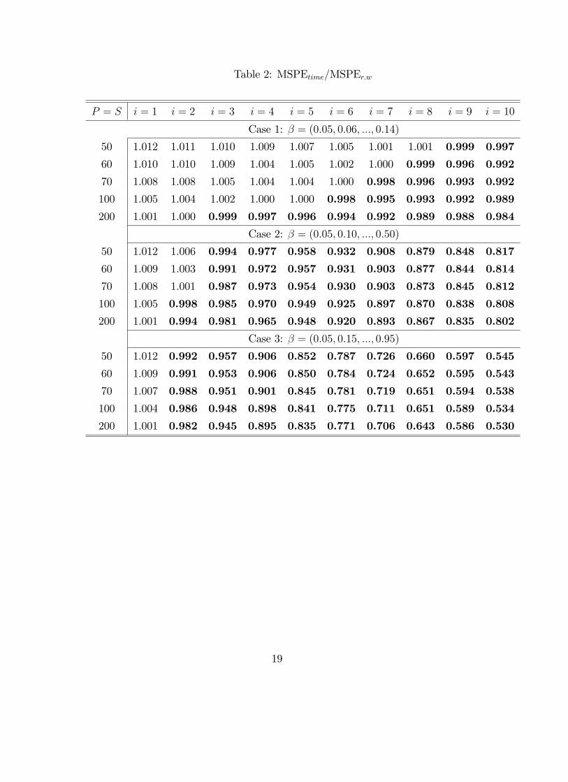
Table 2: MSPEtime=MSPEr:w
P = S i = 1 i = 2 i = 3 i = 4 i = 5 i = 6 i = 7 i = 8 i = 9 i = 10
Case 1: � = (0:05; 0:06; :::; 0:14)
50 1.012 1.011 1.010 1.009 1.007 1.005 1.001 1.001 0.999 0.997
60 1.010 1.010 1.009 1.004 1.005 1.002 1.000 0.999 0.996 0.992
70 1.008 1.008 1.005 1.004 1.004 1.000 0.998 0.996 0.993 0.992
100 1.005 1.004 1.002 1.000 1.000 0.998 0.995 0.993 0.992 0.989
200 1.001 1.000 0.999 0.997 0.996 0.994 0.992 0.989 0.988 0.984
Case 2: � = (0:05; 0:10; :::; 0:50)
50 1.012 1.006 0.994 0.977 0.958 0.932 0.908 0.879 0.848 0.817
60 1.009 1.003 0.991 0.972 0.957 0.931 0.903 0.877 0.844 0.814
70 1.008 1.001 0.987 0.973 0.954 0.930 0.903 0.873 0.845 0.812
100 1.005 0.998 0.985 0.970 0.949 0.925 0.897 0.870 0.838 0.808
200 1.001 0.994 0.981 0.965 0.948 0.920 0.893 0.867 0.835 0.802
Case 3: � = (0:05; 0:15; :::; 0:95)
50 1.012 0.992 0.957 0.906 0.852 0.787 0.726 0.660 0.597 0.545
60 1.009 0.991 0.953 0.906 0.850 0.784 0.724 0.652 0.595 0.543
70 1.007 0.988 0.951 0.901 0.845 0.781 0.719 0.651 0.594 0.538
100 1.004 0.986 0.948 0.898 0.841 0.775 0.711 0.651 0.589 0.534
200 1.001 0.982 0.945 0.895 0.835 0.771 0.706 0.643 0.586 0.530
19

Table 3: MSPEpool=MSPEr:w
P = S i = 1 i = 2 i = 3 i = 4 i = 5 i = 6 i = 7 i = 8 i = 9 i = 10
Case 1: � = (0:05; 0:06; :::; 0:14)
50 1.001 0.999 0.997 0.996 0.993 0.992 0.988 0.988 0.987 0.985
60 1.001 0.999 1.000 0.994 0.993 0.991 0.990 0.988 0.986 0.984
70 1.001 1.000 0.997 0.995 0.994 0.991 0.989 0.987 0.986 0.984
100 1.001 0.999 0.996 0.995 0.993 0.991 0.989 0.987 0.986 0.984
200 1.000 0.998 0.996 0.994 0.992 0.991 0.989 0.987 0.985 0.983
Case 2: � = (0:05; 0:10; :::; 0:50)
50 1.053 1.024 0.998 0.971 0.946 0.920 0.900 0.878 0.860 0.843
60 1.054 1.025 0.996 0.966 0.948 0.921 0.897 0.879 0.859 0.844
70 1.050 1.025 0.994 0.972 0.947 0.922 0.899 0.877 0.860 0.843
100 1.051 1.023 0.996 0.970 0.944 0.919 0.896 0.877 0.857 0.842
200 1.048 1.022 0.994 0.968 0.946 0.918 0.895 0.877 0.858 0.840
Case 3: � = (0:05; 0:15; :::; 0:95)
50 1.215 1.109 1.012 0.917 0.844 0.778 0.728 0.686 0.655 0.637
60 1.204 1.108 1.007 0.921 0.845 0.777 0.728 0.683 0.656 0.637
70 1.204 1.100 1.006 0.915 0.840 0.775 0.726 0.682 0.655 0.635
100 1.207 1.103 1.004 0.914 0.838 0.771 0.721 0.684 0.653 0.634
200 1.203 1.100 1.003 0.914 0.835 0.770 0.719 0.681 0.654 0.633
Table 4
Theil�s U-Statistics: time-series Model
Horizon CAN DEN JAP KOR NOR SWE UK Euro
1 1.083 1.010 1.003 0.982 1.033 1.026 1.022 1.023
2 1.207 1.014 1.001 0.966 1.078 1.067 1.048 1.015
3 1.416 1.012 1.000 0.949 1.133 1.109 1.076 0.995
4 1.675 1.016 1.003 0.937 1.227 1.155 1.113 0.988
5 2.018 1.026 1.002 0.923 1.340 1.215 1.151 0.977
6 2.336 1.046 1.016 0.909 1.448 1.291 1.197 0.977
20

Table 5
Theil�s U-Statistics: Pooled Case
Horizon CAN DEN JAP KOR NOR SWE UK Euro
1 1.014 1.003 0.992 0.974 0.989 1.008 1.098 0.991
2 1.026 0.998 0.978 0.954 0.989 1.014 1.242 0.976
3 1.042 0.998 0.962 0.929 0.988 1.018 1.403 0.960
4 1.065 1.002 0.950 0.916 1.003 1.018 1.566 0.947
5 1.089 1.010 0.936 0.902 1.031 1.015 1.733 0.931
6 1.108 1.024 0.925 0.891 1.057 1.017 1.919 0.918
Table 6
Theil�s U-Statistics: Pooled/time-series and Comparison of Mean Square
Estimation Error
Horizon CAN DEN JAP KOR NOR SWE UK Euro
Theil�s U-Statistics: Pooled/Time Series
1 0.936 0.994 0.990 0.992 0.957 0.983 1.074 0.970
2 0.850 0.985 0.977 0.987 0.918 0.950 1.185 0.962
3 0.736 0.986 0.962 0.979 0.872 0.918 1.304 0.965
4 0.636 0.987 0.946 0.977 0.818 0.881 1.407 0.958
5 0.540 0.984 0.934 0.977 0.769 0.835 1.505 0.953
6 0.474 0.979 0.911 0.981 0.730 0.788 1.603 0.939
Mean Square Estimation Error, P;i1 -0.001 0.000 0.000 0.000 0.000 -0.001 0.000 -0.006
2 -0.008 -0.001 0.000 0.000 -0.002 -0.005 0.001 -0.032
3 -0.026 -0.002 0.000 0.001 -0.004 -0.012 0.001 -0.075
4 -0.055 -0.003 0.001 0.001 -0.008 -0.025 0.002 -0.135
5 -0.104 -0.004 0.002 0.003 -0.014 -0.047 0.004 -0.218
6 -0.168 -0.006 0.004 0.004 -0.021 -0.077 0.006 -0.331
21