Why Crime Doesn’t Pay: Locating Criminals Through ...morrow/mcm/7272.pdf · Why Crime Doesn’t Pay: Locating Criminals Through Geographic Pro ling Control Number: #7272 February

Why Crime Doesn’t Pay: Locating Criminals

Through Geographic Profiling

Control Number: #7272

February 22, 2010

Abstract

Geographic profiling, the application of mathematics to criminology,has greatly improved police efforts to catch serial criminals by finding theirresidence. However, many geographic profiles either generate an extremelylarge area for police to cover or generates regions that are unstable withrespect to internal parameters of the model. We propose, formulate, andtest the Gaussian Rossmooth (GRS) Method, which takes the strongestelements from multiple existing methods and combines them into a morestable and robust model. We also propose and test a model to predictthe location of the next crime. We tested our models on the YorkshireRipper case. Our results show that the GRS Method accurately predictsthe location of the killer’s residence. Additionally, the GRS Method ismore stable with respect to internal parameters and more robust withrespect to outliers than the existing methods. The model for predictingthe location of the next crime generates a logical and reasonable regionwhere the next crime may occur. We conclude that the GRS Method is arobust and stable model for creating a strong and effective model.

1

Control number: #7272 2

Contents

1 Introduction 4

2 Plan of Attack 4

3 Definitions 4

4 Existing Methods 54.1 Great Circle Method . . . . . . . . . . . . . . . . . . . . . . . . . 54.2 Centrography . . . . . . . . . . . . . . . . . . . . . . . . . . . . . 64.3 Rossmo’s Formula . . . . . . . . . . . . . . . . . . . . . . . . . . 8

5 Assumptions 8

6 Gaussian Rossmooth 106.1 Properties of a Good Model . . . . . . . . . . . . . . . . . . . . . 106.2 Outline of Our Model . . . . . . . . . . . . . . . . . . . . . . . . 116.3 Our Method . . . . . . . . . . . . . . . . . . . . . . . . . . . . . . 11

6.3.1 Rossmooth Method . . . . . . . . . . . . . . . . . . . . . . 116.3.2 Gaussian Rossmooth Method . . . . . . . . . . . . . . . . 14

7 Gaussian Rossmooth in Action 157.1 Four Corners: A Simple Test Case . . . . . . . . . . . . . . . . . 157.2 Yorkshire Ripper: A Real-World Application of the GRS Method 167.3 Sensitivity Analysis of Gaussian Rossmooth . . . . . . . . . . . . 177.4 Self-Consistency of Gaussian Rossmooth . . . . . . . . . . . . . . 19

8 Predicting the Next Crime 208.1 Matrix Method . . . . . . . . . . . . . . . . . . . . . . . . . . . . 208.2 Boundary Method . . . . . . . . . . . . . . . . . . . . . . . . . . 21

9 Boundary Method in Action 21

10 Limitations 22

11 Executive Summary 2311.1 Outline of Our Model . . . . . . . . . . . . . . . . . . . . . . . . 2311.2 Running the Model . . . . . . . . . . . . . . . . . . . . . . . . . . 2311.3 Interpreting the Results . . . . . . . . . . . . . . . . . . . . . . . 2411.4 Limitations . . . . . . . . . . . . . . . . . . . . . . . . . . . . . . 24

12 Conclusions 25

Appendices 25

A Stability Analysis Images 25

2


List of Figures

1 The effect of outliers upon centrography. The current spatialmean is at the red diamond. If the two outliers in the lower leftcorner were removed, then the center of mass would be locatedat the yellow triangle. . . . . . . . . . . . . . . . . . . . . . . . . 6

2 Crimes scenes that are located very close together can yield illog-ical results for the spatial mean. In this image, the spatial meanis located at the same point as one of the crime scenes at (1,1). . 7

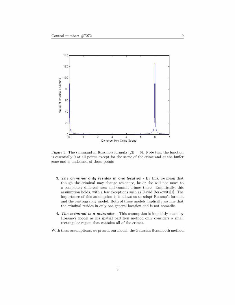
3 The summand in Rossmo’s formula (2B = 6). Note that thefunction is essentially 0 at all points except for the scene of thecrime and at the buffer zone and is undefined at those points . . 9

4 The summand in smoothed Rossmo’s formula (2B = 6, φ = 0.5,and EPSILON = 0.5). Note that there is now a region aroundthe buffer zone where the value of the function no longer changesvery rapidly. . . . . . . . . . . . . . . . . . . . . . . . . . . . . . . 13

5 The Four Corners Test Case. Note that the highest hot spot islocated at the center of the grid, just as the mathematics indicates. 15

6 Crimes and residences of the Yorkshire Ripper. There are tworesidences as the Ripper moved in the middle of the case. Someof the crime locations are assaults and others are murders. . . . . 16

7 GRS output for the Yorkshire Ripper case (B = 2.846). Blackdots indicate the two residences of the killer. . . . . . . . . . . . 17

8 GRS method run on Yorkshire Ripper data (B = 2). Note thatthe major difference between this model and Figure 7 is that thehot zones in this figure are smaller than in the original run. . . . 18

9 GRS method run on Yorkshire Ripper data (B = 4). Note thatthe major difference between this model and Figure 7 is that thehot zones in this figure are larger than in the original run. . . . . 19

10 The boundary region generated by our Boundary Method. Notethat boundary region covers many of the crimes committed bythe Sutcliffe. . . . . . . . . . . . . . . . . . . . . . . . . . . . . . 22

11 GRS Method on first eleven murders in the Yorkshire Ripper Case 2512 GRS Method on first twelve murders in the Yorkshire Ripper Case 26

3


1 Introduction

Catching serial criminals is a daunting problem for law enforcement officersaround the world. On the one hand, a limited amount of data is available to thepolice in terms of crimes scenes and witnesses. However, acquiring more dataequates to waiting for another crime to be committed, which is an unacceptabletrade-off. In this paper, we present a robust and stable geographic profileto predict the residence of the criminal and the possible locations of the nextcrime. Our model draws elements from multiple existing models and synthesizesthem into a unified model that makes better use of certain empirical facts ofcriminology.

2 Plan of Attack

Our objective is to create a geographic profiling model that accurately describesthe residence of the criminal and predicts possible locations for the next attack.In order to generate useful results, our model must incorporate two differentschemes and must also describe possible locations of the next crime. Addi-tionally, we must include assumptions and limitations of the model in order toensure that it is used for maximum effectiveness.

To achieve this objective, we will proceed as follows:

1. Define Terms - This ensures that the reader understands what we aretalking about and helps explain some of the assumptions and limitationsof the model.

2. Explain Existing Models - This allows us to see how others have at-tacked the problem. Additionally, it provides a logical starting point forour model.

3. Describe Properties of a Good Model- This clarifies our objectiveand will generate a sketelon for our model.

With this underlying framework, we will present our model, test it with existingdata, and compare it against other models.

3 Definitions

The following terms will be used throughout the paper:

1. Spatial Mean - Given a set of points, S, the spatial mean is the pointthat represents the middle of the data set.

2. Standard Distance - The standard distance is the analog of standarddeviation for the spatial mean.

4


3. Marauder - A serial criminal whose crimes are situated around his or herplace of residence.

4. Distance Decay - An empirical phenomenon where criminal don’t traveltoo far to commit their crimes.

5. Buffer Area - A region around the criminal’s residence or workplacewhere he or she does not commit crimes.[1] There is some dispute as towhether this region exists. [2] In our model, we assume that the bufferarea exists and we measure it in the same spatial unit used to describethe relative locations of other crime scenes.

6. Manhattan Distance - Given points a = (x1, y1) and b = (x2, y2), theManhattan distance from a to b is |x1−x2|+ |y1−y2|. This is also knownas the 1− norm.

7. Nearest Neighbor Distance - Given a set of points S, the nearestneighbor distance for a point x ∈ S is

mins∈S−{x}

|x− s|

Any norm can be chosen.

8. Hot Zone - A region where a predictive model states that a criminal mightbe. Hot zones have much higher predictive scores than other regions ofthe map.

9. Cold Zone - A region where a predictive model scores exceptionally low.

4 Existing Methods

Currently there are several existing methods for interpolating the position of acriminal given the location of the crimes.

4.1 Great Circle Method

In the great circle method, the distances between crimes are computed andthe two most distant crimes are chosen. Then, a great circle is drawn so thatboth of the points are on the great circle. The midpoint of this great circle isthen the assumed location of the criminal’s residence and the area bounded bythe great circle is where the criminal operates. This model is computationallyinexpensive and easy to understand. [3] Moreover, it is easy to use and requiresvery little training in order to master the technique.[2] However, it has certaindrawbacks. For example, the area given by this method is often very large andother studies have shown that a smaller area suffices. [4] Additionally, a fewoutliers can generate an even larger search area, thereby further slowing thepolice effort.

5


4.2 Centrography

In centrography, crimes are assigned x and y coordinates and the “center ofmass” is computed as follows:

xcenter =n∑i=1

xin

ycenter =n∑i=1

yin

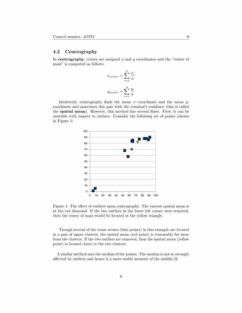
Intuitively, centrography finds the mean x−coordinate and the mean y-coordinate and associates this pair with the criminal’s residence (this is calledthe spatial mean). However, this method has several flaws. First, it can beunstable with respect to outliers. Consider the following set of points (shownin Figure 1:

Figure 1: The effect of outliers upon centrography. The current spatial mean isat the red diamond. If the two outliers in the lower left corner were removed,then the center of mass would be located at the yellow triangle.

Though several of the crime scenes (blue points) in this example are locatedin a pair of upper clusters, the spatial mean (red point) is reasonably far awayfrom the clusters. If the two outliers are removed, then the spatial mean (yellowpoint) is located closer to the two clusters.

A similar method uses the median of the points. The median is not so stronglyaffected by outliers and hence is a more stable measure of the middle.[3]

6


Alternatively, we can circumvent the stability problem by incorporating the2-D analog of standard deviation called the standard distance:

σSD =

√∑dcenter,iN

where N is the number of crimes committed and dcenter,i is the distance fromthe spatial center to the ith crime.

By incorporating the standard distance, we get an idea of how “close together”the data is. If the standard distance is small, then the kills are close together.However, if the standard distance is large, then the kills are far apart.

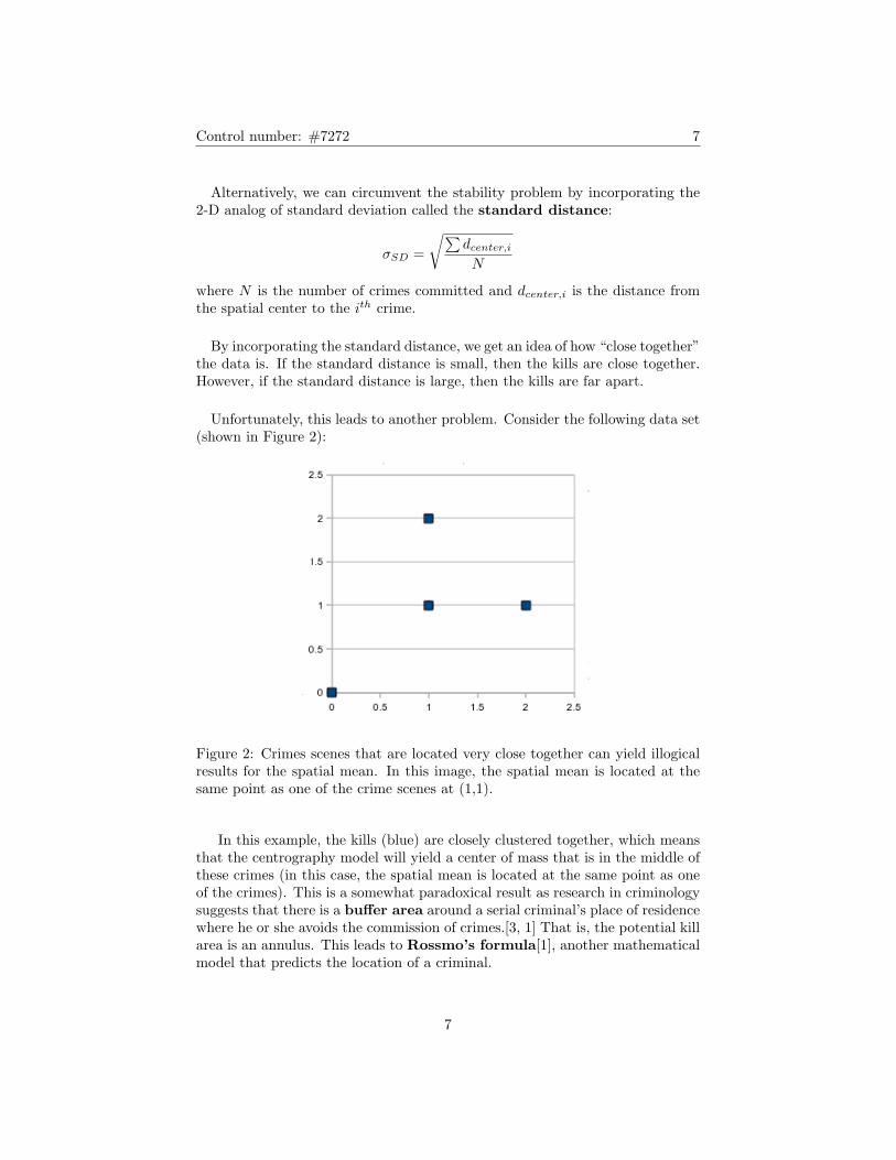
Unfortunately, this leads to another problem. Consider the following data set(shown in Figure 2):

Figure 2: Crimes scenes that are located very close together can yield illogicalresults for the spatial mean. In this image, the spatial mean is located at thesame point as one of the crime scenes at (1,1).

In this example, the kills (blue) are closely clustered together, which meansthat the centrography model will yield a center of mass that is in the middle ofthese crimes (in this case, the spatial mean is located at the same point as oneof the crimes). This is a somewhat paradoxical result as research in criminologysuggests that there is a buffer area around a serial criminal’s place of residencewhere he or she avoids the commission of crimes.[3, 1] That is, the potential killarea is an annulus. This leads to Rossmo’s formula[1], another mathematicalmodel that predicts the location of a criminal.

7


4.3 Rossmo’s Formula

Rossmo’s formula divides the map of a crime scene into grid with i rows and jcolumns. Then, the probability that the criminal is located in the box at row iand column j is

Pi,j = k

T∑c=1

[φ

(|xi − xc|+ |yj − yc|)f+

(1− φ)(Bg−f )(2B − |xi − xc| − |yj − yc|)g

]where f = g = 1.2, k is a scaling constant (so that P is a probability function),T is the total number of crimes, φ puts more weight on one metric than theother, and B is the radius of the buffer zone (and is suggested to be one-half themean of the nearest neighbor distance between crimes).[1] Rossmo’s formulaincorporates two important ideas:

1. Criminals won’t travel too far to commit their crimes. This is known asdistance decay.

2. There is a buffer area around the criminal’s residence where the crimesare less likely to be committed.

However, Rossmo’s formula has two drawbacks. If for any crime scene xc, yc,

the equality 2B = |xi−xc|+|yj−yc|, is satisfied, then the term(1− φ)(Bg−f )

(2B − |xi − xc| − |yj − yc|)gis undefined, as the denominator is 0. Additionally, if the region associated with

ij is the same region as the crime scene, thenφ

(|xi − xc|+ |yj − yc|)fis unde-

fined by the same reasoning. Figure 3 illustrates this:This “delta function-like” behavior is disconcerting as it essentially states

that the criminal either lives right next to the crime scene or on the boundarydefined by Rossmo. Hence, the B-value becomes exceptionally important andneeds its own heuristic to ensure its accuracy. A non-optimal choice of B canresult in highly unstable search zones that vary when B is altered slightly.

5 Assumptions

Our model is an expansion and adjustment of two existing models, centrographyand Rossmo’s formula, which have their own underlying assumptions. In orderto create an effective model, we will make the following assumptions:

1. The buffer area exists - This is a necessary assumption and is the basisfor one of the mathematical components of our model.

2. More than 5 crimes have occurred - This assumption is importantas it ensures that we have enough data to make an accurate model. Ad-ditionally, Rossmo’s model stipulates that 5 crimes have occurred[1].

8


Figure 3: The summand in Rossmo’s formula (2B = 6). Note that the functionis essentially 0 at all points except for the scene of the crime and at the bufferzone and is undefined at those points

3. The criminal only resides in one location - By this, we mean thatthough the criminal may change residence, he or she will not move toa completely different area and commit crimes there. Empirically, thisassumption holds, with a few exceptions such as David Berkowitz[1]. Theimportance of this assumption is it allows us to adapt Rossmo’s formulaand the centrography model. Both of these models implicitly assume thatthe criminal resides in only one general location and is not nomadic.

4. The criminal is a marauder - This assumption is implicitly made byRossmo’s model as his spatial partition method only considers a smallrectangular region that contains all of the crimes.

With these assumptions, we present our model, the Gaussian Rossmooth method.

9


6 Gaussian Rossmooth

6.1 Properties of a Good Model

Much of the literature regarding criminology and geographic profiling containscriticism of existing models for catching criminals. [1, 2] From these criticisms,we develop the following criteria for creating a good model:

1. Gives an accurate prediction for the location of the criminal -This is vital as the objective of this model is to locate the serial criminal.Obviously, the model cannot give a definite location of the criminal, butit should at least give law enforcement officials a good idea where to look.

2. Provides a good estimate of the location of the next crime - Thisobjective is slightly harder than the first one, as the criminal can choosethe location of the next crime. Nonetheless, our model should generate aregion where law enforcement can work to prevent the next crime.

3. Robust with respect to outliers - Outliers can severely skew predic-tions such as the one from the centrography model. A good model willbe able to identify outliers and prevent them from adversely affecting thecomputation.

4. Consitent within a given data set - That is, if we eliminate data pointsfrom the set, they do not cause the estimation of the criminal’s locationto change excessively. Additionally, we note that if there are, for example,eight murders by one serial killer, then our model should give a similarprediction of the killer’s residence when it considers the first five, first six,first seven, and all eight murders.

5. Easy to compute - We want a model that does not entail excessivecomputation time. Hence, law enforcement will be able to get their infor-mation more quickly and proceed with the case.

6. Takes into account empirical trends - There is a vast amount ofempirical data regarding serial criminals and how they operate. A goodmodel will incorporate this data in order to minimize the necessary searcharea.

7. Tolerates changes in internal parameters - When we tested Rossmo’sformula, we found that it was not very tolerant to changes of the internalparameters. For example, varying B resulted in substantial changes in thesearch area. Our model should be stable with respect to its parameters,meaning that a small change in any parameter should result in a smallchange in the search area.

10


6.2 Outline of Our Model

We know that centrography and Rossmo’s method can both yield valuable re-sults. When we used the mean and the median to calculate the centroid of astring of murders in Yorkshire, England, we found that both the median-basedand mean-based centroid were located very close to the home of the criminal.Additionally, Rossmo’s method is famous for having predicted the home of acriminal in Louisiana. In our approach to this problem, we adapt these methodsto preserve their strengths while mitigating their weaknesses.

1. Smoothen Rossmo’s formula - While the theory behind Rossmo’s for-mula is well documented, its implementation is flawed in that his formulareaches asymptotes when the distance away from a crime scene is 0 (i.e.point (xi, yj) is a crime scene), or when a point is exactly 2B away froma crime scene. We must smoothen Rossmo’s formula so that idea of abuffer area is mantained, but the asymptotic behavior is removed and thetolerance for error is increased.

2. Incorporate the spatial mean - Using the existing crime scenes, we willcompute the spatial mean. Then, we will insert a Gaussian distributioncentered at that point on the map. Hence, areas near the spatial meanare more likely to come up as hot zones while areas further away fromthe spatial mean are less likely to be viewed as hot zones. This ensuresthat the intuitive idea of centrography is incorporated in the model andalso provides a general area to search. Moreover, it mitigates the effectof outliers by giving a probability boost to regions close to the center ofmass, meaning that outliers are unlikely to show up as hot zones.

3. Place more weight on the first crime - Research indicates that crimi-nals tend to commit their first crime closer to their home than their latterones.[5] By placing more weight on the first crime, we can create a modelthat more effectively utilizes criminal psychology and statistics.

6.3 Our Method

6.3.1 Rossmooth Method

First, we eliminated the scaling constant k in Rossmo’s equation. As such, thefunction is no longer a probability function but shows the relative likelihood ofthe criminal living in a certain sector. In order to eliminate the various spikesin Rossmo’s method, we altered the distance decay function.

11


We wanted a distance decay function that:

1. Preserved the distance decay effect. Mathematically, this meant that thefunction decreased to 0 as the distance tended to infinity.

2. Had an interval around the buffer area where the function values wereclose to each other. Therefore, the criminal could ostensibly live in asmall region around the buffer zone, which would increase the toleranceof the B-value.

We examined various distance decay functions [1, 3] and found that the func-tions resembled f(x) = Ce−m(x−x0)

2. Hence, we replaced the second term in

Rossmo’s function with term of the form (1− φ)× Ce−k(x−x0)2. Our modified

equation was:

Ei,j =T∑c=1

[φ

(|xi − xc|+ |yj − yc|)f+ (1− φ)× Ce−(2B−(|xi−xc|+|yj−yc|))2

]

However, this maintained the problematic region around any crime scene. Inorder to eliminate this problem, we set an EPSILON so that any point withinEPSILON (defined to be 0.5 spatial units) of a crime scene would have a weightingof a constant cap. This prevented the function from reaching an asymptote asit did in Rossmo’s model. The cap was defined as

CAP =φ

EPSILONf

The C in our modified Rossmo’s function was also set to this cap. This way, thetwo maximums of our modified Rossmo’s function would be equal and would belocated at the crime scene and the buffer zone.

12


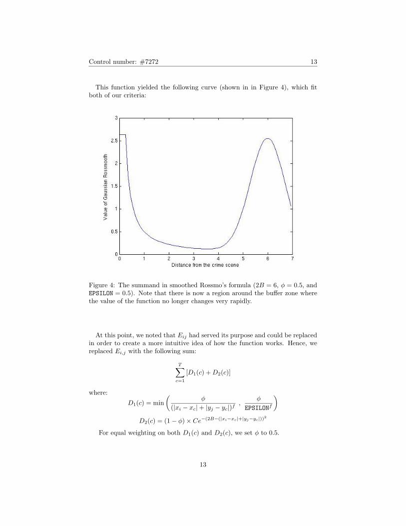
This function yielded the following curve (shown in in Figure 4), which fitboth of our criteria:

Figure 4: The summand in smoothed Rossmo’s formula (2B = 6, φ = 0.5, andEPSILON = 0.5). Note that there is now a region around the buffer zone wherethe value of the function no longer changes very rapidly.

At this point, we noted that Eij had served its purpose and could be replacedin order to create a more intuitive idea of how the function works. Hence, wereplaced Ei,j with the following sum:

T∑c=1

[D1(c) +D2(c)]

where:

D1(c) = min(

φ

(|xi − xc|+ |yj − yc|)f,

φ

EPSILONf

)D2(c) = (1− φ)× Ce−(2B−(|xi−xc|+|yj−yc|))2

For equal weighting on both D1(c) and D2(c), we set φ to 0.5.

13


6.3.2 Gaussian Rossmooth Method

Now, in order to incorporate the inuitive method, we used centrography tolocate the center of mass. Then, we generated a Gaussian function centered atthis point. The Gaussian was given by:

G = Ae−

0@ (x− xcenter)2

2σ2x

+(y − ycenter)2

2σ2y

1A

where A is the amplitude of the peak of the Gaussian. We determined thatthe optimal A was equal to 2 times the cap defined in our modified Rossmo’sequation. (A = 2φ

EPSILONf )

To deal with empirical evidence that the first crime was usually the closest tothe criminal’s residence, we doubled the weighting on the first crime. However,the weighting can be represented by a constant, W . Hence, our final GaussianRosmooth function was:

GRS(xi, yj) = G+W (D1(1) +D2(1)) +T∑c=2

[D1(c) +D2(c)]

14


7 Gaussian Rossmooth in Action

7.1 Four Corners: A Simple Test Case

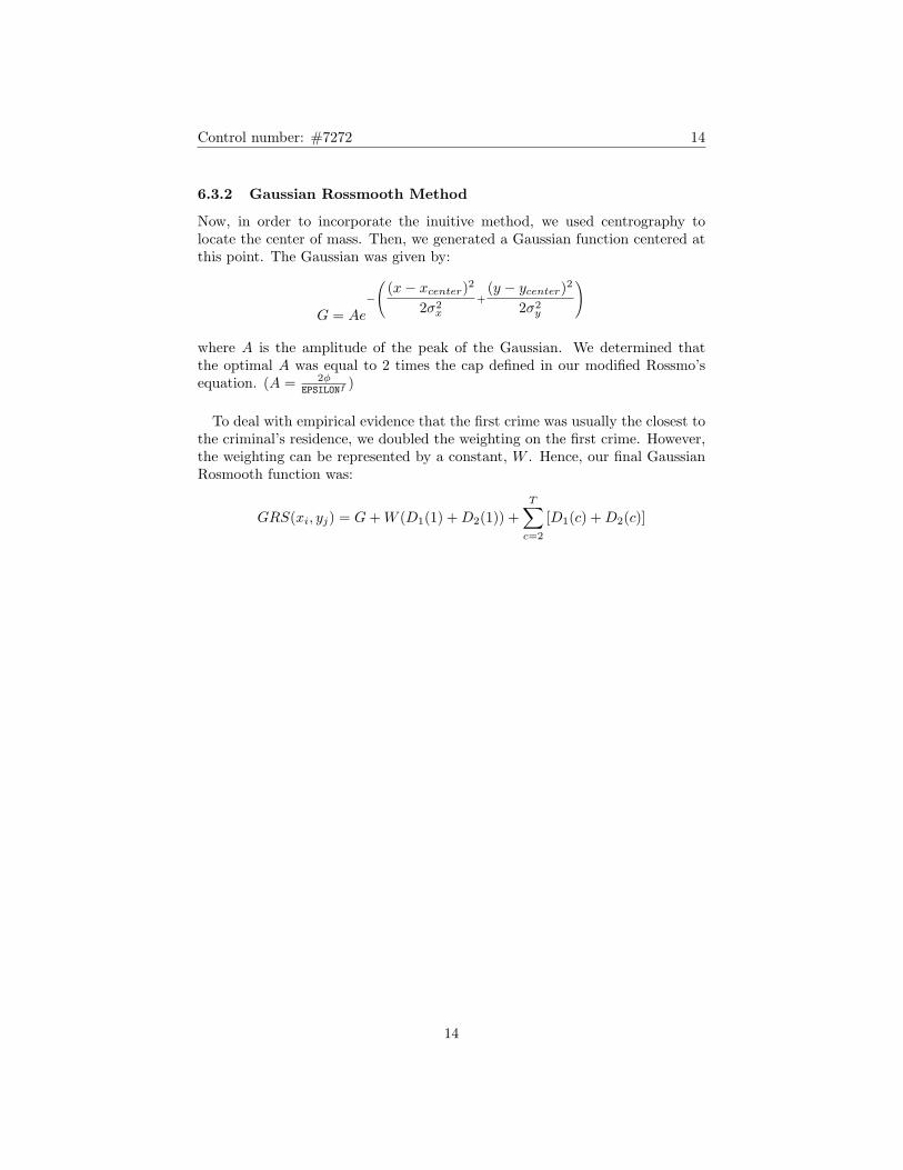
In order to test our Gaussain Rossmooth (GRS) method, we tried it against avery simple test case. We placed crimes on the four corners of a square. Then,we hypothesized that the model would predict the criminal to live in the centerof the grid, with a slightly higher hot zone targeted toward the location of thefirst crime. Figure 5 shows our results, which fits our hypothesis.

Figure 5: The Four Corners Test Case. Note that the highest hot spot is locatedat the center of the grid, just as the mathematics indicates.

15


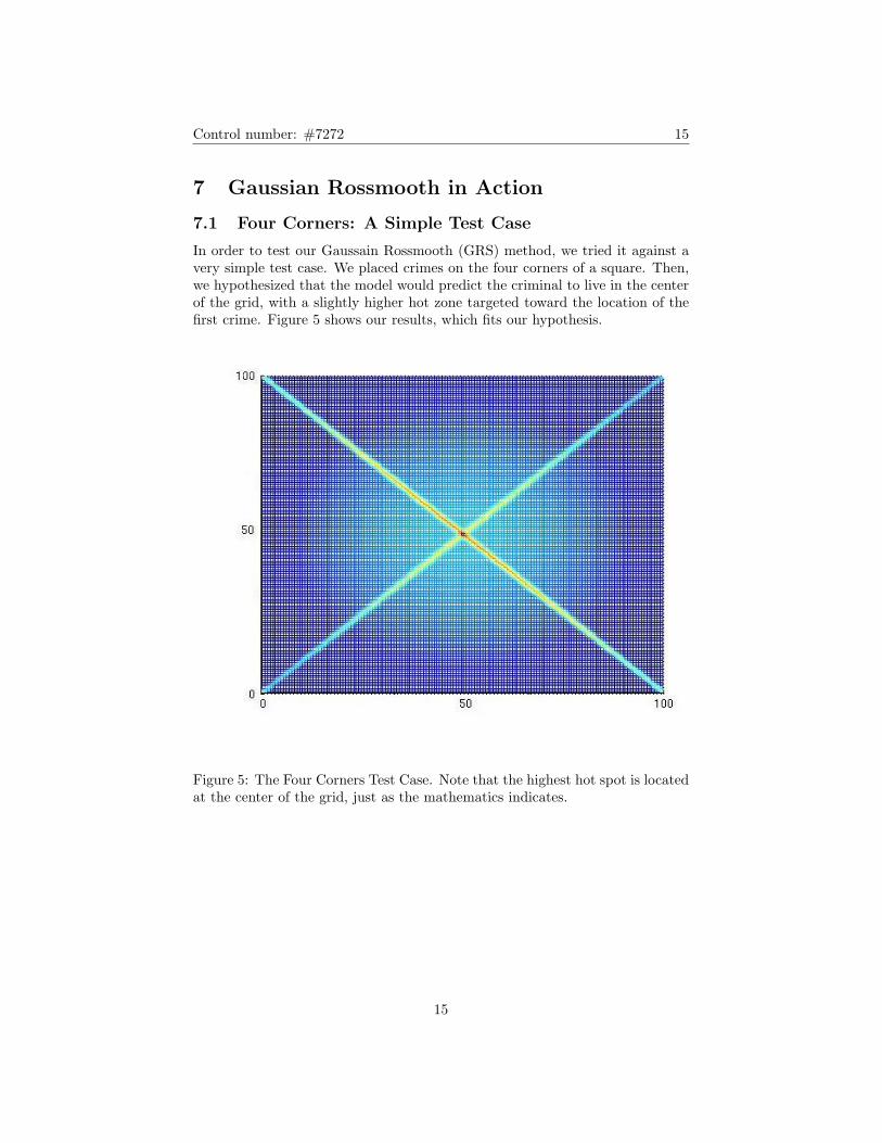
7.2 Yorkshire Ripper: A Real-World Application of theGRS Method

After the model passed a simple test case, we entered the data from the YorkshireRipper case. The Yorkshire Ripper (a.k.a. Peter Sutcliffe) committed a stringof 13 murders and several assaults around Northern England. Figure 6 showsthe crimes of the Yorkshire Ripper and the locations of his residence[1] :

Figure 6: Crimes and residences of the Yorkshire Ripper. There are two res-idences as the Ripper moved in the middle of the case. Some of the crimelocations are assaults and others are murders.

16


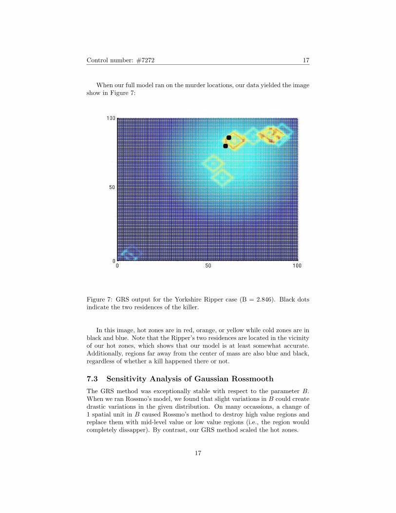
When our full model ran on the murder locations, our data yielded the imageshow in Figure 7:

Figure 7: GRS output for the Yorkshire Ripper case (B = 2.846). Black dotsindicate the two residences of the killer.

In this image, hot zones are in red, orange, or yellow while cold zones are inblack and blue. Note that the Ripper’s two residences are located in the vicinityof our hot zones, which shows that our model is at least somewhat accurate.Additionally, regions far away from the center of mass are also blue and black,regardless of whether a kill happened there or not.

7.3 Sensitivity Analysis of Gaussian Rossmooth

The GRS method was exceptionally stable with respect to the parameter B.When we ran Rossmo’s model, we found that slight variations in B could createdrastic variations in the given distribution. On many occassions, a change of1 spatial unit in B caused Rossmo’s method to destroy high value regions andreplace them with mid-level value or low value regions (i.e., the region wouldcompletely dissapper). By contrast, our GRS method scaled the hot zones.

17


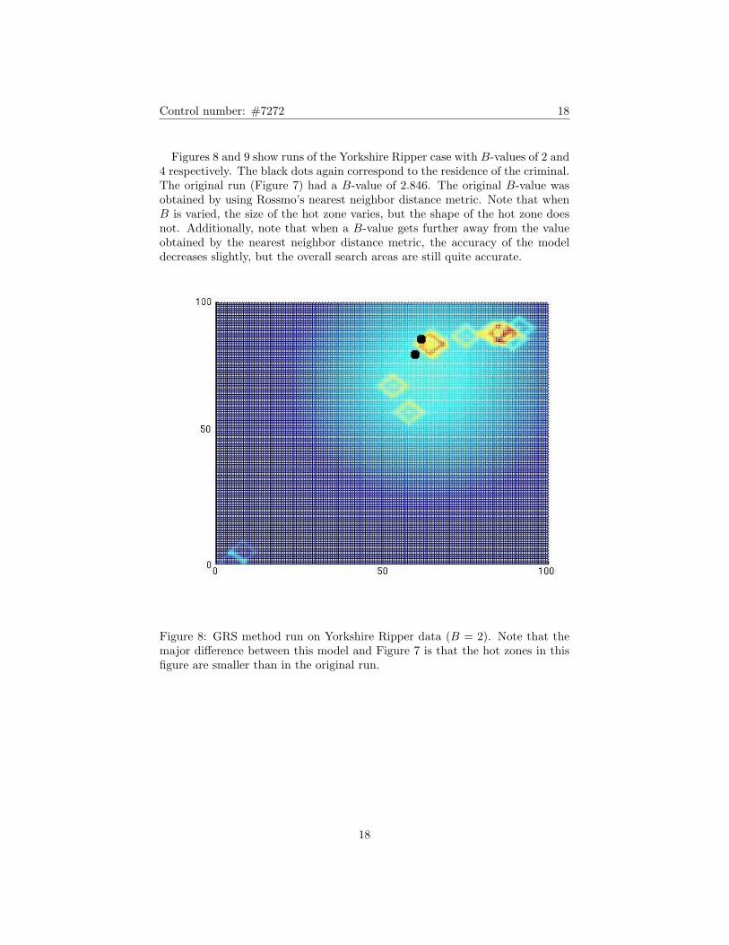
Figures 8 and 9 show runs of the Yorkshire Ripper case with B-values of 2 and4 respectively. The black dots again correspond to the residence of the criminal.The original run (Figure 7) had a B-value of 2.846. The original B-value wasobtained by using Rossmo’s nearest neighbor distance metric. Note that whenB is varied, the size of the hot zone varies, but the shape of the hot zone doesnot. Additionally, note that when a B-value gets further away from the valueobtained by the nearest neighbor distance metric, the accuracy of the modeldecreases slightly, but the overall search areas are still quite accurate.

Figure 8: GRS method run on Yorkshire Ripper data (B = 2). Note that themajor difference between this model and Figure 7 is that the hot zones in thisfigure are smaller than in the original run.

18


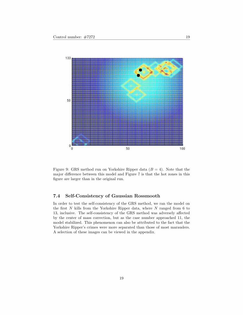
Figure 9: GRS method run on Yorkshire Ripper data (B = 4). Note that themajor difference between this model and Figure 7 is that the hot zones in thisfigure are larger than in the original run.

7.4 Self-Consistency of Gaussian Rossmooth

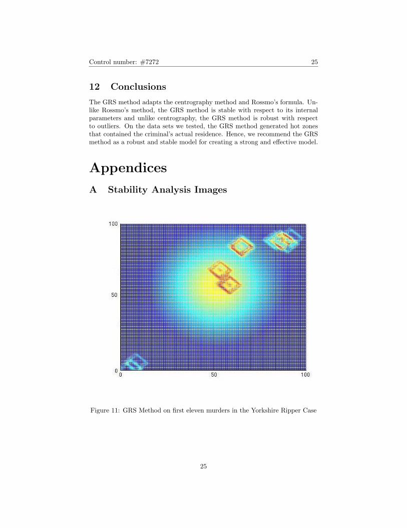
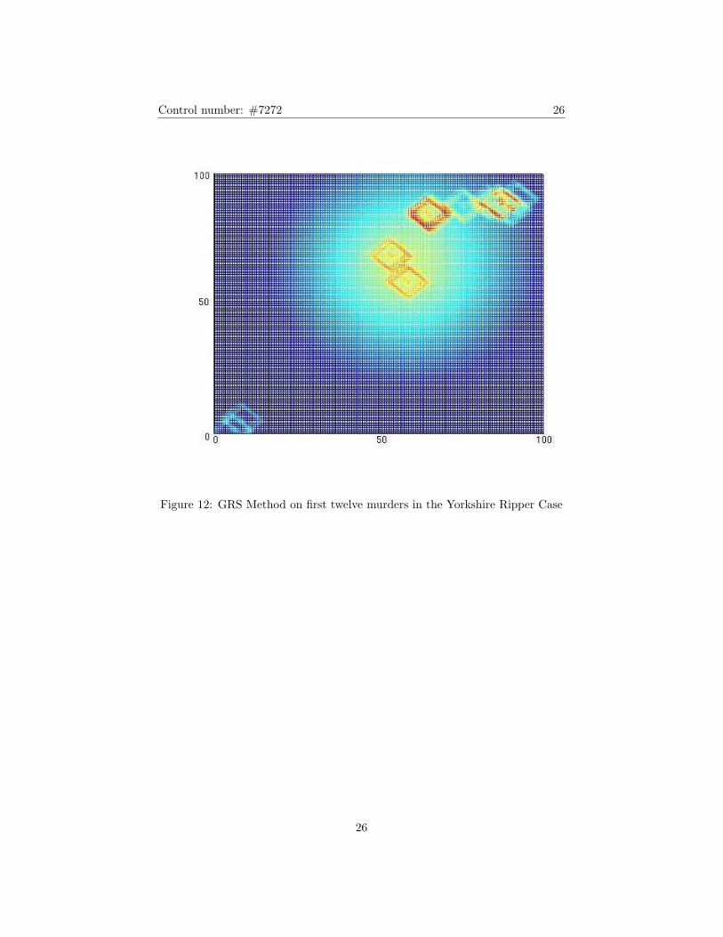
In order to test the self-consistency of the GRS method, we ran the model onthe first N kills from the Yorkshire Ripper data, where N ranged from 6 to13, inclusive. The self-consistency of the GRS method was adversely affectedby the center of mass correction, but as the case number approached 11, themodel stabilized. This phenomenon can also be attributed to the fact that theYorkshire Ripper’s crimes were more separated than those of most marauders.A selection of these images can be viewed in the appendix.

19


8 Predicting the Next Crime

The GRS method generates a set of possible locations for the criminal’s resi-dence. We will now present two possible methods for predicting the locationof the criminal’s next attack. One method is computationally expensive, butmore rigorous while the other method is computationally inexpensive, but moreintuitive.

8.1 Matrix Method

Given the parameters of the GRS method, the region analyzed will be a squarewith side length n spatial units. Then, the output from the GRS method canbe interpreted as an n × n matrix. Hence, for any two runs, we can take thenorm of their matrix difference and compare how similar the runs were. Withthis in mind, we generate the following method.

For every point on the grid:

1. Add crime to this point on the grid.

2. Run the GRS method with the new set of crime points.

3. Compare the matrix generated with these points to the original matrix bysubtracting the components of the original matrix from the componentsof the new matrix.

4. Take a matrix norm of this difference matrix.

5. Remove the crime from this point on the grid.

As a lower matrix norm indicates a matrix similar to our original run, we seekthe points so that the matrix norm is minimized.

There are several matrix norms to choose from. We chose the Frobeniusnorm because it takes into account all points on the difference matrix.[6] TheFrobenius norm is:

||A||F =

√√√√ m∑i=1

n∑j=1

|aij |2

However, the Matrix Method has one serious drawback: it is exceptionallyexpensive to compute. Given an n× n matrix of points and c crimes, the GRSmethod runs in O(cn2). As the Matrix method runs the GRS method at each ofn2 points, we see that the Matrix Method runs in O(cn4). With the YorkshireRipper case, c = 13 and n = 151. Accordingly, it requires a fairly long time topredict the location of the next crime. Hence, we present an alternative solutionthat is more intuitive and efficient.

20


8.2 Boundary Method

The Boundary Method searches the GRS output for the highest point. Then, itcomputes the average distance, r, from this point to the crime scenes. In orderto generate a resonable search area, it discards all outliers (i.e., points thatwere several times further away from the high point than the rest of the crimesscenes.) Then, it draws annuli of outer radius r (in the 1-norm sense) aroundall points above a certain cutoff value, defined to be 60% of the maximum value.This value was chosen as it was a high enough percentage value to contain allof the hot zones.

The beauty of this method is that essentially it uses the same algorithm asthe GRS. We take all points on the hot zone and set them to “crime scenes.”Recall that our GRS formula was :

GRS(xi, yj) = G+W (D1(1) +D2(1)) +T∑c=2

[(D1(c) +D2(c))]

In our boundary model, we only take the terms that involve D2(c). However,let D′2(c) be a modified D2(c) defined as follows:

D′2(c) = (1− φ)× Ce−(r−(|xi−xc|+|yj−yc|))2

Then, the boundary model is:

BS(xi, yj) =T∑c=1

D′2(c)

9 Boundary Method in Action

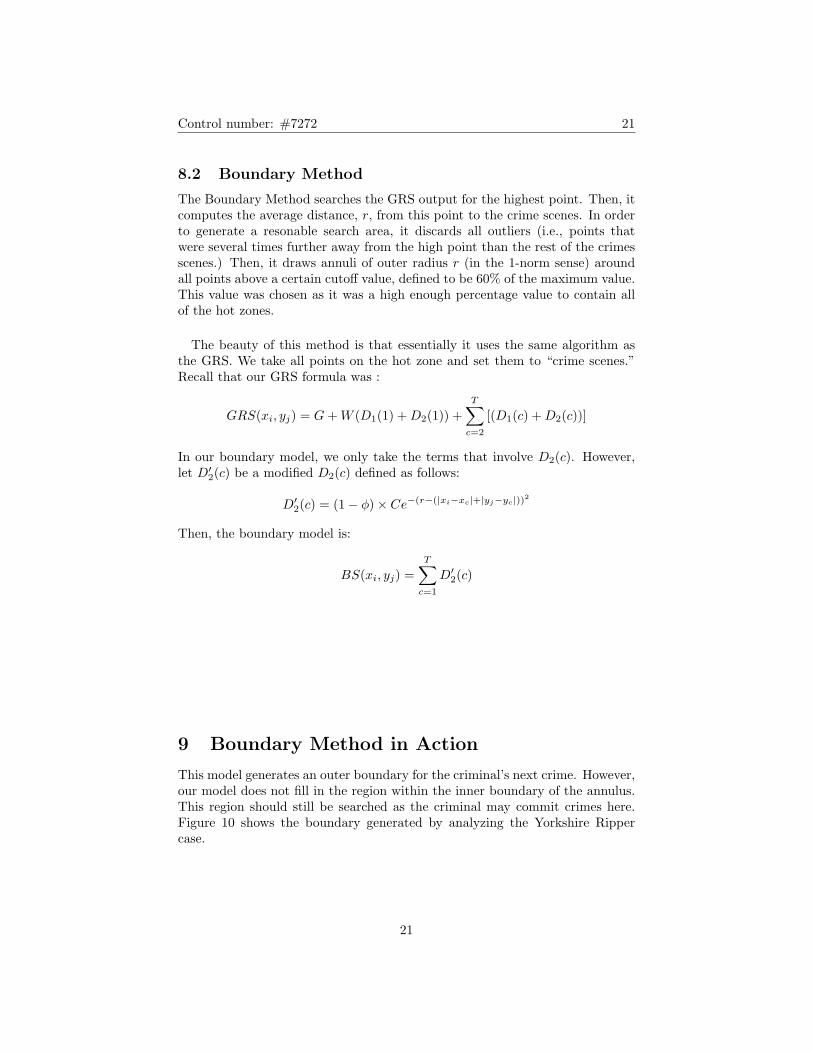
This model generates an outer boundary for the criminal’s next crime. However,our model does not fill in the region within the inner boundary of the annulus.This region should still be searched as the criminal may commit crimes here.Figure 10 shows the boundary generated by analyzing the Yorkshire Rippercase.

21


Figure 10: The boundary region generated by our Boundary Method. Note thatboundary region covers many of the crimes committed by the Sutcliffe.

Even more astonishingly, the boundary method almost perfectly describesthe location of the 12th crime when it is run on the first 11 crimes. The tablebelow shows the highest value predicted locations of crimes scenes and theiractual locations:

Crime # Actual Crime Predicted Crime Distance Difference11 (65, 83) (72, 88) 1212 (75, 87) (72, 88) 413 (84, 88) (78, 84) 10

10 Limitations

Like any predictive model, our model has limitations.

1. There are exceptions to our weighting heuristic - By this, we meanthat some criminals make their first strike far away from home. For ex-ample, Peter Sutcliffe’s first victim was located over 13 miles away fromhis place of residence, much further away from his home than some of his

22


later crimes.[1] Hence, though our model may predict the right location,it can also place hot zones in regions where the criminal does not live.

2. Our model only deals with criminal who are marauders - Somecriminals commit their crimes in a region far away from their place of res-idence. These criminals, known as commuters, will not be so effectivelytracked by our model. However, when we generated the model, we madethe explict assumption that the criminal was a marauder, so if law en-forcement has evidence that the criminal is a commuter, then they shouldkeep that in mind while using our model. (However, Peter Sutcliffe wason the border of commuter and marauder[1], meaning that our model canstill give a surprisingly accurate result.)

11 Executive Summary

Our approach to generating a geographic profile was to combine two existingmodels. We ran our model on test data from the Yorkshire Ripper case and ityielded more precise and accurate estimates of the killer’s two residences thanother existing models. Therefore, our model has been shown to work on realworld data.

11.1 Outline of Our Model

Our model finds points that allow the criminal to reach all crime scenes with thelowest possible total effort. It then factors in the buffer area effect, the tendencyof criminals to avoid committing crimes too close to home. Then, our modelgenerates “hot zones” where the criminal may live. These areas are where policeefforts should start. It also ranks all regions thereby showing were police effortsare probably unnecessary and can be diverted toward other regions.

11.2 Running the Model

Our model requires the input of the locations of crimes. A grid is also requiredso that the crimes can be plotted on that grid. Our model contains severalinternal parameters that can be changed to sharpen the model. Most of theseparameters are set to values that do not need to change from case to case.However, a very important parameter is the buffer area. In order to figure outthe buffer area, find one-half of the average of the nearest neighbor distance ofthe crime scenes. In general, this turns out to be the radius of the buffer area(for murders). For other types of crimes, the B value is smaller.

23


11.3 Interpreting the Results

Our model generates “hot zones”, regions where the criminal may live. The hotzone are ranked on the following scale (from highest to lowest):

1. Red

2. Orange

3. Yellow

4. Green

5. Blue

The higher the value of the zone, the more priority should be given to searchingthis region. Regions with rankings from Red to Yellow should be searched whileregions at or below Green can be avoided until the other regions have beensearched.

In the model for predicting the next crime, we generate a region where thenext crime is likely to occur. This calculation is made by looking at hot zonesand factoring in how far the criminal’s residence is from the location. Theimages created by this model map the outer boundary where a crime is likelyto occur. However, the region inside of this boundary should also be searchedbecause the criminal may change his or her actions due to the increased policepresence.

11.4 Limitations

Our model applies to cases where at least 5 crimes have occurred. The modelcan still be used with fewer than 5 crimes, but it will not be as accurate. Ad-ditionally, our model should be applied when law enforcement believes that thecriminal lives inside of the area bounded by the crimes or near the area wherethe crimes happened. If the criminal lives outside of the region bounded bythe kills, then our model may generate an inaccurate profile. Furthermore, ourmodel doesn’t take terrain into account. When using the model, a human touchis need in order to determine if the model is providing reasonable hot zones.If a hot zone appears in the middle of a body of water or a vast desert, itshould probably be discarded. Likewise, comparing the locations and attributesof other crimes will help narrow down the usefulness of the geographic profile.

24


12 Conclusions

The GRS method adapts the centrography method and Rossmo’s formula. Un-like Rossmo’s method, the GRS method is stable with respect to its internalparameters and unlike centrography, the GRS method is robust with respectto outliers. On the data sets we tested, the GRS method generated hot zonesthat contained the criminal’s actual residence. Hence, we recommend the GRSmethod as a robust and stable model for creating a strong and effective model.

Appendices

A Stability Analysis Images

Figure 11: GRS Method on first eleven murders in the Yorkshire Ripper Case

25


Figure 12: GRS Method on first twelve murders in the Yorkshire Ripper Case

26


References

[1] D. K. Rossmo, Geographic profiling: Target Patterns of Serial Murderers.PhD thesis, Simon Fraser University, 1995.

[2] B. Snook, D. Canter, and C. Bennell, “Predicting the home location of serialoffenders: A preliminary comparison of the accuracy of human judges witha geographic profiling system,” Behavioral Sciences and the Law, 2002.

[3] J. van der Kemp and P. van Koppen, “Fine-tuning geographical profiling,”Criminal Profiling: International Theory, Research, and Practice, 2007.

[4] R. Kocsis and H. Irwin, “An analysis of spatial patterns in serial rape,arson,and burglary: The utility of circle theory of environmental range for psy-chological profiling,” Psychiatry, Psychology, and Law, 1997.

[5] J. Warren, R. Reboussin, R. Hazelwood, and J. Wright, “The geographicaland temporal sequencing of serial rape,” Journal of Interpersonal Violence,1991.

[6] L. W. Johnson and R. D. Riess, Numerical Analysis. Addison-Wesley Edu-cational Publishers Inc, 1977.

27

Documents

Why Crime Doesn’t Pay: Locating Criminals Through ...morrow/mcm/7272.pdf · Why Crime Doesn’t Pay: Locating Criminals Through Geographic Pro ling Control Number: #7272 February