Why do HMOs spend less?Patient selection, physician price sensitivity, and prices∗

Daniel W. Sacks

September, 2018

Abstract

Cost-control incentives have become an important part of the health insurance landscape inthe United States. These incentives are strongest in capitated managed care organizations,especially HMOs, because such organizations are paid a fixed amount regardless of the spendingthey generate. Using a sample of insurance claims from about 500 plans, I find that in HMOs,spending on anti-cholesterol drugs is 19% lower than in other insurance plans. This spendingdifference could reflect the strong cost-control incentives generated by capitation, but it couldalso reflect the selection of healthy, price-sensitive patients into HMOs, or it could simply reflectlower prices. To understand the difference, I estimate a model of physician prescribing andpatient refill decisions. Patients in HMOs are nearly twice as sensitive to copays as are otherpatients, consistent with selection of healthy patients into HMOs. Even after adjusting for thisselection, however, HMO physicians remain highly sensitive to drug procurement costs. Thishigh sensitivity explains about a 20% of the spending difference; combined with lower prices,it explains about 25-55% of the difference. I find no evidence that these spending reductionsresult in fewer patient refills or the prescribing of less effective statins.

JEL codes: G22,I11, I13

∗Kelley School of Business, Indiana University. email: dansacks@indiana.edu. Phone: 812-855-7425. Address:1309 E 10th Street, Bloomington, IN 47405. This paper is a substantially revised version of the first chapter of mydissertation, and it has benefitted enormously from regular discussions with my committee, Mark Duggan, Jean-Francois Houde, Bob Town, and especially Uli Doraszelski and Katja Seim. I am grateful to Susan Lu and ColleenCarey for conference discussion and to Dr. Stephen Gottlieb and Dr. Sarah Miller for providing helpful detail aboutprescribing anti-cholesterol drugs, and to many others too numerous to thank individually for helpful commentsand suggestions. Finally I thank the editor and an unusually patient and helpful referee, whose detailed commentsimproved the paper. This material is based upon work supported by the National Science Foundation GraduateResearch Fellowship under Grant No. DGE-0822219. All errors are my own.

1 Introduction

Cost-control incentives for provider organizations have become an important part of the United

States health care system. The Affordable Care Act helped create Accountable Care Organizations,

which are eligible to profit from any cost savings they generate for Medicare or for private insurers

(McClellan et al., 2010). Medicare has begun experimenting with bundled payments for care,

which entail a fixed payment per episode of care regardless of spending incurred in that episode

(see, e.g., Cassidy (2015)). Both these programs break the link between spending and payment

in traditional, fee-for-service payment systems, and generate incentives for providers to economize

on care and reduce costs. These incentives are similar to those created by capitated payments to

Health Maintenance Organizations (HMOs), in which the HMO is paid a fixed amount per enrollee,

regardless of the care the enrollees use. Indeed, the number of Medicare beneficiaries enrolled in

HMOs doubled (Jacobson et al., 2017). The literature has found that HMOs have lower spending

than other plans, not because they use less care but because they use lower priced care (Cutler et

al., 2000; Altman et al., 2003), in part because treatment decisions in HMOs are particularly price

sensitive (Ho and Pakes, 2014; Dickstein, 2015; Limbrock, 2011).

The existing literature, however, does not distinguish between two competing explanations for

this high price sensitivity: that capitation induces high provider price sensitivity, or that highly

price sensitive patients select into HMOs. This selection is likely because HMOs offer low premiums

in exchange for restrictions on care, and this bargain is likely to be particularly appealing to patients

who would use less care anyway (Glied, 2000). Past literature has addressed selection by including

detailed controls for health status, but not by allowing patient price sensitivity to differ with HMO

status, thus leaving open the possibility that high price sensitivity in HMOs reflects patient selection

and not the effect of provider cost-control incentives.

In this paper, I develop and implement an approach for estimating separate patient and provider

price sensitivities, by HMO status. Separating the two is critical for understanding how the growth

in provider cost-control incentives will affect health care spending. If most of the observed differ-

ential HMO price sensitivity reflects patient selection, then moving towards greater capitation will

have little effect on overall spending. HMO price sensitivity is particularly important in light of

the recently documented enormous variation in health care prices in a given market (Cooper et

al., 2015); if capitated payments to providers induce high price sensitivity, then they might be an

effective tool for directing patients towards low-price, high-value care.

1

To separate patient and provider price sensitivity, I study the demand for prescription drugs,

where physicians write an initial prescription, which patients choose whether to refill. I use these two

separate decisions to separately identify provider and patient price sensitivity. I study prescription

drugs because this is the only health care context in which we observe separate decision making by

physicians and patients, which is critical for separating physician and patient price sensitivity. My

focus is the market for statins, the main class of anti-cholesterol drugs. Statins are among the most

widely used drugs, and spending on them is high. For example, Americans spent nearly $20 billion

on over 260 million prescriptions for statins in 2011 (IMS, 2012). Statins reduce the risk of heart

attack or stroke by about a third (Baigent et al., 2005), but obtaining these health benefits requires

regular refills, since statins treat but do not cure high cholesterol. Statins offer a useful laboratory

for examining cost-control behavior because over time many statins have lost patent protection,

and so very low-price options have gradually become available. Physicians can therefore reduce

spending on statins by substituting generics for patent-protected drugs, but whether they do so

depends on their price sensitivity and their patients’ health needs.

I use data from the MarketScan Databases, which contain health insurance claims data from

about 100 large companies from 1997-2008. I select a sample of nearly 500,000 people in about 500

insurance plans, who are at risk for heart disease and newly prescribed statins. Spending on statins

is lower in HMOs than in other plans, by about $95 per patient, or 19 percent. This difference

is largely due to differential prescribing patterns, rather than differences in refill rates or retail

prices faced. For example, patients in HMOs receive cheaper drugs; on average, their prescribed

drug costs about 19% lower than patients in non-HMOs. This low price largely reflects the fact

that HMO physicians are more than twice as likely as other physicians to prescribe generic drugs.

HMO physicians are also much more likely to prescribe “preferred” drugs, i.e. drugs on the lowest

tier of a formulary. When patients purchase such drugs, insurers often receive rebates from drug

manufacturers (Federal Trade Commission, 2005; Scott Morton and Boller, 2017), so differential

prescribing patterns in HMOs also potentially reflect high physician sensitivity to insurer spending.

However, they could also reflect the selection into HMO of healthy patients, who do not require the

more potent branded drugs and may be especially responsive to the low copays of preferred drugs.

Indeed, patients in HMOs in my data are healthier: they are younger, and less likely to have a

history of heart disease or hypertension.

Healthy patients likely have not only a lower level of demand for health care, but also a greater

price sensitivity of demand for health care, as I show in a simple model. The intuition for this

2

result is that price sensitivity is the inverse of marginal willingness to pay for health improvements

(such as a cholesterol reduction). As patients get healthier, marginal health improvements produce

a smaller benefit, so price sensitivity rises. This result is important because it implies that the high

observed price sensitivity in HMOs could be due not to capitation or physician price sensitivity,

but to selection of healthy patients into these plans.

To decompose the HMO spending difference into physician price sensitivity, patient preferences,

and differential drug prices, I develop a structural empirical model of physician-patient interactions

that allows for selection of healthy, price sensitive patients into HMOs. Physicians write a pre-

scription, and patients decide each month whether to refill it. Patients refill their prescription if

the prescribed drug’s copay is less than its utility, the perceived health benefit of the drug net of

its side effects. Because HMOs may attract healthy or low income patients who do not value drug

quality highly, I allow for the copay sensitivity to differ by HMO status. I use patient refill decisions

to estimate patient copay sensitivity and patient drug preferences. I then estimate physician price

sensitivities using initial prescription choices, but controlling for estimated patient preferences.

I find clear evidence of selection into HMOs. HMO patients are nearly twice as sensitive to their

drug’s copay as non-HMO patient. This is consistent with both healthy people and low-income

people being particularly likely to enroll into HMOs, as these groups are likely to have lower

willingness-to-pay for health care. After adjusting for this selection, I find that HMO physicians re-

main sensitive to drug prices; non-HMO physicians do not respond to prices at all. HMO physicians

are also uniquely sensitive to drug preferredness; the model estimates imply that, all-else-equal,

HMO physicians are 16 percentage points more likely to prescribe a preferred drug.

Even adjusting for the selection of healthy, price sensitive patients into HMOs, HMO physicians

appear uniquely sensitive to drug procurement costs. To quantify the the importance of this

sensitivity for insurer spending, I simulate how prescribing and spending would change if all patients

had physicians with the price and preferredness sensitivity of HMO physicians. The price of the

prescribed drug would fall by about five percent and the probability of receiving a preferred drug

would rise by over a third. These changes would lower statin spending by about $20 per patient

per year ignoring rebates, or $25-$30 per year under reasonable assumptions about the magnitude

of rebates for preferred drugs. This difference is about a quarter of the HMO spending differential.

Lower prices and, especially, increased use of formularies account for an important fraction of

the HMO spending differential. If non-HMOs also used the same formularies and faced the same

prices as HMOs, the spending differential would fall by about three quarters. These spending

3

reductions come without a fall in the refill rates, and with only a trivial change in the strength of

the prescribed drugs, largely because the available generic and preferred statins (to which HMO

physicians substitutes) are effective substitutes for on-patent drugs. Therefore, at least for statin

prescribing, HMOs induce cost-sensitive prescribing without compromising patient health.

I focus on statins because they let me cleanly separate patient and provider preferences. However

the findings here are by necessity specific to statin treatment choice and may not generalize to other

to other contexts. In particular, statins are unusual because there are many options which differ

in price, with relatively little differentiation in terms of quality. Thus, statin prescribing may be

unusually price sensitive (as there is little differentiation), and price sensitivity comes at a low

health cost, relative to other treatments with a more substantial price-quality tradeoff.

This paper primarily contributes to the literature on the effects of managed care and capitation.

Managed care plans attract healthier enrollees, use less health care, and likely reduce costs relative

to traditional insurance (Glied, 2000). One way HMOs reduce spending is through cost-control

incentives for physicians, such as bonuses for meeting spending targets. Using detailed data from a

single capitated managed care organization, Gaynor et al. (2004) provide clear evidence that such

incentives can reduce spending. Managed care reduces spending through lower unit prices, rather

than reductions in quality or quantity of care, as Cutler et al. (2000) show in their study of heart

attack patients. Looking at a wider set of conditions, Altman et al. (2003) decompose the HMO

spending differential into better patient health (which accounts for half), and lower prices (which

accounts for the other half). These papers do not directly estimate price sensitivity, however, nor do

they control for the possibility that low prices of chosen treatment could reflect patient preferences

rather than cost control incentives.1

This paper is most closely related to a series of recent papers by Ho and Pakes (2014), Dickstein

(2015), and Limbrock (2011), which estimate how price sensitivity differs with capitation status. Ho

and Pakes (2014) study hospital referrals for births. After carefully controlling for patient health, Ho

and Pakes find that patients and physicians in more capitated insurers are more willing to tradeoff

distance for price. This willingness-to-travel could reflect high price sensitivity of physicians in

capitated insurers, but it could also reflect patient selection into HMOs, if patients in HMOs have

relatively low time or travel costs.

1A separate literature examines managed care in Medicaid. Duggan (2004) and Duggan and Hayford (2013) findno evidence that Medicaid managed care reduces spending; if anything, it appears to increase spending. It also doesnot improve health; Aizer et al. (2007) find that Medicaid reduces the quality of prenatal care and increases theincidence of low birth weight and infant mortality. Managed care appears to have very different effects in Medicaidthan in the private sector.

4

Dickstein (2015) studies how capitation affects antidepressant prescription choice. He estimates

a logit model of drug demand, allowing for treatment patterns to vary flexibly with capitation

status, but not distinguishing between patient and physician preferences. Prescription choice in

capitated HMOs is more price sensitive, and HMO physicians are more likely to prescribe drugs

which require little follow-up care (for which the physician is not compensated on the margin).

Simulations suggest that switching all patients to a capitated HMO would increase the generic

share by 10 percentage points. Limbrock (2011) studies statin prescribing decisions using one year

of data from the MarketScan Databases. He also shows that HMO physicians are especially likely

to prescribe their plan’s preferred drug even after accounting for selection of high copay-sensitivity

patients into HMOs, and adjusting for age and sex difference by HMO status. However, Limbrock

does not directly estimate price sensitivities, nor does he let patient drug preferences differ between

HMOs and other plans.

The existing literature therefore does not fully separate patient selection—especially on price

sensitivity—and physician price sensitivity in explaining HMO treatment choices. I find that HMO

patients are indeed more price sensitive than are other patients. Even accounting for this difference,

however, I also find that HMO physicians are much more sensitive to drug costs than are other

physicians. Although I cannot identify the exact mechanism behind this greater price sensitivity,

it likely reflects a combination of explicit, physician-level incentives to reduce costs, and implicit

pressure from the HMO to reduce spending. The higher price sensitivity in HMOs accounts for a

substantial share of the HMO spending differential, at least in the context of statins.

2 Institutional background

2.1 Background on statins

I study statins, the main class of anti-cholesterol drugs. There are six statin molecules (i.e.

active ingredients), listed in Table 1, along with two products that combine statins with other

anti-cholesterol drugs; these eight products form the choice set in my analysis. The table reports

the modal dosage of each molecule in my sample and the cholesterol reduction of that dosage,

as estimated in clinical trials.2 This cholesterol reduction is a sufficient statistic for the health

benefits of taking the drug (Baigent et al., 2005), although the side effects may also be worse for

2For simplicity, I refer to each molecule by its trade name rather (e.g. Zocor rather than simvastatin). However Itreat generic and branded versions of the same molecule as the same product substitutes.

5

more powerful drugs. The most powerful drugs are the newest molecules, Lipitor and Crestor; the

older molecules Mevacor, Pravachol, and Zocor, are weaker. Older drugs are also cheaper, as they

have lost patent protection—Mevacor in 2001 and Pravachol and Zocor in 2006.

The prescribing of statins during my sample period follows guidelines laid out by the the Na-

tional Cholesterol Education Program (Gundry et al., 2001). As cholesterol reduction is important

for preventing heart attacks, the guidelines tie prescribing rules to heart disease risk factors. If a

patient has high enough cholesterol given his heart disease risk factors, and if lifestyle intervention

fails, then physicians should prescribe an anti-cholesterol drug. Some of the risk factors are observed

in the claims data: diabetes, hypertension, heart disease, or age related risk. The unobserved risk

factors are smoking and a family history of heart disease. A patient may be prescribed a statin even

if his cholesterol level appears healthy. For example, the guidelines recommend that a 55 year-old

man with diabetes and hypertension be prescribed a statin even if his cholesterol level is below

100, which would be a healthy level for a person with no risk factors. After a drug is prescribed,

the report recommends that the patient continue taking it indefinitely, as high cholesterol is a

chronic condition which statins manage but do not cure. This fact is critical for my interpretation

of refilling: failing to refill the medication—ceasing treatment—does not indicate a cure, and may

indicate dissatisfaction.

2.2 Managed care, capitation, and cost-control incentives

The term “managed care” refers to a broad array of health insurance arrangements.3 In all cases,

an insurer or employer contracts with a managed care organization, which takes an active role in

coordination and managing patient care, and hires physician groups or forms physician networks.

Typically the managed care organization places restrictions on care—for example, precertification

requirements, reviews of physician utilization, and active case management of high cost patients.

These restrictions may make it more difficult for patients to use expensive health care, such as high

cost drugs or hospitals. In exchange for these restrictions, patients may receive a broader set of

benefits (such as dental or vision coverage), and face lower premiums and reduced cost sharing.

In addition to explicitly controlling spending through care restrictions, managed care orga-

nizations can also influence spending by giving their physicians cost-control incentives, including

incentives to reduce drug spending. For example, Gaynor et al. (2004) describe one HMO that pays

its physicians a bonus based on whether they and their colleagues keep spending below a target.

3Glied (2000) provides a valuable overview on managed care plans and the early research on them.

6

Gold et al. (1995) find in a nationally representative survey of managed care organizations that

84 percent had some form of risk sharing with primary care physicians. In a survey in California,

Grumbach et al. (1998) found that in 87 percent of independent physician practices, physicians

were at financial risk for some type of medical care, and of these, 48 percent were at risk for

prescription drugs. In the 2004-2005 Community Tracking Survey, 82 percent of HMO physicians

reported eligibility for some form of incentive payment tied to the performance of their practice

or their individual patients, relative to 46 percent of other physicians (Center for Studying Health

Systems Change, 2008).

Managed care organizations themselves differ in the strength of the cost-control incentives they

face. In some case, the organization is responsible for management but bears very little risk,

passing costs through to an insurer or employer (for self-insured firms). In other cases, however,

the organization bears all or nearly all the risk. This occurs in particular when the organization

is paid on a fully capitated basis: it receives a fixed payment from the insurer per member, and

is responsible for the spending its patients generate. Some managed care contracts “carve out”

particular services (e.g. mental health), for which the insurer (or a third party) bears all risk. In

my data, HMOs are fully capitated managed care organizations, meaning that the insurer does not

pay on the margin for any care; the HMO and the physicians it contracts with bear all the risk.

This is roughly consistent with national patterns for HMOs, which are much more likely to be at

risk for spending than are other managed care organizations.On average, physicians in HMOs say

that 63 percent of their practice revenue is from capitation, versus 11 percent for other physicians

(Center for Studying Health Systems Change, 2008). Likewise, 22 percent of HMO physicians say

that all of their practice revenue is from capitation, versus less than 1 percent of other physicians.

As the incentive for a managed care organization to control spending is strongest in fully capi-

tated HMOs, I am particularly interested in behavior of physicians in these plans. Unfortunately

I do not observe physicians’ contracts with HMOs.4 Observed differences between HMO physi-

cians and other physicians likely represent a combination of explicit HMO control and physicians’

responses to their own financial incentives to keep costs down. I therefore interpret observed dif-

ferences between HMO physicians and other physicians as the effect of capitation payments to the

HMO, rather than the effect of any particular physician incentive scheme.

4Recent papers on capitation and spending share this limitation (e.g. Limbrock (2011); Ho and Pakes (2014);Dickstein (2015)).

7

2.3 Drug pricing, formularies, and rebates

Drug prices are determined jointly by insurers, pharmacies and manufacturers. Insurers de-

termine how much patients pay for drugs by setting copayment rates. They often use a tiered

formulary, in which most generics have one copay, preferred branded drugs have a higher one, and

all other branded drugs have a still higher copay. Insurers pay a retail price to the pharmacy, net

of any copay. This retail price may differ across pharmacies, drugs, and insurers, because phar-

macy prices reflect retailer market power, insurer-retailer negotiations, and drug specific quality

and differentiation (which determine wholesale costs). The price the insurer pays to the pharmacy

is not necessarily the insurer’s true procurement cost, however, because the insurer may receive a

rebate from the drug manufacturer. Manufacturers offer these rebates to insurers in exchange for

including drugs on the formulary or placing them on lower tiers, or for generating large quantities

(Federal Trade Commission, 2005; Scott Morton and Boller, 2017). In a survey of insurers and

pharmacy benefit managers, Federal Trade Commission (2005) found that insurers offered rebates

of up to 27 percent in exchange for preferred tier placement.

These rebates present two challenges for understanding the HMO spending differential. First,

they contribute directly to the differential, because HMOs may be especially likely to benefit from

rebates: HMOs are more likely to use formularies (as I show below) and HMO’s greater control of

physicians may mean that they can more easily encourage physicians to prescribe drugs with large

rebates. Second, if rebates are larger for drugs on the preferred formulary tier, then rebates are

correlated with patient copayment, making it difficult to separately identify physician sensitivity

to rebates (or insurer costs) from physician sensitivity to copayment. In the empirical analysis, I

account for rebates in two steps. First, I identify drugs on the preferred tier of the formulary, and

let physicians have a special preference for these drugs. This accounts for the rebate-copayment

correlation (so that copayment sensitivity is identified from within-tier copay variation.) Second,

when I simulate spending, I allow for large rebates for preferred drugs. In particular, I simulate

spending assuming that insurers receive a 0, 15 or 30 percent rebate on preferred drugs. Although

exact rebate amounts are considered trade secrets, this likely captures the range of possible amounts

and provides some insights into how important rebates are quantitatively for HMO spending.

8

3 The MarketScan Databases

I use data from the Thompson-Reuters MarketScan Databases, in particular the Benefit Plan

Design database and the Commercial Claims and Encounters database. The Benefit Plan Design

database contains detailed information about plan benefit and design for insurance plans in about

100 large companies from 1996 to 2009. The Commercial Claims and Encounters database con-

tains all inpatient, outpatient, and prescription drug claims for these companies, as well as some

demographic information on their enrollees.

3.1 Insurance plan type and managed care features

I use the Benefit Plan Design Database to infer plan type, as well as the presence of managed

care features. To construct this database, MarketScan categorizes information reported in each

plan’s benefit guide, including plan type. These types include comprehensive plans and consumer

directed health plans, which are not managed care plans, as well as four types of managed care plans:

preferred provider organizations (PPO), exclusive provider organizations (EPO), partially capitated

point-of-service plans, and HMOs, which are the only fully capitated plans in the MarketScan

database. That is, among HMO enrollees in my data, the insurer pays for health care only by

making a capitation payment to the HMO. The HMO and not the insurer or the employer is

responsible for all spending. In the empirical analysis, I compare HMOs to all other plans, because

HMOs have the strongest cost-control incentives.

In addition to broad categorizations of plan type, the Benefit Plan Design file also reports the

presence of explicit managed care tools. In particular, there are flags if the benefit guide reports

that the plan has utilization review, case management, or precertification requirements. Appendix

Table D.1 shows the frequency of these tools among fully capitated HMOs, other managed care

plans, and non-managed care plans. Fully capitated HMOs are especially likely to use utilization

review, but they are roughly equally likely to use case management as other plans, and less likely

to use precertification requirements than other managed care plans.5 Although HMOs may pass

on explicit financial incentives to their physicians to control costs, I do not observe these incentives

in my data. I will show, however, that HMO prescribing behavior is uniquely price sensitive,

and remains so even after accounting for the higher prevalence of utilization review. I therefore

interpret this high price sensitivity as the effect of capitation payments to the HMO, although I

5The difference in utilization review between HMOs and other managed care plans is statistically significant, asis the difference in precertification requirements, but the difference in case management is not significant.

9

cannot separate the effects of physician financial incentives from explicit control by the HMO.

3.2 Patient heart disease risk and health

I infer patient heart disease risk factors from the claims and demographic data. I use the full

set of claims to measure past diagnoses of heart disease, diabetes, hypertension, and cholesterol

disorders.6 Following Gundry et al. (2001), I define a person as at risk for heart disease if they

have one of these conditions, or if they are a man 55 or older, or a woman 45 or older. I also use

these data to create several measures of patient health. I construct dummy variables for each of

these conditions, as well as dummy variables for a Charlson comorbidity index of one or at least

two (Charlson et al., 1987).7

3.3 Drug copays, formularies, and prices

I use the payment on the claims to define drug copays and prices. For each insurer, plan-year,

and drug, I define the copay as the average out-of-pocket payment per days’ supply.8 This approach

means that I essentially empirically determine formularies. These formularies differ across insurance

plans, so that the relative copay of two drugs can be quite different, even for plans with similar

overall generosity. Table 2 illustrates this variation for four insurance plans in 2004. In Plans 1 and

2, the overall average copay is about $0.50 per day, but there is clear variation around this average.

In Plan 1, all drugs except the generic Mevacor cost about $0.50 per day, but in Plan 2, Lipitor,

Pravachol, and Crestor are on the preferred tier and Zocor is not. Plans 3 and 4 are less generous

than Plans 1 and 2, with average copays of $1.10, but they also show considerable copay variation

around this average. For example Zocor is on a low tier in Plan 3 but not in Plan 4, where its

copay is nearly twice as high. The relative price of drugs can differ substantially from plan to plan,

even holding fixed overall generosity.9 I define the insurer’s prices similarly to how I define copays.

I start by defining the insurer’s retail price as the average price paid to the pharmacy (net of the

copay) per days’ supply.

6Of course, in some sense, every patient receiving a statin has a cholesterol disorder. Here “cholesterol disorder”means that the patient has a claim with a diagnosis of cholesterol disorder. As noted, patients may receive a statinprescription because of non-cholesterol risk factors.

7I define these variables using the diagnostic codes in Dunn (2012).8I deflate all prices to 2010 real dollars using the CPI-U.9This strategy for defining copays will fail if I observe zero sales for a given drug-year-cell. The plans I study are

large enough that this rarely happens; only about 0.2% of observations. In those cases, I assume that the drug is offthe formulary, and set its copay equal to the overall average retail price for the drug and year, and its insurer priceequal to zero. The results do not change if I simply drop the 11 plan-years with prices imputed this way.

10

I define both copays and prices as the prevailing values at the time of the initial prescription. If

a patient’s first prescription is in October, and then her insurance plan’s copays change in January

of the next year, I carry forward the October prices. I fix the prices at the initial values, because I

do not want to create price variation that arises from patients switching insurance plans to obtain

low copays for their prescribed drug.

3.4 Formulary tiers and preferred drugs

To infer the tiers of each insurance plan’s formulary, I use a modification of the algorithm

suggested by Limbrock (2011). The algorithm works as follows: first, within each plan, sort the

on-patent drugs by their copay. Let d denote the order of drugs within a plan. Put drug d = 1,

the cheapest drug, on tier 1, so tier1 = 1. For every subsequent drug d, if pd− pd−1 < $5, put drug

d on the same tier as drug d − 1, tierd−1. Otherwise put drug d on tierd−1 + 1. This algorithm

groups drugs on different tiers only if there is a large enough gap in their price, at least $5.10

This algorithm produces sensible groupings of prices. Nearly all the within-plan price variation is

across tiers, rather than within. Appendix Table D.2 shows that plan-year fixed effects account for

roughly 60 percent of the copay variation across plans, and plan-year-tier fixed effects explain 97

percent. This validation exercise is reassuring because the tiers are imputed with some error; for

example, they do not account for coinsurance or deductibles, and $5 may be wide enough to lump

some tiers together. The tiers as defined here reflect nearly all the copay variation in the data,

suggesting that these concerns are not so important.

I use the imputed tiers to identify “preferred” drugs for each insurance plans. I assume that

a drug is preferred if (a) it is on the lowest tier and (b) some drugs are not on the lowest tier.

The motivation for this definition is that insurers may promote certain drugs to obtain a rebate

for them. Such drug should be on the first tier, but they are only “promoted” if some drugs are

not on the first tier. (Limbrock (2011) uses an identical definition of preferredness.) In plan 1 of

Table 2, no drug is preferred, and in plan 2, Lipitor, Pravachol, Crestor, Vytorin, and Advicor are

preferred.

10I chose $5 because tiers often come in multiples of $5. Limbrock (2011) uses $2 tiers, but his data are from 2000.The results are quite similar if I use $2 tiers.

11

3.5 Initial prescription and refills

I define each patient’s initial prescription as the first statin I see filled for that patient. I then

infer patient’s refill decisions from their observed sequence of drug fills. In each month after the first

statin fill, I say that patients refill if they fill a prescription or if they have days’ supply available

from previous multi-month fills. It is common for patients to purchase 60 or, especially, 90 days’

supply. My definition of refill accounts for these large purchases by carrying excess supply forward.

For each patient, I end up with 12 observations: one initial prescription and 11 refill decisions.11

3.6 Sample selection

I select a sample of people at risk for heart disease, who fill at least one prescription for a statin,

whose first fill is at least six months after entering the sample, and who are continuously enrolled in

some MarketScan plan for the 12 months following their first fill. I limit the sample to people with

at least one fill because my empirical approach relies on measuring patient refills, which requires

an initial fill.12 Focusing on people new to the drug helps ensure that patients cannot select an

insurance plan that has good coverage for their particular statin, which is helpful for identification.

Because I must observe patients for at least six months before the initial prescription and 12 months

after, I restrict the sample to people whose first prescription occurs between 1997 and 2008. To

avoid off-label use, I also limit the sample to people at risk for heart disease. The final sample

consists of 496,988 people in 503 insurance plans.

3.7 Summary statistics by HMO status

Table 3 shows patient-level summary statistics by HMO status. Overall about 15% of patients

are in HMOs, which comprise 16% of plans. The table also shows the average within-year difference

between HMOs and other plans. The within-year differential is informative because HMOs are more

common in later years when prices and spending are lower. On average, total spending (gross of any

rebates) is lower in HMOs by about $95, or 19% of non-HMO spending. This spending difference

is largely due to the fact that the average price of the prescribed drug in HMOs is lower by about

$0.28 per days’ supply, or 17%. This low price reflects the fact that HMO physicians are much

11Note that in any given month, about 1 percent of patients switch from one statin to another; I count such switchesas refills. It is possible to treat switching separately, albeit at substantial computational complexity; doing so doesnot change any of the main results.

12One problem with limiting the sample in this way is that HMOs might reduce spending by prescribing drugs lessoften in general, in effect rationing drugs only to sick people. In fact conditional on having a prescription, people inHMOs are healthier than people not in HMOs.

12

more likely to prescribe generics. HMO physicians are also more likely to prescribe preferred drugs;

the rebates associated with these drugs likely lead to an even larger spending differential.

Table 4 shows molecule-level summary statistics. The large difference in the price of prescribed

drugs between HMOs and other plans is not due to enormous differences in prices faced. Although

prices for each drug are lower in HMOs than other plans, they are never $0.28 lower. The most

commonly prescribed drug, Lipitor, costs only $0.06 per day less in HMOs than in non-HMOs.

Rather, the difference in the price of prescribed drugs reflects differential prescribing patterns.

HMO physicians are much less likely to prescribe Lipitor and Crestor, which are the newest, most

potent, and most expensive drugs. Instead they are much more likely to prescribe the cheap, weak

Mevacor, which is the first statin to enter the market and to go off patent. Indeed, overall patients

in HMOs are nearly twice as likely as non-HMO patients to receive a generic prescription in a given

year.

Figure 1 provides more information on prescribing decisions by insurance type and year. The

solid lines show the average initial prescription choice probability for Lipitor, Zocor, Mevacor, and

Pravachol, in each year, by HMO status. (Here and through, I treat branded and generic versions

of the same molecule as the same drug.) In 2000, none of these drugs faced generic competition;

in 2002, Mevacor did, and in 2007 Zocor and Pravachol did as well. The figure shows that HMO

physicians respond quite differently to the availability of generic statins than do non-HMO physi-

cians. In the years after Mevacor lost patent protection, HMO physicians became likely to prescribe

it, and they were less likely to prescribe Lipitor. By contrast, there is very little trend in prescrib-

ing probabilities for non HMO physicians in the 2000-2005 period. In 2007, when generic Zocor

became available, Zocor’s prescription probability increased, particularly among HMO physicians,

although non-HMO physicians also substituted towards Zocor. Much of HMOs’ savings therefore

comes from high generic prescribing. But these generics are also weaker, and Table 3 shows that

patients in HMOs are healthier on several dimensions than non-HMO patients: they are younger

and less likely to have a diagnosis of a cholesterol disorder, heart disease, or hypertension, or any

Charlson comorbidities. Thus it is unclear how much physician price sensitivity or patient health—

and more generally patient drug preferences—accounts for the differential spending between HMOs

and other plans.

13

4 A model of prescribing and refilling

To decompose the HMO spending differential into differences in provider price sensitivity, pa-

tient preferences, and prices, I develop a model of initial prescription and refill decisions.The key

to the model is that patient health and price sensitivity may differ between HMOs and other plans,

and so unadjusted differences in prescribing decisions—including price sensitivity—reflect both dif-

ferences in cost control incentives and differences in patient health. However it is possible to use

patient refill decisions to estimate patient price sensitivity, and then use prescribing decisions, ad-

justed for differential patient price sensitivity, to recover provider price sensitivity. The empirical

model is similar to the model in Ellickson et al. (2001).

4.1 Simple model of patient health and price sensitivity

To show how patient health affects both the level and price sensitivity of health care demand, I

begin by presenting a simple model of demand for treatment quality. Let λ denote baseline health

status (before any treatment decisions are made), with higher values of λ corresponding to better

health. A range of treatment options is available, and they differ in quality q. To fix ideas, think

of the treatment as an anti-cholesterol drug, quality as the effect of the drug on cholesterol, and

baseline health as the cholesterol level prior to taking the drug.13

I assume that health after receiving treatment can be written as

H = H(q + λ).

That is, baseline health and treatment quality are perfect substitutes. This is a natural view of

treatment: it simply undoes poor health. In the case of anti-cholesterol drugs, this assumption

is close to literally true: worse health corresponds to higher cholesterol, and better quality drugs

reduce cholesterol by more. I assume that H ′ > 0 and H ′′ < 0, so quality has a diminishing

marginal benefit. I further assume that H ′′′ > 0, meaning that the marginal benefit of treatment

diminishes at a diminishing rate. This is a property of many widely used utility functions (including

isoelastic utility and CARA utility), although of course quadratic utility does not satisfy it.

To derive the predictions as cleanly as possible, I make a series of strong assumptions, all

13Einav et al. (2013) present a model of “selection on moral hazard,” in which patients differ in both the level andslope of their demand for health; they term the latter moral hazard. They estimate considerable selection on moralhazard. The model here differs from Einav et al. (2013) because they treat the level and slope of demand as separatebut possibly correlated parameters. Here differences in λ generate differences in both the level and slope of demand.Thus this model provides a microfoundation for selection on moral hazard

14

of which I will relax in the empirical model below. I assume that the cost of a treatment with

quality q is pq, so p is the price of quality, and that a continuum of quality choices are available. I

assume further that physicians choose treatment for their patients, but physicians are social welfare

maximizers, in the sense that they trade off patient utility against the actual price of treatment

(not after-insurance price). Finally, I assume that patient utility is quasi-linear in consumption and

health, u(c, q;λ) = c+H(q + λ). The physician therefore chooses q to maximize

q∗ = maxqY − pq +H(q + λ),

where Y is patient income. The solution to this problem, q∗, is the demand for quality given health

λ, q∗ = q(p, λ).

This demand function has two important properties. First, better health reduces the level of

demand: ∂q∗/∂λ = −1. Second, better health also reduces price sensitivity (i.e. price sensitivity

becomes greater in absolute value): ∂∂h

∂q∗

∂p < 0.14 The intuition for this result is that better

health crowds out the need for quality one-for-one, since health and quality are perfect substitutes,

and that as health gets better, the marginal benefit of health improvements falls, reducing price

sensitivity as well. Although I interpret λ as reflecting patient’s physical health, an alternative,

valid interpretation is that λ reflects patient’s income, as well. Lower income patients have less

consumption, and so they are less willing to trade off consumption for health.15

Perfectly altruistic physicians exhibit demand according to q(p, λ). Identical physicians treating

different patients, therefore, can exhibit different price sensitivities, depending on their patients’

health. Thus, observed high price sensitivity in HMOs could reflect not the influence of capitation,

but the selection of healthy patients into HMOs. Separating these channels requires directly esti-

mating patient price sensitivity. In the following sections, I develop an empirical model which not

only shows how to estimate patient price sensitivity from patient refill decisions, but also allows

for discrete treatment choice and imperfect physician altruism.

14The proof for these facts is in Appendix A.15This interpretation might seem inconsistent with quasilinear utility. The substance of the quasilinearity assump-

tion, however, is that the marginal utility of consumption is constant as drug expenditures change for a given patient,not that it is constant across patients. This assumption is perhaps reasonable for statin consumption which does notrepresent an enormous share of patient’s budgets.

15

4.2 Empirical Model setup

Timing The game begins in when a patient arrives in the physician’s office needing a statin.

In the first period, an imperfectly altruistic physician writes an infinitely refillable prescription.

Because I do not observe unfilled initial prescriptions, I assume that the patient always fills the

initial prescription. In each subsequent period, the patient decides whether to refill the prescription

or to skip treatment. Both physician and patient derive utility when the patient fills a prescription,

and both discount future utility at some factor δ. Because the data are monthly, I set δ = 0.99,

but in the sensitivity analysis I consider other choices, including δ = 0.

Patient preferences Let uPd be the drug-specific utility function that rationalizes patient refill

decisions. I assume, following a large literature on prescription drug demand, that this utility func-

tion is stable across contexts and policies (see, for example, Chaudhuri et al. (2006); Branstetter

et al. (2011); Dunn (2012); Arcidiacono et al. (2013); Bokhari and Fournier (2013)). The standard

assumption in the literature is that all drug decisions reflect patient preferences; I relax this as-

sumption by instead assuming that refills, but not necessarily initial prescriptions, reveal patient

preferences.

I rely on the assumed stability of preferences to measure how spending and refills would change

if patients moved into HMO plans, holding fixed their health and income. The assumption says that

changing HMO plans does not change how likely patients are to refill a given prescription, holding

fixed the drug’s copay and other characteristics. Instead, HMOs affect spending by changing the

set of prices faced and the drugs prescribed. I emphasize that I do not assume that patient drug

preferences are rational, in the sense that patients properly value the mortality-reducing benefits of

statins. Indeed, as Baicker et al. (2015) argue, presently-biased patients likely undervalue statins,

as side-effects are experienced in the present but health benefits arrive in the far future. This bias

implies that patient preferences have limited normative value, but not that they are unstable across

contexts.

I parameterize the conditional indirect utility patient i receives from filling a prescription for

16

drug d as

uPid =αPNcopayid × (1−HMOi) + αPHcopayid ×HMOi

+βPNpriceid × (1−HMOi) + βPHpriceid ×HMOi

+γPNprefid × (1−HMOi) + γPHprefid ×HMOi

+µPdy + µPdyH ×HMOi + ζPp(i),

(1)

where µPyd is a drug-year fixed effect, and µydH is a differential fixed effect in for HMO patients; ζPp(i)

is a fixed effect for insurance plan p (to which i belongs); and superscript P refers to patient-specific

coefficients. (Superscript MD will refer to physician-specific coefficients.)

Patient preferences depend on the copay, on drug characteristics, on drug-year fixed effects, and

on insurance plan fixed effects. The combined drug and plan fixed effects can be interpreted as the

health benefit to patient i of taking drug d in year y with quality qdy:

H(h+ qdy)−H(h) = µPdy + µPdyH ×HMOi + ζPp(i)

Although drug-specific utility does not directly depend on patient health, I implicitly allow that

healthier patients are over represented in HMOs. Such patients are likely to have lower health

benefits from statins, and therefore different drug fixed and plan fixed effects. The model places

no restrictions on how drug and plan fixed effects vary by HMO status, and so the presence of

healthier patients in HMOs will be reflected in different estimated fixed effects. I also allow copay

sensitivity to differ between HMOs and other patients. Consistent with the simple model, if healthy

patients are more common in HMOs, then they should have greater price sensitivity (βPH will be

more negative than βPN ).

I interpret all differences in preferences between HMO patients and other patients as reflecting

selection into HMOs rather than the effect of HMOs. I do not observe in my data any HMO-specific

restrictions on prescription refills, so it is likely that HMOs affect refills by changing the prescribed

drug or its copay, but not by shifting demand for a given drug at a given copay. In Section 7, I

provide some empirical support for this interpretation.

I let patient preferences also depend on the preferred status of each drug, prefid and on the

insurer’s price. I expect that patients are indifferent to the insurer’s price, conditional on copay

and drug quality, as it is hard to see how insurer price could affect patient utility, or indeed why

17

patients would be aware of it.16 Nonetheless I include drug price in patient utility as a kind

of placebo test: because price is typically positively correlated with quality, if the drug-year fixed

effects are insufficient to control for quality, then we should expect a positive coefficient on the price

variables. In addition to uPid, patients derive a one-time utility shock εPidt from filling a prescription.

This represents the convenience cost and other idiosyncratic factors that affect refill behavior; I

assume that it is IID over time and across drugs, and follows a logistic distribution.

Physician preferences Physicians are imperfectly altruistic, caring about patient utility from

drug fills and other factors. When patients fill a prescription, physicians’ flow utility is

uMDid =wNu

Pid × (1−HMOi) + wHu

Pid ×HMOi

+ βMDN priceid × (1−HMOi) + βMD

H priceMDid ×HMOi

+ γMDN prefid × (1−HMOi) + γMD

H prefid ×HMOi

+ µMDyd + µMD

ydH ×HMOi,

(2)

where µMDdy is a drug-year fixed effect, and µydH is a differential drug year fixed effect in HMOs.

Non-HMO physicians place a weight wN on their patients’ utility, while physicians in HMO place a

weight wH on their patients’ utility.17 The main coefficients of interest are βMDH and βMD

N , the price

sensitivity of HMO and non-HMO physicians, and γMDH and γMD

N , the preferredness sensitivity of

HMO and non-HMO physicians. I expect to find that βMDH is larger than βMD

N , because, as

discussed, HMOs direct physicians towards low price treatment options, and because some HMO

physicians have their compensation tied to the prescription drug costs their patients generate (?).

I also expect to find that γMDH > γMD

N , because HMOs may steer physicians and patients towards

preferred drugs with their large rebates.

In addition to patient utility and price, physicians value drug quality. µMDdyH represents the

differential drug quality between physician and patients, which arises in part from disagreements

about the trade-off between side-effects and effectiveness. For example, if physicians overvalue

efficacy and undervalue side-effects, relative to patients, then µMDdy will be large for drugs that are

effective but harsh. µMDdy may also reflect the aggregate effect of successful physician detailing.18

16I remain agnostic about patients’ valuation of preferredness; conditional on copay, it is unclear why preferrednessshould matter, but preferredness may be associated with ease of refills, or copay salience.

17Factors which affect patient utility but do not vary across drugs, such as insurance plan, do not affect physicianchoice, even though they are in uMD.

18Physician detailing is promotional activity by pharmaceutical companies directed at physicians. Ching andIshihara (2012) and Larkin et al. (2014), among others, have shown that detailing influences prescribing decisions.

18

I allow µdyH to differ between HMOs and other providers because HMO physicians may want to

prescribe drugs that require less intensive monitoring or follow-up, as Dickstein (2015) shows.

The physician’s utility function depends on exactly the same variables as the patient’s, except

that copay does not directly enter. Some exclusion—a variable in the patient’s but not the physi-

cians’ utility function—is necessary for identification because patient utility is a linear function of

drug characteristics, and so is physician utility. I exclude the copay and its interaction with HMO

status. This exclusion restriction also seems plausible, as it is hard to imagine why a physician

would care about out-of-pocket prices except because she cares about her patient’s utility.19

Equilibrium outcomes Because the game is sequential move, I solve it by backwards induc-

tion. Given a prescription for drug d, the patient simply decides in each period whether to refill or

not, which he does if the utility from refilling is larger than the inconvenience cost εPidt. Before this

cost is known, the refill probability is

Pr(ridt|i, d, copayid, priceid) =exp

(uPid(copayid, priceid)

)1 + exp

(uPid(copayid, priceid)

) .Conditional on the prescribed drug, HMO status affects refill probabilities by changing prices and

copays only; all other differences in refill probabilities reflect selection into HMOs rather than the

effect of HMOs.

To decide which drug to prescribe, the physician must forecast her future utility under each

possible drug. If she prescribes drug d, the patient fills it for sure in period 1, and then in all future

periods, he refills with probability Pr(ridt|i, d, copayid, priceid). Each of these fills yields flow utility

uMDidt to the physician. Thus the present discounted value of prescribing drug d to patient i is

VMDidt = uMD

idt γidt (3)

γidt = 1 +δ

1− δPr(ridt|i, d, copayid, priceid). (4)

The physician’s value from prescribing drug d is the flow utility, scaled by a drug-specific factor

which depends on patient preferences and δ. I assume that the physician prescribes drug d to

maximize VMDidt + εMD

idt ; i.e. the value of prescribing d depends on the expected discounted flow

of utility, plus a one-time utility error. The error term represents the many idiosyncratic factors

19One possibility is that some physicians are cost conscious and prefer to prescribe low-cost drugs. The exclusiondoes not rule this out, however, because it says that conditional on total price, the physician cares about copay onlyto the extent that she cares about patient utility.

19

that affect physician prescribing decisions, such as habit and past experience, or the individual

physician’s exposure to detailing (Stern and Trajtenberg, 1998; Hellerstein, 1998; Coscelli, 2000).

Assuming that εMDidt are IID type I extreme value, the initial prescription probability is

Pr(d|i, price, copay, β, w) =exp

(VMDidt

)∑d′∈Dt

exp(VMDid′t

)where Dt is the set of available drugs in period t. The prescription probability depends on the

patient and his preferences, which reflect selection into HMO status and do not change with it, as

well as prices and preferredness, price and preferredness sensitivity (β and γ), and the weight on

patient utility (w), which may change with HMO status.

These prescription probabilities determine many other outcomes of interest. For example, it

is straightforward to calculate spending per person under any assumption about physician price

sensitivity and prices, and thus to decompose HMO spending differences into differences in prices,

differences in physician price sensitivity, and differences in patient preferences. It is also possible

to calculate consumer surplus, which is an exact measure of patient welfare under the assumption

that patients’ medication demand is rational. Because statin demand may not by fully rational,

however, it is valuable to calculate proxy measures of health: the predicted refill rate, or the strength

of the prescribed drugs or filled prescriptions, as measured by their cholesterol reduction. Exact

expressions for predicted spending, consumer surplus, refill rates, and strength of filled prescriptions

may be found in Appendix A.

4.3 Identification

Formal identification requires an exclusion, discussed above, as well as normalizing the level of

utility for patients and physicians in each year.20 The key parameters in the model, however, are

the price and copay sensitivities. I discuss here some of the main threats to their identification—and

how I address them.

Price- and copay- quality correlation The usual concern in estimating price sensitivity

is the likely correlation between price and product quality. To address this concern, the model

includes drug-year fixed effects, which control for any unobserved aspect of drug quality that varies

across drugs or over time (such as physical quality or advertising). Conditional on these drug-year

20I do so by setting drug-year fixed effect for Lipitor to zero in every year, and also setting the differential HMOfixed effect for Lipitor to zero. A practical difficulty is that HMOs had zero prescriptions for Mevacor in the two yearsbefore it went off patent, so the Mevacor-year-HMO fixed effect cannot always be estimated. I therefore estimate asingle 1997-2001 fixed effect for Mevacor for this period.

20

fixed effects (and conditional on insurance plan fixed effects), there is a great deal of copay variation,

because individual insurance plans place the same drugs on different tiers, as Table 2 shows. This

within-plan, cross-drug copay variation identifies patient copay sensitivity.

It is less clear, however, where the variation in insurer’s price comes from, and it is in principle

possible that it is still systematically related to drug quality. If this were true, then we would expect

to see a positive correlation between the insurer’s price of a drug and the probability that patients

refill it. In the results below, however, I find that patient sensitivity to total price is negative and

insignificant (conditional on copay). This suggests that the remaining price variation is not closely

related to drug quality.

Patient matching to insurance plans Even if the price variation used for identification

is unrelated to overall drug quality, patient selection of insurance plans may lead to a correlation

between prices and drug preferences. One concern is that patients who expect to use a lot of

health care—including frequent refills—are more likely to enroll in generous, low copay plans. The

presence of insurance plan fixed effects means that this kind of matching is not a problem for

identification, as they control for any differential refill rate that is correlated with average plan

generosity. Matching based on idiosyncratic drug preferences might still be a problem, however.

For example, if patients with a strong preference for Lipitor enroll in plans with low Lipitor copays,

then copays will be correlated with patient drug preferences, biasing copay sensitivity upward. I

have tried to avoid this problem by focusing on patients who are new to statin therapy, so that their

insurance plan and prices are determined before they have filled even one prescription. Nonetheless

it is possible that patients choose insurance plans anticipating their future drug needs. To address

this concern, in the sensitivity analysis in Appendix D I perform a robustness check that uses

only cross-employer price variation, rather than cross insurance plan variation. The results are

similar, suggesting that patients are not choosing insurance plans on the basis of anticipated drug

preferences.

Patient matching of drugs A final threat to identification is that physicians may match

patients to drugs that are a good fit. If physicians can observe the match quality between a

patient and a drug, then they will likely prescribe high match quality drugs even if those drugs are

relatively expensive, creating a positive correlation between prices and preferences conditional on

the prescribed drug.

To assess the importance of such matching, in Appendix C, I develop and implement a test

for matching based on unobserved match quality. The essence of the test is that if physicians

21

are prescribing drugs on the basis of unobserved match quality, then there should be a negative

correlation between the refill rate of one drug (say, Lipitor) when it is prescribed and the price of

unprescribed drugs (say, Zocor). The intuition for this is that as the price of Zocor increases, more

people will receive a prescription for Lipitor. The marginal patient now receiving a prescription for

Lipitor should have a lower match quality than the average patient, so the refill rate of Lipitor is

decreasing in the price of Zocor. To implement this test, I regress refill rates on the price and copay

of the cheapest unprescribed drug (while controlling for the characteristics of the prescribed drug).

I find no evidence that the refill rate of a given drug is decreasing in the price of other drugs. I

conclude that physicians do not appear to prescribe drugs on the basis of unobserved match quality.

4.4 Two-step maximum likelihood estimation

My goal is to estimate the parameters of the patient and physician utility functions. Let θP

refer to the patient-specific parameters, let θMD refer to the physician-specific parameters, and let

θ = (θP , θMD). Given θ, the likelihood that i receives a prescription for di and refills it ri times is

Li(θ|price, copay, di, ri) =Πd

[Pr(d|price, copay, θ)1{di=d}

×Pr(r|di, price, copay, θ)ri × (1− Pr(r|di, price, copay, θ))11−ri].

The log-likelihood for i is

lli(θ|price, copay, di, ri) = lnPr(di|price, copay, θ)

+ ri lnPr(r|di, price, copay, θ) + (11− ri) ln (1− Pr(r|di, price, copay, θ))

Notice that the term on the second line—the contribution to the log likelihood of i’s refill decisions—

depends only on patient parameters, θP , as the refill probability is a function of θP and not θMD.

The log likelihood of the data is

ll(θ) =∑i

lnPr(di|Xi, θ) + ri lnPr(r|di, Xi, θ) + (11− ri) ln (1− Pr(r|di, Xi, θ)) , (5)

or equivalently,

ll(θ) = llrx(θMD, θP ) + llrefill(θP ),

22

where

llrx(θMD, θP ) ≡∑i

lnPr(di|Xi, θ),

llrefill(θP ) ≡∑i

lnPr(r|di, Xi, θP ) + (11− ri) ln

(1− Pr(r|di, Xi, θ

P ))

The likelihood factors into the contribution from patient’s refill and the contribution from the initial

prescription choice. Because the refill’s contribution to the likelihood only depends on θP , θP can

be estimated from refill decisions alone.

To estimate θP and θMD, I use a two-step MLE estimation procedure. In the first step, I

estimate θ̂P from refill decisions alone, i.e. by estimating a logit regression of refill against copays,

drug characteristics, and fixed effects for drug-HMO-year and for plan-year. I then plug θ̂P into

llrx and estimate θMD from the initial prescription decision. That is, I choose θ̂MD to maximize

llrx(θMD, θ̂P ). I use bootstrap standard errors (resampling insurance plans) to account for cross-

equation dependence of the standard errors.

I use this two step procedure instead of simultaneously estimating θMD and θP for two rea-

sons. First, it has a lower computational burden—there are many parameters to estimate. Second

and more importantly, the procedure is more transparent and closer to the economic intuition of

identifying patient preferences from their refill decisions. If I estimated all parameters jointly, then

physicians’ initial prescription decisions would be informative about both θMD and θP . Of course,

this results in an efficiency gain if the model is correctly specified. But θP enters the physician’s

utility function nonlinearly (through refill probabilities as well as through uP ). So joint estimation

risks conflating nonlinearities in uMD (as a function of price, say) with patient preferences. And in

Monte Carlo simulations described in Appendix B, I found very little efficiency loss from the two-

step procedure. Therefore two-step procedure provides transparency and reduces the computational

burden, with little cost.

5 Estimated patient and physician price sensitivity

5.1 Reduced form results

Before estimating the full model, I first present evidence showing the key features of the data

that identify the full model. I begin in Figure 2 showing a binned scatter plot of initial prescription

probability against price (in Panel A) or the refill rate against copay (in Panel B), separately by

23

HMO status. These figures present prices and probabilities that are residualized net of fixed effects

for drug-year-HMO and for plan-year.21 The figures therefore show the variation that underlies

identification of price and copay sensitivity in the full model, which includes plan-year and drug-

HMO-year fixed effects. As Panel A shows, prescribing in HMOs is closely related to residualized

price. However, in non-HMO plans there is no association between initial prescription choice

and price. Panel B shows that refill decisions in both HMOs and other plans are sensitive to

copays. Copay sensitivity, however, is greater in HMOs. Thus the simple scatter plots show a clear

differential price sensitivity in HMOs.

Of course, copays and prices may be correlated with each other, and these figures do not separate

out the two independent effects, nor do they account for preferredness. I therefore show in Table

5 estimates obtained from multinomial logit regressions of initial prescription choice on drug-year

fixed effects, price, copay, and preferredness, all interacted with HMO status. These estimates

confirm that HMO prescribing decisions are much more responsive to price and preferredness than

are non-HMO prescribing decisions. This high price and preferredness sensitivity is a unique feature

of capitated HMOs; it is not a feature of managed care plans more generally. Non-HMO managed

care plans do not exhibit this price sensitivity, as Appendix Table D.3 shows. Observable features

of managed care—case management, utilization review, and precertification—are not associated

with high price sensitivity, as Appendix Table D.4 shows.22

These results suggests that HMOs are unusual in generating high price sensitivity and preferred-

ness sensitivity in the initial prescription decision. This price sensitivity is not driven by observed

plan characteristics, but it could be driven by patient selection into HMOs, as the relatively healthy

patients in HMOs may have an aversion to expensive drugs. To rule out this possibility, and to

study the consequences of high price sensitivity, I now turn to estimating the full model, which

uses patients’ refill decision to measure and control for selection into HMOs.

5.2 Point Estimates

Table 6 shows the key estimated coefficients of the structural model: patient sensitivities to

price and copay, and physician sensitivities to price and patient utility, along with their standard

21To make the figure, I regress initial prescription dummies, refill dummies, price, and copay on fixed effects fordrug-year-HMO and for plan-year. I take the residuals from these regressions, and for each decile of residualized priceor copay, I plot the average of residual initial prescription and residual refill.

22Another aspect of managed care organizations is step therapies, which require physicians to first try a cheaperdrug before prescribing a more expensive one. These features are rare in the MarketScan data—only two of the500 insurance plans in my data use step therapies—and so they cannot explain the price sensitivity of physicians inHMOs.

24

errors and average marginal effects.23 Panel A shows patient preferences. All patients are sensitive

to copays, but patients in HMOs are much more sensitive; their copay sensitivity is nearly twice as

large. This difference suggests important selection into HMOs: high price sensitivities indicate a

high marginal utility of income, or low benefit of treatment. These copay sensitivities imply refill

elasticities of -0.06 for non-HMO patients and -0.10 for HMO patients. These elasticities are on the

lower end of the range of estimates that Goldman et al. (2007) report in their literature review, but

Goldman et al. (2006) find adherence elasticities of -0.07 to -0.10 for statins, and Chandra et al.

(2010) also find drug spending elasticities of -0.10 in response to changes in the copay. Both groups

of patients therefore respond to the copay, with important differences between HMO patients and

others.

Because patients in HMOs are healthier than other patients, my results suggest a positive

correlation between health and price sensitivity. This finding contrasts with Einav et al. (2013),

who directly estimate a negative correlation between health care spending propensity and price

sensitivity. Our findings likely differ because Einav et al. look at the price sensitivity of spending

(measured in dollars), whereas I look at the price sensitivity of refills (a quantity). As Einav et

al. note, higher spending patients have much more room for price sensitivity (as they can reduce

spending from a higher baseline when prices rise).

These results show selection on moral hazard in HMO enrollment. This selection means that

estimates of the price sensitivity of demand in HMOs potentially reflect differential patient prefer-

ences as well as differential provider behavior. In panel B of Table 6, I show the estimated physician

weights on patient utility and prices, adjusted for differential patient preferences. Non-HMO physi-

cians are sensitive to patient utility and fairly insensitive to both prices and preferredness. HMO

physicians look quite different. They place a negative (but imprecisely estimated) weight on patient

utility. They are highly sensitive to both drug price and preferredness. Indeed HMO physician’s

are an order of magnitude more sensitive to drug prices and preferredness than are non-HMO

physicians. These point estimates imply that, all else equal, HMO physicians are 16 percentage

points more likely to prescribe a preferred drug than other drugs. The estimated price sensitivity

for HMO physicians implies that a $1 increase in price per days’ supply reduces the prescription

probability by about 6 percentage points. This is quite similar to the estimated average marginal

effect in Table 5, despite adjusting for the copay sensitivity of HMO patients. The reason that

23For patients, the average marginal effect is the average effect on the refill probability, holding fixed the prescribeddrugs. For physicians, the average marginal effect holds fixed patient utility.

25

this adjustment turns out not to matter is that HMO physicians are essentially indifferent to their

patient’s utility, so adjusting for patient utility makes little difference to the estimates.

The underlying copay and price variation that identifies patient copay sensitivity is likely un-

correlated with patient preferences or drug quality. The model includes a full set of plan-by-year

fixed effects, so I control for the possibility that patients with a high baseline refill rate select into

generous plans. The model also includes a set of drug-by-year-by-HMO fixed effects, so I control for

all drug-by-year quality differences. It is possible that there is variation in drug quality within year.

If this drug quality were systematically related to drug prices, then we should see that patients

respond positively to drug prices (which would proxy for quality). In fact, we see the coefficient on

drug price is small and insignificant for HMO and non-HMO patients. Thus, the underlying copay

and price variation is likely unrelated to patient drug demand.

5.3 Sensitivity analysis

Appendix D shows that the results presented here are not sensitive to alternative specification

or modelling choices. The results are robust to richer controls horizontal differentiation, such

as including a full set of interactions between health status (as measured by heart disease risk

factors) and drug fixed effects. The results are also robust to a control function strategy that

addresses patient plan selection within employer, and they are robust to alternative choices of

the discount factor, to the handling of the small number of plans with imputed prices, and to

alternative definitions of formulary tiers and preferred status. Across all these specifications, the

point estimates and simulation results (described below) change slightly.

6 Decomposing the HMO spending differential

The estimates show that HMO patients have different drug preference than other patients, but

even after adjusting for these differences, HMO physicians show greater price sensitivity and much

greater sensitivity to drug preferredness. The HMO spending differential is therefore due to a

combination of differential price and preferredness sensitivity, differential prices, and selection. I

use the estimated model to simulate how the HMO spending differential changes as I equalize these

different factors.

Approach HMOs affect spending, given patient preferences, by changing physician prescribing

patterns, and by negotiating lower prices. The model allows for physician prescribing patterns to

26

differ in three dimensions: different price and preferredness sensitivities (βMD and γMD), different

weight on patient utility (w), and different drug preferences (µdyH). I use the model to simulate

the HMO spending differential at baseline,24 and then I decompose the HMO spending differential

by simulating how it changes under three counterfactual scenarios:

1. Non-HMO physicians have the price and preferredness sensitivity of HMO physicians,

2. Non-HMO physicians face the average prices, copays, and preferredness of HMO physicians

in each year,

3. Non-HMO physicians have the price and preferredness sensitivity of HMO physicians, and

face the same prices, copays, and preferredness,

Scenarios (1) and (2) give the all-else-equal effects of price sensitivity or prices. Because price

changes and price sensitivity interact with each other, scenario (3) gives their combined effect.

A challenge in simulating spending is that HMO physicians are more likely to prescribe pre-

ferred drugs. These drugs likely generate large but unobserved rebates, so the simple approach to

simulating spending—as the observed price times quantity—is likely wrong. To account for rebates,

I assume that insurers receive a rebate on preferred drugs equal to a fraction of their pharmacy

price. That is, I assume that the actual cost to the insurer of a prescription for a preferred drug

with price p is (1 − f)p. I simulate spending under a range of possible values for f : 0, 15, or 30

percent. This range is motivated by surveys of pharmacy benefit managers and manufacturers,

who indicate that the rebate for putting a drug on a preferred tier can be as large as 27 percent of

wholesale prices, but it varies from drug to drug and insurer to insurer, and can be as low as zero

(Federal Trade Commission, 2005). Thus 0 to 30 percent of retail prices likely covers the range of

rebates.

Results The results of this decomposition are in Table 7. Panel A column 1 shows the sim-

ulated baseline value of the spending differential. This ranges from -$96 assuming no rebate for

preferred drugs to -$116, assuming a 30% rebate. The differential grows with the size of the re-

bate because HMOs are more likely to prescribe preferred drugs. Column (2) shows that when

non-HMO physicians have the same price and preferredness sensitivity as HMO physicians, the

spending differential falls by $20-$30, depending on the assumed size of the rebate. Interestingly,

for all three rebate assumptions, the spending differential falls by about 25%. Panel B provides

24Exact expressions for spending in HMO and non-HMO plans may be found in Appendix A.

27

some indication of why the HMO spending differential falls: physicians now prescribe drugs that

are cheaper by $0.08 per days’ supply, and they are more likely to prescribe preferred drugs.

In column (3), I change prices, copays, and preferredness, instead of price sensitivity. Prices

are lower but copays are higher in HMOs, and although non-HMO physicians are indifferent to

prices, they value patient utility, so they substitute away from high copay drugs. On net, the price

of the prescribed drug falls but copays rise and refill rates fall slightly. Preferredness dramatically

increases because there are more preferred drugs in HMO formularies (largely because HMOs are

more likely to use formularies). Not accounting for rebates, the HMO spending differential narrows

by about $9.86 because prices fall slightly.25 Accounting for rebates, the spending differential

narrows by more, as the preferredness rate among prescribed drugs nearly doubles, relative to

baseline. In column (4), I equalize both price sensitivity and prices. Spending in non-HMO plans

falls by $24-$64.

Overall, therefore, price sensitivity differences alone explain about 20 percent of the spending

differential, regardless of any assumptions about the magnitude of rebates for preferred drugs.

Differences in prices, especially in the use of tiered formularies and (therefore) preferred drugs,

explain 10-40 percent of the spending differential. Combined with differential price sensitivity they

explain 25-55 percent. Although the exact magnitudes here are sensitive to assumptions about the

size of rebates, it is clear that differences in price sensitivity and preferredness sensitivity, alone and

in especially in combination with price differences, are important in explaining the HMO spending

differential.

Effect on patient welfare and health The decomposition shows that changing physician

price sensitivity to the HMO level can reduce health care spending. This might not be desirable if

the reduction in spending results in lower consumer surplus, or worse patient health. I therefore also

calculate the effect of each counterfactual change on consumer surplus. Changing price sensitivity

alone has a slightly negative effect on consumer surplus, reducing it by less than $1. This is small

both relative to base consumer surplus of $1,211, and relative to the saving to insurers of $20-$30.

Consumer surplus changes by little because the copay of the prescribed drug barely changes (in

fact it falls slightly). Changing prices does produce larger consumer surplus losses, around $25 per

patient, because now patients receive more expensive prescriptions.

The consumer surplus calculation is meaningful only if patients’ demand reveals their prefer-

25To keep the differential calculation clean, here I also change HMO prices so that each HMO faces the averageHMO prices for that year.

28

ences. However, Baicker et al. (2015) note that it is difficult to rationalize the fact that patients do

not always refill their statin prescriptions, because statins offer large health benefits with appar-

ently few side effects. As an alternative to assuming that demand is rational, I directly examine

the health consequences of the counterfactuals.

The main concern about demand for statins is that refill rates may be too low, so changing

provider price sensitivity could harm health if refill rates fall further. Instead the simulations

show that refill rates would be virtually unchanged. This may be surprising, as the refill rate is

determined by patient utility, and non-HMO physicians place much more weight on patient utility

than do HMO physicians. However, these counterfactuals hold fixed the weight that non-HMO

physicians place on patient utility, and change only their sensitivity to prices and preferredness.

Low price drugs are somewhat higher copay, but preferred drugs are low copay, and on net the

copay rises only slightly, at most $0.11 per day. This has a small effect on refills because the average

effect of a $1 copay increase is a 0.06 increase in the refill rate.

A further concern is that perhaps patients are not receiving sufficiently potent statins, as judged

by the LDL-cholesterol reduction of the prescribed drug. Across the counterfactuals, I find no

meaningful reductions in the strength of the prescribed drugs: in some scenarios it increases, and

when it decreases, it does so by less than one percent of baseline.26 Thus, in the context of statins,

changing non-HMO physician price sensitivities or prices to the HMO level would have at most a

small, negative effect on patient health, mirroring the small, negative effect on patient welfare.

7 Alternative explanations

Overall, I have three key empirical results. HMO patients are particularly sensitive to copays;

HMO physicians are uniquely sensitive to insurer prices and to drug preferredness, even after adjust-

ing for differential patient preferences; and this differential price and preferredness sensitivity alone

accounts for 20-25 percent of the HMO spending differential, and 25-55 percent when combined

with differential observed prices. I interpret these effects as reflecting the cost-control incentives

that capitation generates for HMOs. In this section, I consider whether alternative explanations

could account for the findings.

26The units here are reductions of LDL cholesterol, so a negative number means a less effective drug.

29

7.1 Demand contains no information about patient selection

A key assumption in my argument is that patient refill decisions reflect their health, as healthier

patients are more likely to refill their prescriptions. This justifies using the preferences revealed by

refill decisions as a control for selection. Baicker et al. (2015), however, argue that refill decisions

are difficult to rationalize. Perhaps this means that they contain no information about patients’

drug preferences or health.

In fact, patient refill decisions appear correlated with both drug quality and patient health.

Although patients may not refill often enough, differences in refill decisions across drugs and across

patients seem sensibly related to drug characteristics and to patient health. I show this in two

ways. First, in Appendix Table D.5, Column (1), I project the estimated drug-year fixed effects in

patient utility (µPdy) on drug characteristics; in Column (2) I project the differential fixed effect in

HMO utility (µPdyH). Patients are more likely to refill more effective drugs—i.e. ones with greater

LDL reduction—after adjusting for their copay consistent with patients paying attention to health

benefits. Thus patient refill decisions are correlated with objective measures of drug quality. They

are also correlated with patient health. To show this, I have estimated enhanced specifications

that control for detailed measures of patient health, interacted with drug specific fixed effects.

The price sensitivity estimates are reported in Column (2) of Appendix Table D.6, and the main

effects for health, as well as the coefficients on their interactions with the drug dummy variables,

are reported in Appendix Table D.7. Generally, patients in worse health are more likely to refill

their prescriptions, particularly patients with high cholesterol, past heart disease, age-related risk,

and multiple Charlson comorbidities. Women are less likely to refill, consistent with their lower

incidence of heart disease. Overall, patient refill decisions reflect both patient health and drug

quality, and therefore differences in refill decisions likely reflect underlying patient differences.

7.2 Other institutional features of managed care

HMOs differ from other insurance plans not only because they are capitated (in the MarketScan

data) but also because they are managed care plans, and so they use many tools to control spending.

This raises two concerns: first, perhaps the patient’s refill decision does not reveal his preferences,

because it is influenced by the HMO. Second, perhaps the observed high price sensitivity of HMO

physicians reflects managed care tools rather than capitation per se.

It is unlikely that patient copay sensitivity is influenced by managed care features, for two

30

reasons. First, the point estimates show that HMO patients are insensitive to insurer prices. If

insurers are using non-copay tools to influence refills, then we should see that patients are more

likely to refill low price drugs, not just low copay drugs. Second, if HMOs were encouraging patients

to refill low price drugs, we might expect to find that HMO patients have a strong preference for

generic drugs; in fact HMO patients are less likely to refill generics, after adjusting for copay, as

Column (2) of Appendix Table D.5 shows.

The available evidence also suggests that capitation per se, rather than other aspects of managed

care, drives the high price sensitivity of HMO physicians. Appendix Table D.3 shows that HMO

physicians are much more price sensitive than other managed care physicians, and that observed

aspects of managed care (i.e. case managed, utilization review, and precertification requirements)

do not account for this differential price sensitivity. Nonetheless it is possible that I simply do not

observe the relevant managed care tools. Perhaps HMOs use step therapy much more aggressively,

for example. It is a limitation of this paper is that I do not observe all the ways that managed care

organizations influence physicians or pass incentives along to them. However, this distinction is not

ultimately important for my argument. HMOs induce high price sensitivity in physician prescribing

decisions. They may do the this by strictly managing physician decisions, by giving physicians

explicit financial incentives tied to their spending, or simply by hiring cost-conscious physicians.

Whatever the reason, I find that physicians in HMOs are price sensitive in their prescribing, and

this price sensitivity is an important component of low HMO spending.

7.3 Are HMOs at risk for prescription drug spending?

A final concern is that perhaps HMOs are not truly at risk for drug spending. For example,

in some cases, prescription drug expenses are “carved out” of the HMO’s contract. This means

that the employer or insurer contracts with the HMO to provide medical care, and the HMO is

paid on a capitated basis, but prescription-drug coverage is provided by a third party, such as a

pharmacy benefit manager. Under such an arrangement, HMO physicians have little incentive to

reduce prescription drug costs. While this is a concern, roughly half of physicians in capitated

organizations are themselves at risk for drug spending (?), and it is likely that a greater share of

HMOs are at risk (even if they do not directly pass on this risk to their physicians). And this

concern implies a downward bias, as my estimate is averaged over the physicians with the carve

out and the physicians without. Thus this concern, if anything, strengthens the conclusion that

HMO physicians are unusually price sensitive.

31

8 Conclusion

The results here show that patients in HMOs spend about $95 or 19 percent less per year on

statins than do other patients, despite facing similar drug prices. HMOs achieve some of these gains

by inducing high price sensitivity in their physicians’ statin choices. Physicians in HMOs are alone

in their sensitivity to prescription drug prices: physicians in other insurance plans do not show

such sensitivity, and neither do patients in any plan. HMO physicians are also unusually sensitive

to drug preferredness—they are especially likely to prescribe the preferred drugs, ones on the

lowest tier of the formulary, for which insurers have likely negotiated large discounts. This greater

price sensitivity likely reflects the strong cost-control incentives generated by capitated payments

to the HMO. An important question for future work is how HMOs and provider organizations

such as ACOs pass these incentives on to their employees. Taken together, these facts suggest that

capitation payments create unusually strong cost-control incentives, which increase HMO physician

price sensitivity either because HMOs directly influence their physicians’ behavior, or because they

pass along high-powered incentives for using low-priced care. High physician price and preferred

sensitivity alone accounts for about a quarter of the HMO statin spending differential, according to

the estimated model. The combined effect of higher price sensitivity and different price menus—

lower price, higher copays, greater use of formularies–accounts for 25-55% percent of the difference.

These findings show how HMOs use a combination of physician incentives and greater physician

control to steer patients towards low cost statins. Counterfactual analysis suggests that moving

patients into HMOs, or managed care organizations with similar cost-control incentives, can produce

substantial savings in health care spending. These savings arise because physicians in these plans

would substitute towards cheaper drugs, especially generics and drugs for which the HMO has likely

negotiated a rebate. drugs. Patient welfare falls slightly under HMO prescribing patterns, but by

less than the reduction in insurer spending. Because the cheaper statins are also therapeutically

similar to the more expensive ones, the consequences for patient health in the context of statin

prescribing are also small.

References

Aizer, Anna, Janet Currie, and Enrico Moretti, “Does Managed Care Hurt Health? Evidence fromMedicaid Mothers,” Review of Economics and Statistics, 2007, 89 (3), 385–399.

Altman, Daniel, David Cutler, and Richard Zeckhauser, “Enrollee Mix, treatment intensity, andcost in competing indemnity and HMO plans,” Journal of Health Economics, 2003, (22), 23–45.

32

Arcidiacono, Peter, Paul Ellickson, Peter Landry, and David B. Ridley, “Pharmaceutical Followers,”International Journal of Industrial Organization, 2013, 31 (5), 538–553.

Baicker, Katherine, Sendhil Mullainathan, and Joshua Schwartzstein, “Behavioral Hazard in HealthInsurance,” Quarterly Journal of Economics, 2015, 130 (4).

Baigent, C, A Keech, PM Kearney, L Blackwell, G Buch, C Pollicini, A Kirby, T Sourjina, R Peto,R Collins, and J Simes, “Efficacy and Safety of Cholesterol Lowering Treatment: ProspectiveMeta-Analysis of Data from 90,056 Participants in 14 Randomised Trials of Statins,” Lancet,2005, 366 (9493), 1267–1278.

Bokhari, Farasat A.S. and Gary M. Fournier, “Entry in the ADHD Drugs Market: Welfare Impactof Generics and Me-too’s,” Journal of Industrial Economics, 2013, 61 (2), 339–392.

Branstetter, Lee G., Chirantan Chatterjee, and Matthew Higgins, “Regulation and Welfare: Evi-dence from Paragraph IV Generic Entry in the Pharmaceutical Industry,” 2011. NBER WorkingPaper 17188.

Cassidy, Amanda, “Health Affairs Policy Brief: Bundled Payments for Care Improvement Initia-tive,” Health Affairs, 2015. November 23, 2015.

Center for Studying Health Systems Change, “Community Tracking Study Physician Survey, 2004-2005,” 2008. Ann Arbor, MI: Inter-university Consortium for Political and Social Research.http://doi.org/10.3886/ICPSR04584.v2.

Chandra, Amitabh, Jonathan Gruber, and Robin McKnight, “Patient Cost-Sharing and Hospital-ization Offsets in the Elderly,” American Economic Review, 2010, 100 (1), 193–213.

Charlson, Mary E., PeterPompel, Kathy L. Ales, and C. Ronald MacKenzie, “A New Methodof Classifying Prognostic Comorbidity in Longitudinal Studies: Development and Validation,”Journal of Chronic Diseases, 1987, 40 (5), 373–83.

Chaudhuri, Shubham, Pinelopi Goldberg, and Panle Jia, “Estimating the effects of Global PatentProtection in Pharmaceuticals: A Case Study of Quinolones in India,” American EconomicReview, 2006, 96 (5), 1477–1514.

Ching, Andrew T. and Masakazu Ishihara, “Measuring the Informative and Persuasive Roles ofDetailing on Prescribing Decisions,” Management Science, 2012, 58 (7), 1374–1387.

Cooper, Zack, Stuart Craig, Martin Gaynor, and John Van Reenen, “The Price Ain’t Right?Hospital Prices and Health Spending on Privately Insured,” 2015. Unpublished working paperavailable at www.healthcarepricingproject.org.

Coscelli, Andrea, “The Importance of Doctors’ and Patients’ Preferences in the Prescription Deci-sion,” Journal of Industrial Economics, 2000, 48 (3), 349–369.

Crawford, Gregory and Matthew Shum, “Uncertainty and Learning in Pharmaceutical Demand,”Econometrica, 2005, 73 (4), 1137–1173.

Cutler, David M., Mark McClellan, and Joseph P. Newhouse, “How Does Managed Care Do It?,”The RAND Journal of Economics, 2000, 31 (3), 526–548.

Dickstein, Michael J., “Patient vs. Physician Incentives in Prescription Drug Choice,” 2015. Un-published working paper.

33

Duggan, Mark, “Does Contracting out increase the efficiency of government programs? Evidencefrom Medicaid HMOs,” Journal of Public Economics, 2004, 88 (12), 2549–2572.

and Tamara Hayford, “Has the Shift to Managed Care Reduced Medicaid Expenditures? Evi-dence from State and Local-Level Mandates,” Journal of Policy Analysis and Management, 2013,32 (3), 505–535.

Dunn, Abe, “Drug Innovations and Welfare Measures Computed from Market Demand: The Caseof Anti-Cholesterol Drugs,” American Economic Journal: Applied Economics, 2012, 4 (3), 167–189.

Einav, Liran, Amy Finkelstein, Stephen P. Ryan, Paul Schrimpf, and Mark R. Cullen, “Selection onMoral Hazard in Health Insurance,” American Economic Review, March 2013, 103 (1), 178–219.

Ellickson, Paul, Scott Stern, and Manuel Trajtenberg, “Patient Welfare and Patient Compliance:An Empirical Framework for Measuring the Benefits from Pharmaceutical Innvovation,” inDavid M. Cutler and Ernst R. Berndt, eds., Medical Care Output and Productivity, Chicago:University of Chicago Press, 2001.

Federal Trade Commission, “Pharmacy Benefit Managers: Ownership of Mail-Order Pharmacies,”August 2005.

Gaynor, Martin, James B. Rebitzer, and Lowell J. Taylor, “Physician Incentives in Health Mainte-nance Organizations,” Journal of Political Economy, 2004, 112 (4), 915–931.

Glied, Sherry, “Managed care,” in Anthony J. Culyer and Joseph P. Newhouse, eds., Handbook ofHealth Economics, Vol. 1 Part A, Elsevier, 2000, pp. 707–753.

Gold, Marsha R., Robert Hurley, Timothy Lake, Todd Ensor, and Robert Berenson, “A nationalsurvey of the arrangements manged-care plans make with physicians,” New England Journal ofMedicine, 1995, 333 (25), 1678–1683.

Goldman, Dana, Geoffrey F. Joyce, and Yuhui Zheng, “Prescription Drug Cost Sharing: Assoica-tions with Medication Utilization and Spending and Health,” Journal of the American MedicalAssociation, 2007, 298 (1), 61–69.

Goldman, Dana P., Geoffrey F. Joyce, and Pinar Karaca-Mandic, “Varying Pharmacy Benefits withClinical Status: The Case of Cholesterol-Lowering Therapy,” American Journal of Managed Care,2006, 12 (1), 21–28.

Grumbach, Kevin, Janet Coffman, Karen Vranizan, Noelle Blick, and Edward H. O’Neil, “Inde-pendent Practice Association Groups in California,” Health Affairs, 1998, 17 (3), 227–237.

Gundry, Scott M., Diane Becker, Luther T. Clark, Richard S. Cooper, Marg A. Denke, Wm. JamesHoward, Donald B. Hunninghake, D. Roger Illingworth, Russell V. Luepker, Patrick McBride,James M. McKenney, Richard C. Pasternak, Neil J. Stone, and Linda Van Horn, “NationalCholesterol Education Program Expert Panel on Detection, Evaluation and Treatment of HighBlood Cholesterol in Adults (Adult Treatment Panel III),” Technical Report, National Institutesof Health, National Heart, Lung, and Blood Institute 2001.

Hellerstein, Judith K., “The importance of the physician in the generic versus trade-name prescrip-tion decision,” The RAND Journal of Economics, 1998, 29 (1), 108–136.

34

Ho, Kate and Ariel Pakes, “Hospital Choices, Hospital prices, and Financial Incentives to Physi-cians,” American Economic Review, 2014, 104 (12), 3841–3884.

IMS, “The Use of Medicines in the United States: Review of 2011,” 2012.

Jacobson, Gretchen, Anthony Damico, Tricia Neuman, and Marsha Gold, “Medicare Advantage2017 Spotlight: Enrollment Market Update,” 2017. Kaiser Family Foundation Issue Brief, June2017.

Larkin, Ian, Desmond Ang, Jerry Avorn, and Aarson S. Kesselheim, “Restrictions on Pharmaceuti-cal Detailing Reduced Off-Label Prescribing of Antidepressants and Antipsychotics in Children,”Health Affairs, 2014, 33 (6), 1014–1023.

Limbrock, Frank, “Pecuniary and Non-pecuniary incentives in prescription pharmaceuticals: TheCase of Statins,” The B.E. Journal of Economic Analysis & Policy, 2011, 11 (2), Article 1.

McClellan, Mark, Aaron N. McKethan, Julie L. Lewis, Joachim Roski, and Elliott S. Fisher, “ANational Strategy to Put Accountable Care Into Practice,” Health Affairs, 2010, 29 (5), 982–990.

Scott Morton, Fiona and Lysle T. Boller, “Enabling Competition in Pharmaceutical Markets,” May2017. Hutchins Center Working Paper #30.

Stern, Scott and Manuel Trajtenberg, “Empirical Implications of Physician Authority in Pharma-ceutical Decision Making,” 1998. NBER Working Paper No. 6851.

35

Table 1: Drugs in the sample

Brand name Generic NameEntryyear

Genericentry year

Modaldosage (g)

Cholesterolreduction

Mevacor lovastatin 1987 2002 20 -27Pravachol pravastatin 1991 2007 20 -32Zocor simvastatin 1991 2007 20 -38Lescol fluvastatin 1993 80 -35Lipitor atorvastatin 1997 10 -39Crestor rosuvastatin 2003 10 -52Vytorin ezetimibe + simvastatin 2004 10-20 -45

Advicor/Simcorniacin+lovastatin

niacin+simvastatin2002 20-500 -30

Notes: The table shows the drugs used in the analysis. The year available gives the year of approval by the FDAif it is before my sample begins, or the first year I see prescriptions for the drug in my sample. Likewise the yearof generic entry is the year I first see generic fills in substantial numbers. (I see a handful of fills for generic Zocorand Pravachol in 2006, but their patient expired in December.) “Cholesterol reduction” is the reduction in LDLcholesterol reported for the modal dosage on the FDA label of the drug (measured in mg/dL). Vytorin is ezetimbecombined with simvastatn, Advicor is niacin combined with Mevacor, and Simcor is niacin combined with simvastatin.The modal dosage for advicor/simcor is 20 mg of lovastatin/ 500mg of niacin, but the FDA label does not report thecholesterol reduction for this dosage, so I use the 20-1000 reduction.

Table 2: Empirical formularies, selected plans in 2004

Plan 1 Plan 2 Plan 3 Plan 4

Copay Tier Copay Tier Copay Tier Copay Tier

Lipitor 0.49 1 0.35 1 0.91 1 0.83 1Zocor 0.47 1 1.05 2 1.82 3 0.80 1Mevacor 0.35 Generic 0.15 Generic 0.52 Generic 0.78 GenericPravachol 0.51 1 0.34 1 1.28 2 0.83 1Crestor 0.49 1 0.36 1 0.79 1 1.18 2Lescol 0.51 1 1.04 2 0.75 1 1.17 2Vytorin 0.48 1 0.36 1 1.26 2 2.43 ImputedAdvicor 0.53 1 0.34 1 1.37 2 0.84 1

Average copay 0.48 0.50 1.11 1.09Enrollees 3,433 214 3,569 632

Notes: The table shows the copay per days’ supply in 2004 (in real 2010 dollars), and the imputed formularytier, for each drug, for four insurance plans. These plans were selected to illustrate the copay variationremaining after conditioning on drug-year and insurance plan-year fixed effects. The average copay is theunweighted average across all drugs, and enrollees is the number of people in the analysis sample in each ofthe plans. Vytorin is not on a tier for Plan 4 because its price is imputed; there were no Vytorin purchasesfor Plan 4 in 2004.

36

Table 3: Patient-level summary statistics

Insurance type Non-HMO HMOWithin-yeardifference

Total spending 509.46 359.21 -94.66(291.00) (313.63) [13.55]

Out-of-pocket spending 105.62 89.20 -2.21(93.26) (92.18) [7.79]

Price 1.68 1.21 -0.28(0.56) (0.83) [0.06]

Copay 0.46 0.41 0.01(0.32) (0.34) [0.04]

Plan has formulary 0.42 0.72 0.32(0.49) (0.45) [0.06]

Pr(refill) 0.63 0.61 -0.03(0.35) (0.35) [0.01]

Prescribed preferred drug 0.24 0.35 0.17(0.43) (0.48) [0.04]

Prescribed generic drug 0.15 0.43 0.14(0.35) (0.50) [0.02]

Age 53.20 51.68 -2.11(7.73) (8.06) [0.31]

Female 0.46 0.45 -0.03(0.50) (0.50) [0.01]

Cholesterol disorder 0.73 0.60 -0.09(0.45) (0.49) [0.02]

Diabetes 0.23 0.25 0.01(0.42) (0.44) [0.00]

Heart disease 0.25 0.16 -0.07(0.43) (0.37) [0.01]

Hypertension 0.52 0.47 -0.06(0.50) (0.50) [0.01]

No Charlson comorbidities 0.77 0.78 0.01(0.42) (0.41) [0.01]

One Charlson comorbidities 0.19 0.18 -0.00(0.39) (0.39) [0.00]

Two or more Charlson comorbidities 0.04 0.04 -0.01(0.20) (0.19) [0.00]

# People 431415 65573# Plans 425 78

Notes: Data from the Marketscan databases. Sample consists of all enrollees with at least onestatin prescription filled and at least one risk factor for heart disease, continuously enrolled inan insurance plan from 6 months before entering their first fill. Table shows the average valueof the indicated statistics (standard deviation in parentheses), by HMO status. The “within-year ∆” column reports the average within-year difference between HMOs and non-HMOs, toaccount for the fact that HMOs were more common later in the data; standard errors of thisdifference are in brackets.

37

Table 4: Drug-level summary statistics

Statistic: Price Copay Pr(prescribed) Pr(refill|d)

Plan type Non-HMO HMOwithin-year ∆

Non-HMO HMOwithin-year ∆

Non-HMO HMOwithin-year ∆

Non-HMO HMOwithin-year ∆

Lipitor 1.67 1.73 -0.06 0.51 0.63 0.13 0.45 0.27 -0.08 0.65 0.58 -0.06Zocor 2.03 1.64 -0.25 0.48 0.43 0.01 0.27 0.29 0.03 0.64 0.61 -0.03Mevacor 1.35 0.88 -0.05 0.30 0.23 0.03 0.04 0.25 0.12 0.61 0.70 -0.02Pravachol 1.91 1.97 -0.04 0.46 0.46 0.07 0.09 0.06 -0.03 0.62 0.58 -0.03Crestor 1.47 1.45 -0.08 0.68 0.88 0.19 0.11 0.06 -0.05 0.58 0.53 -0.04Lescol 1.02 1.21 -0.01 0.63 0.73 0.06 0.02 0.02 0.00 0.61 0.55 -0.09Vytorin 1.57 1.75 0.16 0.63 0.48 -0.11 0.09 0.08 -0.01 0.59 0.57 -0.01Advicor 1.64 1.96 -0.05 0.64 0.63 0.11 0.01 0.01 0.00 0.56 0.52 -0.07

Notes: The sample is as defined in Table 3. The table shows, for each drug, the average initial prescription probability, refill probability(conditional on having the drug prescribed), copay, and price, by HMO status. The “within-year ∆” column reports the average within-yeardifference between HMOs and non-HMOs, to account for the fact that HMOs were more common later in the data.

38

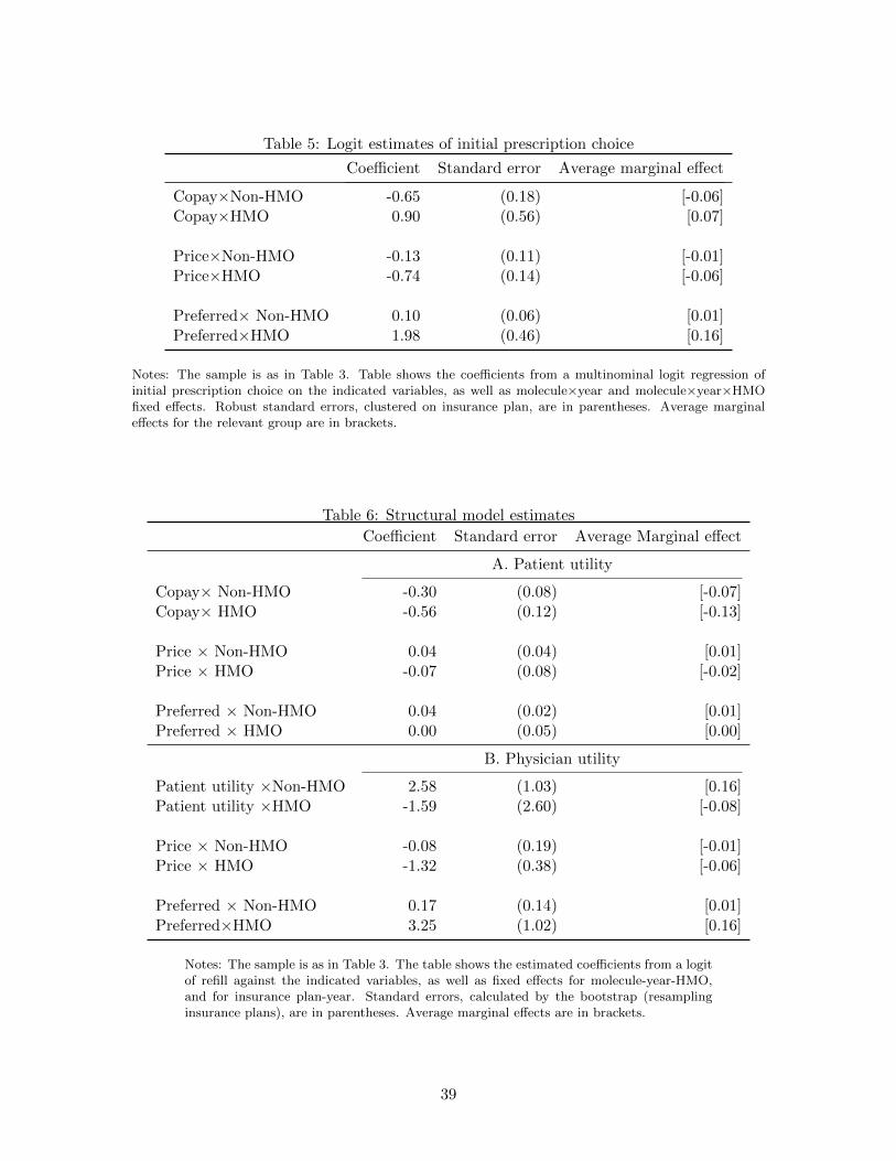
Table 5: Logit estimates of initial prescription choice

Coefficient Standard error Average marginal effect

Copay×Non-HMO -0.65 (0.18) [-0.06]Copay×HMO 0.90 (0.56) [0.07]

Price×Non-HMO -0.13 (0.11) [-0.01]Price×HMO -0.74 (0.14) [-0.06]

Preferred× Non-HMO 0.10 (0.06) [0.01]Preferred×HMO 1.98 (0.46) [0.16]

Notes: The sample is as in Table 3. Table shows the coefficients from a multinominal logit regression ofinitial prescription choice on the indicated variables, as well as molecule×year and molecule×year×HMOfixed effects. Robust standard errors, clustered on insurance plan, are in parentheses. Average marginaleffects for the relevant group are in brackets.

Table 6: Structural model estimates

Coefficient Standard error Average Marginal effect

A. Patient utility

Copay× Non-HMO -0.30 (0.08) [-0.07]Copay× HMO -0.56 (0.12) [-0.13]

Price × Non-HMO 0.04 (0.04) [0.01]Price × HMO -0.07 (0.08) [-0.02]

Preferred × Non-HMO 0.04 (0.02) [0.01]Preferred × HMO 0.00 (0.05) [0.00]

B. Physician utility

Patient utility ×Non-HMO 2.58 (1.03) [0.16]Patient utility ×HMO -1.59 (2.60) [-0.08]

Price × Non-HMO -0.08 (0.19) [-0.01]Price × HMO -1.32 (0.38) [-0.06]

Preferred × Non-HMO 0.17 (0.14) [0.01]Preferred×HMO 3.25 (1.02) [0.16]

Notes: The sample is as in Table 3. The table shows the estimated coefficients from a logitof refill against the indicated variables, as well as fixed effects for molecule-year-HMO,and for insurance plan-year. Standard errors, calculated by the bootstrap (resamplinginsurance plans), are in parentheses. Average marginal effects are in brackets.

39

Table 7: Consequences of HMO prices and price sensitivities

Scenario: Baseline Give non-HMOs...

Samesensitivityas HMOs

Sameprices

as HMOs

Same prices& sensitivity

as HMOs(1) (2) (3) (4)

Average Change relative to Baseline

A. Average within-year HMO spending differential

Assuming no rebate on preferred drugs ($) -96.15 20.34 9.86 23.49Assuming 15% rebate on preferred drugs ($) -106.06 25.04 27.20 43.96Assuming 30% rebate on preferred drugs ($) -115.98 29.74 44.54 64.43

B. Characteristics of prescribed drugs in non-HMO plans

Price ($ per day supply) 1.68 -0.08 -0.12 -0.17Copay ($ per day supply) 0.47 -0.01 0.11 0.10Pr(preferred) 0.24 0.09 0.23 0.30

C. Outcomes in non-HMO plans

Consumer surplus ($) 1211.09 -0.27 -24.04 -23.55Pr(refill) 0.63 0.00 -0.01 -0.01LDL prescribed (mg / dL) 38.57 0.50 -0.11 0.44

Notes: Table shows the effect of enrolling non-HMO patients in HMOs, under increasingly broad scenarios aboutwhat this change entails. The first column of the table shows the predicted values of the indicated statistics usingthe baseline model, i.e. the coefficients reported in Table 6, for patients in non-HMOS at baseline. The remainingcolumns show the change from the baseline implied by the model and the indicated scenario. Column (2), “samesensitivity,” gives all physicians the sensitivity to price and preferredness of HMO physicians. Column (3), “sameprices,” sets prices (insurer price, copay, and preferredness) in all plans equal to the average HMO prices in eachyear. Column (4) changes both sensitivity and prices.

40

Figure 1: Initial prescription probabilities, by year and molecule

Non-HMO

HMO

0.2

.4.6

.81997 2002 2007

A. Lipitor

Non-HMO

HMO

0.2

.4.6

.8

1997 2002 2007

B. Zocor

Non-HMO

HMO

0.2

.4.6

.8

1997 2002 2007

C. Mevacor

Non-HMO

HMO

0.2

.4.6

.8

1997 2002 2007

D. Pravachol

Pro

babi

lity

Year

Notes: Figure shows the initial prescription probability by HMO status in the Marketscan data, for the indicateddrugs, which are the four most commonly prescribed statins. Not shown are the other four drugs in the sample(Crestor, Lescol, Vytorin, and Advicor). The vertical lines indicate the first full year of generic entry for Mevacor(2002) and Zocor and Pravachol (2007).

Figure 2: Price and copay sensitivities in HMOs and other plans

Non-HMO

HMO

-.05

-.02

50

.025

.05

-.75 -.5 -.25 0 .25 .5 .75Residualized plan price

A. Residualized Pr(prescribe)

Non-HMO

HMO

-.04

-.03

-.02

-.01

0.0

1.0

2.0

3

-.2 -.1 0 .1 .2 .3Residualized copay

B. Residualized Pr(refill)

Notes: Panel A shows the probability of prescribing a given drug, plotted against its price to the insurer, separatelyfor patients in HMOs and non-HMO patients. Panel B shows the probability of refilling a given drug, plotted againstits copay, separately for patients in HMOs and non-HMOs. Both the probability and price are residualized net ofdrug-year and plan-year fixed effects. In each point, I plot average probability against average price, within eachdecile of residualized price.

41

For Online Publication

A Additional model details

A.1 Proof of results

Here I prove the assertion in Section 4.1 that healthier patients have lower demand and a greaterprice sensitivity. Given a patient in health λ and with income Y and a price of quality p, a perfectlyaltruistic physician chooses quality q to maximize patient utility net of the total cost of treatment:

q∗ = argmaxqY − pq +H(λ+ q).

The first order condition for quality q∗ is

0 = −p+H ′(q∗ + λ).

I assume that there exists an interior solution to this equation for all p and λ, denoted by q∗ =q(p, λ). By the implicit function theorem, the partial derivatives of q∗ are

∂q∗

∂λ= −1

∂q∗

∂p=

1

H ′′(λ+ q)

The first line establishes the result that demand is decreasing in health. The second line gives anexpression for price sensitivity, which is negative as H ′′ < 0. The effect of health on price sensitivityis

∂

∂λ

∂q∗

∂p= − H ′′′(q∗ + λ)

(H ′′(q∗ + λ))2 ,

As long as H ′′′ > 0, this expression is negative, meaning the absolute value of price sensitivity isgrowing in λ.

A.2 Details on calculations of equilibrium quantities

This appendix provides expressions for equilibrium spending, refill rates, consumer surplus, andthe strength of prescribed and consumed drugs.

Spending, welfare, and health Expected spending in equilibrium for patient i is obtainedby integrating expected spending over all possible drugs:

spendi(price, copay, β, w) =∑d

[30priceid × Pr(d|i, price, copay, β, w)

× (1 + 11Pr(r|d, i, price, copay))].

Price is multiplied by 30 to convert from price per day to price per fill, and the refill rate is multipliedby 11 to convert to expected spending in the first year.

Expected consumer surplus for a patient prescribed drug d is given by the patient’s utility fromfilling the initial prescription, plus the option value of having the prescription available for the next

42

11 months:

CS(d, i, copay, price) =1

−αi/30

(uPid + 11 log(1 + exp(uPid))

)where αi = αHHMO+αN (1−HMO) is patient i’s copay sensitivity. Expected consumer surplus,unconditional on the initial prescription, is therefore

CS(i, copay, price, β, w) =∑d

Pr(d|i, copay, price, β, w)CS(d, i, copay, price).

As a complement to consumer surplus, which relies on patients fully internalizing the healthbenefits of drug consumption, I also calculate the expected refill rate and the strength of prescribeddrugs and filled prescriptions. The expected refill rate for patient i is

Pr(r|i, copay, price) =∑d

Pr(r|i, d, copay, price)Pr(d|i, copay, price).

The average cholesterol reduction of consumed drugs as

∆C =∑d

∆CdPr(d|i, d, copay, price) (1 + 11Pr(d|i, copay, price)) ,

where ∆Cd is the effectiveness of drug d in reducing LDL cholesterol (reported in Table 1). Because∆C is the product of the strength of the prescribed drug and the expected number of fills, Ireport both the consumed strength (i.e. ∆C), as well as the strength of the prescribed drug itself(∑

d ∆CdPr(d|i, copay, price)).Spending differential in HMOAverage spending in HMOs, spendH,y, and non-HMOs, spendN,y in a given year is

spendH,y =1

NH,y

∑p∈Hy

∑i∈p

spendi(copayp, pricep, βMDH , wP )

spendN,y =1

NN,y

∑p∈Ny

∑i∈p

spendi(copayp, pricep, βMDN , wN ),

where NH,y and NN,y are the number of people in HMOs and not in year y, p indexes insuranceplans, and Hy and Ny are the set of HMOs and non-HMO plans in y.

B How important is joint estimation?

I use a two-step procedure to estimate the model. To investigate possible efficiency losses of thetwo-step procedure, relative to joint maximum likelihood, I conducted a small Monte Carlo study.The study focuses on 2004 data, because I found it computationally infeasible to estimate the fullmodel.27 The Monte Carlo works as follows. For each of 200 bootstrap iterations, I draw a sampleof insurance plans (with replacement). For each person in a sampled plan, I draw a set of errorsfor drug choice and for utility, and then I simulate initial prescriptions and refills. For the utilityfunctions, I use the main estimated parameters as reported in Table 6. I then estimate the model

27The main challenge is the full set of plan-year fixed effects in the patients’ utility function, which greatly complicatecalculating the gradient and Hessian of the likelihood. Focusing on a single year dramatically reduces the number ofsuch fixed effects.

43

on the simulated data, using both the two step procedure and joint estimation (i.e. by maximizingthe likelihood in Equation 5).

Appendix Table D.9 summarizes the results of the Monte Carlo simulation. The first threecolumns show the average estimate, root mean squared error, and coverage rate for the 95% con-fidence intervals for the two-step estimator. The next three columns show the analogous statisticsfor the joint estimator. There is essentially no bias in the two-step estimator, and only very slightlyhigher root mean squared error. The difference in root mean squared error is generally less than 1percent of the parameter value. Therefore there is very little efficiency gain from joint estimation,relative to two-step estimation. Indeed, the average maximized likelihoods are nearly the same forthe two estimators, meaning that there is very little loss of information with two-step estimation.The table does show one important difference between the estimators, however: the coverage ratefor the 95% confidence intervals from two-step estimation are well below their nominal values,especially for the HMO physician preferences.28 To achieve proper coverage, I therefore use thebootstrap to calculate confidence intervals.

C Testing for unobserved match quality

C.1 Testable implication of match quality

Here I present a simple model in which physicians match patients to drugs on the basis of apatient-specific match quality term. The point is to develop a clear, testable implication of thehypothesis that physicians match patients to drugs on the basis of unobserved match quality. Thekey implication is that if match quality is important, then the observed refill rate of one drugdepends on the copay of the other drugs. The intuition for this is that as the copay of one drug(say, Lipitor) rises, more patients receive a prescription for another drug (say, Zocor). If matchquality is important, then the first patient to receive a prescription for Zocor should be the bestmatch; the marginal patient prescribed Zocor has a lower match quality than the average patient.Thus the increase in Lipitor’s copay brings down the average match quality of people prescribedZocor, reducing average refill rates.

To show this result as clearly as possible, the matching model in this section abstracts frommany of the rich details of the empirical model. In particular, in this model physicians are assumedto prescribe the drug which maximizes their patients’ utility, and that the only drug characteristicis its copay.

Patient i derives utility uid from drug d, with

uid = αd − βcopayid + γid, (C.6)

where αd is average quality of drug d, copayid is the copay of the drug, and γid an idiosyncraticmatch quality. I assume that γ ∼ F , with mean zero. For the moment I make no further restrictionon F .

The patient refills a prescription for drug d if its utility exceeds an idiosyncratic refill cost,distributed IID according to some distribution R. Let Rd(copayid, γid) ≡ R(αd − βcopayid + γid)be the probability that a patient i refills drug d if her match quality is γid and her copay for d iscopayid.

To keep the model tractable, I assume that the physician prescribes the drug with the highest

28These confidence intervals are the cluster robust confidence intervals for maximum likelihood.

44

utility to the patient (gross of the refill cost). Letting d∗i indicate the prescribed drug, we have

d∗i = argmaxd∈{1,2}uid (C.7)

The physician prescribes drug 1 if ui2 ≥ ui1, or equivalently if

δ ≡ γ2 − γ1 ≤ (α1 − α2)− β(copay1 − copay2) ≡ ∆(copay). (C.8)

δ is the difference between the match quality for the two drugs, and ∆(copay) is the difference inthe observable part of utility; this is a function of the vector of copays. Let Fδ be the marginaldistribution of δ (determined by F ). The probability drug 1 is prescribed is Fδ(∆(copay)).

In the data, we only observe refills of the prescribed drug. The probability of refill for drug 1,conditional on a prescription for drug 1, is

Pr(refill|d∗ = 1, copay) =1

Fδ(∆(copay))

∫ δ=∆(copay)

δ=−∞

∫γ1

R1(copay1, γ1)fγ1|δ(γ1)dγ1fδ(δ)dδ (C.9)

The inner integral is the average refill rate, averaging over the conditional distribution of γ1 givenδ. The outer integral integrates over the distribution of δ, but the range of integration accounts forthe fact that at some values of δ, drug 1 is not prescribed.

Proposition C.1. Suppose γ ∼ N(0,Σ), with

Σ =

[σ2

1 σ12

σ22

]and σ12 < σ2

1 Then∂Pr(refill|d∗ = 1, copay)

∂copay2< 0 (C.10)

Before proving Proposition C.1, I provide a few comments. The general intuition is that themarginal person to get drug 1—who is just indifferent between drug 1 and drug 2— has a lowerutility for drug 1 than the average person, so when the copay of drug 2 goes up, the average refill rateof everyone prescribed drug 1 falls. This intuition does not hold, however, for every possible jointdistribution of γ1 and γ2, and hence some restrictions are needed. A sufficient conditions is that γ1

and γ2 are jointly normal and not too correlated (i.e. σ12 < σ21). The conditions in Proposition C.1

generalize those used in the empirical literature on physician prescribing decisions with unobserveddrug quality, which assumes that match quality is normally distribution and independent acrossdrugs (e.g. Coscelli and Shum 2004, Crawford and Shum 2005, Ching 2010a, Ching 2010b, Liu,Liu and Chingtagunta 2017).

To understand the requirement that σ12 < σ21, consider the extreme case where γ1 and γ2 are

highly correlated, but the variance of γ2 is much larger than the variance of γ1. In that case, thefirst person prescribed drug 1 has a very negative of γ2, not necessarily a high value of γ1. Themarginal person prescribed drug 1 has a high value of both γ2 and γ1; possibly higher than theaverage value of γ1.

To prove the result, let g(δ, copay1) =∫R(copay1, γ1)fγ1|δ(γ1)dγ1. This is the average refill

rate of drug 1 when the difference in match qualities is δ. Note that g(δ, copay1) > g(δ′, copay1)whenever Fγ1|δ first order stochastically dominates Fγ1|δ′ , because R is an increasing function of γ1.

45

A bit of algebra and the fundamental theorem of calculus show that

∂

∂copay2Pr(refill|d = 1, copay) = β

fδ(∆(copay))

Fδ(∆(copay))

[g(∆(copay))−

∫δ≤∆p

g(δ)fδ(δ)dδ

F (∆(copay))

](C.11)

The term outside of brackets is positive, so the derivative is negative as long as the first term inbrackets is smaller than the second term in brackets. The first term is the marginal refill rate: therefill rate of people who are just on the margin of being prescribed drug 1. The second term isthe average refill rate, averaging over everyone prescribed drug 1. The entire expression is negativeas long as the average refill rate is larger than the marginal refill rate. A sufficient condition istherefore that g(δ) is decreasing in δ. To show this condition, it suffices to show that Fγ1|δ=d firstorder stochastically dominates Fγ1|δ=d′ whenever d < d′.

Wwe can derive an exact expression for fγ|δ because γ and δ are jointly normal:

γ1|δ = d ∼ N

(σ12 − σ2

1

σ21 + σ2

2 − 2σ12d, σ2

1 −(σ12 − σ2

1

)2σ2

1 + σ22 − 2σ12

),

so

Fγ1|δ=d(γ) = Φ

γ − σ12−σ21

σ21+σ2

2−2σ12d

σ21 −

(σ12−σ21)

2

σ21+σ2

2−2σ12

This expression is decreasing in d whenever σ12 − σ2

1 < 0. Thus if d > d′, Fγ1|δ=d′(γ) < Fγ1|δ=d(γ)for all γ, which completes the proof.

C.2 Empirical tests of match quality

The model in the previous section suggests a straightforward test for match quality: look atwhether the refill rate of drug d depends on the copay of drug d′. To implement this test, for eachdrug d available to patient i in year t, I define the copay

idtand p

idtto be the lowest copay and

lowest price among drugs d′ 6= d available to i in t. I then estimate the following logistic regression:

Pr(refillidt) = L(η1copayidt + η2priceidt + αPNcopayid × (1−HMOi) + αPHcopayid ×HMOi

+ βPNpriceid × (1−HMOi) + βPHpriceid ×HMOi

+ γPNprefid × (1−HMOi) + γPHprefid ×HMOi

+µPdy + µPdyH ×HMOi + θPp(i)

)(C.12)

This is the same specification used to estimate patient utility, except augmented to include copayand p. I include these variables not to control for patient-drug matching, but rather as a test ofthe null hypothesis of no such matching. Under the null hypothesis we expect η1 to be zero; underthe alternative hypothesis we expect it to be negative.

Appendix Table D.8 shows the results. In column (1) I present the baseline results. In column(2) I control for interactions between copay and HMO, and in column (3) I control for priceinteracted with HMO. The coefficients on copay are positive, small and insignificant. Tests forjoint significance of the alternative-copay coefficients fail to reject that they are jointly equal to

46

zero in column 2 (p = 0.20) or in column 3 (p = 0.23 for the hypothesis that the alternative copaycoefficients are zero, and p = 0.47 for the hypothesis that the alternative copay and price coefficientsare jointly zero). Therefore the refill data are consistent with the hypothesis that physicians do notmatch patients to drugs on the basis of unobserved match quality. Although it is difficult to assessthe power of this test, it is reassuring that the coefficients are positive, as this is the wrong-signedfrom the perspective of the patient-drug matching hypothesis.

It might be surprising that the data are consistent with no patient-drug matching, as a largeliterature (going back at least to Crawford and Shum (2005)) has found evidence for heterogeneousmatch quality in prescription drugs. These results are consistent with that literature. The resultshere suggest that at the time of writing the initial prescription, physicians have little informationavailable to them (beyond what the econometrician observes) that is useful for forecasting refillrates. The literature on match quality finds that it can take multiple prescriptions for physiciansto find the right match for their patients—a finding consistent with the possibility that physicianshave relatively little private information at the time of writing the initial prescription.

D Sensitivity analysis

This appendix provides extensive sensitivity analysis, showing that the results are not sensitiveto weaker identifying assumptions, alternative modelling choices, and alternative ways of definingprices. Table D.6 shows the results, with the base results in column (1) Panel A shows the pointestimates for patients, Panel B for physicians, and Panel C the main counterfactual results (obtainedfrom giving non-HMO physicians the price sensitivity of HMO physicians). In column (2), I addrich controls for patient health to both the patient and the physician utility function. These area set of interactions between drug fixed effects and dummies for each of seven aspects of patienthealth: whether patients have a past diagnosis for a cholesterol disorder, diabetes, heart disease, orhypertension; whether their age and sex put them at risk for heart disease; and dummy variablesfor Charlson comorbidity index of one or at least two. These controls let patient drug preferencesvary with their health status in a flexible way, so that sicker patients (or their physicians) may havea taste for stronger drugs, for example. Including these additional controls has no meaningful effecton any of the point estimates, and only a small effect on the counterfactuals; the change in spendingis now about $2 smaller in absolute value. This columns shows that the controlling for observabledifferences in patient health does not affect the point estimates. This suggests that physicians arenot effectively matching patients to drugs even on the basis of easily observed conditions, such aspast heart disease, age, or sex. It is perhaps unlikely, then, that they are matching on the basis ofunobserved heterogeneity, subtler characteristics not observed in the claims data.

One concern about the results is that I let patient utility depend on prices (not just copay).Although I find a small and insignificant price effect for patients, this effect absorbs some HMOprice sensitivity. In column (3), I drop price from the patient utility function. A final threatto identification is that patients may select insurance plans that have good coverage for theirparticular drug needs,. To address this concern, I attempt to isolate price variation that only comesacross companies, rather than across insurance plans within an employer. For such variation to becorrelated with patient preferences, patients would have to seek out a job with insurance that hasparticularly good coverage of a particular drug, given the plan’s overall quality (which the insuranceplan-year fixed effects control for). To isolate cross-employer price variation, I use a control functionapproach, which works as follows. Pooling all insurance plan-years and drugs, I regress copaysand prices on employer-year-drug fixed effects. (To be precise, I regress copay×HMO, copay×(1-HMO), price×HMO, and price×(1-HMO) on contributor-drug-year fixed effects. A contributor is

47

an organization providing data to Marketscan, which I assume is an employer providing healthinsurance.) These fixed effects are the average prices of each drug for a given employer-year.The residuals from this regression represent plan-specific deviations within an employer. I controlfor these residuals in the patients’ and in the physicians’ utility functions (interacted with HMOstatus), so that the only remaining price variation is across employer, rather than across plan, withinemployer. This is comparable to using employer-drug average copays and prices as instrumentsfor plan-drug specific copays and averages. The results from this procedure are in column (4).The estimated copay sensitivity falls by about a quarter for patients in HMOs, consistent withsome matching. But the estimated physician utility function is largely unchanged, and so thecounterfactuals are also highly similar.

In the columns (5) and (6) I investigate the sensitivity of the results to the discount factor.I consider two extreme choices: δ = 0 in column (5) and δ → 1 in column (6). When δ = 0,the physician does not account for future non-refilling, and her value function becomes her drug-specific utility, uMD. When δ → 1, the physician places all weight on future periods, and so hervalue function is Pr(r|d)uMD. The choice of δ does not affect patient preferences. It mechanicallychanges the scale of physician utility, but results in similar marginal effects for the prescribingdecision, as well as similar counterfactuals.

Finally in columns (7) and (8) I show sensitivity to alternative ways of handling prices andpreferredness. In column (7), I drop the 11 plan years that have imputed drug prices, i.e. drug-plan-year cells with zero days’ supply purchased. This does not materially affect the results. Incolumn (8), I define tiers as $2 wide instead of $5 wide. This changes slightly the set of preferreddrugs. The results are highly similar, however. Overall, therefore, the results appear robust toweaker identification assumptions, to alternative choices of δ, and to alternative ways of handlingprices.

48

Table D.1: Prevalence of managed care features

Plan type Fully capitated HMOs Other MCOs Non-MCOs(1) (2) (3)

Fraction with utilization review 0.36 0.27 0.19(0.06) (0.02) (0.07)

Difference, relative to HMOs -0.10 -0.17(0.09) (0.09)

Fraction with case management 0.39 0.47 0.60(0.06) (0.03) (0.09)

Difference, relative to HMOs 0.08 0.22(0.11) (0.11)

Fraction with precertification requirements 0.62 0.73 0.75(0.05) (0.02) (0.07)

Difference, relative to HMOs 0.11 0.12(0.09) (0.09)

# Plan-years 88 427 63

Notes: Table shows the fraction of plans of the indicated type that have utilization review, case management, andprecertification requirements, as well as the difference relative to HMOs for non-HMO managed care organizationsand non-managed care organization plans. Robust standard errors, clustered on plan, in parentheses.

Table D.2: Plan-tiers account for most copay variation

Plans All Has formulary 2 tiers 3 tiers 4 tiers(1) (2) (3) (4) (5)

µcopay 0.528 0.698 0.680 0.826 0.831σcopay 0.386 0.409 0.406 0.408 0.462σcopay| plan-year FE 0.253 0.341 0.339 0.349 0.461σcopay| plan-year-tier FE 0.077 0.096 0.097 0.087 0.019

# Plans 578 308 262 41 5

Notes: Table shows reports the average out-of-pocket price of prescriptions (per days supply), its standard deviation,and its standard deviation net of plan-year fixed effects and net of plan-year-tier fixed effects, for different groups ofplans: all plans in column (1), plans with formularies (as defined in Section 3) in column 2, and plans with formularieswith 2, 3, or 4 tiers. The standard deviations net of plan-year or plan-year-tier fixed effects are obtained as rootmean squared errors from regressions of out-of-pocket price on plan-year or plan-year-tier fixed effects, weighted byplan size.

49

Table D.3: Logit estimates of initial prescription choice, plan-type specific coefficients

Coefficient Standard error Marginal effect

Copay×HMO 0.903 (0.562) [0.074]Price×HMO -0.735 (0.140) [-0.061]Preferred× HMO 1.981 (0.461) [0.163]

Copay× Basic/comprehensive -1.358 (0.398) [-0.138]Copay× EPO -1.557 (0.555) [-0.150]Copay× Non-capitated POS -0.484 (0.160) [-0.046]Copay× PPO -0.609 (0.180) [-0.058]Copay× Capitated POS -0.487 (0.143) [-0.055]Copay× CDHP -0.570 (0.169) [-0.053]

Price× Basic/comprehensive -0.317 (0.111) [-0.032]Price× EPO 0.088 (0.345) [0.008]Price× Non-capitated POS -0.046 (0.110) [-0.004]Price× PPO -0.132 (0.105) [-0.013]Price× Capitated POS 0.126 (0.136) [0.014]Price× CDHP 0.113 (0.165) [0.010]

Preferred× Basic/comprehensive 0.015 (0.107) [0.002]Preferred× EPO 0.115 (0.135) [0.011]Preferred× Non-capitated POS 0.191 (0.072) [0.018]Preferred× PPO 0.066 (0.068) [0.006]Preferred× Capitated POS 0.143 (0.128) [0.016]Preferred× CDHP -0.101 (0.119) [-0.009]

Notes: The sample is as in Table 3. Table shows the coefficients from a multinominal logit regression ofinitial prescription choice on the indicated variables, as well as molecule×year and molecule×year×HMOfixed effects. Robust standard errors, clustered on insurance plan, are in parentheses. Average marginaleffects for the relevant group are in brackets.

50

Table D.4: Logit estimates of initial prescription choice, accounting for managed care features

Coefficient Standard error Marginal effect

Copay × HMO 0.922 (0.570) [0.076]Price × HMO -0.727 (0.144) [-0.060]Preferred× HMO 1.947 (0.471) [0.160]

Copay × Non-HMO -0.649 (0.249) [-0.064]Price × Non-HMO -0.125 (0.120) [-0.012]Preferred × Non-HMO 0.093 (0.068) [0.009]

Copay× Case management -0.123 (0.140) [-0.012]Copay × Utilization review -0.094 (0.205) [-0.009]Copay × Precertification -0.056 (0.053) [-0.006]

Price × Case management -0.056 (0.053) [-0.006]Price × Utilization review 0.051 (0.065) [0.005]Price × Precertification 0.082 (0.101) [0.008]

Preferred × Case management 0.148 (0.078) [0.015]Preferred × Utilization review 0.049 (0.076) [0.005]Preferred × Precertification -0.105 (0.085) [-0.010]

Notes: The sample is as in Table 3. Table shows the coefficients from a multinominal logit regression of initialprescription choice on the indicated variables, as well as molecule×year and molecule×year×HMO fixedeffects. Robust standard errors, clustered on insurance plan, are in parentheses. Average marginal effectsfor the relevant group are in brackets. Average marginal effects for the interactions should be interpreted asdifferential marginal effects.

51

Table D.5: Decomposition of drug-year fixed effects in patient utility

Patient utility Differential HMO patient utility(1) (2)

LDL reduction 0.010 -0.001(0.004) (0.010)

Generic drug 0.074 -0.157(0.094) (0.245)

Combination drug 0.020 0.073(0.081) (0.199)

Molecule age 0.006 0.004(0.009) (0.019)

Year fixed effects? Yes YesMolecule-years 63 63R2 0.35 0.42

Notes: The table shows the estimated coefficients from a regression in which the dependent variable is the estimateddrug-year fixed effect in the patient’s utility function (column (1)) or the estimated differential drug-year fixed effectin HMO patient’s utility (column (2)). The controls are as indicated. LDL reduction is the molecule’s effectivenessin reducing LDL cholesterol; generic drug is an indicator for whether the drug is off-patent, combination drug is anindicator for combination products, and molecule age measures the number of years since the molecule entered themarket. Robust standard errors in parentheses.

52

Table D.6: Sensitivity analysis

BaseHealth

ControlsNo price

in uPNo planselection

δ = 0 δ → 1No

imputationFormulary Tiers

$2 wide(1) (2) (3) (4) (5) (6) (7) (8)

A. Patient utility function

Copay x Non-HMO -0.30 -0.30 -0.33 -0.30 -0.30 -0.30 -0.31 -0.28(0.08) (0.08) (0.06) (0.08) (0.08) (0.08) (0.08) (0.08)

Copay x HMO -0.56 -0.58 -0.50 -0.50 -0.56 -0.56 -0.57 -0.58(0.12) (0.11) (0.09) (0.15) (0.13) (0.13) (0.13) (0.14)

Price x Non-HMO 0.04 0.04 - 0.05 0.04 0.04 0.04 0.04(0.04) (0.04) - (0.04) (0.04) (0.04) (0.04) (0.04)

Price x HMO -0.07 -0.08 - -0.11 -0.07 -0.07 -0.08 -0.07(0.08) (0.08) - (0.09) (0.08) (0.08) (0.09) (0.08)

Preferred x Non-HMO 0.04 0.05 0.04 0.02 0.04 0.04 0.05 0.06(0.02) (0.02) (0.02) (0.03) (0.02) (0.02) (0.02) (0.02)

Preferred x HMO 0.00 0.00 -0.00 0.07 0.00 0.00 -0.00 -0.01(0.05) (0.05) (0.05) (0.07) (0.05) (0.05) (0.05) (0.05)

B. Physician utility function

Patient utility x Non-HMO 2.58 1.21 2.46 2.26 2.18 2.55 2.37 2.57(1.03) (0.74) (0.95) (1.02) (0.63) (1.08) (0.98) (1.03)

Pat utility x HMO -1.59 -0.76 -1.86 -0.76 -1.61 -1.58 -2.42 -1.74(2.60) (0.69) (2.77) (2.36) (1.74) (2.34) (2.94) (2.59)

Price x Non-HMO -0.08 0.10 0.01 -0.18 -0.21 -0.07 -0.09 -0.07(0.19) (0.10) (0.16) (0.21) (0.13) (0.20) (0.19) (0.18)

Price x HMO -1.32 -1.32 -1.16 -1.55 -0.85 -1.33 -1.30 -1.27(0.38) (0.23) (0.35) (0.37) (0.24) (0.35) (0.42) (0.34)

Preferred x Non-HMO 0.17 0.33 0.15 0.15 0.01 0.17 0.19 0.14(0.14) (0.10) (0.13) (0.13) (0.08) (0.14) (0.13) (0.13)

Preferred x HMO 3.25 3.08 3.21 3.50 1.99 3.27 3.38 3.09(1.02) (0.35) (0.97) (1.00) (0.72) (1.00) (1.16) (1.04)

C. Counterfactual Effect of HMO price sensitivity

Spending differential, no rebate 20.25 26.14 18.33 22.38 13.35 20.48 19.22 20.21Spending differential, 15% rebate 24.95 30.01 23.12 27.29 18.75 25.16 24.20 24.22Spending differential, 30% rebate 29.65 33.88 27.92 32.20 24.14 29.83 29.19 28.24Price ($ per day supply) -0.08 -0.10 -0.07 -0.09 -0.05 -0.08 -0.07 -0.08Copay ($ per day supply) -0.01 -0.01 -0.01 -0.01 -0.01 -0.01 -0.01 -0.01Pr(Preferred) 0.09 0.07 0.09 0.09 0.10 0.09 0.09 0.08Consumer surplus ($) -0.28 -0.51 0.38 -0.87 1.91 -0.35 -0.16 -1.65Pr(refill) 0.00 0.00 0.00 0.00 0.00 0.00 0.00 0.00LDL prescribed (mg / dL) 0.50 -0.42 0.50 0.52 0.56 0.49 0.52 0.48

Notes: Sample is as defined in Table 3. The patient utility function is estimated from a logit of refill againstthe indicated controls, as well molecule-year-HMO and insurance plan-year fixed effects. “Health controls”adds patient diagnoses interacted with molecule fixed effects (see Appendix A for details). “No price in patu” excludes drug price from the patient’s utility function. “No plan selection” adds the residuals from aregression of drug prices on drug-year-employer fixed effects. “No imputation” drops people in insuranceplans with any imputed prices. “Formulary tiers $2 wide” defines formulary tiers to be $2 wide ratherthan $5 wide. For the physician utility function estimation, see text. For readability, physician preferenceparameters are scaled by 100 (except in columns 5). The counterfactuals show the effect of giving non-HMO physicians physicians the price sensitivity of HMO physicians. Standard, reported in parentheses, arecalculated by the bootstrap, resampling insurance plans.

53

Table D.7: Diagnosis-specific coefficients from health controls specification

HighCholesterol

DiabetesHeart

DiseaseHypertension

AgeRisk

Female1 Charlson

Comorbidity≥ 2 CharlsonComorbidities

(1) (2) (3) (4) (5) (6) (7) (8)

Main 0.22 0.01 0.10 0.10 0.39 -0.03 0.00 0.13(0.01) (0.01) (0.01) (0.01) (0.01) (0.01) (0.01) (0.02)

× Zocor -0.00 -0.02 -0.01 -0.02 -0.01 0.02 0.01 -0.05(0.01) (0.01) (0.02) (0.01) (0.01) (0.01) (0.01) (0.03)

× Mevacor -0.12 0.09 -0.15 0.03 0.02 0.10 -0.05 -0.07(0.04) (0.03) (0.04) (0.02) (0.02) (0.02) (0.03) (0.06)

× Pravachol 0.04 0.03 -0.04 -0.02 -0.04 -0.01 -0.03 0.05(0.02) (0.03) (0.02) (0.02) (0.02) (0.02) (0.02) (0.04)

× Crestor -0.06 0.00 -0.08 -0.00 -0.04 0.01 0.00 0.07(0.02) (0.02) (0.02) (0.02) (0.02) (0.02) (0.02) (0.05)

× Lescol 0.00 0.03 -0.04 -0.00 -0.02 -0.00 0.03 -0.06(0.04) (0.04) (0.04) (0.04) (0.03) (0.03) (0.04) (0.07)

× Zetia -0.05 0.00 -0.05 -0.01 0.01 0.04 -0.05 0.00(0.03) (0.02) (0.02) (0.02) (0.02) (0.02) (0.03) (0.05)

× Advicor -0.04 0.02 0.03 -0.01 0.08 -0.11 0.04 -0.03(0.05) (0.05) (0.04) (0.05) (0.05) (0.05) (0.07) (0.13)

P-value ofjoint test 0.00 0.00 0.00 0.00 0.00 0.00 0.26 0.00

Notes: Table reports the main effect for health conditions, and the coefficient on the interaction between healthconditions and drug dummies, in patient utility functions, which are estimated in Column (2) of Appendix TableD.6. Each column corresponds to a different main effect, reported in the first row. The subsequent rows show theinteraction between that health condition and dummy variables for the indicated molecule. Standard errors arecalculated by the bootstrap, resampling plans. P-values of the test of joint significance for each group of interactionsare based on cluster-robust variance-covariance matrix.

54

Table D.8: Testing for patient-drug matching

Base Control for cheapest Control for cheapestSpecification alternative copay alternative copay

& alternative price(1) (2) (3)

Copay × Non-HMO -0.30 -0.28 -0.28(0.07) (0.08) (0.08)

Price × Non-HMO 0.04 0.04 0.03(0.04) (0.04) (0.04)

Copay × HMO -0.56 -0.56 -0.57(0.09) (0.09) (0.11)

Price × HMO -0.07 -0.07 -0.08(0.06) (0.06) (0.06)

Preferred × Non-HMO 0.04 0.05 0.05(0.02) (0.02) (0.02)

Preferred × HMO 0.00 0.00 -0.00(0.04) (0.04) (0.05)

Cheapest alternative copay × Non-HMO 0.16 0.15(0.09) (0.09)

Cheapest alternative copay × HMO 0.04 0.05(0.20) (0.21)

Cheapest alternative price × Non-HMO -0.02(0.07)

Cheapest alternative price × HMO 0.02(0.09)

Notes: The sample is as in Table 3. Table shows the coefficients from a logit regression of refill against theindicated characteristics of the prescribed drug, as well as drug-year-HMO fixed effects and insurance plan-year fixed effects. Under the hypothesis of patient-drug matching, own refill rates should be increasing in theprices of alternative drugs. Column (2) therefore adds controls for the lowest copay among non-prescribeddrugs, interacted with HMO, and column (3) adds controls for the lowest price among non-prescribed drugs.Robust standard errors, clustered on plan, in parentheses.

55

Table D.9: Joint estimation produces very small efficiency gains

Two-step estimation Joint estimationAvg. estimate RMSE Coverage Avg. estimate RMSE Coverage

A. Patient parameters

Copay × Non-HMO -0.298 0.0041 0.910 -0.297 0.0040 0.975Price × Non-HMO 0.037 0.0029 0.940 0.037 0.0028 0.960Preferred × Non-HMO 0.043 0.0034 0.925 0.043 0.0033 0.960Copay× HMO -0.562 0.0127 0.920 -0.561 0.0120 0.990Price × HMO -0.075 0.0060 0.915 -0.075 0.0059 0.995Preferred × HMO 0.005 0.0102 0.925 0.005 0.0098 0.990

B. Physician parameters

uP utility × Non-HMO 2.594 0.0933 0.940 2.594 0.0928 0.800Price × Non-HMO -0.075 0.0131 0.920 -0.075 0.0131 0.990Preferred × Non-HMO 0.164 0.0238 0.895 0.164 0.0238 0.980uP × HMO -1.580 0.1546 0.870 -1.582 0.1539 0.905Price × HMO -1.321 0.0402 0.765 -1.322 0.0394 0.995Preferred × HMO 3.245 0.0642 0.805 3.245 0.0639 0.990

Average log likelihood -4452172 -4452171

Notes: Table shows the result of a Monte Carlo experiment investigating the efficiency gains from jointestimation. In each of 200 iterations, I take a random sample of insurance plans in 2004 (with replacement),and then simulate and estimate the model. The table reports the average parameter estimates, root meansquared error, and coverage rates of 95% confidence intervals (clustered on insurance plan).

56