Embed Size (px)
Citation preview
Chapter 1
Why Study Information Choice?
The developed world is increasingly becoming a knowledge-driven economy. Fewer and fewer
workers are involved in producing goods. Instead, much of value added comes from activities
like consulting, forecasting or financial analysis. Even within traditional firms, significant
resources are devoted to activities such as managerial decision making, price setting or eval-
uating potential investments, each of which involves acquiring, processing and synthesizing
information. Most macroeconomic models focus on goods production with capital and labor
as inputs and constant returns to scale. Similarly, most portfolio and asset pricing theo-
ries model the investment decisions that maximize investors’ utility. Only a small body of
research tells us about the information acquisition that regulates these production and in-
vestment decisions, even as the amount of resources devoted to information-related activities
grows ever larger.
Every expectation, mean, variance, covariance, every moment of every random variable is
conditional on some information set. Typically, we think of that information set as consisting
of all the past realizations of the variable. But, what if agents in the model do not know the
entire history of all the realizations? Or, alternatively, what if they have information in ad-
dition to the history? Which information set agents have will typically change every moment
of the random variable. The information does not aÆect what the future realizations of the
random variable will be. It changes what agents know about those realizations. Moments of
a random variable summarize what someone knows about it.
Since means, variances and covariances appear all over economics and finance, how agents
in our models evaluate these moments aÆects how they behave in any environment where a
11
12 CHAPTER 1. WHY STUDY INFORMATION CHOICE?
random variable matters. The eÆect of stochastic changes in productivity in a business cycle
model, of changes in asset valuation in a portfolio problem, of shocks to endowments in a
consumption-savings problem, of money supply shocks in a price-setting problem, or changes
in the state in a coordination game, all depend on what information people know.
This manuscript describes both a narrow and a broad research area. It focuses narrowly
on predicting what information agents have and how that information aÆects aggregate out-
comes. It presents a toolkit for writing applied theories: It does not explore theory so much
for its own sake. Rather, it explores theories that provide explanations for the phenomena
we see in the world around us. The applications are wide-ranging, from asset pricing to
monetary economics to international economics to business cycles. This book covers both
the mathematical structures necessary to work in this area and ways of thinking about the
modeling choices that arise. My hope is that at the end, the reader will be at the frontier of
applied theory research in information choice and might be inspired to contribute to it.
1.1 Types of Learning Models
The literature on learning is expansive. Before delving into the material, here is an overview
of what kinds of subjects are covered here and what is omitted.
Learning is also often used to refer to a distinct literature on non-Bayesian learning. One
example is adaptive least-squares learning, where agents behave as econometricians, trying
to discover the optimal linear forecasting rule for next period’s state. Evans and Honkapohja
(2001) oÆer an exhaustive treatment of this literature. Information frictions also feature
prominently in settings where agents do not know the true model of the economy and make
decisions that are robust to model misspecification (Hansen and Sargent (2003)). This book
focuses exclusively on environments where agents update their information sets using Bayes’
law. They know the true model of the economy and are uncertain only about which realization
of the state will be drawn by nature. Agents in this class of models are not uncertain about
the distribution of outcomes from which nature draws that state. They have (noisy) rational
expectations. This focus creates a distinction between the study of the process through which
agents learn and the information that they acquire and learn from. It allows for a deeper
understanding of what information agents observe, by making simple assumptions about how
that information is used to learn.
Among models with Bayesian learning, there are models of passive learning and models
1.1. TYPES OF LEARNING MODELS 13
of active learning. In passive learning models, agents are endowed with signals and/or learn
as an unintended consequence of observing prices and quantities. One set of examples are
models where information is exogenous. Information may be an endowment, as in Morris and
Shin (1998), or it may arrive stochastically as in Mankiw and Reis (2002). But agents can
be passive learners, even when information is endogenous. For example, information could
be produced as a by-product of other activity or information could be conveyed by market
prices. Even in these settings, agents are not exercising any control over the information
they observe.
The other way people acquire information is intentionally, by choice. Acquiring informa-
tion by choice is also called active learning. This choice might involve purchasing information,
choosing how to allocate limited attention or choosing an action, taking into account the in-
formation it will generate. Such models go beyond explaining the consequences of having
information; they also predict what information agents will choose to have. Active learning is
starting to play a more prominent role in macroeconomics and finance. In macroeconomics,
it has been used to re-examine consumption-savings problems (Sims, 1998), price-setting
frictions (Mackowiak and Wiederholt (2009b) and Reis (2006)) and business cycle dynamics
(Veldkamp and Wolfers, 2007). In finance, active learning has a long tradition in investment
allocation models (Grossman and Stiglitz (1980), Hellwig (1980)) and has more recently
been used in dynamic asset pricing theories (Peng and Xiong, 2006), models of mutual funds
(Garcia and Vanden, 2005) and models of decentralized trade (Golosov et al., 2008).
The vast majority of papers in dynamic macro and finance still employ passive learning.
Beliefs change when agents observe new outcomes or when new signals arrive, because the
model assumes they do. While such models clarify the role of information in aggregate
outcomes, they do not tell us what information we may or may not observe. Models of
active learning complement this literature by predicting what information agents choose to
observe. Because an active learning model can predict information sets on the basis of
observable features of the economic environment, pairing it with a passive learning model
where information predicts observable outcomes results in a model where observables predict
observables. That is the kind of model that is empirically testable. If the goal is to write
applied theories that explain observed phenomena, we need a testable theory to know if the
proposed explanation is correct. Therefore, while this book devotes substantial attention to
passive learning models which form the bulk of the literature, it systematically complements
this coverage with a discussion of how information choice aÆects the predictions.
14 CHAPTER 1. WHY STUDY INFORMATION CHOICE?
Bayesian learning models are also used prolifically in other literatures. While this book
focuses on applications of interest to researchers in macroeconomics and macro-finance, others
cover related topics that this book only touches on: Vives (2008) and Brunnermeier (2001)
focus on market microstructure and information aggregation in rational expectations markets;
Chamley (2004) explores models of herding where agents move sequentially and learn from
each others’ actions. Each of these volumes would be a good complement to the material
presented here.
1.2 Themes that Run Through the Book
Theme 1: Information choice bridges the gap between rational and behavioral
approaches. The first theme is about the place information-based models occupy in the
macroeconomics and finance literature. We look to incomplete information models in situ-
ations where the standard full-information, rational models fail to explain some feature of
the data. Since these are the same set of circumstances that motivate much of the work in
behavioral economics, modeling incomplete information is an alternative to the behavioral
economics approach. Both literatures take a small step away from the fully-informed, ex-
post optimal decision making that characterizes classical macroeconomics and finance. This
is useful because adding this incomplete information allows the standard models to explain a
broader set of phenomena, such as portfolio under-diversification, asset price bubbles, sticky
prices or inertia in asset allocation.
The line between incomplete information and behavioral assumptions can be further
blurred because some approaches to modeling incomplete information – for example infor-
mation processing constraints – are a form of bounded rationality. Yet, there is a fundamental
distinction between the two approaches.
At its core, information choice is a rational choice. Agents in information choice models
treat their information constraints just like agents in a standard model treat their budget
constraints. Rather than attacking tenets of the rational framework, information choice seeks
to extend it by enlarging the set of choice variables. The advantage of this approach is that
requiring information sets to be a solution to a rational choice problem disciplines the forms
of information asymmetry one can consider in a given environment.
Theme 2: Information is diÆerent from physical goods because it is non-
rival and has increasing returns to scale. Information is expensive to discover and
1.2. THEMES THAT RUN THROUGH THE BOOK 15
cheap to replicate. That property often produces corner solutions and complementarities in
information choice problems that makes the predictions of models with information choice
fundamentally diÆerent from those without it (Wilson, 1975).
The fact that the economics of producing information is so diÆerent from the economics of
producing physical goods allows information choice models to explain phenomena that pose
a challenge to standard theory. This idea shows up in the discussion of information choice
and investment, where agents value information about a larger asset more because one piece
of information can be used to evaluate every dollar of the investment. It reappears in the
section on information markets where information has a market price that decreases in the
quantity of information sold because it is free to replicate. That makes observing information
that others observe a cost-eÆective strategy.
Theme 3: Correlated information or coordination motive? A large literature
in economics and finance studies situations where many agents take similar actions at the
same time. Examples include bank runs, speculative attacks, market bubbles and fads. The
most common explanation is the existence of a coordination motive: Agents want to behave
similarly because acting like others directly increases their utility. Yet, in some settings,
agents appear to be acting as if they had a coordination motive when no such motive is
apparent. An alternative explanation is that agents observe correlated information, which
leads them to behave similarly. One example is the theory of herds, which is based on the
following parable, taken from Banerjee (1992): Suppose that a sequence of diners arrive at
two adjacent restaurants, A and B. The first and second diners believe A to be the better
restaurant. So, both dine there. The third diner believes that B is the better restaurant, but
sees no one there. He infers that the two diners in restaurant A must have had been told
that A was better and chooses A over B. All subsequent diners make similar calculations
and dine at restaurant A. Thus sequential, publicly-observable actions provide one reason
that agents could have similar information sets. An alternative reason why agents may have
similar information is based on information choice. In the language of the parable, all the
diners might go to restaurant B because a reviewer on the evening news recommends it. A
diner could acquire private information by trying each restaurant. But watching the evening
news and seeing the information that everyone else sees is less costly.
Theme 4: The interaction between strategic motives in actions and informa-
tion choices. This theme is the one that governs the organization of the book. How actions
and information choices interact depends on whether the information being chosen is private
16 CHAPTER 1. WHY STUDY INFORMATION CHOICE?
or public information.
One example of this interaction eÆect is when the combination of coordination motives
and heterogeneous (private) information creates powerful inertia. Because information is
imperfect, agents do not know what the aggregate state is and cannot adjust their actions
precisely when the state changes. Furthermore, agents do not know what the average action
of others is because they do not know what information others have. If information accumu-
lates over time, all agents know more about what happened in the past than about current
innovations. Thus, to be better coordinated, agents put more weight on past than on current
signals, creating inertia in actions. They also choose to acquire little new information because
the old information is much more useful. Since actions can only respond to the changes in the
state that agents know about, delayed learning slows reactions, creating even more inertia.
This is one of the mechanisms that researchers in monetary economics use to generate price
stickiness.
However, when agents want to coordinate their actions and have access to public infor-
mation, the result is typically multiple equilibria. Such an economy may exhibit very little
inertia as changes in expectations could cause switches from one equilibrium to another.
In other settings, agents do not want to coordinate but instead, prefer to take actions
that are diÆerent from those of other agents. Such strategic substitutability makes agents
want to act based on information that others do not have. They prefer private information.
Since information about recent events is scarcer, agents give more weight to recent signals.
Instead of inertia, this kind of model generates highly volatile actions with a large cross-
sectional dispersion. Since asset markets are settings where investors prefer to buy assets
that others do not demand because their price is lower, this mechanism provides a rationale
for the volatility of investment behavior, and in turn, asset prices.
Even though agents with strategic substitutability in actions prefer private information,
they may acquire public information if it is substantially cheaper than private information.
Because information is expensive to discover and cheap to replicate, public, or partially-
public information that can be sold in volume is less expensive to produce and therefore
to purchase. As explained in theme #3, agents who observe common information typically
make similar decisions. Even though agents’ strategic motives dictate that they should take
actions that diÆer, their similar information sets may lead them to take similar actions. The
result is coordinated actions.
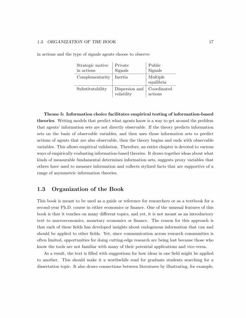
The following table summarizes some of the key interactions between strategic motives
1.3. ORGANIZATION OF THE BOOK 17
in actions and the type of signals agents choose to observe:
Strategic motive Private Publicin actions Signals Signals
Complementarity Inertia Multipleequilibria
Substitutability Dispersion and Coordinatedvolatility actions
Theme 5: Information choice facilitates empirical testing of information-based
theories. Writing models that predict what agents know is a way to get around the problem
that agents’ information sets are not directly observable. If the theory predicts information
sets on the basis of observable variables, and then uses those information sets to predict
actions of agents that are also observable, then the theory begins and ends with observable
variables. This allows empirical validation. Therefore, an entire chapter is devoted to various
ways of empirically evaluating information-based theories. It draws together ideas about what
kinds of measurable fundamental determines information sets, suggests proxy variables that
others have used to measure information and collects stylized facts that are supportive of a
range of asymmetric information theories.
1.3 Organization of the Book
This book is meant to be used as a guide or reference for researchers or as a textbook for a
second-year Ph.D. course in either economics or finance. One of the unusual features of this
book is that it touches on many diÆerent topics, and yet, it is not meant as an introductory
text to macroeconomics, monetary economics or finance. The reason for this approach is
that each of these fields has developed insights about endogenous information that can and
should be applied to other fields. Yet, since communication across research communities is
often limited, opportunities for doing cutting-edge research are being lost because those who
know the tools are not familiar with many of their potential applications and vice-versa.
As a result, the text is filled with suggestions for how ideas in one field might be applied
to another. This should make it a worthwhile read for graduate students searching for a
dissertation topic. It also draws connections between literatures by illustrating, for example,
18 CHAPTER 1. WHY STUDY INFORMATION CHOICE?
that the driving force in a monetary policy model is the same as that in a portfolio choice
model. These connections can help established researchers familiar with one area to quickly
have a strong intuitive grasp of the logic behind the models in another area. This makes the
chapters on monetary non-neutrality and business cycles perfectly appropriate for a class on
asset pricing and the portfolio choice chapter appropriate for a class on macroeconomics. The
ideas about how information choice can generate inertia are just as relevant for explaining
inertia in portfolio choices and the mechanism by which news about future productivity
aÆects current output can be used as the basis of an asset pricing model. Likewise, ideas
about how agents choose to trade financial securities can be used to explain puzzling features
of cross-country trade in goods and services. By drawing together insights from various
corners of macroeconomics and finance, I hope that this manuscript might advance work
in endogenous information by illuminating the possibilities for new applications of existing
tools and ultimately, helping to generate new insights about the role of information in the
aggregate economy.
Chapters 2 and 3 contain essential mathematical tools for understanding the material that
follows. The following two chapters consider a strategic game with many players. Stripping
away the details of any particular application makes the general themes that run through the
later models more transparent. Chapter 4 shows that when agents can choose information to
acquire before playing a strategic game, complementarity (substitutability) in actions typ-
ically generates complementarity (substitutability) in information choices. It also explains
why heterogeneous information can deliver unique predictions out of a model with coor-
dination motives where common knowledge would predict multiple equilibrium outcomes.
Chapter 5 illustrates how changing the amount of public information agents have access to
aÆects welfare diÆerently than changing the amount of private information.
Chapter 6 uses models from monetary economics to show how the combination of co-
ordination motives in price-setting and heterogeneous information creates strong inertia in
actions. When information choice is added to this setting, the coordination motive in infor-
mation strengthens this inertia. In chapter 7, the decision to invest in risky assets exhibits
substitutability instead of complementarity. As a result, agents want to acquire information
that is diÆerent from what other agents know. This leads them to hold diÆerent portfolios.
Chapter 8 also explores a setting where agents choose risky investments. But, rather than
focusing on the interaction between strategic motives in actions and information choices,
it introduces the idea of increasing returns in information. Neither the monetary nor the

1.3. ORGANIZATION OF THE BOOK 19
investment models considered a full production economy. Introducing an active role for in-
formation into such a general equilibrium setting creates new challenges. Chapter 9 explores
what model features allow information to act as an aggregate shock and create realistic
business cycle fluctuations or realistic asset price dynamics.
One of the reasons for writing a book that touches on so many applied topics is to oÆer
opportunities for the reader to take ideas and tools from one literature and bring them to
another. Therefore, each of the applied theory chapters (6 - 9) concludes with ideas about
how its tools or insights might be applied to answer other questions. Each particular project
may or may not be viable. The goal is to illustrate how the main concepts might be applied
more broadly so that the reader might be better able to formulate his or her own research
idea.
Of course, an applied theory paper is rarely considered complete without some empir-
ical support for its hypothesis. Therefore, chapter 10 is devoted to the subject of testing
information-based models. Finally, chapter 11 oÆers some concluding thoughts.
As information technology makes it possible to access a vast array of knowledge, con-
straints on what one can and cannot observe become less relevant. Yet, having access to
information is not the same as knowing it. Just like you can buy a textbook and not learn
its material, agents with access to information might not really acquire it in their working
memories. But putting information in our working memories – learning – is a choice. In other
words, information constraints are systematically being replaced with information choices.
It is such choices that this book seeks to understand.
Chapter 3
Measuring Information Flows
What is the feasible set of information choices? This is like asking what the feasible set of
labor-consumption choices is for a consumer in a production economy. In that setting, the
budget set depends on the relative price of each of the goods and of labor. But information
processing is something that individuals do for themselves. So it has no market price.1 Of
course, we could just assign a price to each signal. But how do we do that? Should a signal
that contains information about one risk be priced the same as a signal that contains some
information about many risks? Should a signal with one unit less variance cost $1 more,
or should a signal with one unit more precision cost $1 more, or neither? There is no right
answer to these questions. They are very important for the predictions of models based on
them. Any time you write down a model, you should think carefully about what its learning
technology means and why you chose it. Here are some examples of technologies that people
use.
3.1 Preliminaries
Why choose the variance instead of the mean? Investors can choose to see good or
bad news only if the information they are seeing is biased. An unbiased signal about x is x
plus mean-zero noise. The investor chooses how much information to get, not its content.
Consider the following analogy. Suppose there is an urn, one for each asset, that contains
1The idea that someone can process information for you and sell that service on a market is an idea wewill return to at the end. Set that idea aside for now.
29
30 CHAPTER 3. MEASURING INFORMATION FLOWS
balls with numbers printed on them. Those numbers are the true payoÆ of the asset, with
noise. The investor is choosing how many balls to draw from each urn. That determines the
precision of his signal. But he does not get to choose what is printed on any given ball. That
is the luck of the draw.
Choosing the signal variances is the same as choosing a variance of the posterior
belief. Recall that one of the rules for Bayesian updating with normal variables is that
the precision of the posterior belief is the sum of the precisions of the prior and the signals.
In general, there is one prior belief (with precision ß°1), but one or two signals. There is
one signal the agent chooses to observe; suppose it has precision ß°1¥ . In applications where
equilibrium prices (or quantities) also convey noisy information, there is a second signal which
is the information contained in prices; suppose it has precision ß°1p . The problem should be
set up so that prices are linear functions of the true state with normally distributed noise.
Otherwise, a non-linear filtering problem may render the problem intractable.
The precision of posterior beliefs is
bß°1 = ß°1 + ß°1p + ß°1
¥ .
The first term is information the agent is endowed with. The second term depends on how
much all other investors learn. Since the agent is one of a continuum, his actions alone do
not aÆect prices. Therefore, for every choice of ߥ, there is a unique bß that results. Because
of this one-to-one mapping, we can model the agent as choosing bß, instead of ߥ, taking ß
and ßp as given.
3.2 Entropy and Rational Inattention
The standard measure of the quantity of information in information theory is entropy (Cover
and Thomas, 1991). It is frequently used in econometrics and statistics and has been used
in economics to model limited information processing by individuals and to measure model
uncertainty.2 Entropy measures the amount of uncertainty in a random variable. It is also
2This is also referred to as a Shannon measure of information (Shannon, 1948). In econometrics, it is alog likelihood ratio. In statistics, it is a diÆerence of the prior and posterior distributions’ Kullback-Lieblerdistance from the truth. Mathematically, it is a Radon-Nikodym derivative. In robust control, it is thedistance between two models (Cagetti et al., 2002). It has been previously used in economics to model limitedmental processing ability (Radner and Van Zandt (2001) and Sims (2003)) and in representative investor
3.2. ENTROPY AND RATIONAL INATTENTION 31
used to measure the complexity of information transmitted. Following Sims (2003), this
section models the amount of information transmitted as the reduction in entropy achieved
by conditioning on that additional information (mutual information). The idea that economic
agents have limited ability to process information, or to pay attention, is often referred to as
rational inattention.
Entropy is a measure of the uncertainty of a random variable. It answers the question:
How much information is required, on average, to describe x with probability density function
p(·)?H(x) = °E[ln(p(x))]
= °X
x
[p(x) ln(p(x))] if p discrete
For a multivariate continuous distribution f
H(x) = °Z
f(x1, . . . , xn) ln(f(x1, . . . , xn))dx1, . . . , dxn
To make the idea of entropy more concrete, here are some examples.
• Constant: p(x) = 1 at x. At x, p(x) ln(p(x)) = 1 § 0, and p(x) = 0 everywhere else.
This is a zero entropy variable because if the variable is known to be a constant, no
information needs to be transmitted to know the value of the variable. I need a zero
length code to tell me that 2 = 2.
• Binomial: 2 points each with equal probability.
H = °(1
2ln(
1
2) +
1
2ln(
1
2)) = ° ln(
1
2) = ln(2)
Suppose we had a code that said if zero is observed, the variable takes on its first
value, if one is observed, it takes on its second value. Then, one zero or one must
be transmitted to reveal exactly the value of the variable. This is called one bit of
information. Bits are information flows, measured in base 2.
• Uniform: If x ª unif [0, a],
H(x) = °Z a
01/a ln(1/a)dx = ° ln(1/a) = ln(a)
models in finance (Peng, 2005).
32 CHAPTER 3. MEASURING INFORMATION FLOWS
Mutual information answers the question: How much do two variables x and y tell me
about each other? How much does knowing one reduce the entropy of the other?
I(x, y) = H(x)°H(x|y) (3.1)
The second term in the above expression is conditional entropy. It tells us: How much
information is required to describe x if y is already known?
H(x|y) = H(x, y)°H(y)
A useful property of mutual information is that it is symmetric:
I(x, y) = I(y, x).
What x tells you about y, y tells you about x.
Entropy and mutual information of normal variables Suppose that a variable x is
normally distributed: x ª N(µ,æ2). Then, it has entropy
H(x) =1
2ln(2ºeæ2). (3.2)
If x is an n£ 1 vector of normal variables, x ª N(µ,ß), then it has entropy
H(x) =1
2ln[(2ºe)n|ß|], (3.3)
where |ß| denotes the matrix determinant of ß.
Most models that use rational inattention in economics constrain the mutual information
that a set of signals can provide about the true state. With multi-dimensional, normally
distributed random variables, such a constraint takes the form
|bß| = exp (°2K)|ß| (3.4)
where bß is the posterior variance-covariance matrix, ß is the prior variance-covariance matrix
and K is a measure of mutual information, often called information capacity.
This constraint comes from the fact that an n-dimensional normal variable x ª N(µ,ß)
3.3. ADDITIVE COST IN SIGNAL PRECISION 33
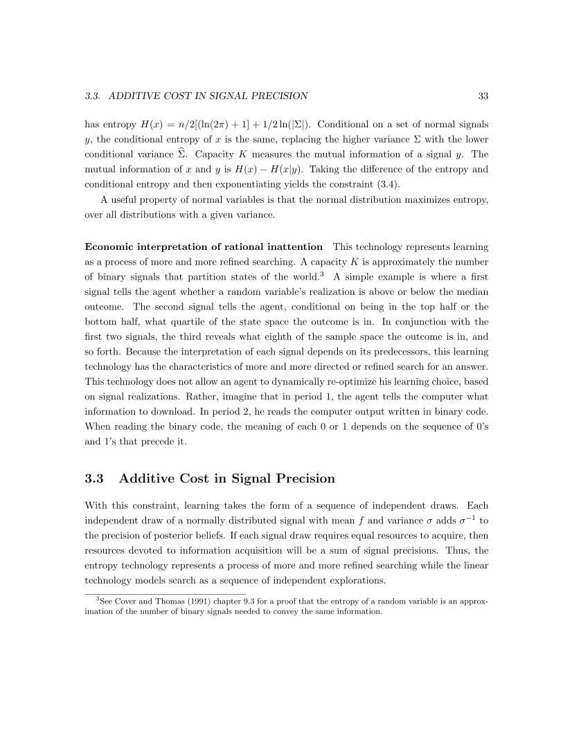
has entropy H(x) = n/2[(ln(2º) + 1] + 1/2 ln(|ß|). Conditional on a set of normal signals
y, the conditional entropy of x is the same, replacing the higher variance ß with the lower
conditional variance bß. Capacity K measures the mutual information of a signal y. The
mutual information of x and y is H(x) °H(x|y). Taking the diÆerence of the entropy and
conditional entropy and then exponentiating yields the constraint (3.4).
A useful property of normal variables is that the normal distribution maximizes entropy,
over all distributions with a given variance.
Economic interpretation of rational inattention This technology represents learning
as a process of more and more refined searching. A capacity K is approximately the number
of binary signals that partition states of the world.3 A simple example is where a first
signal tells the agent whether a random variable’s realization is above or below the median
outcome. The second signal tells the agent, conditional on being in the top half or the
bottom half, what quartile of the state space the outcome is in. In conjunction with the
first two signals, the third reveals what eighth of the sample space the outcome is in, and
so forth. Because the interpretation of each signal depends on its predecessors, this learning
technology has the characteristics of more and more directed or refined search for an answer.
This technology does not allow an agent to dynamically re-optimize his learning choice, based
on signal realizations. Rather, imagine that in period 1, the agent tells the computer what
information to download. In period 2, he reads the computer output written in binary code.
When reading the binary code, the meaning of each 0 or 1 depends on the sequence of 0’s
and 1’s that precede it.
3.3 Additive Cost in Signal Precision
With this constraint, learning takes the form of a sequence of independent draws. Each
independent draw of a normally distributed signal with mean f and variance æ adds æ°1 to
the precision of posterior beliefs. If each signal draw requires equal resources to acquire, then
resources devoted to information acquisition will be a sum of signal precisions. Thus, the
entropy technology represents a process of more and more refined searching while the linear
technology models search as a sequence of independent explorations.
3See Cover and Thomas (1991) chapter 9.3 for a proof that the entropy of a random variable is an approx-imation of the number of binary signals needed to convey the same information.
34 CHAPTER 3. MEASURING INFORMATION FLOWS
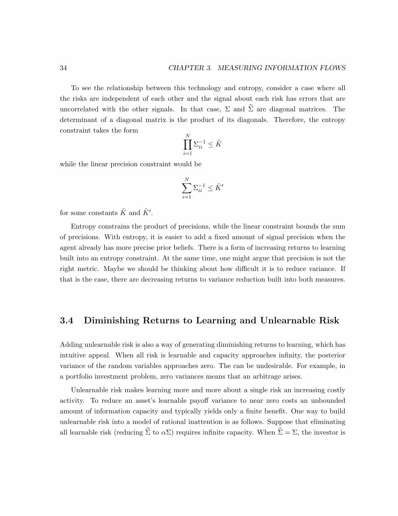
To see the relationship between this technology and entropy, consider a case where all
the risks are independent of each other and the signal about each risk has errors that are
uncorrelated with the other signals. In that case, ß and bß are diagonal matrices. The
determinant of a diagonal matrix is the product of its diagonals. Therefore, the entropy
constraint takes the formNY
i=1
ß°1ii ∑ K
while the linear precision constraint would be
NX
i=1
ß°1ii ∑ K 0
for some constants K and K 0.
Entropy constrains the product of precisions, while the linear constraint bounds the sum
of precisions. With entropy, it is easier to add a fixed amount of signal precision when the
agent already has more precise prior beliefs. There is a form of increasing returns to learning
built into an entropy constraint. At the same time, one might argue that precision is not the
right metric. Maybe we should be thinking about how di±cult it is to reduce variance. If
that is the case, there are decreasing returns to variance reduction built into both measures.
3.4 Diminishing Returns to Learning and Unlearnable Risk
Adding unlearnable risk is also a way of generating diminishing returns to learning, which has
intuitive appeal. When all risk is learnable and capacity approaches infinity, the posterior
variance of the random variables approaches zero. The can be undesirable. For example, in
a portfolio investment problem, zero variances means that an arbitrage arises.
Unlearnable risk makes learning more and more about a single risk an increasing costly
activity. To reduce an asset’s learnable payoÆ variance to near zero costs an unbounded
amount of information capacity and typically yields only a finite benefit. One way to build
unlearnable risk into a model of rational inattention is as follows. Suppose that eliminating
all learnable risk (reducing bß to Æß) requires infinite capacity. When bß = ß, the investor is
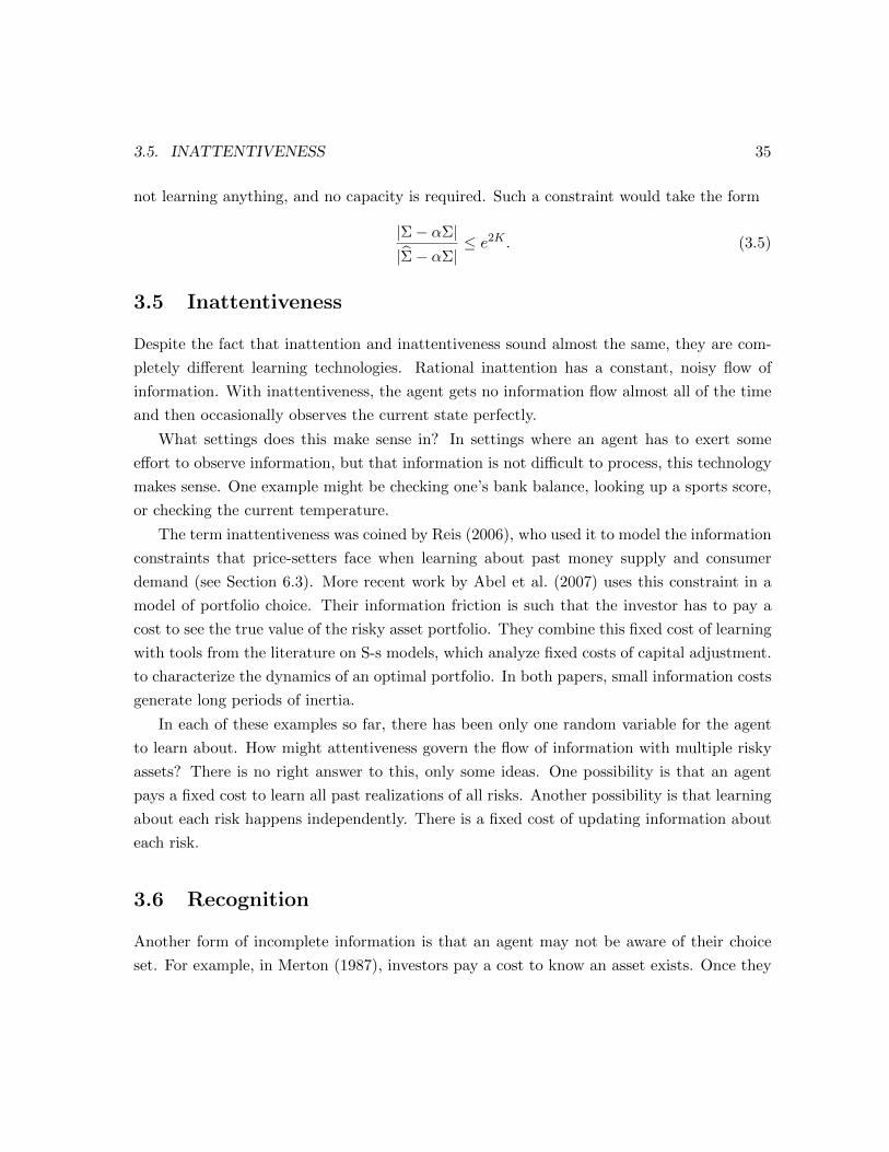
3.5. INATTENTIVENESS 35
not learning anything, and no capacity is required. Such a constraint would take the form
|ß° Æß||bß° Æß|
∑ e2K . (3.5)
3.5 Inattentiveness
Despite the fact that inattention and inattentiveness sound almost the same, they are com-
pletely diÆerent learning technologies. Rational inattention has a constant, noisy flow of
information. With inattentiveness, the agent gets no information flow almost all of the time
and then occasionally observes the current state perfectly.
What settings does this make sense in? In settings where an agent has to exert some
eÆort to observe information, but that information is not di±cult to process, this technology
makes sense. One example might be checking one’s bank balance, looking up a sports score,
or checking the current temperature.
The term inattentiveness was coined by Reis (2006), who used it to model the information
constraints that price-setters face when learning about past money supply and consumer
demand (see Section 6.3). More recent work by Abel et al. (2007) uses this constraint in a
model of portfolio choice. Their information friction is such that the investor has to pay a
cost to see the true value of the risky asset portfolio. They combine this fixed cost of learning
with tools from the literature on S-s models, which analyze fixed costs of capital adjustment.
to characterize the dynamics of an optimal portfolio. In both papers, small information costs
generate long periods of inertia.
In each of these examples so far, there has been only one random variable for the agent
to learn about. How might attentiveness govern the flow of information with multiple risky
assets? There is no right answer to this, only some ideas. One possibility is that an agent
pays a fixed cost to learn all past realizations of all risks. Another possibility is that learning
about each risk happens independently. There is a fixed cost of updating information about
each risk.
3.6 Recognition
Another form of incomplete information is that an agent may not be aware of their choice
set. For example, in Merton (1987), investors pay a cost to know an asset exists. Once they
36 CHAPTER 3. MEASURING INFORMATION FLOWS
recognize the asset, they can trade it costlessly. Merton calls this information “recognition.”
The concept is similar to that in search models where profitable trading opportunities exist
but agents cannot exploit these opportunities unless they pay a cost to search for them. The
diÆerence is that recognition is cumulative. An investor who becomes aware of an asset can
include it in his choice set forever after. An agent who searches can trade with counter-parties
that he encounters in that period. If he wants to trade in the next period, the agent must
search again.
Barber and Odean (2008) argue that when a stock is mentioned in the news, investors
become aware of it and that stock enters in their choice set. In other words, the market supply
of information aÆects individual investors’ attention allocation. They test this hypothesis by
measuring news coverage, trading volume and asset price changes.
Very little theoretical work has been done with this type of information constraint. In
addition to its applications in portfolio choice, it could be relevant for finding a job or hiring
workers, investing in or adopting a new technology or building trade relationships with foreign
importers or exporters.
3.7 Information Processing Frictions
Another kind of information friction, similar to incomplete information, is the failure to
process observed information. For example, Hirschleifer et al. (2005) assume that all agents
observe whether or not a firm discloses a signal. But only a fraction of agents who observe
non-disclosure infer correctly that non-disclosing firms have bad news.
Such assumptions blur the line between information frictions and non-rational behavior.
Yet, there is a close relationship between information flow constraints and computational
complexity constraints. In particular, entropy can be interpreted as either kind of constraint.
See Cover and Thomas (1991) for more on measuring computational complexity. See Rad-
ner and Van Zandt (2001) for a model that uses an entropy-based information processing
constraint to determine the optimal size of a firm.
This kind of assumption may be useful in avoiding problems that arise in equilibrium
models. For example, agents need to know prices to satisfy their budget constraint. Yet,
prices may contain information that allows agents to infer what others know. In such a
setting, an information processing constraint can preserve information heterogeneity, whereas
costly information acquisition might not.
3.8. LEARNING WHEN OUTCOMES ARE CORRELATED 37
3.8 Learning When Outcomes Are Correlated
Suppose asset A and asset B have payoÆs that are unknown, but positively correlated. An
investors observes a signal about asset A, suggesting that its payoÆ is likely to be high.
Knowing that the payoÆ of asset B is positively correlated, the investor infers that B’s payoÆ
is also likely to be high. How can we describe the information content of this signal? It is a
signal about asset A’s payoÆ, that contains information about B’s payoÆ as well. The first
objective of this section is to put forth a language for describing the information content of
signals when risks are correlated.
The second issue this section addresses is about how to model information choice. Should
agents choose the entire covariance structure of the signals they observe, or should we restrict
their choice set and allow then to obtain only signals about risks, with a given covariance
structure? This question arises with many of the learning technologies we have described.
(However, inattentiveness is somewhat immune to this problem because it dictates a choice
of when to set the variance of all unknown state variables equal to zero.) Any problem where
signal variances are chosen and multiple risks are present is confronted with this question.
Correlated outcomes and orthogonal risk factors. If a signal can pertain to multiple
assets, we need a language to describe what information each signal has. One way to do
this is to describe signals according to how much information they contain about each the
realization of each principal component.
Suppose we have an N £ 1 random variable f ª N(µ,ß), where ß, the prior variance-
covariance matrix, is not a diagonal matrix. Thus, the realizations of the N elements of f
are correlated. An eigen-decomposition splits ß into a diagonal eigenvalue matrix §, and an
eigenvector matrix °:
ß = °§°0. (3.6)
(See appendix 3.10 for more information and rules about eigen-decompositions.) The §i’s are
the variances of each principal component, or risk factor, i. The ith column of ° (denoted °i)
gives the loadings of each random variable on the ith principal component. Since realizations
of principal components f 0°i are independent of each other, a signal that is about principal
component i would contain no information about principal component j. This allows an
unambiguous description of the information content of a signal.
What we are doing is taking some correlated random variables and forming linear combi-
38 CHAPTER 3. MEASURING INFORMATION FLOWS
nations of those variables, such that the linear combinations are independent of each other.
Take an example where the variables are the payoÆs of risky assets. The principal compo-
nents would then be linear combinations of assets – call them portfolios or synthetic assets
– that one can learn about, buy and price, just as if they were the underlying assets. Such
synthetic assets are also referred to as Arrow-Debreu securities. The reason we want to work
with these synthetic assets is that their payoÆs are independent of each other. Principal
components analysis is frequently used in the portfolio literature (Ross, 1976). Principal
components could represent business cycle risk, industry-specific risk, or firm-specific risk.
As long as there are no redundant assets (i.e. the variance-covariance matrix of payoÆs is
full-rank), rewriting the problem and solving it in terms of the independent synthetic assets
can be done without loss of generality.
Thus, after transforming the problem with our eigen-decomposition, we can proceed and
solve the model, as if assets were independent. If you can solve the a model with independent
risks, you can just as easily solve the correlated risk version as well.
Should signals about independent risks be independent? An assumption that a sig-
nal about any principal component i does not contain information about any other principal
components is not without loss of generality. To be clear, this assumption does not rule out
learning about many risks. It does rule out signals with correlated information about risks
that are independent. Here is a simple example of what the assumption prohibits: If rain
in Delhi and the supply of Norwegian oil are independent risks, the investor cannot choose
to observe a signal that is the diÆerence between the millions of barrels of Norwegian oil
pumped and the centimeters of rain in Delhi. He can learn about oil and rain separately and
construct that diÆerence. But he cannot learn the diÆerence without knowing the separate
components. If we learned the diÆerence, such a signal would induce positive correlation be-
tween his beliefs about oil and rainfall. For example, if he believed that oil will be abundant
and that the diÆerence between oil and rainfall is small, then he must believe that rainfall
will be abundant as well. Since such a signal does not preserve independence of independent
risks, the proposed assumption would prohibit an investor from choosing to observe it.
The mathematical intuition for the independent signal assumption is the following: For
a normally-distributed signal, ¥i ¥ °0if + ≤i, the signal noise ≤i must be uncorrelated across
components i. In other words, the n£1 vector of noise terms for each principal component is
distributed ≤ ª N(0,§¥), where §¥ is a diagonal matrix. The assumption that §¥ is diagonal
3.8. LEARNING WHEN OUTCOMES ARE CORRELATED 39
simplifies the problem greatly because it reduces its dimensionality. It allows us to only
keep track of the n diagonal entries of §¥, rather than the n(n + 1)/2 distinct entries of a
symmetric variance covariance matrix. But the reduced number of choice variables is clearly
a restriction on the problem.
Equivalently, the signal could be about the underlying random variable, as long as the
signal noise has the same risk structure as the random variable itself. Define ∫ ¥ °¥. Then
∫|f has mean °E[¥|f ] = °°0f . Since eigenvectors of symmetric matrices are idempotent
by construction, °°0 = I and E[∫|f ] = f . Thus, ∫ is a signal about the variable f . Since
multiplication by ° is a linear operation, ∫ is normally distributed, ∫|f ª N(f,°§¥°0). Notice
that the variance of the signal noise in ∫ has the same eigenvectors (same risk structure) as
the prior beliefs about f .
If we do make the assumption that signals about principal components are independent,
then the variance of posterior beliefs has the same eigenvectors as prior beliefs. If f |¥ ªN(µ, bß), then bß = °§°0. (The proof of this is left as an exercise.) The diagonal matrix §
contains the posterior variance of beliefs about each risk factor. Learning about risk i lowers
§i relative to the prior variance §i. The decrease in risk factor variance §i,i ° §i,i captures
how much an agent learned about risk i.
In the asset example, if we assume that signal errors have the same risk structure (their
variance has the same eigenvectors) as asset payoÆs, then the synthetic asset payoÆs are con-
ditionally and unconditionally independent. In other words, the prior and posterior variance-
covariance matrices of the synthetic asset payoÆs are diagonal.
When using information flow measures to quantify information acquisition or research
eÆort, uncorrelated signals may be a realistic assumption. Acquiring information about oil
is a separate task from acquiring information about rainfall. Perhaps someone can learn
about the diÆerence or oil and rain, if someone else constructs that joint signal for them.
But then who constructs the signal and how they price it become important questions and
should be part of the model. Sims (2006) disagrees; he thinks of rational inattention as
describing a setting where complete and perfect information is available for any agent to
observe. The agent just cannot observe all the information and must choose the optimal
information to observe. If optimized information flows involve constructing correlated signals
about independent events, so be it. Which procedure most resembles how economic decision
makers learn is an open question.
If you are willing to assume that signals about uncorrelated principal components have
40 CHAPTER 3. MEASURING INFORMATION FLOWS
uncorrelated signal errors, then you can solve your problem as if all your assets and signals are
independent. Once you have a solution for the independent (synthetic) asset and independent
signal case, just pre-multiply the price and quantity vectors by the eigenvector matrix °0 to
get the price and quantity vectors for the underlying correlated assets.
3.9 What is the Right Learning Technology?
Does learning have increasing or decreasing returns? Does it have to apply to all the stochastic
variables in the model? Are people like computers in their processing abilities? These are
open questions in the literature. Probably their answers depend on the context.
Below are some suggestions for how to evaluate a learning technology
• Experimental evidence
• Adopt a standard. For example, there are many ways one might represent goods pro-
duction; yet, the profession has settled on the Cobb-Douglas function as an industry
standard. This literature may settle on a few key properties that a reasonable informa-
tion production function should have. For goods production, that feature was a stable
share of income paid to labor and to capital. One possible standard for information
production is scale neutrality, discussed below.
• For now, the best we can do is to justify our model assumptions with model results.
If putting in a diÆerent learning technology would make the model predict unrealistic
outcomes, then perhaps another learning technology is in order. The problem with this
answer is that if one learning technology fails to explain a phenomenon, it could also
be because learning is not a key part of the explanation. It is important to distinguish
between facts that justify your assumptions and independent facts that you use to
evaluate the model’s explanation.
One of the drawbacks to using the additive precision measure of information is that it is
not scale neutral. For example, the definition of what constitutes one share of an asset will
change the feasible set of signals. Take a share of an asset with payoÆ f ª N(µ,æ) and split
it into 2 shares of a new asset, each with payoÆ f/2. The new asset has payoÆs with 1/2 the
standard deviation and 1/4 the variance. The prior precision of information about its payoÆ
is therefore 4æ°1.
3.10. APPENDIX: MATRIX ALGEBRA AND EIGEN-DECOMPOSITIONS 41
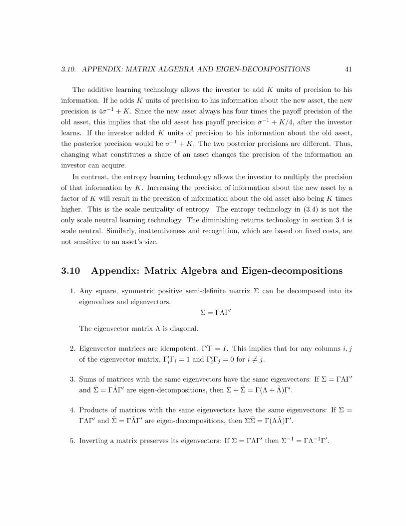
The additive learning technology allows the investor to add K units of precision to his
information. If he adds K units of precision to his information about the new asset, the new
precision is 4æ°1 +K. Since the new asset always has four times the payoÆ precision of the
old asset, this implies that the old asset has payoÆ precision æ°1 + K/4, after the investor
learns. If the investor added K units of precision to his information about the old asset,
the posterior precision would be æ°1 +K. The two posterior precisions are diÆerent. Thus,
changing what constitutes a share of an asset changes the precision of the information an
investor can acquire.
In contrast, the entropy learning technology allows the investor to multiply the precision
of that information by K. Increasing the precision of information about the new asset by a
factor of K will result in the precision of information about the old asset also being K times
higher. This is the scale neutrality of entropy. The entropy technology in (3.4) is not the
only scale neutral learning technology. The diminishing returns technology in section 3.4 is
scale neutral. Similarly, inattentiveness and recognition, which are based on fixed costs, are
not sensitive to an asset’s size.
3.10 Appendix: Matrix Algebra and Eigen-decompositions
1. Any square, symmetric positive semi-definite matrix ß can be decomposed into its
eigenvalues and eigenvectors.
ß = °§°0
The eigenvector matrix § is diagonal.
2. Eigenvector matrices are idempotent: °0° = I. This implies that for any columns i, j
of the eigenvector matrix, °0i°i = 1 and °0
i°j = 0 for i 6= j.
3. Sums of matrices with the same eigenvectors have the same eigenvectors: If ß = °§°0
and ß = °§°0 are eigen-decompositions, then ß+ ß = °(§+ §)°0.
4. Products of matrices with the same eigenvectors have the same eigenvectors: If ß =
°§°0 and ß = °§°0 are eigen-decompositions, then ßß = °(§§)°0.
5. Inverting a matrix preserves its eigenvectors: If ß = °§°0 then ß°1 = °§°1°0.
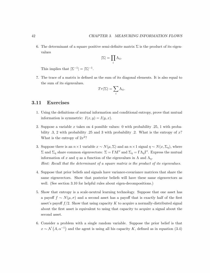
42 CHAPTER 3. MEASURING INFORMATION FLOWS
6. The determinant of a square positive semi-definite matrix ß is the product of its eigen-
values
|ß| =Y
i
§ii.
This implies that |ß°1| = |ß|°1.
7. The trace of a matrix is defined as the sum of its diagonal elements. It is also equal to
the sum of its eigenvalues.
Tr(ß) =X
i
§ii.
3.11 Exercises
1. Using the definitions of mutual information and conditional entropy, prove that mutual
information is symmetric: I(x, y) = I(y, x).
2. Suppose a variable x takes on 4 possible values: 0 with probability .25, 1 with proba-
bility .3, 2 with probability .25 and 3 with probability .2. What is the entropy of x?
What is the entropy of 2x2?
3. Suppose there is an n£1 variable x ª N(µ,ß) and an n£1 signal ¥ ª N(x,ߥ), where
ß and ߥ share common eigenvectors: ß = °§°0 and ߥ = °§¥°0. Express the mutual
information of x and ¥ as a function of the eigenvalues in § and §¥.
Hint: Recall that the determinant of a square matrix is the product of its eigenvalues.
4. Suppose that prior beliefs and signals have variance-covariance matrices that share the
same eigenvectors. Show that posterior beliefs will have these same eigenvectors as
well. (See section 3.10 for helpful rules about eigen-decompositions.)
5. Show that entropy is a scale-neutral learning technology. Suppose that one asset has
a payoÆ f ª N(µ,æ) and a second asset has a payoÆ that is exactly half of the first
asset’s payoÆ f/2. Show that using capacity K to acquire a normally-distributed signal
about the first asset is equivalent to using that capacity to acquire a signal about the
second asset.
6. Consider a problem with a single random variable. Suppose the prior belief is that
x ª N°A,Æ°1
¢and the agent is using all his capacity K, defined as in equation (3.4)

3.11. EXERCISES 43
to observe x. What is the precision of that signal?
7. Suppose the prior belief is that x ª N°A,Æ°1
¢and the agent has capacity K which
he uses to process (public) information contained in prices, p, and a private signal. It
is a common knowledge that p ª N°x,Ø°1
¢. What fraction of his capacity does the
agent have to use to process information contained in prices? How precise a private
signal can he observe with the remaining capacity?