Focus University of Wisconsin–Madison Institute for Research on Poverty

Volume 22

Number 2

Summer 2002

ISSN: 0195–5705

Why were the nineties so good? Could it happen again? Robert M. Solow

Robert M. Solow is Institute Professor of Economics Emeritus at Massachusetts Institute of Technology. This article is adapted from the Robert J. Lampman Memorial Lecture that he delivered in Madison in June 2001.

The research project I sketch here had its origin in some facts about the performance of the U.S. economy. During

Why were the nineties so good? Could it happen again? 1

The right (soft) stuff: Qualitative methods and the study of welfare reform 8

Marriage and fatherhood

Expectations about marriage among unmarried parents: New evidence from the Fragile Families Study 13

The economic circumstances of fathers with children on W-2 19

The life circumstances of African American fathers with children on W-2: An ethnographic inquiry 25

Children’s living arrangements after divorce: How stable is joint physical custody? 31

IRP Visiting Scholars, 2002 32

Including the poor in the political community 34

Evaluation of State TANF Programs: An IRP Confer-ence, April 2002

TANF programs in nine states: Incentives, assistance, and obligation 36

TANF impact evaluation strategies in nine states 41

Perspectives of researchers and federal officials: A panel session 48

Income Volatility and the Implications for Food Assistance Programs: A Conference of IRP and the Economic Research Service of the U.S. Department of Agriculture, May 2002

Income volatility and the implications for food assistance programs 56

The role of food stamps in stabilizing income and consumption 62

Income volatility and household consumption: The impact of food assistance programs 63

Short recertification periods in the U.S. Food Stamp Program: Causes and consequences 64

Food Stamps and the elderly: Why is participation so low? 66

Gateways into the Food Stamp Program 67

WIC eligibility and participation 68

The correlates and consequences of welfare exit and entry: Evidence from the Three-City Study 70

Measuring the well-being of the poor using income and consumption 72

the five years 1995–2000, the U.S. economy grew faster, maintained a lower unemployment rate, and experienced less inflation than in the quarter-century from 1970 to 1995 (Table 1). No serious macroeconomist that I know would have thought in 1990 that the U.S. economy could go through a five-year period of rapid growth, drive the unemployment rate steadily down to 4 percent in the fifth year, and still find the inflation rate steady or falling. This would have been regarded as an impossibly optimistic scenario; and I would have agreed.

2

Yet the years 1995–2000 were not quite an economic miracle, as Table 1 also shows. The decade of the 1960s exhibited equally good performance. By the end of the 1960s, however, the Vietnam War was driving the U.S. economy. We now think of that period as the prelude to the inflation of the 1970s. So far, the prosperity of the 1990s does not seem to have that consequence. So we are talking about a remarkable five years.

Two lively and interesting New York foundations—the Russell Sage Foundation and the Century Foundation— were provoked to try to understand this surprising epi-sode. Their interest was not purely scientific. They re-membered that “full employment” had once been a primary goal of national economic policy. In those days, that meant a state of affairs in which inflation did not threaten, and the measured unemployment rate was very close to the inevitable amount of frictional unemploy-ment.1

Full employment, in that sense, was expected to bring with it many social benefits: lower crime, better health, improved family structure, wider access to education. The foundations were aware that over the years, the goals of macroeconomic policy had receded to the acceptance of unemployment rates much higher than the frictional level; the avoidance not merely of inflation but of accel-erating inflation had become the overriding objective of macro-policy. Now suddenly the United States had achieved something very like the old ideal of “full em-

ployment.” They wondered what factors had permitted this to happen, and whether such conditions could be sustained as a normal outcome. Nothing could be more important for the well-being of the least advantaged part of the population. Even those who are necessarily out of the labor force profit from full employment, if only be-cause governments find themselves flush with revenue and better able to support transfer payments relatively painlessly.

The two foundations asked Professor Alan Krueger of Princeton University and me to design and organize a research project that explored the causes and likely per-manence of these changed economic relationships. The findings from this research have been published as a volume, The Roaring Nineties: Can Full Employment Be Sustained? by the Russell Sage Foundation (see box, p. 4). It did not occur to me until this project was well under way that it had an unusual aspect. We were trying to understand a single episode in one country. One might think that there is nothing special about that: we just have to see how it fits into some more general “covering” theory. But that is much too simple. Any event that is singled out as an “episode” is almost by definition atypi-cal or peculiar. Otherwise it would not be dignified with that label. There are always exogenous events occurring, and it is rarely clear how they are to be integrated into a coherent story about the episode. Except very rarely, one cannot intelligently compare one episode with another, because the other will have been influenced by a different collection of exogenous events and different historical antecedents. After all, it is over two hundred years since 1789, and right now someone, somewhere, is writing another book about the causes of the French Revolution.

It was not our goal to reform macroeconomic theory, so we approached our question in the vocabulary of the theoretical consensus of the time: roughly speaking, the expectations-augmented, accelerationist Phillips curve (although I, personally, have always had my doubts about that theory). This consensus view presumed the effective-ness of two constraints on macroeconomic performance. (For an explanation of the Phillips curve, see box, p. 3.)

First, the trend growth rate of potential GDP in the United States was widely believed to be somewhere near 2.0–2.5 percent a year, and to be limited mainly by the slow growth of productivity, at a rate of 1.0–1.5 percent a year. Of course, the economy could grow faster than that after a

The Robert J. Lampman Memorial Lecture Series

Established to honor Robert Lampman, professor of economics and founding director and guiding spirit of IRP until his death in 1997, the lecture series is organized by IRP in conjunction with the University of Wisconsin–Madison’s Department of Economics. A fund has been established to support an annual lecture by a distinguished scholar on the topics to which Lampman devoted his intellectual career: poverty and the distribu-tion of income and wealth. This memorial has been established by the Lampman family, with the help of the University of Wisconsin Founda-tion. The series offers a special opportunity to maintain and nurture interest in poverty research among the academic community and members of the public. The Institute extends its deep ap-preciation to the Lampman family and other do-nors for making this opportunity possible.

The 2002 Lampman Lecturer is Eugene Smolensky, Professor of Public Policy at the Uni-versity of California, Berkeley. Other Lampman Lecturers have included Sheldon Danziger, Ed-ward M. Gramlich, and Angus Deaton.

Table 1 Economic Performance, by Decade, 1960–2000

1990s (second half) 1980s 1970s 1960s

Real GDP growth (%) 3.2 (4.0) 3.0 3.3 4.4

Unemployment rate (%) 5.8 (5.0) 7.3 6.2 4.8

Inflation rate (%) 2.9 (2.4) 5.1 7.4 2.5

3

tion? Must 1995–2000 be regarded as a one-time, nonrepeatable episode, a single piece of good luck, or have the macroeconomic rules changed more nearly per-manently? Are there policy choices that would make it possible to sustain the performance of 1995–2000 for the long term?

Because we wanted to know how best to sustain a high- employment economy, we assigned each of the topics to be covered to a team consisting of (at least) one microeconomically and one macroeconomically oriented person, wherever it seemed reasonable to do so. Part of the exercise was to determine whether this single episode falls easily into some standard category, although, as I have noted, there are bound to be historical peculiarities, chance events, one-time deviations from the norm, and other such factors whose influence is hard to understand and evaluate. Certainty about conclusions was probably too much to expect, and that will be seen to be the case here. But we can provide a better sense of where to look to understand what made the decade so successful.

To begin with, we decided to take the faster growth of potential output for granted, as an exogenous event.2 We chose to focus on the employment (or unemployment) story itself, which is complicated enough. The research as we conceived it consists primarily of investigations into one aspect or another of the labor market. In every case, it is the macroeconomic implications of labor market devel-

The Phillips curve and inflation

The Phillips curve is named for its originator, New Zealand economist A. W. Phillips, whose studies of unemployment and the rate of inflation in Britain between 1861 and 1957 led him to conclude that there was a predictable inverse relationship between the two. The “Phillips curve” graphically describes this observation: Whenever unemployment is low, inflation tends to be high. Whenever unemployment is high, inflation tends to be low.

In the 1970s, however, higher inflation in the United States was associated with higher—not lower—unemploy-ment. The average inflation rate rose from about 2.5 percent in the 1960s to about 7 percent in the 1970s, and average unemployment from about 4.75 percent to about 6 percent, calling into question the validity of the relationship posited in the Phillips curve and raising serious issues for policymakers. If the relationship between unemployment and inflation was not predictable in the way the Phillips curve assumed, then the inflation cost of targeting a particular unemployment rate was not clearly identifiable. As Robert Solow discusses in the accompanying article, the years 1995–2000 also challenge the conventional understanding of the inflation- unemployment relationship.

Inflation is considered low or high relative to the expected rate of inflation. Unemployment is considered low or high relative to the so-called “natural rate” of unemployment, a concept first presented in 1968 by Milton Friedman in his Presidential Address to the American Economic Association. In Friedman’s view, which is accepted by many macroeconomists, the “natural rate” is determined by the microeconomic structure of labor markets and household and firm decisions affecting labor supply and demand. Many, however, prefer to call this the “nonaccelerating inflation rate of unemployment” (NAIRU), because unlike the term “natural rate” it does not suggest an unemployment rate from which the economy may temporarily shift but to which it inevitably returns, which policy cannot alter, and which is somehow socially optimal.

Sources: Federal Reserve Bank of San Francisco, Economic Letter 98-28, “The Natural Rate, NAIRU, and Monetary Policy,” <http://www.frbsf.org/econrsrch/wklyltr98/el98-28.html>; J. Bradford Delong, “The Phillips Curve,” <http://www.j-bradford-delong.net/multimedia/PCurve1.html>; Kevin D. Hoover, “The Phillips Curve,” <http://www.econlib.org/library/Enc/PhillipsCurve.html>.

recession had opened up some slack that could be elimi-nated in the next upswing. But that could be only a tempo-rary, unsustainable burst.

Second, a good sign that the economy had reached its potential output, and was thus on the verge of tipping over into ever-increasing inflation, would be a reduction of the unemployment rate to 6.0–6.5 percent. This was widely believed to be the “inflation-safe” unemployment rate in the United States (the nonaccelerating inflation rate of unemployment, or NAIRU, what economists call the natural rate). The inflation-safe unemployment rate does what it says—it looks only for an unemployment rate just high enough to keep inflation from worsening. One does not have to accept a whole theory of a “natural rate of unemployment”—though most macroeconomists do so—to believe that too much pressure of the economy against its productive capacity (measured, for instance, by too low an employment rate) would cause wages and prices to rise unacceptably. Because I have some doubts about the accompanying theory, I shall consistently call this the “neutral rate.”

The 1995–2000 episode plainly violated both these folk- beliefs emphatically. Were there identifiable changes in economic institutions or behavior patterns that relaxed those earlier constraints or made them go away? Or were there instead some favorable random events that im-proved economic performance beyond normal expecta-

4

opments that are the main concern. Our basic question is: Why was the inflation-safe unemployment rate so low between 1995 and 2000? In this article I have space only to glance briefly at the most explicitly macroeconomic analyses—they are the first three chapters of our book— and at some of the interesting questions and ambiguities that emerge.

Even to ask that question implies that the neutral rate of unemployment is not constant from place to place or from time to time. An important first step toward an answer is provided by a careful econometric analysis of the period

since 1960 by Douglas Staiger, James Stock, and Mark Watson, in which they incorporate one very substantial element of flexibility by calculating a “trend unemploy-ment rate” that is essentially a moving average of the series of observed unemployment rates. The rate they construct reaches a minimum of somewhat over 4 percent in 1970 and a maximum of nearly 8 percent around 1980. It then falls steadily and dramatically until it is below 5 percent in 2000. Estimating a Phillips curve with a neutral rate that is not constrained to be constant for long inter-vals, they find that the inflation-safe unemployment rate so estimated is always very close to the trend unemploy-

The Roaring Nineties: Can Full Employment Be Sustained?

Introduction Alan B. Krueger and Robert M. Solow

Part I Macroeconomic Perspectives

1 Prices, Wages, and the U.S. Nairu in the 1990s Douglas Staiger, James H. Stock, and Mark W. Watson

2 Productivity Growth and the Phillips Curve Laurence Ball and Robert Moffitt

3 The Fabulous Decade: Macroeconomic Lessons from the 1990s Alan S. Blinder and Janet L. Yellen

Part II Flexible, Open Labor Markets

4 Comparative Analysis of Labor Market Outcomes: Lessons for the United States from International Long-run Evidence

Giuseppe Bertola, Francine D. Blau, and Lawrence M. Kahn

5 Have the New Human-Resource Management Practices Lowered the Sustainable Unemployment Rate? Jessica Cohen, William T. Dickens, and Adam Posen

6 The Effects of Growing International Trade on the U.S. Labor Market George Johnson and Matthew J. Slaughter

Part III Increasing Labor Supplies and Their Limits

7 Labor and the Sustainability of Output and Productivity Growth Rebecca M. Blank and Matthew D. Shapiro

8 Changes in Unemployment Duration and Labor-Force Attachment Katharine G. Abraham and Robert Shimer

9 The Sputtering Labor Force of the Twenty-first Century: Can Social Policy Help? David T. Ellwood

Part IV The Benefits and Pitfalls of Tight Labor Markets

10 Another Look at Whether a Rising Tide Lifts All Boats James R. Hines, Jr., Hilary W. Hoynes, and Alan B. Krueger

11 Rising Productivity and Falling Unemployment: Can the U.S. Experience Be Sustained and Replicated? Lisa M. Lynch and Stephen J. Nickell

Copublished with the Century Foundation, January 2002. Available from: Russell Sage Foundation | 112 East 64th Street | New York, NY 10021

Voice: 212.750.6000 | Fax: 212.371.4761 | info@rsage.org

5

ment rate. (To a natural skeptic like me, it is too close for comfort; but that is what the econometrics tells us.) The implication is that the very good years 1995–2000 could afford to be so good because both the trend rate and the neutral rate were below where they had been in the 1970s and 1980s, and were still falling. The authors argue that we need invoke no other causal factor—no exogenous events or “good luck” in the form of favorable supply shocks that happened to counteract any tendency for price inflation to take off.

Here there is a very important ambiguity to be resolved. Alan Blinder and Janet Yellen, who were policy insiders during this period (both served on the Federal Reserve Board and in the Council of Economic Advisers during the Clinton administration) disagree with Staiger and his colleagues. They attach quite a lot of importance to favor-able supply shocks, in particular the surge in productivity growth that I have already mentioned.

On the wage side, they point to the deceleration of em-ployers’ benefit costs. The main components were the effect on the costs of employer-provided health care of the shift to “managed care” and the boom in the stock market that enabled many employers to reduce or elimi-nate current contributions to pension funds (because ris-ing stock prices increased the value of the funds and kept them actuarially sound). On the price side, they empha-size the appreciation of the dollar after 1995, the result-ing fall in the prices of imports other than oil, and then the drastic drop in the world oil price, which fell by half between late 1996 and early 1999. Finally, adjustments in

the way the Consumer Price Index measures product quality correctly lowered the reported rate of inflation. Blinder and Yellen argue that these supply shocks explain the drop in inflation, which otherwise would have risen into the 5 percent range by the end of 1998, according to some econometric models.3

This sounds as if we can account for the combination of low unemployment and low inflation twice over, once without supply shocks and once with nothing but supply shocks. Then the puzzle about 1995–2000 would not be to understand why inflation was so low, but why it was not even lower. I am not sure that I fully understand how to deal with this situation. It is part of the intrinsic diffi-culty of trying to “explain” a single historical episode.

But one formulation that avoids any inconsistency is to realize that favorable supply shocks actually lower the inflation-safe unemployment rate. When the price of oil is falling, for example, it is possible to live with a tighter, more fully employed economy, without overall inflation picking up. Rising wage costs could be offset by falling fringe-benefit and energy costs, leaving prices more or less insulated. Then if opportunistic policy (or chance, for that matter) keeps the economy close to the new, lower, safe unemployment rate, the observed trend unem-ployment rate will also be lower. Then these two different explanations could really be two ways of doing the same calculation.

The apparent fall in the inflation-safe unemployment rate to a very low figure by the end of the 1990s is a fact—I

Figure 1. Trend unemployment and productivity growth, 1960–2000.

0

1

2

3

4

5

6

7

8

9

1960 1965 1970 1975 1980 1985 1990 1995 2000

Year

Per

cen

tUnemployment Rate Trend

Productivity Growth Trend

6

think it is a fact—in search of a theory. And Staiger and his colleagues offer us another fact that offers a broad hint about a possible story. Figure 1 shows two trends— the smoothed unemployment rate trend already discussed and a similarly smoothed trend rate for productivity growth. The negative correlation between the two leaps to the eye, with productivity growth apparently leading un-employment by a little at the turning points.

Another piece of our project, by Laurence Ball and Rob-ert Moffitt, joins this observation to a story that associ-ates fast productivity growth with slow cost growth, and therefore with low inflation. (Blinder and Yellen list the surge in productivity growth as perhaps the most impor-tant favorable supply shock.) They start from a fairly conventional “real-wage” Phillips curve. If productivity were not increasing, the growth of real wages would depend negatively on the unemployment rate (i.e., as the unemployment rate falls, wages rise). But plausibly, if productivity is rising, workers will aim at a real wage that grows with productivity, not necessarily year by year, but on the average. Employers will be driven by competition to go along. If you add to this story the same old rule for prices—a more or less constant markup on unit labor costs—it is easily seen that the rate of inflation is inde-pendent of the rate of productivity growth. This is be-cause productivity growth is fully offset by wage in-creases; there is nothing left over to affect inflation. Faster or slower productivity growth would then be ac-companied by faster or slower wage increases, leaving inflation untouched.

Now Ball and Moffitt introduce a new concept. They want to model an inertial or persistent component in workers’ wage aspirations. They do so by defining an “aspiration” standard for real-wage growth; they choose to make it a weighted average of past rates of real-wage growth. Wage increases are habit-forming, both for work-ers and employers. The conventional model says that what drives real wages upward is the growth of productiv-ity; Ball and Moffitt say that real wages are driven up-ward by productivity growth and customary real wage growth. In a steady state, real wages grow in line with productivity; then the aspiration standard will grow at the same rate and so will any average of the two. In that case, the refinement of the aspiration standard makes no differ-ence, but in all other cases it does, and in the historical case that we are examining it makes just the right differ-ence.

Here is one plausible story. (There are others, and they are discussed in the book.) Start from a steady state and imagine that productivity accelerates, as it did in 1995– 2000. Faster productivity growth feeds into real wages, but not one-for-one; in fact, it is only about one-half-to- one in the early stages. This is because the aspiration standard is sluggish; it looks back over past wage in-creases. So real wages lag behind productivity, unit labor costs slow down or fall, and inflation does the same. As

long as this gap lasts, it can be used either to run the economy at a lower unemployment rate with the old rate of inflation, or at the old unemployment rate with lower inflation. In other words, the “safe” unemployment rate is temporarily lower.

The implication for our period is that the surprise accel-eration of productivity beginning in 1995, by running ahead of the aspiration standard, allowed unemployment to fall while inflation continued to hover around 2 per-cent. A conventional Phillips curve would have translated the low unemployment rate—which fell from an already dangerous 6 percent at the beginning of 1995 to 4 percent at the end of 2000—into a forecast of runaway inflation. A forecast using Ball and Moffitt’s refinement gets the inflation forecast essentially right, and without bias.

To sum up: In our study, we formulated the basic question in the way current mainstream macroeconomics would frame it. How was it possible in the years 1995–2000 to reconcile low and falling unemployment with low and stable inflation? In the standard jargon, how did the NAIRU—the inflation-safe unemployment rate, what I am calling the neutral rate—get to be as low as perhaps 4 percent, when only a few years earlier it was generally thought to be 6 percent or even higher?

The possibility emerges that the fall of the neutral rate was a stage in a longer-term process. The careful estimate of Staiger and his colleagues suggests that the neutral rate peaked near 8 percent in 1980 and then fell fairly smoothly to near 4 percent at the end of 2000. This time pattern would certainly have implications for our under-standing of the underlying causal mechanism.

The most striking candidate for this role is probably the acceleration that lifted the annual growth rate of produc-tivity from less than 1.5 percent in the 25 years after 1970 to some 3.5 percent in the 5 years after 1995. An extra 10 percent of productivity meant a direct 10 percent contri-bution to the general standard of living; there is no mys-tery in that. The indirect effects are less obvious. There is some reason to believe that real wages adjust only slowly after such an event; before that adjustment is complete, real wages grow temporarily less rapidly than they will later. That lag keeps unit costs from rising much, and thus part of the payoff from faster productivity growth appears temporarily in the form of lower inflation and higher employment than otherwise expected.

The reality and expectation of faster productivity growth also tends to induce higher investment. Increased invest-ment—also a characteristic of the second half of the 1990s—has two kinds of effects. As a contribution to aggregate demand it helps to keep an expansion going. On the supply side it helps to prolong the acceleration of productivity. And this, in turn, by minimizing the danger of inflation, allows the expansion to continue, and to achieve lower rates of unemployment than normal. All

7

this requires a rare combination of good luck, skill, and courage in both monetary and fiscal policy, and these were present in the second half of the 1990s.

Cheerful optimism is not in order, however. This mecha-nism works only because an unanticipated acceleration of productivity leaves habitual targets for wage growth be-hind. Even if the higher rate of productivity persists—by no means a sure thing—targets for wage growth will eventually take them into account, and then the neutral rate will revert to its previous level. The only way to avoid this is by repeated accelerations of productivity. But that is too much to ask; a more likely outcome is a deceleration back toward the old rate of productivity growth. This mechanism can provide only a temporary fall in the neutral rate.

The neutral rate that emerges from our research is a more changeable, less slow-moving phenomenon than it is in Milton Friedman’s original conception. The neutral rate is affected by the speed of productivity growth, by the degree of real wage inertia, by persistent exchange-rate movements, by policy-induced shifts in the cost of fringe benefits to firms, by the sentencing habits of the courts, by demographic and sociological changes in the labor force, and no doubt by many other forces that did not happen to be prominent in the 1990s. Many of these factors are discussed further in The Roaring Nineties.

These forces can move either favorably or unfavorably. In our period they were mainly favorable, and some of the favorable ones—like accelerated productivity growth— cannot last indefinitely. Without being portentous or pro-found, I want to suggest two lessons to be drawn. One is that the success of the roaring ’90s was probably not the beginning of a new era with altogether new rules of the game; we have to be prepared for a two-way street. The other is that policy matters; and on a two-way street, policy has to exercise intelligence as best it can, using every bit of information and analysis it can find. �

1The idea of “full employment” evoked an unemployment rate low enough to leave little more than the minimal amount of inevitable frictional unemployment, i.e., the amount of unemployment necessary to lubricate a labor market in which firms can hire and fire, and people can quit and take jobs or enter and leave the labor force at will.

2We know that the productivity trend in the United States accelerated from 1.0–1.5 percent per year in 1970–95 to something like 3 percent per year in 1995–2000; others are engaged in asking why that hap-pened. See, for example, K. Stiroh, “Information Technology: Produc-tivity Payoffs for U.S. Industries,” Current Issues in Economics and Finance 7, no. 6 (June 2001), New York Federal Reserve Bank.

3There is no room here for the details of fiscal and monetary policy decisions in the 1990s, as recounted by Blinder and Yellen. But a lesson emerges from their analysis that is too important to omit. They emphasize that a series of mostly successful policy decisions, mainly monetary but also fiscal, were not made as part of the deliberate

FOCUS is a Newsletter put out three times a year by the

Institute for Research on Poverty 1180 Observatory Drive 3412 Social Science Building University of Wisconsin Madison, Wisconsin 53706 (608) 262-6358 Fax (608) 265-3119

The Institute is a nonprofit, nonpartisan, university-based research center. As such it takes no stand on public policy issues. Any opinions expressed in its publications are those of the authors and not of the Institute.

The purpose of Focus is to provide coverage of poverty- related research, events, and issues, and to acquaint a large audience with the work of the Institute by means of short essays on selected pieces of research. Full texts of Discussion Papers and Reprints are available on the IRP Web site (see inside back cover).

Focus is free of charge, although contributions to the U.W. Foundation–IRP Fund sent to the above address in support of Focus are encouraged.

Edited by Jan Blakeslee.

Copyright © 2002 by the Regents of the University of Wisconsin System on behalf of the Institute for Research on Poverty. All rights reserved.

carrying-out of a preordained program or rule. On the contrary, they were essentially adaptive decisions, often reactions to ongoing events and surprises, made by the protagonists after much informed discus-sion, but often surrounded by uncertainty and self-doubt. If you are looking for comfortable reinforcement of any single-minded or rule- bound approach to macroeconomic policy, you will not find it in the story of the American prosperity of the 1990s.

8

The right (soft) stuff: Qualitative methods and the study of welfare reform

• Understand people’s subjective responses, belief sys-tems, and expectations, and the relationship to their labor market behavior;

• Uncover underlying patterns of response that are overlooked or not easily measured in rigidly struc-tured survey questionnaires;

• Focus attention on the behavioral dynamics of house-holds and communities that are not easily addressed through data on individuals.

Used properly, in other words, qualitative research can pry open the classic “black box” and tell us what lies within. And it has the power to capture the real conse-quences of major policy changes in individual and family histories that represent patterns we know to be statisti-cally significant.

The content of the tool kit

Open-ended questions embedded in survey instruments

The great value of survey research lies in its large sample sizes, its representativeness, and the capacity it provides for statistical analysis and causal inference. Typically, survey questions are closed-ended, with fixed-choice re-sponses that require respondents to rank their reactions on set scales. But survey studies may include a limited number of open-ended questions designed to learn a bit more about a respondent’s answers. For example, “Were you very happy, moderately happy, moderately unhappy, or very unhappy with the quality of your child’s care last week” might be followed with “Why?” It is difficult for researchers’ fixed-choice categories to anticipate all pos-sible responses. The categories generated by the analysis of open-ended questions are essentially those employed by the respondents themselves, and they may more ad-equately capture respondents’ experiences and under-standing. Such open-ended questions can help illuminate complex patterns while preserving the strength in num-bers that survey research provides. Particularly in pilot

Katherine S. Newman

Katherine S. Newman is Malcolm Wiener Professor of Urban Studies in the John F. Kennedy School of Govern-ment at Harvard University.

Quantitative studies drawn from administrative records are essential to capture the “big picture” of the welfare reforms that have seen many poor women move from cash assistance to work. Large-scale surveys or panel studies are equally important as officials seek to understand and predict the dynamics of welfare caseloads when Tempo-rary Assistance for Needy Families (TANF) is retooled and reauthorized.

Yet the story that emerges from existing, large-scale stud-ies contains many puzzles and unanswered questions. The rolls dropped precipitously nationwide, but not every-where. Millions of poor people have disappeared from the system altogether: they are not on TANF, but they are not employed. Where in the world are they? Are the benefits of work for parents—increased income, the psy-chological satisfactions of joining the American main-stream, or the mobility consequences of getting a foot in the door—translating into positive trajectories for their children? And if they are not, can mothers stick with work when they are worried about what is happening to their children?

These kinds of questions are unlikely to be resolved through administrative records. States and localities rarely collect data on mothers’ psychological well-being. They cannot tell us how households reach collective deci-sions which deputize some members to head into the labor market, others to stay home and watch the kids, and yet others to remain in school. Nor can they necessarily help us understand the consequences when the burdens of raising children collide with the constraints of the low- wage labor market.

In this article I suggest that qualitative research is an essential part of the research tool kit, capable of adding deeper understanding to the information and the trends observable in administrative records and panel studies. Particularly when embedded in a rigorous survey design, qualitative research can illuminate some of the unin-tended consequences and paradoxes of the historic about- face in American social policy represented by welfare reform. The “right soft stuff” can go a long way toward helping us to:

This article is a summary of Chapter 11 in Studies of Welfare Populations: Data Collection and Re-search Issues, ed. R. Moffitt, S. Ver Ploeg, and C. Citro (Washington, DC: National Academy Press, 2002), pp. 355–83. It is adapted here with the permission of the National Academy Press.

Focus Vol. 22, No. 2, Summer 2002

9

studies, they can be used to generate more nuanced fixed- choice questions for future surveys.

In-depth interviews with a subsample

Collecting and analyzing open-ended answers for an en-tire survey population is prohibitively expensive, and it is more feasible to draw a smaller, random subsample of a survey population for longer interviews. Such interviews can, for example, explore people’s experiences looking for or adjusting to work, managing children’s needs, cop-ing with transportation and with other work expenses, and a host of other aspects of the transition from welfare to work. If the subsample is representative, the researcher can extrapolate from it to the experience of the survey population as a whole.

A good example of the value of this approach is the longitudinal study of the New Hope experiment in Mil-waukee.1 New Hope provided generous child care, earn-ings supplements, and access to health insurance to guar-antee participating families sufficient income to bring them above the poverty line and make it easier for them to stay in the labor force.

One of the most important and initially puzzling effects of New Hope concerned the achievement and behavior in school of preadolescent children, as reported by teachers. Boys, but not girls, in the experimental group were sig-nificantly better behaved and higher achieving than their counterparts in the control group, which consisted of similar families not receiving the subsidies and services. The survey data offered no explanation. But qualitative interviews suggested that mothers felt that gangs and other neighborhood pressures were more threatening to their sons than their daughters, so they channeled more program resources (for example, child care subsidies for extended-day programs) to the boys. Further quantitative analysis of both New Hope and national survey data sup-ported this important finding about family strategies in dangerous neighborhoods, which are unlikely to have been discovered from the quantitative data only.2

Focus groups

Focus groups consist of small gatherings of individuals, generally selected on the basis of demographic character-istics, who engage in collective discussion following questions or prompts from a researcher facilitating the conversation. These groups are a popular technique for exploratory research, an inexpensive and rapid way to gather information on the subjective responses of pro-gram participants (and as such, of course, they are fre-quently used by politicians and businesses to “test the market”).

A large flaw in focus groups is the contamination of opinion that occurs when individuals are exposed to the views of others; such contamination can render the data

hard to interpret. When particularly forceful individuals dominate a discussion, the views of more passive partici-pants can easily be squelched or brought into conformity in ways that distort their true reactions, although a strong facilitator can make sure that all have a chance to partici-pate. People may also be hesitant publicly to air their opinions on sensitive subjects such as domestic violence or the misbehavior of employers. Difficult matters like these may best be addressed by carefully drawing to-gether people who have experienced a common dilemma to lessen any discomfort; thus focus groups may often be assembled along racial, ethnic, gender, or age lines. But it is hard to make groups so constructed representative of the population in any meaningful sense.

Focus groups are, therefore, probably best used to gather data on community experience with and opinions toward public assistance programs, such as the problems associ-ated with enrollment in the state children’s health insur-ance programs. They provide information that is far more textured and complete than fixed-choice questionnaires and can, for example, help public officials address defi-ciencies in outreach programs.

Qualitative longitudinal studies

Welfare reform is a process unfolding over a number of years. Families pass through stages of adaptation as their children age, new members arrive, people marry, jobs are found and lost, and new requirements (work hours, man-dated job searches) exert their influence. Thus it is criti-cal that at least some of the nation’s implementation research follows individuals and families over a period of years rather than merely taking a cross-sectional slice.

Anthropologists and sociologists have developed longitu-dinal interview studies in which the same participants are interviewed in an open-ended fashion over a long course of time. I have been a principal investigator in two such studies, one on the long-range careers of workers who entered the labor market in minimum-wage jobs and an-other assessing the effects of welfare reform on working poor families.3 In each project, a sample of approximately 100 families was interviewed at three- to four-year inter-vals for a total of six to eight years of data collection. In these projects it has proven possible to capture changes in perceptions of opportunity, detailed accounts of changing household composition, the interaction between the lives of parents and children, and the effects of neighborhood change on the fate of individual families.

Qualitative panel studies are, however, labor-intensive and expensive. Participants typically have to give up sev-eral hours of time for which they must be reimbursed. Tape-recorded interviews must be transcribed and possi-bly translated. Given the nature of the data that studies of this kind are seeking, it is imperative to have interviewers who are matched to the race and gender of those inter-viewed and staff who are fluent in the languages of the

10

subjects. Unless budgets are overflowing, the sample to be tracked over time is inevitably quite small.

Nonetheless, the quality of the data that can be obtained in this manner makes the effort worthwhile. Qualitative panel studies are probably most valuable when they are embedded in panel studies using a survey design to yield additional information on the “objective” and measurable consequences of reform captured in the survey itself— hours worked, income earned, jobs acquired and lost, health insurance enrollment. Such studies are able to il-lustrate statistical trends with representative, systemati-cally selected examples of the dilemmas and success sto-ries of welfare recipients—especially important when one wants to engage in public discussion of welfare reform.

Participant observational fieldwork

Administrative records can provide an objective method of measuring enrollment patterns or recidivism rates. In-terviews can provide the research community with a win-dow on the self-reported state of mind or experience of those undergoing the transition from welfare to work. But when subjects are unaware of the reasons for their con-duct, inclined to conceal some aspects of their behavior, or unable to recall critical details, puzzles may remain.

To explain such puzzles, anthropologists and sociologists often combine interviews with a relatively large number of people and direct observation of behavior (generally called “participant observation”). Among other things, such fieldwork, particularly if it takes place over time, provides regular contact and allows us to to check what survey informants say in interviews about their state of mind, their survival strategies, relations with others, and the conditions of their neighborhoods.

For some years now, for example, colleagues and I have been conducting a study of the impact of welfare reform on the working poor of New York City. This is a longitu-dinal impact study involving 100 families, all in the labor market and all poor. Three waves of interviews over six years have provided a detailed sense of the difficulties families have encountered finding child care, securing work that dovetails with family responsibilities, and man-aging strained family budgets. But the data provide only a sketchy sense of how these dilemmas surface at the neigh-borhood level and how, in turn, the community context affects the families. Thus we developed a community study—a year’s worth of intensive fieldwork in three different ethnic communities, tagging along beside police officers, sitting in classrooms, visiting with community and church leaders, talking with local employers, and spending a lot of time with 12 families drawn from our interview sample. We have witnessed the dilemmas of poor, working mothers who cannot easily control sons when they reach adolescence, and how they try to adjust their work lives to provide more supervision. The per-spectives of community workers and local officials have

been equally valuable, for they can look beyond the im-mediate concerns of particular families to assess the con-sequences of reform for neighborhood institutions that must absorb and implement new policy demands.

Participant observation in TANF offices and welfare-to- work programs is also an important tool in determining how the new goals of TANF offices are being absorbed into a bureaucracy designed for entirely different pur-poses. Qualitative research of this kind on job retention programs has thrown light on the disjuncture that has plagued some programs that try to build up participants’ self-esteem, only to discover that their graduates ex-pected much more from the labor market than the jobs accessible to them actually offered, and are correspond-ingly frustrated.4

Sampling issues in qualitative research

The data derived from interviews and participant obser-vation can be used as an end in themselves or to generate hypotheses that might be turned into survey research questions for use with a much larger representative sample. But vexing questions of representativeness in-variably arise with very small samples—the only afford-able possibility for most qualitative research.

“Nested” sampling

My own approach to the problem of representativeness has been to embed the selection of informants within a larger survey design. For example, in 1995–96 we under-took a survey of 900 middle-aged African Americans, Dominicans, and Puerto Ricans in New York City; from this population, a representative subsample of 100 re-spondents was chosen for more extensive interviews at three-year intervals. Finally, 12 individuals, 4 from each ethnic group and neighborhood, were selected for obser-vational studies. This nested design made it possible to generalize with a reasonable degree of confidence from the families we came to know best to the population with which we began.

A similar approach was adopted by the Manpower Dem-onstration Research Corporation in the Project on Devo-lution and Urban Change, a study of the impact of devolu-tion and the time limits of the TANF system on poor families in Philadelphia, Cleveland, Miami, and Los An-geles.5 Families were chosen for this part of the study by selecting three neighborhoods in each city with moderate- to-high concentrations of poverty and welfare receipt, and recruiting 10 to15 families in each. This had to be done without drawing from lists provided by the local TANF offices, since one of the objectives of the project was to investigate behaviors that are technically disal-lowed. Instead, the researchers posted notices, knocked on doors, and requested referrals from community leaders and local institutions, using no more than two recruits

11

from any one source to guard against overrepresenting a particular social network.

A strategy of this kind probably overrepresents people who are higher in social capital—people who are socially connected. A strict sampling design from an established list may tell us more about people who are less connected to private safety nets and who are confronting welfare reform from a more socially isolated vantage point. But it is much harder to dissociate from official agencies when pursuing a sample generated randomly from, say, a TANF office caseload.

The “Cadillac” of such studies, in terms of its resources, is Welfare, Children, and Families, an intensive study of welfare reform and its consequences for 2,400 families in three cities: Boston, Chicago, and San Antonio (it is frequently referred to as the Three-City Study).6 The study comprises longitudinal surveys, embedded devel-opmental studies of 700 families whose children were between 2 and 4 years old when the project began in 1999, and contextual, comparative ethnographic studies of 215 families, some of them including children or adults with disabilities. The ethnographic sample is, therefore, nested within a large research project that can analyze neighborhood variables and state and local employment data, that has the statistical power of a large survey sample, and that has repeated interviews and assessments of families and their children’s development.

“Snowball” sampling

Snowball samples attempt to capture respondents who share particular characteristics (e.g., low-wage workers or welfare-reliant household heads) by asking those who meet the eligibility criteria to suggest friends and neigh-bors who also meet the criteria. Some well-known pov-erty studies that have used snowball samples are Tally’s Corner (1967), a study of relationships and attitudes among African American men who frequented a Boston street corner, and Making Ends Meet (1997), which ex-plored the income sources of mothers receiving welfare and the ways in which they managed budgets.7

The defining feature of a snowball sample is that it gath-ers individuals who are already acquainted with at least one other person in the network. In snowball samples tightly bound to a particular network, as was the case with Tally’s Corner, it is important that the key informant be representative, for thereafter there is nothing random about the study participants, who will be selected from the primary informant’s trusted associates. Making Ends Meet, in contrast, is an example of a partial snowball strategy that put together a heterogeneous set of prospec-tive respondents using neighborhood block groups, hous-ing authority residents’ councils, and churches and other community organizations, then made a determined effort to complement these socially connected respondents with others less likely to be tied into networks.

Practical realities

There can be little doubt that qualitative research is es-sential to understanding the real consequences of welfare reform. Equally, though, it is a complex and expensive undertaking not easily suited to the resources of local TANF officials, who may nonetheless rely on such re-search to understand the dynamics of their caseloads or to improve service delivery. Qualitative research becomes even more important in dealing with the most disadvan-taged, who now constitute so large a share of the cash assistance caseload. Meeting their needs will not be easy if all we know is that they have not found work or have problems with child care or substance abuse. Qualitative research can tell us how their households function, where the gaps are in their child care, and about the difficulties they have in accessing drug treatment.

Given the complexities of this style of research, partner-ships between state agencies and local universities are a logical response. Sociologists, demographers, political scientists, and anthropologists can be drafted to assist state officials in understanding how welfare reform is unfolding. With proper planning, long-term panel studies that embed qualitative samples inside a large-scale sur-vey design can be conducted in ways that will yield valu-able information to policymakers and administrators. Stu-dents are a good source of research labor and are very often interested in the problems of the poor.

Research units of state agencies might also invest in in- house capacities for qualitative research, as the federal government now does. For example, the Census Bureau has employed linguists and anthropologists to study household organization in order to frame better census questions. Ethnographers for the Bureau have conducted multicity studies of homeless populations to check underrepresentation of the homeless in the census. As devolution progresses, it will be important to replicate this expertise at the state level.

Whichever approach is chosen, the fusion of quantitative and qualitative methods provides greater confidence in the representative nature of the qualitative samples, and the capacity to move back and forth between statistical analyses and patterns in life histories gives us a more complete and nuanced understanding of the radical tran-sitions now occurring in the U.S. social safety net. �

1See, for a description, T. Kaplan and I. Rothe, “New Hope and W-2: Common Challenges, Different Responses,” Focus 20, no. 2 (Spring 1999): 44–48.

2Ethnographic studies from New Hope are reported in J. Romich, “How Families View and Use the EITC: Advance Payment Versus Lump Sum Delivery,” National Tax Journal 53, no. 4 (December 2000): 1245–64. See also H. Bos, A. Huston, R. Granger, G. Duncan, T. Brock, and others, New Hope for People with Low Incomes: Two- Year Results of a Program to Reduce Poverty and Reform Welfare,

12

Manpower Demonstration Research Corporation, New York, April 1999.

3See, for example, K. Newman, No Shame in My Game: The Working Poor in the Inner City (New York: Knopf/Russell Sage Foundation, 1999); K. Newman and C. Lennon, “Working Poor, Working Hard: Trajectories at the Bottom of the Bottom of the American Labor Market,” in Social Inequalities in Comparative Perspective, ed. F. Devine and M. Waters (Boston: Blackwell, forthcoming).

4See, e.g., C. Watkins, “Operationalizing the Welfare to Work Agenda: An Analysis of the Development and Execution of a Job Readiness Training Program,” unpublished manuscript, Department of Sociology, Harvard University, 1999.

5D. Polit, R. Widom, K. Edin, S. Bowie, A. London, and others, Is Work Enough? The Experiences of Current and Former Welfare Mothers Who Work, Manpower Development Research Corporation, November 2001, <http://www.mdrc.aa.psiweb.com/Reports2001/UC- IsWorkEnough/Overview-IsWorkEnough.htm>.

6Publications currently available from this research project can be found on its Web site at <www.jhu.edu/~welfare>.

7E. Liebow, Tally’s Corner: A Study of Negro Streetcorner Men (Boston: Little, Brown, 1967); K. Edin and L. Lein, Making Ends Meet: How Single Mothers Survive Welfare and Low-Wage Work (New York: Russell Sage Foundation, 1997).

13

Expectations about marriage among unmarried parents: New evidence from the Fragile Families Study

times, information in the surveys was confirmed by the interviews; at other times, the picture was less clear.

Table 1 provides demographic and socioeconomic infor-mation on the Oakland and national Fragile Families samples. The Oakland sample members were more likely than the national sample to be black, and almost a third were immigrants. More of them also had other children. They were more disadvantaged: almost half had less than a high school education and over half had incomes below the poverty line. Only 35 percent of mothers had earnings from work in the year before their baby’s birth; about a third of fathers in Oakland were unemployed the week before their child’s birth and just under 30 percent were unemployed a year later.

What difference does a year make?

At the child’s birth, as noted earlier, all but a small minority of the Oakland fathers had some involvement with both mother and child. One year later, many rela-tionships among parents who were not cohabiting at the time of the birth appear to have rapidly deteriorated. The proportion of the sample without any romantic relation-ship rose from 15 to 40 percent, and the proportion not cohabiting but romantically involved shrank from 35 per-cent to 7 percent. This, of course, means that about half the parents in the sample were still cohabiting. Yet even here is a puzzle—despite the avowed commitment of so many of these parents to marriage and the relative stabil-ity of their cohabiting relationships, only 7 percent had married.

Early data from the Fragile Families Study, a nationwide study of low-income, unmarried parents that began in 1998, produced an unexpected finding: about half of these unmarried parents were cohabiting. Fully another third considered themselves romantically involved. Fur-thermore, over half—both men and women—affirmed their belief that marriage was important and expected that they would marry in the future. Was there, observers speculated, a window of opportunity here? Does the birth of a child constitute a “magic moment” at which the “right” policy interventions could confirm and strengthen the relationship of poor unmarried parents and set the family on a path to stability and economic self-suffi-ciency?1

But at the same time, researchers raised warning flags— large proportions of these parents have low education and few skills, unstable work histories, and poverty-level earnings. Indeed, a number of studies have established that low-income, unmarried parents face formidable bar-riers to forming stable relationships. For example:

• Only about two out of five mothers who had a nonmarital birth married their child’s father or anyone else within five years of the birth.

• Cohabiting relationships are less stable than marital relationships—only about one in ten lasts five years or longer.

• Relationships between unmarried parents, and be-tween unmarried fathers and their children, decline significantly in the first few years after the birth.2

What circumstances are likely to drive unmarried parents apart, what keep them together? Representative, longitu-dinal data exploring this issue have been meager, espe-cially for fathers. Now, a study of young unmarried par-ents in Oakland, California, that is part of the Fragile Families project examines changes in relationships be-tween unmarried parents during the year after their child’s birth.3

The study draws upon two waves of surveys of new un-married parents and open-ended interviews with a smaller number of these parents. Survey participants include un-married women who gave birth in the two Oakland mater-nity hospitals between February and June 1998 and fa-thers of those children who were also willing to participate; there are 248 mothers and 189 fathers.4 Twelve months later, researchers were able to reinterview 85 percent of the mothers and 71 percent of the fathers. During this year, Maureen Waller also completed inter-views with 37 unmarried parents drawn from the larger sample; this smaller group included 14 couples.5 At

This research reported in this article draws upon data

from the Fragile Families and Child Wellbeing study

(<http://crcw.princeton.edu/fragilefamilies/index.htm>)

that is presented in two reports. The first of these is

Maureen R. Waller, Unmarried Parents, Fragile Families:

New Evidence from Oakland, Public Policy Institute of

California (PPIC), San Francisco, CA, July 2001. The

report appears in full on the PPIC Web site, <http://

www.ppic.org/publications/PPIC150/index.html>. Page

numbers for quotations in the article (in square brackets

following the quotation) refer to the Web version of the

report. The second article is Christina Gibson, Kathryn

Edin, and Sara McLanahan, “High Hopes But Even

Higher Expectations: The Retreat from Marriage among

Low-Income Couples,” paper presented at the Annual

Meeting of the Population Association of America, May

2002.

Focus Vol. 22, No. 2, Summer 2002

14

These findings suggests some mismatch between expecta-tions about relationships and actual outcomes that is surely worth closer examination.

Challenges to relationships in the first year

At the time of the birth, marriage was very much on parents’ minds; a third of all unmarried mothers—over half of those actually living with the father—and nearly half of the unmarried fathers thought that they would almost certainly marry the other parent.6

A year later, there is a clear and statistically significant relationship between those hopes and early outcomes. About 82 percent of unmarried parents who reported an almost certain chance of marriage were married or, by far the greater part of them, still cohabiting a year later. Conversely, 83 percent of those who reported little or no chance of marriage were no longer involved. Because parents were asked about their expectations for marriage

“in the future,” not simply in the first year, more transi-tions will likely take place.

Probing more deeply in the qualitative interviews, Waller explored some of the challenges to stability or increased commitment in these early months. What factors contrib-uted to the dissolution of relationships between unmar-ried parents? Why might couples who are still romanti-cally involved be reluctant to marry?

Breaking up

About one in three of the relationships among the parents who were no longer romantically involved were never established to begin with or had ended before the child’s birth. The rest fell apart within the first year.

Parents gave a number of reasons for the breakup. If violence or abuse, or alcohol and drug problems, existed, they are a significant factor in explaining parents’ out-looks on marriage, but these problems are reported by

Table 1 Some Demographic and Socioeconomic Characteristics of Unmarried Parents in the Fragile Families Study

Oakland Sample _ National Sample _ Characteristic Mothers Fathers Mothers Fathers

Age (%) Under 20 19 9 21 10 20–24 34 30 43 34 25–29 28 29 19 26 Over 30 19 32 17 30

Race/ethnicity (%) White (non-Hispanic) 3 2 15 12 Black (non-Hispanic) 54 57 51 52 Hispanic 32 32 32 33 Other (Asian, native American, not known) 11 8 2 3

Immigrant (%) 30 33 17 18

Have other children (%) 68 56 57 55

Education (%) Less than high school 52 38 37 34 High school only 31 42 32 40 Some college 15 18 27 22 College + 2 2 4 4

Poverty status (%) <50% poverty line 16 12 23 17 50–99% poverty line 40 25 20 16 100–199% poverty line 29 37 28 26 200–299% poverty line 11 12 16 20 300% or more 4 14 15 26

Total no. of respondents at baseline 248 189 2,670 2,047

Source: Oakland values are from S. McLanahan, I. Garfinkel, and M. Waller, Oakland, CA, Baseline Report (November 1999), on the Fragile Families Web site, <http://crcw.princeton.edu/CRCW/papers/cityreports/oakland11-99.pdf>; national values are from S. McLanahan, I. Garfinkel, N. Reichman, and others, The Fragile Families and Child Wellbeing Study Baseline Report (August 2001), <http://crcw.princeton.edu/fragilefamilies/ nationalreport.pdf>. All estimates are preliminary; national numbers have been weighted to represent all nonmarital births in the 16 cities that comprise the national sample.

Note: Percentages may not sum to 100 because of rounding. The table includes some parents who were unmarried at the time of their child’s birth but were married at year one.

15

less than 10 percent of parents in the survey. About 5 percent cite drugs and 11 percent violent or abusive epi-sodes as reasons for ending their relationship in the first year. Also frequently cited are the problems created by distance (about 11 percent say that the relationship foun-dered for this reason).

Almost three-quarters of the mothers who ended the rela-tionship after the birth and before the 12-month interview said that “relationship reasons” were very important.7 The qualitative interviews make it possible to unpack this last category—they point to questions of trust, fidelity, and commitment. The interviews also add context by bringing up other issues, frequently including financial and hous-ing instability, that played a role in the breakup. The difficulties of one couple, for example, were compounded by the fact that they could not afford an apartment and lived separately with other family members:

We were supposed to be getting married last month. We postponed it cause we had no money. How can we be married if he lives there and I live over here? . . . He [does] not know what I’m doing and I don’t know what he’s doing. We don’t know how to trust each other. And we got a lot of he said/she said interactions going between us. A lot of conflicts.” [pp. 39–40]

This rocky relationship ended when the father, an illegal immigrant, was deported.

Postponing marriage: “It’s never the right time”

It seems clear from interviews that the marriage topic is well-traveled territory for low-income unmarried parents. But somehow, the time never seems to be quite right:

We want to have a real good marriage. . . . It’s never going to be good enough once you start having kids. It doesn’t matter. They’re in school, they’re out of school. . . . It’s never the right time. Sometimes, maybe, it is a bad time. There’s a lot of bills . . . all the time. You still got to budget and get through it. [p. 45]

Only one of the Oakland couples in the qualitative inter-views married between the child’s birth and the 12-month follow-up. This couple had lived together nine years, and already had two children when this baby was born. A convergence of interventions when they “bottomed out” on drugs—from family, Child Protective Services, their church, and their drug rehabilitation program—prompted the marriage. The reasons given by the father help explain why so many couples in impoverished and complicated circumstances may have postponed marriage:

We’ve always wanted to get married, you know. From day one, you know. But it took us this long to finally get married, you know, because of financial reasons . . . . We’ve never really been financially stable. You know. Bank account, things like that . . . and then we had another child, and then another

child. And we kind of put that off. . . . Something was always going on in our life at that time, and it just never happened. I think when we finally got our acts straight last year, then we decided to set things right. But it was never, you know, like I told people, it was never a thing of I didn’t want to marry her or she didn’t want to marry me. [p. 42]

Although waiting appears to be a rational decision for couples experiencing multiple challenges to their rela-tionship, low-income, unmarried parents may have trouble ever reaching a point where they feel economi-cally prepared for marriage. And more doubts may arise as they wait.

High hopes, high expectations

Beyond the high hopes that permeate conversations with the new parents are a set of very high expectations for marriage. Oakland parents often talked about being ready for marriage, making sure things are “right,” wanting to avoid divorce, and making sure their relationship lasts “forever.”

A study by Christina Gibson, Kathryn Edin, and Sara McLanahan, also based on Fragile Families data, finds similar attitudes. This study, “Time, Love, Cash, Couples, and Children” (TLC3), explores marriage ex-pectations through qualitative interviews with 75 couples, 25 each from Chicago, Milwaukee, and New York; all were romantically involved, married, or, most often (77 percent), cohabiting.8 Almost half of the re-spondents were black and about a third were Hispanic. Average incomes were around $30,000, but about a third of the families had received welfare at some time.

All but three couples in the TLC3 study reported that they had previously discussed marriage, many of them quite often. Only two couples did not plan to marry. As with the Oakland parents, many of these parents saw marriage as a lifetime commitment; one father stated, “I’m going to marry her, you know, ’cause I want to be here for the rest of my life, I tell you.” Hesitation to marry reflected in part the seriousness with which the commitment was viewed, in part generalized fears that marriage might destabilize the relationship: “A lot of people say the relationship is good before they married, and when they get married everything changes, so I don’t know.”

One important reason for the postponement of marriage is apparent in both the Oakland interviews and the TLC3 study. Couples seem to be demanding that their expecta-tions be met before they marry, rather than seeing them as common goals toward which the couple will work after they marry. TLC3 parents in particular expressed unusu-ally high expectations about the level of financial security (living standards) they would need to achieve before they marry.

16

Marriage, for the couples in the TLC3 study, is also a decision based upon the quality of the relationship be-tween the adults, rather than upon the fact that they have a child together.9 But most parents have only a vague no-tion of when the marriage might actually occur; it is a long-term goal, as one couple explained:

She: Basically usually say we, like, married, be-cause it’s all coming together now. One day we will get married. Not now.

He:. . . I don’t [want] to rush into everything yet.

She: Right. And we don’t want to go to the City Hall.

He: Get myself situated.

The obstacles to marriage

Many relationships among the young parents in the Frag-ile Families sample are beset by multiple problems, both economic and emotional, that make marriage seem a dis-tant goal.

Financial issues

Among the Oakland families, financial difficulties were rarely mentioned as a primary cause of instability in the relationship, perhaps because they are universal, and in the statistical analysis they were less prominent than rela-tionship issues. The qualitative interviews, however, show that many unmarried parents were experiencing se-rious financial problems that made them feel less secure about the future of the relationship and more hesitant about marriage.

Some parents advanced an extensive list of goals linked to finances that needed to be met before marriage. A young Oakland mother had a large set of prerequisites:

My mom say, “I think you guys can make it. You all be a happy family.” . . . I think we might make it. . . . We talk about that [getting married] a lot. . . First I want to get in school, get me a nice job, find me a nice apartment where I can [be] set and not worry about nothing. . . . The best thing for us would be [if] James [the baby’s father] would find a good paying job, and they would be willing to help us out so everybody has the benefits—dentist or what-ever—and for us to have a nice house. [And] for little James to have child care. . . There’s a lot of jobs out there, but it’s like you gotta have a lot of things in order to get that job. Like a high school diploma or GED. Or you gotta have some experi-ence in that job. I think that would be best for us. [p. 49]

One reason for delay is often the mother’s doubts about the father’s sense of financial responsibility. Another Oakland mother said:

He has a good job, now . . . but I want him to be on the job for a while. Not to say, “OK, I have a good job,” or then when I’m tired, or “I quit, I’m gonna get another job.” I just want him to be stable, you know. . . . Once you’re married, you take on their problems . . . as far as financial and otherwise. [p. 57]

Most cohabiting parents in the TLC3 sample would face no financial changes if they married; very few were on public assistance and only one couple mentioned the loss of assistance as a disincentive to marry. Yet many of these couples were reluctant to consider marriage until they were able to pay the bills, accumulate some savings, and achieve a stereotypical American family life—“the two-car garage, the white picket fence,” as one father put it. And compounding these longer-range concerns was the dream of being able to afford a large wedding, with bridesmaids, groomsmen, reception, the works, as a pub-lic expression of their established status. “Going to City Hall” was a second-class option, an echo of the old “shot-gun marriage.” Said one father, previously divorced: “When I do it again, I want to have a very nice wedding and a big wedding, and that takes a lot of planning. And a lot of money.”

Expectations of this sort are clearly important, as the close correlation between Oakland couples’ expectations and their status a year later shows. But limited economic resources, complicated lives that often include children by former partners, unpredictable employment, and un-stable housing compounded the immediate stress of being a new, unmarried parent and certainly presented formi-dable practical obstacles to marriage. For example, sev-eral Oakland parents noted the difficulty of marrying and raising children when they could not afford an apartment together, and about 45 percent of parents had moved since the child’s birth. Some had moved several times.

Employment and education

A large body of research shows a positive connection between male employment and marriage. In the Oakland sample, unmarried mothers who reported that their baby’s father was employed in the week before the interview have 38 percent higher odds of reporting an almost cer-tain chance of marriage than those whose partners were not working. Fathers themselves see a clear relationship between their own employment status and marriage. One father explained that he had lost his job and could not afford an apartment for the three of them:

I feel like if you take a woman’s hand in marriage, you should at least have a place for that woman to go stay. . . . We got a kid involved in this. I want to be able to take care of them. [p. 69]

For the mothers, who all reported no or low earnings during the year before the child’s birth, education is likely to be a better measure of expectations than employ-

17

ment. In Oakland, more education is tied to significantly greater expectations of marriage, and both mothers and fathers showed clear consciousness of the importance of education. The following comment is typical:

I’d rather take my high school diploma than my GED cause most of these jobs tell me to go get my diploma, then they give me a call back. . . .[By next year] I want to be out of school and I want to be able to work. [p. 59]

Race

Race is a factor in parents’ expectations about marriage. In the general population, blacks are less likely to marry than whites or Hispanics.10 Predictably, in the Oakland sample white mothers are twice as likely, and Hispanic mothers 1.5 times as likely, to report a high chance of marriage as are black mothers. Black fathers similarly report lower odds of marriage than white or Hispanic fathers.

One factor in the low marriage expectations among the black families may be the presence of children by mul-tiple partners. A broad range of evidence confirms that having a child from a previous union reduces a mother’s marriage prospects. Ronald Mincy and C.-C. Huang, us-ing data from the Fragile Families sample, report that 46 percent of black mothers, compared to under 30 percent of nonblack mothers, have children by more than one partner; almost 20 percent of black mothers have two or more children by someone other than the father of their newborn.11

Cohabitation and marriage

It is hardly unexpected that cohabitation should prove to be a significant predictor of parents’ expectations about marriage. Unmarried parents in the Oakland and the TLC3 studies clearly perceive cohabitation to be a step toward marriage, whether or not this transition eventually occurs. Moreover, most of the couples who remained intact were living together. It is likely that they had estab-lished closer emotional or financial ties than couples who were not; this increased interdependence may also inhibit breakups in the future.

Negotiating the obstacles to marriage

What differentiates the parents in Oakland who had sepa-rated by the time their child was a year old from those who stayed together? Both groups mentioned many of the same kinds of problems—financial and housing instabil-ity, frequent conflict, trust issues, and drug problems. Material hardships clearly exacerbated common relation-ship problems and introduced new ones.

Parents’ general attitudes about the other sex play an important role in whether they stay together. Over a third

of unmarried mothers in Oakland do not believe that men can be trusted to be faithful; only about 14 percent of fathers hold this view. Among both sexes, this distrust results in significantly lower expectations of marriage.

I ain’t getting married. Cause if you can’t commit, if you gonna cheat on me, if you cheated on your woman, you’ll cheat on me. . . . I’m not saying with him [the father]. . . just in general. That’s what I’m saying, just in general. [p. 61]

It is possible that couples who stayed together had less severe or immediate problems in their relationships than those who broke up. It is also possible that they were better able to negotiate these problems during trying times in the first year. But whatever the proximate causes of the fragility of the relationships between low-income unmarried parents, the results of these studies suggest that efforts to strengthen two-parent families should probably target cohabiting parents, whose relationships seem to have the best chance of providing stable families and a transition to marriage. �

1See, for example, I. Garfinkel and S. McLanahan, “Unwed Parents: Myths, Realities, and Policymaking,” Focus 22, no. 3 (special issue, 2002): 93–97.

2F. Furstenberg, “The Fading Dream: Prospects for Marriage in the Inner-City,” in Problem of the Century: Racial Stratification in the United States at Century’s End, ed. E. Anderson and D. Massey (New York: Russell Sage Foundation, forthcoming); S. Ventura, C. Bachrach, L. Hill, K. Kaye, P. Halcomb, and E. Koff, “The Demogra-phy of Out-of-Wedlock Childbearing,” in Report to Congress on Out- of-Wedlock Childbearing, U.S. Department of Health and Human Services (PHS 95-1257), Hyattsville, MD, 1995; L. Bumpass and H.- H. Lu, “Cohabitation: How the Families of U.S. Children Are Chang-ing,” Focus 21, no. 1 (Spring 2000): 5–8; E. Sorensen, R. Mincy, and A. Halpern, Redirecting Welfare Policy Toward Building Stronger Families, Urban Institute, Washington, DC, 2000.

3Nationally, the Fragile Families study sample is drawn from 20 U.S. cities with populations over 200,000. It includes approximately 3,600 children born outside marriage and a comparison sample of 1,100 children born to married couples. Most of the families have low incomes. See <http://crcw.princeton.edu/fragilefamilies/index.htm>. The Fragile Families project is also described in Focus 21, no. 1 (Spring 2000): 9–11.

4All women who gave birth were asked to participate; 90 percent agreed.

5Waller is also following a comparison group of 23 married parents, including 11 couples.

6The more optimistic expectations of fathers interviewed may reflect the higher selectivity of the sample; these fathers are more involved in the relationship with the mother and child than fathers not inter-viewed.

7In this sample with a high proportion of immigrants, legal and illegal, two relationships ended when the fathers were deported. Another relationship ended because the father was incarcerated.

8C. Gibson, K. Edin, and S. McLanahan, “High Hopes But Even Higher Expectations: The Retreat from Marriage among Low-Income Couples,” paper presented at the Annual Meeting of the Population Association of America, Atlanta, GA, May 2002. See also M. Waller, “High Hopes: Unwed Parents’ Expectations about Marriage,” Chil-dren and Youth Services Review 23, no. 6/7 (2001):457–84.

18

9This conclusion is reinforced by quantitative evidence from the na-tional Fragile Families Study by R. Mincy and C.-C. Huang, “The Determinants of Multiple-Partner Fertility,” paper presented at the Annual Meeting of the Population Association of America, Atlanta, GA, May 2002. Mincy and Huang report that the focal child (i.e., the child selected as the focus for the study) is the only child for 31 percent of married mothers and 39 percent of unmarried mothers, and that almost a third of both married and unmarried mothers in the national sample have three or more children. And they note: “Norms about marriage as a prerequisite for childbearing appear to be inopera-tive among respondents in our data.”

10B. Tucker and C. Mitchell-Kernan, eds., The Decline in Marriage among African-Americans (New York: Russell Sage Foundation, 1995). The Oakland study found no significant differences between native-born and foreign-born parents in the fraction with high expec-tations about marriage. Nor did the study find any significant differ-ences according to age or the existence of other biological children.

11See, for example, D. Lichter and D. Graefe, “Finding a Mate? The Marital and Cohabitation Histories of Unwed Mothers,” in Out of Wedlock: Trends, Causes, and Consequences of Nonmarital Fertility, ed. L. Wu and B. Wolfe (New York: Russell Sage Foundation, 2001).

CALL FOR MANUSCRIPTS

Race & Society invites the submission of manu-scripts for peer review and possible publication. Race & Society, the official publication of the Association of Black Sociologists, is a scholarly, peer-reviewed journal that publishes original re-search on the social and structural aspects of race and race relations in contemporary society. We seek theoretical, conceptual, and critical analysis studies from all social science disciplines, includ-ing sociology, anthropology, economics, history, political science, and psychology. Race & Society is especially interested in studies that focus on African Americans, Latinos, Asian Americans and American Indians. Consult the latest issue for manuscript formatting and submission instruc-tions, also available at our website, <http:// members.aol.com/blacksociology/Publications/ ABS_Journal/abs_journal.html>. Send three cop-ies of your manuscript to: Bette Woody, Editor, Race & Society, Department of Sociology, Univer-sity of Massachusetts at Boston, 100 Morrissey Boulevard, Dorchester, MA 02125-3393.

E-mail us at raceandsociety@umb.edu with questions.

19

The economic circumstances of fathers with children on W-2

ferent from the population on which earlier research is based. But it is quite difficult to collect accurate and complete information about the fathers of children re-ceiving welfare. One approach—asking the mothers— was tried in the first national survey on the subject, the Current Population Survey – Child Support Supplement of 1980, but the information obtained was so sparse and dubious that these questions were dropped in later years.

Other approaches are equally flawed. One might estimate the characteristics of the fathers on the basis of the char-acteristics of the mothers receiving welfare, but that in-volves a lot of assumptions. One might use the adminis-trative records of the child support and other government agencies such as unemployment insurance, but these records are very incomplete for many fathers, perhaps because they are working out of state or off the books, or are in prison. One might examine the characteristics of men who claim to be fathers, but that encounters yet another difficulty: the number of men claiming to have fathered a child is much smaller than the number of women who have had children. In general, moreover, the standard surveys tend to undercount low-income men, often men of color, especially if they are only loosely attached to more than one household.

Since 1998 we have been principal investigators of a project evaluating the innovative child support policies instituted in Wisconsin as part of the Wisconsin Works (W-2) welfare reforms. This project, the Child Support Demonstration Evaluation (CSDE), has produced an ex-tensive body of recent information regarding nonresident fathers. This article is drawn from the final report of the nonexperimental analyses in that evaluation.3

The CSDE research makes use of three main bodies of Wisconsin administrative data: CARES, a Department of Workforce Development system that provides informa-tion about the demographic characteristics and program participation of women receiving W-2; KIDS, the state child support database that contains information on fa-thers, support orders, and payments; and the Unemploy-ment Insurance (UI) system. From these sources we have data on over 13,000 fathers. In the analysis these data are combined with data from the Survey of Wisconsin Works Families, administered in two waves in 1999 and 2000.4 The survey contains demographic information on over 570 fathers—family background, education, health, earn-ings and income, and households.

Maria Cancian and Daniel R. Meyer

Maria Cancian is Associate Professor of Public Affairs and Social Work and Daniel R. Meyer is Professor of Social Work at the University of Wisconsin–Madison. Both are IRP affiliates.

In drafting the 1996 welfare reform legislation, Congress included substantial changes to the child support system. It did so for two main reasons: a recognition that mothers moving from welfare to work might be unable to earn enough to support their families, and a strong conviction that some nonresident fathers were not providing what they could for their children, leaving taxpayers to foot the bill. If these “absent” fathers paid, mothers who could not earn their way to self-sufficiency might be able to achieve it for their families by combining work and child support payments.

There are several reasons to be skeptical that this could happen. First, women tend to partner with men like them; if mothers have low levels of education and little work experience, we may suspect their children’s fathers are likewise unqualified and thus unable to pay much sup-port. Second, the women remaining on welfare are likely to be those least able to achieve economic self-suffi-ciency. Are the fathers of their children in the same bind? Finally, these changes followed on the heels of two de-cades of reforms to national and state child support sys-tems that were largely intended to increase the amount of support collected from absent fathers. Have most of the gains already been achieved, leaving only those cases in which there is little potential for collecting support?

This is a fairly pessimistic view, but it turns out that we know surprisingly little about the economic circum-stances of the fathers of children currently receiving wel-fare. Research looking at the ability of all nonresident parents to pay support has come up with median incomes ranging from about $24,000 to $28,000 (1999 dollars).1 The best income estimates we have for welfare fathers date from the 1980s and range from about $11,000 to $16,000 (again in 1999 dollars).2

The large changes in child support policies and practices and the welfare policy changes of the last five years make it especially important that we obtain recent data, for the population of nonresident fathers today may be very dif-

Focus Vol. 22, No. 2, Summer 2002

20

Who are nonresident fathers?

The fathers in the CSDE sample were relatively young men—nearly half were not yet 30 years old. In Table 1, which draws upon the administrative data, we set out separately information regarding two groups: (1) legal fathers of children enrolled in W-2, and (2) African American fathers in Milwaukee, the group that yielded the sample for the ethnographic research reported in this Focus by David Pate.5 About half of the fathers had more than one child and, overwhelmingly, their children were born outside marriage. The number of children is likely to be an undercount, because only children in families cur-rently receiving W-2 are included; even so, Table 1 sug-gests a high proportion of fathers faced obligations to support multiple children.

The majority of these fathers were partnered with long- term welfare recipients, whose educational levels provide a crude indicator of the men’s education (information about fathers’ education is not provided in the adminis-trative data). Over half of these women had no high

school diploma. Furthermore, they had very complicated families, including children by more than one father and children for whom no legal father has been established. (See Table 2.)

Nonresident African American fathers in Milwaukee had more children than the average nonresident father in Wis-consin, and the children were more likely to have been born outside marriage. Their partners tended to have longer histories of welfare receipt, somewhat lower edu-cation, and even more complicated families than the sample as a whole.

In Table 3, we use information from the Survey of Wis-consin Works Families to put meat on the bones of these administrative data. The survey data confirm the infer-ence from Tables 1 and 2 that these fathers had substan-tial barriers to employment and earnings. In the survey, only about one father in five had education beyond high school, and about one-fifth reported a health problem that deterred work. A high proportion had parents similarly disadvantaged (not shown); notably, over half had not lived with both parents through age 16.

Table 1 The Characteristics of Nonresident Legal Fathers of Children

Participating in Wisconsin Works: Administrative Data

African American Fathers in

All Fathers (%) Milwaukee (%)

Age Younger than 20 2.4 2.3 20–24 19.6 20.8 25–29 27.0 30.2 30–34 21.2 21.6 35-39 15.9 14.1 40 and over 13.8 11.0

Race NA White 22.8 African American 65.9 Hispanic 7.4 Native American 2.9 Asian 1.0

Marital vs. Nonmarital Child Only nonmarital children 80.7 91.8 Only marital children 15.7 4.6 At least one of each 3.5 3.6

Number of Children One 49.3 40.0 Two 26.0 26.6 Three or more 24.7 33.5

Overall N 13,339 4,144

Source: KIDS, CARES data from the Child Support Demonstration Evaluation.

Note: Table shows percentages of fathers with known information. Information is missing on age for 112 fathers and 1 African American father. Information is missing on race for 5,436 fathers. Information is missing on marital child status for 34 fathers and 1 African American father.

Table 2 Characteristics of Mothers Associated with Legal Nonresident

Fathers and Participating in Wisconsin Works: Administrative Data

African American Fathers in

All Fathers (%) Milwaukee (%)

Mother’s AFDC Receipt in 2 Years Preceding W-2 Entry

None 7.3 3.9 1–18 months 29.8 23.5 19–24 months 62.9 72.6

Education of Mothera Less than high school 52.3 57.7 High school diploma 37.4 34.6 Some beyond high school 10.3 7.7

Mother Has Children Who Don’t Belong to This Fatherb

Several legal fathers 42.6 46.5 One legal father, other unestablished paternities 26.8 27.3 One father 30.6 26.2

Overall N 13,339 4,144

Source: KIDS, CARES data from the Child Support Demonstration Evaluation.

Note: Table shows percentages of fathers with known information. Information is missing on education for 245 fathers and 117 African American fathers. Information is missing on children not belonging to this father for 225 fathers and 107 African American fathers. Where fathers were associated with more than one mother, we show the characteristics of a randomly selected mother in these panels.

aInformation missing for 1.8% of all mothers and 2.8% of mothers associated with African American fathers.

bInformation missing for 1.7% of all mothers and 2.6% of mothers associated with African American fathers.

21

however, masks substantial instability. For example, 9 percent of fathers saw earnings drop by over $5,000 be-tween 1998 and 1999; 13 percent saw similarly large increases.

The survey data show that earnings are by far the largest though not the only source of income for nonresident fathers (see Figure 1). Seventy-eight percent of fathers reported earnings averaging $14,600, whereas the UI data showed only 62 percent with earnings. About 30 percent reported other income, which might include unemploy-ment compensation, Social Security Disability, Supple-mental Security Income, or similar benefits. For those fathers, this income was worth, on average, about $2,600 for the year. Fewer than a third of fathers were living with a partner who had earnings, but the partner’s earnings contributed, on average, around $12,000—no small amount. Average incomes mask substantial income diver-sity, as Figure 2 shows.

Is child support impoverishing these fathers?

How well does the child support system respond to the diversity of fathers’ incomes? Are some fathers being impoverished by their obligations? Are high-income fa-thers paying more than those with lower incomes?

Our evidence shows that fathers with the least income are, indeed, the least likely to pay. But among higher-income fathers, those with incomes over $30,000 are no more likely to pay than those with lower incomes, despite their greater ability to do so. Nor do they pay, proportionately, more (see Figure 3).

In 1998, the proportion who were poor before paying child support was quite high—43 percent. Though cir-cumstances improved in 1999, still 34 percent of nonresi-dent fathers were poor. Paying child support does not appear to push many more near-poor fathers over the line into poverty. After child support was subtracted, 45 per-cent were poor in 1998, and 38 percent in 1999.

These figures do not, of course, reflect the impact of support payments on the incomes of fathers who were already poor. In 1998, 30 percent of poor fathers paid an average of $1,860; in 1999, 44 percent of poor fathers paid, but the average payment among those paying de-creased to $1,550. Fathers reported fairly high levels of personal hardships—for example, 16 percent said gas or electricity had been turned off for nonpayment,17 percent had moved in with others because they could not pay the rent, and 35 percent had spent some time without a phone—but only a small proportion (13–15 percent) re-ported receiving help from charities, churches, or com-munity groups.

Table 3 The Characteristics of Nonresident Legal Fathers of Children

Participating in Wisconsin Works: Survey of Wisconsin Works Families

African American Fathers in

All Fathers (%) Milwaukee (%)

Education Less than high school 32.1 31.3 High school diploma 48.3 51.5 Some beyond high school 19.6 17.2

Health Problem That Deters Work 21.0 24.4

Lived with Both Parents until Age 16 45.6 37.2

Housing Status Owner 15.3 9.5 Renter 48.4 54.3 Lives in friend’s house 6.7 8.4 Lives in relative’s house 28.2 24.3 Homeless/living on street 1.4 3.5

Does Not Own a Car 50.8 55.5

Has No Credit Card 81.8 86.3

Has No Checking or Savings Account 59.8 76.7

N 572 151

Source: Father’s responses in the first wave of the survey, fielded in Spring 1999.

Note: Table shows percentages of fathers with known information. Infor-mation is missing on housing status for 20 fathers and 4 African Ameri-can fathers. Information is missing on car ownership and credit cards for 1 father. Information is missing on bank accounts for 4 fathers and 1 Af-rican American father.

In many ways these fathers—as, indeed, are many low- income families—appeared to be outside the larger eco-nomic and especially the financial mainstream of the United States, with consequent disadvantages. Only about half had a car (though more had “access” to one), and lack of reliable personal transportation is a serious employment constraint in the United States. Very small proportions had the essential financial backup provided by a credit card or by checking and savings accounts.6 African American fathers in Milwaukee differed from all fathers primarily in their greater degree of disadvantage.

Economic status

Unemployment Insurance records show very low formal earnings for nonresident welfare fathers in the sample. In 1998, no earnings were reported for 38 percent of the fathers. Another third earned less than $10,000, and only about 5 percent earned over $30,000. Between 1998 and 1999, there was very little improvement overall, though the earnings of fathers who had any rose from a median of $8,600 to a median of $9,800. This overall increase,

22

$0

$5,000

$10,000

$15,000

$20,000

$25,000

1998 1999

An

nu

al

Inc

om

e

Fathers' Earnings Fathers' Other Income Partners' Earnings Partners' Other Income

Figure 1. Fathers’ average family income.

Source: D. Meyer and M. Cancian, W-2 Child Support Demonstration Evaluation, Report on Nonexperimental Analyses, University of Wisconsin– Madison, March 2002, Figure 3; on the IRP Web at <http//www.ssc.wisc.edu/irp/csde/nonexptl-tocs.htm>. Excluding cases for which information was incomplete, the sample of fathers was 460 for 1998 and 504 for 1999.

0%

5%

10%

15%

20%

25%

30%

35%

40%

45%

50%

0 $1–10,000 $10–20,000 $20–30,000 $30–40,000 $40–50,000 $50–60,000 $60,000+

Pe

rce

nta

ge

of

Sa

mp

le

1998 1999

Figure 2. Distribution of fathers’ family income before they paid child support.

Source: D. Meyer and M. Cancian, W-2 Child Support Demonstration Evaluation, Report on Nonexperimental Analyses, University of Wisconsin– Madison, March 2002, Figure 4; on the IRP Web at <http//www.ssc.wisc.edu/irp/csde/nonexptl-tocs.htm>. Excluding cases for which information was incomplete, the sample of fathers was 460 for 1998 and 504 for 1999.

23

0%

10%

20%

30%

40%

50%

60%

70%

80%

90%

100%

0 $1–10,000 $10–20,000 $20–30,000 $30,000+

Personal Income Categories

Fa

the

rs P

ay

ing

Ch

ild

Su

pp

ort

$0

$500

$1,000

$1,500

$2,000

$2,500

$3,000

$3,500

$4,000

$4,500

0 $1–10,000 $10–20,000 $20–30,000 $30,000+

Personal Income Categories

Ch

ild

Su

pp

ort

Pa

id

1998 1999

A

B

Figure 3. Fathers paying child support. A. Percentage who paid; B. Mean child support paid, among those paying.

Source: D. Meyer and M. Cancian, W-2 Child Support Demonstration Evaluation, Report on Nonexperimental Analyses, University of Wisconsin– Madison, March 2002, Figures 6 and 7; on the IRP Web at <http//www.ssc.wisc.edu/irp/csde/nonexptl-tocs.htm>. Excluding cases for which information was incomplete, the sample of fathers was 488 for 1998 and 513 for 1999.

24

Should we expect more in child support from fathers of children receiving W-2?

We asked fathers how many biological or adopted chil-dren they had who were not living with them, and then estimated how much child support they would be liable for if the Wisconsin standard were applied to their per-sonal incomes.7 In 1998, the median personal income of nonresident fathers in the sample before paying support was $8,000. Fathers paid an average of $700, for a me-dian income of $7,300. If all fathers had paid the maxi-mum amount for which they were potentially liable, me-dian income would have declined to $6,640; thus the gap between actual and potential support payments is $660. If all fathers had paid the full amount, poverty rates would have risen to 48 percent in1998. In 1999 the gap between actual and potential payment was larger—$1,253—but poverty rates would have risen only from 38 to 39 per-cent.

With so limited a potential for substantially raising pay-ments, is increased child support enforcement a reason-able strategy? Now that poor mothers and children have no entitlement to cash assistance, more support from non-resident fathers may be essential, even if those fathers are poor themselves. And although poverty rates for nonresi-dent fathers of children receiving W-2 are high, the rates for mothers are substantially higher, even when any child support they have received is included. Poverty rates were 66 percent in 1998 and 63 percent in 1999 among those mothers who entered W-2 with legally established paternity for their children—that is, mothers who would be most immediately eligible for support.

The difficult economic circumstances of resident mothers may make child support a continued focus, but it is im-portant to recognize its limitations. Even if the Wisconsin standard were applied to all orders, and even if all orders were paid in full, the median monthly payment would be only about $100 a month. This may be a useful contribu-tion to self-sufficiency, but it is not in itself enough to help many families relying on the earnings of a low-paid single mother to escape from poverty. �

1I. Garfinkel, S. McLanahan, and T. Hanson, “A Patchwork Portrait of Nonresident Fathers,” and D. Meyer, “The Effect of Child Support on the Economic Status of Nonresident Fathers,” both in Fathers under Fire: The Revolution in Child Support Enforcement, ed. I. Garfinkel, S. McLanahan, D. Meyer, and J. Seltzer (New York: Russell Sage Foundation, 1998); E. Sorensen, “A National Profile of Nonresident Fathers and Their Ability to Pay Child Support,” Journal of Marriage and the Family 59 (1997): 785–97.

2D. Oellerich, “The Effects of Potential Child Support Transfers on Wisconsin AFDC Costs, Caseloads, and Recipient Well-Being,” Spe-cial Report 35, Institute for Research on Poverty, University of Wis-consin–Madison, 1984; R. Haskins, J. Schwartz, J. Akin, and A. Dobelstein, “How Much Child Support Can Absent Fathers Pay?” Policy Studies Journal 14 (1985): 201–22; F. Sonenstein and C.

Calhoun, “Determinants of Child Support: A Pilot Survey of Absent Parents,” Contemporary Policy Issues 8 (1990): 75–94.

3D. Meyer and M. Cancian, W-2 Child Support Demonstration Evalu-ation, Report on Nonexperimental Analyses, University of Wiscon-sin–Madison, March 2002; on the IRP Web at <http:/ / www.ssc.wisc.edu/irp/csde/nonexptl-tocs.htm>.

4D. Meyer and M. Cancian, W-2 Child Support Demonstration Evalu-ation, Phase 1: Final Report. Volume I: Effects of the Experiment. Report to the Wisconsin Department of Workforce Development. In-stitute for Research on Poverty, University of Wisconsin–Madison, 2001, on the IRP Web at <http://www.ssc.wisc.edu/irp/csde/phase1- tocs.htm>.

5All fathers in these data are legal fathers; but no legal fathers were associated with about 30 percent of mothers in the original sample.

6On the use of credit cards to smooth consumption among poor fami-lies, see E. Bird, P. Hagstrom, and R. Wild, “Credit Cards and the Poor,” Focus 20, no. 2 (Spring 1999): 40–43.

7The Wisconsin standard requires 17 percent of gross income for one child, 25 percent for two, 29 percent for three, 31 percent for four, and 34 percent for five or more children. The standard is adapted in situations of multiple-mother families and families in which the chil-dren live with both parents a significant proportion of the time. Our calculations ignore these complications.

Administrative and survey data from the

Child Support Demonstration Evaluation will soon be accessible. Check the IRP Web site for more information,

<http://www.ssc.wisc.edu/irp/>.

25

The life circumstances of African American fathers with children on W-2: An ethnographic inquiry

underemployed noncustodial parents who are unable to meet child support obligations; participation is generally court-ordered.

A distinctive and challenging feature of this project was that the majority of the participants were randomly se-lected from an administrative dataset, Wisconsin’s auto-mated child support data system, Kids Information Data System (KIDS). It was, as a consequence, hard to gain access to prospective informants and to persuade them that there would be no negative repercussions from par-ticipating. Many of the men had had consistently difficult interactions with police and government officials, and the ability to assure them of a high standard of confidentiality was extremely important.

Fathers’ characteristics

The men I interviewed ranged in age from 21 to 57. Ten had only one child and two had more than ten apiece; 22 of the fathers had children by more than one woman. Thirty-one fathers had lived with their biological chil-dren, and 21 had lived with children they did not father (primarily children of their partner at the time). Most fathers were currently not living alone; about half lived with a female friend or partner, and some lived with their mothers. The majority of the men were neither homeowners nor listed on the lease at their current ad-dress; some, indeed, had no stable address and were in transit among the homes of family members and friends. Eight of the 16 fathers who had ever been married were currently married, but not necessarily living with their wives.

Because these fathers were part of the larger CSDE, I was able to access the state’s administrative records of their formal earnings and child support payments. All fathers had very low formal earnings, averaging $9,600 in 1999 and $8,000 in 2000. Those in the Children First sample reported even less: $5,000 in 1999 and $7,500 in 2000. All had a child support order at the time of the interview. In 1999 they paid an average of $1,400 in child support; in 2000, they paid $1,200. Those in the Children First sample paid $800 in 1999, $1,200 in 2000. Men in both groups averaged support arrearages of $6,200 when their children entered W-2, though these amounts diminished over the two years of the interviews. Both groups owed substantial amounts to the state for hospital costs associ-ated with the birth, interest on support arrears, and public assistance reimbursements.5

David J. Pate, Jr.

David J. Pate, Jr., is an IRP researcher and a doctoral candidate in social welfare at the University of Wiscon-sin–Madison.

Low-income, noncustodial fathers are often stereotyped as irresponsible absentee parents who must be legally compelled to fulfill their obligations.1 Some fathers do indeed fit the stereotype. Many noncustodial fathers, however, are closely connected with their children; they make informal payments in excess of their support obli-gations, have physical custody of children, and in many cases also take responsibility for nonbiological children living with them. Often they do so while confronting a daunting array of economic and personal disadvantages.

The ethnographic research discussed in this article forms part of the Child Support Demonstration Evaluation (CSDE), a federally mandated evaluation of Wisconsin’s innovative child support policies implemented in 1997, under the rubric of the Wisconsin Works (W-2) welfare reforms. These policies allowed all child support paid by noncustodial parents to be passed through to the child, regardless of the mother’s welfare status, and to be ig-nored in the calculation of the family’s benefit amounts.2 The purpose of this qualitative, two-year study was to provide a deeper understanding of the life experiences of noncustodial fathers in light of the changes to welfare and child support programs.3

There were 36 fathers in the ethnographic study, all Afri-can American and all from the city of Milwaukee.4 All were fathers of children receiving public assistance. In extended interviews, I explored the nature and extent of fathers’ responsibilities, their concepts of their parental role, their experiences finding and holding work, the ways in which these experiences affected their family roles, and their understanding of the child support system and of welfare reform. Sixteen of the fathers were inter-viewed again a year later.

Because the CSDE project was particularly interested in learning about fathers who had participated in job search and job training programs, 11 of these fathers were spe-cifically drawn from among participants in the Children First program administered through two W-2 agencies in Milwaukee, United Migrant Opportunity Service (UMOS) and Employment Solutions. Children First pro-vides work experience and training to unemployed and

Focus Vol. 22, No. 2, Summer 2002

26

In addition to the child support they did (or did not) pay, many of the fathers provided other support, not directly monetary: outings, supplies such as diapers and clothes, child care. Said Deion, 21 years old, the father of one daughter (all names are pseudonyms):

I don’t pay [child support] all the time cause I don’t have it all the time. . . That don’t mean I ain’t doing it. . . . I watch her . . . when she [the mother] need me to watch her even—though I help pay for day care, you know what I’m saying? I buy diapers, all that. Play with her, take her out. [p. 54]6

Some of these fathers have family lives of extraordinary complexity. There is, for example, the household of Joe’D and his wife Mary (see Figure 1). Joe’D is a 30- year-old father of five biological and four nonbiological children, ranging in age from 5 to 14 years. Joe’D fa-thered his first child at the age of 20. He has been em-ployed as a blood bank technician for six years, making $10 an hour, and “hustles” on the side by repairing cars in his garage. He has been married to Mary, who works as a bus driver, for five years. There is one child of the mar-riage, and Mary has custody of four children from a previous relationship (the father of these children is uninvolved with them). In addition, there are Joe’D’s four biological children with three other women, any or all of whom might have other children with other partners.

Joe’D has four child support orders and has been making formal and informal payments for a decade.

Fathers’ relationships with children and mothers

All but two fathers in the study reported telephone or physical contact with at least one of their children in the three months before the first interview. All made efforts to be involved—indeed, took it for granted that they ought to be involved—with their children. Particularly for the younger men, being a good father was equated with a quality of manhood, sometimes in emulation of their own fathers, sometimes in a conscious choice to be a different kind of father. RJ, a 32-year-old father of six children by five different women, said: “You know, I don’t even know who my dad is. And I wish that I wouldn’t be like my dad. And that is the main reason why I am a man now and I take care of my kids.” [p. 43] This sentiment was on occasion echoed by mothers who en-couraged the father to be involved with his child. One father commented that his former partner had been upset when they split, but would not let that interfere with his relationship with their daughter “because when she [the mother] was growing up, her father wasn’t around. . . .

MaryFormer

Partner A

Joe’D FormerPartner A

Joe’D FormerPartner C

Joe’D FormerPartner B

Child

Child ChildChild

Child

Child

Child

Child

Child

Mary Joe’D

Notes: ----- Indicates the nonbiological relationship of Joe’D with the children in the household. Indicates the biological relationship of the parents with their children.

Figure 1. Joe’D, Mary, and their children.

27

She won’t take that away from me because she never had it.” [p. 47]

Fathers who have been involved with multiple women may experience particular difficulty in negotiating those relationships and keeping in touch with their children. Joe’D talked about a chance meeting with a daughter who did not live with him:

She started one day to open up, and told me you know, “momma told me that you don’t care none about me.” You know, and the way she told me that, I was like—that ain’t never true. You know, I care about all of my kids—I’m just not there to spend time, or I might not see you walk across the stage, or I may not be able to hold you when you sick—But deep down inside, daddy loves you. You know. I wish the circumstances was, where that I had [an] open relationship, with the understanding that, I could go see them. [p. 46]

It is difficult to categorize the extent of fathers’ involve-ment with their children, because this varies, especially for fathers with more than one child. Frequently it de-pends on the relationship with the mother. If we consider the child with whom the father had the most contact, I suggest that we can identify four main categories of in-volvement: custody, frequent visitation, regular visita-tion, and contact (Figure 2).

Custody was defined in this study as meaning that the father had one or more of his children living in his princi-pal residence. Generally, this was the only residence for the child. Thirteen fathers had informal custody or formal custody (that is, a legal determination by the court). Five fathers had sole formal custody, four of them because the mother had been declared unfit on grounds of drug use; all of these men had fathered children in other relation-ships and maintained contact with them. In one case, formal custody was held by the child’s paternal grandfa-ther. Seven fathers had informal custody. All seven had active support orders and were accruing arrears, and in a formal determination in a court of law, might well have been awarded joint or sole custody. All were cohabiting with the mother of one of their children.

Frequent visitation may include extended overnight visits of four or more days; it is an arrangement very similar to legally established joint custody, though it is usually in-formal. Only one of these fathers had guaranteed legal visitation rights. RJ, whose children spent the entire sum-mer with him, noted: “I don’t have no papers. This is just between me and her, because I’m not going to go through the system trying to get joint custody and all this.” RJ was also raising the child of his fiancée: “Her baby’s daddy ain’t been doing nothing he’s supposed to do so I guess I’m his daddy.” [pp. 49–50]

RJ’s pattern is a common one—a way for fathers to man-age their visits with their children or “legislate outside the

system,” as I describe it. These families are distrustful of the legal system, and frequently do not understand the custody laws or courtroom procedures. Dante, a former police officer with three children and a participant in the Children First program, expressed these attitudes:

I always wanted to go for partial custody. . . because I love my kids—I’d do anything for my kids. To me, it’s not that hard of a deal. They [the judge or officiating person] always look at me and say, “The mom has a tough job . . .” “So why don’t you give some of the responsibility to the dad, if you are not together—Let’s see how he handles it.” And I think I am one of them that would be able to handle it. . . . But, you can’t just go in there, and say I want partial custody. “Well sir, we are not going to drag them away from their family that they know.” . . . They always try to twist, and manipulate, when they want it, you know what I mean? If it benefits them, then they will do it—. But by a guy coming in there, I just don’t know if they just don’t know how to handle it, or what. [pp. 50–51]

Regular visitation. Six of the fathers, all with active child support orders, visited with at least one of their children three or four times a month, mostly through informal arrangements with the mother. One man, McClaine, had kept his child, now 16, for the first seven years of her life because the mother was experiencing personal problems; during that entire time he had an active child support order. Fathers’ relations with mothers ran the familiar gamut from cordial to intermittently hostile. Some noted that even with a legal award of visitation, there was no assurance of access to children.

Contact basically consists of infrequent visits and tele-phone contact. Seven fathers were in this category; some had children over 18 who no longer lived with them, others had poor and hostile relations with the mothers of their children.

Frequent visits

28%

Regular visits

17%

Contact

19%

Custody

36%

Figure 2. Fathers’ involvement with their children.

28

Fathers’ supports and barriers

Many of these men faced formidable barriers to involve-ment in their children’s lives. For some, family was often the only significant source of support. Most of these men did not have the kinds of supports necessary to manage their own lives and maintain themselves, in addition to fulfilling child support obligations. Their most serious problems revolved around employment, housing, and in-teractions with the criminal justice system.

Employment

Just about 70 percent of the men were employed at the first interview. The educational background of these men ranged from less than a high school education to some college. In fact, nine fathers had attended college.7 The average wage, among those working, was $7 an hour; full- and part-time jobs included temporary services, painters, maintenance workers, fast food workers, child care workers, and meatpackers. Of those not employed, three were recipients of Social Security Disability In-come.

Many of the men discussed employment opportunities in the suburbs, as opposed to the central city. Obstacles they reported in accessing suburban jobs included lack of reli-able transportation, long bus rides, unwarranted police harassment, and discomfort in communities where they did not feel welcome.

Temporary employment agency jobs paid slightly above minimum wage, but appeared to offer little stability:

They promise you that, you know, this job might be long term. After 90 days you are supposed to be hired. But then the company can work you eighty- nine days, and say we don’t need you. So then you into a job, get settled into it, think this is going to be it. Then boom. You back on the unemployment list waiting on another job. [p. 58]

A few of the men had the social networks that could provide them with access to a stable job, generally a family member or a very close friend; about 20 percent of fathers had secured work this way. But even these jobs offered limited opportunities. One man had been em-ployed 25 years at a company where his father had worked; he was currently earning $8 an hour.

Some men “hustled” in the informal economy, doing auto repair or yard work, or trafficking in drugs. McClaine, the man who had kept his daughter for seven years, was also the main caretaker for his 80-year-old mother. As a gen-eral handyman and auto detailer, he could work around his mother’s Community Care (daycare) schedule and be available to cook the mother’s dinner and watch her at other times. He was fortunate in having the daily assis-tance of his partner of 15 years and her daughter.

Drug dealing, to some of these men, appeared to be the only realistic way to make enough money to support themselves and meet their other responsibilities. One trafficker, Don, the father of five children and living with one of the mothers, had no high school diploma. He had dreamed of being married and working as a truck driver, but those dreams, he said, were “destroyed” when he came to police attention as a result of an accident in which he was found to be driving with only a permit. Over the years, he was not able to attend to the traffic violation and accumulated substantial financial penalties that he could not pay. He had recently put out ten job applica-tions, for “any kind of job,” but had received no calls. So, “Mostly, I’m selling marijuana. I ain’t never heard it killing no one at work.” [p. 62]

Housing

Many fathers did not make enough money to pay for an apartment alone. Joe’D and his wife maintained a house with the help of other family members—the house was in his wife’s name, but had been her aunt’s; they had taken over the mortgage payments from the aunt. Many fathers, both younger and older, lived with their mothers, who constituted almost their only—and sometimes reluctant— social safety net. Some of these men had lived with a female partner but, not being on the lease, had lost shelter when the relationship ran aground.

Some living circumstances were extremely complex— there is, for example, P-nut, a 23-year-old father of four biological children and one nonbiological child. P-nut was trying to gain legal custody of his four-year-old son because the mother was engaged in illegal activities. His own mother was his biological son’s legal foster parent and was also foster parent to P-nut’s nonbiological son. She had helped P-nut get his current job and was also helping with transportation to work. P-nut’s entire first check from this job was garnished to satisfy a child sup-port order (a mistake on the employer’s part, because only a portion of each check is supposed to be garnished). So P-nut’s mother paid the rent on the apartment that P- nut was maintaining as part of his effort to gain custody of his son. But then succeeding checks were also heavily garnished, and P-nut had to let the apartment go and lost his case for custody of his child.

Interactions with the justice system

Of all the issues that confronted fathers, this seemed to be the most compelling. In the first year of this research, 24 of the 36 fathers had had a criminal charge or a civil action against them. By the end of the second year, 33 were in this position—92 percent of the sample. There were 11 felonies and 14 misdemeanors, the majority for traffic violations, but also others, including assault and battery. Eleven fathers had experienced a period of incar-ceration for nonpayment of child support, although only three had been charged with a felony for failing to pay. Jail stays ranged from one day to six months.8

29

Fathers and child support policy

Many of the fathers had neither the education nor the knowledge to grasp the basics of the child support sys-tem. They did not understand that an order establishing legal fatherhood led to a child support order. They did not understand that mothers receiving welfare were required to cooperate with the child support agency in collecting support due and to assign it to the agency as partial reimbursement for the cost of the welfare. They did not understand the procedures for modifying a support order if circumstances changed, or their right to initiate legal actions. They did have a better understanding of the state’s enforcement tools—the criminal charges, the liens and credit bureau reporting, the suspension of the driver’s license for nonpayment. Partly as a consequence, the child support system itself was rather widely viewed as an intruder in people’s private affairs.

The majority of fathers had been proud to acknowledge the birth of their children and all had been present at the birth of one or more of the children. But questions of legal paternity brought to the fore a mass of misunder-standings. Many of the interviewees believed that their acceptance of the role of father was sufficient. They did not understand the rationale for legal paternity when they felt they had taken on the social, financial, and moral roles of fatherhood. One father could not understand why legal paternity did not mean that the child automatically received his last name, since he had to pay support for 18 years.

As for the support payments themselves, the views were fairly predictable. Many said that they had no problem with paying support so long as it helped their children. Others complained that the system in Milwaukee viewed them as “deadbeat dads” as a matter of course. Fathers who lived with their children but did not have court- ordered custody did not understand why they continued to owe child support. Fathers who made substantial contri-butions to other expenses (such as paying for child care) did not understand why no adjustment was made for these contributions. Most had not heard about the W-2 pass- through policy that was the primary subject of the CSDE research.

Some fathers owed quite enormous bills, considering their low incomes. Debts could include childbirth costs, court costs, child support interest, and partial reimburse-ment of past welfare costs. Understanding of the state’s monthly Child Support Receipt and Disbursement state-ment ranged from minimal to zero. One father owed over $57,000; this father thought the bill he received was for all fathers in Milwaukee. Many fathers felt overwhelmed by the amount of the child support order and the accumu-lated arrearages. “Oh yeah,” said one, “those envelopes that come monthly. I don’t open them because they make me depressed. . . . why do that when—I cannot pay them what I owe.” [p. 71]

When men with child support orders are employed, child support payments are generally made through income withholding by their employer; 90 percent of those pay-ing child support in this sample of fathers did so through wage garnishment.9 Tax interception is another enforce-ment tool, and a profoundly resented one. State adminis-trative data show 58 percent of the fathers in this study had had taxes intercepted since 1997.

Children First and other supportive services for men

At the time of the study, there were multiple programs for noncustodial parents in the state of Wisconsin.10 The ma-jority of the men were not aware of their existence, though many of them did express a need for programs to help them with their current life situations—apprentice-ship programs, for example, that would provide a mini-mal income. Those who participated in the court-ordered Children First program reported that they found it very helpful, because of the peer-support groups, the employ-ment contacts, and the legal services programs to help them deal with child support problems and past civil actions. The advice and incentives provided by the staff appear to have been particularly valued:

The case worker is a cool sister. . . .she ain’t never shown me no shady areas. She ain’t never lied. She ain’t never pretended to me. She ain’t never made me feel like something was going to come and it didn’t come.[p. 77]

Conclusion

In the year between the first and second wave of inter-views, little changed for fathers with whom I talked. Two (both under 25 years of age) had another child. Three had acquired new jobs, which paid less money. All had made efforts to pay what they owed in child support, depending on their ability, but only one had completely paid it off. Another was current except for the $1,500 childbirth cost. Several continued to face housing insecurity. Four men had had civil actions brought against them; all were tem-porary restraining orders. As earlier noted, more fathers were charged with criminal offenses, mostly traffic viola-tions, but some had arrests for drug possession or use. Two fathers had been murdered.

The picture is hardly one of economic mobility. These fathers appear to be caught in poverty traps as deeply as any single mother. Poor education, criminal records, and perceived race and class prejudice limit their employment opportunities. Yet under these difficult circumstances, over half of the fathers considered themselves emotion-ally and financially responsible, not only for their own biological children, but for the children they lived with. Indeed, many did not differentiate between their biologi-cal children and other children with whom they lived, only counting them separately when pressed.

30

In sum, this group of low-income African American fa-thers had high levels of involvement with at least some of their children, long-term relationships with at least one of the mothers, and sporadic to long-term employment. They would have been willing to engage in the child support system if they could have been assured that their engagement would have a direct and positive impact on their children’s lives. In the absence of such assurance, the fathers and their families tried to negotiate their lives outside the formal legal and administrative structures of government. �

1For a summary of, and a response to, this perspective, see E. Johnson, A. Levine, and F. Doolittle, Fathers’ Fair Share: Helping Poor Men Manage Child Support and Fatherhood (New York: Russell Sage, 1999).

2A full explanation of the state’s pass-through policy is given in D. Meyer and M. Cancian, The W-2 Child Support Demonstration Evalu-ation Phase I: Final Report, Volume I: Effects of the Experiment, The W-2 Child Support Demonstration Evaluation, Institute for Research on Poverty, University of Wisconsin–Madison, April 2001.

3The full report on which this article is based is D. Pate, Jr., “An Ethnographic Inquiry into the Life Experiences of African American Fathers with Children on W-2,” chapter 2 in The W-2 Child Support Demonstration Evaluation Report on Nonexperimental Analyses, Volume II, Fathers of Children in W-2 Families, ed. D. Meyer and M. Cancian, Institute for Research on Poverty, University of Wisconsin– Madison, April 2002. Throughout this article I use the term “noncus-todial” rather than “nonresidential” because significant numbers of these fathers were living in the same household with their children, at least at the time of the interview.

4In 1998, about three-quarters of the Wisconsin welfare caseload lived in Milwaukee County. See Meyer and Cancian, CSDE Phase I Final Report, Vol. 3, Table TR1.3.

5AFDC (and TANF) recipients must give their right to prior child support arrears and amounts due during benefit periods to the state.

6Page numbers in square brackets refer to the published report cited in note 3.

7The state of Wisconsin is ranked near the top in the overall rate of high school graduation, but has the worst graduation rate in the nation for African Americans (40 percent). See High School Graduation Rates in the United States (<www.manhattaninstitute.org/html/ cr_baeo.htm>).

8In Milwaukee County from April 1999 to April 2001, over 6,200 people were booked into Milwaukee County jail with “nonpayment of child support” listed as one of their offences. These were all criminal offenses; about 75 percent were misdemeanors and the rest felonies. Child support was not the primary reason for the arrest. The over-whelming point of initial police contact was a traffic stop, the second most common reason a public peace disturbance. (These data were made available by the Milwaukee County Sheriff’s Department.)

9Wage garnishment is not a choice of the employee. By federal law (42U.S.C.A.453§ 653a), all employers are required to submit informa-tion about newly hired employees to the state Directory of New Hires. Under that law the employer must be informed about the employee’s child support obligation as soon as possible, and wage garnishment is to be instituted.

10They included, for example: The W-2 Noncustodial Parent program, the Governor’s Central City Initiative, the Team Parenting Waiver Demonstration Project, Partners for Fragile Families, Children First, Welfare to Work, and Workforce Attachment and Advancement.

31

Children’s living arrangements after divorce: How stable is joint physical custody?

part of a large archive, the Wisconsin Court Record Data (CRD), that has been collected by IRP.1

On average, about three years had elapsed between the divorce settlement and the survey. The survey was limited to divorce cases in which the judge ordered shared place-ment (293 cases) or sole placement with the mother (300 cases) and in which there was at least one child under 18. Interviewers asked survey participants about the living arrangements of children and collected information on demographic characteristics and economic resources, employment, and household composition, as well as con-tact and conflict with the other parent.

Children’s Living Arrangements in Divorced Wisconsin Families with Shared Placement

Margaret L. Krecker, Patricia Brown, Marygold S. Melli, and Lynn Wimer

IRP Special Report 83, September 2002

Policymakers and researchers have for some time argued that joint physical custody, in which the courts provide for children to spend substantial time with both parents after a divorce, is potentially beneficial to the child and to the whole family. But in Dividing the Child: Social and Legal Dilemmas of Custody (Harvard University Press, 1992), Eleanor E. Maccoby and Robert H. Mnookin raised important and troubling questions about the long- term stability of these arrangements.

Maccoby and Mnookin found that settlements involving joint physical custody—that is, in which children spent at least one-third of their time with each parent—tended to be very fluid. Three years after the divorce, just over half of families with shared physical placement still maintained that arrangement. The authors concluded that the “label of joint physical custody often does not reflect the social reality” (p. 159) and asked whether a shared placement order by the court is really in the child’s best interests over the long term. For example, the shift may leave one parent (generally the mother) with primary child-rearing responsibility but dis-proportionately reduced support.

Answering this question has become more important as shared parenting has become common nationwide. In Wisconsin, for example, joint legal parenting, awarding mothers and fathers equal responsibility in major deci-sion making regarding the children, has become the norm. Shared physical custody, though much less common, rose from fewer than 5 percent of cases to about 20 percent of cases between the mid-1980s and the later 1990s.

A report by IRP researchers sheds new light on the stability of shared physical placement for children after a divorce. There are some important differences between the social and legal environment, research design, and analytic objectives of this project and Dividing the Child, but because the legal environment of Wisconsin in the late 1990s appears to be remarkably similar to that of California in the mid-1980s, the Wisconsin data can provide useful evidence on the issues raised by Maccoby and Mnookin.

The report examines evidence concerning shared physical custody for families who were awarded divorces in 21 of Wisconsin’s 72 counties between 1996 and 1998. It docu-ments the frequency with which families revise physical placement decisions, whether children’s living arrange-ments are consistent with the legally recorded placement order, and the differences among families that may explain their custody decisions after the divorce. Data for the report consist of court orders for families that entered the court from July 1996 through June 1998, and from a telephone survey of a sample of those families. These records form

The researchers found that if families’ practices are assessed against the standards of the legal record and the administra-tive code, shared placement families revise placement or-ders at a higher rate and return to court more often than sole- mother families. And although the proportion of shared-placement families with living arrangements consis-tent with the legal record is remarkably high (over 60 per-cent), a much larger proportion of sole-custody families adhere to the broad guidelines set by the court.

But viewed within a larger social context, the Wisconsin results suggest a paradox. The living arrangements of chil-dren in the sole physical custody of the mother are indeed more “stable” in terms of children’s formal physical place-ment. But children in over one-third of these families have no contact with their fathers, and those who do face signifi-cantly greater risk that this contact will diminish over time. In contrast, children in over 99 percent of shared-placement families have contact with their fathers, and 75 percent of them stay with those fathers at least 31 percent of the time. In terms of the well-being of children and families, it appears, the most legally “stable” arrangements do not necessarily make for the most enduring relationships between children and both their parents. �

1The CRD includes divorce and paternity cases with potential for child support between 1980 and 1998. The most recent cohorts of divorce cases are being updated and cases entering the system in 2000–2001 are now being collected and archived.

Focus Vol. 22, No. 2, Summer 2002

32

IRP Visiting Scholars, 2002

Poverty, nonwhite poverty, and the Sen index

Gary Hoover

Over the past forty years, considerable resources have been devoted to investigating the link between economic growth and poverty. Over this period, poverty has fallen dramatically, while the macroeconomy has seen periods of recession and robust growth. The relationship between robust economic growth and poverty has been one of great concern to policymakers and academics alike.

Early work showed that there was an inverse relationship between poverty and growth. During the 1960s real GDP increased by nearly 46 percent, and poverty fell by one- half. In light of these advances, researchers were con-vinced that government policies aimed at increasing eco-nomic well-being would end poverty. However, beginning in the late 1970s, this relationship became less clear. Researchers began to reexamine the relationship between growth and poverty and questioned whether the “trickle-down” theory of antipoverty policy had run its course.

The 1980s saw a return of robust economic growth. Real per capita GDP rose by nearly 27 percent during this expansion, but it did not have the same antipoverty boost that accompanied the expansion of the 1960s. In fact, poverty fell by approximately 16 percent during this pe-riod. Economists speculated that during the 1980s expan-sion the real wages of those persons in the lowest quintile of the population had been stagnant, robbing economic growth of its poverty-fighting attributes and causing pov-erty to be more intractable.

Researchers were very interested to see how poverty would be affected by the long and sustained period of robust growth that occurred during the 1990s. Some re-cent work examining the relationship between macroeco-nomic growth and poverty finds that this relationship is tenuous at best, and that it should be bolstered by policies targeting wage and education programs. In addition, these results are very sensitive to the distributional features of those in poverty.

The research that I am conducting with colleagues exam-ines the changes that occurred in the poverty rate using

In 2002, young researchers selected as IRP Visiting Scholars came to UW–Madison for one-to-two-week visits during which they gave seminars, worked on their own projects, and conferred with an IRP adviser and other faculty affiliates. Here they give brief reports about the research projects that their seminars presented.

time series analysis that includes the most recent expan-sion of the 1990s. Our findings show that the expansion of the 1990s more closely resembles that of the 1980s than that of the 1960s, taking into account the fluctua-tions in real wages that occurred over the period. In addition, we show how this relationship could have been overlooked by previous researchers by using a distribu-tion-sensitive measure of poverty, such as a Sen index. In essence we show that although overall poverty has fallen since the late 1950s, the composition of those left in poverty has changed dramatically, causing robust growth to be less effective in reducing poverty.

We also focus our attentions on a subset of the poverty population, namely nonwhites in poverty. We have two primary questions: (1) Do macroeconomic control vari-ables affect this subset of the poverty population as they do the entire population? (2) Are these results sensitive to the distributional aspects of the subset when measured using a Sen index of poverty?

Relative to their starting point, this group has seen a tremendous fall in their poverty rate. One of the more striking differences between nonwhite poverty and aggre-gate poverty is the impact of the robust growth of the 1960s on the two samples. The statistically significant estimated coefficient of the 1960s expansion was much larger for overall poverty than for the nonwhite cohort. An important determinant of nonwhite poverty was the percentage of female-headed households, which in-creased dramatically over the sample period.

The poverty implications are clear: policies aimed at reducing poverty have to be cognizant that robust eco-nomic growth alone will not be sufficient to alleviate poverty and that some components of the poor are less able to enjoy the benefits of a robust economy. In addi-tion, policymakers will need to be aware that not all groups that are in poverty respond in the same way, and that the nonwhite poverty population has been signifi-cantly affected by the dramatic increase in the number of households headed by females.

Gary Hoover is Assistant Professor in the Department of Economics, Finance, and Legal Studies, University of Alabama.

Focus Vol. 22, No. 2, Summer 2002

33

The negative effects of incarceration on fathers in fragile families

Charles E. Lewis, Jr.

Studies of the effects of criminality on labor market pro-ductivity have sought to determine if sanctions caused by an individual’s involvement with the criminal justice sys-tem significantly reduce opportunities for legitimate work. If so, are postrelease earnings reduced to such a degree that a convicted felon would choose to pursue criminal activity? Findings in this area have major rel-evance. Because of the tremendous growth in incarcera-tion in the United States over the past three decades— from 300,000 in 1972 to more than 2 million at midyear 2001—large segments of the population have been eco-nomically weakened by linkage to the criminal justice system.

Another reason for studies of the impact of incarceration is to examine what part of the incarceration effect may be due to unobserved characteristics or heterogeneity. There is speculation that men who go to jail have other charac-teristics that may result in poor labor market outcomes after release. This study uses the rich data from the Frag-ile Families Project, which provided controls for more individual characteristics than previous studies, which generally controlled only for age, ethnicity, marital sta-tus, and education. To those characteristics, we were able to add variables for substance abuse, mental health, and family background.

Findings on this subject have implications for policies designed to assist convicts seeking legitimate work after release. For example, if education and work history have little effect on wage and earnings, then traditional job skills programs may not be the answer to assisting these men in finding legitimate work. If lower wages and em-ployment are due to family history and mental health, then psychological counseling may be a more effective means of addressing the deficits within this population. If incarceration has large negative effects on earnings, it may be wise to use alternative punishment for certain crimes.

Estimating a variety of logistic regression models, we found that fathers in the sample who were incarcerated at some point fared poorly on outcomes for employment and earnings. These fathers suffered substantial losses in earnings, weeks worked, and hours worked. After con-trolling for fathers’ characteristics, we estimated that in-carcerated fathers earned 53 percent less than never-in-carcerated fathers, worked four weeks less in the previous year, and averaged 3.5 less hours per week of work. The amount of time incarcerated significantly reduced the earnings of fathers in the sample; there was a 5 percent reduction in annual earnings for each month incarcerated. Regarding age of first incarceration, the data showed that

incarceration between the ages of 17 years and 21 years significantly reduced earnings for incarcerated fathers.

Incarcerated fathers were 30 percent as likely to be mar-ried and 53 percent as likely to be cohabiting, after con-trolling for all characteristics. These findings on marriage and cohabitation support earlier research by Bruce West-ern and Sarah McLanahan on union formation.1 That is, economically challenged men are less likely to form stable or formal unions.

The study provided further documentation of the damag-ing effects of incarceration on the employment probabili-ties and earnings of imprisoned offenders. The effects varied over time, and the age of first incarceration was a significant predictor of employment and earnings losses. Further research should seek to add additional controls for unobserved heterogeneity. Policymakers should con-sider the consequences of incarceration’s harmful effect and explore alternative means for sanctioning nonviolent offenders. Policymakers should also reconsider rehabili-tation strategies to mitigate these effects.

Charles E. Lewis, Jr., is Senior Associate, Caliber Asso-ciates, Fairfax, VA.

1See, for example, B. Western and S. McLanahan, “Fathers Behind Bars: The Impact of Incarceration on Family Formation,” Contempo-rary Perspectives in Family Research 2 (2000): 309–24.

Order forms for Focus and

other Institute publications are

at the back.

Please let us know if you change

your address so we can continue to

send you Focus.

34

Including the poor in the political community

bor,” and other such specifications. My reference to these more specific terms has been meant to indicate what reformers demanded of recipients when they insisted that recipients earn their way. Reformers demanded tacitly not that recipients work but that they work in a remunerative job. Indeed, not all work is recognized socially as “work.” “Work” is understood in our collective imagina-tion only as those activities valued by market forces. As a consequence, we devalue many functions important to nourishing and sustaining community such as serving on citizens’ advisory boards, aiding elderly parents, partici-pating in neighborhood watch programs, and caring for children. Moreover, this narrow vision of work produces perverse policy positions that denounce recipients when they care for their own children and yet praise these same recipients when they care for another recipient’s child as employees of a welfare-to-work day care program. I am not arguing that we resurrect a women’s sphere of domes-ticity. Quite the contrary, the nation as a whole is strengthened when women pursue opportunities and choices that historically have been restricted to men. Rather, my position is that we need to broaden our view of work to include activities devalued by market forces. We might imagine work as all those activities that con-tribute to the sustainment of a community whether or not women and men are paid for these activities. A specific policy implication of this redefinition may be that we should support present and former recipients—not penal-ize them by creating a category of substandard jobs—as they work in this broader sense.

Any future policy agenda that seeks to improve the lives of the poor must first come to terms with the images of poverty that shaped the debates over welfare culminating in the Per-sonal Responsibility and Work Opportunity Reconciliation Act of 1996. In Visions of Pov-erty: Welfare Policy and Political Imagination, Robert Asen traces the rhetoric of the poverty debate from the War on Poverty through the 1996 reforms—the “era of retrenchment” in welfare policy, as he describes it. This essay, adapted from his concluding chapter, envisions a community in which the meaning of work is redefined, a community that includes, rather than excludes and stigmatizes, poor people.

Visions of Poverty was published in 2002 by Michigan State University Press, 1405 South Harrison Road, Suite 25, Manly Miles Building, East Lansing, MI 48823-5245 (phone: 517/355-9543; FAX: 517/432-

2611)

Robert Asen

Robert Asen is an Assistant Professor of Communication Arts at the University of Wisconsin–Madison and an IRP affiliate.

Throughout the public policy debates of the retrenchment era of welfare, the market stood as an exemplar. President Reagan extolled the virtues of the market as he con-demned the vices of government. A market orientation shaped the employment contract that functioned crucially in the mid-1980s reform consensus; and 1990s reformers trusted a market ideal as they turned over federal welfare programs to the “competitive” fifty states. But the market is a misguided metaphor for political institutions and interpersonal relations. So long as it continues to guide welfare policy, the market model complicates the process of crafting and circulating images of the poor that recog-nize the complexity of their lives, including the difficult choices they may confront—for example, the single mother’s “choice” not to work because, although she desires paid employment, she worries that low-wage la-bor cannot secure the health of her child.

Markets seek profitability, but political institutions con-front problems that require a long-term perspective and commitment. Markets sustain a truncated view of human relationships. This view manifests itself in the celebration of privatization that characterizes the current political climate. Privatization entails transferring functions that have been regarded as properly the responsibility of gov-ernments to private agents and market forces. But this transference turns citizens into consumers, which threat-ens the prospect and potential of deliberation. Consumers need not deliberate, and do not initiate dialogue with others to consider collectively what ought to be social goods. Producers do not initiate deliberation. They may conduct market research as part of a development strat-egy, but producers assess the desirability and undesirabil-ity of goods through the aggregated purchasing decisions of independently acting consumers. A consumer orienta-tion transfigures public interest into consumer desire and social goods into available products. In these ways, a market model undermines the legitimacy of public inter-vention into pressing social problems and reduces inter-personal relations to purchasing decisions.

Participants in the debate over welfare that is now under-way might begin to displace this market model by imagin-ing “work” anew. Throughout this book, I have not distin-guished public assistance receipt from “work” but rather from “paid employment,” “paid work,” “low-wage la-

Focus Vol. 22, No. 2, Summer 2002

35

My proposals regarding “work” suggest that a focus on community might present an affirmative alternative to the market model that originated retrenchment-era debates. Community signifies mutual regard and concern which resist translation into calculations of profit and loss. In their individual and collective visions, a community’s members look out for one another. Especially important for welfare policy is the idea of commonalty signified by community, for debates in the retrenchment era and ear-lier eras often treated poor people as figures who did not share the values, beliefs, drives, and dreams of the middle and upper classes. My appeal to community is not meant to erase differences among its members—certainly , the varying opportunities sometimes available to people sim-ply because of their race, sex, or class ought to concern participants—but to affirm membership in a larger collec-tive. A focus on community may motivate participants in the present debate to seek out common experiences and interests among all members of the American polity. Be-lieving that a healthy public life could develop only when people recognized a need for cooperation to attend to the consequences of human actions, John Dewey held that “democracy . . . is the idea of community life itself.”1

In important respects, the 1996 repeal of AFDC signaled a retreat from community, from a national commitment to one another’s well-being. However much this commit-ment may have been diluted and even vitiated in practice, AFDC’s prescription of an entitlement to assistance for all who qualified inscribed in law a collective under-standing of the interdependent condition of an American political community. Repeal symbolized a disavowal of interdependence. Community now must find its place in the spaces forged by relatively autonomous global market forces. This search must proceed as the increasing eco-nomic isolation of poor Americans further jeopardizes a sense of national community. When Michael Harrington, in 1962, called on his readers to rediscover the inhabit-ants of an “other America,” between one-fifth and one- quarter of all Americans lived in poverty. Though the poverty rate, especially among the elderly, has declined since then, income inequality has reached its highest point since 1945. Economist Richard Freeman observes, “The facts are not in dispute. . . .virtually all analysts agree that something has gone seriously wrong with our income distribution.”2 Increasing income inequality por-tends, in the view of some observers, a return to invisibil-ity for poor Americans. The disappearance of poor people from public view is seen by James Fallows as a potential consequence of “the unusual and imaginative separation between prosperous America and those still left out.”3

Adopting a community framework, debate participants might imagine welfare reform as an effort to secure the minimum conditions necessary for all members to partici-pate in sustaining an inclusive political community. De-bate could elucidate the specific contents of these mini-mum conditions, and participants could design and

evaluate policy initiatives with regard to their success in establishing a threshold of individual and familial well- being that fosters participation in community life. One could argue, for example, that people may not be able to participate fully in community life if they are burdened by the worry that a sudden illness might precipitate financial as well as physiological traumas. One could argue that people cannot participate fully in community life if the limitations of the low-wage labor market produce adverse consequences so that people employed full time still can-not provide financial stability for themselves and their families.

Disabling images of the poor, often fueled by misunder-standing, ignorance, or prejudice, informed the retrench-ment-era debates over welfare. A focus on community in the welfare debate recognizes the interconnectedness of all members of the American polity, imagining poor people not as delinquents, contract workers, or wards of the government but as fully enabled participants in an inclusive political community. �

1J. Dewey, The Public and Its Problems (1927; reprint, Athens, OH: Swallow Press, 1954), p. 148.

2R. Freeman, The New Inequality: Creating Solutions for Poor America, ed. J. Cohen and J. Rogers (Boston: Beacon Press, 1999), p. 3; see also R. Plotnick, E. Smolensky, E. Evenhouse, and S. Reilly, “Inequality and Poverty in the United States: The Twentieth-Century Record,” Focus 19, no. 3 (Summer/Fall 1998): 7–14.

3J. Fallows, “The Invisible Poor,” New York Times Magazine, March 19, 2000.

36

TANF programs in nine states: Incentives, assistance, and obligation

In this introductory article I ask how formal program evaluation compares to other forms of inquiry useful to program managers and analysts and suggest ways to char-acterize the TANF programs in states selected as a con-ference focus.

Defining TANF program evaluations

Evaluation falls into two distinct kinds, impact and pro-cess.2 Impact evaluations seek to understand, for particu-lar populations, the economic, social, and behavioral con-sequences of altering a policy. Such evaluations use explicit counterfactuals, so that the consequences of the policy being evaluated are described in comparison to the consequences of a different policy, frequently the status quo.

A standard and often powerful strategy for measuring these policy consequences is through classic experimen-tal design, in which program participants are randomly assigned to “treatment” and “control” groups; the treat-ment group receives the new policy, and the control group receives, say, the existing policy, unchanged. But experi-mental evaluations have limitations, especially when new reforms have large effects on the community that are likely to influence both treatment and control groups. And random assignment to treatment and control groups is sometimes not politically feasible. Thus the best avail-able strategy may be a nonexperimental evaluation design that uses some combination of counterfactuals—compar-ing policies before and after the reform, say, or different policies in different jurisdictions. With nonexperimental evaluations, however, it may be more difficult to con-vince observers that the evaluators’ conclusions about cause and effect are valid.

Process (sometimes called implementation) evaluations almost never utilize a separately existing formal counterfactual—indeed, an experimental counterfactual, in which the same managers implement the same policy in two different ways to assess which is most successful (by whatever standard chosen to measure success) seems un-likely ever to occur. Many process evaluations are in-tended to be purely descriptive, providing insight into the treatment that program participants actually received.

Evaluation of State TANF Programs: An IRP Conference, April 2002

Thomas Kaplan

Thomas Kaplan is Senior Scientist and Associate Direc-tor of the Institute for Research on Poverty, University of Wisconsin–Madison.

A single, national structure of cash assistance, allowing state differences only through waivers granted by the U.S. Department of Health and Human Services, has yielded ground, since 1996, to 51 different systems (the 50 states and the District of Columbia). The tasks confronting ana-lysts and policymakers anxious to understand what works and what does not have grown more difficult since that time. What mix of financial incentives, work supports, and work obligations is most effective in moving recipi-ents of Temporary Assistance for Needy Families (TANF) into employment, as the law requires? What are the barriers to reform that have been surmounted, and what barriers remain? What evaluation strategies are proving most useful in helping us understand the effects of changed policies and programs and projecting the con-sequences of programs still in flux? What kinds of data are being collected, and how adequate are they to answer these and related questions?

With questions like these in mind, IRP in April 2002 organized a conference focusing on evaluations of TANF programs in nine states: California, Florida, Illinois, Ken-tucky, Michigan, Minnesota, New Jersey, Washington, and Wisconsin. Among them, these states encompassed about 41 percent of all TANF families in June 2000 and represented most regions of the United States. They also exhibited a wide range of populations and of welfare policies, in each case evaluated independently by univer-sity-based research teams or major evaluation firms.1 In hopes of promoting fruitful interchange between re-searchers and practitioners, conference participants were drawn both from the academic and private evaluation community and from state and federal agencies respon-sible for designing and managing TANF programs. The first two articles in this section of Focus review the states’ policies and the methodology of the evaluations; the third article consists of excerpts from the discussion during the conference session that asked what we still need to learn from state evaluations and considered ap-proaches states might take and resources they might need.

Focus Vol. 22, No. 2, Summer 2002

37

Other sources of information and insight

Other forms of inquiry and reporting can be quite helpful to managers and policymakers.

Monitoring

Research that records the well-being of a population over time but does not attempt to say precisely what caused that level of well-being is usually called “monitoring.” Monitoring can be expensive, as studies of welfare leavers in several states have demonstrated. But it can be very helpful to know the approximate level of well-being in a population even if one cannot know for sure how much change stems from welfare or other government policy or practice, and how much from economic condi-tions and other factors.

Performance measures

These measures establish particular targets that a pro-gram is supposed to meet—for example, the percentage of TANF recipients participating in work or worklike activities—and then collect data on how programs are doing relative to those targets.

TANF in the nine conference states

Many students of TANF would find their work lives to be easier if they could sort the 51 programs into, say, five or six broad types, for easier comparison. But the challenge of doing so is severe; even apparently small differences in state programs within a type could, through interaction effects, generate large differences in program effects. State child care policies provide an example of the diffi-culty of trying to cluster single state programs by type. After a lengthy study of child care for low-income fami-lies, Abt Associates noted that “our hope was that we could discern different patterns and configurations of states’ policy decisions and could characterize the states in the study into a few, relatively simple clusters. How-ever, this goal proved to be impossible.”3

Despite the challenge of grouping states according to TANF policy and practice, we wanted to try to create such a structure, based on observable policy attributes, for the nine conference states. As background, Table 1 characterizes the nine states by their median household income and state taxes. By these measures, the confer-ence states are for the most part both relatively wealthy and relatively highly taxed. Seven have median incomes in the top third of the states. The other two, Florida and Kentucky, rank in the bottom quarter of states by median household income. Most have a rank in per capita state taxes that is relatively close to their rank in median household income. However, Kentucky ranks 39th in household income but 19th in per capita taxes; Illinois ranks 10th in median household income and 24th in per

capita taxes. These data are only crude measures of tax capacity compared to tax effort, but it seems unlikely that Kentucky, for example, could easily find a way to support cost increases in its TANF program if the state wanted to do so.

To group the states into policy configurations, Tables 2–4 show features of the state TANF programs in three areas that I consider most helpful to understanding the pro-grams in two dimensions: their use of state authority and their use of supports and incentives. I rank the nine states as “high,” “ medium,” or “low” in these two dimensions.

• Table 2 lists the work requirement, as demonstrated by policies such as how quickly a new participant must work, who is exempt from work requirements, and the proportion participating in work or work-like activities.

• Table 3 lists the cash grant/earnings-from-work com-bination, as demonstrated by benefit levels, earnings disregards, and time limits.

• Table 4 lists noncash work supports, limited here to health insurance programs and child care assistance.

These data, I hope, allow the programs to be categorized according to their approach toward work promotion, the primary emphasis of all state TANF programs so far. Ideally, to see how states promote work among low- income populations, I would investigate more broadly the range of state programs likely to influence work, includ-

Table 1 Median Household Income and Per Capita Taxes

Income, Per Capita State 1998–2000 Rank Taxes, 2000 Rank

United States $41,789 $1,921

California $45,070 17 $2,474 6

Florida 37,305 38 1,553 43

Illinois 46,649 10 1,835 24

Kentucky 36,826 39 1,904 19

Michigan 46,034 13 2,290 9

Minnesota 50,088 5 2,711 4

New Jersey 51,739 3 2,157 12

Washington 46,412 12 2,132 13

Wisconsin 45,070 16 2,357 8

Sources: Median Household Income and Rank come from the Current Population Survey, March 1998, 1999, and 2000, compiled by the U.S. Census Bureau at www.census.gov/hhes/income/income00/ statemhi.html; Per Capita Taxes and Rank come from the U.S. Census Bureau, Governments Division, www.census.gov/govs/statetax/ 00staxrank.html.

Note: Possible rankings are from 1–51, including the 50 states and the District of Columbia.

38

ing state unemployment insurance systems, tax policies, and vocational and basic educational systems. Yet even the narrower consideration of employment promotion through TANF, health insurance, and child care subsidies that I have undertaken here allows us to cluster state work promotion efforts, and I have done this in Table 5. The categorizations are solely descriptive. I do not wish to argue that one place on the summary scale is a priori better or worse than another place.

These categorizations carry some caveats. The policy characteristics that I use for my clustering are reminiscent of many of the categories by which state AFDC programs were sorted. This is in some ways unfortunate, for states and their representatives have recently (and, in my view, appropriately) emphasized that TANF is evolving toward a broad-based service program that is quite distinct from AFDC.4 Indeed, many states are spending TANF or state

maintenance-of-effort funds on primary prevention pro-grams (such as literacy campaigns) that do not serve identifiable individual clients, and my tables ignore such expenditures entirely. Still another problem with using many of the characteristics in Tables 2–4 to group states is that some of the data may not be accurate for all states. Much of the data come from the required annual report to Congress that the Administration for Children and Fami-lies (ACF) produces. Yet neither states nor, in some cases, ACF staff are entirely satisfied with the report: state data systems, on which the report is based, are of uneven detail and sometimes use different definitions. Moreover, because the report apparently reflects only work status on the last day of each month, states some-times complain that quick movement of new applicants into job search and rapid caseload turnover may give the appearance that a small percentage of their caseload is working, when in fact much of their caseload entered,

Table 2 The Use of State Authority: TANF Work Requirements and Participation

Fiscal Year 2000 Fiscal Year 1999 _ Percentage of Adult TANF Participants in: _

New Participants Exemptions from Job Unsubsidized Work Exp./CSJ/ Training/ State Must Work within Work Requirements Search Employment Subsidized Job Education

Low-Authority States

Kentucky 6 months Parent of child<1 yr. 0.8 16.3 6.7 7.8 Dom. violence victim

Minnesota Immediately Parent of child<1 yr. 12.6 35.6 0.2 3.0 Pregnancy Dom. violence victim Disability/Illness

New Jersey 24 months Parent of child<12 wks 7.2 20.1 18.4 12.8 Pregnancy Dom. violence victim Disability/Illness

Medium-Authority States California Immediately Parent of child<6 mo. 4.8 24.8 1.4 4.7 Pregnancy Disability/Illness

Florida Immediately Parent of child<3 mo. 1.9 26.7 6.7 5.7 Disability/Illness

Illinois Immediately Parent of child<1 yr. 0.5 38.5 5.6 10.2

Michigan 2 months Parent of child<3 mo. 5.2 39.8 0.3 1.0 Dom. violence victim Disability/Illness

High-Authority States

Washington Immediately Parent of child<3 mo. 9.3 35.5 51.4 8.1

Wisconsin Immediately Parent of child<12 wks 12.7 0.77 67.0 48.4

Sources: Work requirements and exemptions are from Temporary Assistance for Needy Families (TANF) Program: Third Annual Report to Congress, U.S. Department of Health and Human Services, Administration for Children and Families, August 2000; percentage of adults by TANF participation categories is from “TANF Work Participation Rates, Fiscal Year 2000,” Information Memorandum, U.S Department of Health and Human Services, Administration for Children and Families.

39

may have found a job, and then left the caseload before the end of a month.

Nonetheless, there is some justification beyond the avail-ability of crude data for using the information in Tables 2–4 to group state TANF programs. First, the basic struc-ture of authority and financial assistance that states set up is likely to exert important influence over individual case management relationships and the desire of new partici-pants to stay in the program long enough to be counted in activities. Second, many states will almost certainly have to pare their TANF expenditures to match continuing federal appropriations, since they are now spending more than their annual TANF allocation now in order to catch up on underspending during the early years of the pro-gram. In making these expenditure reductions, it seems likely that states will support fewer primary prevention programs in the future than they have in the past few years. The service and case management strategies of state TANF programs may continue to evolve, but grow-ing financial constraints seem likely to limit services and case management to program participants who have been declared eligible on the basis of criteria that can be sum-marized.

One purpose of the clustering of states in Table 5 is purely descriptive, creating a framework in which stu-dents of TANF can summarize policy types. The second

purpose is to begin to map out a process of connecting program type to program outcome, perhaps at some point allowing researchers to estimate the effect on outcomes of particular program types. �

1We excluded evaluations conducted by state TANF agencies them-selves.

2For further discussions of these, see “Evaluating Welfare Reform in an Era of Transition: A Report of the National Research Council,” Focus 21, no. 3 (Spring 2001): 6–11.

3A. Collins, J. Layzer, J. Kreader, A. Werner, and F. Glantz. National Study of Child Care for Low-Income Families: State and Community Substudy Interim Report (Cambridge, MA: Abt Associates, 2000), p. 105. I participated in one effort to develop a “taxonomy” that was intended to capture and group the range of state programs. The tax-onomy relies heavily on the assessment, by experts observers within each state, of the motives underlying each state program. State TANF programs, we argued, attempt primarily to promote one of three activi-ties—motivating clients, building skills, or reducing barriers—so that clients will either work or not be dependent. See T. Gais, R. Nathan, I. Lurie, and T. Kaplan, “Implementation of the Personal Responsibility Act of 1996,” in The New World of Welfare, ed. R. Blank and R. Haskins (Washington, DC: Brookings Institution Press, 2001), pp. 35–64.

4C. Smith, S. Golonka, and F. Kramer, “The Evolving Nature of Welfare Reform: Where We Stand on the Eve of Reauthorization” (Washington, DC: National Governors Association Centers for Best Practices, 2001).

Table 3 The Cash Grant/Earnings-from-Work Combination

FY 1999

Benefit Level for 3-Person Family with No Income Earnings Disregarded in Lifetime Limits for

State (January 2000) Determining Cash Benefit Grant Recipiency

Low-Incentive/Support States Florida $303 $200 + 50% of remainder 48 months (also 2 out of 5

& 3 out of 6 years)

Illinois $377 67% 60 months

Kentucky $262 100% for first 2 months; $120 + 1/3 next 4 months; 60 months $120 for next 8 months; $90 for subsequent months

Medium-Incentive/Support States

Michigan $459 $200 + 20% of remainder None

New Jersey $424 100% for first month; 50% for subsequent months 60 months

Wisconsin $628 or $673 None 60 months

High-Incentive/Support States

California $626 $225 + 50% of remainder 60 months

Minnesota $536 38% 60 months

Washington $546 50% 60 months Source: Temporary Assistance for Needy Families (TANF) Program: Third Annual Report to Congress, U.S. Department of Health and Human Services, Administration for Children and Families, August 2000.

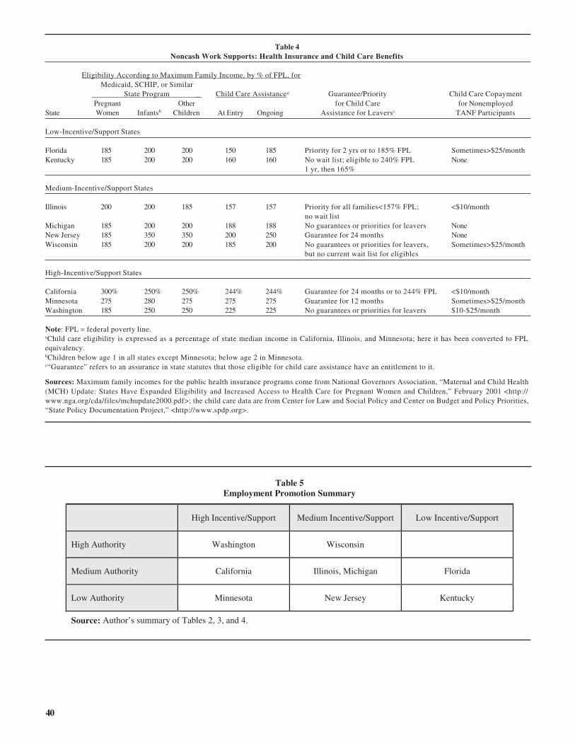
40

Table 4 Noncash Work Supports: Health Insurance and Child Care Benefits

Eligibility According to Maximum Family Income, by % of FPL, for Medicaid, SCHIP, or Similar

State Program _ Child Care Assistancea Guarantee/Priority Child Care Copayment Pregnant Other for Child Care for Nonemployed

State Women Infantsb Children At Entry Ongoing Assistance for Leaversc TANF Participants

Low-Incentive/Support States

Florida 185 200 200 150 185 Priority for 2 yrs or to 185% FPL Sometimes>$25/month Kentucky 185 200 200 160 160 No wait list; eligible to 240% FPL None

1 yr, then 165%

Medium-Incentive/Support States

Illinois 200 200 185 157 157 Priority for all families<157% FPL; <$10/month no wait list

Michigan 185 200 200 188 188 No guarantees or priorities for leavers None New Jersey 185 350 350 200 250 Guarantee for 24 months None Wisconsin 185 200 200 185 200 No guarantees or priorities for leavers, Sometimes>$25/month

but no current wait list for eligibles High-Incentive/Support States

California 300% 250% 250% 244% 244% Guarantee for 24 months or to 244% FPL <$10/month Minnesota 275 280 275 275 275 Guarantee for 12 months Sometimes>$25/month Washington 185 250 250 225 225 No guarantees or priorities for leavers $10-$25/month

Note: FPL = federal poverty line. aChild care eligibility is expressed as a percentage of state median income in California, Illinois, and Minnesota; here it has been converted to FPL equivalency. bChildren below age 1 in all states except Minnesota; below age 2 in Minnesota. c“Guarantee” refers to an assurance in state statutes that those eligible for child care assistance have an entitlement to it.

Sources: Maximum family incomes for the public health insurance programs come from National Governors Association, “Maternal and Child Health (MCH) Update: States Have Expanded Eligibility and Increased Access to Health Care for Pregnant Women and Children,” February 2001 <http:// www.nga.org/cda/files/mchupdate2000.pdf>; the child care data are from Center for Law and Social Policy and Center on Budget and Policy Priorities, “State Policy Documentation Project,” <http://www.spdp.org>.

Table 5 Employment Promotion Summary

High Incentive/Support Medium Incentive/Support Low Incentive/Support

High Authority Washington Wisconsin

Medium Authority California Illinois, Michigan Florida

Low Authority Minnesota New Jersey Kentucky

Source: Author’s summary of Tables 2, 3, and 4.

41

Evaluation of State TANF Programs: An IRP Conference, April 2002

TANF impact evaluation strategies in nine states

review is based on summaries provided on the Research Forum web site (http://www.researchforum.org/) along with the impact analysis methodology paper. In other cases (e.g., Illinois, Kentucky, Michigan, New Jersey, and Washington), the evaluation is in midstream, so that my review is limited to midterm reports.

Consistent with the goals of the Personal Responsibility and Work Opportunity Reconciliation Act (PRWORA), the work-first emphasis of each state’s program is front and center in either the report title or the program title. The evaluations consequently paid much attention to work outcomes or at least job readiness. Table 2 summa-rizes key findings on employment and earnings out-comes—the average employment rates and the average annual earnings for the employed.3 There is remarkable consistency across the states in both employment levels (around 50 percent) and annual earnings (around $10,000–$12,000). Perhaps this is not surprising given the relative homogeneity of the caseload composition across states and the shared economic success in the late 1990s.4

The evaluation criteria

In evaluating the nine state studies, I devote most of my attention to four of the five evaluation criteria established by the National Research Council in their survey of na-tional welfare reform evaluation strategies: these criteria are the populations, outcomes, data, and evaluation meth-ods of interest.5 The panel’s fifth criterion, the questions of interest, is not discussed—not because the questions are unimportant (indeed the number of relevant questions is seemingly limitless), but because all the studies share a focus on two key questions related to labor-market out-comes: What is the impact of program participation on employment and earnings, and what are postwelfare em-ployment rates and earnings?

Populations of interest

There are three prime groups of interest:

Families currently on welfare, because their well-being is potentially affected directly by the welfare policies in place, e.g., work requirements, time limits, sanctions, earnings disregards, and family caps.

Welfare leavers, because their success or failure is an important guide to how current recipients are likely to fare when they in turn leave cash welfare. For example, if leavers have difficulty sustaining employment, or face the prospect of “dead-end” jobs, then policies could be redi-

James P. Ziliak

James P. Ziliak is Professor and Carol Martin Gatton Chair in Microeconomics, University of Kentucky, and an IRP affiliate.

With near unanimity, state governments, granted greater autonomy under the welfare reform legislation of 1996, have constructed their new social assistance programs on a “work first” paradigm.1 Their hope is that these pro-grams can permanently shift the perceptions and behav-iors of current and potential welfare recipients toward work and away from income assistance. The new rules use both stick and carrot: most states have time limits and penalties designed to make cash assistance less attractive, but many also established higher asset limits and earnings disregards that permit households to retain a higher level of earnings and hold greater asset balances without losing benefits.

The U.S. Department of Health and Human Services, states, and private foundations have mounted a strong effort to monitor and evaluate the effects of these changes on the well-being of welfare families and the low-income population in general. The impending reauthorization of Temporary Assistance for Needy Families (TANF) makes this a critical juncture to take stock of what we have learned about the effect of welfare reform on low- income Americans, and of the methods employed to ar-rive at these findings.2

In this article I examine the TANF evaluation strategies adopted by researchers in nine states—California, Florida, Illinois, Kentucky, Michigan, Minnesota, New Jersey, Washington, and Wisconsin. I concentrate on strategies used to monitor and evaluate the effect of pro-gram rules on the well-being of children and families, i.e., impact evaluation, as opposed to strategies used to moni-tor the implementation of new rules and administration, i.e., process evaluation.

In reviewing the state evaluations, I focus on one key report in each state (Table1). These reports differ widely in size, from preliminary summaries of Washington’s Work First program to multiple-volume reports on Minnesota’s Family Investment Plan (MFIP) and Wisconsin’s Child Support Demonstration Evaluation (CSDE). At this writing, the impact analysis of the Cali-fornia evaluation is not yet publicly available, so my

Focus Vol. 22, No. 2, Summer 2002

42

rected toward building the job readiness and human capi-tal of current recipients or toward supports and income supplements for current leavers. The rate at which fami-lies go back onto welfare is also fairly high. If it is possible to identify the sources of such recidivism, pro-grams for current recipients can be redesigned to mitigate cycling on and off welfare.

Low-income families broadly construed include the “working poor,” both single- and two-parent families, and the so-called near poor, i.e., those families not in poverty but who are within, say, 200 percent of the threshold. The near poor face a reasonably high risk of entering welfare, possibly through a major change in fam-ily composition, a prolonged spell of joblessness, or a severe illness.

Within each of the populations are distinct subpopula-tions. Evaluating the well-being of children is particularly critical to any comprehensive research program on the impact of welfare reform. The market opportunities for work, child care, and health may differ by education level and by race. Gender matters: single, female-headed households constitute over 90 percent of the AFDC and now TANF caseload. That said, after passage of PRWORA, most states no longer distinguish between the single-parent and the two-parent caseload, and we might expect the long-term composition of the caseload to shift toward a higher proportion of two-parent families.

Table 3 makes readily apparent that the nine state evalua-tions placed primary emphasis on recipients and leavers. The MFIP, CSDE, and Work First New Jersey studies

Table 1 The Nine State TANF Impact Evaluation Reports, Programs, and Contractors

California: Report: “Welfare Reform in California: Design of the Impact Analysis” http://www.rand.org/publications/MR/MR1266.0/MR1266.0.pdf Program: California Works Opportunity and Responsibility to Kids (CalWORKS) Program Statewide Evaluation Contractor: RAND Corporation

Florida: Report: “Tracking the Outcomes of Welfare Reform in Florida for Three Groups of People” http://www.flawelfarereform.org/reports/documents/CrewTrackingFinalDHHS.pdf Program: Work and Gain Economic Self Sufficiency (WAGES) Program Contractor: Florida State University

Illinois: Report: “Work, Welfare, and Well-Being: An Independent Look at Welfare Reform in Illinois” http://www.jcpr.org/wpfiles/IFStechnicalreport.PDF Program: Illinois Families Study Contractor: University Consortium on Welfare Reform

Kentucky: Report: “From Welfare to Work: Second-Year Panel Study of Families and Children” http://www.researchforum.org/cfm/report.cfm?id=108 Program: Kentucky Transitional Assistance Program (K-TAP) Contractor: University of Louisville

Michigan: Report: “Barriers to the Employment of Welfare Recipients” http://www.ssw.umich.edu/poverty/wesappam.pdf Program: Women’s Employment Study Contractor: Poverty Research and Training Center, University of Michigan

Minnesota: Report: “Reforming Welfare and Rewarding Work: Final Report on the Minnesota Family Investment Program” http://www.mdrc.aa.psiweb.com/Reports2000/MFIP/MFIP-ExSum-Final.htm Program: Minnesota’s Family Investment Program (MFIP) Evaluation Contractor: Manpower Demonstration Research Corporation

New Jersey: Report: “How WFNJ Clients Are Faring Under Welfare Reform” http://www.mathematica-mpr.com/PDFs/wfnj.pdf Program: Work First New Jersey Evaluation Contractor: Mathematica Policy Research, Inc.

Washington: Report: “The Work First Study: 3000 Washington Families” http://www.wa.gov/WORKFIRST/about/StudyDescript.htm Program: Washington Work First Study Contractor: Social and Economic Research Center, Washington State University

Wisconsin: Report: “W-2 Child Support Demonstration Evaluation, Phase I: Final Report” http://www.ssc.wisc.edu/irp/csde/phase1-tocs.htm Program: W-2 Child Support Demonstration Evaluation Contractor: Institute for Research on Poverty, University of Wisconsin-Madison

43

did, however, include new applicants in their populations of interest, permitting the evaluation to look at cohort differences.

Quite absent from the majority of studies is a research focus on low-income populations at large. We do not really know whether the new welfare policies have had a behavioral impact on this broader cross-section of fami-lies, and the nine state evaluations bring us no closer. Because certain policies, such as expanded earnings dis-regards and liquid-assets limits, reach deeper into the income distribution, and because other policies focus on family structure (notably by encouraging two-parent families), an understanding of how the working poor and/ or the near poor are faring under the new rules is highly necessary, yet here it is largely neglected, with minor exceptions in the case of Florida and New Jersey.6

On a more positive note, however, most of the studies examined the comparative effects on important subpopu-lations: one- versus two-parent families, white versus nonwhite household heads, urban versus rural families, and household heads with higher versus lower education. These data provide added flexibility in assessing how

Table 2 Employment and Earnings Results from Nine States

Average Annual Earnings Months Between Average Employment Rates (%) _ for Those Employed ($) _

Initial and Final Initial Final Initial Final State Measurements (Control) (Treatment) (Control) (Treatment)

Florida 21 38 52 11,005a Na

Illinois Na 53 Na 12,588 Na

Kentucky 12 46 58 7,728 10,332

Michigan Na 62 Na Na Na

Minnesota 27 (37)b (50) (9,348) (11,460)

New Jersey Na 50 Na 12,492 Na

Washington 9 39 52 7,380d 10,836

Wisconsin 12 (79/79)c (78/79) (4,272/5,885)e (4,380/6,040)

Note: The table shows employment rates and average earnings at the start of the period as compared to the end of the evaluation period (or, for those studies in progress, the most recent levels), when these are available. Two states use formal experimental designs (Minnesota and Wisconsin), so I record the respective levels for the control and treatment groups in bold; the difference between the two yields the “treatment effect.” Washington uses nonexperimental methods in the earnings model and these are highlighted in italics.

aWeighted average across three groups for evaluation period.

bResults are for single-parent families.

cThe first number for each of the treatment and control groups in Wisconsin refers to 1998, and the second to 1999. The percentages refer to any earnings throughout the year for resident mothers.

dThe Washington nonexperimental estimates are obtained from Figure 3 in M. Klawitter, “Effects of WorkFirst Activities on Employment and Earnings” (2001) (http://www.wa.gov/WORKFIRST/about/studyActiv.pdf). The control (treatment) group estimates refer to those who did not (did) complete pre-employment training activities.

eEarnings are for all resident mothers, not just those employed. For employed resident mothers, average earnings across the treatment and control groups were $5,576 in 1998 and $7,652 in 1999.

Table 3 Populations Studied in Nine State Evaluations

Recipients Leavers Low-Income

California U U

Florida U Ua

Illinois U U

Kentucky U U

Michigan U U

Minnesota Ua

New Jersey Ua U Ub

Washington U U

Wisconsin Ua aThe sample also included new applicants to the program after initial assignment of current recipients.

bAs part of the Community Study aspect of New Jersey’s evaluation, a separate survey was fielded that included households up to 250 per-cent of the poverty line.

44

policy effects may vary, at least within the recipient and leaver populations.

Outcomes of interest

Historically, economists have focused on family income levels as a measure of individual or collective welfare. Part of this narrow focus comes from convenience, be-cause most national surveys of households measure in-come. Part emanates from the development of the Na-tional Income and Product Accounts by Nobel economist Simon Kuznets, which provided a common benchmark to compare living standards within and across countries.

Another Nobel-prize-winning economist, Amartya Sen, eschewed this focus on income as the sole barometer of well-being in favor of multiple indices which more ad-equately capture the “capabilities” of individuals and families to function in an economy. To be sure, income is to be maintained as a measure of welfare in Sen’s view, but so are the direct and indirect costs and benefits of obtaining the income, e.g., access to human capital, job quality, transportation mode to work, health benefits, ac-cess to child care, and the physical and mental health of children and their parents.7 The evaluation of welfare reform, in Sen’s view, must necessarily be broad in scope.

Critical indices of family well-being include:

Education. What types of education and training have the household head(s) and children completed and what addi-tional types do they have access to pursue? Education is strongly positively correlated with income, and nega-tively correlated with crime and alcohol or drug depen-dence; thus avenues to independence often stem from solid human capital formation.

Employment. Is the head working, and if so, how many hours, how many jobs, what types of jobs, and at what time of day (e.g., day or night shift)? If custodial parents are working night shifts, then is adequate child care avail-able?

Income. We would like to know the usual hourly wage, the levels and growth of earnings, the amount and types of public assistance (cash versus in-kind), the extent of in-terfamily transfers, and any child support received.

If possible, there should be a measure of disposable in-come, which is typically defined as the sum of labor and capital income, less taxes, plus transfers and credits. The last is very important, given the increased generosity of the Earned Income Tax Credit (EITC) in recent years. Ideally, researchers would also document “discretionary” income. If low-income households have money left over after the critical expenses (food, shelter, and health care needs, for example) are met, they then have opportunities for social mobility, by moving to a new neighborhood, sending children to better schools, or saving for a down payment on a home.

Health and Family Life. Education, employment, and income are clearly factors in well-being, but other aspects of human “capabilities” are usually considered also: the physical and mental health of the parents and children, the cognitive and social development of children, housing quality, and family structure and relations. For example, are welfare recipients job ready, or do they face physical and/or mental barriers to gainful employment? Does the cognitive development of children formerly on welfare thrive or deteriorate with a working parent? Are parent- parent or parent-child relations of the nurturing type, or are people more prone to destructive behaviors such as physical or mental abuse? Although identifying the causal channels is often a challenge of the first order, there is a clear need for research on these and related issues in order to more comprehensively inform policy.

The nine state evaluations have cast their nets very broadly in terms of outcomes of interest, much closer to the ideal notions of well-being set out by Amartya Sen than to the income-based metrics typically employed by economists. All these reports collected and analyzed data related to education, employment, earnings, welfare use, and the well-being of parents and children. All save Florida sought to collect information on disposable in-come.8 This ambitious evaluation focus conveys a com-mitment on the part of state agencies and evaluators to obtaining a comprehensive view of overall well-being. In general, though, whereas Sen would argue that good health and a stable family life are end goals, most of the nine states view good health and family stability as a means to an end, the end being employment and self- sufficiency.

Data of interest

In the context of welfare evaluations, high-quality datasets are characterized by (1) a large cross-section, so that statistical tests have reasonable power even in analy-ses of narrowly defined subpopulations; (2) a wide array of information to address the outcomes of interest listed above; (3) data that are well measured and not polluted by extensive biases arising from item nonresponse (i.e., missing answers to individual questions) and survey nonresponse (i.e., complete nonparticipation by a sample member); and (4) longitudinal design, so that it is pos-sible to follow families over time.

State-level administrative data offer a fruitful source of information, particularly for welfare recipients and leavers, and tend to satisfy criteria (1), (3), and (4). These data include social benefit programs, but the information they report is often limited in scope and it may be neces-sary to merge several administrative data files to obtain a more complete profile of labor market and public assis-tance activity. Even such an enlarged dataset is likely to lack important demographic information.

Survey data, preferably those that can be linked to admin-istrative data and that follow families over time, are the

45

best way to gain detailed information on the well-being of families.

All nine studies make use of administrative, survey, and longitudinal data as a key part of their analyses. Most often the administrative data are from social benefit pro-grams—TANF, food stamp, and Medicaid caseload data-bases, and Unemployment Insurance records, which con-tain basic wage and employment history data for those in covered employment. The administrative data are then typically linked to survey data, which in all nine evalua-tions are longitudinal, making it possible to collect de-tailed information over time. This approach of combining administrative and survey data over time is likely to be-come a predominant technique in welfare impact evalua-tions.

The studies defined the samples of recipients and leavers differently. For example, a common approach to deter-mining which recipients were eligible for sample inclu-sion was to select families who were TANF recipients in a given month (California, Kentucky, Michigan, New Jer-sey, Washington, Wisconsin) or a calendar quarter (Florida, Illinois). In the MFIP evaluation, cases were randomly assigned over a two-year period, whereas in both New Jersey and Wisconsin new applicants were added to the sample for several months after initial as-signment.

Selection of study samples for welfare evaluation can present a particularly complex set of issues.

First, there are both seasonal and cyclical components to welfare utilization. All else equal, more people are on welfare in winter months than in summer months.9 A sample selected in a given month or quarter may be dif-ferent from a sample selected over, say, six to twelve months, and a wider window for sample inclusion seems important to avoid any bias caused by seasonal variation. In these nine studies, the differential effects of economic cycles seem to be of less concern. Even though the bulk of the samples were drawn near the peak of the 1990s busi-ness cycle—by many accounts very beneficial for low- income families—there appears to be little evidence that those on the caseload in the late 1990s were very different from those on the caseload at similar points in other cycles.10

Second, how did researchers compensate for nonrandom survey samples and survey nonresponse? With the excep-tion of Washington’s Work First study, in which the en-tire state TANF population in March 1999 was eligible for inclusion in the sample, the studies employed some form of stratified random sampling.11 For example, the CSDE study in Wisconsin stratified the sample based on W-2 status (“transitioned W-2” and “new W-2”) and by W-2 tier location (“upper” and “lower”), whereas the KTAP study in Kentucky stratified the sample based on county of residence (focusing on 6 of the over 100 coun-

ties in the state). Within each stratum, however, simple random sampling was employed, though the KTAP study also employed quota sampling, whereby sampling is con-tinued until a desired sample size is attained.12 Most of the time, sample weights were constructed to adjust sta-tistically for differential assignment, though I was unable to find evidence of such weighted adjustment in the KTAP evaluation.

Overall response rates were typically 80–90 percent, though there are some notable exceptions. The Florida WAGES survey had dismal response rates on the order of 18–45 percent, Washington’s Work First Study had re-sponse rates of 55–70 percent, and the noncustodial par-ent survey in Wisconsin’s CSDE study had very low response rates of about 30 percent.

When response rates are better than 80 percent, it is not uncommon for researchers to ignore potential problems of nonresponse bias, though good practice dictates at least a comparison of observable characteristics if a sub-set of data is available for both respondents and nonrespondents. When response rates fall below 80 per-cent, it is possible for analyses to be compromised unless there is some adjustment for nonresponse.

I could find no evidence of such adjustment in the Wash-ington Work First Study. Some adjustment was made in the Florida evaluation, but the method adopted, Bayesian Multiple Imputation, suffers from two significant draw-backs. First, multiple imputation is most often applied to situations of item nonresponse, not survey nonresponse as in the Florida study, especially when upwards of 80 percent of the sample needs to be imputed. Second, the method is valid only if survey participants and nonpartici-pants do not differ in important dimensions, such as wel-fare participation. In Florida, there is evidence that the two groups differed in their use of welfare and the amounts of benefits they received; these circumstances might jeopardize the nonresponse adjustment mecha-nism.

The noncustodial parent portion of the Wisconsin CSDE survey was plagued by the high nonresponse typical of surveys of this hard-to-reach population. As a conse-quence, a formal model of survey participation was esti-mated using administrative and survey data. Weights were constructed based on the inverse (fitted) probability of survey participation, and then adjusted for the strati-fied design in the main sample.13

Evaluation methods of interest

The types of populations, outcomes, and data of interest in impact evaluation research are often directed by the intended method of evaluation. Is there to be a formal experimental design where one subset is randomly as-signed to a “treatment” group, which is subject to a new policy (or policies), and another subset randomly as-

46

signed to a “control” group not subject to the policy? Will a nonexperimental design be employed, whereby regres-sion-based methods are used to compare families affected by the policy to similarly situated families that are not affected by the policy and are not randomly assigned? Or will the primary focus be a descriptive monitoring of outcomes, possibly over time?14

The power of the experimental design emanates from the fact that the correct counterfactual outcome is identified by randomly assigning people to treatment and control groups, thus implicitly ruling out the possibility that par-ticipants will “self-select” into the program on the basis of characteristics observable and unobservable to the evaluators. But experiments can be compromised on many fronts. The initial assignment may not be random, there may be substitution bias (when the control group also receives some form of treatment) or general equilib-rium effects (when behavior overall reacts to the policy change), and subjects may drop out of the experiment.

The nonexperimental approach generally offers the ad-vantage of large sample sizes and detailed questions, improving the power to detect policy effects within key subgroups. The main disadvantage is that identifying the correct counterfactual is at best difficult, and at times impossible.

With respect to welfare reform, descriptive monitoring has been and will continue to be a crucial component of evaluation. Monitoring studies provide detailed informa-tion on the trends in employment, income, welfare utiliza-tion, health, and overall well-being. Although averages and variances are typical statistics reported, for many variables we want to know more about the distribution. For example, reporting the average amount of child sup-port received does not adequately convey the fact that a large percentage of custodial parents receive no support at all from noncustodial parents.

Table 4 Methods Utilized in Nine State Evaluations

Monitoring/ Experimental Nonexperimental Descriptive

California U U

Florida U

Illinois U

Kentucky U

Michigan U

Minnesota U

New Jersey U

Washington U U

Wisconsin U

The importance of choosing the correct evaluation method cannot be overstated. Consider two questions of primary interest to policymakers: what is the impact of TANF on employment rates, and what are the employ-ment rates of those who have left welfare? The outcome of interest is the same for each question, but answering the former requires an impact analysis, whereas the latter simply requires monitoring and thus does not provide the counterfactual to answer the impact question.15

Formal impact analyses are relatively rare among these nine states. In general the studies utilized monitoring methods of evaluation (Table 4). In some cases informa-tion was presented for a single cross-section, but more often than not the studies presented a comparison over time, which permits the identification of simple trends in outcomes of interest such as employment, income, and health. When adjusted for nonrandom sampling and nonresponse error, these descriptive statistics provide a benchmark from which more formal analyses can be con-ducted.

Only the MFIP and CSDE programs conducted random-ized trials, and only the Washington Work First and CalWORKS evaluators used, or plan to use, nonexperimental evaluation methods.16 Both the MFIP and CSDE studies contained thorough and detailed docu-mentation on the implementation of the randomized trial, on the survey design and the construction of weights (especially CSDE), on the outcomes of interest, and on the evaluation methods. For outcomes, MFIP reports the simple mean difference between treatment and control groups as the average treatment effect, whereas CSDE reports regression-adjusted mean differences, the latter adjustment often improving the efficiency of the esti-mated mean differences.

Summary

The nine state TANF impact evaluations tell us a great deal about child and family well-being, the employment and earnings of parents, and transfer-program participa-tion, typically following the same family for two to six years. From MFIP, for example, we learned that the pro-gram policies, at least among single parents, led to higher employment, income, and child well-being, and to lower domestic abuse. From CSDE we learned that if the state passes through to the resident parent all child support received from the nonresident parent, child support re-ceipts among welfare mothers are higher, and a higher percentage of nonresident fathers pay child support, though there appear to be few to no benefits for child well-being. In addition, both the MFIP and CSDE studies conducted cost/benefit analyses, which revealed that there were no net costs to the government for the CSDE pass-through experiment and positive net benefits, on the order of $2,000 per family, in the MFIP experiment.

47

But to date, the research has unquestionably fallen short in the failure to consider possible effects on the broader low- income community and in the scarcity of formal impact analysis. New and modified program rules are on the hori-zon as TANF reauthorization proceeds. States should be preparing now to evaluate the effects of these changes, and as part of that effort, should consider seriously (1) expand-ing the populations of interest from recipients and leavers to the low-income population, to provide greater detail about the impact of welfare reform on vulnerable families; and (2) expanding those evaluations from simple monitoring studies to full-blown studies based on experimental designs, supple-mented with nonexperimental evaluations to permit analyses of large subgroups. Continuing to debate and implement welfare policy without a basis of scientific knowledge could be very costly to the families affected and to local, state, and federal governments. �

1I wish to thank Glen Cain and Jeff Smith for comments on an earlier version of this paper presented at the IRP Conference on State Evalu-ations, April 4–5, 2002.

2See the recent special issue of Focus, Vol 22, no. 1 (2002), for a broad perspective on welfare reform and TANF reauthorization.

3With the exception of Minnesota and Wisconsin (and to a lesser extent Washington) the data presented in Table 2 are not derived from experimental or nonexperimental impact analyses; rather, they are simple summary statistics.

4Wisconsin’s CSDE results differ from the other studies in that em-ployment rates are for those “ever employed” rather than currently employed, and earnings averages are for all sample members, includ-ing nonworkers. The primary focus of the CSDE is on the effect of the child-support pass-through on child support receipts and payments, not necessarily on employment.

5National Research Council, Evaluating Welfare Reform in an Era of Transition, Panel on Data and Methods for Measuring the Effects of Changes in Social Welfare Programs, ed. Robert A. Moffitt and Michele Ver Ploeg (Washington, DC: National Academy Press, 2001).

6One of the three groups included in Florida’s evaluation consisted of Medicaid families who were income-eligible nonparticipants in cash assistance. The Florida report does not reach the near poor per se, but it touches upon an important behavior—nonparticipation by those who are in fact eligible. The New Jersey evaluation has three compo-nents, a Client Study, a Community Study, and a Program Study. Within the Community Study, which is a case study of Newark, Camden, and Cumberland County, the population of interest expands to families within 250 percent of the poverty line. But this portion of the study is still somewhat of a sideshow compared to the main focus on recipients and leavers.

7A. Sen, The Standard of Living: The Tanner Lectures (Cambridge: Cambridge University Press, 1987).

8Here defined as labor and nonlabor income, plus transfers, minus taxes, plus the EITC.

9J. Ziliak, D. Figlio, E. Davis, and L. Connolly, “Accounting for the Decline in AFDC Caseloads: Welfare Reform or the Economy?” Jour-nal of Human Resources 35, no. 3 (2000): 570–86.

10See R. Moffitt and D. Stevens, “Changing Caseloads: Macro Influ-ences and Micro Composition,” unpublished paper, Johns Hopkins University, 2001.

11The Michigan study used simple random sampling, but only one county was selected as the relevant population. To the extent that this

county is representative of the state TANF population, then inferences can be drawn for the state as a whole; however, this is highly unlikely, so that inferences must be restricted to that county unless some later adjustment is made to account for the relative share of TANF cases in the county.

12See A. Deaton, Analysis of Household Surveys (Baltimore: Johns Hopkins University Press, 1997) for a recent discussion of survey sampling and the econometric issues surrounding sample weights.

13The techniques are fully described in J. Ziliak and M. Krecker, “Nonresponse in the Survey of Wisconsin Works Families,” W-2 Child Support Demonstration Evaluation, Vol. III, Technical Report 6, Institute for Research on Poverty, University of Wisconsin-Madi-son, 2001.

14There is a vast literature on the strengths and weaknesses of alterna-tive impact evaluation methods For detailed reviews see, among oth-ers, R. Blundell and M. Costa-Dias, “Evaluation Methods for Non- Experimental Data,” Fiscal Studies 21, no. 4 (2000):427–68; J. Heckman, R. LaLonde, and J. Smith, “The Economics and Economet-rics of Active Labor Market Policies,” in Handbook of Labor Eco-nomics 3A, ed. O. Ashenfelter and D. Card (Amsterdam: North Hol-land, 1999), pp. 1865–2097; C. Manski and I. Garfinkel, Evaluating Welfare and Training Programs (Cambridge, MA: Harvard Univer-sity Press, 1992); National Research Council, Evaluating Welfare Reform in an Era of Transition; J. Wooldridge, Econometric Analysis of Cross Section and Panel Data (Cambridge, MA: MIT Press, 2002), pp. 603–44.

15I thank Jeff Smith for stressing this point in an earlier draft.

16A nonexperimental component of the CSDE evaluation was released after I completed this review: D. Meyer and M. Cancian, eds., W-2 Child Support Demonstration: Report on Nonexperimental Analyses, Institute for Research on Poverty, University of Wisconsin-Madison, 2002.

48

Evaluation of State TANF Programs: An IRP Conference, April 2002

Perspectives of researchers and federal officials: A panel session

Bruce Meyer, Northwestern University: I would like to emphasize some of the same things that Jim Ziliak em-phasized in his talk. A few of them I would like to push even farther, because I think they’re important. First of all, we were asked to answer what we need to learn; we need to learn what policies work and how well-being changes, how much policies cost. Jim emphasized that we should look at a variety of measures of well-being and I would like to add to the list or emphasize more things like child test scores, behavior at school, fertility, and mar-riage. Also Jim emphasized looking at disposable in-come; I think we should go one step further and look at measures of consumption or material hardships, like dif-ficulty paying for rent or going to bed without having eaten enough. If one looks at the work in detailed inter-views by, say, Kathryn Edin and Laura Lein and others, they’ve argued that income doesn’t do a good job of measuring the well-being of people at the bottom and I’d like to push people to look more at consumption.1 The reason is that there is a lot of underreporting of income, particularly at the bottom (food stamps, TANF, EITC, housing subsidies, and the like). For example, if you look at the tenth, twentieth, thirtieth percentile of consumption of low-educated single mothers, it is twice their reported income. Consumption measures, whether you are asking about food, housing, or about hardships like difficulty paying rent or having enough food, are more direct mea-sures of well-being.

I think the National Research Council reports did an excellent job of summarizing the benefits and problems with different approaches and I would like to even push further Jim’s preference for random-assignment evalua-tions and to a lesser extent quasi-experimental evalua-tions over the monitoring approaches. The problem with monitoring is we just can’t, in general, estimate the causal effect of the policy. We can’t figure out if a different policy improves things and to what extent. There is typi-cally no comparison group or counterfactual to know what would have happened in the absence of the policy. We generally don’t look at the full populations at risk, including people diverted or discouraged from applying; we maybe just look at people on the rolls and leavers. So we should emphasize experimental evaluations, bearing in mind the caveat in Jim Ziliak’s paper, and including a key acknowledgment that we could only look at those in the system, those who are on the rolls or who have showed up in welfare offices.

Panel Chair: Robert Haveman, University of Wiscon-sin–Madison

Participants: Jonah Gelbach, University of Maryland, Karl Koerper, Administration for Children and Families (ACF) in the Department of Health and Human Services, Bruce Meyer, Northwestern University, Don Oellerich, Office of the Assistant Secretary for Planning and Evalu-ation (ASPE) in the Department of Health and Human Services, Wendell Primus, Center on Budget and Policy Priorities (CBPP), and Jeff Smith, University of Mary-land.

Robert Haveman, University of Wisconsin–Madison: Obviously the purpose of evaluation studies is to give advice to policymakers. One of the important questions that has been thrown out at this conference is the follow-ing: If we in state government were to have a million extra dollars available, how do we allocate it to get the biggest impact in terms of our objectives?

It’s that sort of question that evaluation studies should be designed to answer. In the current context, if we need to encourage work participation rates, what strategies are available that would be most effective in attaining that goal? Jim Ziliak has given us, in some sense, a counsel of perfection for evaluating welfare reform and alternative welfare reform strategies—call it the Ziliak critique. Nearly everything that we would now say would have to be held up to the high standards that critique requires. Jim wants more formal evaluation, meaning random assign-ment, less informal assessment, less monitoring. He would like more focus on the entire low-income popula-tion, which probably means less focus on leavers and recipients.

So the question which follows directly from Jim’s paper is “How should we in the research community and at the state level proceed?” How can we improve the evalua-tion-type information that we are going to be providing policymakers? Do people have ideas for how the aca-demic community and state governments can better meet the Ziliak critique? What are the constraints on states in improving the quality of research and evaluations of wel-fare reform? Are they financial resources? Are they staff resources? Are there too few staff interested in evalua-tion, or are the interests of the staff in other areas? If we can identify those constraints, are there options for relax-ing them?

Focus Vol. 22, No. 2, Summer 2002

49

Now as for nonexperimental evaluations, quasiexperi- ments with difference-in-difference types of experiments, it is much harder to make general statements, because those experiments, those methodologies differ a lot de-pending on circumstances. But one general comment is that it’s important that you have a good comparison group. When you’re looking at outcomes for one group you need to have a group that you think is comparable in some way. There are a lot of ways to assess comparability and to see if the comparison group has responded simi-larly to other things going on in the state over time. So I will leave it at that: a stronger push for more experiments over just monitoring studies and a push to look at more outcomes, including consumption.

Karl Koerper, ACF: As an ACF representative, I of course have to push for experimental design studies as well, and I want to go back and look a little at some of the history of our experience with that, particularly some experience in Illinois. One of the early attempts we made when we were still in the AFDC program to look at employment retention was a project called the Post Em-ployment Services Demonstration. It would prove quite successful because basically people who left employ-ment, stayed employed. I think we got about 80 percent employment among both controls and experimentals.

Illinois was just one of the participants in that study. Had they done the study in the fashion that they wanted, they’d have been doing monitoring studies, just to see if they were doing a good job, and they might to this day be spending the extra money that they were putting into more extensive case management to help people stay employed. But the unit back then was basically sinking good money to get no extra effect, and they abandoned that project after we found that it just didn’t give them any more for their costs. Now they’re involved in the Employment Retention and Advancement Study, in which we basically have 9 states participating in 16 different interventions to test various strategies that build upon what we’ve learned from the Post Employment Services Demonstration. We will again see that some things will work and some things won’t work, but we will know when we’re done whether putting our money toward each strat-egy will work and what we get for our dollar. So when states make decisions about what policies they want to pursue in shrinking budget times, they’ll know whether a particular policy works.

Shrinking budgets actually give you opportunities to use random-assignment evaluation. Illinois once again is a great example. The state was also participating in our Welfare-to-Work rural strategies evaluation. They had a project that helped people in low-income families find work in the rural areas of Illinois and that was threatened with budget cuts—actually was going to be completely eliminated—except that by having the opportunity to join our national evaluation they were able to save it. They were able to cut it back and by denying services to a

control group, because they couldn’t serve everybody, were able to allow it to continue to be funded for a number of years, basically hoping that once we have the results they will be able to go back in front of the legisla-ture and see whether they can defend the program. So if you have some projects going on out there, some inter-ventions that face derailment because of the budget cut-backs, this may be a way to say to the legislature, “Well maybe we can test this. Right now we don’t do random- assignment experiments because taking services away from somebody brings up an ethical consideration. But if we can’t give it to everybody anyway, the situation lends itself to the environment for random-assignment experi-ment.”

Jonah Gelbach, University of Maryland: I like the ran-domized experiment as much as the next guy, and in a world of essentially infinite budgets I can see why you’d want to, in fact, I know why you would want to randomize absolutely everything about the budget set and about the time limit policy and so on, and we’d learn all sorts of wonderful things about every detail of welfare policies. But we don’t seem to have infinite budgets for these things. As a very, very casual consumer of the state evalu-ations—I certainly haven’t come close to the Ziliak per-formance of having read nine major reports—what I find interesting partly is that a lot of these evaluations look at different populations and it’s hard to compare those populations across states. The state policies which we are evaluating are frequently or almost always multidimen-sional in ways that make it less than obvious how to interpret the treatment effect and so I wonder if the ex-pense is really entirely justified.

I know that I’m taking a somewhat unpopular position, but it’s one that has a relatively venerable history in this debate over experimental versus nonexperimental policy research design. I wonder whether it would be better to spend a good chunk of money on designing administra-tive data systems that would be up and, if not available for public use, at least relatively easy for researchers to ac-cess. In a sense, academics are a very cheap source of labor. There are a lot of dissertations that need to be written because there are students, and there are a lot of papers that need to be written because there’s tenure to be gotten. I am only slightly kidding, because making good administrative data, particularly panel data, available would provide the impetus for a lot of research to be done on the kinds of evaluations that the public or policymakers would like to see.

We teach our students how to do nonexperimental re-search on these sorts of policies and I know, at least with respect to the UC Data system and some of the data have been put up regarding California caseloads, that several very high quality papers have been written that have really expanded our knowledge about things like the im-pact of local labor market conditions on transitions into and out of welfare and those sorts of questions. Had those

50

data never been put up and instead that money spent on randomized designs to test the impact of one thing on another, some of those papers might never have come out.

I think there’s a trade-off between the long-run investment in these sorts of resources and very unquestionable identifica-tions from experimental designs, in which the program evaluation has to stop at some point because the evaluators have spent all the money and now it’s time to go home. I’d like to argue for some balance in how our resources are spent. I think the last thing we need to worry about is the labor to actually implement some of these evaluations. What we do need to worry about is providing the data.

With respect to the experimental designs that are done, I think it’s important that somebody keep track of the iden-tifying numbers, like social security numbers, because being able to look at the long-run impacts of some of these programs 5 or 10 years from now or maybe longer than that would be very valuable.

On a relatively unrelated point, I wanted to express the concern that I don’t really feel that I know much about the extent to which participants, and especially potential par-ticipants, understand the rules of the programs. I am told that in one state evaluation of the old AFDC plan versus its newer plan, apparently 70 percent of both treatment and control groups thought that they were subject to time limits. Maybe I misunderstood, but that’s a horrifying thing if you are trying to understand whether time limits have any impact on people. If people don’t know that there are time limits, then the limits probably don’t have any impact until the last minute, and then it’s maybe a little too late. I think it’s great that they ran the survey and asked people. More research on that front would be tre-mendously valuable for those of us who do academic research, because frequently we just have to take it at face value that people know the incentives they face.

The very last thing I’ll say is that one of the problems with randomized designs is that they tend to be either stock-sampled or flow-sampled, which is to say that they sample either people who are already on the program when the reform kicks in or people who want to enter the program after the reform has started. That’s a wonderful way to know about the people who either are on the program or want to get on it. But it’s not such a great way to know about the people who could plausibly have wound up on the program, particularly in a time when we know that the economy changed mightily. We may be missing a lot of the population in trying to evaluate what’s happening. I don’t know what the answer is, but not having any sense of potential entry effects is arguably damaging.

Haveman: I am going to exercise the prerogative of the chair and make a couple of comments now. It seems to me that Jonah put his finger on one of the critiques of Jim

Ziliak’s paper and I would like to emphasize it. The paper sets a very high standard and then simply asks what we can do to move more closely toward that standard without ever mentioning the cost of doing so. At the margin, if you have another million dollars to be spent on studying the effects of welfare reform, do you learn more by, let’s say, sponsoring a randomized experiment of some limited intervention, or in fact would we all be benefitted by allocating that money to continuing and improving the monitoring, leavers-type studies? I think that’s an open question and I don’t think Jim’s paper has addressed it. Maybe one question that would focus exactly on the issue would be to ask yourselves, “Have we in fact learned more from very costly, extensive, randomized experimen-tal designs in studies such as the one of MFIP or the CSDE study here in Wisconsin than we have from the much less costly monitoring studies of leavers that have been done in the states?”

Jeff Smith, University of Maryland: I think my remarks will be a little closer to what Jonah said. But let me first distinguish here between the questions of interest and the methods we should use, given we have decided on the questions of interest. I think those two things have gotten a little confused in the discussion about random assign-ment. If the question is, “What happens to people who fall off of welfare because of time limits?” we don’t need to do any experiments to answer that question; monitoring studies will do just fine. If our question is “What’s the impact of this treatment for these people versus that treat-ment for these people?” then we want to do an experiment if we can, because that’s going to give us the most cred-ible answer in most circumstances.

I expected to come to this conference and learn something about welfare evaluations, and what I have learned is that we haven’t learned much about welfare evaluations yet. But I have learned a lot about what the government people think about these issues and that’s actually really interesting. One thing that I’ve heard people saying is that research is a public good (they don’t mean it, of course, but that’s what they have been saying). So if you say to the states, “do experiments, do experiments, do experi-ments,” what you are basically saying to them in general is “Please provide an unacknowledged good to all the other states. It will be useful to you too but it will mainly be useful to everybody else.”

That’s quite a request to the states and I can see why they are not eager to do that. They have their own questions, that to some extent can’t be answered by random assign-ment because they are questions that the states want an-swered tomorrow. Some of those questions could be an-swered by reading the literature, so I won’t let the state people off the hook entirely. But it seems to me that maybe there’s a division of labor here—in fact, in some ways the only economic justification for federal involve-ment in this area might be as a knowledge producer.

51

We learned a lot from the MDRC work-welfare experi-ments over the ’80s and during the early ’90s. We don’t need to do any more of those—that’s a great example of an experiment that now would be a waste of money be-cause we know how well job search works for this popu-lation. But it generated a good deal of knowledge. The individual states did the experiments and then we changed some national policies for all states on the basis on the knowledge provided by a few states. That’s some-thing the feds arguably ought to be paying for. A question that would be relevant to TANF would be, “How do recipients respond to different types of sanctions?” That’s information that would be useful to every state— almost every state that we’ve heard about here has some sort of sanction regime. My impression is that policymakers ought to know what happens if you take away 10, 15, or 20 percent? The whole point of the program is income maintenance—or at least part of it is income maintenance—and to punish by taking away in-come is shooting yourself in the foot. Maybe we ought to consider other sanctions: treatments like time taxes, lei-sure taxes, as we do to people now in some states when they have automobile tickets; we give them a choice between paying cash or wasting some of their time at court or in driving school. This sort of thing is ideal for an experiment, this is a public good that can benefit all the states. So, pitch number one is, let’s do some experiments that provide public goods in terms of useful knowledge to the states.

Point two is data. This is echoing Jonah—if you give them the data they will come. You can get a lot of free research done just by making interesting data available. I was shocked that it sounds as if some of the states don’t actually know, can’t tell you, what services are applied to whom, in the population. They can’t tell you who was sanctioned, they can’t tell you how many were sanc-tioned, they can’t tell you why they were sanctioned, they can’t tell you how many people got this service or that service. Everybody’s got to know that. To me that’s basic fiduciary duty to the taxpayer, although I don’t mean to sound sanctimonious here. Not only that but it’s useful to the state in figuring out what they’re doing and knowing whether they’re providing services equitably.

So better data in this case are useful to states but would also be useful to researchers, first of all because of mea-surement error. On the Urban Institute site you can see policy variables—this state does this, this state does that—but you don’t know what happens. That’s what they say, but one state may actually sanction 1 percent and another may sanction 10 percent. You’d like to know that, so that you can take account of that when you’re doing a study matching this information on state policies to some sort of larger national dataset.

I think it would be useful to do some general method-ological research on how well we can measure participa-tion in TANF. Do we know whether we are any better at

doing it than under AFDC, where the programs were the same in every state? We know that AFDC was underesti-mated, maybe TANF is underestimated; maybe it varies across states. Some of our research will use these national surveys; there’s no way around it. How well do we mea-sure services received and sanction impositions in these surveys? Do people know that they’ve been sanctioned? Do they know when they’ve gotten a service? Some work I’ve done suggests that people often don’t know.

It’s apparent that some states have developed really good models for making administrative data available to the research community and other states haven’t. A really useful activity that some institutions, maybe even IRP, could undertake would be to describe such models and then disseminate that information to the other states so that they could then try to emulate those successful mod-els of making administrative data available to research-ers.

One last point: yesterday we were discussing perfor-mance standards and we heard statements like “We don’t use the performance standards for evaluations, we just use them to manage the program.” I don’t know what that means. We can poke a little farther and you get the im-pression that people don’t call it evaluation but really it’s evaluation. The performance measures are actually lev-els, there’s no counterfactual here, but people are speak-ing as if they were impacts. They’re not, they’re levels. There is some literature on this; it suggests that the corre-lation between the outcome levels and the impact, the net gain, the actual difference the program is making, is pretty small and maybe it’s zero.

That’s a problem, and I think we need to do two things about that. First we need to keep repeating over and over again, “These are not impacts, these are levels.” It doesn’t mean you don’t want to know them, it just means you have to interpret them correctly, and maybe you don’t want to attach high-power rewards to these things until we’re a little bit more sure that they are actually related to impact. The second thing is that we want to do some research to find performance measures. We need some-thing that can be calculated quickly and inexpensively, but maybe there is something that can be calculated quickly and inexpensively that is also correlated with impact. We don’t know that, but we do know that what we are using now doesn’t give us that.

We ought also think a little bit about alternative manage-ment tools besides outcome levels and performance stan-dards. There is a whole literature on this in public manage-ment; there are, for example, input-based performance measures and some states already have those.

Wendell Primus, CBPP: I really want to emphasize that in my view we’ve probably done too many welfare leaver studies and now we need studies of low-income popula-tions. TANF right now is only covering, when you look at

52

parents with children, probably about 1.7 million. That is a small fraction of the low-income households, no matter how you define them. We need to understand better which fraction of those low-income households find their way on to TANF and exit TANF to really understand what is going on.

The second, and the big story, in some sense, of TANF, is that we’ve reduced cash expenditures by probably on the order of 10–12 million dollars annually and we’ve in-creased child care expenditures also by a large amount. But I don’t think anyone can tell me if we’ve increased child care expenditures by more than the work effort of never-married mothers and if so, by how much. In other words, how much of the TANF cash savings really were moved on to the working poor? And now, in an era of budget cuts, how much are we going to reduce those child care expenditures on the working poor? I don’t think we’ve done nearly enough on that.

The third thing is that an amazing amount of research has been done on the TANF program. There are other income maintenance programs as well. We spend a lot more cash on the Unemployment Insurance Program. I’d like to see some side benefits from all this welfare research. For example, what percentage of the low-income working population is covered by UI in each state? As we have gone through this recession, the question has been: If we really believe in a work-based safety net, how many of those former welfare recipients who lost their jobs, found themselves onto the UI system? Were they eligible or weren’t they eligible, and if not, did they make it over to the welfare system? In some cases, if they were working 25–30 hours, they really should have found themselves onto both systems. Their UI check probably should have been supplemented by a TANF check as well.

The last thing is that there’s some interesting work to be done regarding the male welfare client. There’s an inter-esting paper by Paul Offner and Harry Holzer on the Brookings web site that points out what we’ve done about employment over the last several years for females, as opposed to males—I’m primarily talking now about black males between 16 and 24—sorting out why the perfor-mance of these two groups varies over the same period.2 I challenge the labor economists and others in this audi-ence to help us understand better what is to be done if we really want to increase the employment of noncustodial parents.

Don Oellerich, ASPE: I think it’s important to make the point again that Jeff made: that it’s really the questions that the states have that drive the research, not the other way round. States need very quick answers that are really monitoring answers. They need to know something right away, not 5 years from now or 10 years from now, and the method has to be able to do that. We have to work on those methods to improve the answers because I think a

quick answer is sometimes not right in the long run and people are making bad choices on the information they have in hand.

On the question of the population of interest, I have some thoughts, as one of the people who designed the leavers studies. People thought we were only interested in leavers. They asked, Why aren’t you interested in the caseload? Well, we went from the leavers to the diverters and now we’re dealing with caseload. We’re interested in people who don’t come on to programs, so we’re inter-ested in the whole low-income population. As Wendell Primus pointed out, the cash assistance program touches very few single-parent families relative to the size of the population. Whenever we talk about doing experiments, we’re generally dealing with cash assistance, the cash assistance caseload. Yet about half of the 24 billion dol-lars that states are spending now is not going to cash assistance but to services. We need to know a lot more. Where is that money going? How effectively is it being used?

States and federal officials have a number of important questions that need to be looked at in the next round of research. We’re a long way from doing experiments on child-only cases, but we need to know who are the child- only cases, what are their service needs, and what are the goals for those cases. Are we interested in parents in those families, or only interested in the needs of the children? Those questions have not been addressed in any way and yet child-only cases are a growing proportion of the caseload, about 35 percent.

I think we could do some more experimentation concern-ing the optimal use of case management. One of the things that I am interested in—I have a background in child welfare—is the worker/client relationship and how that affects the outcome for that particular case. Not just the services provided but also the relationship that the worker and the client are able to develop over time may be the telling factor, as it is in child welfare.

We have to have a better understanding of our caseload, which is much more dynamic than it ever was before. We used to say: About half the caseload leaves every year, about half of that caseload goes to work, and 70 percent return within two years—we had this whole welfare dy-namic straight. But now, states are dealing with very different caseloads. Where 4 percent of their caseload was entering every month, on average now it is 10 per-cent; in some states, a third of the caseload comes in every month. The caseload is a revolving door, it’s very dynamic, more like the emergency room than the hospital proper because we’re seeing the critical care group. This makes demands on workers that weren’t there before and we need to learn a lot more through observational studies, through qualitative studies, and through some experi-ments about how we can best be effective.

53

Finally, I’m a strong proponent of random assignment; I think it has its place. The Department is sponsoring earn-ing advancement and retention random-assignment ex-periments on services for the hard to employ.

A selection of comments from the floor

Rachel Hickson, Evaluation Projects Manager, New Jersey Department of Human Services. New Jersey did have some bad experiences with experimental design. I think that drove the state heavily in a monitoring-type direction. Monitoring is the primary focus of our current evaluation, mainly because of the need for very rapid information, especially for public management but also for legislators and for taxpayers; at certain times of the year they get curious about what’s happening in the wel-fare program. In the type of study that we have, with a group of families being followed over time with a peri-odic survey, we’ve been able to make very rapid and frequent changes—enhancements to the program—that we were not able to do in the past, when we had an experimental design and the state was trying to leave the program undisturbed so that that they could get good evaluations.

Koerper: I’m hoping that states are not hung up with past experience with random assignment. Experience with AFDC, which was not a block-granted program, was dif-ferent, probably because TANF is a block grant program with greater flexibility. For one thing, I think a lot of states pursued the waivers more as an opportunity to change their policy than an opportunity for evaluation and as the provider of the waivers HHS was bound by the requirements of 1115 and also bound by the requirement that those waivers be cost neutral.3 So if you wanted to go statewide you had to be cost neutral and you had to have a statewide nonexperimental treatment group and all the rest.

Larry Mead, New York University: One of the attitudes one often hears from evaluators and academics is that unless we evaluate we don’t know whether it works or not. The impression that I’ve had, talking to the actual officials who are operating the welfare system or closely related agencies, is that they often do know what works and they know it without evaluation. Generally speaking, people I’ve interviewed knew what would make their programs work better, they just didn’t have the authority to do it, or they didn’t have the funds to do it. But they knew what worked.

The people who know are the operators, who are close to the program. They have a feel for what’s effective and what isn’t without evaluation. This gets to Jeff Smith’s point, that really evaluation is a public good. You gener-ate findings for people who are further away from the firing line and who don’t have the feel for what works and

who need evaluations—Washington particularly. That’s why evaluation may be most useful at that level or maybe at the state capitol. At the local level, they all have a much better sense of what’s effective. Now maybe when you get down to more fine-grained questions, let’s say the use of case managers, local people won’t have a clearcut opin-ion and there you do need an experiment in order to be sure. But that’s also a situation in which you probably don’t have to have an unserved control group. You can do comparative studies and different treatments and find out what’s most effective, and that’s all you need to do. So actually experimentation, it seems to me—evaluation in general—has a lesser role in improving programs that we sometimes think. It’s really a service to ourselves, people who don’t have this hands-on contact.

Meyer: Let me say a couple of words on Larry’s point. I think the problem with just relying on administrators to use their best guess about what works is that administra-tors think all their programs work. When you look at many of the successful programs that have been carefully evaluated using random assignment they often have a 3 percent increase in employment, or a 5 percent increase in employment. It’s hard to see that that an administrator’s going pick that out without a very careful evaluation.

Mike Wiseman, George Washington University: One problem with Jim Ziliak’s paper—in general it was very informative—was the specific assertion that to inform policy we needed random assignment. This is problem-atic. All the techniques that we’ve found can inform policy. The notion was—and Bruce picked up the no-tion—that what monitoring lacked was a counterfactual. In the many good monitoring studies I’ve looked at, the counterfactuals, it’s very clear, are not counterfactuals, they are sort of a point of reference. You have a notion that something is going on and the monitoring study at-tempts to establish whether or not it is. If there’s a differ-ence between what is going on and what we nominally believe is going on then that is a useful bit of information.

The study Jonah Gelbach mentioned was a monitoring study; the fact that 70 percent of the people didn’t know about the time limit—that’s a monitoring outcome. That tells us something. We can’t deny that that’s informative, so we have to ask what it is that makes monitoring studies pertinent to inform policies.

I want to follow up on something Jeff Smith said, that we know how to do monitoring just fine. We don’t know how to do monitoring just fine, I’d say, and so there really seems to be a need—just as we do conferences on im-proving random assignment—for conferences on improv-ing our procedures for nonexperimental evaluation. At some point it would be very good to have some confer-ences on the way in which we improve the utility of monitoring for feeding into the deliberations over TANF.

54

Joe Hotz, UCLA: In these efforts to get data, one of the key problems is that the kind of information you need for different groups in the low-income population, especially when you start thinking about states, is really difficult to come by. It’s easy to pull out administrative data on participants that we have in the system. I think we could spend a lot more attention on creative ways to get infor-mation on the low-income population. One, which isn’t going to work for everybody, is to start linking together data—survey data, administrative data. There are efforts in California and other states to do that. But also it’s important to support data efforts like the American Com-munity Survey, in which the sample size is large enough to be able to do the analysis within states.4 If you start working on these methods and strategies for dealing with administrative data and these surveys we’ll start to put ourselves in a better position to monitor this low-income population. �

1See, for example, K. Edin and L. Lein, Making Ends Meet: How Single Mothers Survive Welfare and Low-wage Work (New York: Russell Sage Foundation, 1997).

2P. Offner and H. Holzer, Left Behind in the Labor Market: Recent Employment Trends Among Young Black Men, April 2002. < http:// www.brookings.org/dybdocroot/es/urban/publications/ offnerholzer.pdf >.

3From the early 1960s, the Secretary of the Department of Health and Human Services and its predecessors had the authority to waive por-tions of the Social Security Act to permit states to innovate within the AFDC program. These were known as Section 1115 waivers and were not much used until the late 1980s. On waivers, see E. Boehnen and T. Corbett, “Welfare Waivers: Some Salient Trends,” Focus 18, no. 1 (special issue 1996): 5–8.

4The American Community Survey is a mail survey that the Census Bureau plans will replace the long form in the 2010 Census. It will provide estimates of demographic, housing, social, and economic characteristics every year for all states, as well as for all cities, coun-ties, metropolitan areas, and population groups of 65,000 people or more. The ACS is already implemented in selected communities, and it is proposed to begin full implementation in 2003 in every county of the United States. See <http://www.census.gov/acs/www/About/ index.htm>.

55 Focus Vol. 22, No. 2, Summer 2002

New IRP Special Report

Patterns of Long-Term Utilization of Medicaid and Food Stamps by Wisconsin Welfare Leavers

Robert Haveman, Thomas Kaplan, and Barbara Wolfe, with Sandra Barone

Subsidized medical insurance and food purchases through the Medicaid and Food Stamp programs poten-tially improve the health and economic well-being of low- income people, but only if eligible participants receive program benefits. Reports of low rates of take-up and declines in Food Stamp and Medicaid participation fol-lowing passage of welfare reform legislation in 1996 raise concern about the health care and nutritional status of low-income families, particularly those formerly re-ceiving cash welfare. This new IRP report (Special Re-port 82, published July 2002) describes the long-term utilization of food stamps and Medicaid by welfare re-cipients who left the cash benefit rolls in Wisconsin in 1995 (under an early welfare reform regime) and in 1997, after the institution of the Wisconsin Works (W-2) re-forms.

Some key findings of this new IRP report are:

1. Those who left the Wisconsin cash assistance rolls in 1997 were much more likely to take up food stamps and Medicaid than were those who left in 1995.

2. Rates of program take-up reported for Wisconsin are higher than rates reported in most studies of other juris-dictions, even among those who left in 1995.

• One year after exit, mean food stamp take-up rates were 38 percent for the 1995 leavers and 59 percent for the 1997 leavers, compared to rates of 35 percent in most other studies summarized in the report.

• Estimated Medicaid coverage rates in the fourth quar-ter after leaving were 48 percent for the 1995 leavers and 63 percent for the 1997 leavers, compared to a rate of about 40 percent in other summarized studies.

• For children, Medicaid coverage rates in the fourth quarter after leaving are 62 percent for the 1995 leavers and 82 percent for the 1997 leavers, compared

to rates in the 50–60 percent range in other summa-rized studies.

3. Eligibility for food stamps declined with the passage of time after leaving cash welfare, presumably reflecting increased earnings and other income over time, but par-ticipation rates among those who were eligible declined much more quickly. Food stamp eligibility levels among those who left in 1995 declined from 96 percent in the first year after leaving to 82 percent in the fourth year. Participation rates among those who were eligible de-clined from 60 percent at some time in the first year after leaving to 37 percent at some time in the fourth year.

4. Participation rates also dropped among those eligible for Medicaid. Among eligible 1995 leavers, participation rates for mothers dropped from 73 percent at some time in the first year after leaving to 37 percent in the fourth year, and rates for children dropped from 81 percent at some time in the first year to 55 percent in the fourth year.

5. In a sample of children whose mothers had at some time participated in Wisconsin’s W-2 program, those most likely to be uninsured (without either Medicaid or private health insurance) were (a) children who moved at some point during the year and (b) children whose moth-ers worked for firms that offered health insurance (an unexpected result).

6. The introduction of Wisconsin’s BadgerCare program in July 1999 increased eligibility for public health insur-ance coverage (more so among mothers than among chil-dren), but take-up rates among eligible leavers remained approximately constant after the start of BadgerCare.

On the IRP World Wide Web site: http://www.ssc.wisc.edu/irp/sr/sr82.pdf

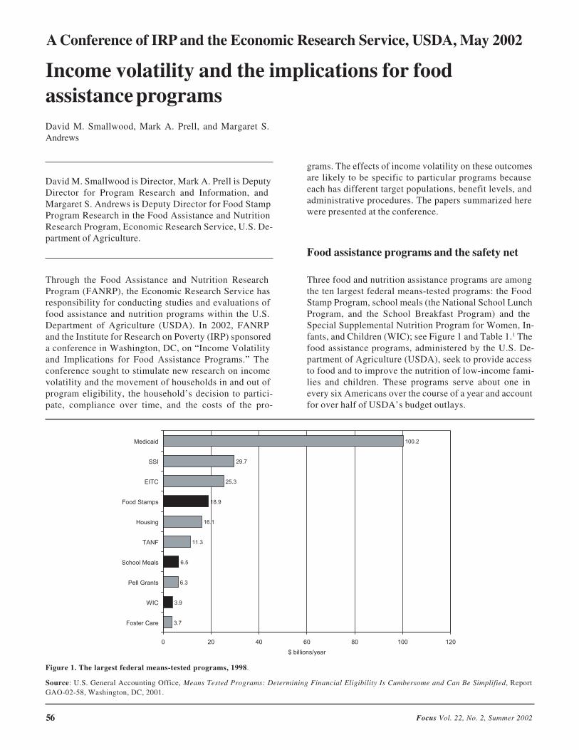
56

Income volatility and the implications for food assistance programs

grams. The effects of income volatility on these outcomes are likely to be specific to particular programs because each has different target populations, benefit levels, and administrative procedures. The papers summarized here were presented at the conference.

Food assistance programs and the safety net

Three food and nutrition assistance programs are among the ten largest federal means-tested programs: the Food Stamp Program, school meals (the National School Lunch Program, and the School Breakfast Program) and the Special Supplemental Nutrition Program for Women, In-fants, and Children (WIC); see Figure 1 and Table 1.1 The food assistance programs, administered by the U.S. De-partment of Agriculture (USDA), seek to provide access to food and to improve the nutrition of low-income fami-lies and children. These programs serve about one in every six Americans over the course of a year and account for over half of USDA’s budget outlays.

David M. Smallwood, Mark A. Prell, and Margaret S. Andrews

David M. Smallwood is Director, Mark A. Prell is Deputy Director for Program Research and Information, and Margaret S. Andrews is Deputy Director for Food Stamp Program Research in the Food Assistance and Nutrition Research Program, Economic Research Service, U.S. De-partment of Agriculture.

Through the Food Assistance and Nutrition Research Program (FANRP), the Economic Research Service has responsibility for conducting studies and evaluations of food assistance and nutrition programs within the U.S. Department of Agriculture (USDA). In 2002, FANRP and the Institute for Research on Poverty (IRP) sponsored a conference in Washington, DC, on “Income Volatility and Implications for Food Assistance Programs.” The conference sought to stimulate new research on income volatility and the movement of households in and out of program eligibility, the household’s decision to partici-pate, compliance over time, and the costs of the pro-

3.7

3.9

6.3

6.5

11.3

16.1

18.9

25.3

29.7

100.2

0 20 40 60 80 100 120

Foster Care

WIC

Pell Grants

School Meals

TANF

Housing

Food Stamps

EITC

SSI

Medicaid

$ billions/year

Figure 1. The largest federal means-tested programs, 1998.

Source: U.S. General Accounting Office, Means Tested Programs: Determining Financial Eligibility Is Cumbersome and Can Be Simplified, Report GAO-02-58, Washington, DC, 2001.

A Conference of IRP and the Economic Research Service, USDA, May 2002

Focus Vol. 22, No. 2, Summer 2002

57

Tab

le 1

B

asic

Pro

visi

ons

of M

ajor

USD

A F

ood

and

Nut

riti

on A

ssis

tanc

e P

rogr

ams

Part

icip

atio

n an

d co

st f

igur

es a

re f

or f

isca

l yea

r 20

01 a

nd a

re s

ubje

ct to

rev

isio

n

Prog

ram

Pr

ogra

m D

escr

ipti

on

Bas

ic E

ligi

bilit

y R

equi

rem

ents

U

nles

s ot

herw

ise

stat

ed, I

ncom

e re

fers

to G

ross

Inc

ome

Rep

orti

ng &

Rec

erti

fica

tion

R

equi

rem

ents

Food

Sta

mp

Prog

ram

(F

SP)

• T

arge

t gro

up: l

ow-i

ncom

e ho

useh

olds

• Fe

dera

l cos

t: $1

7.7

bill

ion

• Pa

rtic

ipan

ts: 1

7.2

mill

ion

in a

vera

ge m

onth

• A

vera

ge m

onth

ly b

enef

it: $

74.7

7/pe

rson

• In

clud

es:

� In

com

e: 1

30%

of

pove

rty

line

� N

et (

of c

erta

in d

educ

tion

s) in

com

e: 1

00%

of

pove

rty

line

� A

sset

s: $

2,00

0 ($

3,00

0 if

eld

erly

or

disa

bled

) � V

ehic

ular

Val

ue: $

4,65

0

OR

• H

ouse

hold

par

ticip

ates

in T

AN

F or

SSI

• C

ertif

icat

ion

peri

ods:

1−

24 m

onth

s; v

arie

s by

sta

te a

nd

type

of

hous

ehol

d • A

vera

ge c

ertif

icat

ion

peri

od:

alm

ost 1

0 m

onth

s (F

Y 0

0)

• A

mou

nt o

f ch

ange

in m

onth

ly

inco

me

to b

e re

port

ed v

arie

s by

st

ate

and

type

of

hous

ehol

d

Nat

iona

l Sch

ool

Lun

ch P

rogr

am

(NSL

P)

• T

arge

t gro

up: c

hild

ren

atte

ndin

g a

part

icip

atin

g sc

hool

• Fe

dera

l cos

t: $6

.5 b

illi

on

• L

unch

es s

erve

d (a

vera

ge)

25.4

mill

ion

dail

y

• U

SDA

bas

ic c

ash

subs

idie

s (u

ntil

6/30

/02)

: � F

ree

lunc

hes:

$2.

09

� R

educ

ed-p

rice

lunc

hes:

$1.

69

� P

aid

lunc

hes:

$0.

20

(am

ount

s di

ffer

for

AK

, HI,

and

som

e sc

hool

s)

• D

onat

ed c

omm

oditi

es a

re a

n N

SLP

com

pone

nt

• A

ny c

hild

atte

ndin

g a

part

icip

atin

g sc

hool

• Fr

ee lu

nch:

In

com

e at

or

belo

w 1

30%

of

pove

rty

leve

l O

R

Hou

seho

ld p

artic

ipat

es in

FS

P, F

ood

Dis

trib

utio

n Pr

ogra

m

on I

ndia

n R

eser

vati

ons

(FD

PIR

), o

r T

AN

F • R

educ

ed-p

rice

lunc

h: in

com

e 13

0%−

185%

of

pove

rty

leve

l • C

hild

ren

who

pur

chas

e “f

ull-

pric

e” lu

nche

s re

ceiv

e so

me

USD

A s

ubsi

dy a

nd a

re c

onsi

dere

d N

SLP

part

icip

ants

.

• M

ost a

pplic

atio

ns c

ompl

eted

at

star

t of

scho

ol y

ear

• C

ertif

icat

ion

is f

or d

urat

ion

of

scho

ol y

ear

• R

epor

t cha

nges

in m

onth

ly in

com

e of

mor

e th

an $

50 p

er m

onth

(or

a

low

er a

mou

nt s

et lo

call

y); o

r ch

ange

s in

cer

tific

atio

n fo

r FS

P,

FDPI

R, o

r T

AN

F.

Spec

ial

Supp

lem

enta

l N

utri

tion

Pr

ogra

m f

or

Wom

en, I

nfan

ts

and

Chi

ldre

n (W

IC)

• T

arge

t gro

ups:

pre

gnan

t wom

en, p

ostp

artu

m

nonb

reas

tfee

ding

and

bre

astf

eedi

ng w

omen

, in

fant

s, a

nd c

hild

ren

up to

fif

th b

irth

day.

• Fe

dera

l cos

t: $4

.1 b

illi

on

• Pa

rtic

ipan

ts: 7

.3 m

illio

n pe

r m

onth

(1.

78 m

illio

n w

omen

, 1.9

2 m

illio

n in

fant

s, 3

.6 m

illio

n ch

ildr

en)

• A

vera

ge m

onth

ly b

enef

it: s

uppl

emen

tal f

ood

pack

ages

var

y by

cat

egor

y of

par

ticip

ant

• In

com

e:

185%

of

pove

rty

leve

l O

R

Cer

tain

fam

ily

mem

bers

in F

SP,

TA

NF,

or

Med

icai

d • A

pplic

ant i

s at

nut

riti

onal

ris

k

Cer

tific

atio

n pe

riod

s:

• Pr

egna

nt w

omen

: up

to 6

wee

ks

post

part

um

• Po

stpa

rtum

non

brea

stfe

edin

g an

d br

east

feed

ing

wom

en: 6

mon

ths

• In

fant

s: m

ost u

p to

fir

st b

irth

day

• C

hild

ren:

6 m

onth

s

No

te:

Fo

r m

ore

det

aile

d i

nfo

rmat

ion

, se

e th

e p

ub

lica

tio

ns

of

the

Fo

od

an

d N

utr

itio

n S

erv

ice

(FN

S)

or

vis

it t

he

FN

S w

ebsi

te a

t h

ttp

://w

ww

.fn

s.u

sda.

go

v.

58

Ensuring access to food is a fundamental aspect of safety- net policies for poor Americans. Wealthy households have financial resources (wealth or credit) with which to smooth consumption, but a low-wealth, low-income household may have few resources to draw upon in a downturn, and may even consume hand-to-mouth, buf-feted by day-to-day variation in income. Households with little or no financial assets or property find it difficult to obtain credit. Income dips can thus have dire conse-quences for the poor, especially for their consumption of items such as food (as opposed to durable goods such as appliances), which are purchased on a short-term basis and are likely to be an “adjustment variable” subject to reduction when the income constraint suddenly worsens. Thus, food assistance programs are an important compo-nent of the safety net for low-income people, and particu-larly for those with volatile incomes.

Although each of USDA’s food assistance programs con-tributes to providing a safety net for the poor, they differ in their target populations, types and amounts of benefits, and the complexity, targeting precision, and burden of their administrative procedures. For example, the Food Stamp Program entitles households meeting income and resource requirements to a monthly benefit averaging $158. Eligibility and benefit determination rules are highly specific so that benefits may be precisely targeted. The Food Stamp Program application can be 30 pages long, requiring detailed financial data on expenses and on several sources of income and public assistance. Appli-cants must provide documentary evidence of many re-ported figures and recipients must frequently report changes in circumstances. In contrast, a School Lunch Progam application does not require documentation and, covering just basic income sources, it can fit on a single page. Typically, households with children who receive a free or reduced-price school lunch are not required en masse to resubmit current information more often than once a year, at the start of the school year. There is, as one might expect, a School Lunch Program guideline stating that a participating child’s household should report changes to household monthly income (of $50 or more), and a small sample of between 1 and 2 percent of house-holds submitting School Lunch Program applications must provide follow-up documentation. Meanwhile, some Food Stamp Program households are recertified monthly. Table 1 summarizes basic eligibility require-ments and certification procedures for three major pro-grams. The food assistance programs developed with such diversity because of the difficulties inherent in serv-ing multiple populations through a single program.

Policy trade-offs and program design

If we increase emphasis upon one program goal, we may be obliged to place less emphasis on other goals—that is the essence of a policy trade-off. Three fundamental goals of social assistance programs that may impinge

upon one another are: support for households with little or no income, which suggests a high benefit level for such households; preservation of work incentives, which sug-gests a low benefit reduction rate as household income increases; and low program expenditures, given that we live in a world of scarce resources. Normative disagree-ments over public policy arise, in part, because the first two goals together conflict with the third and, for any fixed amount of program expenditures, the first two goals conflict with one another.

Program administration presents yet another set of trade- offs, between three other goals: convenient access for clients, targeting precision for benefits, and administra-tive accuracy at reasonable cost (Figure 2).2

Easy, convenient access to programs not only reduces the burdens upon participating households—an outcome that could be considered an end in itself—but this reduced burden may in turn increase the number of (eligible) households that choose to participate in the program, an increase that is widely viewed as desirable. Access may be promoted by designing short, simple application forms and imposing few documentation requirements. In con-trast, precise targeting—channeling benefits to the popu-lation segments that are intended to be benefit recipi-ents—may be promoted by a lengthy (and therefore burdensome) application process that asks for detailed information and thorough documentation. Because an ap-plication can not be both short and long, there are policy trade-offs between access and targeting precision.

Reducing the administrative burden for the program agency saves administrative resources but may cost more in program benefits. Because detailed applications and thorough documentation place burdens not only on cli-ents but also on the agency that processes the paperwork, more precise targeting of benefits may add to the admin-istrative burden. The verification of documents is another issue that emerges in benefit targeting. Perhaps the bur-den of compliance with a program can be shifted between client and agency, creating a policy trade-off by requiring different forms of documentation; for example, an offi-

ClientAccess

AdministrativeAccuracyand Cost

BenefitTargeting

Figure 2. Trade-offs in means-tested programs.

59

cial pay stub may reduce the need to contact employers directly.

Policy trade-offs and income volatility

Because food assistance programs have income criteria to establish whether a household (or a household member) is eligible to participate, the volatility exhibited by a household’s sequence of monthly income has important implications for the agency and for clients. It affects both the program’s administrative burden and its eligibility requirements, certification periods, and error rates, and clients’ ability to access a program, their reporting bur-den, and, more broadly, their well-being.

The economic opportunities facing a low-income house-hold contain important random elements. Low-income workers do not always work regular hours and tend to change jobs frequently. The consequence is incomes that can fluctuate not just annually but monthly or even daily. Milton Friedman pioneered economic analysis that exam-ined how households make consumption decisions based on their estimates of permanent and transitory income. In this dynamic context of income uncertainty, there emerge additional targeting issues that are on the frontier of today’s policy research.

The critical point here is the same as Friedman’s: today’s actual income may be a poor estimate of a household’s future income stream. A household that is certified as eligible today and starts to receive program benefits may have an increase in income that causes the household to fall out of eligibility tomorrow, or perhaps after 57 to-morrows. Nobody, including the household, knows for sure. The program agency’s recertification process de-tects whether or not a participating household continues to remain eligible at the time it is recertified. A central administrative issue is how often the program agency should require a participating household to be recertified: each year? each month?

A household’s program benefits may be said to be unwar-ranted if a household receives benefits at a time when it is in fact ineligible. That is, according to the program agency’s most recent information the household is eli-gible but, because of its volatile income, the household’s current income no longer matches the information on file. Household size matters too—income criteria in program eligibility guidelines depend on household composition. If the program agency’s recertification detects that the household is ineligible, the household’s benefits are ter-minated. When a household’s stream of unwarranted ben-efits is stopped sooner rather than later, targeting preci-sion is increased. However, frequent recertification has effects that conflict with other program goals. Frequent recertification adds to the administrative cost of the pro-gram; administrative accuracy is not a free lunch. Fur-thermore, frequent recertification adds to the client’s bur-

den, lowering the likelihood that an eligible household participates. A household’s program benefits may be said to be unclaimed if an eligible household chooses not to apply for benefits because it considers the costs of over-coming barriers and meeting requirements to exceed the value of the benefits. Presumably, unclaimed benefits have some amount of social cost, because the legislative purpose behind creating and funding the program is to enable (eligible) households to participate.

An “appropriate” certification period somehow balances the trade-offs between unwarranted benefits, unclaimed benefits, the burden on the client, and administrative costs. Such a period might be called “cost-effective” or, better, “optimal” (to use an economic term that incorpo-rates the concept of trade-offs between benefits and costs). Whether an optimal certification period is long or short, a week or two years, depends on several underlying factors, which can include:

• The exit rate from eligibility: The greater the household’s exit rate from eligibility (per unit time), the more frequently the program agency should recer-tify in order to reduce unwarranted benefits;

• The agency’s recertification cost: The greater the pro-gram agency’s staff and resource costs (per recertifi-cation) , the less frequently it pays to recertify;

• The household’s recertification cost: The greater the costs of transportation, forgone earnings, or implicit cost of leisure to the client (per recertification), the longer the optimal certification period; such costs would be consid-ered relevant in a framework that takes account of all costs and not just program agency costs.

• The sensitivity (or elasticity) of household participa-tion in light of the burden that recertification imposes: If many eligible households chose not to participate because recertifications were highly frequent, the op-timal recertification period would be infrequent. The importance of this factor increases to the extent that unclaimed benefits are a social cost.

• The size of benefits: The greater the amount of program benefits (per unit time), the greater is the (total) amount of unwarranted benefits if the ineligibility spell remains undetected, and the shorter the optimal certification pe-riod. From a benefit-cost-analysis perspective, program benefits are simply a transfer from taxpayers to program recipients so that there is no net loss for the economy as a whole. From the perspective of the program agency that is charged by Congress (and ultimately by the citi-zenry) with providing benefits only to eligible house-holds, unwarranted benefits are interpreted as a cost. In either case, any deadweight loss associated with financ-ing program benefits by taxes that are not lump-sum payments would add further to cost and shorten the optimal certification period.

This reasoning suggests two conclusions. First, in general different programs will have different optimal certifica-

60

tion periods; cross-program “consistency” in certification periods is unlikely to be optimal. A free school lunch costs USDA about $48 per month (the product of a basic reimbursement rate of $2.09 per meal for roughly 23 meals) whereas a typical Food Stamp Program household receives $158 of food stamps per month. Setting aside other factors that influence certification periods, the Food Stamp Program should be recertifying households more frequently than the School Lunch Program (which it typi-cally does) because of the different benefit levels.

The second conclusion is that different groups participat-ing in a given program will in general have different optimal certification periods. For example, the elderly may well have optimal certification periods in the Food Stamp Program that exceed the periods of the nonelderly. The elderly probably have low exit rates from eligibility because the incomes of participating elderly people may not be particularly volatile. They probably also receive small amounts of benefits relative to the nonelderly, be-cause food stamp benefits are income-dependent, and the elderly have lower rates of poverty than the nonelderly. In practice, some Food Stamp Program offices have ex-tended the actual certification period for some elderly households to be as long as 24 months.

The optimal certification period for a working-poor household may, in contrast, be much shorter. A working- poor household is likely to change either the amount of food stamp benefits for which it is eligible or, perhaps, its eligibility status altogether, becoming ineligible for any food stamp benefits at all. But there are countervailing factors. The benefit levels of working-poor households are small relative to households with zero income, which receive the maximum food stamp benefits. Furthermore, the working poor may be especially sensitive to frequent recertification because they must make work arrange-ments to take time for visiting the Food Stamp Program office (unemployed households do not face a comparable barrier). In practice, the actual certification period for some households with earnings is as short as a month. A short certification period is consistent with the view that income volatility is the strongest consideration.

Another consideration is whether the period(s) for which benefits are certified (or, alternatively, paid) should coin-cide or be in alignment with the period(s) over which income is measured. For example, the Earned Income Tax Credit (EITC) addresses “long-term” or “annual” poverty, as opposed to “short-term” or “monthly” poverty (the time horizon of the Food Stamp Program). The EITC pays benefits (in the form of tax credits) based on annual income (on the household’s federal income tax form), making the EITC benefit period of a year coincide with the EITC income period of a year (though EITC benefits are paid the year after income is measured). The School Lunch Program is in practice another “long-term” pro-gram, certifying children for free or reduced-price lunches for the academic year, but typically its benefits

are based on monthly income rather than annual income. Thus the School Lunch Program benefit and income peri-ods do not coincide. There is, however, an important School Lunch Program guideline that achieves alignment in egregious cases. For households in which monthly income “does not fairly or accurately represent the household’s actual circumstances,” School Lunch Pro-gram benefits are based on a projection of annual income. Thus, children in a household that has low annual income but temporarily high monthly income can still be eligible for free or reduced-price lunches for the school year. This guideline reflects one pragmatic approach to a complex challenge posed by income volatility.

FANRP research on income volatility

FANRP’s portfolio of research has several projects that pertain to the volatility and timing of income. Topics have included the dynamic pattern of expenditures on food over the month exhibited by Food Stamp Program households, the dynamic determinants of food insuffi-ciency, and statistical issues in the measurement of the number of people eligible for WIC and of error rates in the School Lunch Program.3 The statistical issues arise, in part, from the use of annual income figures from national surveys to estimate the number of people eligible for a program such as WIC or the School Lunch Program, whereas program offices use monthly income to deter-mine actual eligibility. Because of ordinary month-to- month variation in income, a household could have “low” income for a month or more—and thus be a valid partici-pant at time of enrollment—and yet have a “high” above- eligible income for the year as a whole. In annual data, such a family may resemble an ineligible household.

FANRP welcomed IRP as a cosponsor for our conference on “Income Volatility and Implications for Food Assis-tance Programs.” The papers presented at the conference expand our understanding of how household income volatility and the policies of the food assistance programs interact and influence the participation and experiences of the country’s low-income households and children. Brief summaries of these papers follow. �

1These figures are from U.S. General Accounting Office, Means Tested Programs: Determining Financial Eligibility Is Cumbersome and Can Be Simplified, Report GAO-02-58, Washington, DC, 2001.

2For a detailed discussion of various policy trade-offs in the context of the Food Stamp Program, see J. Ohls and H. Beebout, The Food Stamp Program: Design Trade-offs, Policy, and Impact. (Washington, DC: Urban Institute Press. 1993).

3P. Wilde, “The Monthly Food Stamp Cycle: Shopping Frequency and Food Intake Decisions in an Endogenous Switching Regression Framework,” American Journal of Agricultural Economics 82 (Febru-ary 2000): 200-13; C. Gundersen and J. Gruber, “The Dynamic Deter-minants of Food Insufficiency,” in Second Food Security Measure-ment and Research Conference, Vol. II: Papers, ed. M. Andrews and M. Prell, Food Assistance and Nutrition Research Report No. 11-2,

61

Income Volatility and the Implications for Food Assistance Programs

An IRP/ERS Conference, May 2002: Contributors

The role of food stamps in stabilizing income and consumption Craig Gundersen, Economic Research Service, U.S. Department of Agricul-ture, and James P. Ziliak, University of Kentucky

Income volatility and household consumption: The impact of food assistance programs Richard Blundell, University College London, and Luigi Pistaferri, Stanford University

Short recertification periods in the U.S. Food Stamp Program: Causes and consequences Nader S. Kabbani, American University of Beirut, and Parke E. Wilde, Economic Research Service, U.S. Department of Agriculture,

Food Stamps and the elderly: Why is participation so low? Steven J. Haider, RAND, Robert F. Schoeni, University of Michigan, and Alison Jacknowitz, RAND Graduate School

Gateways into the Food Stamp Program Aaron Yelowitz, University of Kentucky

WIC eligibility and participation Marianne Bitler, RAND, Janet Currie, University of California, Los Angeles, and John Karl Scholz, University of Wisconsin–Madison

Welfare dynamics and transfer program participation: Evidence from the Three-City Study Robert Moffitt and Katie Winder, Johns Hopkins University

Measuring the well-being of the poor using income and consumption Bruce D. Meyer, Northwestern University, and James X. Sullivan, University of Notre Dame

Economic Research Service, U.S. Department of Agriculture, Wash-ington, DC, 2001; National Research Council, Estimating Eligibility and Participation for the WIC Program: Phase I Report, ed. M. Ver Ploeg and D. Betson, Committee on National Statistics, Division of Behavioral and Social Sciences and Education (Washington, DC: National Academy Press, 2001); the FANRP project “Direct Certifica-tion and Its Impact on Errors in the National School Lunch Program” is scheduled for completion of research in 2003.

62

The role of food stamps in stabilizing income and consumption

Participation in the Food Stamp Program moves, as one would expect, countercyclically with the state of the macroeconomy. In the 1980s and 1990s, eligibility rates fell by about 15 percent near the peaks of economic expansion (1988 and 1998), and rose by about the same amount near the troughs of economic contractions (1983 and 1993). But from one expansion to the next and from one contraction to the next, the number of eligible house-holds declined, in large part because fewer families could meet very low liquid-asset tests for eligibility (around $2,000 for people under age 60). From 1983 to 1998 there was also a decline in the participation rate among eligible households. In 1983, almost 50 percent of those eligible received food stamps, but by 1998 this had de-clined to 33 percent. Over the same period, food stamp benefits lost relative value: the ratio of benefits to income for all eligible households dropped from 8 percent to 5 percent. Food stamp benefit levels and participation were both quite volatile over this period.

In our research we examined, in addition to all PSID households, three subsamples: households whose current incomes were below 130 percent of poverty (i.e., the currently poor, those who were gross-income-eligible for food stamps), households whose liquid assets fell below the eligibility limit, and households whose average family income placed them within the lowest quartile of the average income in the sample. We considered two mea-sures of consumption, expenditures on food and expendi-tures on nondurable goods, because food stamps may allow money formerly spent on food to be used for other

A Conference of IRP and the Economic Research Service, USDA, May 2002

Craig Gundersen and James P. Ziliak

The Food Stamp Program is part of an extensive system of government programs in the United States that provide in-come insurance when incomes are low. These “automatic stabilizers” are designed to smooth consumption in the face of both aggregate business-cycle shocks and idiosyncratic shocks to individuals, such as a health crisis or significant change in family composition. Needy families meeting the Food Stamp Program’s income and asset limits are entitled to benefits that vary in size according to their income, assets, and household composition. These benefits are considered to be “near-cash” and are increasingly given in the form of an electronic transfer. Eligibility must be recertified, through sometimes complex procedures, at intervals ranging from a month to a year.

At the program’s peak in 1994, over 27 million people received food stamp benefits, at an expense of $25 billion to the federal government. Despite the program’s impor-tance, however, there has been little research on its ef-fects in stabilizing income and consumption. Such re-search has become especially important in light of the 1996 welfare reforms that eliminated the federal entitle-ment to cash assistance and therefore gave the Food Stamp Program a greater role as a potential consumption stabilizer for vulnerable low-income households. In the research reported here we use data from the Panel Study of Income Dynamics (PSID) from 1980 to 1999 to exam-ine the effect of food stamps on income and consumption volatility.

One of the key unresolved issues is what the Food Stamp Program should be trying to achieve. Stabilizing food consumption levels, stabilizing the effects of changes in income and needs on changes in food consumption, raising the minimum level, raising the average level, or minimizing the probability that food consumption falls below some threshold level, for example, are all plausible goals. But the pursuit of each would imply different program designs and different research strategies to untangle the data.

We now have a series of studies that show that food stamps, TANF, unemployment insurance and other programs each have effects on food consumption. What we don’t currently know is what happens when all of the programs are considered at the same time—that is, which of the programs have the biggest effects. Given the plethora of program changes across states and over time, the time seems ripe for a study that integrates the effects of a whole range of social insurance programs on food and other consumption.

William Gale, Brookings Institution ERS-IRP Conference commentator

Income volatility and the implications for food assistance programs: Conference papers

Focus Vol. 22, No. 2, Summer 2002

63

purchases. We included a wide selection of demographic and income data in our models. We also controlled for state-specific economic, political, and welfare variables.

Income volatility. We found that beginning in the early to mid-1980s and lasting until that decade’s end, there was a marked increase in the level of income volatility for all the groups we considered. Levels of volatility were high-est for the currently poor families. The early 1990s saw another surge in income volatility that is particularly no-table because, by most measures, the recession of 1991– 92 was relatively mild, especially compared to that of the early 1980s. This increased volatility was found across all the samples considered. During these same years both food stamp and welfare caseloads rose over 30 percent.

Considering all families in the sample, we found that food stamps lowered income volatility by about 3 percent be-tween 1980 and 1998. Among those currently poor, how-ever, the reduction in volatility was greater, around 12 percent in the model with individual fixed effects. But there have been substantial changes over time in the ef-fects of the program. For example, among currently poor families, the Food Stamp Program reduced income vola-tility in the early 1980s by upwards of 16 percent, but in the early 1990s, when income volatility and program participation surged again, food stamps became less ef-fective in smoothing income, reducing transitory variance by only 5–10 percent (and by as little as 2.5 percent in 1994, in the model with fixed effects).

Consumption volatility. Volatility in food consumption increased somewhat beginning in 1990, but when we add food stamps to our estimates, we find substantial effects. As one would expect from the targeting mechanisms built into the Food Stamp Program, the reductions between 1980 and 1998 were greatest for currently poor house-holds and for households with low average incomes, aver-aging 13.8 and 9.0 percent in the models with fixed ef-

fects. The average reduction of volatility in food con-sumption exceeds that of income.

Again, however, the effectiveness of the program de-clined over time. During and immediately following the recession of the early 1980s, the level of volatility in spending on food consumption among currently poor families diminished by about 20 percent when food stamps were included; for those in the lowest income quartile, the variance in spending on food consumption diminished by upwards of 15 percent. But by 1993 and during the peak of consumption volatility, the reduction in variance from food stamps plummeted to 5 percent and 3 percent, respectively, for each group.

In response to an income shock, nondurable consumption will be more volatile than food consumption as house-holds withhold or reduce expenditures in ways that they cannot do for food. But our findings show that in the 1980s, the Food Stamp Program had some smoothing effect on nondurable consumption, akin to its effect on income. This mitigating effect was substantially dimin-ished by the 1990s.

Overall, beginning in 1990, the effectiveness of food stamps as a stabilizer of income and consumption changes shrank by nearly two-thirds while income and consumption volatility and program participation both increased. The underlying reasons require further re-search, but the higher variance likely stems from labor market instability, given that the reduction in effective-ness is found among those currently poor (incomes less than 130 percent of poverty) and lifetime low-income families (those in the lowest income quartile) who typi-cally have no capital income. By the mid-1990s, some of the effectiveness of food stamps in smoothing income and consumption among vulnerable low-income families had been restored, but at levels significantly lower than in the early 1980s.

Income volatility and household consumption: The impact of food assistance programs

Richard Blundell and Luigi Pistaferri

How effective is the Food Stamp Program, the largest food assistance program in the United States, as an insur-ance measure against income shocks to low-income households? The research reported here offers an ap-proach to understanding the role of this insurance pro-gram in the United States over the past three decades—a period characterized by rising income inequality and in-creased income volatility.

The link between income inequality and food stamp use is almost mechanically set by the program’s features. A greater dispersion in the income distribution (greater in-

equality) implies that it is more likely for a household to receive income shocks that push them below the eligibil-ity threshold and trigger food assistance. But different types of shocks may generate different probabilities of food stamp use. For people to participate in the Food Stamp Program, income shocks must be fairly persistent, because the program includes eligibility criteria for both income and assets. Transitory shocks that push people temporarily below the poverty line may not make them eligible for food assistance if their assets are high enough and can be used to buffer the family against the shock. But permanent shocks may exhaust assets very rapidly, so that the family becomes eligible on both counts. Thus we asked if the Food Stamp Program helps to smooth house-

64

Short recertification periods in the U.S. Food Stamp Program: Causes and consequences

benefits and eligibility requirements (for example, the 1996 welfare reforms restricted eligibility for some groups, such as legal immigrants). But so far, around 50- 65 percent of the decline remains unexplained.

Part of the explanation may lie in various policy and program administration changes that have not so far been adequately taken into account. In the research summa-rized here, we seek to quantify the effects of one particu-lar change: the trend among states to shorten recertifica-

Nader S. Kabbani and Parke E. Wilde

The U.S. Food Stamp Program is the cornerstone of the federal government’s efforts to alleviate hunger and food insecurity among low-income households. Steep declines in program participation rates, which dropped by over 35 percent between 1994 and 2000, have, therefore, evoked concern and considerable attention among analysts and policymakers. Good economic conditions appear to have played a role in the decline; so too have changes in

hold food consumption and if such smoothing (or insur-ance) depends on whether the income shock is permanent or transitory.

We began by documenting changes in income volatility in the United States over the 1980s and 1990s, using the Panel Study of Income Dynamics (PSID). We constructed two samples, a representative sample of the whole popu-lation, in which food assistance should have little impact, and a low-income sample to which the food assistance program is directed. We were able to do this because the PSID contains two groups of households: the first is rep-resentative of the general U.S. population; the second is a supplementary low-income subsample (also known as Survey of Economic Opportunity, SEO, households). In constructing these samples we chose households that were demographically stable and unlikely to suffer severe income setbacks. Thus we focused on continuously mar-ried couples headed by a man, eliminating households that experienced some dramatic family composition change, households headed by a female, and households younger than 30 or over 65 (to avoid problems related to changes in family composition or education, in the first instance, and retirement, in the second). We also ex-cluded households for which data were missing or anoma-lous. When we include the SEO families we use the same selection criteria applied to the representative sample (so, stable families, etc.) Our final sample consisted of just over 34,000 families in the general population and about 17,700 families in the SEO subsample.

The two samples differ in their ethnicity (there are more blacks among SEO households), geographic location (there are more SEO households in the South), and in-come, but are rather alike in their labor market attach-ment. Food expenditures in both samples are similar. In 1992, the monetary value of food stamps in the sample that includes SEO households averaged about $70 per capita overall, and $1,700 per capita for those families receiving food stamps.

We next examined the consumption patterns of the house-holds in the sample over the years 1979 to 1984 and 1985 to 1992, to determine the extent to which the pattern of

changes in the dispersion of consumption mirrors changes in the income shocks. We used two food con-sumption measures, one in which we included food assis-tance (i.e., total out-of-pocket expenditures plus food stamps) and a second measure in which we considered only out-of-pocket expenditures. These contrasts be-tween the two samples and the two measures were suffi-cient to identify the “insurance” impact of food assistance for low-income households. In this analysis we assume that households make their savings choices so as to smooth consumption. The theory of intertemporal con-sumption behavior is used to derive a relationship linking changes in household consumption to demographics and unexpected income changes. The effect of the latter on consumption growth depends on the extent of smoothing or insurance that households have available. It is pre-cisely the extent of insurance against temporary and per-manent income changes that we focus on.

We first compared the two samples considering only out- of-pocket expenditures on food. For the general popula-tion of households in the PSID, our empirical results suggest, the food assistance program has little effect. As one might expect for the population at large, the food assistance does not appear to provide any additional in-surance, over and above personal savings. However, for the group that includes poorer households the results are strikingly different. We find a strong sensitivity of food consumption expenditures to both permanent and transi-tory income shocks. This sensitivity is higher when we examine out-of-pocket expenditures only. But when we consider the effects of the more comprehensive measure of total food consumption, the sensitivity of consumption to permanent income shocks declines by one-third. There is much less effect on the sensitivity of consumption to transitory income shocks, consistent with the notion that food stamp use is more likely to be triggered by long-run rather than short-run income change. Even though the poorer households are less able to smooth out transitory income shocks, the most damaging effects on their long- run income position occur through permanent shocks. It is encouraging, therefore, to see that food stamps reduce, though they do not completely eliminate, the effect of permanent income shocks upon low-income families.

65

tion periods for those households that wish to continue to participate in the program. The federal government re-quires states to recertify households with working-age members participating in the Food Stamp Program at least once every 12 months. Many states have required an increasing proportion of participating households to re-certify more frequently, in an effort to lower the state’s program error rates in federally mandated quality control reviews of the Food Stamp Program.

The federal government pays for Food Stamp Program benefits and shares administrative costs with the states. The most important program design issues are decided at the federal level, so state-level Food Stamp Program policy decisions have not been the subject of much re-search. Attention has only recently focused on one pro-gram feature that states do control: the frequency with which food stamp households must be recertified. State Food Stamp Program administrators face a difficult trade-off as they choose policies and practices guiding how often participants must be recertified. Under federal Food Stamp Program regulations, each state is rewarded for having a low rate of errors in administering Food Stamp benefits and confronts hefty financial penalties if its error rates are high. The emphasis on error rates is a result of the federal government’s strong interest in main-taining the financial integrity of the Food Stamp Program and ensuring that households obtain only the amount of food stamps to which they are entitled.1

In responding to federal quality controls, state Food Stamp Program administrators must confront the reality that, increasingly, the Food Stamp Program has become a program for working households. In fiscal year 2000, 38 percent of those enrolled had earnings, compared with only 25 percent 10 years earlier. Working households have more volatile incomes than households whose in-comes come predominantly from cash welfare or retire-ment programs, because their wages and work schedules often fluctuate widely from month to month. As a result, food stamp households with working members have, for many years, registered higher error rates than households with no working members. State program administrators must balance the goal of maintaining program access for working households against their strong financial interest in keeping errors to a minimum.

States have adopted a number of administrative and manage-rial strategies to help reduce their error rates, including supervisory review, greater training, and use of other federal and state administrative data to verify applicants’ income and assets. One common administrative solution has been a marked trend toward shortening the recertification periods of program participants. In fiscal year 1992, only 4 percent of participants in working households (and 3 percent of all participants) were obliged to undergo recertification at in-tervals of 3 months or less. By FY 2000, 38 percent of participants in working households (and over 23 percent of all participants) faced the burden of frequent recertification.

And that burden is substantial for low-income working fami-lies. A study sponsored by the Food and Nutrition Service in the U.S. Department of Agriculture estimated that the aver-age initial application required nearly five hours, including at least two trips to the Food Stamp Program office, and cost the applicant about $10. Recertification involved about 2.5 hours and at least one trip, and cost nearly $6.

One consequence of the move to shorter recertification periods has been greater variability in state policies, af-fording us an opportunity to explore the consequences of the policy shift. In doing so, we use Food Stamp Program Quality Control (QC) data to provide estimates of recerti-fication periods, error rates, and program participation in all 50 states and the District of Columbia for fiscal year 1999-2000. The QC data contain a wide range of infor-mation about the characteristics, benefits, employment status, and earnings of food stamp participants. Our econometric analysis controls for variables that affect both participation and error rates. It does not, however, address other administrative factors, such as interruptions to food stamp recipiency occasioned by failure to meet program requirements. Nor can it take into account the fact that states facing high error rates may implement several concurrent policies: shorter recertification, greater staff training, more specialized software.

It will prove no surprise that states whose error rates in one year were higher than other states were more likely to adopt shorter recertification periods in later years. The policy change was not immediate, but came some 2-5 years later. Furthermore, increasing the use of shorter recertification periods in one year had the anticipated affect of lower error rates that year. For each 10-percent-age-point increase in the number of households subject to short recertification periods, error rates were reduced by 9 percent for working households and 6.6 percent for nonworking households. This slight decline in error rates occurred during a period when many more food stamp recipients were working, so that we might, instead, have expected to see an increase in error rates.

At the same time, however, we estimate that the increase in state use of short recertification periods also reduced participation rates by between 16 and 20 percent overall. A 1-percentage-point reduction in the error rate is associ-ated with a 0.5 percentage-point reduction in the share of the population that participates in the program. Thus it seems clear that short recertification periods succeeded in their intended goal of reducing error rates. But the reduc-tion comes at a “cost” of lower program participation.

1Error rates are determined through an annual review of about 50,000 food stamp cases under the Food Stamp Program’s quality control system. In fiscal year 2000, 18 states were liable for penalties because their error rates were above the national average of about 10 percent, and 11 states received bonuses for having error rates of less than 6 percent. Over the last few years, and especially in the 2002 Farm Bill, the federal govern-ment has sought to improve access to and simplify procedures for receiv-ing food stamps.

66

Food Stamps and the elderly: Why is participation so low?

Steven J. Haider, Robert F. Schoeni, and Alison Jacknowitz

People aged 60 and over (whom the Food Stamp Program defines as “elderly”) account for almost 20 percent of the U.S. population, but for just 10 percent of all food stamp recipients. The elderly are just as likely as those under 60 to be eligible for food assistance; they are simply much less likely to participate. Only about one-third of the elderly who are eligible are actually receiving food stamps. In contrast, about two-thirds of those under 60 who are eligible are participating in the program.

This disparity has not received much attention, but it is too important to ignore for reasons of equity and of public policy. First, if large numbers of those over 60 are not receiving benefits they need and are entitled to, the program may not be effectively fulfilling its goal of target efficiency and it is necessary to determine why. Second, the Food Stamp Program is one of the largest means-tested programs in the United States (see Figure 1 on p. 56, in the article by Smallwood). Food Stamp Program participation among the elderly, at present rates, is predicted to double over the next 30 years as the population ages, rising from 1.72 million to 3.36 million by 2030. But if those over 60 began to partici-pate at the same rate as those under 60, the number of elderly enrolled by 2030 would be 6 million, 25 percent of the caseload.

In the research summarized here, we explicitly examine why there are such large age differences in Food Stamp Program participation rates, focusing on two possible explanations—measurement factors and behavioral fac-tors. We find that neither offers a satisfactory explanation for the disparities in participation.

A wide array of financial and demographic information is necessary to determine accurately whether an individual is eligible for food stamps, including labor market earn-ings, pension income, assets, number of people in the household, out-of-pocket medical expenditures, housing costs, and age. For our analysis, we use the Health and Retirement Study, HRS (1998 and 2000 waves). The HRS is a large, nationally representative survey of individuals over the age of 50 in the 48 contiguous states, providing high-quality information on many factors important to assessing eligibility, including multiple sources of in-come, assets, and medical expenses.

Measurement factors

One explanation for low take-up rates among various food stamp populations is that they are, in effect, an artifact of measurement error. Measurement error might arise for two reasons: existing surveys have insufficient information to correctly determine eligibility or survey participants provide incorrect responses to various ques-tions that are asked.

Insufficient information. To assess eligibility, research-ers often rely on general-purpose surveys. Rules for the elderly depend on many factors not measured even in the most detailed surveys, and these rules differ with age. Estimates of underreporting in two major national data sets for April 1999 are 15 percent for the Current Popula-tion Survey Food Security Supplement data and 12 per-cent for the Survey of Income and Program Participation. Might measurement error explain the disparities in take- up rates between the elderly and the general food stamp population? The superior quality of the HRS data (we calculate an underreporting rate of around 8.9 percent) allows us to more accurately apply eligibility criteria and calculate eligibility rates among age deciles in the older population. We find that the take-up rate among 50-year- olds is around 45.7 percent of those eligible. But having more detailed information does not change the age gradi-ent: the take-up rate steadily declines in each 10-year age group thereafter, and for those over 80 it is only 23.6 percent.

Incorrect responses. Even if all necessary eligibility in-formation were asked of survey participants, researchers may still incorrectly assess eligibility if the survey par-ticipants respond to questions incorrectly. The likelihood of such error might systematically be related to age, but we find little evidence that such issues are important. We considered the possibility that the elderly respond with unsystematic error and with systematic underreporting of income and wealth.

Behavioral explanations for low take-up

Two common explanations for low take-up of food stamps among the elderly are low expected benefits and high participation costs. Calculated benefits are indeed much lower for the elderly, roughly half the size for those over 80 when compared to those in their 50s, but this is largely because their households are smaller, and benefits are related to household size.

Costs are somewhat harder to measure. The opportunity cost of time is likely to be higher for younger, working people. Health status and physical functioning may be worse among the elderly, making it harder for them to negotiate a complex system and continuously reapply for benefits.

Among other hard-to-measure factors are lack of infor-mation, demographic or cultural circumstances, and stigma. Education may be a reasonable proxy for lack of information, on the assumption that better educated people are likely to be better informed and more able to work through the enrollment system (but they are also likely to have higher permanent income). Gender and racial differences in participation could reflect cultural or other unobserved disparities. Moreover, gender and ra-cial composition differ by age.

67

Even after adjusting for all these factors, it may be that the elderly are simply different in fundamental ways. Their nu-tritional and other needs, or perceptions of needs, may be lower, for example. Or stigma may be important; older generations that grew up before the major government trans-fer programs were initiated may have greater distaste for government assistance programs.

Applying regression methods to examine various behav-ioral explanations, we found support for many of the proposed explanations but the large differences by age remained. Demographic factors among the older popula-tion have some direct effects. Most notably, blacks are much more likely to take up food stamps. But the differ-ence between non-Hispanic whites and non-Hispanic blacks and Hispanics is substantially reduced once finan-cial factors are taken into account. Nor does the age gradient disappear when we take into account participa-tion in other programs such as Supplemental Security Income or cash welfare, on the assumption that people enrolled in these other programs may know more about the Food Stamp Program or be less deterred from apply-ing by issues of stigma. In all, only a modest amount of

the age gradient is explained by observed behavioral fac-tors. After these factors are taken into account, a differ-ence in age of 20 years still translates into a difference in food stamp take-up of 12 to 16 percentage points.

The explanation that is perhaps most consistent with our data is that the elderly simply need less food, and thus do not participate in the program. This explanation is consis-tent with nutritional research that suggests caloric need decreases with age because of metabolic changes. This pattern is consistent with age differences in food expendi-tures by age in the HRS, which drop from an average of $62 a week among food stamp recipients aged 50–59 to an average of $37 a week among recipients aged 80 and over. Despite their relatively low take-up rate for food stamps, the elderly are far less likely to skip meals, more likely to be food sufficient, and generally have fewer unmet needs than those in their 50s. Among those eligible for, but not receiving food stamps, for example, some 20 percent of people in their 50s report skipping meals and the same proportion has skipped medications. Among those 80 and over, however, only 3 percent report skip-ping meals and 9 percent have skipped medications.

Gateways into the Food Stamp Program

Thus there exists the possibility of spillovers to the Food Stamp Program.

Medicaid outreach. As eligibility expanded, states imple-mented other changes to streamline Medicaid applications and better inform families about their eligibility. Asset tests were dropped, application forms shortened; applications could be submitted by mail and at multiple sites. Casework-ers were stationed in hospitals to reach parents of newborns, schools and employers were involved in outreach initiatives, and Medicaid was more actively publicized in the media. The various Medicaid outreach initiatives are not well docu-mented, and in this study I simply classify states as “aggres-sive” and “nonaggressive” in outreach, depending on whether they offered more services than the median state (as reported by the National Governors Association) at any particular time.

Features of the Food Stamp Program. Four features of the Food Stamp Program have bearing upon this research. First, benefits are available to nearly all low-income households meeting national eligibility limits for income and assets. Income eligibility is 130 percent of the federal poverty line nationwide, and is indexed to the Consumer Price Index and updated every October. Second, no ex-plicit family structure requirements exist, though benefits and eligibility are linked to family size. Third, there is no direct link to Medicaid. Before 1996, an indirect link existed through AFDC; under Temporary Assistance for Needy Families (TANF), food stamp eligibility is auto-matic, but Medicaid eligibility is not. Fourth, income net of deductions is “taxed” at 30 percent under the Food

Aaron Yelowitz

After hovering around 19–20 million participants a year for most of the 1980s, the Food Stamp Program began to grow dramatically. Between 1987 and 1993, the number of participants shot up 41 percent, to about 27 million. Equally rapidly, it declined again, down to 18.2 million by 1999. A host of reasons for these changes have been explored in the literature; the research reported in this summary focuses attention on some relatively underappreciated factors—ex-pansions in Medicaid eligibility, the outreach associated with them, and income volatility.

Medicaid eligibility. Medicaid, the most expensive means- tested program, also grew rapidly between 1987 and 1993, but unlike Food Stamps it continued to increase throughout the boom years of the 1990s, reaching 39.9 million partici-pants by 1999. The federal government has taken an ex-tremely active role in Medicaid policy. In particular, it greatly expanded eligibility for pregnant women, infants, and children, beginning in 1987 and culminating in the creation of the State Children’s Health Insurance Program (SCHIP) in the Balanced Budget Act of 1997. Before the expansions, the main way for a poor family with children to qualify was by participating in the welfare program, Aid to Families with Dependent Children. By 1998, approximately 20 percent of U.S. children were eligible for health insur-ance coverage under Medicaid, regardless of their welfare status, and the eligibility expansions had translated into greater Medicaid coverage. It seems reasonable that house-holds newly eligible for Medicaid may not previously have had much contact with other parts of the welfare system.

68

Stamp Program, implying that the actual food stamp ben-efit will become small as income approaches 130 percent of the poverty line. In the 1980s and 1990s, the federal government left the program essentially unchanged.

In documenting a link between Medicaid eligibility and Food Stamp Program participation, this research uses panel data from the Survey of Income and Program Participation (SIPP) covering the years 1983 to 2000. The SIPP is built around a core of labor force, program participation, and income questions designed to measure the economic situa-tion of persons in the United States. It interviews households every four months, asks retrospective questions on a monthly basis, and follows each panel of households for four years. Among families with children in the SIPP, household income averaged $3,439 per month over the period; the standard deviation within the household was $1, 073, sug-gesting considerable income volatility.

Trends in Medicaid policy and program participation. In the earlier 1980s, Medicaid participation among SIPP households with children hovered around 8.0–8.7 per-cent. Between 1988 and 1996, it rose dramatically, to 18.5 percent. By 2000, it had fallen to 15 percent. From 1985 to 1993, food stamp participation gradually in-creased from 8.2 to 11.9 percent. Between 1993 and 1996 it hovered around 11–12 percent. Thereafter it plum-meted to 7.1 percent in 2000.

Measuring the effect of Medicaid policy changes is chal-lenging, because the expansions were phased in over time

WIC eligibility and participation

in other social assistance programs such as Medicaid or Food Stamps. In recent years, for example, the number participating in WIC has exceeded the estimates of those eligible to participate that are produced annually by the Food and Nutrition Service (FNS) of the U.S. Department of Agriculture. And although evaluations suggest that pregnant women who participate in WIC have healthier children than those who do not, we do not know whether this is because of WIC itself or because of the character-istics of the women who choose to participate in WIC. Nor do we know much about the effects of the program on children aged 1–4, even though children constitute the largest and most rapidly growing segment of the WIC caseload.

The research reported in this article asks whether two national panel data sets, the Current Population Survey (CPS) and the Survey of Income and Program Participa-tion (SIPP), can provide some of the missing information about WIC eligibility and participation. Questions re-garding WIC participation were added to the CPS in the 1995 Food Security Supplements and again in 1998 in the main Annual Demographic File, but because the CPS asks only about annual income, it is impossible to determine

Marianne Bitler, Janet Currie, and John Karl Scholz

The Special Supplemental Nutrition Program for Women, Infants, and Children (WIC) provides nutrition education and food supplements to pregnant and lactating women, infants, and children under age 5 who are considered to be at nutritional risk. To qualify for WIC, families must have incomes below 185 percent of poverty. If they are receiving Temporary Assistance for Needy Families, food stamps, or Medicaid, they are eligible for WIC re-gardless of income. In the 25 years since it was autho-rized as a permanent program, WIC has grown steadily. In 1999 the program served over 7 million women and children a month, at an annual cost of $3.9 billion.

There is no single, representative national data set with comprehensive information about WIC eligibility, the factors that might determine participation, and health out-comes for WIC participants and nonparticipants. Because we lack information about which families are eligible for WIC, and which eligible families choose to participate, it is difficult to budget for it accurately or to evaluate the effects of the program on health. Less is known about the determinants of eligibility and participation in WIC than

and to different income limits for children of different ages. From family characteristics and standard estimates of medical costs, I construct a “Medicaid replacement rate” that represents the fraction of expected health care expenses for the family that will be covered by Medicaid. The Medicaid replacement rate rose steadily after 1987 and increased predictably as SCHIP was implemented. In 1987, less than 1 percent of household expenses were covered. The fraction of spending covered by Medicaid rose to 8.1 percent in 1996 and to more than 11.7 percent by 2000.

This research points to several robust findings. Medicaid eligibility had strong effects on Medicaid participation, and part of this “spilled over” into Food Stamp Program participation. My estimates suggest that for every 100 families that participated in Medicaid as a result of the expansions, about 27 to 31 families also participated in the Food Stamp Program. State outreach efforts raised overall food stamp participation, but were poorly tar-geted: participation by those who were eligible for Med-icaid was less than was participation by those who were ineligible. Finally, income volatility had a significant negative effect on Food Stamp Program participation. If a household moves from the 25th to the 75th percentile in income variability—that is, the range of possible varia-tion in its annual income rises from $418 to $1,282— participation is reduced by 1.3–2.0 percentage points. This very large effect suggests that high transaction costs may have outweighed the low benefits when the period of food stamp receipt was expected to be short.

69

monthly income with any accuracy and thus difficult to tell if people are actually eligible for WIC at any particu-lar point. The SIPP, though based on a smaller sample of households, does collect monthly data on income, pro-gram participation, and household characteristics.

We begin by examining the extent to which the CPS and SIPP reports of participation are consistent with WIC ad-ministrative totals. We find that both panel data sets signifi-cantly undercount participants. The Food Security Supple-ments to the CPS capture only about 70 percent of the total number reported in the WIC administrative data, and only about 60 percent of infants. The Annual Demographic File of the CPS and the SIPP do rather better, but still only about three-quarters of infant recipients appear in the SIPP. Par-ticipants in other transfer programs are much more accu-rately reported: the CPS, for example, reports around 85 percent of food stamp recipients, and the SIPP around 90 percent. The missing WIC recipients are not concentrated in any one group; they are randomly distributed across the various categories of eligibility. Moreover, the characteris-tics of families receiving WIC in the CPS and the SIPP match the characteristics reported in the administrative data, with one major exception: family incomes are higher in both the CPS and the SIPP (either because incomes are underreported to WIC administrators or because WIC par-ticipants gain eligibility at times when their incomes are at a temporarily low ebb).

What do these data tell us about actual participation rates in WIC among eligibles? We use the SIPP to examine this question. We calculate that there are 44–51 percent more households eligible for WIC than is implied in the FNS budget estimates, which use the CPS. In contrast to FNS estimates, we base eligibility on monthly rather than an-nual income, account for eligibility arising from partici-pation in other transfer programs, and model the fact that once infants are deemed eligible they are eligible until their first birthday (and we similarly model certification periods for pregnant women under children aged 1–4). We estimate that 58 percent of all infants, 57 percent of all U.S. children aged 1–4, and 54 percent of pregnant and postpartum women are eligible for WIC, either be-cause of income or because they are participating in an-other program. But actual participation rates for eligible individuals are 73 percent among infants, only about 38 percent among children, and 67 percent among pregnant and postpartum women. Clearly, a program that served all eligible families would be very much larger than the current program, but because WIC is not an entitlement, greater take-up among eligible families could create se-vere fiscal stress.

Using both CPS and SIPP data, we examine factors corre-lated with participation in WIC. A better grasp of these factors may make it possible to (1) examine how state policy choices in administering the WIC program may affect participation; (2) enhance outreach and targeting efforts by better identifying the economic and demo-

graphic characteristics of families that choose to partici-pate; and (3) explore the extent to which outcomes for children participating in WIC are a result of the program itself or reflect the greater capabilities of parents who choose to participate in the program.

In characterizing state policy variations, we examine the value of the WIC package provided to women, whether benefits are distributed monthly or at longer intervals, whether and to what extent women are required to docu-ment their income (federal law made verification manda-tory in January 2000), and when a state determines that a pregnant woman is at nutritional risk (states are required to determine hemoglobin and hematocrit levels of preg-nant women, but may set their own nutritional-risk cutoff point). These criteria measure both the costs to families of participating in the program and the strictness of state requirements.

Demographic and economic data are collected in both the SIPP and the CPS. From SIPP, we have indicators of the educational achievement of the mother, of family income, of race and ethnicity, and of participation in other social assistance programs. The CPS, which has a greater sample size and longer time series, allows us also to consider state characteristics such as the unemployment rate, the share of the population that is poor, and the share living in metropolitan areas. Thus we can examine such issues as the extent to which variations in WIC participa-tion within a state are driven by economic need, differ-ences in participation among ethnic groups, and links between participation in other programs, the generosity of their benefits, and WIC participation.

Our various analyses lead to some intriguing findings. Here, very briefly, we give a few examples. We find that variations in WIC participation are not strongly related to state levels of need, at least as measured by the unem-ployment or poverty rates. But participation is correlated with the features of WIC programs in different states. People are, not surprisingly, more likely to participate when the value of the food package is higher, and less likely to participate when stricter proof of income is required and the nutritional risk cutoff is higher. But, unexpectedly, participation is higher if WIC benefits are disbursed monthly, requiring more trips to the office, rather than at two- or three-month intervals. Participation is significantly higher among families that are eligible because they are receiving food stamps and, especially, Medicaid. Medicaid recipients, for instance, are over 50 percent more likely to be receiving WIC than are eligible families not participating in Medicaid.

At the individual level, participation is strongly associ-ated with demographic characteristics such as education, race, and marital status. WIC participation falls as educa-tional attainment increases, even though the SIPP-based analysis includes only those low-income families eligible for WIC. African American or Hispanic households are

70

more likely to participate than non-Hispanic white house-holds, but Asian households are less likely. Households with married respondents are more likely to participate than single-parent households, perhaps because single parents are less able to negotiate the transactions costs involved in applying. Households in metropolitan areas are less likely to participate than those in less urban areas.

Knowing who receives (and does not receive) WIC is only the first step in a complete policy analysis of WIC benefits. In particular, the analysis does not provide in-formation on whether WIC is beneficial to families, and, if it is, whether the benefits exceed the cost of providing them. But the SIPP does provide some data relevant to

these questions. For example, it includes parents’ reports on their children’s well-being that ascertain widely used indicators such as children’s height and weight. Children at either extreme of weight and height are of concern— improper nutrition may result in stunted growth or obe-sity, which are linked to many health and developmental difficulties. In a preliminary analysis, we find that WIC participation is associated with a higher probability of healthy weight-for-age and length-for-age ratios among children younger than 2. Given that the more poorly edu-cated mothers are more likely to participate than the better-educated mothers, we conjecture that the effect of WIC on children’s well-being may, if anything, have been underestimated.

The correlates and consequences of welfare exit and entry: Evidence from the Three-City Study

Robert Moffitt and Katie Winder

For program analysts working with targeted social assis-tance programs, a good understanding of the extent of vola-tility in the caseload is important to budgetary decisions and proper evaluation of the effects of the program. The state and federal welfare reforms of the mid-1990s were associ-ated with declines in participation that were precipitous in the case of cash welfare, but also significant for programs such as Medicaid and Food Stamps. Most research investi-gating the employment and income consequences of these reforms has focused on those who have left welfare. It is, however, equally important to understand the consequences for those who entered Temporary Assistance for Needy Families (TANF) after the reforms and for potentially eli-gible families who did not enter welfare. The research re-ported in this article explores postreform patterns of welfare program use, income, and employment among poor fami-lies, using data from the Three-City Study, a longitudinal survey of about 2,400 families with children living in low- and moderate-income neighborhoods in Boston, Chicago, and San Antonio.

The Three-City Study is collecting data on employment, income, family structure, and characteristics of the caregiver (usually the mother) as well as data on children, although this report will focus only on the former. The first two waves of interviews took place from March to December 1999 and from September 2000 to May 2001, and a third wave is in the planning stages. An ethno-graphic study collected information on a monthly basis from an additional 242 families living in the same neigh-borhoods. All families had incomes below 200 percent of the federal poverty line. About one-third of all caregivers in the sample did not have a high school diploma or General Equivalency Degree (GED). Most mothers were between 25 and 35 years old, and one-third were married. About a quarter reported poor or fair health. All city samples included non-Hispanic white, non-Hispanic

black, and Hispanic families, though in somewhat differ-ent proportions. Mothers in Chicago had the lowest edu-cation and the worst health among the samples in the three cities. Hispanic mothers had the lowest education levels and the highest marriage rates among the three main ethnic groups. The three cities can be considered broadly representative in their rates of employment growth and decline (which postdates the data analyzed here), but state TANF poli-cies are rather different. Massachusetts is a high-benefit state with a very short time limit (two years out of every five) and a fairly strict sanctions policy, but it exempts many families from the two-year limit and has no lifetime limit on welfare receipt. Texas is a low-benefit state with a complicated set of time limits and the lowest earnings disregards among the three states; it is a Work First state with an official diversion policy. Illinois, a medium-ben-efit state, maintains the five-year federal limit on benefits but “stops the clock” on the five-year limit for families working 30 or more hours a week. Work requirements are not imposed so quickly as in Massachusetts or Texas, and the state has no official diversion policy.

Welfare turnover rates among these families were very high. Between Waves 1 and 2, the proportion of the sample that was on TANF declined from 32 to 25 percent. Almost half of those receiving TANF at the Wave 1 interviews were off welfare by Wave 2, 18 months later. The numbers of new entrants were also relatively small: 71 percent of those still on TANF at Wave 2 had been on TANF at Wave 1. Yet the average level of educational disadvantage in the sample remained about the same— almost half of the caseload at each point had no high school diploma. This stability is at first sight puzzling, since research on welfare turnover shows that the most disadvantaged women stay on welfare the longest and that those who move on and off are less disadvantaged. We found, however, that new entrants onto TANF were more

71

likely to have a high school diploma or GED than either those who stayed or those who left, and thus the average rate of educational disadvantage changed little. New en-trants had better physical health than those who stayed on welfare—stayers reported by far the worst health and highest rate of depression in the sample—but were much more likely to report “fair or poor health” at Wave 2 than they had at Wave 1, and this may have contributed to their entry into TANF.

The patterns of employment transitions that accompany movement on and off welfare by mothers in the sample are complex (Figure 1). Overall, the mean employment rate of women in the sample increased from 47 percent in Wave 1 to 56 percent in Wave 2. But when we examine the different welfare transition groups separately, we find that increases in employment came equally among women not on welfare at either time and women who left welfare. This is of some significance, because higher employment rates among low-income women in the later

1990s have frequently been attributed primarily to in-creased employment among former or current welfare recipients. As the Three-City Study shows, this may not be the case.

What patterns of income change does the survey reveal? Again, the answer is complex:

• Families who were on TANF at both times saw an increase of about $135 a month, a 11 percent rise that almost entirely resulted from increases in their own earnings and earnings of other household members. Despite the increased income, TANF benefits among this group fell only slightly.

• Families who left TANF saw an increase of $166; although they had large increases in earnings, they also experienced significant declines in TANF, Food Stamp, Supplemental Security Income (SSI), and So-cial Security benefits that left them with income gains of around 13 percent.

Figure 1. Employment transitions of mothers.

On TANF Both Waves

11%

11%

18%60%

Off Wave 1, on Wave 2

26%

20%

4%

50%

Off TANF Both Waves

49%

8%

16%

27%

On Wave 1, off Wave 2

30%

6%

33%

31%

Working Both Waves Working then Not Working

Not Working then Working Not Working Both Waves

72

Measuring the well-being of the poor using income and consumption

• Families that entered TANF saw income declines. Earnings fell for all family members. So did income from SSI, suggesting that loss of other benefits might be one of the events that precipitate TANF entry. The increases in TANF and food stamp benefits that ac-companied entry did not offset other income losses.

• Families that were off welfare at both times experi-enced large income gains, almost $700 a month, and poverty in this group declined from 51 to 33 percent. These families, therefore, are responsible for the lion’s share—around 83 percent—of the increase in mean income among all families.

One of the most important conclusions from these data is that the income gains from combining earnings with TANF, food stamps, and other public assistance benefits are about the same as the income gains from moving off welfare altogether. Thus the incremental income advan-tage of moving off welfare is approximately zero. Espe-cially for women who are uncertain about their prospects of regular employment, moving off welfare carries seri-ous risks. Among women in this sample who left welfare and continued to be unemployed, income fell signifi-cantly and deep poverty rose—at Wave 2, over 50 percent had incomes of less than $1,000 a month.

Participation in TANF programs affects participation in other social assistance programs also. Those who left experienced declines in Food Stamp and Medicaid assis-tance, as other research has also shown. Among families that were on TANF in Wave 1, but had left by Wave 2, Food Stamp participation dropped from 84 to 56 percent. Participation rates and benefits increased for those enter-ing TANF, suggesting that it is easier to obtain these benefits if one is also receiving TANF.

Why did the welfare rolls fall if the income gains from work alone were as small as they appear to be, relative to the gains from combining welfare and working? There are many possible explanations, three of which we can ex-plore with the Three-City Study data.

1. Some significant fraction of exits was involuntary and the result of sanctions. Across the entire sample, about 18 percent gave sanctions as a reason for leaving, and an-other 8 percent said they had hit a time limit. Time limits were most often cited in Boston, with its short two-year limit on receipt, and sanctions were imposed most heavily in Chicago, where over a third of leavers gave that as the reason.

2. Some significant fraction of the work of welfare stayers was involuntary and the result of work require-ments. Over half of respondents who were on TANF were told they had to comply with some kind of work require-ment.

3. Entry onto TANF was discouraged by involuntary di-version and other front-door barriers. Of those who ap-plied for TANF, 38 percent were asked by a caseworker to discuss a plan for getting by without welfare, 24 per-cent were diverted to a different program, and 29 percent were given temporary cash assistance in lieu of welfare; about 66 percent of those who applied eventually re-ceived benefits. The high levels of diversion appear to have affected the decisions of many who thought about applying or visited the welfare office—almost a third of these two groups cited “too much hassle” as the reason they did not apply. Among those who visited the office, about another third stated that the caseworker “discour-aged” them from applying or that the welfare office had treated them “badly.”

From this evidence alone, it seems clear that nonfinancial barriers played a strong role in people’s decisions about welfare over the time of the study. But despite the pres-ence of sanctions, work requirements, and diversion, the history of welfare policy suggests that in the long run, financial incentives play a strong role in determining work and welfare decisions. In designing welfare pro-grams, then, policymakers must decide whether to give a higher priority to moving women off welfare or inducing them to work; contrary to conventional wisdom, these goals may often be at odds.

Bruce D. Meyer and James X. Sullivan

The research reported in this article examines the quality of income and consumption measures of material well-being for households with limited resources, exploring both con-ceptual and measurement issues. The research presents em-pirical analyses that directly examine the relative quality of measures of income and consumption, and examines whether income or consumption is more closely related to other measures of well-being for the poor.

Previous work on well-being has relied almost exclu-sively on income to measure economic deprivation in the United States. But for families with few resources, where

the extent of material deprivation is most important, there is significant evidence suggesting that income is mis- measured. Also, for a number of reasons, current income may not be a good measure of well-being for poor fami-lies. For example, large temporary fluctuations in current income that arise from a job loss or changes in family status may overstate actual changes in well-being. Survey data on income also fail to capture important components of the total resources available to poor families. For ex-ample, income does not capture certain in-kind transfers such as Medicaid or the “insurance” value of means- tested transfers. Thus, recent changes in Medicaid and the State Children’s Health Insurance Program, for example, are likely to affect family well-being, but this effect will

73

This study examines measures of material well-being from several sources, including the Consumer Expendi-ture Survey (CE), the Panel Study of Income Dynamics (PSID), and the March Current Population Survey (CPS). The CE and the PSID provide both income and expendi-ture data for the same families; the March CPS provides only income data. Income data are better in the PSID than in the CE, but the CE provides far more comprehensive measures of expenditures.

We focus on disadvantaged families as defined by demo-graphic characteristics —those headed by low-educated single mothers aged 18–54. To reflect the resources avail-able to these families we use an after-tax measure of income which includes earnings, public transfers, the cash value of food stamps, and asset income. To construct a measure of consumption we use data on total household expenditures, converting expenditures on durable goods to a service flow in order to smooth over the lumpy nature of these purchases. Also, we exclude from expenditures investment spending such as education, retirement contributions, and health care. In the PSID, we predict total consumption using data on spending for food and housing.

Our comparisons of consumption and income provide strong evidence that income is underreported and mea-sured with substantial error, especially for those with few resources such as low-educated single mothers. Con-sumption for those near the bottom greatly exceeds re-ported income. For example, a household at the 10th percentile of reported income brings in $4,551 of income, whereas a household at the 10th percentile of reported consumption consumes $6,748, suggesting that the most disadvantaged households outspend their incomes by nearly 50 percent. These differences between expendi-tures and income cannot be explained with evidence of borrowing or drawing down wealth, as these families rarely have substantial assets or debts. This difference between income and consumption could also arise if con-sumption is overreported, but comparisons of microlevel consumption data to national aggregates provide no evi-dence of overreporting of consumption in these surveys. Other evidence in survey income data suggests that earn-ings reports are understated. For example, the implied hourly wage rate for these disadvantaged families is often implausibly low. More than 25 percent of all low-edu-cated single mothers report earnings in the CPS that im-ply a wage below the federal minimum.

We also examine whether low consumption or low in-come is more closely associated with independent mea-sures of material hardship or well-being such as health outcomes, the size of the residence, or ownership of du-rable goods such as cars or major appliances. For single mothers, the analysis suggests that material hardship and other adverse outcomes are more evident for households with low consumption than for those with low income, indicating that consumption does a better job of capturing well-being for disadvantaged families.

not be reflected in survey income. Income measures also fail to capture off-the-books earnings that are an impor-tant source of income for families with limited resources.

There are several reasons that consumption may be a better measure of the material well-being of the poor. Consumption is a more direct measure of material well- being, and it is more likely to capture the value of certain in-kind transfers and the insurance value of transfers. Ethnographic research on poor households in the United States suggests that consumption is better reported than income for households with few resources. Off-the-books work or illegal activities that are not captured in reports of income will be reflected in consumption behavior. With consumption data one can take into account relative price changes in different categories of expenditures, which may be particularly important if the “market bas-ket” of goods consumed by those with few resources differs from that of the average household.

One reason that income is commonly used to measure material well-being is that income is easy to report be-cause it often comes from a small number of sources and is reported on government tax forms. Consumption, on the other hand, is based on spending on a wide variety of goods and services, making it more difficult to report accurately. The ease of reporting income relative to con-sumption, however, is less evident for poor households. These households often have income from a number of different sources, including earnings, transfer income, and off-the-books income. Much of the consumption for these disadvantaged families, on the other hand, can be accounted for with expenditures on food and housing.

Analyses of survey data on income show that these data are underreported for families with few resources. More-over, the extent of underreporting has changed over time. Under Aid to Families with Dependent Children there were strong incentives for potential recipients of welfare to conceal or reduce the value of income from other sources; after passage of welfare reform and other pro-gram changes in the 1990s, these incentives were greatly reduced. Thus, reported income for these families might rise even if the true amount of income did not. Transfer income, an important component of income for poor households, is also significantly underreported, and the rate at which these transfers are underreported has in-creased noticeably over time. Between 1993 and 1997 underreported cash transfers grew by 68 percent for those near the bottom of the income distribution.

Income data tend to be available for larger samples than consumption data, allowing patterns to be determined with greater precision and hypotheses to be tested with greater power. Furthermore, income measures are avail-able in many datasets that include a rich set of demo-graphic variables and other variables of interest. Surveys that include total household consumption are limited by the high costs associated with collecting these data.

74

We conclude that the case for using consumption as a measure of well-being of the poor is fairly strong. Con-ceptually, consumption is a better measure of material well-being. There is persuasive evidence that income is underreported among the poor and that this underreporting has changed over time. Moreover, low levels of consumption appear to be more strongly related to other measures of hardship. This evidence suggests that consumption should be used more often in studies examining the well-being of poor households.

There is solid evidence from small, in-depth surveys that much better data about well-being can be obtained by asking detailed questions about income and consumption in the same survey and reconciling the two information sources. The evidence we present here suggests that we should use consumption to supplement income in analy-ses of poverty wherever possible. It is worth investigating whether these ideas are feasible in a nationally represen-tative survey of a large number of families.

75

Access to IRP information via computer: The World Wide Web site

IRP has a World Wide Web site that offers easy access to Institute publications. From the Web site, recent publications are available for immediate viewing and for downloading. Publications available on the Web site include Focus articles, recent Discussion Papers and Special Reports in Adobe Acrobat (.pdf) format. Order forms for printed copies and instructions for downloading and printing these files are given on the Web site.

The IRP Web site also provides information about the Institute’s staff, research interests, and activities such as working groups, conferences, workshops, and seminars. The Web site also includes an annotated list of affiliates, with their particular areas of expertise. It offers an extensive set of links to poverty- related sites and data elsewhere.

IRP’s home page on the Web can be found at: http://www.ssc.wisc.edu/irp/

IRP Publications Order Form

� Focus (1 copy free of charge; multiple copies $3.00 each; formatted text of issues may be downloaded from the IRP Web site).

INDIVIDUAL PUBLICATIONS: (Please fill in number or title and author)

Discussion Papers (USA & Canada $3.50; Overseas $8.50) __________________________________________________________________

Reprints (USA & Canada $4.00; Overseas $9.00) __________________________________________________________________

Special Reports (prices vary) __________________________________________________________________

Send to: Publications Phone: (608) 262-6358 Institute for Research on Poverty Fax: (608) 265-3119 1180 Observatory Drive Madison, WI 53706

Name: _______________________________________________________________________________________

Address: _______________________________________________________________________________________

_______________________________________________________________________________________ City State Zip

� Please indicate here if this is a change of address.

76

Focus 1180 Observatory Drive 3412 Social Science Building University of Wisconsin–Madison Madison, Wisconsin 53706