Why Invest in Emerging Markets?

The Role of Conditional Return Asymmetry

Eric GhyselsUNC and CEPR∗

Alberto PlazziUniversity of Lugano and SFI†

Rossen ValkanovUCSD‡

ABSTRACT

We propose a quantile-based measure of conditional asymmetry. We find that theasymmetry of international stock market returns varies significantly across countries,over time, and persists at long horizons. The asymmetry of emerging stock returnsis positive and does not co-move with that of developed markets. In an internationalportfolio setting, conditioning on return asymmetry leads to sizeable certainty equiv-alent gains relative to the value-weighted benchmark. It also increases the weight onemerging indices from 9% to between 25% and 40%. Investing in emerging marketsseems to be about expectations of a higher upside than downside, consistent with recenttheories.

JEL classification: G11, G15, C22Keywords : return asymmetry, international equity markets, portfolio allocation, skewness

∗Department of Finance, Kenan-Flagler Business School and Department of Economics, UNC, Gardner Hall CB 3305, ChapelHill, NC 27599-3305, phone: (919) 966-5325, e-mail: eghysels@unc.edu.

†Institute of Finance, USI, Via Buffi 13 Lugano, 6900, Switzerland, email: alberto.plazzi@usi.ch.‡Rady School of Management, Otterson Hall, 9500 Gilman Drive, La Jolla, CA 92093, phone: (858) 534-0898, e-mail:

rvalkanov@ucsd.edu.

Some parts of this paper are similar to a now defunct manuscript, titled “Conditional Skewness of Stock Market Returns inDeveloped and Emerging Markets and its Economic Fundamentals”. We thank Geert Bekaert, Robert Engle, Rene Garcia,Peter Hansen, Roger Koenker, Jun Liu, Eric Renault, Allan Timmermann, and Hal White for useful discussions. We havealso benefitted from comments at the European Finance Association, NYU Volatility Institute, Saint Louis Federal ReserveBank and Society for Financial Econometrics (SoFiE) conferences and seminars at the European Central Bank, University ofBrussels, University of Houston, University of Lausanne, University of Luxembourg, and the University of Zurich. The authorsgratefully acknowledge financial support from Inquire Europe. First draft: November 2010. All remaining errors are our own.

1 Introduction

Emerging stock markets have grown significantly, in volume and in numbers, over the last

twenty years. The Datastream database now lists 48 emerging stock market indices, in

addition to the 25 developed ones. Now more than ever, investors seeking diversification

are able to invest with relative ease in emerging economies.1 However, a larger number of

liquid stock markets does not, in and of itself, implies that the prospects of international

diversification have improved. The opposite seems to be true, in fact, if we consider the

return correlation between emerging and developed markets: it has steadily increased over

the years.2 Paradoxically, while interest and liquidity in emerging stock markets is peaking,

the prospects of international diversification are waning. The question then arises whether

reasons beyond diversification can justify investing in emerging economies?

In this paper, we ask whether it is profitable to invest in emerging stock markets in

the quest for skewness. More specifically, we investigate the economic gains from exploit-

ing asymmetries in the distribution of returns across international markets. In a broader

context, is an investment in emerging economies, such as China or Kenya, as much about

the prospect of larger gains than losses as it is about diversification?3 Skewness has a long

history in finance. Early contributions focused on the co-skewness of returns with the market

portfolio.4 More recent studies show that, in the U.S. stock market, the own skewness of

returns (rather than the co-skewness) plays an important role in asset allocation.5 These

empirical papers are motivated by novel theoretical work arguing that investors are will-

ing to trade-off diversification benefits for skewness.6 However, the role of skewness in a

cross-section of international markets has largely been unexplored.

1While not all these indices represent truly investable opportunities, the market capitalization and liquidity of many emergingstock markets exhibit an upward trend in absolute terms as well as relative to developed markets. For instance, at the end of2011, the market capitalization of the BRIC countries (Brazil, Russia, India, and China) stood at an impressive $6.6 trillion.As a comparison, the market capitalization of the four largest stock markets in developed economies–the U.S., Japan, the UK,and Hong Kong–were valued at approximated $24.7 trillion.

2See, for instance Harvey (1995), Fama and French (1998), Henry (2000), Engle and Rangel (2008), Christoffersen, Errunza,Jacobs, and Jin (2012) among many others. This fact has often been explained by the increase in international marketintegration.

3Professional money managers often tout the large upside in emerging markets. For instance, a 2013 Blackrock documentreports: “For investors who want to develop their portfolios, the developing world is an unmatched source of potential.”

4Rubinstein (1973), Kraus and Litzenberger (1976), and Kraus and Litzenberger (1983).5For instance, Chen, Hong, and Stein (2001), Boyer, Mitton, and Vorkink (2010), Conrad, Dittmar, and Ghysels (2013).6Papers in the literature include Hong and Stein (2003), Brunnermeier, Gollier, and Parker (2007), and Barberis and Huang(2008).

1

The difficulties of exploiting skewness in international portfolio allocation are twofold.

First, the third moment is hard to estimate (Kim and White (2004), Neuberger (2012)). It

is particularly sensitive to outliers, more so than are the first two moments. In the context

of U.S. stock returns, the literature has addressed this issue by turning to options as a

way of obtaining more precise skewness estimates (DeMiguel, Plyakha, Uppal, and Vilkov

(2013), Conrad, Dittmar, and Ghysels (2013), Neuberger (2012), Chang, Christoffersen,

and Jacobs (2013)). In an international setting, this approach is not feasible as the option

markets in most countries are illiquid or simply non-existent. An investigation of skewness

from an international portfolio perspective requires robust skewness estimates that rely on

the underlying asset returns data alone. Second, incorporating conditional skewness in a

portfolio choice problem that involves a large cross-section of countries is a challenging

endeavor (Guidolin and Timmermann (2008), Brandt (2010), Harvey, Liechty, Liechty, and

Muller (2010)).

We offer two contributions. First, we propose a robust method for estimating conditional

asymmetry using potentially noisy emerging market returns. Our approach does not rely on

estimating the conditional third moment (e.g., Harvey and Siddique (1999)). Rather, we use

an asymmetry measure based on conditional quantiles, which by definition are not sensitive

to outliers. The emphasis on conditional (rather than unconditional) asymmetry is driven

by the conjecture that changes in economic conditions, financial regulations, and political

climates are likely to be associated with changes in return skewness, given the overwhelming

evidence that they lead to variations in expected returns (see e.g. Bekaert and Harvey

(1995)).

Second, we incorporate our asymmetry measure in the parametric portfolio weights frame-

work of Brandt, Santa-Clara, and Valkanov (2009). This portfolio approach allows us to

introduce asymmetry in tractable fashion without having to specify the joint distribution of

returns, as is usually done in the international portfolio allocation literature (Jondeau and

Rockinger (2006), Guidolin and Timmermann (2008), Christoffersen, Errunza, Jacobs, and

Jin (2012)). The formulation of the problem also allows us to isolate the role conditional

asymmetry plays in international asset allocation. More importantly, we are able to trace

out the effect of emerging economies’ skewness in the optimal portfolio.

2

As a starting point in our analysis, we document significant heterogeneity in uncondi-

tional skewness across developed and even more so across emerging markets (henceforth

denoted EM). Specifically, across the 25 developed stock markets, the standard moment-

based skewness is always negative and, on average, −1.154 for monthly returns. Of the 48

emerging economies, a quarter has large positive skewness (e.g., China at 0.446) whereas

several display significantly negative skewness (India, −0.317), and the average is −0.222.

The heterogeneity is apparent even if we drop the largest outliers from the data, or use a ro-

bust measure of unconditional asymmetry (see Bowley (1920) and Hinkley (1975)). Similar

patterns are present in longer-horizon, quarterly returns.

Then, inspired by Bowley (1920), Hinkley (1975), and Kim and White (2004), we propose

a robust statistic of conditional asymmetry based on whether the interval between conditional

return quantiles 1−θ and θ is centered at the conditional median. For instance, let’s consider

the interquartile range, or θ = 0.75. If at time t−1 the interquartile range is not centered at

the median, then the return distribution is asymmetric. We denote our measure by CAθ,t−1

(for conditional asymmetry between quantiles 1− θ and θ at time t− 1) and emphasize the

fact that this statistic is different from estimating the third moment of returns. The CAθ,t−1

statistic is normalized to lie between -1 and 1. The conditional distribution is asymmetric

when CAθ,t−1 6= 0 for some θ. We also offer a version of this statistic that obtains by

integrating over all quantiles 0 < θ < .5. This integrated statistic, called CAINT,t−1, does

not necessitate choosing a particular quantile and preserves all the nice properties of CAθ,t−1.

The CAθ,t−1 and CAINT,t−1 statistics have three features of practical importance. They

are (i) robust to outliers; (ii) do not involve the use of options data; (iii) can be computed at

various horizons. While we have addressed the importance of the first two points, item (iii)

is equally important as we focus our portfolio analysis on monthly and quarterly (rather than

daily) holding-period returns. The recent asset allocation literature has placed emphasis on

long-term investing strategies (Viceira (2001), Campbell and Viceira (2002)). Re-balancing

is costly in emerging markets and a portfolio strategy that relies on frequent trading is

unlikely to yield good after-transaction-costs performance. Given the length of the emerging

markets data, the quarterly horizon strikes a balance between re-balancing frequency and

estimation error. Skewness in long-horizon returns is also interesting from an econometric

3

perspective. Even in the presence of skewness at short horizons, its role should decrease

as the horizon increases, due to the Central Limit Theorem. Engle and Mistry (2007)

and Neuberger (2012) recently document that, for U.S. data, skewness persists at monthly,

quarterly, and even longer horizons. Moreover, Boyer, Mitton, and Vorkink (2010) show

that 5-year idiosyncratic skewness is related to expected returns in the cross-section of U.S.

equity. Given the short time span of many emerging economies, we rely on a novel mixed-

data sampling (MIDAS) approach for the modeling of conditional quantiles that exploits the

richness of daily returns to form long-horizon conditional skewness forecasts.

We estimate CAINT,t−1 and CAθ,t−1 for all 73 countries at monthly and quarterly hori-

zons. The CA statistics exhibit significant variation over time. For instance, the quarterly

CAINT,t−1 for the U.S. portfolio fluctuates between −0.436 and 0.002 whereas in the case

of China it ranges between −0.253 and 0.426. Perhaps more surprising is the fact that the

estimated CA measures show little co-movement across countries. We quantify this finding

by looking at pairwise correlations and by extracting the first two principal components at

each point in time. For instance, across emerging economies, only about 23% of the co-

movement in quarterly returns asymmetry is explained by the first principal component. As

a comparison, if we conduct the same exercise for conditional volatility, the first principal

component explains 46% of the co-movement of the quarterly return volatility across these

countries. We also show that estimated CA statistics are negatively correlated with coun-

try volatility, consistent with the “leverage effect” literature (e.g., Campbell and Hentschel

(1992), Glosten, Jagannathan, and Runkle (1993)). Finally, in the U.S., conditional asym-

metry is worse (more negative) during recessions. There is little relation, however, between

non-U.S. return asymmetry and U.S. recessions.

The presence of significant heterogeneity in the conditional asymmetry measures across

countries lead us to ask whether these features of the data can be used by investors to

improve their international portfolio allocation. To do that, we incorporate the estimated

cross-sectional and time-series return asymmetries in an international portfolio choice setting.

We side-step the difficult problem of modeling the joint conditional distribution of returns by

using Brandt, Santa-Clara, and Valkanov’s (2009) approach of directly modeling the portfolio

weights as parametric functions of asset characteristics. The leading characteristic in our

4

context is the conditional asymmetry of a country, but we also control for other variables such

as country volatility and co-skewness with the market portfolio. The weights are specified

as deviations from a benchmark portfolio which, in our case, is the World value-weighted

index. We estimate the weights at monthly or quarterly horizons across all 73 countries by

maximizing the sample analogue of the expected utility of a CRRA investor.

In the data, it is optimal for an investor to tilt her portfolio toward countries that are

favorably skewed – either positively skewed, or less negatively skewed than the average in

that period. As emerging stock markets feature more positive return asymmetry, the optimal

portfolio ends up being much more heavily invested in these economies. In the value-weighted

portfolio, only about 9% of the average portfolio weight is in EM. By comparison, the average

optimal portfolio weight in EMs is about 27% at quarterly and more than 40% at monthly

horizons. The optimal weight in EM markets is negligible in the earlier parts of the sample,

increases monotonically, and rises to more than 50% in the latter part of the sample. The

in-sample certainty equivalent gains from using conditional asymmetry are between 3% and

10% annualized.

In the estimated weight functions, the coefficient on the conditional asymmetry is positive

and significant at monthly and quarterly horizons. This result is consistent with Engle and

Mistry (2007) and Neuberger (2012) who document that, in U.S. market returns, skewness

does not converge to zero at these holding-period horizons. We extend this finding using very

different measures of skewness and a large cross-section of stock market indices. However,

the significant impact of return asymmetry on the international portfolio allocation decision

of investors at various holding-period horizons is, to our knowledge, a novel finding. The

mixed-data sampling approach is key to obtaining asymmetry results at various horizons by

conditioning on the same information set.

The significant tilt toward EM countries is due to the conditional asymmetry measures

rather than the other variables in the portfolio weight function. We see that by isolating

the marginal impact of the conditional asymmetries on the optimal weights. The portfolio

gains can be traced to the low degree of co-movement in return asymmetry that characterizes

emerging economies. Conditioning on the CA measures leads to the expected result, that is,

an optimal portfolio whose return is positively skewed (between 0.5 and 0.8 depending on the

5

horizon and specification) whereas the skewness of the value-weighted benchmark is −1. It is

also an indirect validation of the CA statistic which, despite being a quantile-based measure

of asymmetry, leads to an increase in the more standard realized moment-based measure

of skewness. Moreover, the most significant portfolio gains obtain for asymmetry measures

defined with respect to quantiles that are in the tail or put a weight on the tail of the dis-

tribution. Indeed, we find the largest portfolio gains for CA0.95,t−1 and CAINT,t−1. All these

findings suggest that exploiting fluctuations in the asymmetry in returns across developed

and emerging markets might be an important reason, one that goes beyond diversification

arguments, for investing in emerging economies.

The paper is structured as follows. In section 2, we discuss various unconditional measures

of asymmetry in a large cross-section of country index returns. Section 3 introduces the

conditional robust measures of asymmetry and outlines their estimation. We discuss the

properties, co-movement, and correlation with volatility and U.S. business cycles of the

estimated asymmetry series in Section 4. Section 5 presents the portfolio results. Section 6

concludes.

2 Measuring Unconditional Asymmetry in Stock Re-

turns

We are interested to quantify the asymmetry in the (conditional) distribution of n-period

returns. The log continuously compounded n-period return of an asset is defined as rt,n =∑n−1

j=0 rt+j for n ≥ 2, where rt is the one-period log return. In this paper, rt corresponds to

daily returns as most international indices are available at that frequency. For simplicity,

we assume that the unconditional cumulative distribution function (CDF) of rt,n, denoted

by Fn(r) = P (rt,n < r) , and its conditional CDF given information set It−1, denoted by

Fn,t|t−1 (r) = P (rt,n < r|It−1), are strictly increasing. The unconditional first and second

moments of rt,n are denoted by µn = E (rt,n) and σ2n = E

((rt,n − µn)

2) and their conditional

analogues by µt−1,n = E (rt,n|It−1) and σ2t−1,n = E

((rt,n − µt−1,n)

2 |It−1

), respectively. For

the one-period returns, we simplify the notation by dropping the n subscript.

6

In the empirical and portfolio analysis, we focus on monthly (n = 22) and quarterly

(n = 66) returns rather than on daily returns for several reasons. A portfolio strategy

that assumes daily re-balancing is clearly not realistic, given the higher transaction costs

in international markets. Moreover, the recent asset allocation literature emphasizes long-

horizon investing strategies (Viceira (2001), Campbell and Viceira (2002)). While monthly

and quarterly returns do not truly capture a long term perspective, the quarterly horizon is

the longest we can work with, given the length of the international series. Finally, from an

empirical perspective, little is known about the skewness properties of long-horizon returns.

In the presence of skewness at short horizons, the Central Limit Theorem (CLT) implies

that skewness should disappear as the holding period horizon increases. Contrary to the

CLT prediction, Engle and Mistry (2007) and Neuberger (2012) recently document that, for

U.S. data, skewness persists at monthly, quarterly, and longer horizons. However, it is not

clear whether their finding holds more generally in other equity markets, or what this finding

implies for portfolio allocation.

2.1 Moment-Based and Quantile-Based Measures

By far, the most popular measure of asymmetry is the unconditional skewness, or the third

normalized moment of returns, S (rt,n) = E (rt,n − µn)3 /σ3

n. Conditional models of skewness

based on autoregressive conditional third moments have been proposed by Harvey and Sid-

dique (1999) and Leon, Rubio, and Serna (2005). A natural estimate of skewness is obtained

by replacing expectations with sample averages. However, it is well-known that skewness

estimates based on sample averages are sensitive to outliers, even more so than are estimates

of the first two moments, because all observations are raised to the third power. The ex-

cessive sensitivity of skewness estimates to outliers compels researchers to truncate outliers

before estimating the skewness (e.g., Chen, Hong, and Stein (2001)).

This lack of robustness has prompted researchers since Pearson (1895), Bowley (1920),

and more recently Hinkley (1975) to look for measures of asymmetry that are not based

on sample estimates of the third moment. Hinkley’s (1975) robust coefficient of asymmetry

7

(skewness) is defined as:

RAθ (rt,n) =[qθ (rt,n)− q0.50 (rt,n)]− [q0.50 (rt,n)− q1−θ (rt,n)]

qθ (rt,n)− q1−θ (rt,n)(1)

where q1−θ (rt,n), q0.50 (rt,n) and qθ (rt,n) are the 1 − θ, 0.50, and θ unconditional quantiles

of rt,n, and quantile θ is defined as qθ (rt,n) = F−1n (rt,n), for θ ∈ (0, 1].7 This skewness

measure captures asymmetry of quantiles q1−θ (rt,n) and qθ (rt,n) with respect to the median,

q0.50 (rt,n). In the specific case of θ = 0.75, we are considering the inter-quartile range and (1)

is known as Bowley’s (1920) statistic. An alternative statistic, one that does not depend on

a particular θ, can be constructed by integrating over 0 < θ < 0.5 (Groeneveld and Meeden

(1984)):

RAINT (rt,n) =

∫ 0.5

0{[qθ (rt,n)− q0.50 (rt,n)]− [q0.50 (rt,n)− q1−θ (rt,n)]}dθ∫ 0.5

0{qθ (rt,n)− q1−θ (rt,n)}dθ

. (2)

The normalization in the denominator of (1) and (2) ensures that theRAθ (rt,n) andRAINT (rt,n)

statistics are unit independent with values between −1 and 1. When the statistics are equal

to zero, the distribution is symmetric, while values diverging to −1 (1) indicate skewness to

the left (right).

The RAθ (rt,n) and RAINT (rt,n) are, unlike the moment-based skewness statistic S(rt,n),

robust to outliers. At a technical level, the quantile-based skewness measures do not presume

the existence of moments. This is particularly important for emerging market data, which are

known to have fat tails. To our knowledge, RAθ (rt,n), RAINT (rt,n) and their generalizations

(see below), have received very limited attention in the empirical finance literature, the few

notable exceptions being Kim and White (2004) and White, Kim, and Manganelli (2008).

The reason is undoubtedly due to the fact that we need to estimate quantiles, which is not

always straightforward. Fortunately, quantile regression methods have greatly improved in

the last thirty years following the path-breaking work of Koenker and Bassett (1978) and

we draw on results from that literature.

7The inverse of Fn (rt,n) is unique, since we assumed that Fn (rt,n) is strictly increasing. If F (rt,n) is not strictly increasing,then we can define the quantile as q∗

θk(rt,n) ≡ inf {r : Fn (rt,n) = θk}. The measure in equation (1) also satisfies all conditions

that Groeneveld and Meeden (1984) postulate any reasonable skewness measure should satisfy. Another widely-used skewnessmeasure, the Pearson coefficient of skewness, defined as (µ− q0.5 (rt,n))/σn, does not satisfy these properties.

8

2.2 How and How Much to Robustify?

There are several ways of constructing statistics that are robust to outliers. While there is

no best way of accomplishing this, it is helpful to discuss the alternatives. As mentioned

above, one alternative is to modify the traditional skewness S(rt,n) such that extreme returns

are trimmed from the sample. This truncated statistic will be denoted by ST (rt,n) and

the trimming threshold will be specified. The truncation approach eliminates outliers and

hence the sensitivity of moment-based estimators of skewness. It also involves deciding

what trimming threshold to use. A similar issue arises with the choice of θ in the robust

statistic (1). For instance, while the RAθ (rt) statistic has historically been defined for

θ = 0.75 (Bowley (1920)), there is no good reason to rule out other points of the distribution

Fn,t|t−1 (r). The RAINT (rt) statistic partially addresses this concern by integrating over θ.

In a portfolio setting, it is reasonable to ask whether any truncation should be applied at

all. By eliminating extreme return outcomes from the sample, we might be mis-measuring

rather than robustifying the statistics of interest. This is a profound question that has been

extensively debated in the literature. From an economic perspective, since events in the tails

of Fn (r) enter into investors’ assessment of risk, they should not be neglected. There is a

voluminous literature that aims at estimating extreme events through the modeling of jumps,

extreme value theory or other approaches (for references see inter alia Pukthuanthong and

Roll (2010)). In the international context, Pukthuanthong and Roll (2010) look at several

such measures to identify jumps and understand their temporal correlation. The papers

in the jump literature have the common feature of focusing on extreme quantiles of the

distribution.

The RAθ (rt,n) measure provides a complementary view to this literature in that it cap-

tures asymmetries between quantiles 1− θ and θ of the distribution. If significant economic

events fall outside of that interval but are important from an investor’s perspective, then

θ should be adjusted to reflect that fact. In practice, the selection of the quantile will be

dictated by the application at hand. If the choice of θ is an issue, there are two ways of

addressing it. One can either present results for various θs as we do in the empirical part

of the paper. Namely, we focus primarily on the 75th-25th and 95th-5th quantile pairs, as

9

more extreme quantiles (e.g. 99th) are hard to estimate. There is a tradition in finance to

look at the interquartile range, as the 25th and the 75th quantiles are the half-way point

between the median and the extreme tails of the distribution. The 95th and 5th quantiles

provide a measure of asymmetry that excludes only the most extreme returns. The second

approach that we adopt below is to use the RAINT (rt,n) statistic.

2.3 Data: Asymmetry in International Equity Markets

We use daily U.S. dollar-denominated log returns, rt, for a total of 73 country indices and

the World (W) portfolio as proxied by the MCSI World Index. The country portfolios,

obtained from Datastream, are divided into 25 developed markets (DM) and 48 emerging

markets (EM) following recent papers by Bekaert and Harvey (1997) and Bekaert, Harvey,

Lundblad, and Siegel (2011).8 We work with U.S. dollar-denominated (rather than local

currency) returns because of the portfolio allocation perspective of an U.S. investor that we

adopt later in the paper.9 We compute monthly and quarterly returns, rt,22 and rt,66, as the

sum of 22 and 66 daily log returns, respectively. For most developed and a few emerging

markets, the data span the full period from January 1, 1980 to December 31, 2011 (emerging

markets data prior to 1980 is almost non-existent). For completeness, we include as many

emerging countries as possible and economies with shorter data spans are introduced as

soon as their series becomes available. Given the limited sample size for some markets, we

construct returns in an overlapping fashion and account for the induced autocorrelation in

our statistics.

Table 1 presents summary statistics for the return distributions for all countries in our

sample, sorted within DM or EM category by their market capitalization at the end of

2011. The statistics that we consider are the mean, standard deviation, and three mea-

sures of skewness discussed above, namely, the sample skewness (S), its robustified ver-

sion computed by truncating the top and bottom 0.5% of daily returns (ST ), and the

robust coefficient of asymmetry (RAINT ) defined in expression 2) using a range of θ =

8Following Pukthuanthong and Roll (2009), we select value-weighted indices comprising the largest stocks by market capital-ization in each exchange.

9It is worth mentioning, however, that skewness is also significantly present in long-horizon returns denominated in localcurrency.

10

[0.99; 0.975; 0.95; 0.90; 0.85; 0.80; 0.75]. Since this is an initial summary statistics table, we

do not display the RAθ statistic for various quantiles as we do in the rest of the paper. How-

ever, the results for RAINT also hold true for RA0.95 and RA0.75. Cross-sectional averages

of all statistics across DM and EM markets are also shown in italics. The annualized means

and standard deviations of daily log returns capture two known facts: the average returns of

developed stock markets are comparable to those of emerging markets (8.6% versus 8.2%)

but their average volatility is lower (23.0% versus 28.1%), consistent with evidence in Bekaert

and Harvey (1997).

The three measures of unconditional skewness offer a first glimpse of the return asym-

metry in our data. At monthly frequency, the S(rt,22) is −1.095 for the World index and

negative for all developed countries, averaging −1.154. Nearly half of DMs have significant

S(rt,22) below −1, with Iceland peaking at −7.914. The average skewness for emerging

markets, in contrast, is much smaller (−0.222) and there is more heterogeneity in the esti-

mates. For instance, China, the largest emerging market has a skewness of 0.446, whereas

the second largest market, India, has a skewness of −0.317, both statistically significant.

About one quarter of EMs exhibiting positive skewness. Hence, monthly emerging mar-

ket returns are less negatively skewed and there is more heterogeneity in skewness across

emerging economies.

Skewness is also present at quarterly horizons. The S(rt,66) is about −1 for the World

and U.S. returns, very similar to the monthly estimates. Even more striking is the fact that,

for several markets, irrespective of their category, skewness increases in absolute value as

the horizon lengthens. This result runs counter to CLT predictions and extends the findings

of Engle and Mistry (2007) and Neuberger (2012) to DM and EM markets. For a lack of a

better term, we refer to the skewness estimates at various horizons as the term structure of

skewness.

To what extent are the above skewness estimates affected by outliers? A comparison

of S(rt,22), ST (rt,22), and RAINT (rt,22) offers an answer to this question, as the latter two

statistics are by construction not influenced by extreme returns. The results in Table 1

demonstrate that some but not all of the skewness can be traced to the impact of ex-

treme returns. For example, the monthly truncated skewness for the U.S. halves to −0.500.

11

However, it increases to −0.692 at quarterly horizons and is close to the estimates of the

un-truncated series. The average ST (rt,66) across DMs remains large at about −0.315. It

increases in absolute value from −0.172 (monthly) to −0.232 (quarterly) for EMs.

Similar results obtain for the estimates of the coefficient of asymmetry, RAINT (rt,22) and

RAINT (rt,66) in the last two columns of Table 1. The asymmetry is negative for all but three

DMs. The term structure of the asymmetry measure is downward sloping for the average

DM, moving from −0.106 to −0.122. The same pattern is observed for EMs, with smaller

negative averages of −0.040 and −0.059. Several EMs continue to display positive long-

horizon asymmetry. Finally, we note that the estimates of S, ST , and RAINT are positively

correlated. At quarterly frequency, the correlation between S and RAINT is 0.77 for DMs

and 0.61 for EMs.

Table 1 reveals considerable heterogeneity in skewness estimates across markets. From

that perspective, emerging markets seem to offer appealing benefits that extend beyond the

first two moments. However, there is extensive evidence that the conditional mean and

conditional variance of U.S. and international market returns are time varying (Bekaert and

Harvey (1997)). Such fluctuations in the investment opportunity set give rise to portfolio

choice dynamics that might be different from the static allocation (Brandt (2010)). If sim-

ilar predictable fluctuations in conditional asymmetry exist, then it might be optimal for

investors to exploit them when choosing their portfolio allocation.

To see whether this line of reasoning is worth pursuing, we display in Figure 1 rolling

estimates of daily returns skewness, S (rt), based on 250-day rolling-windows, for the largest

DM and EM countries, the U.S. and China. The top, middle, and lower panels display

S(rt), ST (rt), and RAINT (rt), using the same statistics as in Table 1. In the top panel,

the October 1987 crash has a dramatic impact on the rolling U.S. skewness estimates. As

soon as October 19th, 1987 drops out of the estimation window, the skewness decreases.

Other outliers in the U.S. and China returns also produce large sudden changes in the

skewness estimates. The rolling ST (rt) estimates are by construction not affected by extreme

outliers. Nevertheless, they are characterized by distinct jumps in the time series for both

countries. The rolling estimates of RAINT (rt) in the lower panel are smoother but continue to

exhibit time-variation. These rolling estimates, while suggestive of predictable time-variation

12

in the asymmetry of international returns, are however unsuitable for use in a portfolio

allocation context. They capture skewness of daily returns but comparable estimates for

even monthly (let alone quarterly) returns will be extremely poorly estimated, given the

data span. Moreover, the 250-day rolling window length is quite arbitrary and was chosen

only for illustrative purposes. To capture the dynamics of conditional asymmetry, we need

a model of conditional robust asymmetry, which is the task we turn to next.

3 Conditional Robust Measure of Asymmetry

In this section, we define a conditional robust measure of asymmetry. If qθ,t−1 (rt,n) =

F−1t,n|t−1 (r) is the conditional quantile θ of return rt,n, then we construct the asymmetry

statistic, CAθ,t−1, given information It−1 as:

CAθ,t−1 (rt,n) =[qθ,t−1 (rt,n)− q0.50,t−1 (rt,n)]− [q0.50,t−1 (rt,n)− q1−θ,t−1 (rt,n)]

qθ,t−1 (rt,n)− q1−θ,t−1 (rt,n). (3)

Expression (3) is a conditional version of RAθ (rt,n) in that we use conditional quantiles in

its construction. We are more explicit in our notation and denote the conditional quantiles

by qθ,t−1 (rt,n; δθ,n) where the unknown model parameters are collected in vector δθ,n. The

notation reflects the fact that the function q will be estimated for each quantile θ and the

parameters δθ,n may differ across quantiles and horizons.10 Integrating over 0 < θ < 0.50,

we obtain the conditional analogue to RAINT (rt,n):

CAINT,t−1 (rt,n) =

∫ 0.5

0{[qθ,t−1 (rt,n)− q0.50,t−1 (rt,n)]− [q0.50,t−1 (rt,n)− q1−θ,t−1 (rt,n)]}dθ∫ 0.5

0{qθ,t−1 (rt,n)− q1−θ,t−1 (rt,n)}dθ

.

(4)

An appealing feature of CAINT,t−1 (rt,n) is that we do not have to specify a particular

quantile θ. As before, CAθ,t−1 (rt,n) and CAINT,t−1 (rt,n) are bounded between −1 and 1 and

are zero when the distribution is symmetric. Before modeling the quantiles qθ,t−1 (rt,n; δθ,n),

we offer a few observations about CAθ,t−1 and CAINT,t−1.

Prior research has established that the conditional first and second moments of interna-

10We do not use additional notation to distinguish between population and sample analogues. The distinction will be clearfrom the context.

13

tional market returns are time varying (e.g., Bekaert and Harvey (1997), Engle and Rangel

(2008)). Therefore, we can write the n-period return of a given index as

rt,n = µt−1,n + σt−1,nεt,n (5)

where εt,n is a random variable with zero-mean and unit standard deviation. If the dynam-

ics of the conditional distribution of rt,n are captured entirely by the first two conditional

moments, then the distribution of εt,n, F (εt,n), is time-invariant and so are its quantiles,

qθ (εt,n) = F−1(εt,n). Under that assumption, the conditional quantile θ of returns in (5) is:

qθ,t−1 (rt,n) = µt−1,n + σt−1,nqθ (εt,n) (6)

The conditional variance σt−1,n can include asymmetries, as in the Glosten, Jagannathan,

and Runkle (1993) asymmetric GARCH model.

Expression (6) helps clarify a few important points. First, variations in the quantiles of

returns may come from variations in the conditional mean and conditional variance. Sec-

ond, the mean has the same impact on all quantiles and hence has no impact on CAθ,t−1.

Third, if the asymmetry is successfully captured by the volatility dynamics (such as in asym-

metric GARCH models) and F (εt,n) is symmetric, then CAθ,t−1 will be zero, even though

the conditional volatility is asymmetric. These first points can be summarized as follows:

time variation in the first and second moment is not enough to generate fluctuations in the

conditional asymmetry of returns. Finally, if the distribution of εt,n is time-invariant, as

the location-scale model assumes, then we do not expect time-series variation in CAθ,t−1.

These arguments imply that we don’t need to “de-mean” and “de-vol” the data to obtain

estimates of εt,n, before computing the CAθ,t−1. Not having to specify a model for the first

two moments reduces the possibility of mis-specifying the CAθ,t−1 measure itself.

14

3.1 Modeling the Conditional Quantiles

We model qθ,t−1 (rt,n; δθ,n) as an affine function of predetermined variables, collected in a

vector Zθ,t−1:

qθ,t−1 (rt,n; δθ,n) = αθ,n + βθ,nZθ,t−1 (7)

where δθ,n = (αθ,n, βθ,n) are unknown parameters to be estimated. In the above specification,

we allow the conditioning variables Zθ,t−1 to differ across quantiles. The choice of functional

form and conditioning variables in the estimation of quantile regressions is similar to that

of any regression, whether we are estimating a conditional mean, conditional variance, or a

conditional quantile. The parametrization of qθ,t−1 (rt,n; δθ,n) and the type of conditioning

information are of primary importance. Below we consider a novel approach of modeling the

quantiles that is particularly suitable for portfolio applications at various horizons.

To capture fluctuations in the quantiles of n-period returns, we use daily conditioning

variables. Given that quantiles are hard to estimate precisely, this mixed-sampling approach

allows us to use all the richness of the high-frequency (daily) data which is especially relevant

in emerging markets with short histories. The alternative of aggregating the conditioning

variables so that they match the frequency of the n-period returns would result in information

loss and less precise quantile estimates. The horizon mismatch between the n-period returns

and the daily observations is what compels us to use a mixed data sampling, or MIDAS,

approach. While MIDAS models are not entirely new in finance, they are relatively recent

and have never been used in the context of quantile regressions.11

We characterize a MIDAS quantile regression - where the conditional quantile pertains

to n-period returns and the regressors are daily returns - as follows:

qθ,t−1 (rt,n; δθ,n) = αθ,n + βθ,nZt−1 (κθ,n) (8)

Zt−1 (κθ,n) =D∑

d=0

λd (κθ,n) xt−1−d (9)

where δθ,n = (αθ,n, βθ,n, κθ,n) are unknown parameters to estimate. The quantiles are an

11The original work on MIDAS focused on volatility predictions, see Ghysels, Santa-Clara, and Valkanov (2005) and Ghysels,Santa-Clara, and Valkanov (2006). For other contributions, see recent survey on MIDAS by Andreou, Ghysels, and Kourtellos(2011) and Armesto, Engenmann, and Owyang (2010) as well as the survey specifically on MIDAS and volatility predictionby Ghysels and Valkanov (2011).

15

affine function of Zt−1 (κi,θ,n) which consists of linearly filtered xt−1−d representing daily

conditioning information with lag of d days. The weights λd (κθ,n) are parameterized as a lag

polynomial function whose shape is captured by a low-dimensional parameter vector κθ,n.

Asymmetry is achieved when αθ,n and βθ,n differ across quantiles, when the conditioning

variables Zt−1 (κθ,n) are different across quantiles, or both. It is worth pointing out that

Zt−1 (κθ,n) can differ across θ’s even when the daily data in xt−1−d is the same, because the

estimated filtering weights λd (κθ,n) are not constrained to be the same across quantiles.

The parsimonious specification of the MIDAS weights λd (κθ,n) greatly reduces the num-

ber of lag coefficients to estimate from D+1 (which can be very large, given the frequency of

the data), to only a few. The parameters κθ,n governing the filtering of the daily observations

appearing in equation (9) and the parameters αθ,n and βθ,n in the quantile regression equa-

tion (8) are estimated jointly as discussed below. The MIDAS regression framework allows

us to use high-frequency data in the estimation of quantile forecasts at various horizons.

The benefits and trade-offs of using high-frequency data in the context of quantile regression

estimation or skewness forecasts is a topic that has not received much attention. While it is

not the primary focus of this paper, we offer some first insights in that direction.12

To estimate the quantile function (8), we need to specify the functional form of λd(κθ,n)

and the conditioning variables xt−1−d in the definition of Zt−1 (κθ,n). We address these model

specifications briefly, as they are fairly standard in the literature. We follow Ghysels, Santa-

Clara, and Valkanov (2006) and specify λd(κθ,n) as a “Beta” polynomial.13 A main advantage

of this “Beta” function is its well-known flexibility using only two parameters κ1 and κ2. It

can take many shapes, including flat weights, gradually declining weights as well as hump-

shaped patterns. In Appendix A we provide the technical details regarding estimation of

MIDAS quantile regressions.

Regarding the choice of conditioning variables, we follow Engle and Manganelli (2004)

who find that absolute returns successfully capture time variation in the conditional distribu-

tion of returns, and use |rt−1−d| as xt−1−d in (9). While we could have used any conditioning

12Arguably, an exception is the literature on tests for jumps in continuous time stochastic volatility jump diffusions. Thesetests typically apply to a decomposition of realized volatility into a continuous-path and discrete jump component. Suchanalysis requires intra-daily returns data which is not available for emerging markets.

13Ghysels, Sinko, and Valkanov (2006) and Ghysels (2013) discuss the properties of such polynomial lag and other specificationsin detail. The expression for the polynomial appears in equation (A.1) of Appendix A.

16

information, the |rt−1−d| specification provides the most robust results and also makes the

comparison of our model with that of Engle and Manganelli (2004) straightforward.14 More

generally, the problem of selecting the conditioning variables in the MIDAS quantile regres-

sion is exactly the same as in any other regression.

There are several benefits from using the MIDAS quantile specification (8) - (9) rather

than other conditional quantile models. It is not a recursive quantile model: the condition-

ing information xt−d−1 can be any variable that has the ability to capture time variation

in the quantile of the return distribution. This allows us to handle the mismatch of sam-

pling frequencies. Also, the MIDAS weights filter the potentially noisy daily data. This is

particularly important while working with emerging markets returns. Another important

feature of this specification is the possibility to forecast skewness at various horizons (in this

case, monthly and quarterly) while keeping the information set fixed (i.e., daily frequency).

Asymmetries in the quantiles can obtain because of differences in the κθ,n, and differences

in αθ,n and βθ,n. If the κθ,n are the same across quantiles, then so is the filtered condition-

ing variable Zt−1 (κθ,n) and the quantiles differ only through the αθ,n and βθ,n parameters.

However, differences in the κθ,n imply that the filtered predictors are also different across

quantiles.15

3.2 Quantile Estimates

We estimate the conditional quantiles for θ of 0.99, 0.975, 0.95, 0.90, 0.85, 0.80, 0.75, 0.50,

and for 1 − θ of the World portfolio and 73 country returns using the MIDAS models at

monthly and quarterly frequency. A big advantage of the MIDAS framework is the ability to

estimate quantiles at various horizons while conditioning on the same information set. We

discuss the quantile estimates in some detail as they serve as inputs in the CA measures.

All quantiles are estimated separately. We impose the restrictions κ1 = 1 and κ2 > κ1 on

the Beta polynomial weights, following Ghysels, Sinko, and Valkanov (2006), which in effect

excludes shapes of the lag function that place increasingly more mass on distant observations.

14Alternative specifications based on transformations of daily returns yield similar, but slightly noisier estimates. Results fromregressions using simple, squared, and cubed returns are available upon request.

15We do not explicitly consider the issue of quantile crossings, see e.g. Dette and Volgushev (2008) and Chernozhukov, Fernandez-Val, and Galichon (2010) for the recent literature. It turns out, however, that crossing of quantiles does not seem to be anissue in the applications at hand.

17

Table 2 displays the 0.05, 0.25, 0.50, 0.75, and 0.95, quantile estimates for the largest

DM and EM countries, the U.S. and China, along with the World portfolio index as they

enter in the construction of CAINT,t−1, CA0.95,t−1 and CA0.75,t−1. Panel A contains the

monthly results whereas panel B displays the ones for the quarterly MIDAS. First, the

estimated quantiles are time varying. The hypothesis of time invariant quantiles corresponds

to βθ,n = 0. The monthly MIDAS estimates of βθ,n are negative for the 0.05 and 0.25 quantiles

and positive for the 0.75 and 0.95 quantiles, always significant at conventional levels. This

strong evidence of variability of the conditional quantiles is not surprising as a large part

of that variation is undoubtedly due to fluctuations in the conditional volatility (or scale

effect). In fact, our conditioning variable Zt−1 (κθ,n) is correlated with the volatility. Hence,

the change in the sign of βθ,n around the median captures the volatility effect on the quantiles.

For conciseness, we don’t display the estimates for the other 70 country indices as the results

are similar to those in Table 2 (they are available upon request).

Second, the MIDAS quantile models provide a good unconditional coverage. To see that,

in row “Coverage” we display the real unconditional coverage, the fraction of returns that

fall beyond the estimated quantile over the entire series, and notice that it is very close to

the nominal one. The Kupiec (1995) test of coverage indeed fails to reject the null that the

estimated quantiles have the correct coverage for all portfolios at the monthly (Panel A) and

quarterly (Panel B) frequency.

The skewness in the returns distribution can be gleaned from the MIDAS estimates even

before computing the CA statistics. For the U.S. and World portfolios, the absolute values

of β0.05,22 and β0.25,22 are larger than β0.95,22 and β0.75,22, respectively, hinting at negative

asymmetry in those markets. The same is true, even to a larger extent, at quarterly horizons,

suggesting that asymmetry does not disappear as the holding period horizon increases. For

China the asymmetry is less clear, as the betas and the kappas are quite different across

quantiles. These results are suggestive of asymmetry, but a formal test would involve both

the betas and the kappas. For brevity, we do not display the lag weights wd(κθ,n) but they

can be obtained, given the estimates of κθ,n in the Table.

To visualize the estimation results, Figure 2 graphs the monthly series of the 0.05, 0.025,

0.75, and 0.95 conditional quantiles of U.S. and China monthly returns (top plots) and

18

quarterly returns (lower plots), based on the estimates in Table 2. For the U.S., the recent

financial crisis and in general NBER recession periods are marked by a widening of the

distribution which reflect countercyclical variation in volatility. For China, instead, quantiles

vary in a wider range but the relation with NBER recession periods is not as strong as for

the U.S. Also, we notice that lower quantiles of monthly returns appear somewhat smoother

than the upper quantiles, similar to the evidence in White, Kim, and Manganelli (2008).

3.3 Comparison to Other Conditional Quantile Models

We investigate how do the MIDAS conditional quantiles estimates compare to those of

other quantile models, such as the Conditional Autoregressive Value-at-Risk (CAViaR)

proposed by Engle and Manganelli (2004). The CAViaR is a widely used conditional

quantile model. To compare the MIDAS and CAViaR approaches, we use the asymmet-

ric absolute value CAViaR which is the closest analogue to the MIDAS quantile speci-

fication in Table 2. Specifically, the conditional quantile is expressed as the sum of an

autoregressive component and the absolute value of lagged one-period absolute return,

qθ,t−1 (rt,n) = γ0,θ + γ1,θqθ,t−2 (rt−1,n) + γ2,θ|rt−1|, which is a specific version of expression

(7), for n = 1 (single-period horizon) and Zθ,t−1 = [qθ,t−2 (rt−1) |rt−1|]′ for all θs.16 A major

difference with respect to the MIDAS specification is that the CAViaR has an autoregressive

structure. As a result, we estimate the model using non-overlapping monthly data.17

We tabulate the CAViaR coefficient estimates for the World, U.S., and China in Appendix

Table A.1. In addition to the CAViaR parameter estimates, row “Correl” displays the

correlation between the fitted values of the MIDAS and CAViaR models for a given quantile.

These correlations are high, in the range of 0.523 to 0.891, across quantiles and portfolios.

We interpret this as evidence that the two models capture a lot of the same dynamics. As

a more visual representation of the results, Figure A.1 displays the 5th, 25th, 75th, and

95th fitted MIDAS (solid line) and CAViaR (dashed line) quantiles for the U.S. and China.

For the U.S. in the top panel, the MIDAS and CAViaR estimates are indeed very close and

16Engle and Manganelli (2004) also consider other specifications but find no significant gains over this baseline model.17We verify that using overlapping long-horizon returns significantly alters the CAViaR’s performance. This is because then-period return series is no longer a martingale difference sequence. This issue becomes more problematic as the horizonlengthens. The MIDAS estimation is instead not affected by the overlap as it always relates long-horizon quantiles to dailyreturns.

19

capture similar dynamics. For instance, they produce very comparable estimates around the

October 1987 crash. One noticeable difference is that the CAViaR estimates seem smoother

that the MIDAS. This can be observed around the financial crisis of 2007-2009 and several

episodes preceding it. During those volatile regimes, MIDAS fitted quantiles respond faster

to the changing conditions, whereas the persistent autoregressive CAViaR model responds

with somewhat of a lag. If we look at the correlation between corresponding fitted MIDAS

and CAViaR quantiles before the financial crisis, it is higher that the numbers in Table 2.

3.4 Conditional Quantiles of Volatility-Filtered Returns

Is it possible to capture the quantile dynamics in a parsimonious way by an asymmetric

conditional volatility model? In other words, after filtering conditional volatility from the

return series, do we still observe significant variation in their quantiles? To answer this

question, we estimate the conditional volatility of monthly non-overlapping returns using

the TARCH (1,1,1) model of Glosten, Jagannathan, and Runkle (1993). We then divide the

returns by the fitted values from the TARCH to obtain series that do not have significant

volatility effects. We call these volatility-filtered series “de-TARCHed”. We fit the de-

TARCHed returns to the MIDAS quantile models exactly as above and report the results in

Table A.2 and Figure A.2 of the Appendix.

The extreme quantiles of the de-TARCHed monthly returns exhibit significant time vari-

ation. The β estimates of the 0.05 and 0.95 quantiles for the U.S. are significant at con-

ventional levels. For China and the World, β is significant for the 0.95 quantile. All the

quantiles of the de-TARCHed returns have the right coverage. Interestingly, the correlation

between the quantiles of the simple and de-TARCHed returns, displayed in the last column

of the table, is extremely high in all cases with the exception of the median for the U.S. In

other words, the estimated quantiles of the simple and de-TARCHed returns exhibit similar

variation, although the statistical significance in the latter is evident only in the tails. In

Figure A.2 we plot the de-TARCHed quantiles and observe that their pattern is very sim-

ilar to the quantiles of the simple returns in Figure 2 Panel A. These results suggest that

while the TARCH (1,1,1) is able to account for most of the quantile dynamics, the extreme

quantiles are still better modeled by a MIDAS quantile model.

20

4 Estimates of Conditional Asymmetry and Their Prop-

erties

In this section, we present the estimates of the conditional asymmetry measures. We first

discuss the statistical properties of CAINT,t−1 (rt,n) and CAθ,t−1(rt,n) and provide a graphical

overview of their pattern for the two largest countries in the sample, U.S. and China. Next,

we investigate cross-sectional dependence in the CA statistics using principal components

analysis. Finally, we explore the link between conditional asymmetry, volatility, and U.S.

recessions.

4.1 Estimates of CAINT,t−1 (rt,n) and CAθ,t−1(rt,n)

We construct the conditional asymmetry statistics CAINT,t−1 (rt,n) and CAθ,t−1(rt,n) using

the MIDAS quantile estimates. For CAINT,t−1 (rt,n), we estimate the quantiles over the

same grid of θs as above and sum over the quantiles following expression (4). We report

CAθ,t−1(rt,n) estimates at two points of the distribution, θ = 0.95 and θ = 0.75. All CA

statistics are estimated at monthly and quarterly horizons, and for all countries in our data.

Summary statistics for the CAINT,t−1 (rt,n), CA0.95,t−1(rt,n), and CA0.75,t−1(rt,n) series –

average, standard deviation, min and max – are displayed in Table 3 for the U.S., China, and

the World portfolios. We also display averages for all DM countries except the U.S., and all

EM countries except China. We note that the average CAINT,t−1 (rt,22) for the U.S. (−0.159)

is very close to the unconditional RAINT (rt,22) statistic in Table 1 (−0.157). The same is

true for the World portfolio (-0.142 versus -0.159) and, to a lesser extent, for China (0.063

versus 0.095). The average CAINT,t−1(rt,66) and CAINT,t−1(rt,66) statistics are also very close

to their unconditional analogues. A p-value for the null that the mean of the CAINT,t−1(rt,n)

is equal to the RAINT (rt,n) in Table 1 for a given θ, horizon, and country is displayed in row

‘pval’ and is never significant. The fact that the average conditional asymmetry estimates

are so close to the unconditional estimates is a validation of the conditional quantile models

and that our CAθ,t−1(rt,n) estimates indeed measure conditional asymmetry.

Comparing the CAINT,t−1 (rt,n), CA0.95,t−1(rt,n), and CA0.75,t−1(rt,n) statistics for a given

21

portfolio and horizon gives an interesting perspective of whether the asymmetry is driven

exclusively by the tails (i.e., CA0.95,t−1(rt,n)) of the distribution. For instance, the monthly

estimates of the CAINT,t−1 (rt,n), CA0.95,t−1(rt,n), and CA0.75,t−1(rt,n) statistics for the U.S.

market return are −0.159, −0.145, and −0.124, respectively, indicating that the asymmetry

is likely observed along all quantiles. At quarterly horizons, however, the estimates for the

same portfolio are −0.168, −0.163, and −0.013, suggesting that the asymmetry is observed

mainly at the tail quantiles.

The conditional asymmetry series for the U.S. and China are displayed in Figures 3.a

(monthly returns) and 3.b (quarterly returns). The top, middle, and lower panel of the figures

display the CAINT,t−1(rt,n), CA0.95,t−1(rt,n), and CA0.75,t−1 (rt,n) estimates. The bottom two

plots in Figure 3.a obtain by plugging the corresponding MIDAS quantiles from Figure 2 in

expression (3). The asymmetry of the U.S. stock market returns is almost always negative,

whereas that of China is mostly positive. The CAINT,t−1(rt,n) estimates (top panel) are

by far the smoothest, because averaging across quantiles reduces estimation error. The

CA0.95,t−1(rt,n) estimates (middle panel) are much noisier than CAINT,t−1(rt,n) and are also

noisier than CA0.75,t−1(rt,n) (middle panel) which is undoubtedly due to the less precise

estimates of the 5th and 95th quantiles. The asymmetry estimates in all three panels of

each figure are very similar in their overall dynamics. For the U.S., there is a pronounced

low-frequency component and a volatile component during the 1987 crash and the recent

financial crisis.

The U.S. and China conditional asymmetries are negatively correlated, as can be observed

in Figures 3.a and 3.b. The correlation is largest in absolute value for the CAINT,t−1(rt,n)

measure (top panels) at −0.30. It is lowest toward the center of the distribution, for

CA0.75,t−1(rt,n) (bottom panels). For this pair of countries, the negative correlation is

driven mostly by tail quantiles. The average correlation across all 2, 701 index pairs of

CAINT,t−1(rt,22) estimates is only 0.06. About 39% (1,052) of the correlations are negative

and many of them are statistically significant. Similar results obtain for quarterly horizons,

with average correlation across CAINT,t−1(rt,66) pairs of 0.01 and about 49% negative (1,316)

correlations. The message that emerges from these correlations is that the conditional asym-

metries do not exhibit a large positive correlation as do the returns themselves. It also

22

seems that they do not have a significant common component, which is a result that we will

demonstrate more directly below.

Comparing the CAINT,t−1(rt,n) estimates at monthly and quarterly horizons (Figures 3.a

versus 3.b), we again notice similar time-series patterns. The quarterly series are somewhat

smoother than the monthly ones, which is partly due to the overlap when estimating the

quantiles. More interestingly, however, for the U.S., the asymmetries are larger for the long-

horizon returns. A comparison of the top panels in the two figures reveals that the asymmetry

is more pronounced at quarterly horizons during the October 1987 Crash and the recent

financial crisis. More precisely, the lowest U.S. CAINT,t−1(rt,n) estimate is −0.320 at monthly

horizon and −0.436 at quarterly horizon (Table 3). For China, the lowest monthly and

quarterly estimates are −0.191 and −0.253. The important message here is that asymmetry

does not seem to vanish as the holding period increases. If anything, it is more pronounced

at quarterly frequency for the U.S. and many other countries in our sample (Table 3).

4.2 Co-Movements in Conditional Asymmetry

We noted above that, on average, the correlation between countries’ conditional asymmetry is

small. The implication is that investor may exploit this fact by tilting their portfolios toward

countries that offer positively (or less negatively) skewed returns and away from countries

with negatively skewed returns (Barberis and Huang (2008) and Brunnermeier, Gollier, and

Parker (2007)). To explore this further, we look for commonality in the CAINT,t−1(rt,n) and

CAθ,t−1(rt,n) estimates across all 73 countries via principal components analysis. Namely,

we extract the first two principal components for each CA statistic and horizon. We present

the quarterly result in Figure 4 and omit the monthly results, which are similar. In the

figure, we display the fraction of the total variation that is explained by the first or first

and second principal components. As a comparison, we also show the principal components

results for the conditional volatility across countries, where volatility is estimated with a

MIDAS regression as in Ghysels, Santa-Clara, and Valkanov (2006).18

Panel A of Figure 4 shows that 29.05% of the total variation in CAINT,t−1(rt,66) is ex-

18We estimate the volatility with a MIDAS model (rather than with other volatility models) to preserve the use of the sameinformation set of daily returns as in the CAθ,t−1(rt,n) estimation.

23

plained by the first principal component and 46.44% is explained by the first two components.

The results for CA0.95,t−1(rt,66) and CA0.75,t−1(rt,66) are similar. By contrast, 56.86% and

63.77% of the movement in return volatility is captured by the first and first two principal

components, respectively. We notice that most of the co-movement in CA is concentrated

in developed countries. Panel B shows that in these markets, the first component explains

46.74% of the co-movement in CAINT,t−1(rt,66). Again, the return volatility co-movement

is much higher, with 84.85% of the variation captured by the first component. Notably,

the commonality in CAINT,t−1(rt,66) across emerging markets is dramatically lower. Panel

C shows that only 22.98% of its variability across emerging economies is captured by the

first component. For comparison, the co-movement of return volatility in these markets is

significantly higher, with the first component explaining 43.66%.

The principal component results confirm that the CAINT,t−1(rt,n), CA0.95,t−1(rt,n), and

CA0.75,t−1(rt,n) of emerging economies do not have a large common component, both in

absolute terms and relative to the commonality that is observed in the volatility series.

Developed economies exhibit more common movement in the asymmetry, which is consistent

with increased market integration across these countries.

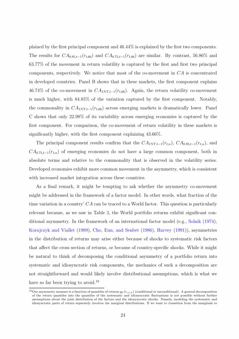
As a final remark, it might be tempting to ask whether the asymmetry co-movement

might be addressed in the framework of a factor model. In other words, what fraction of the

time variation in a country’ CA can be traced to a World factor. This question is particularly

relevant because, as we saw in Table 3, the World portfolio returns exhibit significant con-

ditional asymmetry. In the framework of an international factor model (e.g., Solnik (1974),

Korajczyk and Viallet (1989), Cho, Eun, and Senbet (1986), Harvey (1991)), asymmetries

in the distribution of returns may arise either because of shocks to systematic risk factors

that affect the cross section of returns, or because of country-specific shocks. While it might

be natural to think of decomposing the conditional asymmetry of a portfolio return into

systematic and idiosyncratic risk components, the mechanics of such a decomposition are

not straightforward and would likely involve distributional assumptions, which is what we

have so far been trying to avoid.19

19Our asymmetry measure is a function of quantiles of returns qθ (ri,t,n) (conditional or unconditional). A general decompositionof the return quantiles into the quantiles of the systematic and idiosyncratic fluctuations is not possible without furtherassumptions about the joint distribution of the factors and the idiosyncratic shocks. Namely, modeling the systematic andidiosyncratic parts of return separately involves the marginal distributions. If we want to transition from the marginals to

24

4.3 Conditional Asymmetry, Volatility, and U.S. Recessions

In this section, we address the following two questions. First, do we observe more negative

skewness in periods of high volatility? This question is motivated by a large body of literature

that has established a relation between higher volatility and negative returns in the U.S. stock

market. The finding, known as the “leverage effect”, has been documented using various

statistical approaches. We revisit it here for a couple of reasons. Replicating this stylized

fact with the CAINT,t−1(rt,n) and CAθ,t−1(rt,n) measures would lend further credence that

we are capturing conditional asymmetry in returns. Moreover, while the leverage effect has

been established for the U.S. and some DMs, whether it is present in EM returns is less

clear. For instance, Bekaert and Harvey (1997) do not find support for the leverage effect in

a limited sample of emerging economies.

Second, are the asymmetries more pronounced during U.S. recessions? From an U.S. in-

vestor’s perspective, which we adopt in the next section, understanding whether CAθ,t−1(rt,n)

and CAINT,t−1(rt,n) co-vary with U.S. investment opportunities is important for hedging. We

expect the U.S. stock market return asymmetry to be more pronounced during U.S. reces-

sions. Relative to the U.S. stock market, we also expect the CAs in other markets to be less

affected by downturns in the U.S. economy. It is this difference in markets’ response to U.S.

recessions that might provide hedging opportunities to investors. We use U.S. recessions

dates provided by the National Bureau of Economic Research (NBER).

To tackle these questions, we estimate the model:

CAt−1(rt,n,i) = a + b1σt−1,n,i + b2NBERt−1 + ǫt,n,i (10)

where σt−1,n,i denotes the n-period return volatility of country i, estimated with a MIDAS

regression as in the previous section. The index variable NBERt−1 is equal to one if month

t − 1 falls in a recession as defined by the NBER. The left-hand side variable is either

CAINT,t−1(rt,n,i), CA0.95,t−1(rt,n,i), or CA0.75,t−1(rt,n,i). The regression is estimated in the

time-series for the U.S., China, and World portfolio. For the group of DM ex-U.S. and

the joint distribution of returns, we have to take a stand on the dependence between these two marginal distributions. Oneway of doing this would be through some parametric assumptions, such as a copula function. However, this would involvemaking distributional assumptions, and would critically depend on the choice of copula.

25

EM ex-China, we pool the observations across countries and months, and compute clustered

standard errors.

The monthly and quarterly results are presented in Table 4. Consistent with the leverage

effect literature, we observe a negative relation between the CAINT,t−1(rn,i,t) and volatility at

monthly horizons (Panel A). The coefficient in front of volatility is significant at the 1% for

the U.S. and China, and at the 10% for the World portfolio. The leverage effect seems to be

present and quite pronounced in emerging economies in terms of magnitude and statistical

significance. The volatility coefficient estimates for EM countries (China and EM ex-China)

are larger in magnitude than in DM countries. The quarterly results in Panel B carry the

same message as the leverage effect is present in DM and EM economies. The parameter

estimates on volatility are larger in magnitude than in Panel A and significant at the 1% level

in all columns but DM ex-U.S.. The same holds true for CAINT,t−1(rt,n,i), CA0.95,t−1(rt,n,i),

as well as CA0.75,t−1(rt,n,i).

U.S. stock market returns are generally more negatively skewed during U.S. downturns. In

the monthly CAINT,t−1(rt,22,i) regressions (Panel A of Table 4), the coefficient on the NBER

dummy is negative and significant with a p-value of 0.03. At quarterly frequency (Panel B),

the coefficient is negative, larger in magnitude, and significant at the 6% level. Given the low

power of the t-test with these dummy variables (there are only 4 recessions in our sample)

it is encouraging to detect statistical significance. The negative effect is still present in the

CA0.95,t−1(rt,n,i) and CA0.75,t−1(rt,n,i) regressions, is not significant at monthly frequency, and

is significant at quarterly horizons. Hence, for monthly returns, the effect must largely be

due to the extreme quantiles that enter in the construction of CAINT,t−1(rt,n,i).

By contrast, U.S. recessions have little to no impact on the asymmetry regressions for

China, DM ex-U.S., and EX ex-China. This is true for CAINT,t−1(rt,n,i), CA0.95,t−1(rt,n,i),

and CA0.75,t−1(rt,n,i) in Panels A and B. The coefficients in World portfolio regressions are

mostly negative and insignificant. These insignificant results might be somewhat surprising,

given the financial markets integration especially among DM countries. To understand them,

it is useful to recall that market integration has thus far been linked to the first and second

moment of returns (e.g., Bekaert and Harvey (1995)). As discussed in section 3, however, the

CA measures ought not to be affected by variations in the conditional mean and variance.

26

Moreover, regression (10) controls explicitly for country volatility. Hence, the findings in

Table 4 suggest that, above and beyond mean-variance effects, U.S. recessions do not impact

non-U.S. markets return asymmetry. This is again in line with the lack of commonality

across country CAs that we documented above.

5 International Portfolio Allocation: Exploiting Con-

ditional Return Asymmetry

The benefits of international diversification and the related topic of global market inte-

gration have been mostly framed in the context of modeling the time varying means and

covariance matrix of stock returns.20 To capture the gist of that literature – and at risk of

over-simplifying a complex subject – in Panel A of Figure 5 we display the average rolling

correlation of monthly returns among DM countries (dotted line), among EM countries

(dash-dotted line), and between EM and DM countries (solid line). The plots illustrate why

it is often argued that the benefits of international diversification are limited and decreasing

(Christoffersen, Errunza, Jacobs, and Jin (2012)). The average correlation across DM re-

turns increases over our sample to as high as 0.90, and even the average correlation between

DM and EM countries is trending up over time and is currently about 0.50.

The correlation in returns differs markedly from that of the asymmetry measure. Panel

B of Figure 5 displays the average correlations of CAINT (rt,22) across DM, across EM, and

between DM and EM economies. The plot confirms the conclusions that already emerged

from Figure 4 and section 4.2, namely, return asymmetries of emerging and developed mar-

kets exhibit little significant co-movement. In contrast with Panel A, there are virtually no

trends in the CAINT (rt,22) correlations throughout the sample. In an international portfo-

lio context, Figure 5 suggests that investors can improve upon the standard mean-variance

allocation by taking into account features of the return distribution, such as asymmetries,

while making optimal portfolio decisions (Guidolin and Timmermann (2008) and Jondeau

and Rockinger (2006)). However, incorporating return asymmetry in an optimal portfolio

20Among the many papers on the topic, see Solnik (1974), Stulz (1981, 1987), Korajczyk and Viallet (1989), King, Sentana, andWadhwani (1994), Bekaert and Harvey (1995), Harvey (1995), Bekaert and Harvey (1997), Pukthuanthong and Roll (2009),Engle and Rangel (2008).

27

setting and quantifying its benefits is not a simple task. The direct approach of modeling

the joint conditional return distribution of 73 countries is practically speaking not possible,

especially since we only have at most 30 years of data. One way of circumventing the prob-

lem of dimensionality is by modeling the non-linear dependence between pairs of countries

as in Christoffersen, Errunza, Jacobs, and Jin (2012).

In this paper, we adopt the parametric portfolio approach of Brandt, Santa-Clara, and

Valkanov (2009), which consists of specifying the portfolio weights as a function of asset-

specific characteristics. Specifically, Brandt, Santa-Clara, and Valkanov (2009) investigate

whether U.S. firm characteristics (such as size, value, and momentum) can lead to sizeable

portfolio improvements relative to the benchmark value-weighted portfolio. In the current

context, our main objective is to answer whether an investor can exploit the documented

differences and variations in DM and EM return asymmetries by tilting her portfolio toward

positively skewed (or less negatively skewed) country returns. And, if so, how large would

the resulting portfolio gains be? Since the parametric portfolio approach is fairly novel and

has to be modified for our application, we briefly describe it below.

5.1 Methodology

We investigate whether and to what extent the estimated conditional return asymmetry mea-

sures CAINT,t−1(rt,n,i) and CAθ,t−1(rt,n,i) could alter a representative investor’s optimal asset

allocation across 73 country returns relative to the natural benchmark–the value-weighted

World portfolio return. As in the previous section, let the subscript i denote a given coun-

try and Nt−1 be the number of countries in the sample at time (month or quarter) t − 1.

We simplify notation by dropping the horizon subscript n, while keeping in mind that the

portfolio allocation results will be presented at monthly and quarterly frequencies.

An investor chooses portfolio weights wt−1,i to maximize the conditional expected utility

of her portfolio return rt,p,

max{wt−1,i}

Nt−1

i=1

Et−1 [u (rt,p)] (11)

where rt,p =∑Nt−1

i=1 wt−1,irt,i. Following Brandt, Santa-Clara, and Valkanov (2009), we specify

28

the portfolio weights of each country as a linear function of the CA measure:

wt−1,i = wt−1,i + φ1

Nt−1CAt−1(rt,i)

= wt−1,i + wCAt−1,i (12)

where wt−1,i is the weight of country i in the value-weighted (market) portfolio and CAt−1(rt,i)

is the asymmetry measure of country i, standardized to have mean zero and unit standard

deviation at each t. The normalization 1/Nt−1 allows the number of countries to vary across

periods.

The weights in expression (12) are estimated by maximizing objective function (11) with

respect to the parameter φ. Standardizing CAt−1(rt,i) ensures that∑

i wCAt−1,i = 0. This

allows us to interpret the estimated wCAt−1,i as the “actively managed” allocation in a long-

short portfolio that tilts the optimal weight in country i toward or away from wt−1,i depending

on that country’s CAt−1(rt,i) relative to the cross-sectional mean. For instance, if the investor

prefers positive skewed assets and the true value of the parameter φ is positive, then countries

with higher (lower) CAt−1(rt,i) will have a higher (lower) portfolio weight than in the value-

weighted portfolio.

Solving for the optimal portfolio policy in (11) allows us to understand how do the

performance and holdings change when conditional asymmetry is taken into account. We

obtain this result by decomposing the portfolio return based on (12) as:

rt,p = rt,p + rCAt,p (13)

Here, rt,p =∑Nt−1

i=1 wt−1,irt,i is the value-weighted market return while rCAt,p =

∑Nt−1

i=1 wCAt−1,irt,i

is the return of the actively-managed portfolio, which measures the economic impact of

conditioning on CA.

The portfolio approach also enables us to keep track of whether the holdings are in

developed versus emerging economies as:

rt,p = rt,DM + rt,EM . (14)

29

In this expression, rt,DM =∑

i 1DMi wt−1,irt,i is the return attributable to developed markets

and rt,EM is defined similarly. The decomposition is based on∑

i wt−1,i = wt−1,DM+wt−1,EM ,

where wt−1,DM =∑

i 1DMi wt−1,i, wt−1,EM =

∑i 1

EMi wt−1,i and 1DM

i (1EMi ) is a dummy

variable that equals one if country i is developed (emerging), and zero otherwise.21 Moreover,

combining expressions (13) and (14), we obtain

rt,p = rt,p + (rCAt,DM + rCA

t,EM) (15)

The impact of CAt−1(rt,i) on the portfolio allocation is captured by the actively-managed

weights wCAt−1,DM and wCA

t−1,EM . They reflect the net re-balancing between developed and

emerging markets, as wCAt−1,DM + wCA

t−1,EM = 0 (because CAt−1(rt,i) is standardized cross-

sectionally). We report these weights, the returns associated with the re-balancing, rCAt,DM

and rCAt,EM , and also their correlation ρ

(rCAt,DM , rCA

t,EM

). The total correlation between the DM

and EM returns, ρ (rDM,t, rEM,t), which is affected by fluctuations in market weights, is also

discussed.

The parametric weight function in (12) can be easily generalized to include other con-

ditioning information by letting wt−1,i = wt−1,i + φ 1Nt−1

CAt−1(rt,i) + ξ′ 1Nt−1

Ht−1,i = wt−1,i +

wCAt−1,i + wH

t−1,i, where Ht−1,i is a vector of country-specific characteristics, and ξ is a vector

of coefficients to be estimated. We are interested in wCAt−1,i which is the part of the weights

due solely to fluctuations in CAt−1,i.

5.2 International Portfolio Results

We estimate the parametric portfolio weights (12) by maximizing the sample analogue of the

expected utility (11) with respect to the parameters of interest. In Tables 5 and 6 we present

the results for a power utility investor with a coefficient of relative risk aversion γ = 5 who

re-balances her portfolio over the entire panel of 73 countries monthly (Panel A) or quarterly

(Panel B). Our main conclusions hold for a range of risk aversion parameters and we present

those results in a robustness section. The benchmark value-weighted weights are computed

based on countries’ stock market capitalizations at the end of the previous year.

21Note that rt,DM and rt,EM are not proper portfolio returns as their weights do not sum up to one. Rather, they arecomponents of rt,p that are attributable to developed versus emerging countries.

30

Table 5 displays the estimation results for eight specifications of the portfolio weights

(12) or its generalization. In columns (1)-(3), we include the measures CAINT,t−1(rt,n),

CA0.95,t−1(rt,n), and CA0.75,t−1(rt,n), separately. The conditional asymmetry has a sig-

nificant impact on the portfolio allocation at monthly and quarterly horizons. Namely,

CAINT,t−1(rt,n) enters with the expected positive sign and is significant at the 1% level. In

the quarterly results, a country with a CAINT,t−1(rt,n) 1 standard deviation higher than the

cross-sectional mean ought to have a 2.391% higher weight in the optimal portfolio than in

the value-weighted portfolio. The results are even stronger for the monthly horizons, because

the CAINT,t−1(rt,22) estimates are more variable than the CAINT,t−1(rt,66).

We observe that most of the significance comes from the tails of the distribution. Com-

paring the CA0.95,t−1(rt,n) and CA0.75,t−1(rt,n) results, the estimates are larger in magnitude

and statistically significant for the 0.95 quantile. The coefficient on CA0.75,t(rt,n), while pos-

itive, is insignificant at monthly and quarterly frequencies. These results suggest that, from

an international portfolio perspective, asymmetries in the tail of the distribution of returns

can be used to improve upon the benchmark value-weighted portfolio.

In specifications (4)-(8), we include conditional volatility, expected moment-based skew-

ness, co-skewness, and interaction with NBER recessions as additional controls in the para-

metric portfolio weights. The last column includes both CA0.95,t(rt,n) and CA0.75,t(rt,n) in

addition to all controls. Expected skewness is computed as the fitted value from regressing

the future realized skewness of n-day returns on conditional volatility and lagged 250-day

skewness, similarly to Boyer, Mitton, and Vorkink (2010). Co-skewness obtains from re-

gressing (lagged) 250-day country returns on the contemporaneous squared returns to the

World portfolio. Note that all our conditioning variables are based on the same information

set of lagged, 250 daily returns thus allowing proper comparisons. While the value-weighted

benchmark should already account for the risk captured in the volatility of country returns

(i.e., the value-weighted portfolio should be close to mean-variance efficient), we control

for volatility because time-variations in the second moment might give rise to short-term

re-balancing opportunities. By including country volatility in the parametric portfolio func-

tion, we also rule out the possibility that the CA measures might simply be proxying for

volatility given the above-documented negative volatility-conditional asymmetry correlation

31

(leverage effect).

The inclusion of additional controls does not significantly alter the coefficients of CAINT,t−1(rt,n)

and CA0.95,t−1(rt,n) nor their significance. The estimates in front of volatility have the ex-

pected negative sign, but are insignificant at the monthly horizon. Volatility is significant

at quarterly horizons only in the CA0.75,t−1(rt,n) specification. The interaction with NBER

recessions does not seem to play a significant role in the optimal allocation at any horizon.

This implies that the portfolio gains of conditioning on CA are not purely concentrated

around recession times. Expected skewness has the expected positive sign in all specifica-

tions in Panels A and B. At monthly frequency, it is insignificant in the specification with

CAINT,t−1(rt,n) and CA0.95,t−1(rt,n), but the magnitude of its coefficients are about two-

thirds smaller. However, it is significant at quarterly horizons for most of the specifications.

Co-skewness, on the other hand, is not significant at any horizon in any of the specifications.

Table 6 presents the allocation and performance of the same eight specifications at

monthly and quarterly frequencies. In each panel, we first report time-series averages of

the weights wt−1,i and their decompositions, then of returns and their decompositions, and

finally risk and portfolio performance statistics. All returns are annualized to facilitate com-

parison across horizons. As a benchmark, the first column “VW” displays the properties of

the value-weighted portfolio. In it, the average weight placed on emerging markets wEM is

9.290% and the average total return rp of 7.7% is mostly due to the performance of developed

markets (rDM).22 The annualized volatility of the value-weighted portfolio is 16.3% and its

skewness is −1.038.

Exploiting CAINT,t−1(rt,22) shifts the monthly portfolio allocation significantly toward

emerging markets. In specification (1), the average EM weight is 47%, which is about five

times higher that in the value-weighted allocation. The average portfolio return increases to

14.6%, with all the gains coming from EM markets (7.2%). The correlation between the EM

and DM components is close to zero (−0.072). Since specification (1) has only one condition-

ing variable, CAINT,t−1(rt,n), the average EM returns attributable to CAINT,t−1(rt,n) fluctu-

ations (rCAEM) is 7.2% whereas for DM indices it is negligible (−0.003). In other words, the

22This finding can be explained as follows. EM have positive average returns in our sample (see Table 1), but their weight inthe VW portfolio increases in significance just in the latter part of the sample, when realized returns happen to be low.

32

optimal portfolio weights successfully exploit the favorable asymmetry in emerging markets.

The volatility of the optimal portfolio (16%) is actually lower than that of the value-weighted

benchmark and its certainty equivalent return is 8.4%. Importantly, the optimal portfolio

moment-based skewness is now positive at 0.501 whereas it is −1.038 in the value-weighted

portfolio. The increased skewness of the optimal portfolio is a good check that conditioning

on CAINT,t−1(rt,22) has the expected effect and is further confirmation that CAINT,t−1(rt,22)

is a proper measure of return asymmetry.

The results for CA0.95,t−1(rt,n) in column (2) are similar to those in column (1). The

resultant optimal portfolio allocates about 40% of the portfolio weight into EM countries,

and its return and volatility are 16.5% and 17.0%, respectively. Most of the gains are again

attributable to EM countries (rEM is 0.082) and the correlation between the EM and DM

components of the return is −0.152. The CA0.75,t−1(rt,n) results in column 3 are markedly

different, mirroring the low and statistically insignificant coefficient in front of CA0.75,t−1(rt,n)

in Table 5.

The properties of the optimal portfolio are not significantly altered by the inclusion of

country volatility, expected skewness, and co-skewness. In specifications (4), (5), (7), and

(8) the portfolio weight in EM is between 41.621% and 48.335%. The portfolio returns in

those specifications are in the 15% to 21% range, the volatility is between 16% and 19.6%,

and the certainty equivalent return is between 9% and 10%. Interestingly, the gains in

these portfolios can mostly be traced to the CA measures rather than to the other controls.

To see that in specification (4), we compare the average active returns from EM countries

rEM of 8.6% to the average rCAEM of 7.0%. The first return captures the joint impact of all

controls whereas the second one isolates the contribution of the CA measure in the return

decomposition. Similar results hold for specifications (5), (7), and (8).

The use of CA0.75,t−1(rt,n) in columns (3) and (6) does not lead to important portfolio im-

provements. The performance gains are lower than for the other two measures, the weight on

EM is lower, and so is the certainty equivalent return. By contrast, including CA0.95,t−1(rt,n)

and CA0.75,t−1(rt,n) jointly (specification (8)) raises the optimal portfolio performance, the

weights on EM, and the certainty equivalent return. This is perhaps the most convincing

evidence that asymmetries are exploitable in an international portfolio context as long as

33

they are in the tails of the distribution.

The quarterly results in Panel B of Table 6 are similar with a few qualifications. The

use of CAINT,t−1(rt,66) and CA0.95,t−1(rt,66) increases the average weight in emerging markets

from 9.161% to between 23% and 39%. The somewhat lower weight on EM is attributable to

the lower volatility of the quarterly CA statistics. While the portfolio returns and certainty

equivalent return are somewhat lower than in the monthly case, they are still economically

meaningful. For instance, the certainty equivalent return in all specifications excluding (3)

and (6) are between 3.1% to 8.8% higher than that of the value-weighted benchmark, which

is practically zero (−0.009).

In Figure 6, we display the time-series of the quarterly optimal portfolio weights wt−1,EM

and wCAt−1,EM in specification (6). In Panel A, we see a clear upward drift in wt−1,EM which im-

plies that the optimal portfolio allocates a larger fraction of the overall holdings to emerging

markets. Part of that increase is due to the fact that emerging stock markets are growing

faster than some developed markets and are getting a larger share in the value-weighted

portfolio. Another part is due to the pure conditional asymmetry effect, which is captured

in wCAt−1,EM and displayed in Panel B. The positive albeit not as pronounced trend in wCA

t−1,EM

implies that the gains from exploiting conditional asymmetry in emerging markets are quite

stable and persistent over time. Finally, we include in the plot the minimum and maximum

weights across EM on a given quarter. For the optimal CA weights, these vary in the -0.10

to 0.10 range implying that short and long positions in any given country do not exceed 10%

of the value of the portfolio. This evidence is rather reassuring that the gains we document

in Table 6 do not emerge from the investor taking disproportionately large positions in a

small number of countries.

Overall, the evidence in Tables 5, 6 and Figure 6 convey a uniform message: conditioning

on CAINT,t−1(rt,n) and CA0.95,t−1(rt,n) improves the portfolio allocation by tilting the port-

folio toward emerging economies, because their returns tend to be less negatively skewed.

Asymmetries that are not in the tail of the return distribution have little effect on portfolio

allocation decisions.

34

5.3 Additional Analysis and Robustness

We perform a series of checks to verify that the portfolio results are robust to the choice

of the risk aversion parameter, to de-TARCHing the returns, and to an alternative dataset.

The results are presented in Table 7 for monthly returns following the format of Tables 5

and 6. For conciseness, we display only the loading on CAINT,t−1(rt,n) corresponding to

specification (7) of Table 5.

Different degree of relative risk aversion: We estimate the optimal portfolio policy

for γ of 3, 10, and 20. The results are displayed in columns (1), (3), and (4) respectively.

The benchmark γ = 5 from Table 5 is also reported in column (2) to facilitate the compari-

son. The CAINT,t−1(rt,n) measure is always significant, more so when the investor is less risk

averse. This is expected as low γ investors are able to better exploit fluctuations in condi-

tional asymmetry. Investors with a γ of 20 and 10 hold on average between 29% and 36% of

their portfolio in emerging economies, which is significantly larger than the value-weighted

weight of about 9%. In all specifications, the correlations between the EM and DM returns

is close to zero. The certainty equivalent return and alpha of the optimal portfolio decrease

as the risk aversion increases.

Volatility-Filtered Returns: We saw in section 3.4 that there are significant dynamics

in the quantiles of de-TARCHed returns. However, the question remains whether the condi-

tional asymmetry in the de-TARCHed returns is substantial enough to matter in an interna-

tional portfolio context. To this end, we compute the optimal portfolio weights conditioning

on CAINT,t−1(rt,n) estimated from the quantiles of de-TARCHed returns in section 3.4. The

results are reported for γ = 5 in column (5) of Table 7. The coefficient of CAINT,t−1(rt,n)

is statistically significant and very similar to that of the unfiltered series (column (2)). This

result is not unexpected if we recall that the quantiles of the filtered and unfiltered returns

are highly correlated.

Investable indices: Is the predicted optimal portfolio a truly achievable investment strat-

egy? This issue is relevant for international portfolio allocation as foreigners cannot invest in

country indices in an unrestricted fashion. To address this concern, following Christoffersen,

Errunza, Jacobs, and Jin (2012), we rely on Emerging Markets S&P IFCI indices, which

35

track the return a foreign investor is legally able to achieve through investment in a country

domestic equity. For Developed Markets, we use FTSE indices. The use of this series reduces

considerably our time span as the data start on July 3, 1995. We also have a smaller cross

section. All developed markets but Iceland are in this sample, but we only have a subset of

19 out of the 48 emerging countries.23

We estimate the conditional asymmetry and the dynamic portfolio policy problem at

the monthly horizon for this new dataset and report the results in column (5). The role

of conditional asymmetry remains significant and economically strong. In particular, the

loading on CAINT is now 4.050 (compared to 2.988 in column (2)) with a certainty equivalent

return of 0.099 (versus 0.091). The fraction invested in emerging markets due to conditional

asymmetry remains substantially larger than in the value-weighted portfolio figure (which is

about 5%). This evidence clarifies that our results are not driven by positions in very small

countries that may be in practice out-of-reach.

6 Conclusions

We use a new approach to estimate the conditional asymmetry in portfolio returns at dif-

ferent points of the distribution and study a large cross-section of developed and emerging

markets. Estimates of CA reveal several novel results such as significant dynamics over time,

heterogeneity across countries, a low correlation between asymmetries of DM and EM port-

folio returns, and negative correlation with the conditional volatility. These findings have

significant implications for international asset allocation and risk sharing, some of which

are explored in this paper. Namely, employing a parametric portfolio approach to study

the impact of return asymmetry on the asset allocation across 73 countries, we find that the

optimal portfolio is tilted toward countries that are less negatively skewed, which in our sam-

ple are the emerging economies. In other words, the introduction of conditional asymmetry

results in the optimal portfolio placing a significantly larger weight on emerging economies

than does the value-weighted portfolio.

Our empirical findings suggest a rich agenda for future research. First, the low correlation

23These countries tend to have mature and liquid markets. They are: Brazil, Chile, China, Czech Republic, Egypt, Hungary,India, Indonesia, Malaysia, Mexico, Morocco, Peru, Philippines, Poland, Russia, South Africa, Taiwan, Thailand, and Turkey.

36

in CAs prompts questions about its economic provenance and significance. Exploring the

role of global and country-specific macroeconomic shocks in driving the conditional asym-

metry in returns might prove particularly insightful. Moreover, while we do not directly link

expected returns and conditional asymmetry, an explicit investigation of this relation, fol-

lowing Boyer, Mitton, and Vorkink’s (2010) work on U.S. data, would be of great importance

for international asset pricing. Finally, our investigation focuses primarily on monthly and

quarterly returns, but it also suggests that the term structure of conditional skewness may

provide new insights into the measures of risk at different horizons. While we know remark-

ably little about this topic, the current mixed-data approach offers a tractable framework

for further explorations.

37

References

Andreou, Elena, Eric Ghysels, and Andros Kourtellos, 2011, Forecasting with Mixed-Frequency Data, in M. P. Clements, and D. F. Hendry, ed.: Oxford Handbook of EconomicForecasting. Oxford University Press.

Armesto, Michelle T., Kristie M. Engenmann, and Michael T. Owyang, 2010, Forecastingwith mixed frequencies, Federal Reserve Bank of St. Louis Review 92, 521–536.

Barberis, Nicholas, and Ming Huang, 2008, Stocks as Lotteries: The Implications of Proba-bility Weighting for Security Prices, American Economic Review 98, 2066–2100.

Bekaert, Geert, and Campbell R. Harvey, 1995, Time-Varying World Market Integration,Journal of Finance 50, 403–444.

, 1997, Emerging Equity Market Volatility, Journal of Financial Economics 43, 29–77.

, Christian Lundblad, and Stephan Siegel, 2011, What Segments Equity Markets?,Review of Financial Studies 24, 3847–3890.

Bowley, Arthur, 1920, Elements of Statistics (Charles Scribner’s Sons: New York).

Boyer, Brian, Todd Mitton, and Keith Vorkink, 2010, Expected Idiosyncratic Skewness,Review of Financial Studies 23, 169–202.

Brandt, Michael, 2010, Portfolio choice problems, in Y. Ait-Sahalia, and L.P. Hansen, ed.:Handbook of Financial Econometrics, Volume 1: Tools and Techniques pp. 269–336. NorthHolland.

, Pedro Santa-Clara, and Rossen Valkanov, 2009, Parametric Portfolio Policies: Ex-ploiting Characteristics in the Cross Section of Equity Returns, Review of Financial Stud-ies 22, 3411–3447.

Brunnermeier, Markus, Christian Gollier, and Jonathan Parker, 2007, Optimal Beliefs, AssetPrices and the Preference for Skewed Returns, American Economics Review (Papers andProceedings) 97, 159–165.

Campbell, John, and Luis Viceira, 2002, Strategic Asset Allocation: Portfolio Choice forLong-Term Investors (Oxford University Press).

Campbell, John Y., and Ludger Hentschel, 1992, No News is Good News: An AsymmetricModel of Changing Volatility in Stock Returns, Journal of Financial Economics 31, 281–318.

Chang, B., Peter Christoffersen, and Kris Jacobs, 2013, Market Skewness Risk and theCross-Section of Stock Returns. , 107, 46-68., Journal of Financial Economics 107, 46–68.

Chen, Joseph, Harrison Hong, and Jeremy Stein, 2001, Forecasting Crashes: Trading Vol-ume, Past Returns, and Conditional Skewness in Stock Prices, Journal of Financial Eco-nomics 61, 345–381.

Chernozhukov, Victor, Ivan Fernandez-Val, and A. Galichon, 2010, Quantile and ProbabilityCurves without Crossing, Econometrica 78, 1093–1125.

Cho, D. Chinhyung, Cheol S. Eun, and Lemma W. Senbet, 1986, International ArbitragePricing Theory: An Empirical Investigation, Journal of Finance 41, 313–329.

38

Christoffersen, Peter, Vihang R. Errunza, Kris Jacobs, and Xisong Jin, 2012, Is the Potentialfor International Diversification Disappearing?, Review of Financial Studies 25, 3711–3751Discussion Paper, University of Toronto.

Conrad, Jennifer, Robert Dittmar, and Eric Ghysels, 2013, Ex Ante Skewness and ExpectedStock Returns, Journal of Finance 68, 85–124.

DeMiguel, Victor, Yuliya Plyakha, Raman Uppal, and Grigory Vilkov, 2013, ImprovingPortfolio Selection using Option-implied Volatility and Skewness, Journal of Financialand Quantitative Analysis, forthcoming.

Dette, Holger, and Stanislav Volgushev, 2008, Non-crossing Non-parametric Estimates ofQuantile Curves, Journal of the Royal Statistical Society: Series B (Statistical Methodol-ogy) 70, 609–627.

Engle, Robert, and Simone Manganelli, 2004, CAViaR: COnditional Autoregressive Value atRisk by Regression Quantiles, Journal of Business and Economic Statistics 22, 367–381.

Engle, Robert, and Abhishek Mistry, 2007, Priced Risk and Asymmetric Volatility in theCross-Section of Skewness, Working Paper, NYU Stern School of Business.

Engle, Robert, and Jose Gonzalo Rangel, 2008, The Spline-GARCH Model for Low-Frequency Volatility and Its Global Macroeconomic Causes, Review of Financial Studies21, 1187–1222.

Fama, Eugene F., and Kenneth R. French, 1998, Value versus Growth: The InternationalEvidence, Journal of Finance 53, 1975–1999.

Ghysels, Eric, 2013, Matlab Toolbox for Mixed Sampling Frequency Data Analysis usingMIDAS Regression Models - Version 8, Available at http://www.unc.edu/~eghysels.

, Pedro Santa-Clara, and Rossen Valkanov, 2005, There is a Risk-Return TradeoffAfter All, Journal of Financial Economics 76, 509–548.

, 2006, Predicting Volatility: Getting the Most out of Return Data Sampled atDifferent Frequencies, Journal of Econometrics 131, 59–95.

Ghysels, Eric, Arthur Sinko, and Rossen Valkanov, 2006, MIDAS Regressions: Further Re-sults and New Directions, Econometric Reviews 26, 53–90.

Ghysels, Eric, and Rossen Valkanov, 2011, Volatility Prediction with MIDAS, in L. Bauwens,C. Hafner, and S. Laurent, ed.: Wiley Handbook Volatility Models and Their Applications.Wiley (forthcoming).

Glosten, Larry R., Ravi Jagannathan, and David E. Runkle, 1993, On the Relation Betweenthe Expected Value and the Volatility of the Nominal Excess Return on Stocks, Journalof Finance 48, 1779–1801.

Groeneveld, Richard, and Glen Meeden, 1984, Measuring Skewness and Kurtosis, The Statis-tician 33, 391–399.

Guidolin, Massimo, and Allan Timmermann, 2008, International Asset Allocation underRegime Switching, Skew, and Kurtosis Preferences, Review of Financial Studies 21, 889–935.

Harvey, Campbell R., 1991, The World Price of Covariance Risk, Journal of Finance 46,111–157.

39

, 1995, Predictable Risk and Returns in Emerging Markets, Review of FinancialStudies 8, 773–816.

, John C. Liechty, Merrill W. Liechty, and Peter Muller, 2010, Portfolio selectionwith higher moments, Quantitative Finance 10, 469–485.

Harvey, Campbell R., and Akhtar Siddique, 1999, Autoregressive Conditional Skewness,Journal of Financial and Quantitative Analysis 34, 465–487.

Henry, Peter B., 2000, Stock Market Liberalization, Economic Reform, and Emerging MarketEquity Prices, Journal of Finance 55, 529–564.

Hinkley, David V., 1975, On Power Transformations to Symmetry, Biometrika 62, 101–111.

Hong, Harrison, and Jeremy C. Stein, 2003, Differences of Opinion, Short Sales Constraints,and Market Crashes, Review of Financial Studies 16, 487–525.

Jondeau, E., and M. Rockinger, 2006, Optimal Portfolio Allocation under Higher Moments,European Financial Management 12, 29–55.

Kim, Tae-Hwan, and Halbert White, 2004, On More Robust Estimation of Skewness andKurtosis, Finance Research Letters 1, 56–70.

King, Mervyn, Enrique Sentana, and Sushi Wadhwani, 1994, Volatility and Links betweenNational Stock Markets, Econometrica 62, 901–933.

Koenker, Roger, and George Bassett, 1978, Regression Quantiles, Econometrica 46, 33–50.

Koenker, Roger, and Zhijie Xiao, 2006, Quantile Autoregression, Journal of the AmericanStatistical Association 101, 980–990.

Korajczyk, Robert, and Claude Viallet, 1989, An Empirical Investigation of InternationalAsset Pricing, Review of Financial Studies 2, 553–585.

Kraus, Alan, and Robert Litzenberger, 1976, Skewness Preference and the Valuation of RiskAssets, Journal of Finance 31, 1085–1100.

, 1983, On the distributional conditions for a consumption-oriented three momentcapm, The Journal of Finance 38, pp. 1381–1391.

Kupiec, Paul, 1995, Techniques for Verifying the Accuracy of Risk Measurement Models,Journal of Derivatives 2, 73–84.

Leon, Angel, Gonzalo Rubio, and Gregorio Serna, 2005, Autoregressive Conditional Volatil-ity, Skewness and Kurtosis, Quarterly Review of Economics and Finance 45, 599–618.

Neuberger, Anthony, 2012, Realized skewness, Review of Financial Studies 25, 3423–3455.

Newey, Whitney K., and Kenneth D. West, 1987, A simple positive semi-definite, het-eroskedasticity and autocorrelation consistent covariance matrix, Econometrica 55, 703–708.

Pearson, Karl, 1895, Contributions to the Mathematical Theory of Evolution. II. Skew Varia-tion in Homogeneous Material, Philosophical Transactions of the Royal Society of London.A 186, 343–414.

Pukthuanthong, Kuntara, and Richard Roll, 2009, Global Market Integration: An Alterna-tive Measure and its Application, Journal of Financial Economics 94, 214–232.

40

, 2010, Internationally Correlated Jumps, UCLA Anderson School Working Paper.

Rubinstein, Mark E., 1973, The fundamental theorem of parameter-preference security val-uation, Journal of Financial and Quantitative Analysis 8, 61–69.

Solnik, Bruno, 1974, The International Pricing of Risk: An Empirical Investigation of theWorld Capital Market Structure, Journal of Finance 29, 48–54.

Stulz, Rene, 1987, An equilibrium model of exchange rate determination and asset pricingwith nontraded goods and imperfect information, Journal of Political Economy 95, 1024–1040.

Viceira, Luis, 2001, Optimal Portfolio Choice for Long-Horizon Investors with NontradableLabor Income, Journal of Finance 56, 433–470.

Weiss, Andrew A., 1991, Estimating Nonlinear Dynamic Models using Least Absolute ErrorEstimation, Econometric Theory 7, 46–68.

White, Halbert, 1996, Estimation, Inference and Specification Analysis (Cambridge Univer-sity Press: Cambridge).

, Tae-Hwan Kim, and Simone Manganelli, 2008, Modeling Autoregressive ConditionalSkewness and Kurtosis with Multi-Quantile CAViaR, in Robert F. Engle, and HalbertWhite, ed.: A Festschrift in Honor of Clive W.J. Granger. Oxford University Press.

41

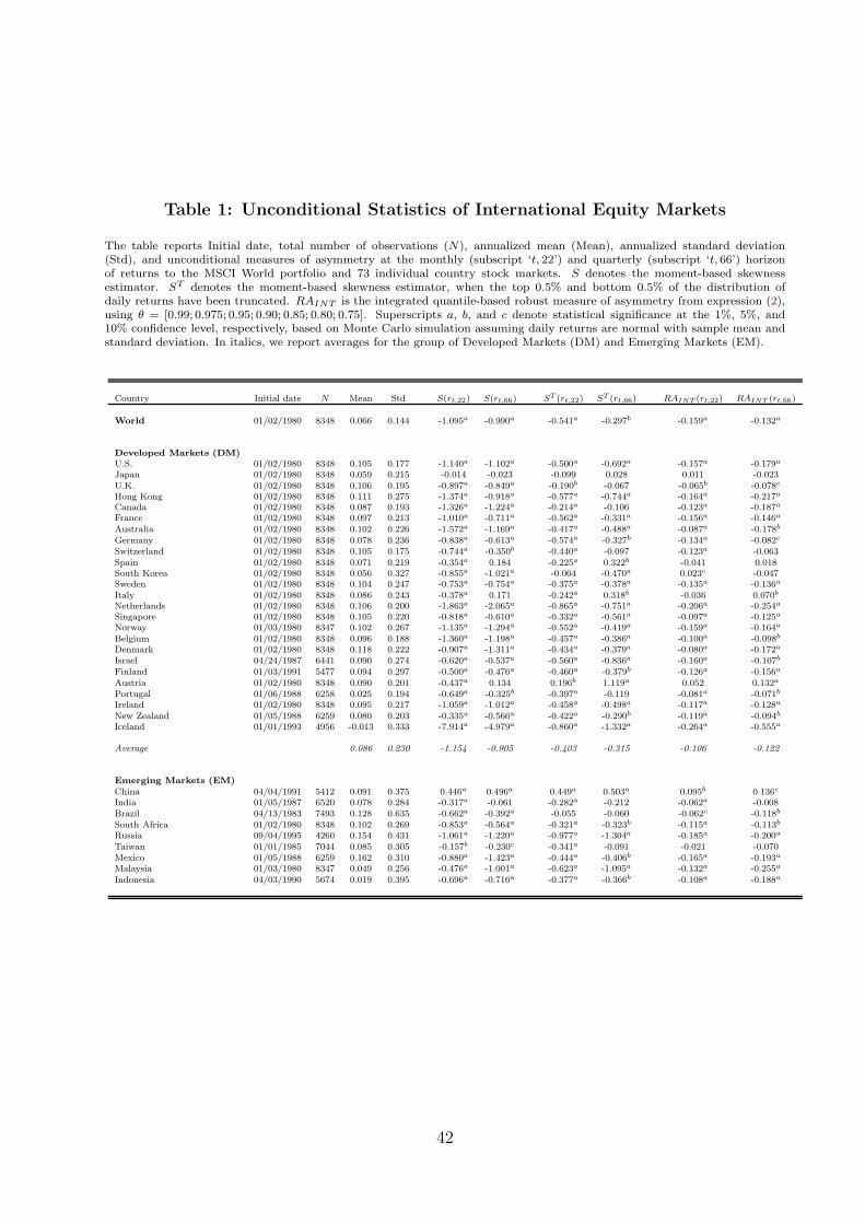
Table 1: Unconditional Statistics of International Equity Markets

The table reports Initial date, total number of observations (N), annualized mean (Mean), annualized standard deviation(Std), and unconditional measures of asymmetry at the monthly (subscript ‘t, 22’) and quarterly (subscript ‘t, 66’) horizonof returns to the MSCI World portfolio and 73 individual country stock markets. S denotes the moment-based skewnessestimator. ST denotes the moment-based skewness estimator, when the top 0.5% and bottom 0.5% of the distribution ofdaily returns have been truncated. RAINT is the integrated quantile-based robust measure of asymmetry from expression (2),using θ = [0.99; 0.975; 0.95; 0.90; 0.85; 0.80; 0.75]. Superscripts a, b, and c denote statistical significance at the 1%, 5%, and10% confidence level, respectively, based on Monte Carlo simulation assuming daily returns are normal with sample mean andstandard deviation. In italics, we report averages for the group of Developed Markets (DM) and Emerging Markets (EM).

Country Initial date N Mean Std S(rt,22) S(rt,66) ST (rt,22) ST (rt,66) RAINT (rt,22) RAINT (rt,66)

World 01/02/1980 8348 0.066 0.144 -1.095a -0.990a -0.541a -0.297b -0.159a -0.132a

Developed Markets (DM)U.S. 01/02/1980 8348 0.105 0.177 -1.140a -1.102a -0.500a -0.692a -0.157a -0.179a

Japan 01/02/1980 8348 0.059 0.215 -0.014 -0.023 -0.099 0.028 0.011 -0.023U.K. 01/02/1980 8348 0.106 0.195 -0.897a -0.849a -0.190b -0.067 -0.065b -0.078c

Hong Kong 01/02/1980 8348 0.111 0.275 -1.374a -0.918a -0.577a -0.744a -0.164a -0.217a

Canada 01/02/1980 8348 0.087 0.193 -1.326a -1.224a -0.214a -0.106 -0.123a -0.187a

France 01/02/1980 8348 0.097 0.213 -1.010a -0.711a -0.562a -0.331a -0.156a -0.146a

Australia 01/02/1980 8348 0.102 0.226 -1.572a -1.169a -0.417a -0.488a -0.087a -0.178b

Germany 01/02/1980 8348 0.078 0.236 -0.838a -0.613a -0.574a -0.327b -0.134a -0.082c

Switzerland 01/02/1980 8348 0.105 0.175 -0.744a -0.350b -0.440a -0.097 -0.123a -0.063Spain 01/02/1980 8348 0.071 0.219 -0.354a 0.184 -0.225a 0.322b -0.041 0.018South Korea 01/02/1980 8348 0.056 0.327 -0.855a -1.021a -0.064 -0.470a 0.023c -0.047Sweden 01/02/1980 8348 0.104 0.247 -0.753a -0.754a -0.375a -0.378a -0.135a -0.136a

Italy 01/02/1980 8348 0.086 0.243 -0.378a 0.171 -0.242a 0.318b -0.036 0.070b

Netherlands 01/02/1980 8348 0.106 0.200 -1.863a -2.065a -0.865a -0.751a -0.206a -0.254a

Singapore 01/02/1980 8348 0.105 0.220 -0.818a -0.610a -0.332a -0.561a -0.097a -0.125a

Norway 01/03/1980 8347 0.102 0.267 -1.135a -1.294a -0.552a -0.419a -0.159a -0.164a

Belgium 01/02/1980 8348 0.096 0.188 -1.360a -1.198a -0.457a -0.386a -0.100a -0.098b

Denmark 01/02/1980 8348 0.118 0.222 -0.907a -1.311a -0.434a -0.379a -0.080a -0.172a

Israel 04/24/1987 6441 0.090 0.274 -0.620a -0.537a -0.560a -0.836a -0.160a -0.107b

Finland 01/03/1991 5477 0.094 0.297 -0.500a -0.476a -0.460a -0.379b -0.126a -0.156a

Austria 01/02/1980 8348 0.090 0.201 -0.437a 0.134 0.196b 1.119a 0.052 0.132a

Portugal 01/06/1988 6258 0.025 0.194 -0.649a -0.325b -0.397a -0.119 -0.081a -0.071b

Ireland 01/02/1980 8348 0.095 0.217 -1.059a -1.012a -0.458a -0.498a -0.117a -0.128a

New Zealand 01/05/1988 6259 0.080 0.203 -0.335a -0.566a -0.422a -0.290b -0.119a -0.094b

Iceland 01/01/1993 4956 -0.013 0.333 -7.914a -4.979a -0.860a -1.332a -0.264a -0.555a

Average 0.086 0.230 -1.154 -0.905 -0.403 -0.315 -0.106 -0.122

Emerging Markets (EM)China 04/04/1991 5412 0.091 0.375 0.446a 0.496a 0.449a 0.503a 0.095b 0.136c

India 01/05/1987 6520 0.078 0.284 -0.317a -0.061 -0.282a -0.212 -0.062a -0.008Brazil 04/13/1983 7493 0.128 0.635 -0.662a -0.392a -0.055 -0.060 -0.062c -0.118b

South Africa 01/02/1980 8348 0.102 0.269 -0.853a -0.564a -0.321a -0.323b -0.115a -0.113b

Russia 09/04/1995 4260 0.154 0.431 -1.061a -1.220a -0.977a -1.304a -0.185a -0.200a

Taiwan 01/01/1985 7044 0.085 0.305 -0.157b -0.230c -0.341a -0.091 -0.021 -0.070Mexico 01/05/1988 6259 0.162 0.310 -0.880a -1.423a -0.444a -0.406b -0.165a -0.193a

Malaysia 01/03/1980 8347 0.049 0.256 -0.476a -1.001a -0.623a -1.095a -0.132a -0.255a

Indonesia 04/03/1990 5674 0.019 0.395 -0.696a -0.716a -0.377a -0.366b -0.108a -0.188a

42

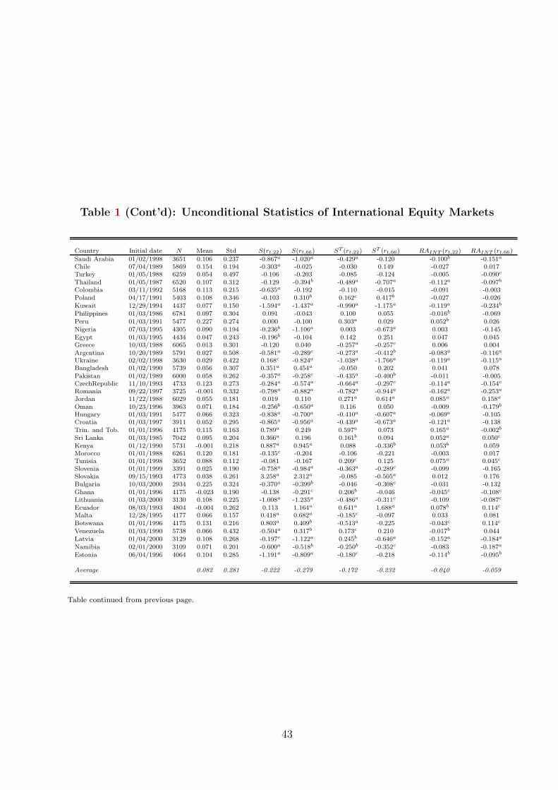
Table 1 (Cont’d): Unconditional Statistics of International Equity Markets

Country Initial date N Mean Std S(rt,22) S(rt,66) ST (rt,22) ST (rt,66) RAINT (rt,22) RAINT (rt,66)

Saudi Arabia 01/02/1998 3651 0.106 0.237 -0.867a -1.020a -0.429a -0.120 -0.100b -0.151a

Chile 07/04/1989 5869 0.154 0.194 -0.303a -0.025 -0.030 0.149 -0.027 0.017Turkey 01/05/1988 6259 0.054 0.497 -0.106 -0.203 -0.085 -0.124 -0.005 -0.090c

Thailand 01/05/1987 6520 0.107 0.312 -0.129 -0.394b -0.489a -0.707a -0.112a -0.097b

Colombia 03/11/1992 5168 0.113 0.215 -0.635a -0.192 -0.110 -0.015 -0.091 -0.003Poland 04/17/1991 5403 0.108 0.346 -0.103 0.310b 0.162c 0.417b -0.027 -0.026Kuwait 12/29/1994 4437 0.077 0.150 -1.594a -1.437a -0.990a -1.175a -0.119a -0.234b

Philippines 01/03/1986 6781 0.097 0.304 0.091 -0.043 0.100 0.055 -0.016b -0.069Peru 01/03/1991 5477 0.227 0.274 0.000 -0.100 0.303a 0.029 0.052b 0.026Nigeria 07/03/1995 4305 0.090 0.194 -0.236b -1.106a 0.003 -0.673a 0.003 -0.145Egypt 01/03/1995 4434 0.047 0.243 -0.196b -0.104 0.142 0.251 0.047 0.045Greece 10/03/1988 6065 0.013 0.301 -0.120 0.040 -0.257a -0.257c 0.006 0.004Argentina 10/20/1989 5791 0.027 0.508 -0.581a -0.289c -0.273a -0.412b -0.083a -0.116a

Ukraine 02/02/1998 3630 0.029 0.422 0.168c -0.824a -1.038a -1.766a -0.119a -0.115a

Bangladesh 01/02/1990 5739 0.056 0.307 0.351a 0.454a -0.050 0.202 0.041 0.078Pakistan 01/02/1989 6000 0.058 0.262 -0.357a -0.258c -0.435a -0.400b -0.011 -0.005CzechRepublic 11/10/1993 4733 0.123 0.273 -0.284a -0.574a -0.664a -0.297c -0.114a -0.154c

Romania 09/22/1997 3725 -0.001 0.332 -0.798a -0.882a -0.782a -0.944a -0.162a -0.253a

Jordan 11/22/1988 6029 0.055 0.181 0.019 0.110 0.271a 0.614a 0.085a 0.158a

Oman 10/23/1996 3963 0.071 0.184 -0.256b -0.650a 0.116 0.050 -0.009 -0.179b

Hungary 01/03/1991 5477 0.066 0.323 -0.838a -0.700a -0.410a -0.607a -0.069a -0.105Croatia 01/03/1997 3911 0.052 0.295 -0.865a -0.956a -0.439a -0.673a -0.121a -0.138Trin. and Tob. 01/01/1996 4175 0.115 0.163 0.789a 0.249 0.597a 0.073 0.165a -0.002b

Sri Lanka 01/03/1985 7042 0.095 0.204 0.366a 0.196 0.161b 0.094 0.052a 0.050c

Kenya 01/12/1990 5731 -0.001 0.218 0.887a 0.945a 0.088 -0.336b 0.053b 0.059Morocco 01/01/1988 6261 0.120 0.181 -0.135c -0.204 -0.106 -0.221 -0.003 0.017Tunisia 01/01/1998 3652 0.088 0.112 -0.081 -0.167 0.209c 0.125 0.075a 0.045c

Slovenia 01/01/1999 3391 0.025 0.190 -0.758a -0.984a -0.363a -0.289c -0.099 -0.165Slovakia 09/15/1993 4773 0.038 0.261 3.258a 2.312a -0.085 -0.505a 0.012 0.176Bulgaria 10/03/2000 2934 0.225 0.324 -0.370a -0.399b -0.046 -0.308c -0.031 -0.132Ghana 01/01/1996 4175 -0.023 0.190 -0.138 -0.291c 0.206b -0.046 -0.045c -0.108c

Lithuania 01/03/2000 3130 0.108 0.225 -1.008a -1.235a -0.486a -0.311c -0.109 -0.087c

Ecuador 08/03/1993 4804 -0.004 0.262 0.113 1.164a 0.641a 1.688a 0.078b 0.114c

Malta 12/28/1995 4177 0.066 0.157 0.418a 0.682a -0.185c -0.097 0.033 0.081Botswana 01/01/1996 4175 0.131 0.216 0.803a 0.409b -0.513a -0.225 -0.043c 0.114c

Venezuela 01/03/1990 5738 0.066 0.432 -0.504a 0.317b 0.173c 0.210 -0.017b 0.044Latvia 01/04/2000 3129 0.108 0.268 -0.197c -1.122a 0.245b -0.646a -0.152a -0.184a

Namibia 02/01/2000 3109 0.071 0.201 -0.600a -0.518b -0.250b -0.352c -0.083 -0.187a

Estonia 06/04/1996 4064 0.104 0.285 -1.191a -0.809a -0.180c -0.218 -0.114b -0.095b

Average 0.082 0.281 -0.222 -0.279 -0.172 -0.232 -0.040 -0.059

Table continued from previous page.

43

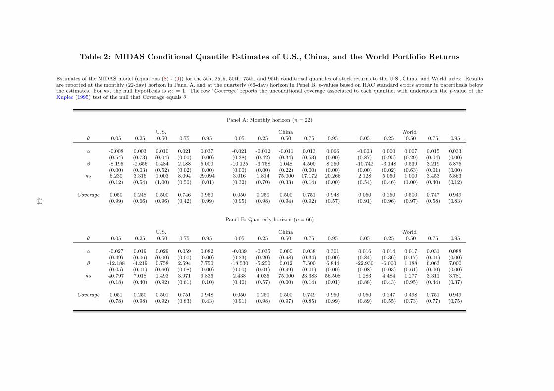
Table 2: MIDAS Conditional Quantile Estimates of U.S., China, and the World Portfolio Returns

Estimates of the MIDAS model (equations (8) - (9)) for the 5th, 25th, 50th, 75th, and 95th conditional quantiles of stock returns to the U.S., China, and World index. Resultsare reported at the monthly (22-day) horizon in Panel A, and at the quarterly (66-day) horizon in Panel B. p-values based on HAC standard errors appear in parenthesis belowthe estimates. For κ2, the null hypothesis is κ2 = 1. The row ‘Coverage’ reports the unconditional coverage associated to each quantile, with underneath the p-value of theKupiec (1995) test of the null that Coverage equals θ.

Panel A: Monthly horizon (n = 22)

U.S. China Worldθ 0.05 0.25 0.50 0.75 0.95 0.05 0.25 0.50 0.75 0.95 0.05 0.25 0.50 0.75 0.95

α -0.008 0.003 0.010 0.021 0.037 -0.021 -0.012 -0.011 0.013 0.066 -0.003 0.000 0.007 0.015 0.033(0.54) (0.73) (0.04) (0.00) (0.00) (0.38) (0.42) (0.34) (0.53) (0.00) (0.87) (0.95) (0.29) (0.04) (0.00)

β -8.195 -2.656 0.484 2.188 5.000 -10.125 -3.758 1.048 4.500 8.250 -10.742 -3.148 0.539 3.219 5.875(0.00) (0.03) (0.52) (0.02) (0.00) (0.00) (0.00) (0.22) (0.00) (0.00) (0.00) (0.02) (0.63) (0.01) (0.00)

κ2 6.230 3.316 1.003 8.094 29.094 3.016 1.814 75.000 17.172 20.266 2.128 5.050 1.000 3.453 5.863(0.12) (0.54) (1.00) (0.50) (0.01) (0.32) (0.70) (0.33) (0.14) (0.00) (0.54) (0.46) (1.00) (0.40) (0.12)

Coverage 0.050 0.248 0.500 0.746 0.950 0.050 0.250 0.500 0.751 0.948 0.050 0.250 0.500 0.747 0.949(0.99) (0.66) (0.96) (0.42) (0.99) (0.95) (0.98) (0.94) (0.92) (0.57) (0.91) (0.96) (0.97) (0.58) (0.83)

Panel B: Quarterly horizon (n = 66)

U.S. China Worldθ 0.05 0.25 0.50 0.75 0.95 0.05 0.25 0.50 0.75 0.95 0.05 0.25 0.50 0.75 0.95

α -0.027 0.019 0.029 0.059 0.082 -0.039 -0.035 0.000 0.038 0.301 0.016 0.014 0.017 0.031 0.088(0.49) (0.06) (0.00) (0.00) (0.00) (0.23) (0.20) (0.98) (0.34) (0.00) (0.84) (0.36) (0.17) (0.01) (0.00)

β -12.188 -4.219 0.758 2.594 7.750 -18.530 -5.250 0.012 7.500 6.844 -22.930 -6.000 1.188 6.063 7.000(0.05) (0.01) (0.60) (0.08) (0.00) (0.00) (0.01) (0.99) (0.01) (0.00) (0.08) (0.03) (0.61) (0.00) (0.00)

κ2 40.797 7.018 1.493 3.971 9.836 2.438 4.035 75.000 23.383 56.508 1.283 4.484 1.277 3.311 3.781(0.18) (0.40) (0.92) (0.61) (0.10) (0.40) (0.57) (0.00) (0.14) (0.01) (0.88) (0.43) (0.95) (0.44) (0.37)

Coverage 0.051 0.250 0.501 0.751 0.948 0.050 0.250 0.500 0.749 0.950 0.050 0.247 0.498 0.751 0.949(0.78) (0.98) (0.92) (0.83) (0.43) (0.91) (0.98) (0.97) (0.85) (0.99) (0.89) (0.55) (0.73) (0.77) (0.75)

44

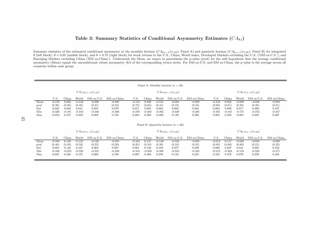
Table 3: Summary Statistics of Conditional Asymmetry Estimates (CAθ,t)

Summary statistics of the estimated conditional asymmetry at the monthly horizon (CAθ,t−1(rt,22), Panel A) and quarterly horizon (CAθ,t−1(rt,66), Panel B) for integratedθ (left block), θ = 0.95 (middle block), and θ = 0.75 (right block) for stock returns to the U.S., China, World index, Developed Markets excluding the U.S. (‘DM ex-U.S.’), andEmerging Markets excluding China (‘EM ex-China’). Underneath the Mean, we report in parenthesis the p-value (pval) for the null hypothesis that the average conditionalasymmetry (Mean) equals the unconditional robust asymmetry RA of the corresponding return series. For DM ex-U.S. and EM ex-China, the p-value is the average across allcountries within each group.

Panel A: Monthly horizon (n = 22)

CAINT,t−1(rt,22) CA0.95,t−1(rt,22) CA0.75,t−1(rt,22)

U.S. China World DM ex-U.S. EM ex-China U.S. China World DM ex-U.S. EM ex-China U.S. China World DM ex-U.S. EM ex-ChinaMean -0.159 0.063 -0.142 -0.098 -0.028 -0.145 0.038 -0.131 -0.084 -0.029 -0.124 0.023 -0.098 -0.039 -0.003pval (0.39) (0.36) (0.40) (0.21) (0.16) (0.75) (0.63) (0.44) (0.19) (0.16) (0.00) (0.81) (0.20) (0.28) (0.21)Std 0.048 0.084 0.041 0.055 0.079 0.071 0.095 0.062 0.063 0.083 0.064 0.098 0.017 0.089 0.107Min -0.320 -0.191 -0.310 -0.346 -0.306 -0.370 -0.303 -0.362 -0.330 -0.305 -0.401 -0.445 -0.175 -0.372 -0.347Max -0.052 0.275 -0.055 0.069 0.195 0.204 0.268 -0.009 0.120 0.206 0.063 0.288 -0.061 0.205 0.307

Panel B: Quarterly horizon (n = 66)

CAINT,t−1(rt,66) CA0.95,t−1(rt,66) CA0.75,t−1(rt,66)

U.S. China World DM ex-U.S. EM ex-China U.S. China World DM ex-U.S. EM ex-China U.S. China World DM ex-U.S. EM ex-ChinaMean -0.168 0.128 -0.125 -0.120 -0.055 -0.163 0.147 -0.140 -0.102 -0.035 -0.013 0.117 -0.028 -0.035 -0.020pval (0.40) (0.10) (0.58) (0.23) (0.20) (0.25) (0.10) (0.30) (0.18) (0.25) (0.83) (0.00) (0.89) (0.21) (0.23)Std 0.083 0.120 0.127 0.062 0.087 0.061 0.136 0.108 0.077 0.099 0.088 0.097 0.041 0.095 0.163Min -0.436 -0.253 -0.526 -0.325 -0.320 -0.444 -0.269 -0.496 -0.324 -0.335 -0.312 -0.303 -0.143 -0.325 -0.471Max 0.002 0.426 0.155 0.069 0.196 0.007 0.466 0.199 0.144 0.245 0.165 0.476 0.079 0.239 0.456

45

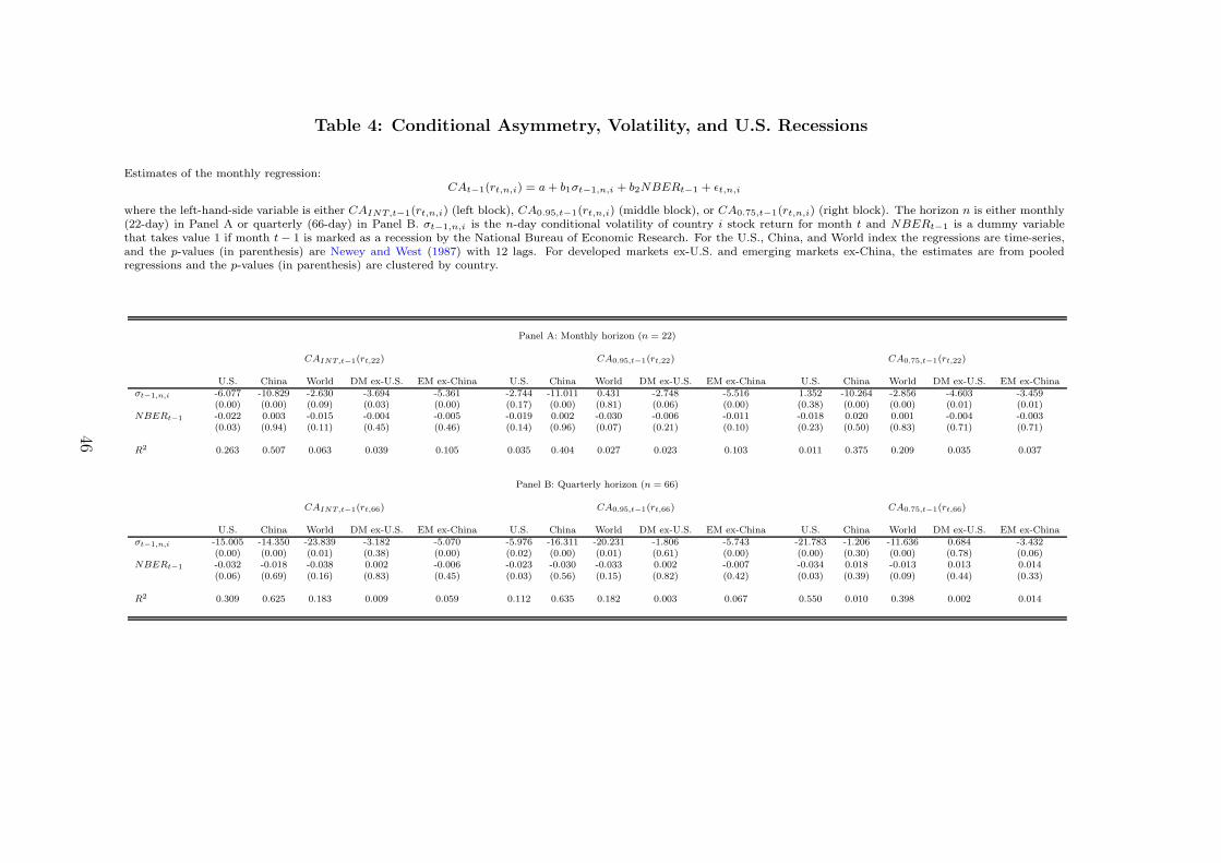
Table 4: Conditional Asymmetry, Volatility, and U.S. Recessions

Estimates of the monthly regression:CAt−1(rt,n,i) = a+ b1σt−1,n,i + b2NBERt−1 + ǫt,n,i

where the left-hand-side variable is either CAINT,t−1(rt,n,i) (left block), CA0.95,t−1(rt,n,i) (middle block), or CA0.75,t−1(rt,n,i) (right block). The horizon n is either monthly(22-day) in Panel A or quarterly (66-day) in Panel B. σt−1,n,i is the n-day conditional volatility of country i stock return for month t and NBERt−1 is a dummy variablethat takes value 1 if month t− 1 is marked as a recession by the National Bureau of Economic Research. For the U.S., China, and World index the regressions are time-series,and the p-values (in parenthesis) are Newey and West (1987) with 12 lags. For developed markets ex-U.S. and emerging markets ex-China, the estimates are from pooledregressions and the p-values (in parenthesis) are clustered by country.

Panel A: Monthly horizon (n = 22)

CAINT,t−1(rt,22) CA0.95,t−1(rt,22) CA0.75,t−1(rt,22)

U.S. China World DM ex-U.S. EM ex-China U.S. China World DM ex-U.S. EM ex-China U.S. China World DM ex-U.S. EM ex-Chinaσt−1,n,i -6.077 -10.829 -2.630 -3.694 -5.361 -2.744 -11.011 0.431 -2.748 -5.516 1.352 -10.264 -2.856 -4.603 -3.459

(0.00) (0.00) (0.09) (0.03) (0.00) (0.17) (0.00) (0.81) (0.06) (0.00) (0.38) (0.00) (0.00) (0.01) (0.01)NBERt−1 -0.022 0.003 -0.015 -0.004 -0.005 -0.019 0.002 -0.030 -0.006 -0.011 -0.018 0.020 0.001 -0.004 -0.003

(0.03) (0.94) (0.11) (0.45) (0.46) (0.14) (0.96) (0.07) (0.21) (0.10) (0.23) (0.50) (0.83) (0.71) (0.71)

R2 0.263 0.507 0.063 0.039 0.105 0.035 0.404 0.027 0.023 0.103 0.011 0.375 0.209 0.035 0.037

Panel B: Quarterly horizon (n = 66)

CAINT,t−1(rt,66) CA0.95,t−1(rt,66) CA0.75,t−1(rt,66)

U.S. China World DM ex-U.S. EM ex-China U.S. China World DM ex-U.S. EM ex-China U.S. China World DM ex-U.S. EM ex-Chinaσt−1,n,i -15.005 -14.350 -23.839 -3.182 -5.070 -5.976 -16.311 -20.231 -1.806 -5.743 -21.783 -1.206 -11.636 0.684 -3.432

(0.00) (0.00) (0.01) (0.38) (0.00) (0.02) (0.00) (0.01) (0.61) (0.00) (0.00) (0.30) (0.00) (0.78) (0.06)NBERt−1 -0.032 -0.018 -0.038 0.002 -0.006 -0.023 -0.030 -0.033 0.002 -0.007 -0.034 0.018 -0.013 0.013 0.014

(0.06) (0.69) (0.16) (0.83) (0.45) (0.03) (0.56) (0.15) (0.82) (0.42) (0.03) (0.39) (0.09) (0.44) (0.33)

R2 0.309 0.625 0.183 0.009 0.059 0.112 0.635 0.182 0.003 0.067 0.550 0.010 0.398 0.002 0.014

46

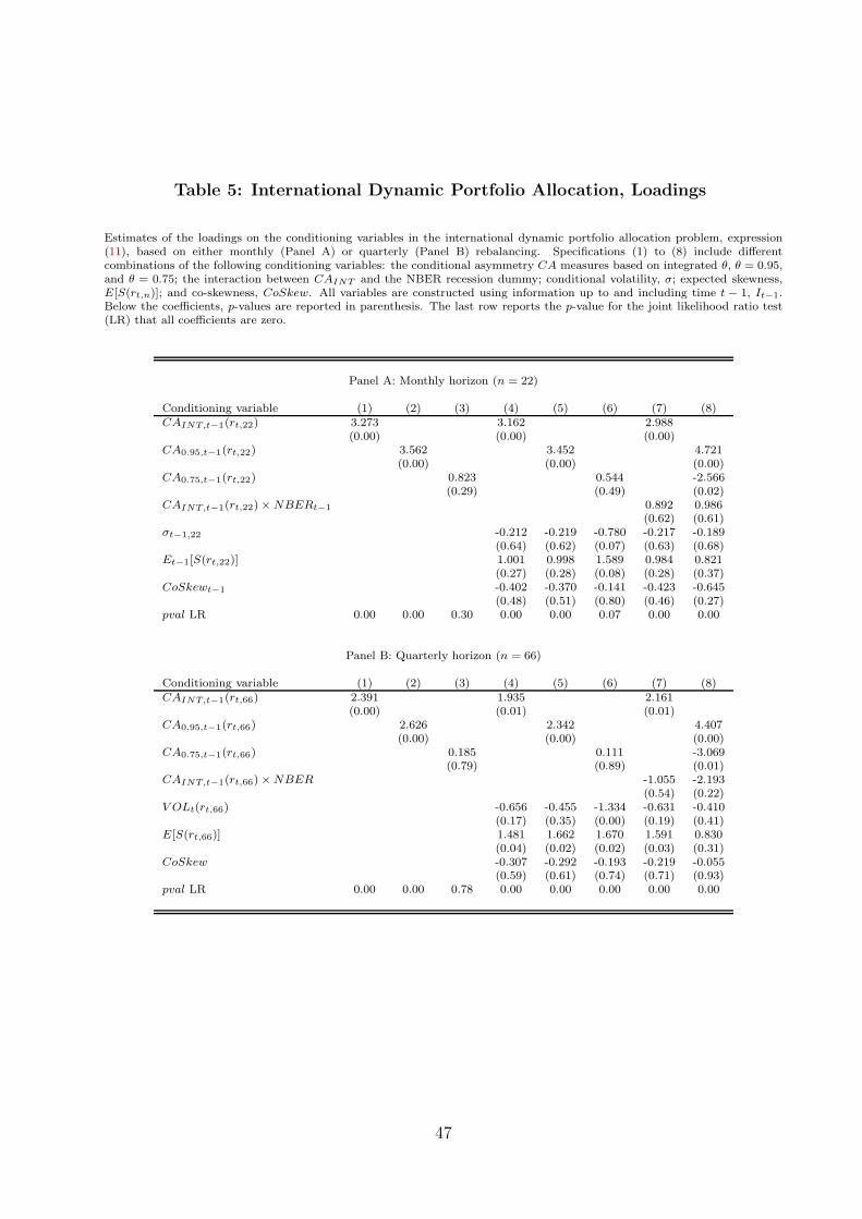
Table 5: International Dynamic Portfolio Allocation, Loadings

Estimates of the loadings on the conditioning variables in the international dynamic portfolio allocation problem, expression(11), based on either monthly (Panel A) or quarterly (Panel B) rebalancing. Specifications (1) to (8) include differentcombinations of the following conditioning variables: the conditional asymmetry CA measures based on integrated θ, θ = 0.95,and θ = 0.75; the interaction between CAINT and the NBER recession dummy; conditional volatility, σ; expected skewness,E[S(rt,n)]; and co-skewness, CoSkew. All variables are constructed using information up to and including time t − 1, It−1.Below the coefficients, p-values are reported in parenthesis. The last row reports the p-value for the joint likelihood ratio test(LR) that all coefficients are zero.

Panel A: Monthly horizon (n = 22)

Conditioning variable (1) (2) (3) (4) (5) (6) (7) (8)CAINT,t−1(rt,22) 3.273 3.162 2.988

(0.00) (0.00) (0.00)CA0.95,t−1(rt,22) 3.562 3.452 4.721

(0.00) (0.00) (0.00)CA0.75,t−1(rt,22) 0.823 0.544 -2.566

(0.29) (0.49) (0.02)CAINT,t−1(rt,22)×NBERt−1 0.892 0.986

(0.62) (0.61)σt−1,22 -0.212 -0.219 -0.780 -0.217 -0.189

(0.64) (0.62) (0.07) (0.63) (0.68)Et−1[S(rt,22)] 1.001 0.998 1.589 0.984 0.821

(0.27) (0.28) (0.08) (0.28) (0.37)CoSkewt−1 -0.402 -0.370 -0.141 -0.423 -0.645

(0.48) (0.51) (0.80) (0.46) (0.27)pval LR 0.00 0.00 0.30 0.00 0.00 0.07 0.00 0.00

Panel B: Quarterly horizon (n = 66)

Conditioning variable (1) (2) (3) (4) (5) (6) (7) (8)CAINT,t−1(rt,66) 2.391 1.935 2.161

(0.00) (0.01) (0.01)CA0.95,t−1(rt,66) 2.626 2.342 4.407

(0.00) (0.00) (0.00)CA0.75,t−1(rt,66) 0.185 0.111 -3.069

(0.79) (0.89) (0.01)CAINT,t−1(rt,66)×NBER -1.055 -2.193

(0.54) (0.22)V OLt(rt,66) -0.656 -0.455 -1.334 -0.631 -0.410

(0.17) (0.35) (0.00) (0.19) (0.41)E[S(rt,66)] 1.481 1.662 1.670 1.591 0.830

(0.04) (0.02) (0.02) (0.03) (0.31)CoSkew -0.307 -0.292 -0.193 -0.219 -0.055

(0.59) (0.61) (0.74) (0.71) (0.93)pval LR 0.00 0.00 0.78 0.00 0.00 0.00 0.00 0.00

47

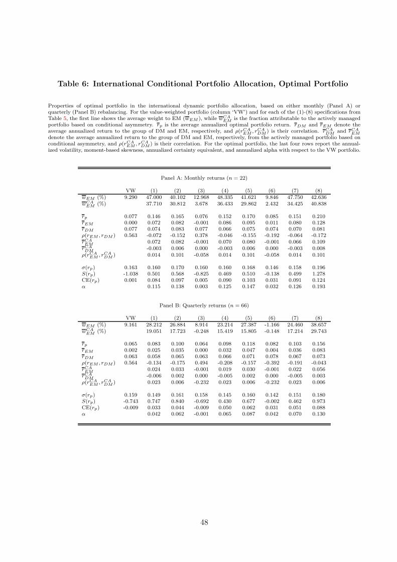
Table 6: International Conditional Portfolio Allocation, Optimal Portfolio

Properties of optimal portfolio in the international dynamic portfolio allocation, based on either monthly (Panel A) orquarterly (Panel B) rebalancing. For the value-weighted portfolio (column ‘VW’) and for each of the (1)-(8) specifications fromTable 5, the first line shows the average weight to EM (wEM ), while wCA

EMis the fraction attributable to the actively managed

portfolio based on conditional asymmetry. rp is the average annualized optimal portfolio return. rDM and rEM denote theaverage annualized return to the group of DM and EM, respectively, and ρ(rCA

EM, rCA

DM) is their correlation. rCA

DMand rCA

EMdenote the average annualized return to the group of DM and EM, respectively, from the actively managed portfolio based onconditional asymmetry, and ρ(rCA

EM , rCADM) is their correlation. For the optimal portfolio, the last four rows report the annual-

ized volatility, moment-based skewness, annualized certainty equivalent, and annualized alpha with respect to the VW portfolio.

Panel A: Monthly returns (n = 22)

VW (1) (2) (3) (4) (5) (6) (7) (8)wEM (%) 9.290 47.000 40.102 12.968 48.335 41.621 9.846 47.750 42.636wCA

EM (%) 37.710 30.812 3.678 36.433 29.862 2.432 34.425 40.838

rp 0.077 0.146 0.165 0.076 0.152 0.170 0.085 0.151 0.210rEM 0.000 0.072 0.082 -0.001 0.086 0.095 0.011 0.080 0.128rDM 0.077 0.074 0.083 0.077 0.066 0.075 0.074 0.070 0.081ρ(rEM , rDM ) 0.563 -0.072 -0.152 0.378 -0.046 -0.155 -0.192 -0.064 -0.172rCAEM

0.072 0.082 -0.001 0.070 0.080 -0.001 0.066 0.109rCADM

-0.003 0.006 0.000 -0.003 0.006 0.000 -0.003 0.008ρ(rCA

EM , rCADM ) 0.014 0.101 -0.058 0.014 0.101 -0.058 0.014 0.101

σ(rp) 0.163 0.160 0.170 0.160 0.160 0.168 0.146 0.158 0.196S(rp) -1.038 0.501 0.568 -0.825 0.469 0.510 -0.138 0.499 1.278CE(rp) 0.001 0.084 0.097 0.005 0.090 0.103 0.031 0.091 0.124α 0.115 0.138 0.003 0.125 0.147 0.032 0.126 0.193

Panel B: Quarterly returns (n = 66)

VW (1) (2) (3) (4) (5) (6) (7) (8)wEM (%) 9.161 28.212 26.884 8.914 23.214 27.387 -1.166 24.460 38.657wCA

EM (%) 19.051 17.723 -0.248 15.419 15.805 -0.148 17.214 29.743

rp 0.065 0.083 0.100 0.064 0.098 0.118 0.082 0.103 0.156rEM 0.002 0.025 0.035 0.000 0.032 0.047 0.004 0.036 0.083rDM 0.063 0.058 0.065 0.063 0.066 0.071 0.078 0.067 0.073ρ(rEM , rDM ) 0.564 -0.134 -0.175 0.494 -0.208 -0.157 -0.392 -0.191 -0.043rCAEM

0.024 0.033 -0.001 0.019 0.030 -0.001 0.022 0.056rCADM

-0.006 0.002 0.000 -0.005 0.002 0.000 -0.005 0.003ρ(rCA

EM, rCA

DM) 0.023 0.006 -0.232 0.023 0.006 -0.232 0.023 0.006

σ(rp) 0.159 0.149 0.161 0.158 0.145 0.160 0.142 0.151 0.180S(rp) -0.743 0.747 0.840 -0.692 0.430 0.677 -0.002 0.462 0.973CE(rp) -0.009 0.033 0.044 -0.009 0.050 0.062 0.031 0.051 0.088α 0.042 0.062 -0.001 0.065 0.087 0.042 0.070 0.130

48

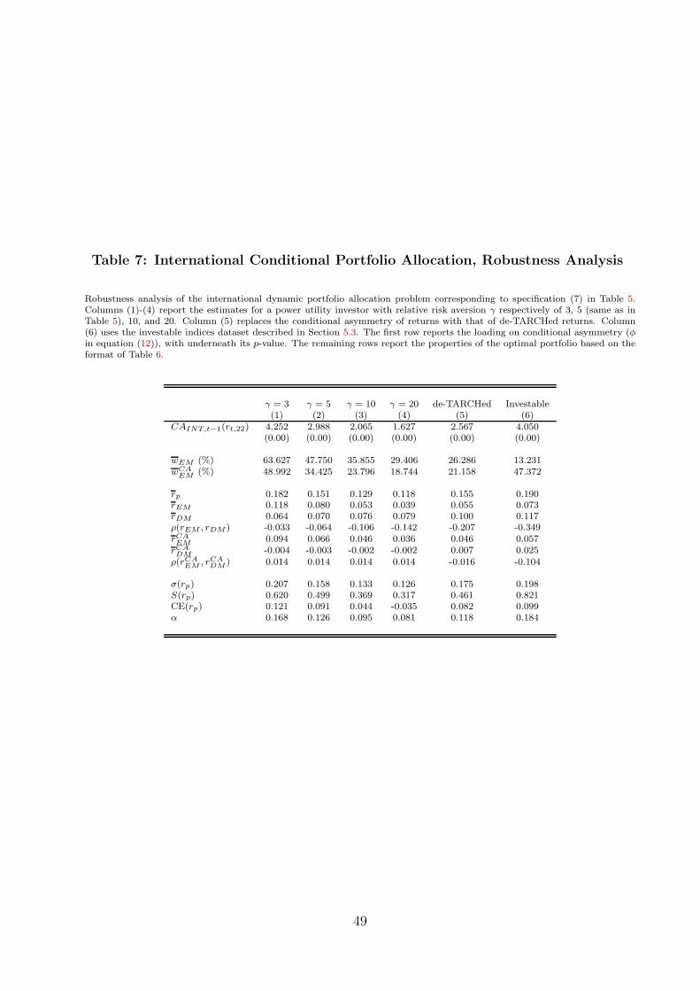
Table 7: International Conditional Portfolio Allocation, Robustness Analysis

Robustness analysis of the international dynamic portfolio allocation problem corresponding to specification (7) in Table 5.Columns (1)-(4) report the estimates for a power utility investor with relative risk aversion γ respectively of 3, 5 (same as inTable 5), 10, and 20. Column (5) replaces the conditional asymmetry of returns with that of de-TARCHed returns. Column(6) uses the investable indices dataset described in Section 5.3. The first row reports the loading on conditional asymmetry (φin equation (12)), with underneath its p-value. The remaining rows report the properties of the optimal portfolio based on theformat of Table 6.

γ = 3 γ = 5 γ = 10 γ = 20 de-TARCHed Investable(1) (2) (3) (4) (5) (6)

CAINT,t−1(rt,22) 4.252 2.988 2.065 1.627 2.567 4.050(0.00) (0.00) (0.00) (0.00) (0.00) (0.00)

wEM (%) 63.627 47.750 35.855 29.406 26.286 13.231wCA

EM (%) 48.992 34.425 23.796 18.744 21.158 47.372

rp 0.182 0.151 0.129 0.118 0.155 0.190rEM 0.118 0.080 0.053 0.039 0.055 0.073rDM 0.064 0.070 0.076 0.079 0.100 0.117ρ(rEM , rDM) -0.033 -0.064 -0.106 -0.142 -0.207 -0.349rCAEM

0.094 0.066 0.046 0.036 0.046 0.057rCADM

-0.004 -0.003 -0.002 -0.002 0.007 0.025ρ(rCA

EM , rCADM) 0.014 0.014 0.014 0.014 -0.016 -0.104

σ(rp) 0.207 0.158 0.133 0.126 0.175 0.198S(rp) 0.620 0.499 0.369 0.317 0.461 0.821CE(rp) 0.121 0.091 0.044 -0.035 0.082 0.099α 0.168 0.126 0.095 0.081 0.118 0.184

49

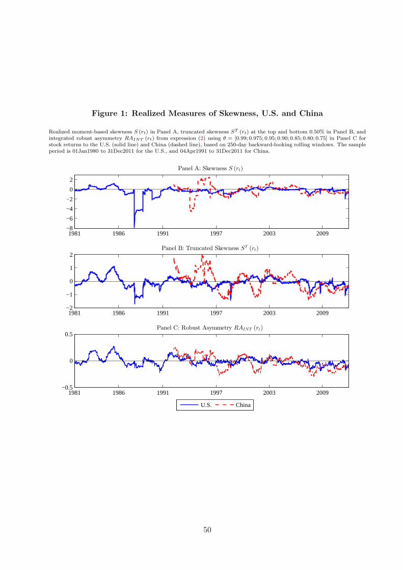
Figure 1: Realized Measures of Skewness, U.S. and China

Realized moment-based skewness S (rt) in Panel A, truncated skewness ST (rt) at the top and bottom 0.50% in Panel B, andintegrated robust asymmetry RAINT (rt) from expression (2) using θ = [0.99; 0.975; 0.95; 0.90; 0.85; 0.80; 0.75] in Panel C forstock returns to the U.S. (solid line) and China (dashed line), based on 250-day backward-looking rolling windows. The sampleperiod is 01Jan1980 to 31Dec2011 for the U.S., and 04Apr1991 to 31Dec2011 for China.

1981 1986 1991 1997 2003 2009−8

−6

−4

−2

0

2

Panel A: Skewness S (rt)

1981 1986 1991 1997 2003 2009−2

−1

0

1

2Panel B: Truncated Skewness ST (rt)

1981 1986 1991 1997 2003 2009−0.5

0

0.5Panel C: Robust Asymmetry RAINT (rt)

U.S. China

50

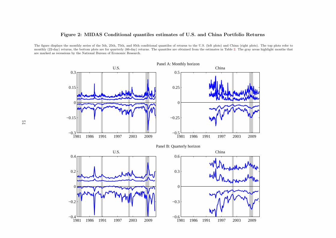
Figure 2: MIDAS Conditional quantiles estimates of U.S. and China Portfolio Returns

The figure displays the monthly series of the 5th, 25th, 75th, and 95th conditional quantiles of returns to the U.S. (left plots) and China (right plots). The top plots refer tomonthly (22-day) returns, the bottom plots are for quarterly (66-day) returns. The quantiles are obtained from the estimates in Table 2. The gray areas highlight months thatare marked as recessions by the National Bureau of Economic Research.

U.S.

1981 1986 1991 1997 2003 2009−0.3

−0.15

0

0.15

0.3China

Panel A: Monthly horizon

1981 1986 1991 1997 2003 2009−0.5

−0.25

0

0.25

0.5

U.S.

1981 1986 1991 1997 2003 2009−0.4

−0.2

0

0.2

0.4China

Panel B: Quarterly horizon

1981 1986 1991 1997 2003 2009−0.6

−0.3

0

0.3

0.6

51

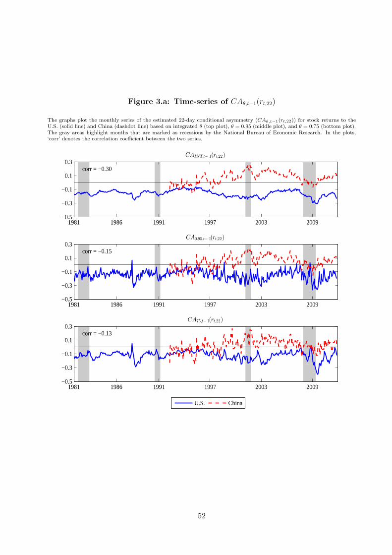
Figure 3.a: Time-series of CAθ,t−1(rt,22)

The graphs plot the monthly series of the estimated 22-day conditional asymmetry (CAθ,t−1(rt,22)) for stock returns to theU.S. (solid line) and China (dashdot line) based on integrated θ (top plot), θ = 0.95 (middle plot), and θ = 0.75 (bottom plot).The gray areas highlight months that are marked as recessions by the National Bureau of Economic Research. In the plots,‘corr’ denotes the correlation coefficient between the two series.

CA0.95,t− 1(rt,22)

corr = −0.15

1981 1986 1991 1997 2003 2009−0.5

−0.3

−0.1

0.1

0.3

CA75,t− 1(rt,22)

corr = −0.13

1981 1986 1991 1997 2003 2009−0.5

−0.3

−0.1

0.1

0.3

U.S. China

CAINT,t− 1(rt,22)

corr = −0.30

1981 1986 1991 1997 2003 2009−0.5

−0.3

−0.1

0.1

0.3

52

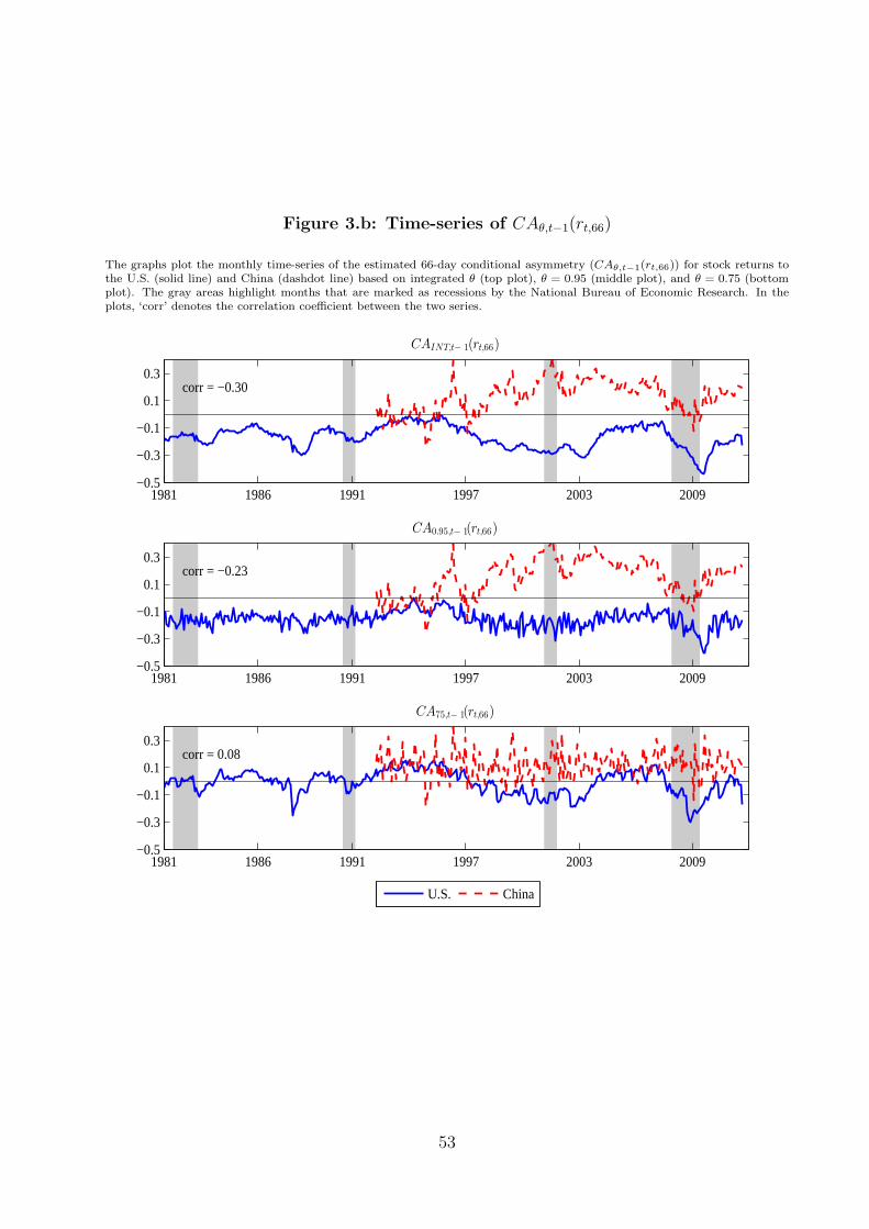
Figure 3.b: Time-series of CAθ,t−1(rt,66)

The graphs plot the monthly time-series of the estimated 66-day conditional asymmetry (CAθ,t−1(rt,66)) for stock returns tothe U.S. (solid line) and China (dashdot line) based on integrated θ (top plot), θ = 0.95 (middle plot), and θ = 0.75 (bottomplot). The gray areas highlight months that are marked as recessions by the National Bureau of Economic Research. In theplots, ‘corr’ denotes the correlation coefficient between the two series.

CA0.95,t− 1(rt,66)

corr = −0.23

1981 1986 1991 1997 2003 2009−0.5

−0.3

−0.1

0.1

0.3

CA75,t− 1(rt,66)

corr = 0.08

1981 1986 1991 1997 2003 2009−0.5

−0.3

−0.1

0.1

0.3

U.S. China

CAINT,t− 1(rt,66)

corr = −0.30

1981 1986 1991 1997 2003 2009−0.5

−0.3

−0.1

0.1

0.3

53

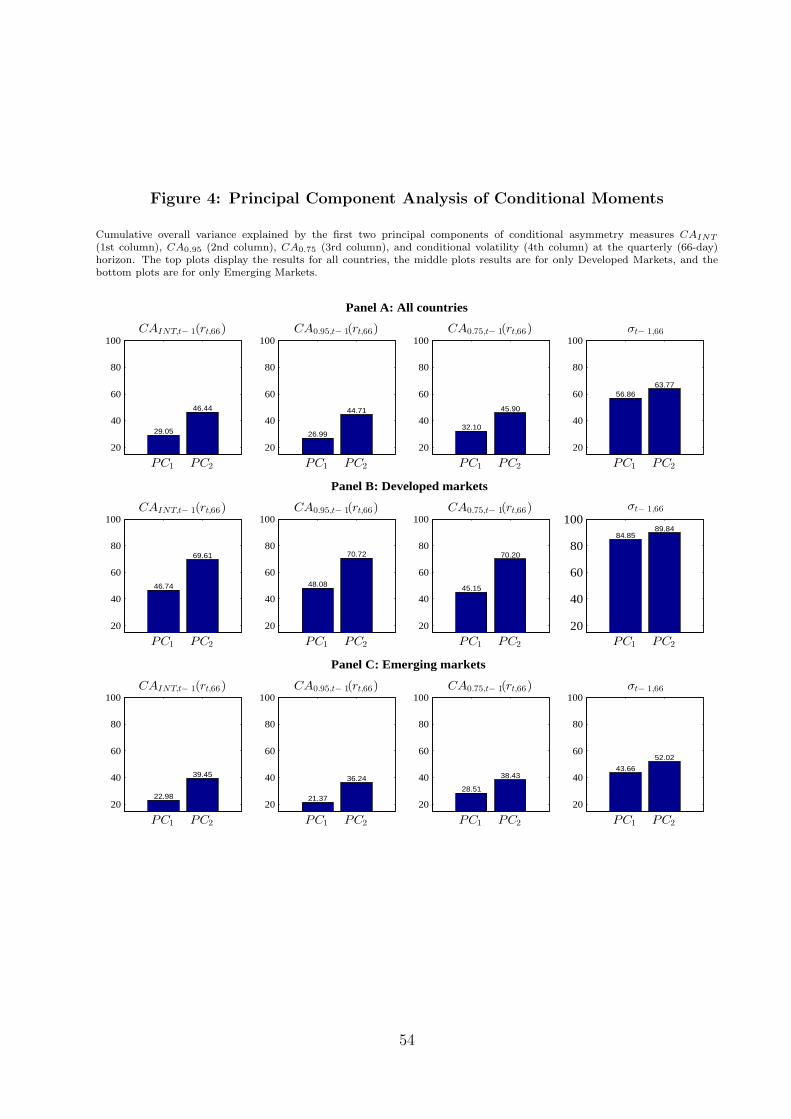
Figure 4: Principal Component Analysis of Conditional Moments

Cumulative overall variance explained by the first two principal components of conditional asymmetry measures CAINT

(1st column), CA0.95 (2nd column), CA0.75 (3rd column), and conditional volatility (4th column) at the quarterly (66-day)horizon. The top plots display the results for all countries, the middle plots results are for only Developed Markets, and thebottom plots are for only Emerging Markets.

20

40

60

80

100

29.05

46.44

CAINT,t− 1(rt,66)

PC1 PC2

20

40

60

80

100

26.99

44.71

CA0.95,t− 1(rt,66)

PC1 PC2

20

40

60

80

100

32.10

45.90

CA0.75,t− 1(rt,66)

PC1 PC2

20

40

60

80

100

56.8663.77

σt− 1,66

PC1 PC2

Panel A: All countries

20

40

60

80

100

46.74

69.61

CAINT,t− 1(rt,66)

PC1 PC2

20

40

60

80

100

48.08

70.72

CA0.95,t− 1(rt,66)

PC1 PC2

20

40

60

80

100

45.15

70.20

CA0.75,t− 1(rt,66)

PC1 PC2

20

40

60

80

10084.85

89.84

σt− 1,66

PC1 PC2

Panel B: Developed markets

20

40

60

80

100

22.98

39.45

CAINT,t− 1(rt,66)

PC1 PC2

20

40

60

80

100

21.37

36.24

CA0.95,t− 1(rt,66)

PC1 PC2

20

40

60

80

100

28.51

38.43

CA0.75,t− 1(rt,66)

PC1 PC2

20

40

60

80

100

43.66

52.02

σt− 1,66

PC1 PC2

Panel C: Emerging markets

54

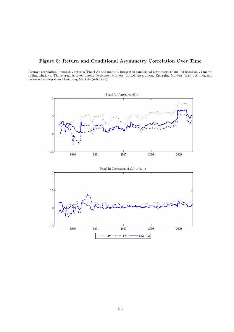
Figure 5: Return and Conditional Asymmetry Correlation Over Time

Average correlation in monthly returns (Panel A) and monthly integrated conditional asymmetry (Panel B) based on 24-monthrolling windows. The average is taken among Developed Markets (dotted line), among Emerging Markets (dash-dot line), andbetween Developed and Emerging Markets (solid line).

1986 1991 1997 2003 2009−0.5

0

0.5

1Panel A: Correlation of rt,22

1986 1991 1997 2003 2009−0.5

0

0.5

1Panel B: Correlation of CAINT (rt,22)

DM EM DM−EM

55

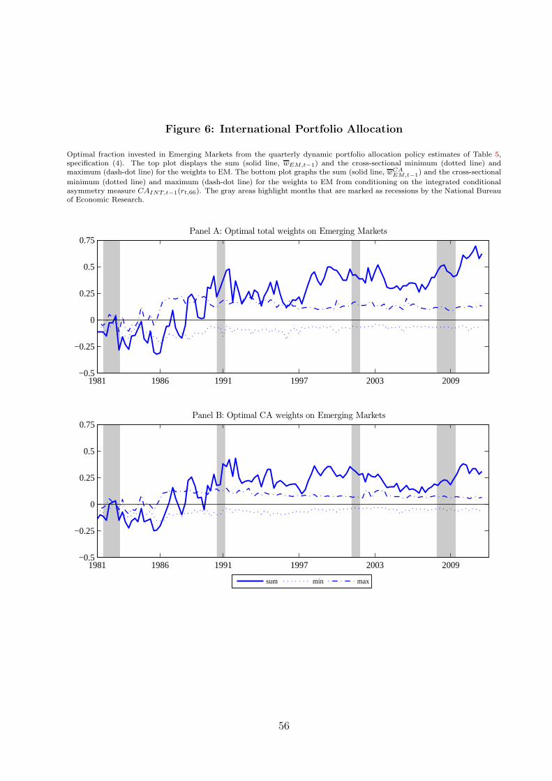
Figure 6: International Portfolio Allocation

Optimal fraction invested in Emerging Markets from the quarterly dynamic portfolio allocation policy estimates of Table 5,specification (4). The top plot displays the sum (solid line, wEM,t−1) and the cross-sectional minimum (dotted line) andmaximum (dash-dot line) for the weights to EM. The bottom plot graphs the sum (solid line, wCA

EM,t−1) and the cross-sectional

minimum (dotted line) and maximum (dash-dot line) for the weights to EM from conditioning on the integrated conditionalasymmetry measure CAINT,t−1(rt,66). The gray areas highlight months that are marked as recessions by the National Bureauof Economic Research.

Panel A: Optimal total weights on Emerging Markets

1981 1986 1991 1997 2003 2009−0.5

−0.25

0

0.25

0.5

0.75

Panel B: Optimal CA weights on Emerging Markets

1981 1986 1991 1997 2003 2009−0.5

−0.25

0

0.25

0.5

0.75

sum min max

56

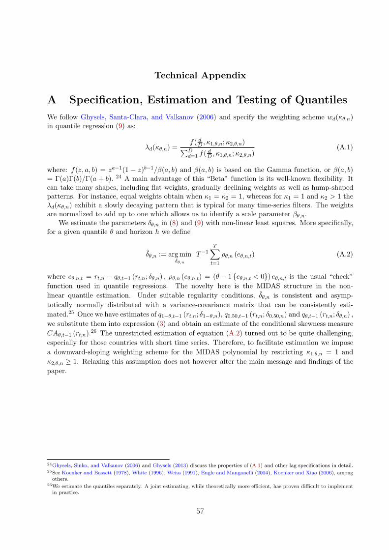
Technical Appendix

A Specification, Estimation and Testing of Quantiles

We follow Ghysels, Santa-Clara, and Valkanov (2006) and specify the weighting scheme wd(κθ,n)in quantile regression (9) as:

λd(κθ,n) =f( d

D , κ1,θ,n;κ2,θ,n)∑Dd=1 f(

dD , κ1,θ,n;κ2,θ,n)

(A.1)

where: f(z, a, b) = za−1(1 − z)b−1/β(a, b) and β(a, b) is based on the Gamma function, or β(a, b)= Γ(a)Γ(b)/Γ(a + b). 24 A main advantage of this “Beta” function is its well-known flexibility. Itcan take many shapes, including flat weights, gradually declining weights as well as hump-shapedpatterns. For instance, equal weights obtain when κ1 = κ2 = 1, whereas for κ1 = 1 and κ2 > 1 theλd(κθ,n) exhibit a slowly decaying pattern that is typical for many time-series filters. The weightsare normalized to add up to one which allows us to identify a scale parameter βθ,n.

We estimate the parameters δθ,n in (8) and (9) with non-linear least squares. More specifically,for a given quantile θ and horizon h we define

δθ,n := argminδθ,n

T−1T∑

t=1

ρθ,n (eθ,n,t) (A.2)

where eθ,n,t = rt,n − qθ,t−1 (rt,n; δθ,n) , ρθ,n (eθ,n,t) = (θ − 1 {eθ,n,t < 0}) eθ,n,t is the usual “check”

function used in quantile regressions. The novelty here is the MIDAS structure in the non-

linear quantile estimation. Under suitable regularity conditions, δθ,n is consistent and asymp-

totically normally distributed with a variance-covariance matrix that can be consistently esti-

mated.25 Once we have estimates of q1−θ,t−1 (rt,n; δ1−θ,n), q0.50,t−1 (rt,n; δ0.50,n) and qθ,t−1 (rt,n; δθ,n) ,

we substitute them into expression (3) and obtain an estimate of the conditional skewness measure

CAθ,t−1 (rt,n).26 The unrestricted estimation of equation (A.2) turned out to be quite challenging,

especially for those countries with short time series. Therefore, to facilitate estimation we impose

a downward-sloping weighting scheme for the MIDAS polynomial by restricting κ1,θ,n = 1 and

κ2,θ,n ≥ 1. Relaxing this assumption does not however alter the main message and findings of the

paper.

24Ghysels, Sinko, and Valkanov (2006) and Ghysels (2013) discuss the properties of (A.1) and other lag specifications in detail.25See Koenker and Bassett (1978), White (1996), Weiss (1991), Engle and Manganelli (2004), Koenker and Xiao (2006), amongothers.

26We estimate the quantiles separately. A joint estimating, while theoretically more efficient, has proven difficult to implementin practice.

57

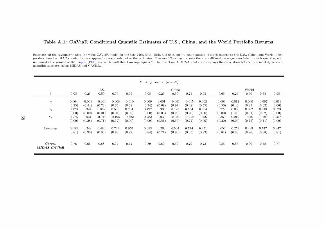
Table A.1: CAViaR Conditional Quantile Estimates of U.S., China, and the World Portfolio Returns

Estimates of the asymmetric absolute value CAViaR model for the 5th, 25th, 50th, 75th, and 95th conditional quantiles of stock returns to the U.S., China, and World index.p-values based on HAC standard errors appear in parenthesis below the estimates. The row ‘Coverage’ reports the unconditional coverage associated to each quantile, withunderneath the p-value of the Kupiec (1995) test of the null that Coverage equals θ. The row ‘Correl. MIDAS-CAViaR’ displays the correlation between the monthly series ofquantiles estimates using MIDAS and CAViaR.

Monthly horizon (n = 22)

U.S. China Worldθ 0.05 0.25 0.50 0.75 0.95 0.05 0.25 0.50 0.75 0.95 0.05 0.25 0.50 0.75 0.95

γ0 0.004 -0.001 -0.001 -0.008 -0.010 0.009 0.001 -0.001 -0.015 0.002 0.003 0.012 0.000 -0.007 -0.013(0.25) (0.44) (0.78) (0.34) (0.08) (0.24) (0.69) (0.94) (0.48) (0.55) (0.50) (0.46) (0.81) (0.32) (0.06)

γ1 0.779 0.944 0.892 0.590 0.704 0.797 0.933 0.125 0.534 0.904 0.772 0.000 0.882 0.618 0.629(0.00) (0.00) (0.01) (0.04) (0.00) (0.00) (0.00) (0.93) (0.20) (0.00) (0.00) (1.00) (0.01) (0.02) (0.00)

γ2 0.276 0.041 -0.017 -0.195 -0.322 0.282 0.039 -0.081 -0.219 -0.222 0.369 0.219 -0.021 -0.190 -0.416(0.00) (0.28) (0.71) (0.12) (0.00) (0.00) (0.51) (0.66) (0.22) (0.00) (0.20) (0.06) (0.75) (0.11) (0.00)

Coverage 0.053 0.248 0.496 0.749 0.950 0.053 0.260 0.504 0.744 0.951 0.053 0.253 0.499 0.747 0.947(0.81) (0.93) (0.88) (0.98) (0.99) (0.84) (0.71) (0.90) (0.83) (0.93) (0.81) (0.88) (0.96) (0.88) (0.81)

Correl. 0.76 0.66 0.88 0.74 0.64 0.89 0.89 0.59 0.79 0.73 0.85 0.53 0.90 0.78 0.77MIDAS-CAViaR

58

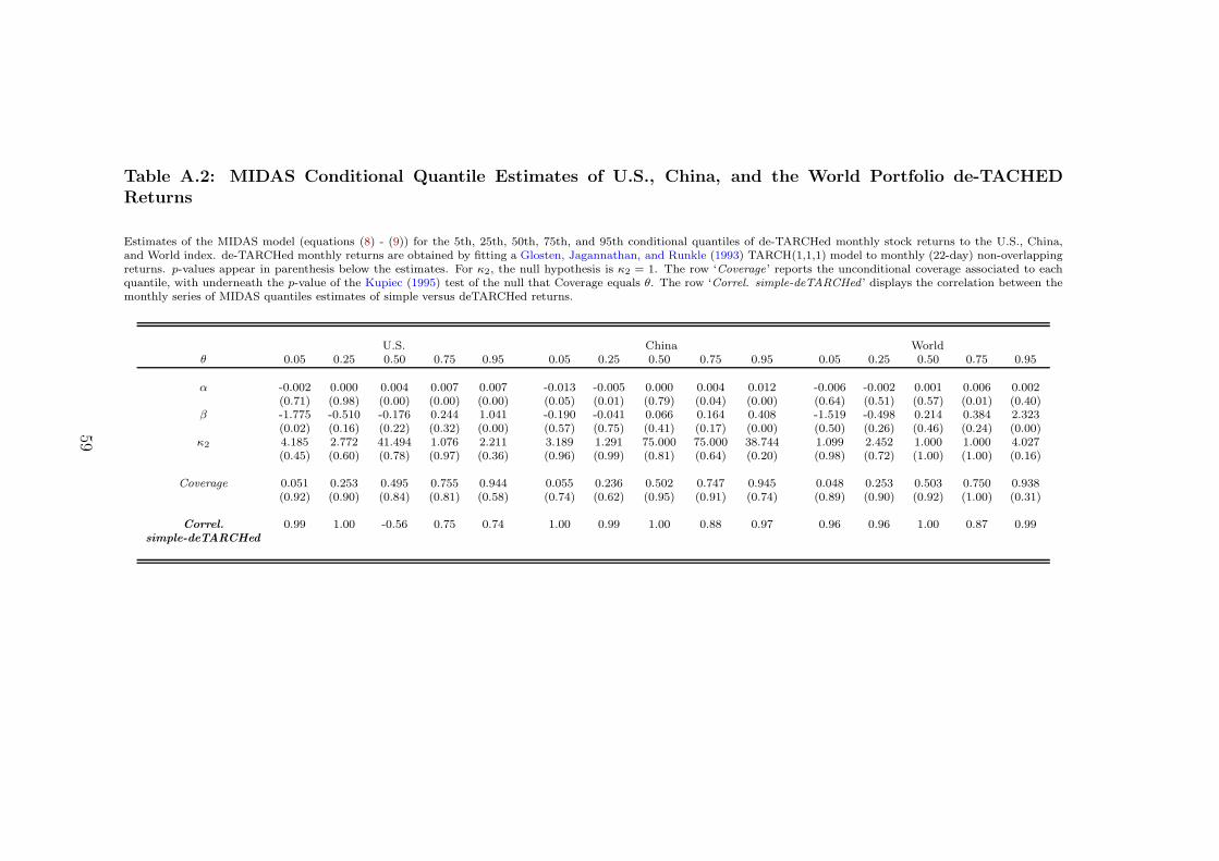
Table A.2: MIDAS Conditional Quantile Estimates of U.S., China, and the World Portfolio de-TACHEDReturns

Estimates of the MIDAS model (equations (8) - (9)) for the 5th, 25th, 50th, 75th, and 95th conditional quantiles of de-TARCHed monthly stock returns to the U.S., China,and World index. de-TARCHed monthly returns are obtained by fitting a Glosten, Jagannathan, and Runkle (1993) TARCH(1,1,1) model to monthly (22-day) non-overlappingreturns. p-values appear in parenthesis below the estimates. For κ2, the null hypothesis is κ2 = 1. The row ‘Coverage’ reports the unconditional coverage associated to eachquantile, with underneath the p-value of the Kupiec (1995) test of the null that Coverage equals θ. The row ‘Correl. simple-deTARCHed ’ displays the correlation between themonthly series of MIDAS quantiles estimates of simple versus deTARCHed returns.

U.S. China Worldθ 0.05 0.25 0.50 0.75 0.95 0.05 0.25 0.50 0.75 0.95 0.05 0.25 0.50 0.75 0.95

α -0.002 0.000 0.004 0.007 0.007 -0.013 -0.005 0.000 0.004 0.012 -0.006 -0.002 0.001 0.006 0.002(0.71) (0.98) (0.00) (0.00) (0.00) (0.05) (0.01) (0.79) (0.04) (0.00) (0.64) (0.51) (0.57) (0.01) (0.40)

β -1.775 -0.510 -0.176 0.244 1.041 -0.190 -0.041 0.066 0.164 0.408 -1.519 -0.498 0.214 0.384 2.323(0.02) (0.16) (0.22) (0.32) (0.00) (0.57) (0.75) (0.41) (0.17) (0.00) (0.50) (0.26) (0.46) (0.24) (0.00)

κ2 4.185 2.772 41.494 1.076 2.211 3.189 1.291 75.000 75.000 38.744 1.099 2.452 1.000 1.000 4.027(0.45) (0.60) (0.78) (0.97) (0.36) (0.96) (0.99) (0.81) (0.64) (0.20) (0.98) (0.72) (1.00) (1.00) (0.16)

Coverage 0.051 0.253 0.495 0.755 0.944 0.055 0.236 0.502 0.747 0.945 0.048 0.253 0.503 0.750 0.938(0.92) (0.90) (0.84) (0.81) (0.58) (0.74) (0.62) (0.95) (0.91) (0.74) (0.89) (0.90) (0.92) (1.00) (0.31)

Correl. 0.99 1.00 -0.56 0.75 0.74 1.00 0.99 1.00 0.88 0.97 0.96 0.96 1.00 0.87 0.99simple-deTARCHed

59

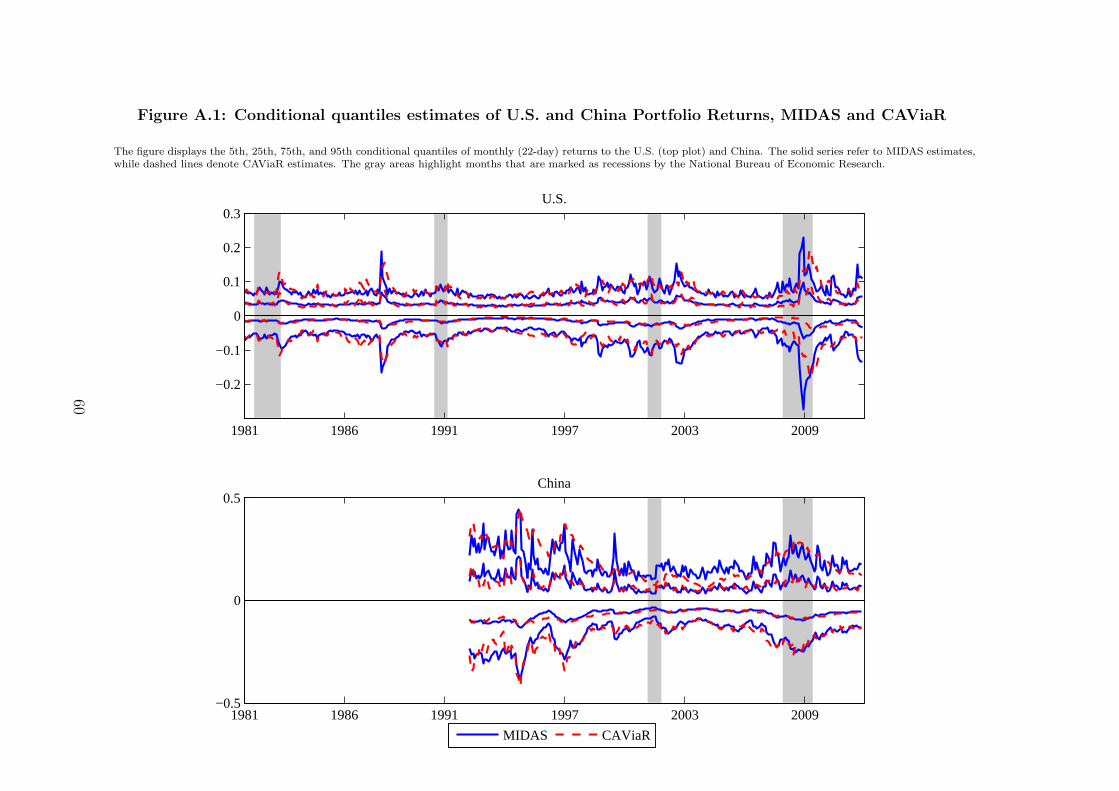
Figure A.1: Conditional quantiles estimates of U.S. and China Portfolio Returns, MIDAS and CAViaR

The figure displays the 5th, 25th, 75th, and 95th conditional quantiles of monthly (22-day) returns to the U.S. (top plot) and China. The solid series refer to MIDAS estimates,while dashed lines denote CAViaR estimates. The gray areas highlight months that are marked as recessions by the National Bureau of Economic Research.

U.S.

1981 1986 1991 1997 2003 2009

−0.2

−0.1

0

0.1

0.2

0.3

China

1981 1986 1991 1997 2003 2009−0.5

0

0.5

MIDAS CAViaR

60

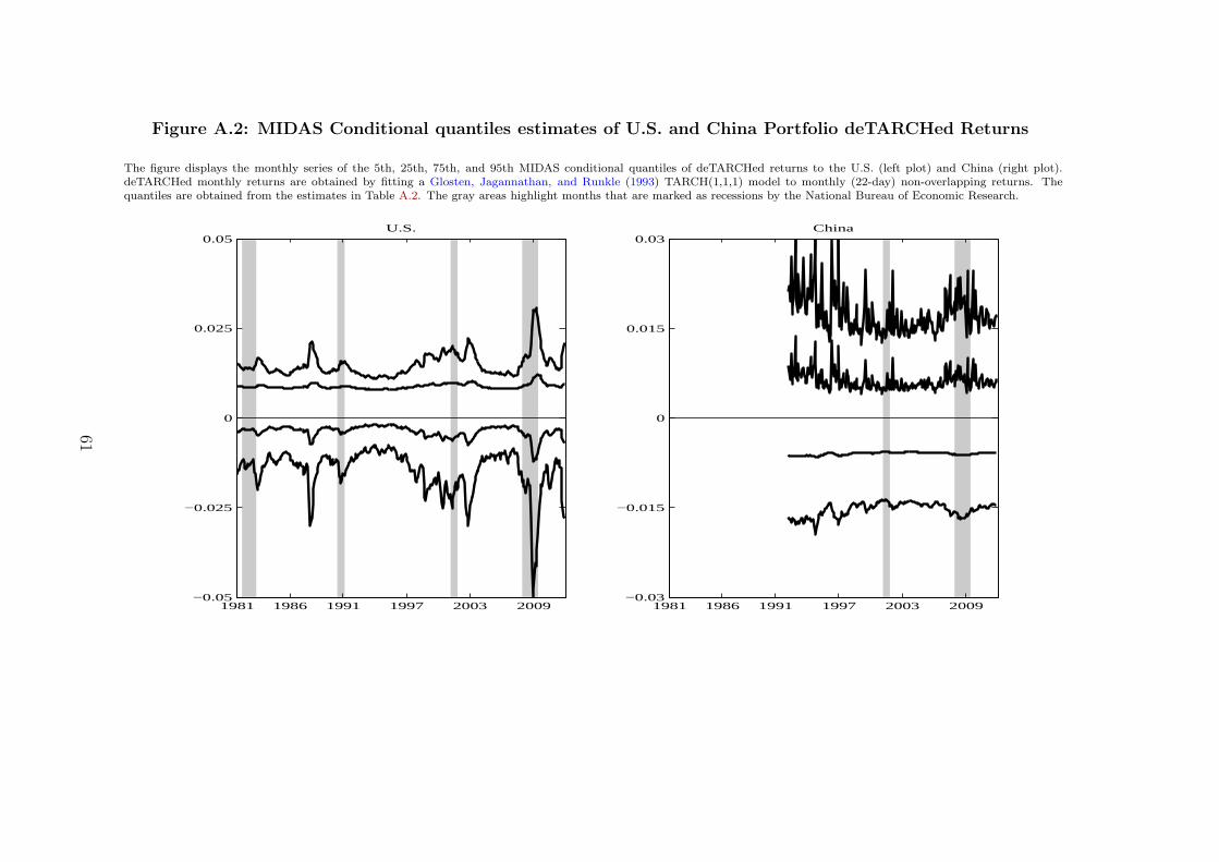
Figure A.2: MIDAS Conditional quantiles estimates of U.S. and China Portfolio deTARCHed Returns

The figure displays the monthly series of the 5th, 25th, 75th, and 95th MIDAS conditional quantiles of deTARCHed returns to the U.S. (left plot) and China (right plot).deTARCHed monthly returns are obtained by fitting a Glosten, Jagannathan, and Runkle (1993) TARCH(1,1,1) model to monthly (22-day) non-overlapping returns. Thequantiles are obtained from the estimates in Table A.2. The gray areas highlight months that are marked as recessions by the National Bureau of Economic Research.

U.S.

1981 1986 1991 1997 2003 2009−0.05

−0.025

0

0.025

0.05China

1981 1986 1991 1997 2003 2009−0.03

−0.015

0

0.015

0.03

61