Embed Size (px)
Citation preview

1
Auxiliary Materials for Paper
Widespread Decline in Greenness of Amazonian Vegetation Due
to the 2010 Drought
Liang Xu,1*
Arindam Samanta,2*
Marcos H. Costa,3
Sangram Ganguly,4 Ramakrishna R.
Nemani,5 and Ranga B. Myneni
1
1 Department of Geography and Environment, Boston University, Boston, MA 02215,
USA
2 Atmospheric and Environmental Research Inc., Lexington, MA 02421
2 Federal University of Viçosa (UFV), Av. P. H. Rolfs, s/n, Viçosa, MG, CEP 36570-000,
Brazil
3 Bay Area Environmental Research Institute, NASA Ames Research Center, Mail Stop
242-2, Moffett Field, CA, 94035, USA
4 Biospheric Science Branch, NASA Ames Research Center, Moffett Field, CA 94035,
USA
*These authors contributed equally to this work
Author for correspondence
Arindam Samanta
Atmospheric and Environmental Research Inc.
131 Hartwell Avenue, Lexington, MA 02421
Telephone: 617-852-5256
Fax: 781-761-2299
Email: [email protected]
Revised for Geophysical Research Letters
03-02-2011
2
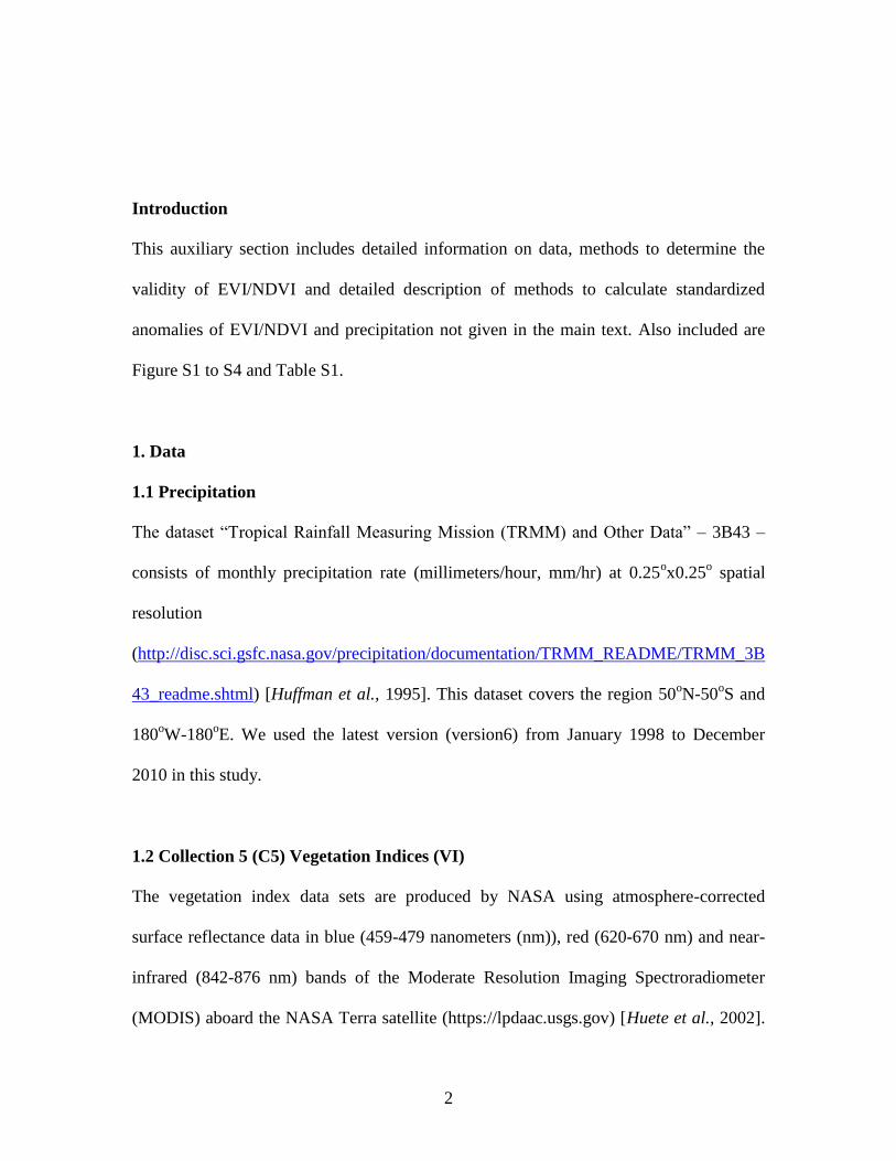
Introduction
This auxiliary section includes detailed information on data, methods to determine the
validity of EVI/NDVI and detailed description of methods to calculate standardized
anomalies of EVI/NDVI and precipitation not given in the main text. Also included are
Figure S1 to S4 and Table S1.
1. Data
1.1 Precipitation
The dataset “Tropical Rainfall Measuring Mission (TRMM) and Other Data” – 3B43 –
consists of monthly precipitation rate (millimeters/hour, mm/hr) at 0.25ox0.25
o spatial
resolution
(http://disc.sci.gsfc.nasa.gov/precipitation/documentation/TRMM_README/TRMM_3B
43_readme.shtml) [Huffman et al., 1995]. This dataset covers the region 50oN-50
oS and
180oW-180
oE. We used the latest version (version6) from January 1998 to December
2010 in this study.
1.2 Collection 5 (C5) Vegetation Indices (VI)
The vegetation index data sets are produced by NASA using atmosphere-corrected
surface reflectance data in blue (459-479 nanometers (nm)), red (620-670 nm) and near-
infrared (842-876 nm) bands of the Moderate Resolution Imaging Spectroradiometer
(MODIS) aboard the NASA Terra satellite (https://lpdaac.usgs.gov) [Huete et al., 2002].

3
The MODIS vegetation index product suite consists of Normalized Difference Vegetation
Index (NDVI) and Enhanced Vegetation Index (EVI). NDVI is a radiometric measure of
photosynthetically active radiation (400-700 nm) absorbed by canopy chlorophyll, and
therefore, is a good surrogate measure of the physiologically functioning surface
greenness level in a region [Myneni et al., 1995]. NDVI has been used in many studies of
vegetation dynamics in the Amazon [Asner et al., 2000; Dessay et al., 2004]. EVI
generally correlates well with ground measurements of photosynthesis and found to be
especially useful in high biomass tropical broadleaf forests like the Amazon [Huete et al.,
2002; 2006]. The latest versions of NDVI and EVI from the Terra MODIS instrument,
called Collection 5 (C5), are used in this study.
The dataset “Vegetation Indices 16-Day L3 Global 1km” – MOD13A2 contains EVI and
NDVI at 1x1km2 spatial resolution and 16-day frequency. This 16-day frequency arises
from compositing, i.e. assigning one best-quality EVI and NDVI value to represent a 16-
day period. This dataset is available in tiles (10ox10
o at the equator) of Sinusoidal
projection – 16 such tiles cover the Amazon region (approximately 10oN-20
oS and 80
oW-
45oW). These were obtained from the NASA Land Processes Data Active Archive Center
(LP DAAC) (https://lpdaac.usgs.gov) for the period February 2000 to December 2010.
1.2.1 VI data quality
The quality of 16-day vegetation index data (EVI and NDVI) in each 1x1km2 pixel can
be assessed using the accompanying 16-bit quality flags. Sets of bits, from these 16 bits,
4
are assigned to flags pertaining to clouds and aerosols, as well as, flags that provide
aggregate measures of data quality called VI Usefulness Indices. Cloud quality flags are
single bit (binary) flags indicating the presence (1) or absence (0) of clouds. There are
two binary cloud quality flags – “Adjacent cloud detected” (bit 8), “Mixed Clouds” (bit
10), and “Possible Shadows” (bit 15). The aerosol quality flag, 2 bits in precision,
provides information on aerosol content, and is named “Aerosol quantity”. It occupies bit
positions 6 through 7. The aerosol quality flag can have one of four values –
“Climatology” (00), “Low” (01), “Average” (10) and “High” (11). “Low”, “Average”
and “High” refer to aerosol optical thickness (AOT) at 550 nm less than 0.2, between 0.2
and 0.5, and greater than 0.5, respectively [Vermote and Vermuelen, 1999]. On the other
hand, “Climatology” indicates that the actual AOT is unknown, most likely due to
presence of clouds, and climatological (long-term average) AOT is used in the process of
atmospheric correction. The VI Usefulness flag, 4 bits in precision, provides an aggregate
measure of VI quality. It occupies bit positions – bits 2 through 5 – and can have values
from 0 (0000 – best quality) to 15 (1111 – not useful).
Determination of VI validity: The presence of clouds (adjacent clouds and mixed clouds)
“obscures” the surface in a radiometric sense, thus corrupting inferred VI values. In
addition, two types of aerosol loadings typically corrupt data – climatology and high
aerosols. Use of aerosol climatology indicates that the actual aerosol content is unknown,
most likely due to the presence of clouds, and aerosol correction was performed using
historical or climatological aerosol optical thickness (AOT) data [Vermote and
Vermuelen, 1999]. Moreover, atmospheric correction methods are ineffective for high

5
aerosol loadings (AOT > 0.5), especially in the shorter red and blue spectral [Vermote
and Kotchenova, 2008].
Based on the above information, each 1x1km2 16-day pixel is considered valid when (a)
VI data is produced – “MODLAND_QA” equals 0 (good quality) or 1 (check other QA),
(b) VI Usefulness is between 0 and 11, (c) Clouds are absent – “Adjacent cloud detected”
(0), “Mixed Clouds” (0), “Possible Shadows” (0), and (d) Aerosol content is low or
average – “Aerosol Quantity” (1 or 2). Note that “MODLAND_QA” checks whether VI
is produced or not, and if produced, its quality is good or whether other quality flags
should also be checked. Besides, VI Usefulness Indices 0 to 11 essentially include all VI
data. Thus, these two conditions serve as additional checks.
1.3 Land cover
Land cover information was obtained from the “MODIS Terra Land Cover Type Yearly
L3 Global 1 km SIN Grid” product – MOD12Q1. This is the official NASA C5 land
cover data set (https://lpdaac.usgs.gov/) [Friedl et al., 2010]. It consists of five land cover
classification schemes at 1x1km2 spatial resolution. The International Geosphere
Biosphere Programme (IGBP) land cover classification scheme was used to identify
forest and non-forest vegetated pixels in the Amazon region (see Fig. S2).
2. Methods
2.1 Standardized Anomaly
Standardized anomalies (anomaly divided by the standard deviation) of precipitation, and
VI (NDVI and EVI) are calculated for 2005 and 2010 pixel-by-pixel as, a = (x-m)/s,

6
where a is the 2005 (or, 2010) standardized anomaly of a given quantity (precipitation,
NDVI, EVI) calculated from its value in 2005 (or, 2010) x and long term mean m and
standard deviation s over a reference period. The reference period is 2000-2009, but
excluding 2005. Thus, 2005 and 2010 are not part of the reference period.
2.1.1 VI Standardized Anomaly
For each year, we use six 16-day VI (NDVI or EVI) composites – 177 through 257 –
covering the July-September (JAS) period. The VI value of a pixel is considered valid if
it is free of atmospheric contamination due to clouds (adjacent clouds, mixed clouds and
cloud shadows) and aerosols (climatology and high aerosols), which is determined by
examining the corresponding quality flags (cf. Section 1.2.1). For each year, the JAS
mean VI is calculated using only valid values. The mean (m) and standard deviation (s)
are evaluated over the base period, years 2000 to 2009, but excluding 2005. Finally, if the
2005(or, 2010) JAS mean VI (x) exists, the 2005 (or, 2010) standardized anomaly is
calculated.
We found blocks and strips of anomalously low VI values (especially in NDVI data) even
after screening for clouds and aerosol contamination using quality flags, as described
above. This points to further residual atmospheric corruption effects. To remove these
artifacts, we estimated the 11-year (2000 to 2010) mean NDVI for each 16-day composite
and screened VI values that were two standard deviations (95% envelope) or more below
the mean. This additional filtering greatly reduced blocks and strips of anomalously low
VI values.

7
2.1.2 Precipitation Standardized Anomaly
The monthly precipitation value is considered “valid” if it is not equal to -9999. If all
three monthly – July, August and September - precipitation values are valid, the total of
the three represents the quarterly (JAS) cumulative value. Else, the pixel is tagged and
not used in further calculations. The long term mean (m) and standard deviation (s) of
JAS cumulative precipitation are evaluated over the period 1998-2009, but excluding
2005. Finally, if the 2005 (or, 2010) JAS cumulative precipitation (x) exists, the 2005 (or,
2010) standardized anomaly (a) is estimated. Pixels with precipitation anomalies less
than -1 standard deviation (std. dev.) are classified as drought-stricken.

8
References
Asner, G. P., A R. Townsend, and B. H. Braswell (2000), Satellite observation of El Nino
effects on Amazon forest phenology and productivity, Geophysical Research Letters,
27, 981-984.
Dessay, N. et al (2004), Comparative study of the 1982-1983 and 1997-1998 El Nino
events over different types of vegetation in South America, International Journal of
Remote Sensing, 25, 4063-4077, doi:10.1080/0143116031000101594.
Friedl, M. A., D. Sulla-Menashe, B. Tan, A. Schneider, N. Ramankutty, A. Sibley, and X.
Huang (2010), MODIS Collection 5 global land cover: Algorithm refinements and
characterization of new datasets. Rem. Sens. Environ., 114(1), 168-182.
Huete, A. R., K. Didan, T. Miura, E. Rodriguez, X. Gao, and L. Ferreira (2002),
Overview of the radiometric and biophysical performance of the MODIS vegetation
indices, Remote Sens. Environ., 83, 195-213.
Huete, A. R., K. Didan, Y. E. Shimabukuro, P. Ratana, S. R. Saleska, L. R. Hutyra, W. Z.
Yang, R. R. Nemani, and R. B. Myneni (2006), Amazon rainforests green-up with
sunlight in dry season, Geophys. Res. Lett., 33, L06405,
doi:10.1029/2005GL025583.
Huffman, G., R. Adler, B. Rudolf, U. Schneider, and P. Keehn (1995), Global
precipitation estimates based on a technique for combining satellite-based

9
estimates, rain-gauge analysis, and NWP model precipitation information, Journal
of Climate, 8(5), 1284-1295.
Myneni, R. B., F. G. Hall, P. J. Sellers, and A. L. Marshak (1995), The interpretation of
spectral vegetation indexes, IEEE Transactions on Geoscience and Remote Sensing,
33(2), 481-486.
Vermote, E. F., and S. Kotchenova (2008), Atmospheric correction for the mornitoring of
land surfaces, J. Geophys. Res., 113, D23S90, doi:10.1029/2007JD009662.
Vermote, E. F., and A. Vermuelen (1999), Atmospheric Correction Algorithm: Spectral
Reflectances (MOD09), MODIS Algorithm Theoretical Basis Document,
http://modis.gsfc.nasa.gov/data/atbd/atbd_mod08.pdf.

10
Figure Captions
Figure S1. Spatial patterns of July to September (JAS) 2010 and 2005 standardized
anomalies of precipitation.
Figure S2. Aggregated International Geosphere Biosphere Program landcover classes of
Amazonia at 0.05ox0.05
o spatial resolution, derived from the MODIS Collection 5 (C5)
landcover product.
Figure S3. Spatial patterns of drought impact on Amazonian vegetation in 2005 and
2010. (a) Vegetated areas where the July to September (JAS) precipitation anomalies are
less than -1 standard deviations (std.)) in 2010 that show greenness declines (JAS NDVI
anomalies less than -1 std.) and. (b) same as (a) but for EVI. (c) and (d) same as (a) and
(b), respectively, but for 2005.
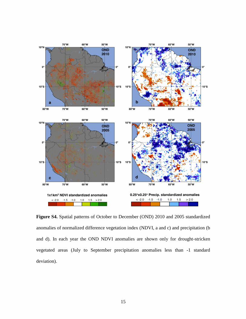
Figure S4. Spatial patterns of October to December (OND) 2010 and 2005 standardized
anomalies of normalized difference vegetation index (NDVI, a and c) and precipitation (b
and d). In each year the OND NDVI anomalies are shown only for drought-stricken
vegetated areas (July to September precipitation anomalies less than -1 standard
deviation).

11
Table Captions
Table S1. The 10 lowest stages recorded on the Rio Negro at the Manaus harbor, 1902-
2010 (n=109). Source: CPRM/ANA (Serviço Geológico do Brasil/Agência Nacional das
Águas - Brazil Geological Service/National Agency for Water). Return periods of
droughts were calculated by ranking, from low to high, the lowest level reached by the
river in each year of the time series of length n=109 (1902-2010), and calculating the
probability of occurrence by dividing the rank by n+1 (110). The return period is the
inverse of the probability of occurrence.

12
Figure S1. Spatial patterns of July to September (JAS) 2010 and 2005 standardized
anomalies of precipitation.

13
Figure S2. Aggregated International Geosphere Biosphere Program landcover classes of
Amazonia at 0.05ox0.05
o spatial resolution, derived from the MODIS Collection 5 (C5)
landcover product.

14
Figure S3. Spatial patterns of drought impact on Amazonian vegetation in 2005 and
2010. (a) Vegetated areas where the July to September (JAS) precipitation anomalies are
less than -1 standard deviations (std.)) in 2010 that show greenness declines (JAS NDVI
anomalies less than -1 std.) and. (b) same as (a) but for EVI. (c) and (d) same as (a) and
(b), respectively, but for 2005.
15
Figure S4. Spatial patterns of October to December (OND) 2010 and 2005 standardized
anomalies of normalized difference vegetation index (NDVI, a and c) and precipitation (b
and d). In each year the OND NDVI anomalies are shown only for drought-stricken
vegetated areas (July to September precipitation anomalies less than -1 standard
deviation).

16
Table S1. The 10 lowest stages recorded on the Rio Negro at the Manaus harbor, 1902-
2010 (n=109). Source: CPRM/ANA (Serviço Geológico do Brasil/Agência Nacional das
Águas - Brazil Geological Service/National Agency for Water). Return periods of
droughts were calculated by ranking, from low to high, the lowest level reached by the
river in each year of the time series of length n=109 (1902-2010), and calculating the
probability of occurrence by dividing the rank by n+1 (110). The return period is the
inverse of the probability of occurrence.