WILLIAM DUNHAM

THE CALCULUS

GALLERY

Masterpieces from Newton to Lebesgue

PRINCETON UNIVERSITY PRESS

PRINCETON AND OXFORD

Copynght © 2005 by Pnnceton University PressPublished by Pnnceton University Press, 41 William Street,

Princeton, New Jersey 08540In the United Kingdom Pnnceton University Press, 3 Market Place,

Woodstock, Oxfordshire OX20 ISY

All Rights Reserved

Library of Congress Cataloging-in-Publication DataDunham, William, 1947-

The calculus gallery masterpieces from Newton toLebesgue / William Dunham

p cmIncludes bibliographical references and mdex

ISBN 0-691-09565-5 (acid-free paper)

Calculus-History I TitleQA303 2 D86 2005

515---dc222004040125

British Library Catalogmg-in-Publication Data is available

This book has been composed in Berkeley Book

Printed on acid-free paper 00

pup pnnceton edu

Pnnted in the United States of America

3 5 7 9 10 8 6 4 2

In memory of Norman Levine

tr

Contents

Illustrations ix

Acknowledgments xiii

INTRODUCTION

CHAPTER INewton 5

CHAPTER 2Leibniz 20

CHAPTER 3The Bernoullis 35

CHAPTER 4Euler 52

CHAPTER 5First Interlude 69

CHAPTER 6Cauchy 76

CHAPTER 7Riemann 96

CHAPTER 8Liouville 116

CHAPTER 9Weierstrass 128

CHAPTER 10Second Interlude 149

VII

viii CONTENTS

CHAPTER IICantor 158

CHAPTER 12Volterra 170

CHAPTER 13Baire 183

CHAPTER 14Lebesgue 200

Afterword 220

Notes 223

Index 233

Illustrations

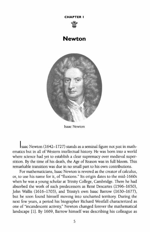
Portrait of Isaac Newton 5

Figure 1.1 12

Figure 1.2 13

Figure 1.3 16

Newton's series for sine andcosine (1669) 18

Portrait of GottfriedWilhelm Leibniz 20

Leibniz's first paper on differentialcalculus (1684) 22

Figure 2.1 23

Figure 2.2 24

Figure 2.3 25

Figure 2.4 26

Figure 2.5 27

Figure 2.6 28

Figure 2.7 30

Figure 2.8 31

Figure 2.9 32

Portraits of Jakob and JohannBernoulli 35

Figure 3.1 42

Figure 3.2 47

Johann Bernoulli's integraltable (1697) 48

Portrait of Leonhard Euler 52

Portrait ofAugustin-Louis Cauchy 76

Figure 6.1 81

IX

X ILLUSTRATIONS

Cauchy's proof of the fundamentaltheorem of calculus (1823) 89

Portrait of Georg FriedrichBernhard Riemann 96

Figure 7.1 97

Figure 7.2 99

Figure 7.3 102

Figure 7.4 103

Figure 7.5 104

Figure 7.6 108

Figure 7.7 109

Figure 7.8 110

Portrait of Joseph Liouville I 16

Figure 8.1 I 18

Portrait of Karl Weierstrass 128

Figure 9.1 131

Figure 9.2 133

Figure 9.3 134

Figure 9.4 135

Figure 9.5 136

Figure 9.6 138

Weierstrass's pathologicalfunction (1872) 142

Figure 9.7 143

Figure 9.8 147

Figure 10.1 150

Figure 10.2 153

Figure 10.3 154

Portrait of Georg Cantor 158

Figure I 1.1 162

Figure I 1.2 163

ILLUSTRATIONS XI

Portrait ofVito Volterra 170

Figure 12.1 178

Figure 12.2 179

Portrait of Rene Baire 183

Figure 13.1 185

Figure 13.2 185

The Baire category theorem (1899) 190

Portrait of Henri Lebesgue 200

Figure 14.1 203

Figure 14.2 211

Figure 14.3 213

Lebesgue's proof of the boundedconvergence theorem (1904) 217

Acknowledgments

~iS book is the product of my year as the Class of 1932 ResearchProfessor at Muhlenberg College. I am grateful to Muhlenberg for thisopportunity, as I am to those who supported me in my application: TomBanchoff of Brown University, Don Bonar of Denison, Aparna Higgins ofthe University of Dayton, and Fred Rickey of West Point.

Once underway, my efforts received valuable assistance from computerwizard Bill Stevenson and from friends and colleagues in Muhlenberg'sDepartment of Mathematical Sciences: George Benjamin, Dave Nelson, ElynRykken, Linda McGuire, Greg Cicconetti, Margaret Dodson, Clif Kussmaul,Linda Luckenbill, and the recently retired John Meyer, who believed inthis project from the beginning.

This work was completed using the resources of Muhlenbergs TrexlerLibrary, where the efforts of Tom Gaughan, Martha Stevenson, and KarenGruber were so very helpful. I should mention as well my use of the excel­lent collections of the Fairchild-Martindale Library at Lehigh Universityand of the Fine Hall Library at Princeton.

Family members are a source of special encouragement in a job of thismagnitude, and I send love and thanks to Brendan and Shannon, to mymother, to Ruth and Bob Evans, and to Carol Dunham in this regard.

I would be remiss not to acknowledge George Poe, Professor ofFrench at the University of the South, whose detective work in trackingdown obscure pictures would make Auguste Dupin envious. I am likewiseindebted to Russell Howell of Westmont College, who proved once againthat he could have been a great mathematics editor had he not become agreat mathematics professor.

A number of individuals deserve recognition for turning my manu­script into a book. Among these are Alison Kalett, Dimitri Karetnikov,Carmina Alvarez, Beth Gallagher, Gail Schmitt, and most of all VickieKearn, senior mathematics editor at Princeton University Press, who over­saw this process with her special combination of expertise and friendship.

Lastly, I thank my wife and colleague Penny Dunham. She created thebook's diagrams and proVIded helpful suggestions as to its contents. Herpresence has made this understanding, and the past 35 years, so much fun.

W DunhamAllentown, PA

xiii

THE CALCULUS

GALLERY

~ff~

INTRODUCTION

"TIhe calculus," wrote John von Neumann (1903-1957), "was the

first achievement of modern mathematics, and it is difficult to overesti­mate its importance" [1].

Today, more than three centuries after its appearance, calculus contin­ues to warrant such praise. It is the bridge that carries students from thebasics of elementary mathematics to the challenges of higher mathematicsand, as such, provides a dazzling transition from the finite to the infinite,from the discrete to the continuous, from the superficial to the profound.So esteemed is calculus that its name is often preceded by "the," as in vonNeumann's observation above. This gives "the calculus" a status akin to"the law"-that is, a subject vast, self-contained, and awesome.

Like any great intellectual pursuit, the calculus has a rich history anda nch prehistory. Archimedes of Syracuse (ca. 287-212 BCE) found certainareas, volumes, and surfaces with a technique we now recognize as proto­integration. Much later, Pierre de Fermat (1601-1665) determined slopesof tangents and areas under curves in a remarkably modern fashion. Theseand many other illustrious predecessors brought calculus to the thresholdof existence.

Nevertheless, this book is not about forerunners. It goes without say­ing that calculus owes much to those who came before, just as modern artowes much to the artists of the past. But a specialized museum-theMuseum of Modern Art, for instance-need not devote room after roomto premodern influences. Such an institution can, so to speak, start in themiddle. And so, I think, can I.

Thus I shall begin with the two seventeenth-century scholars, IsaacNewton 0642-1727) and Gottfried Wilhelm Leibniz (1646-1716), whogave birth to the calculus. The latter was first to publish his work in a 1684paper whose title contained the Latin word calculi (a system of calculation)that would attach itself to this new branch of mathematics. The first text­book appeared a dozen years later, and the calculus was here to stay.

As the decades passed, others took up the challenge. Prominentamong these pioneers were the Bernoulli brothers, Jakob 0654-1705)and Johann 0667-1748), and the incomparable Leonhard Euler 0707­1783), whose research filled many thousands of pages with mathematics

2 INTRODUCTION

of the highest quality. Topics under consideration expanded to includelimits, derivatives, integrals, infinite sequences, infinite series, and more.This extended body of material has come to be known under the generalrubric of "analysis."

With increased sophistication came troubling questions about theunderlYIng logic. Despite the power and utility of calculus, it rested upona less-than-certain foundation, and mathematicians recognized the needto recast the subject in a precise, rigorous fashion after the model of Euclidsgeometry. Such needs were addressed by nineteenth-century analystslike Augustin-Louis Cauchy (1789-1857), Georg Friedrich BernhardRiemann (1826-1866), Joseph Liouville (1809-1882), and Karl Weier­strass (1815-1897). These individuals worked with unprecedented care,taking pains to define their terms exactly and to prove results that hadhitherto been accepted uncritically.

But, as often happens in science, the resolution of one problemopened the door to others. Over the last half of the nineteenth century,mathematicians employed these logically rigorous tools in concocting ahost of strange counterexamples, the understanding of which pushedanalysis ever further toward generality and abstraction. This trend wasevident in the set theory of Georg Cantor (1845-1918) and in the subse­quent achievements of scholars like Vito Volterra (1860-1940), Rene Baire(1874-1932), and Henri Lebesgue (1875-1941).

By the early twentieth century, analysis had grown into an enormouscollection of ideas, definitions, theorems, and examples-and had devel­oped a characteristic manner of thinking-that established it as a mathe­matical enterprise of the highest rank.

What follows is a sampler from that collection. My goal is to examinethe handiwork of those individuals mentioned above and to do so in amanner faithful to the originals yet comprehensible to a modern reader. Ishall discuss theorems illustrating the development of calculus over itsformative years and the genius of its most illustrious practitioners. Thebook will be, in short, a "great theorems" approach to this fascinatingstory.

To this end I have restricted myself to the work of a few representativemathematicians. At the outset I make a full disclosure: my cast of characterswas dictated by personal taste. Some whom I have included, like Newton,Cauchy, Weierstrass, would appear in any book with similar objectives.Some, like Liouville, Volterra and Baire, are more idiosyncratic. And others,like Gauss, Bolzano, and Abel, failed to make my cut.

INTRODUCTION 3

Likewise, some of the theorems I discuss are known to any mathemat­ically literate reader, although their original proofs may come as a surpriseto those not conversant with the history of mathematics. Into this categoryfall Leibniz's barely recognizable derivation of the "Leibniz series" from1673 and Cantor's first but less-well-known proof of the nondenumer­ability of the continuum from 1874. Other theorems, although part of thefolklore of mathematics, seldom appear in modern textbooks; here I amthinking of a result like Weierstrass!> everywhere continuous, nowhere dif­ferentiable function that so astounded the mathematical world when itwas presented to the Berlin Academy in 1872. And some of my choices,

p sin(lnx)I concede, are downright quirky. Euler's evaluation of Jo dx, for

lnxexample, is included simply as a demonstration of his analytic wizardry.

Each result, from Newton's derivation of the sine series to the appear­ance of the gamma function to the Baire category theorem, stood at theresearch frontier of its day. Collectively, they document the evolution ofanalysis over time, with the attendant changes in style and substance. Thisevolution is striking, for the difference between a theorem from Lebesguein 1904 and one from Leibniz in 1690 can be likened to the differencebetween modern literature and Beowulf. Nonetheless-and this is critical­I believe that each theorem reveals an ingenuity worthy of our attentionand, even more, of our admiration.

Of course, trying to characterize analysis by examining a few theoremsis like trying to characterize a thunderstorm by collecting a few raindrops.The impression conveyed will be hopelessly incomplete. To undertakesuch a project, an author must adopt some fairly restnctive guidelines.

One of mine was to resist writing a comprehensive history of analysis.That is far too broad a mission, and, in any case, there are many works thatdescribe the development of calculus. Some of my favorites are mentionedexpliCitly in the text or appear as sources in the notes at the end of the book.

A second decision was to exclude topics from both multivariate calcu­lus and complex analysis. This may be a regrettable choice, but I believe itis a defensible one. It has imposed some manageable boundaries upon thecontents of the book and thereby has added coherence to the tale. Simul­taneously, this restriction should minimize demands upon the reader'sbackground, for a volume limited to topics from univariate, real analysisshould be understandable to the widest possible audience.

This raises the issue of prerequisites. The book's objectives dictate thatI include much technical detail, so the mathematics necessary to follow

4 INTRODUCTION

these theorems is substantial. Some of the early results require consider­able algebraic stamina in chasing formulas across the page. Some of thelater ones demand a refined sense of abstraction. All in all, I would notrecommend this for the mathematically faint-hearted.

At the same time, in an attempt to favor clarity over conciseness, Ihave adopted a more conversational style than one would find in a stan­dard text. I intend that the book be accessible to those who have majoredor minored in college mathematics and who are not put off by an integralhere or an epSilon there. My goal is to keep the prerequisites as modest asthe topics permit, but no less so. To do otherwise, to water down the con­tent, would defeat my broader purpose.

So, this is not primarily a biography of mathematicians, nor a historyof calculus, nor a textbook. I say this despite the fact that at times I pro­vide biographical information, at times I discuss the history that ties onetopiC to another, and at times I introduce unfamiliar (or perhaps long for­gotten) ideas in a manner reminiscent of a textbook. But my foremostmotivation is Simple: to share some favorite results from the rich history ofanalysis.

And this brings me to a final observation.In most disciplines there is a tradition of studying the major works of

illustnous predecessors, the so-called "masters" of the field. Students of lit­erature read Shakespeare; students of music listen to Bach. In mathematicssuch a tradition is, if not entirely absent, at least fairly uncommon. Thisbook is meant to address that situation. Although it is not intended as a his­tory of the calculus, I have come to regard it as a gallery of the calculus.

To this end, I have assembled a number of masterpieces, although theseare not the paintings of Rembrandt or Van Gogh but the theorems of Euleror Riemann. Such a gallery may be a bit unusual, but its objective is that ofall worthy museums: to serve as a repository of excellence.

Like any gallery, this one has gaps in its collection. Like any gallery,there is not space enough to display all that one might wish. These limi­tations notwithstanding, a visitor should come away enriched by anappreciation of genius. And, in the final analysis, those who stroll amongthe exhibits should experience the mathematical imagination at its mostprofound.

CHAPTER I

Newton

Isaac Newton

Isaac Newton (1642-1727) stands as a seminal figure not Just in math­ematics but in all of Western intellectual history. He was born into a worldwhere science had yet to establish a clear supremacy over medieval super*stition. By the time of his death, the Age of Reason was in full bloom. Thisremarkable transition was due in no small part to his own contributions.

For mathematicians, Isaac Newton is revered as the creator of calculus,or, to use his name for it, of "fluxions." Its origin dates to the mid-1660swhen he was a young scholar at Trinity College, Cambridge. There he hadabsorbed the work of such predecessors as Rene Descartes (1596--1650),John Wallis (1616-1703), and Trinitys own Isaac Barrow (1630-1677),but he soon found himself mOVIng into uncharted territory. During thenext few years, a period his biographer Richard Westfall characterized asone of "incandescent actiVIty,n Newton changed forever the mathematicallandscape [11. By 1669, Barrow himself was describing his colleague as

5

6 CHAPTER I

"a fellow of our College and very young ... but of an extraordinary geniusand proficiency" [2].

In this chapter, we look at a few of Newton's early achievements: hisgeneralized binomial expansion for turning certain expressions into infiniteseries, his technique for finding inverses of such series, and his quadraturerule for determining areas under curves. We conclude with a spectacularconsequence of these: the series expanSion for the sine of an angle. New­tons account of the binomial expansion appears in his epistola prior, a let­ter he sent to Leibniz in the summer of 1676 long after he had done theoriginal work. The other discussions come from Newtons 1669 treatise Deanalysi per aequationes numero terminorum infinitas, usually called simplythe De analysi.

Although this chapter is restricted to Newton's early work, we note that"early" Newton tends to surpass the mature work of just about anyone else.

GENERALIZED BINOMIAL EXPANSION

By 1665, Isaac Newton had found a simple way to expand-his wordwas "reduce"-binomial expressions into series. For him, such reductionswould be a means of recasting binomials in alternate form as well as anentryway into the method of fluxions. This theorem was the starting pointfor much of Newton's mathematical innovation.

As described in the epistola prior, the issue at hand was to reduce thebinomial (P + PQ)mln and to do so whether min "is integral or (so to speak)fractional, whether positive or negative" [3]. This in itself was a bold ideafor a time when exponents were suffiCiently unfamiliar that they had first

to be explained, as Newton did by stressing that "instead of.[O., va, ~,etc. I write a1l2 , a1l3 , a5/3 , and instead of 1/a, 1/aa, 1/a3 , I write a-I, a-2 ,

a-3" [4]. Apparently readers of the day needed a gentle reminder.Newton discovered a pattern for expanding not only elementary bino-

mials like (1 + X)5 but more sophisticated ones like ~ 1 5 = (1 + X)-5/3.3 (l + x)

The reduction, as Newton explained to Leibniz, obeyed the rule

(P + PQ)m/n = pm/n + m AQ + m - n BQn 2n

m - 2n m - 3n+ CQ+ DQ+etc., (1)3n 4n

NEWTON 7

where each of A, B, C, ... represents the previous tenn, as will be illus­trated below. This is his famous binomial expansion, although perhaps inan unfamiliar guise.

. ..J 2 2 [2 2 ( 2 2 )]112Newton proVIded the example of e + x = e + e x / e .

x2

Here, p= e2 , Q = -2 ' m =1, and n =2. Thus,e

2 2 2..J 2 2 2 112 1 x 1 x 1 xe +x = (e) +-A- --B---C-2 e2 4 e2 2 e2

5 x 2

--D-----8 e2

To identify A, B, C, and the rest, we recall that each is the immediatelypreceding tenn. Thus, A =(e2)112 =e, giving us

2

Likewise B is the previous tenn-Le., B =~ -so at this stage we have2e

x4 x 6

The analogous substitutions yield C = - -3 and then D =--5 . Working8e 16e

from left to right in this fashion, Newton arrived at

2 2 x2X

4 x 6 5x8

.Je +x =e+---+-----+ .. ·.2e 8e3 16e5 128e7

Obviously, the technique has a recursive flavor: one finds the coeffi­cient of x8 from the coefficient of x6 , which in turn requires the coefficientof x4 , and so on. Although the modern reader is probably accustomed to a"direct" statement of the binomial theorem, Newton's recursion has an un­deniable appeal, for it streamlines the arithmetic when calculating a nu­merical coefficient from its predecessor.

For the record, it is a simple matter to replace A, B, C, ... by theireqUivalent expressions in terms of P and Q, then factor the common

8 CHAPTER I

pm/n from both sides of (1), and so arrive at the result found in today'stexts:

Newton likened such reductions to the conversion of square rootsinto infinite decimals, and he was not shy in touting the benefits of theoperation. "It is a convenience attending infinite series," he wrote in1671,

that all kinds of complicated terms ... may be reduced to the classof simple quantities, i.e., to an infinite series of fractions whose nu­merators and denominators are simple terms, which will thus befreed from those difficulties that in their original form seem'd al­most insuperable. [5]

To be sure, freeing mathematics from insuperable difficulties is a worthyundertaking.

One additional example may be helpful. Consider the expansion of

1~ , which Newton put to good use in a result we shall discuss later

\11- x-in the chapter. We first write this as (l - x2)-l!2, identify m =- 1, n =2,and Q =- x2 , and apply (2):

1 = 1+(-~)(-X2)+ (-1/2)(-3/2) (_X2)2~ 2 2x1

(-1/2)(-3/2)(-5/2) ( 2)3+ -x

3x2x1

+ (-1/2)(-3/2)(-5/2)(-7/2) (_X 2)4+ ...

4x3x2x1

1 2 3 4 5 6 35 8= 1+ - x + - x + - x + - x +.... (3)2 8 16 128

NEWTON 9

Newton would "check" an expansion like (3) by squaring the seriesand examining the answer. If we do the same, restricting our attention toterms of degree no higher than x8 , we get

[1 2 3 4 5 6 35 8 ]

1+ 2" x +"8 x + 16 x + 128 x + ...

[1 2 3 4 5 6 35 8 ]

X 1+-x +-x +-x +--x + ...2 8 16 128

1 2 4 6 8= + X + X + X + X + ...,

where all of the coefficients miraculously tum out to be 1 (try it!). The re­sulting product, of course, is an infinite geometric series with common ratio

1x2 which, by the well-known formula, sums to --2 . But if the square of the

I-x1 1

series in (3) is --2 ' we conclude that that series itself must be ,,----------r'I-x ~1-x-

Voila!Newton regarded such calculations as compelling evidence for his gen­

eral result. He asserted that the "common analysis performed by means ofequations of a finite number of terms" may be extended to such infinite ex­pressions "albeit we mortals whose reasoning powers are confined withinnarrow limits, can neither express nor so conceive all the terms of theseequations, as to know exactly from thence the quantities we want" [6].

INVERTING SERIES

Having described a method for reducing certain binomials to infiniteseries of the form z =A + Bx + Cx2 + Dx3 + .. " Newton next sought away of finding the series for x in terms of z. In modem terminology, hewas seeking the inverse relationship. The resulting technique involves abit of heavy algebraic lifting, but it warrants our attention for it too willappear later on. As Newton did, we describe the inversion procedure bymeans of a specific example.

Beginning with the series z =x - x2 + x3 - x4 + .. " we rewrite it as

(x - x2 + x3 - x4 + ...) - z =0 (4)

and discard all powers of x greater than or equal to the quadratic. This, ofcourse, leaves x - Z = 0, and so the inverted series begins as x = z.

10 CHAPTER I

Newton was aware that discarding all those higher degree terms ren­dered the solution inexact. The exact answer would have the form x =Z + p,where p is a series yet to be determined. Substituting z + p for x in (4)gives

[(z + p) - (z + p)2 + (z + p)3 - (z + p)4 + ...J - z =0,

which we then expand and rearrange to get

[-Z2 + Z3 - Z4 + Z5 - ... j + [1 - 2z + 3z2 - 4z3+ 5z4 - Jp+ [-1 + 3z - 6z2 + lOz3 - ...Jp2 + [1 - 4z + lOz2 - jp3

+ [-1 + 5z - .. .]p4 + ... = O. (5)

Next, jettison the quadratic, cubic, and higher degree terms in p and solveto get

Z2_ Z3+ Z4_ Z5+ ...P= 2 3 .

1 - 2z + 3z - 4z + ...

Newton now did a second round of weeding, as he tossed out all butthe lowest power of Z in numerator and denominator. Hence p is approxi­

2

mately ~, so the inverted series at this stage looks like x = Z+ P= z + Z2.1

But P is not exactly Z2. Rather, we say p =Z2 + q, where q is a senes tobe determined. To do so, we substitute into (5) to get

[- Z2 + Z3 - Z4 + Z5 _ ...J + [1 - 2z + 3z2 - 4z3 + 5z4 - .. ·J(Z2 + q)

+ [-1 + 3z - 6z2 + lOz3 - ...J(Z2 + q)2 + [l - 4z + lOz2 - ... j

(Z2 + q)3 + [-1 + 5z - ... J(Z2 + q)4 + ... =O.

We expand and collect terms by powers of q:

[-Z3 + Z4 - Z6 + ... J + [1 - 2z + Z2 + 2z3 - ... jq

+[-1+3z-3z2-2z3+ ... j q2+.... (6)

As before, discard terms involving powers of q above the first, solve to

Z3 - Z4 + Z6 - ...get q = 2 3 ' and then drop all but the lowest degree

1- 2z + z + 2z + ...3

terms top and bottom to arrive at q =T· At this point, the series looks like

x = Z + Z2 + q = Z + Z2 + Z3.

NEWTON II

The process would be continued by substituting q =Z3 + r into (6).Newton, who had a remarkable tolerance for algebraic monotony, seemedable to continue such calculations ad infinitum (almost). But eventuallyeven he was ready to step back, examine the output, and seek a pattern.Newton put it this way: "Let it be observed here, by the bye, that when 5or 6 terms ... are known, they may be continued at pleasure for mostpart, by observing the analogy of the progression" [7].

For our example, such an examination suggests that x =Z + Z2 + Z3 +Z4 + Z5 + . . . is the inverse of the series Z =x - x2 + x3 - x4 + . . . withwhich we began.

In what sense can this be trusted? After all, Newton discarded most ofhis terms most of the time, so what confidence remains that the answer iscorrect?

Again, we take comfort in the following "check." The original seriesz = x - x2 + x3 - x4 + ... is geometric with common ratio - x, and so in

closed form Z = _x_. Consequently, x = _z_, which we recognize to bel+x 1-z

the sum of the geometric series z + Z2 + Z3 + Z4 + Z5 + .... This is pre­cisely the result to which Newton's procedure had led us. Everythingseems to be in working order.

The techniques encountered thus far-the generalized binomial ex­pansion and the inversion of series-would be powerful tools in Newton'shands. There remains one last prerequisite, however, before we can trulyappreciate the master at work.

QUADRATURE RULES FROM THE DE ANALYSI

In his De analysi of 1669, Newton promised to describe the method"which I had devised some considerable time ago, for measunng the quan­tity of curves, by means of series, infinite in the number of terms" [8]. Thiswas not Newtons first account of his fluxional discoveries, for he haddrafted an October 1666 tract along these same lines. The De analysi was arevision that displayed the polish of a maturing thinker. Modern scholarsfind it strange that the secretive Newton WIthheld this manuscript from allbut a few lucky colleagues, and it did not appear in print until 1711, longafter many of its results had been published by others. Nonetheless, theearly date and illustrious authorship justify its description as "perhaps themost celebrated of all Newton's mathematical writings" [9].

12 CHAPTER [

The treatise began with a statement of the three rules for "the quadra­ture of simple curves." In the seventeenth century, quadrature meant de­termination of area, so these are Just integration rules.

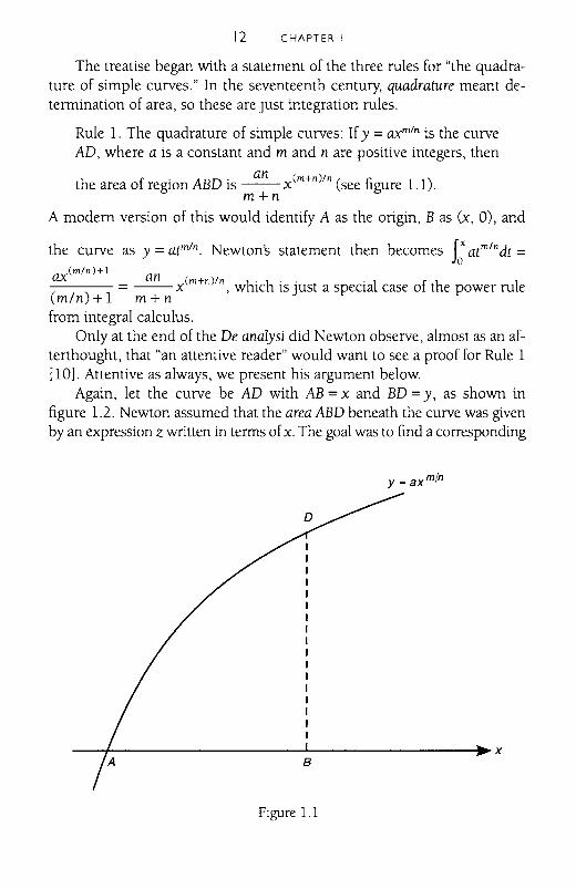
Rule 1. The quadrature of simple curves: If y =axm/n is the curveAD, where a is a constant and m and n are positive integers, then

an (m+n)/nthe area of region ABD is --x (see figure 1.1).

m+nA modern version of this would identify A as the origin, B as (x, 0), and

the curve as y =atm/n. Newton's statement then becomes f: atm/ndt =(m/n)+! a

ax n (m+nl/n h' h' . . 1 f h 1( ) =--x , W IC IS Just a specIa case 0 t e power ru emin + 1 m + n

from integral calculus.Only at the end of the De analysi did Newton observe, almost as an af­

terthought, that "an attentive reader" would want to see a proof for Rule 1[l0]. Attentive as always, we present his argument below.

Again, let the curve be AD with AB =x and BD =y, as shown infigure 1.2. Newton assumed that the area ABD beneath the curve was givenby an expression z written in terms of x. The goal was to find a corresponding

y = ax m/n

_---,/- ---I. ~. X

Figure 1.1

NEWTON 13

x

y

-_J HIIIIIIIIIVIIIIIIIII

-0-1

B fJ

Figure 1.2

formula for y in terms of x. From a modern vantage point, he was beginning

with z = J: y(t)dt and seeking y =y(x). His derivation blended geometry,

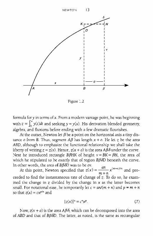
algebra, and fluxions before ending with a few dramatic flourishes.At the outset, Newton let f3 be a point on the horizontal axis a tiny dis­

tance 0 from B. Thus, segment Af3 has length x + o. He let z be the areaABD, although to emphasize the functional relationship we shall take theliberty of writing z =z(x). Hence, z(x + 0) is the area Af38 under the curve.Next he introduced rectangle Bf3HK of height v = BK = f3H, the area ofwhich he stipulated to be exactly that of region Bf35D beneath the curve.In other words, the area of Bf35D was to be OV. a

At this point, Newton specified that z(x) = __n_x(m+n)ln and pro-m+n

ceeded to find the instantaneous rate of change of z. To do so, he exam-ined the change in z divided by the change in x as the latter becomessmall. For notational ease, he temporarily let c =an/em + n) and p = m + n

so that z(x) =cxp1n and

(7)

Now, z(x + 0) is the area Af38, which can be decomposed into the areaof ABD and that of Bf35D. The latter, as noted, is the same as rectangular

14 CHAPTER I

area oy and so Newton concluded that z(x + 0) =z(x) + oy. Substitutinginto (7), he got

[z(x) + Oy]n = [z(x + o)]n = en(x + o)p,

and the binomials on the left and right were expanded to

[z(x)]n + n[z(x)]n-l oy + n(n -1) [z(x)]n-2 02y 2 + ...2

=enxp + enpxp-1o + en pep -1) Xp-202 + ....2

Applying (7) to cancel the leftmost terms on each side and then dividingthrough by 0, Newton arrived at

n[z(x)]n-I y + n(n -1) [Z(x)]n-2 0y2 + ...2

=enpxp- l + en pep -1) xp-20 + ...2

(8)

At that point, he wrote, "If we suppose Bf3 to be diminished infinitelyand to vanish, or 0 to be nothing, y and y in that case will be equal, and theterms which are multiplied by 0 will vanish" [11]. He was asserting that, as 0

becomes zero, so do all terms in (8) that contain o. At the same time, y becomesequal to y, which is to say that the height BK of the rectangle in Figure 1.2 willequal the ordinate BD of the original curve. In this way, (8) transforms into

(9)

A modern reader is likely to respond, "Not so fast, Isaac!" When New­ton divided by 0, that quantity most certainly was not zero. A momentlater, it was zero. There, in a nutshell, lay the rub. This zero/nonzero di­chotomy would trouble analysts for the next century and then some. Weshall have much more to say about this later in the book.

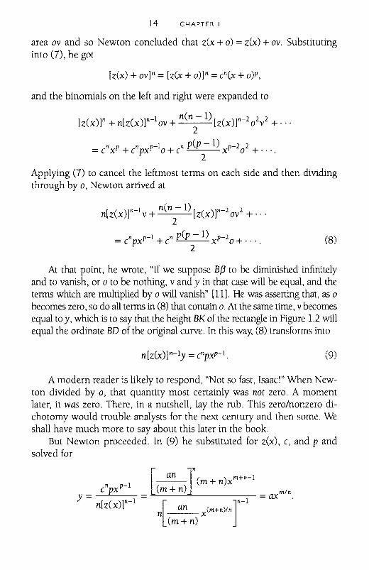
But Newton proceeded. In (9) he substituted for z(x), e, and p andsolved for

[an ]n (m + n)xm+n- 1

(m+n)=--__-=-- =ax m/ n

n[ an x<m+nvn]n-l(m+ n)

n p-le pxy = n[z(x)]n-l

NEWTON [5

Thus, starting from his assumption that the area ABD is given by

() an (m+n)lnZ x =--x . Newton had deduced that curve AD must satisfy the

m+nequation y =axm/n. He had, in essence, differentiated the integral. Then,without further justification, he stated, "Wherefore conversely, ifaxm/n =y,

it shall be~ x(m+n)/n = z." His proof of rule 1 was finished [12J.m+n

This was a peculiar tWlst of logic. HaVIng derived the equation ofy fromthat of its area accumulator z, Newton asserted that the relationship went

m/ an (m+n)/nthe other way and that the area under y =ax n is indeed --x .m+n

Such an argument tends to leave us with mixed feelings, for it featuressome gaping logical chasms. Derek Whiteside, editor of Newton's mathe­matical papers, aptly characterized this quadrature proof as "a brief,scarcely comprehensible appearance of fluxions" [13J. On the other hand,it is important to remember the source. Newton was writing at the verybeginning of the long calculus journey. Within the context of his time, theproof was groundbreaking, and his conclusion was correct. Somethingnngs true in RlChard Westfall's observation that, "however bnefly, De analysidid indicate the full extent and power of the fluXIonal method" [14].

Whatever the modern verdict, Newton was satisfied. His other tworules, for which the De analysi contained no proofs, were as follows:

Rule 2. The quadrature of curves compounded of simple ones: Ifthe value ofy be made up of several such terms, the area likewiseshall be made up of the areas which result from every one of theterms. [15J

Rule 3. The quadrature of all other curves: But if the value of y, orany of its terms be more compounded than the foregoing, it mustbe reduced into more simple terms ... and afterwards by the pre­ceding rules you Wlll discover the [areaJ of the curve sought. [16J

Newton's second rule affirmed that the integral of the sum of finitelymany terms is the sum of the integrals. This he illustrated Wlth an exampleor two. The third rule asserted that, when confronted with a more compli­cated expression, one was first to "reduce" it into an infinite series, integrateeach term of the senes by means of the first rule, and then sum the results.

This last was an appealing idea. More to the point, it was the final pre­requisite Newton would need to derive a mathematical blockbuster: theinfinite series for the sine of an angle. This great theorem from the Deanalysi will serve as the chapter's climax.

16 CHAPTER I

NEWTON'S DERIVATION OF THE SINE SERIES

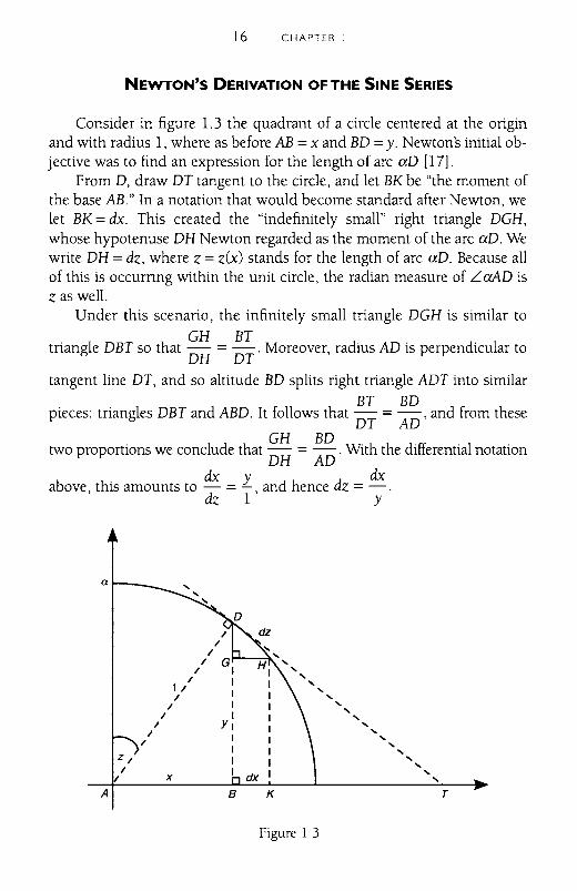
Consider in figure 1.3 the quadrant of a circle centered at the originand with radius 1, where as before AB =x and BD =y. Newton's initial ob­jective was to find an expression for the length of arc aD [17].

From D, draw DI tangent to the circle, and let BK be "the moment ofthe base AB." In a notation that would become standard after Newton, welet BK =dx. This created the "indefinitely small" right triangle DGH,whose hypotenuse DH Newton regarded as the moment of the arc aD. Wewrite DH = dz, where z = z(x) stands for the length of arc aD. Because allof this is occurnng within the unit circle, the radian measure of LaAD isz as well.

Under this scenario, the infinitely small triangle DGH is similar toGH BI

triangle DBI so that - =-. Moreover, radius AD is perpendicular toDH DI

tangent line DI, and so altitude BD splits right triangle ADI into similarBI BD

pieces: triangles DBI and ABD. It follows that DI = AD' and from these

GH BDtwo proportions we conclude that - =-. With the differential notation

DH ADdx y dx

above, this amounts to - = -, and hence dz = -.dz 1 Y

ar-__

//

//

//

1//

//

//

/

xB

" """ """ " " "" "" " "" " """K

Figure 13

T

NEWTON 17

Newton's next step was to exploit the circular relationship y = .J1 - x 2

dx dx 1to conclude that dz = - = ,-;--'f Expanding ,-;--'f as in (3) led to

y "l-x- "l-x-

dZ=[1+~X2+~x4+2x6+35 x8+ ...]dx2 8 16 128 '

and so

Ix IX [ 1 2 3 4 5 6 35 8 ]z=zex)= dz= l+-t +-t +-t +-t + ... dt.o 0 2 8 16 128

Finding the quadratures of these individual powers and summing the re­sults by Rule 3, Newton concluded that the arclength of aD was

1 3 3 5 5 7 35 9Z=x+-x +-x +-x +--x +... (0)6 40 112 1152

Referring again to Figure 1.3, we see that z is not only the radian mea­sure of LaAD, but the measure of LADB as well. From triangle ABD, weknow that sin Z =x and so

. 1 3 3 5 5 7 35 9arcsmx = Z =x+-x +-x +-x +--x + ....

6 40 112 1152

1

1 3 3 5 5 7--Z --Z --ZP = ----"6'-----_4"'-"0'-----~1"_"lo..=:2 _

1 2 3 4 5 6l+-z +-Z +-Z + ...2 8 16

18 CHAPTER [

1from which we retain only p = - - Z3. This extends the series to x =Z -

61 1"6 Z3. Next introduce p = -"6 Z3 + q and continue the inversion process,

solvmg for

1 5 1 7 1 8-Z +-Z --Z + ...

q = 120 56 721 2 3 4

l+-z +-Z + ...2 8

1 5 1 3 1 5or simply q =-- Z . At this stage x = Z - - Z +-- Z ,and, as Newton

120 6 120might say, we "continue at pleasure" until discerning the pattern and writ­ing down one of the most important series in analysis:

. 1 3 1 5 1 7 1 9sm Z = Z - - Z + -- Z - -- Z + Z _ ...6 120 5040 362880

00 k=L (-1) Z2k+l.

k=O (2k + I)!

B

0(

A

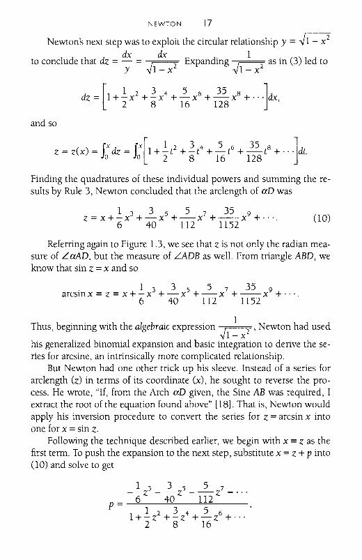
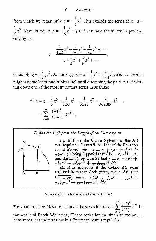
To find the Bafl: from the Length qf the Curve given.

45. If from the Arch aD given the Sine ABwas required; I extract the Root of the Equationfound above, viz. z.= X + {x1 + -lox> +I ~.X7 (it being fuppofed that AB = x, aD = z.and Aa= I) by which I find x=z -{z3 +_~Z5 - _1__Z 7 + I Z 9 &c110 50+0 J62.880 •

46. And moreover if the Coline A{3 wererequired from that Arch given, make A{3 (=../1 - xx) - I - _I z~ _L _I_Z + _ _~Z6 +- "'r,,, ... 710

4oT"i"oZS - T6-;FsooZ JO, &c.

Newton's series for sine and cosine (1669)

00 k~ (-1) 2k

For good measure, Newton included the series forcosz = £.. -(k)1 Z Ink=O 2 .

the words of Derek Whiteside, "These series for the sine and cosine ...here appear for the first time in a European manuscript" [19].

NEWTON 19

To us, this development seems incredibly roundabout. We now regardthe sine series as a trivial consequence of Taylor's formula and differentialcalculus. It is so natural a procedure that we expect it was always so. ButNewton, as we have seen, approached this very differently. He appliedrules of integration, not of differentiation; he generated the sine seriesfrom the (to our minds) incidental series for the arcsine; and he neededhis complicated inversion scheme to make it all work.

This episode reminds us that mathematics did not necessarily evolvein the manner of today's textbooks. Rather, it developed by fits and startsand odd surprises. Actually that is half the fun, for history is most intrigu­ing when it is at once Significant, beautiful, and unexpected.

On the subject of the unexpected, we add a word about Whiteside'squalification in the passage above. It seems that Newton was not the firstto discover a series for the sine. In 1545, the Indian mathematicianNilakantha (1445-1545) described this senes and credited it to his evenmore remote predecessor Madhava, who lived around 1400. An accountof these discoveries, and of the great Indian tradition in mathematics, canbe found in [20] and [21]. It is certain, however, that these results wereunknown in Europe when Newton was active.

We end with two observations. First, Newton's De ana/ysi is a trueclassic of mathematics, belonging on the bookshelf of anyone interested inhow calculus came to be. It provides a glimpse of one of history's most fer­tile thinkers at an early stage of his intellectual development.

Second, as should be evident by now, a revolution had begun. Theyoung Newton, with a skill and insight beyond his years, had combinedinfinite series and fluxional methods to push the frontiers of mathematicsin new directions. It was his contemporary, James Gregory (1638-1675),who observed that the elementary methods of the past bore the same rela­tionship to these new techniques "as dawn compares to the bright light ofnoon" [22]. Gregory's charming description was apt, as we see time andagain in the chapters to come. And first to travel down this exciting pathwas Isaac Newton, truly "a man of extraordinary genius and proficiency."

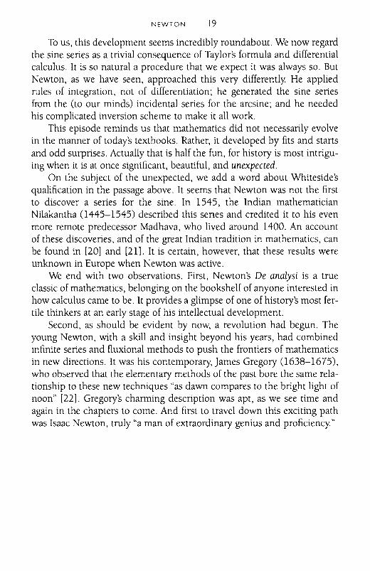
CHAPTER 2

Leibniz

Gottfried Wilhelm leibniz

Calculus may be unique in havmg as its founders two individualsbetter known for other things. In the public mind, Isaac Newton tends tobe regarded as a physicist, and his cocreator, Gottfried Wilhelm Leibniz(1646-1716), is likely to be thought of as a philosopher. This is bmhannoying and flattering-annoying in its disregard for their mathematicalcontributions and flattering in its recognition that it took more than Justan ordinary genius to launch the calculus.

Leibniz, with his vaned interests and far-reaching contributions, hadan intellect of phenomenal breadth. Besides philosophy and mathematics.he excelled in history, jurisprudence. languages, theology, logic, anddiplomacy. When only 27, he was admitted to Londons Royal Society forinventing a mechanical calculator that added, subtracted, multiplied, anddivided-a machine that was by all accounts as revolutionary as it wascomplicated [11.

20

LEIBNIZ 2 [

Like Newton, Leibniz had an intense penod of mathematical actiVIty,although his came later than Newton's and in a different country. WhereasNewton developed his fluxional ideas at Cambridge in the mid-1660s,Leibniz did his groundbreaking work while on a diplomatic mission toParis a decade later. This gave Newton temporal priority-which he andhis countrymen would later assert was the only kind that mattered-but itwas Leibniz who published his calculus at a time when the De analysi andother Newtonian treatises were gathering dust in manuscript form. Muchhas been written about the ensuing dispute over which of the twodeserved credit for the calculus, and the story is not a pretty one [2]. Mod­ern scholars, centuries removed from passions both national and personal,recognize that the discoveries of Newton and Leibniz were made indepen­dently Like an idea whose time had come, calculus was "in the air" andneeded only a remarkably penetrating and integrative mind to bring itinto existence. This Newton had.

Just as surely, so did Leibniz. Upon his arnval in Paris in 1672, he wasa nOVIce who admitted to lacking "the patience to read through the longseries of proofs" necessary for mathematical success [3]. Dissatisfied withhis modest knowledge, he spent time filling gaps, reading mathematiciansas venerable as Euclid (ca. 300 BeE) or as up-to-date as Pascal (1623-1662),Barrow, and his sometime-mentor, Chnstiaan Huygens (1629-1695). Atfirst it was hard going, but Leibniz persevered. He recalled that, in spite ofhis deficiencies, "it seemed to me, I do not know by what rash confidence inmy own ability, that I might become the equal of these if I so desired" [4].

Progress was breathtaking. He wrote in one memorable passage thatsoon he was "ready to get along without help, for I read [mathematics]almost as one reads tales of romance" [5]. After absorbing, almost inhaling,the work of his contemporaries, Leibniz pushed beyond them all to createthe calculus, thereby earning himself mathematical immortality

And, unlike Newton across the English Channel, Leibniz was willingto publish. The first pnnted version of the calculus was Leibnizs 1684 paperbearing the long title, "Nova methodus pro maximis et minimis, itemque tan­gentibus, quae nee fraetas, nee irrationales quantitates moratur; et singulare proillis calculi genus." This translates into "A New Method for Maxima andMinima, and also Tangents, which is Impeded Neither by Fractional Norby Irrational Quantities, and a Remarkable Type of Calculus for This" [6].With references to maxima, minima, and tangents, it should come as nosurprise that the article was Leibniz's introduction to differential calculus.He followed it two years later with a paper on integral calculus. Even atthat early stage, Leibniz not only had organized and codified many of the

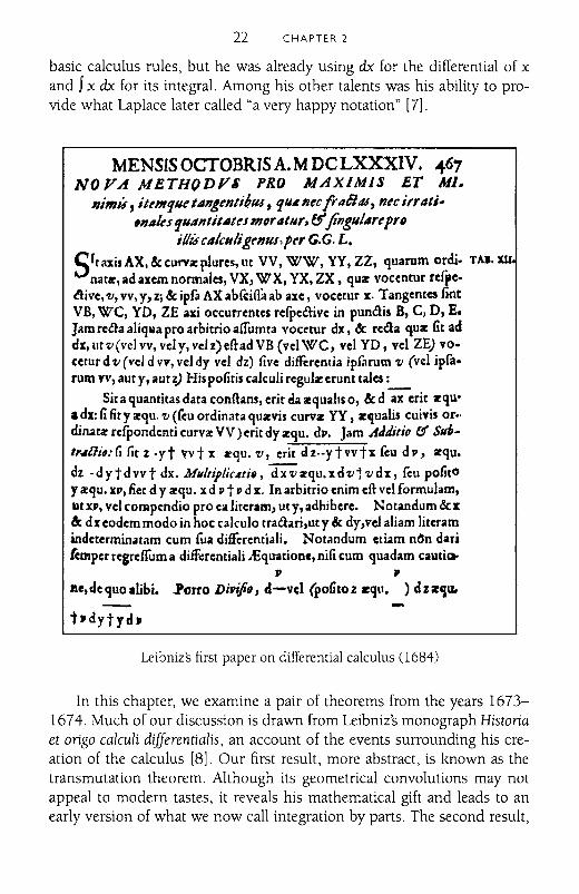
22 CHAPTER 2

basic calculus rules, but he was already using dx for the differential of xand Jx dx for its integral. Among his other talents was his ability to pro­vide what laplace later called "a very happy notation" [7].

MENSIS OcrOBRlSA. MDC LXXXIV. ....67NOPA METHQDPS PRO MAXIMIS ET MI.

ni1fJM, it~11I'jue tA1I!.entiQru, 'j'U n~cfrill/1M, 1Itcirrati­'lIala 'jUII1Ititiltn mOTatlir~ eIji1lgulareprtJ

HIMc"Ie"ligrnus,prr G.G. L.SftaxisAX,&curva:plures,llt VV, ww, yy,ZZ, quarum ordi. TAl. xu

natz, ad axem nonnales, VX, W X, YX, ZX, quz vocenrur refpe­c!tive, v, vv, y, z; &: ipfa AX abfltiifa ab axe, voc:etur x. Tangentes fHlt

VB, WC, YD, ZE axi occurrentes refped:ive in punClis B, C, 0 , E.J3m reela aliqNa pro arbitrio aifumta vocerur dx, &: rella quz ftt addx, lit v (vel vv, vel y, vel z) eftad VB (vel \'Q'C, vel YO, vel ZE) vo·eetur d v (vel d vv, vel dy vel dz) five differenfia ipfarum 'tI (vel ipfa.rum YV, aut y, aut z) His pofitis calculi regulz erunt tales :_

Sira quantitas data conftans, erit t'la zqualls 0, & d ax erit zqu'adx: li fity zqu. 'tI (feu ordinata quzvis curvz YY, zClualis cuiyis or··dinatz refpondenti curva: VV) erit dy zqu. dp. Jam AJditio £5 SIIb-t,....l1itJ:(i lit z ·yt yvt x zqu. v, erit dz·-ytvvtx feu dp, zqu.dz -dytdvvt dx. MliltiplieAti., ~zqu.xd'tltvdx, feu pofttO

y a:qu. XP, tiet d y zqu. xd P t p dx. In arbitrio enim eft vel formulam,ut X" vel compendio pro ea literam, ut y, adhibere. Notandum &: x&: dx eodem modo in hoc calculo trad:ari,ut y & dy,vel aliam literamindeterminatam cum fua differentiali. Notandum etiam nOn daritemper regrelfum a differentiali .Equation" nifi cum quadam cautio-

JI ,

ftC, de quo alibi. .Porro Di,ijo, d-vcl (poGto Z lIequ. ) dz z'lu,

tpdytyd,

Leibniz5 first paper on differential calculus (1684)

In this chapter, we examine a pair of theorems from the years 1673­1674. Much of our discussion is drawn from Leibniz's monograph Historiaet origo calculi differentialis, an account of the events surrounding his cre­ation of the calculus [8]. Our first result, more abstract, is known as thetransmutation theorem. Although its geometrical convolutions may notappeal to modern tastes, it reveals his mathematical gift and leads to anearly version of what we now call integration by parts. The second result,

LEIBNIZ 23

a consequence of the first, is the so-called "Leibniz Series." Like Newton'swork, discussed in the preVIous chapter, this combined series expansionsand basic integration techniques to produce an important and fascinatingoutcome.

THE TRANSMUTATION THEOREM

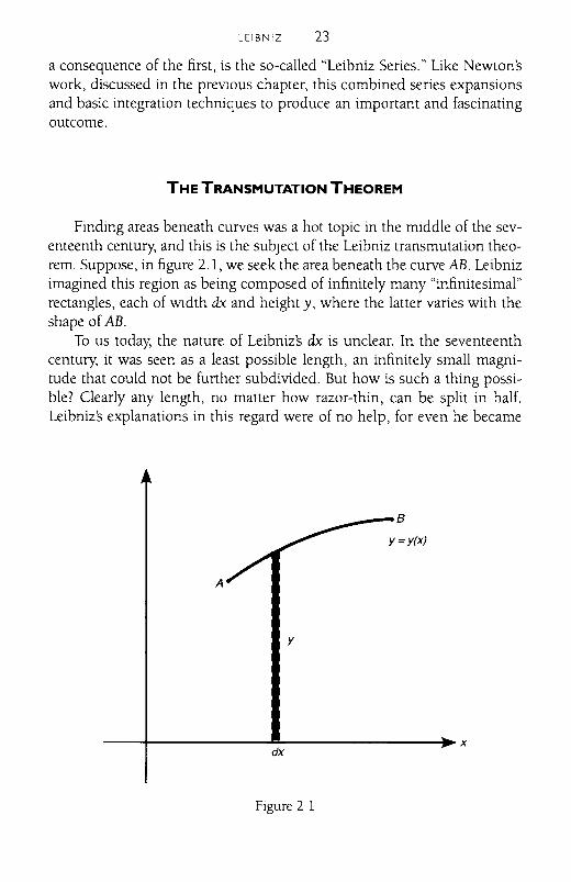
Finding areas beneath curves was a hot topic in the middle of the sev­enteenth century, and this is the subject of the Leibniz transmutation theo­rem. Suppose, in figure 2.1, we seek the area beneath the curve AB. Leibnizimagined this region as being composed of infinitely many "infinitesimal"rectangles, each of WIdth dx and height y, where the latter varies with theshape of AB.

To us today, the nature of Leibniz's dx is unclear. In the seventeenthcentury, it was seen as a least possible length, an infinitely small magni­tude that could not be further subdivided. But how is such a thing possi­ble? Clearly any length, no matter how razor-thin, can be split in half.Leibniz's explanations in this regard were of no help, for even he became

A

___-B

y=y(x)

y

---+-------~---------.. xdx

Figure 21

24 CHAPTER 2

unintelligible when addressing the matter. Consider the followmg passagefrom sometime after 1684:

by ... infinitely small, we understand something ... indefinitelysmall, so that each conducts itself as a sort of class, and not merelyas the last thing of a class. If anyone wishes to understand these[the infinitely small] as the ultimate things ... , it can be done,and that too WIthout falling back upon a controversy about thereality of extensions, or of infinite continuums in general, or ofthe infinitely small, ay even though he think that such things areutterly impossible. [9]

The reader is forgiven for finding this clarification less than clanfymg.Leibniz himself seemed to choose expediency over logic when he addedthat, even if the nature of these indivisibles is uncertain, they can nonethe­less be used as "a tool that has advantages for the purpose of the calcula­tion." Again we glimpse the mathematical quagmire that would confrontanalysts of the future. But in 1673 Leibniz was eager to press on, and alater generation could tidy up the logic.

Returning to figure 2.1, we see that the infinitesimal rectangle has areay dx. To calculate the area under the curve AB, Leibmz summed an infinitude

___-B

z

",

T ","'a",

W ",'"",4

",'" \\\h

\\

\\a

\\

ox

D11IIyIIIIII

dx

Figure 2 2

LEIBNIZ 25

of these areas. As a symbol for this process, he chose an elongated "s" (for"summa") and thus denoted the area as fy dx. Thereafter, his integral signbecame the "logo" of calculus, announcing to all who saw it that highermathematics was afoot.

It is one thing to have a notation for area and quite another to knowhow to compute it. Leibniz's transmutation theorem was aimed at resolv­ing this latter question.

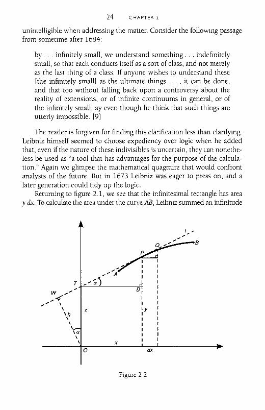
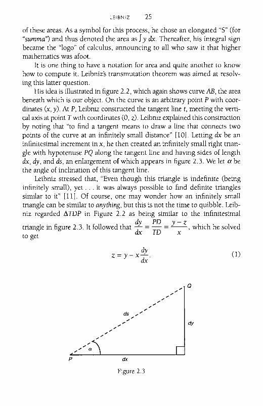
His idea is illustrated in figure 2.2, which again shows curve AB, the areabeneath which is our object. On the curve is an arbitrary point P with coor­dinates (x, y). At P, Leibmz constructed the tangent line t, meeting the verti­cal axis at point TWlth coordinates (0, z). Leibmz explained this constructionby noting that "to find a tangent means to draw a line that connects twopoints of the curve at an infinitely small distance" [10]. Letting dx be aninfinitesimal increment in x, he then created an infinitely small right tnan­gle with hypotenuse PQ along the tangent line and haVIng sides of lengthdx, dy, and ds, an enlargement of which appears in figure 2.3. We let ex bethe angle of inclination of this tangent line.

Leibniz stressed that, "Even though this triangle is indefinite (beinginfinitely small), yet ... it was always possible to find definite trianglessimilar to it" [11]. Of course, one may wonder how an infinitely smalltnangle can be similar to anything, but this is not the time to quibble. Leib­niz regarded tiTOP in Figure 2.2 as being similar to the infinitesimal

dy PO Y - ztriangle in figure 2.3. It followed that - = - =--, which he solvedto get dx TO x

p

dyz=y-x-.

dx

dx

Figure 2.3

Q

dy

(1)

26 CHAPTER 2

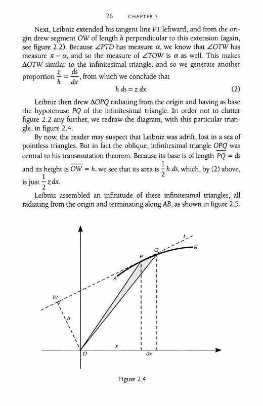
Next, Leibniz extended his tangent line PT leftward, and from the ori­gin drew segment OW of length h perpendicular to this extension (again,see figure 2.2). Because L.PTD has measure a, we know that LOTW hasmeasure 1r - a, and so the measure of LTOW is a as well. This makes.6.0TW similar to the infinitesimal triangle, and so we generate another

. z ds .propomon h= dx' from WhICh we conclude that

hds=zdx. (2)

Leibniz then drew .6.0PQ radiating from the origin and having as basethe hypotenuse PQ of the infinitesimal triangle. In order not to clutterfigure 2.2 any further, we redraw the diagram, with this particular trian­gle, in figure 2.4.

By now, the reader may suspect that Leibniz was adrift, lost in a sea ofpOintless triangles. But in fact the oblique, infinitesimal triangle OPQ was

central to his transmutation theorem. Because its base is of length PQ = ds~ 1

and its height is OW = h, we see that its area is -h ds, which, by (2) above,1 2

isjust-zdx.2

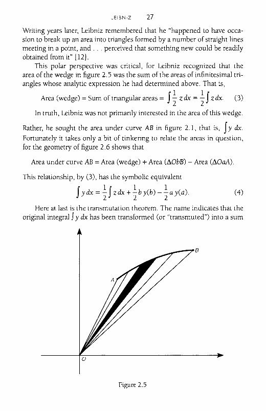
Leibniz assembled an infinitude of these infinitesimal triangles, allradiating from the ongin and terminating along AB, as shown in figure 2.5.

~_-B

x

w ,,4

-' ,,'h,,,,,,

o dx

Figure 2.4

(4)

LEIBNIZ 27

Writing years later, Leibniz remembered that he "happened to have occa­sion to break up an area into triangles formed by a number of straight linesmeeting in a point, and ... perceived that something new could be readilyobtained from it" [12J.

This polar perspective was critical, for Leibniz recognized that thearea of the wedge in figure 2.5 was the sum of the areas of infinitesimal tri­angles whose analytic expression he had determined above. That is,

Area (wedge) = Sum of tnangular areas = f1z dx = 1f z dx. (3)

In truth, Leibniz was not primanly interested in the area of this wedge.

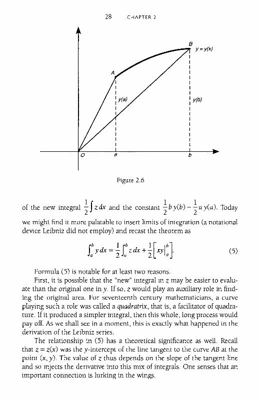
Rather, he sought the area under curve AB in figure 2.1, that is, fy dx.Fortunately it takes only a bit of tinkenng to relate the areas in question,for the geometry of figure 2.6 shows that

Area under curve AB =Area (wedge) + Area (~ObB) - Area (~OaA).

This relationship, by (3), has the symbolic equivalent

f ydx = ..!.fzdx +..!.b y(b) - ..!.ay(a).2 2 2

Here at last is the transmutation theorem. The name indicates that theoriginal integral f y dx has been transformed (or "transmuted") into a sum

~-7B

Figure 2.5

28 CHAPTER 2

B__-"1 Y =y(x)

11I11IIII y(b)II11III11

b

Figure 2.6

1f 1 1of the new integral "2 zdx and the constant "2 by(b) - "2 a yea). Today

we might find it more palatable to insert limits of integration (a notationaldeVlce Leibniz did not employ) and recast the theorem as

Jb 1 Jb 1[ bJydx = - zdx+- xyl .a 2 a 2 a

(5)

Formula (5) is notable for at least two reasons.First, it is possible that the "new" integral in z may be easier to evalu­

ate than the original one in y. If so, z would play an auxiliary role in find­ing the original area. For seventeenth century mathematiCians, a curveplaying such a role was called a quadratrix, that is, a facilitator of quadra­ture. If it produced a simpler integral, then this whole, long process wouldpayoff. As we shall see in a moment, this is exactly what happened in thederivation of the Leibniz series.

The relationship in (5) has a theoretical significance as well. Recallthat z =z(x) was the y-intercept of the line tangent to the curve AB at thepoint (x, y). The value of z thus depends on the slope of the tangent lineand so injects the derivative into this mix of integrals. One senses that animportant connection is lurking in the wings.

(6)

LEIBNIZ 29

dyTo see it, we recall from (1) that z = y - x- and so z dx =y dx - x dy.

Then, returning to (4), we have dx

f 1f 1 1ydx = - zdx + -b y(b) - -ay(a)2 2 2

I f I I= - [ydx - xdy] + -b y(b) - -ay(a)222

If If I I= - ydx-- xdy+-by(b)--ay(a)2 2 2 2 '

which we solve to conclude that fy dx =b y(b) - a yea) - fx dy.Again, limits of integration can be inserted to give

fb dx = X Ib

- fY(b) x da y y a y(a) y.

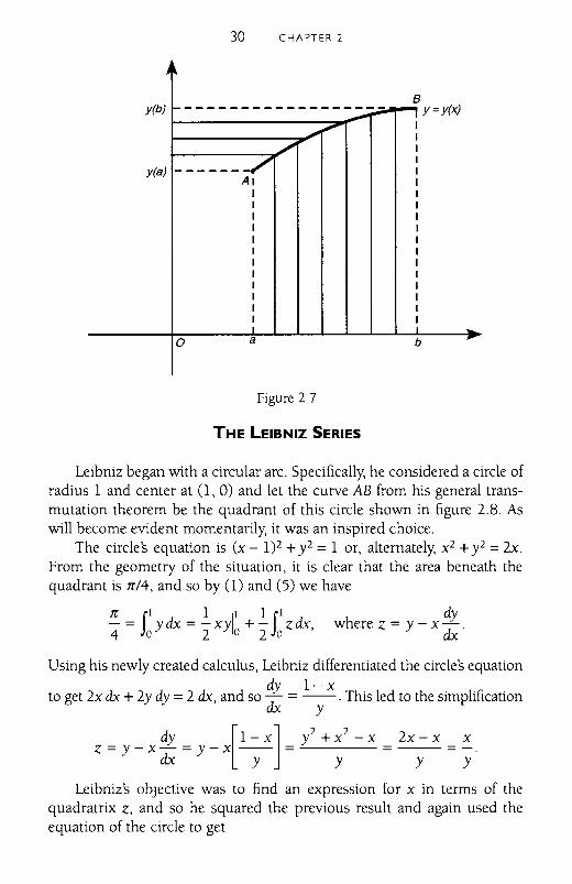
The geometric validity of (6) is evident in figure 2.7, for s: y dx is the

area of the region with vertical strips, whereas J;(~: x dy is the area of that

with horizontal strips. Their sum is clearly the difference in area betweenthe outer rectangle and the small one in the lower left-hand corner. That is,

fb fY(b)ydx+ xdy=by(b)-ay(a),a y(a)

which can be rearranged into (6).There is something else about (6) that bears comment: it looks famil­

iar. So it should, because it follows easily from the well-known scheme forintegration by parts

f: f(x)g'(x)dx = f(x) g(x)l: - f: g(x) j'(x)dx,

if we specify g(x) = x and f(x) = y. In that case g'(x) = 1 and j'(x)dx = dy,and a substitution converts the integration-by-parts formula into thetransmutation theorem. After all of Leibniz's convoluted reasoning with itsinfinitesimals and tangent lines, its similar triangles and wedge-shapedareas-in short, after a most circuitous mathematical Journey-we arrive atan instance of integration by parts, a calculus superstar making an early andunexpected entrance onto the stage.

This was intriguing, but Leibniz was not finished. By applying his trans­mutation theorem to a well-known curve, he discovered the infinite senesthat still carries his name.

30 CHAPTER 2

-'I'

By(b) ~------------------ -, y=y(x)--

~"'"II

/ I

------7/I

y(a) IAI I

IIIIIIIIIIII

0 a b,

Figure 2 7

THE LEIBNIZ SERIES

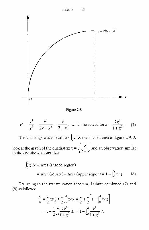
Leibniz began with a circular arc. Specifically, he considered a circle ofradius 1 and center at (1, 0) and let the curve AB from his general trans­mutation theorem be the quadrant of this circle shown in figure 2.8. Aswill become evident momentarily, it was an inspired choice.

The circle's equation is (x - 1)2 + y2 = lor, alternately, x2+ y2 = 2x.From the geometry of the situation, it is clear that the area beneath thequadrant is n/4, and so by (1) and (5) we have

n 11 1 II 1 11 dy- = Ydx = - x y + - zdx where z = y - x -.4 ° 2 ° 20 ' dx

Using his newly created calculus, Leibniz differentiated the circles equationdy 1- x

to get 2x dx + 2y dy =2 dx, and so dx = -y-' This led to the simplification

Z= Y - x~ = Y _ f ~ x ] = y' +:' -x = 2X; x = ~

Leibniz's objective was to find an expression for x in terms of thequadratrix z, and so he squared the previous result and again used theequation of the circle to get

LEIBNIZ 31

y=V2x-x2

a

Figure 2 8

2 X2

X2

X 2Z 2

Z = - =--~ = which he solved for x = --2 .l 2x - x 2 2 - x ' 1+ z

x

(7)

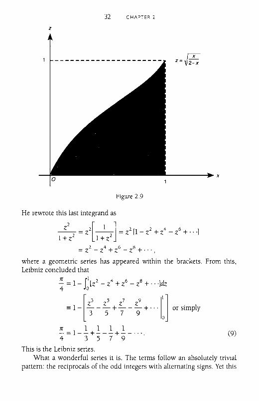
The challenge was to evaluate J>dx, the shaded area in figure 2.9. A

look at the graph of the quadratrix z =~ x and an observation similar2-xto the one above shows that

J~ zdx = Area (shaded region)

= Area (square) - Area (upper region) = 1 - f~ x dz. (8)

Returning to the transmutation theorem, Leibniz combined (7) and(8) as follows:

nIl 1 11 1 1 [ 11 ]- = - xyl + - z dx = - + - 1 - x dz4 2 020 22 0

1II 2z2 11 Z2=1-- --dz =1- --dz.

2 0 1+ Z2 0 1+ Z2

32 CHAPTER 2

z

o

Figure 2.9

z= J2~X

L...-----...... X

He rewrote this last integrand as

Z2 2[ 1] 2 2 4 6-- = z -- = z [1- z + z - z + 0 0 oj1+ Z2 1+ Z2

= Z2 _ Z4 + Z6 - Z8 + . 0 0 ,

where a geometric series has appeared within the brackets. From this,Leibniz concluded that

!!.- =1- rl [z2 - Z4 + Z6 - Z8 + 0 0 ojdz4 Jo

=1- [ ; <<<+.. :J or simply

7C 1 1 1 1- = 1 - - + - - - + - - .. o. (9)4 3 5 7 9

This is the Leibniz series.What a wonderful series it is. The terms follow an absolutely triVIal

pattern: the reciprocals of the odd integers with alternating signs. Yet this

LEIBNIZ 33lC

innocuous-looking expression sums to, of all things, 4 Leibniz recalled

that when he first communicated the result to Huygens, he received ravereviews, for "the latter praised it very highly, and when he returned thedissertation said, in the letter that accompanied it, that it would be a dis­covery always to be remembered among mathematicians" [13].

The significance of this discovery, according to Leibniz, was that "itwas now proved for the first time that the area of a circle was exactly equalto a senes of rational quantities" [14]. One may quibble with his use of"exactly," but it is hard to argue WIth his enthusiasm.

He added a curious postscript. By dividing each side of (9) in half andgrouping the terms, Leibniz saw that

~ = (±-i) +C~ -1~ ) +C~ -212) + (2

16 - 3

10) + ...

1 1 1 1=-+-+-+-+ ...3 35 99 195

1 1 1 1=--+--+ + + ...22

- 1 62- 1 102

- 1 142- 1 .

In words, this says that if we diminish by 1 the square of every other evenlC

number starting with 2 and then add the reciprocals, the sum is -. How8

strange. One is reminded that formulas from analysis can border on themagical.

The Leibniz series, remarkable as it is, has no value as a numericalapproximator of lC The series converges, but it does so with excruciatingslowness. One could add the first 300 terms of the Leibniz series and stillhave lC accurate to only a single decimal place. Such dreadful precisionwould not be worth the effort. However, as we shall see, a related infinitesenes would, in the hands of Euler, produce a highly efficient scheme forapproximating lC.

Unquestionably, the Leibniz series is a calculus masterpiece. As is cus­tomary when discussing these early results, however, we must offer a fewwords of caution. For one thing, the transmutation theorem used infinitesi­mal reasoning. For another, evaluating his senes required Leibniz to replacethe integral of an infinite sum by the sum of infinitely many integrals, a pro­cedure whose subtleties would be addressed in the centuries to come.

And there was one other problem: Leibniz was not the first to discoverthis series. The British mathematician James Gregory had found something

34 CHAPTER 2

very similar a few years before. Gregory had, in fact, come upon an expan­sion for arctangent, namely,

x 3X

5 x7

arctan x = x - - + - - - + ...3 5 7 '

which, for x = 1, is the Leibniz series (although Gregory may never haveactually made the substitution to convert this to a series of numbers).

Leibniz, a mathematical novice in 1674, was unaware of Gregoryswork and believed he had hit upon something new. This in turn led hisBritish counterparts to regard him with some suspicion. To them, Leibnizhad a tendency to claim credit for the achievements of others. These suspi­cions, of course, would be magnified early in the eighteenth century whenthe British, under the direction of Newton himself, accused Leibniz of out­right plagiarism in stealing the calculus. The confusion over the series

1r 1 1 1 1- = 1 - - + - - - + - - ... was seen as an early instance of Leibnizs43579

perfidy.But even Gregory was not the first down this path. The Indian mathe­

matician Nilakantha, whom we met in the preVIOUS chapter, described thisseries-in verse, no less-in a work called the Tantrasangraha [15].Although it was unknown in Europe during Leibnizs day, this achievementserves as a reminder that mathematics is a universal human enterprise.

The work of Gregory and Nilakantha nothwithstanding, we know thatLeibnizs derivation of this series was not theft. He later wrote that in 1674neither he nor Huygens "nor yet anyone else in Paris had heard anythingat all by report concerning the expression of the area of a circle by meansof an infinite series of rationals" [16]. The Leibniz series, like the calculusgenerally, was a personal triumph.

Over the next two decades, the nOVIce would become the master asLeibniz refined, codified, and published his ideas on differential and inte­gral calculus. From such beginnings, the subject would grow-indeed,would explode-in the century to come. We continue this story WIth alook at his two most distinguished followers, the Bernoulli brothers ofSWItzerland.

CHAPTER J

The Bernoullis

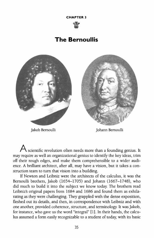
Jakob Bernoulli Johann Bernoulli

Ascientific revolution often needs more than a founding genius. Itmay require as well an organizational genius to identify the key ideas, trimoff their rough edges, and make them comprehensible to a wider audi­ence. A bnlliant architect, after all, may have a vision, but it takes a con­struction team to turn that vision into a building.

If Newton and Leibniz were the architects of the calculus, it was theBernoulli brothers, Jakob (1654-1705) and Johann (1667-1748), whodid much to build it into the subject we know today. The brothers readLeibniz's original papers from 1684 and 1686 and found them as exhila­rating as they were challenging. They grappled Wlth the dense exposition,fleshed out its details, and then, in correspondence with Leibniz and withone another, provided coherence, structure, and terminology. It was jakob,for instance, who gave us the word "integral" 11). In their hands, the calcu­lus assumed a form easily recognizable to a student of today, with its basic

35

36 CHAPTER 3

rules of derivatives, techniques of integration, and solutions of elementarydifferential equations.

Although excellent mathematicians, the Bernoulli brothers exhibited apersonal behavIOr best described as "unbecoming." Johann, in particular,assumed the combative role of Leibniz:S bulldog in the calculus wars WlthNewton, remaining loyal to his hero, whom he called the "celebrated Leib­niz," and going so far as to suggest that not only did Newton fail to inventcalculus but he never completely understood it [2]! This was certainly abrazen attack on one of history's greatest mathematicians.

Unfortunately for family harmony, Jakob and Johann were only toohappy to do battle with one another. Older brother Jakob, for instance,would refer to Johann as "my pupil," even when the pupil's talents wereclearly equal to his own. And, decades after the fact, Johann gleefullyrecalled solving in a single night a problem that had stumped Jakob for thebetter part of a year [3].

Their difficult natures notwithstanding, the Bernoullis left deep foot­prints. Besides his contributions to calculus, Jakob wrote the Ars conjectan­di, posthumously published in 1713. This work is a classic of probabilitytheory that features a proof of the law of large numbers, a fundamentalresult that it is sometimes called "Bernoulli's theorem" in his honor [4].For his part, Johann was the ghostwriter of the world's first calculus text.This came to pass because of an agreement to supply calculus lessons, fora fee, to a French nobleman, the Marquis de l'Hospital 0661-1704).L'Hospital, in turn, assembled and published these in 1696 under thetitle Analyse des infiniment petits pour l'intelligence des /ignes courbes (Analy­sis of the Infinitely Small for the Understanding of Curved Lines). In thiswork first appeared "l'Hospital's rule," a fixture of differential calculus eversince, although it, like so much of the book, was actually Johann Bernoul­li's [5]. In the preface, l'Hospital acknowledged his debt to Bernoulli andLeibniz when he wrote, "I have made free use of their discoveries so that Ifrankly return to them whatever they please to claim as their own" [6].

The irascible Johann, who indeed claimed the rule, was not satisfiedwith this gesture and in later years grumbled that l'Hospital had cashed inon the talents of others. Of course it was Bernoulli who (literally) did thecashing in, as math historian Dirk Struik reminded us Wlth this succinct rec­ommendation: "Let the good Marquis keep his elegant rule; he paid for it"[7]. To avoid losing glory a second time, Johann wrote an extensive treatiseon integral calculus that was published, under his own name, in 1742 [8].

To get a clearer sense of their mathematical achievements, we shall con­sider selected works from each brother. We begin Wlth Jakob:S divergenceproof of the harmonic series, then examine his treatment of some curious

THE BERNOULLIS 37

convergent series, and conclude with Johann's contnbutions to what hecalled the "exponential calculus."

JAKOB AND THE HARMONIC SERIES

Like Newton and Leibniz before him-and so many afterward-JakobBernoulli regarded infinite senes as a natural pathway into analysis. Thiswas eVIdent in his 1689 work, Tractatus de seriebus infinitis earumque summafinita (Treatise on Infinite Senes and Their Finite Sums), a state-of-the-artdiscussion of infinite senes as they were understood near the end of theseventeenth century [9]. Jakob considered such familiar series as the geo­metnc, binomial, arctangent, and logarithmic, as well as some previouslyunexamined ones. In this chapter, we look at two excerpts from the Tracta­tus, the first of which addressed the strange behavior of the harmonicseries.

1 1 1Long before 1689, others had recognized that 1+ - + - + - + ...

234diverges to infinity. Nicole Oresme (ca. 1323-1382) deVIsed the prooffound in most modern texts, and Pietro Mengoli 0625-1686) came upWIth an alternate demonstration in 1650 [10]. Leibniz, perhaps unaware ofthese predecessors, discovered divergence during his early Pans years and

1 1 1 1informed his Bntish contacts that, in his words, 1+ - + - + - + ... = -,

2 3 4 0only to learn from them that he had been scooped once again [11].

So, the divergence of the harmonic series was hardly news. But wemay gain insight, not to mention the charm of variety, by folloWIng alter­nate routes to the same end. Jakob Bernoulli's divergence proof, quite dif­ferent from those of his predecessors, is such an alternative.

He began by comparing two types of progressions that held centerstage in his day: the geometric and the arithmetic. The former hedescribed as A, B, C, D, ... , where BIA = C/B = DIC, etc., for example, 2,1, 1/2, 1/4, .... The latter, he wrote, had the form A, B, C, D, ... , whereB- A =C - B=D - C, etc.; an example is 2, 5, 8, 11, .... The modernconvention, of course, is to emphasize the common ratio (r) in geometricprogressions and the common difference (d) in arithmetic ones, so that wedenote a geometric progression by A, Ar, Ar2 , Ar3 ... and an arithmeticone by A, A + d, A + 2d, A + 3d ....

As the fourth proposition of his Tractatus, Jakob proved a lemmaabout geometnc and arithmetic progressions of positive numbers thatbegin WIth the same first two terms.

38 CHAPTER 3

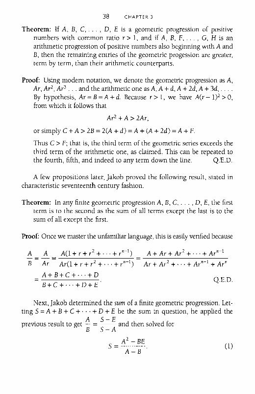
Theorem: If A, B, C, ... , D, E is a geometric progression of positivenumbers with common ratio r> 1, and if A, B, F, ... , G, H is anarithmetic progression of positive numbers also beginning WIth A andB, then the remaining entries of the geometric progession are greater,term by term, than their arithmetic counterparts.

Proof: Using modern notation, we denote the geometric progression as A,Ar, Ar2 , Ar3 ... and the arithmetic one as A, A + d, A + 2d, A + 3d, ....By hypothesis, Ar =B=A + d. Because r> 1, we have A(r - 1)2 > 0,from which it follows that

Ar2 + A> 2Ar,

or simply C + A> 2B = 2(A + d) =A + (A + 2d) =A + F.

Thus C> F; that is, the third term of the geometric series exceeds thethird term of the arithmetic one, as claimed. This can be repeated tothe fourth, fifth, and indeed to any term down the line. Q.E.D.

A few propositions later, Jakob proved the following result, stated incharacteristic seventeenth century fashion.

Theorem: In any finite geometric progression A, B, C, ... , D, E, the firstterm is to the second as the sum of all terms except the last is to thesum of all except the first.

Proof: Once we master the unfamiliar language, this is easily venfied because

A

B

A A(1+r+r2 +···+rn-

l)

=----------Ar Ar(l + r + r 2 + ... + rn

-l)

A+B+C+ .. ·+D

B+C+···+D+E

A+ Ar+ Ar2 + ... + Arn-

l

Ar + Ar2 + ... + Arn-

l + Arn

Q.E.D.

Next, Jakob determined the sum of a finite geometric progression. Let­ting 5 =A + B + C + ... + D + E be the sum in question, he applied the

A S-Eprevious result to get - =-- and then solved for

B S-A

A2 -BE5=--­

A-B(1)

THE BERNOULLIS 39

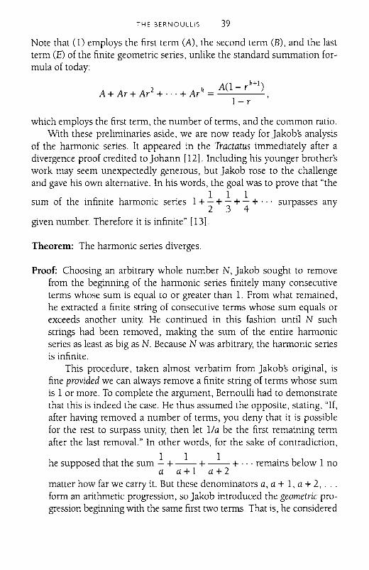
Note that (I) employs the first term (A), the second term (B), and the lastterm (E) of the finite geometric series, unlike the standard summation for­mula of today:

2 k A(l-rk+

1)

A+Ar+Ar +···+Ar =---­1- r '

which employs the first term, the number of terms, and the common ratio.With these preliminaries aside, we are now ready for Jakob's analysis

of the harmonic series. It appeared in the Tractatus immediately after adivergence proof credited to Johann [12]. Including his younger brother'swork may seem unexpectedly generous, but Jakob rose to the challengeand gave his own alternative. In his words, the goal was to prove that "the

I I Isum of the infinite harmonic series I + - + - + - + . .. surpasses any

234given number. Therefore it is infinite" [13].

Theorem: The harmonic series diverges.

Proof: Choosing an arbitrary whole number N, Jakob sought to removefrom the beginning of the harmonic series finitely many consecutiveterms whose sum is equal to or greater than 1. From what remained,he extracted a finite string of consecutive terms whose sum equals orexceeds another unity. He continued in this fashion until N suchstrings had been removed, making the sum of the entire harmonicseries as least as big as N. Because N was arbitrary, the harmonic seriesis infinite.

This procedure, taken almost verbatim from Jakob's original, isfine provided we can always remove a finite string of terms whose sumis I or more. To complete the argument, Bernoulli had to demonstratethat this is indeed the case. He thus assumed the opposite, stating, "If,after having removed a number of terms, you deny that it is possiblefor the rest to surpass unity, then let 11a be the first remaining termafter the last removal." In other words, for the sake of contradiction,

he supposed that the sum.!. + _1_ + _1_ + ... remains below I noa a+1 a+2

matter how far we carry it. But these denominators a, a + I, a + 2, ...form an arithmetic progression, so Jakob introduced the geometric pro­gression beginning with the same first two terms. That is, he considered

40 CHAPTER 3

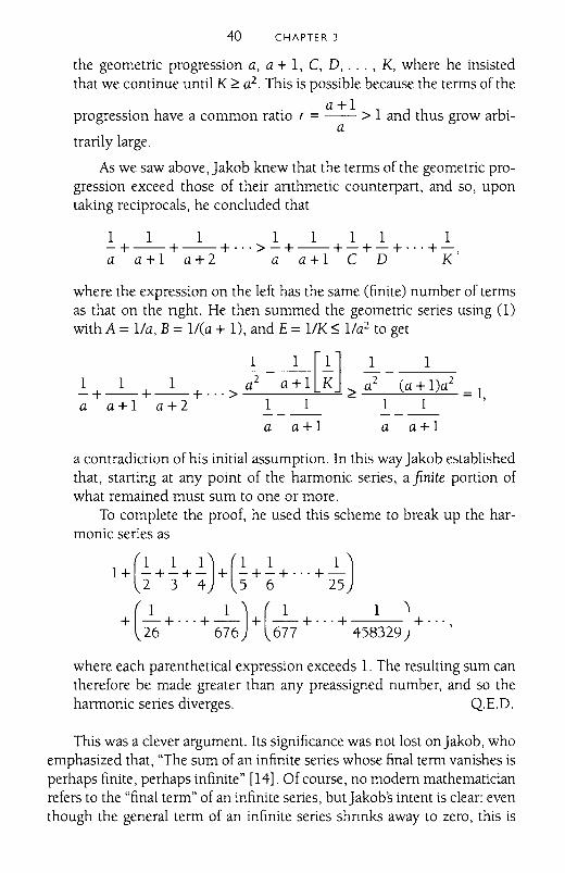
the geometric progression a, a + 1, C, D, ... , K, where he insistedthat we continue until K ~ a2 . This is possible because the terms of the

a+lprogression have a common ratio r =-- > 1 and thus grow arbi­

atrarily large.

As we saw above, Jakob knew that the terms of the geometric pro­gression exceed those of their anthmetic counterpart, and so, upontaking reciprocals, he concluded that

11 1 1111 1-+--+--+ ... > -+--+-+-+ ... +-a a+l a+2 a a+l C D K'

where the expression on the left has the same (finite) number of termsas that on the nght. He then summed the geometric series using (1)with A = lla, B= I/(a + 1), and E = 11K::; l1a2 to get

a a +1 a a + 1

a contradiction of his initial assumption. In this way Jakob establishedthat, starting at any point of the harmonic series, a finite portion ofwhat remained must sum to one or more.

To complete the proof, he used this scheme to break up the har­monic series as

1+(~ +~ + ~) + (.!. +~ + ... +~)2 3 4 5 6 25

+(_1 + ... +_1)+(_1 + ... + 1 )+ ...26 676 677 458329 '

where each parenthetical expression exceeds 1. The resulting sum cantherefore be made greater than any preassigned number, and so theharmonic series diverges. Q.E.D.

This was a clever argument. Its significance was not lost on Jakob, whoemphasized that, "The sum of an infinite series whose final term vanishes isperhaps finite, perhaps infinite" [14]. Of course, no modern mathematicianrefers to the "final term" of an infinite series, butJakobs intent is clear: eventhough the general term of an infinite series shnnks away to zero, this is

THE BERNOULLIS 41

not sufficient to guarantee convergence. The harmonic series stands as thegreat example to illustrate this point. So it was for Jakob Bernoulli, and soit remains today

JAKOB AND HIS FIGURATE SERIES

The harmonic series was of interest because of its bad, that is, diver­gent, behavior. Of equal interest were well-behaved infinite series havingfinite sums. Starting with the geometric senes and cleverly modifYIng theoutcome, Jakob proceeded until he could calculate the exact values ofsome nontrivial series. We consider a few of these below.

First he needed the sum of an infinite geometric progression. As notedin (1), Bernoulli summed a finite geometric series with the formula

A 2- BE

A+B+C+···+D+E=---A-B

As a corollary he observed that, for an infinite geometric progression ofpositive terms whose common ratio is less than 1, the general term mustapproach zero So he simply let his "last" term E =0 to arrive at

A2

A + B+ C + ... + D + ... =-- (2)A-B

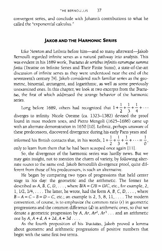
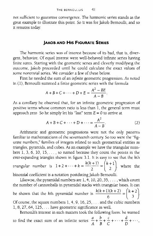
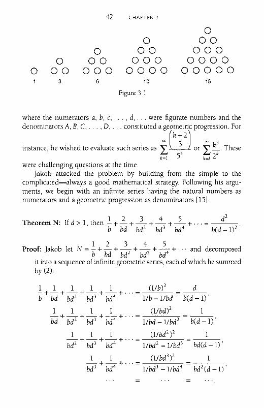
Arithmetic and geometnc progressions were not the only patternsfamiliar to mathematicians of the seventeenth century. So too were the "fig­urate numbers," families of integers related to such geometrical entities astriangles, pyramids, and cubes. As an example we have the triangular num­bers 1, 3, 6, 10, 15, ... , so named because they count the points in theever-expanding triangles shown in figure 3.1. It is easy to see that the kth

k(k + 1) (k + 1)tnangular number is 1+ 2 + ... + k = 2 = 2 ' where the

binomial coefficient is a notation postdating Jakob Bernoulli.likeWIse, the pyramidal numbers are 1,4,10,20,35, ... , which count

the number of cannonballs in pyramidal stacks with tnangular bases. It can

. k(k + 1)(k + 2) (k + 2)be shown that the kth pyramIdal number is 6 = 3 .

Of course, the square numbers 1,4,9, 16,25, ... and the cubic numbers1,8,27,64, 125, ... have geometric significance as well.

Bernoulli's interest in such matters took the follOwing form: he wantedabc d

to find the exact sum of an infinite series - + - + - + ... + - + ...ABC D '

42 CHAPTER 3

00 00

0 00 0000 00 000 0000

0 00 000 0000 000003 6 10 15

Figure 3 1

where the numerators a, b, c, , d, ... were figurate numbers and the

denominators A, B, C, ... , D, constituted a~e(o~;t~)'c pro~es:ion. For

instance, he wished to evaluate such series as I k or I ;. Thesek=! 5 k=! 2

were challenging questions at the time.Jakob attacked the problem by building from the simple to the

complicated-always a good mathematical strategy. Following his argu­ments, we begin with an infinite series having the natural numbers asnumerators and a geometric progression as denominators [15].

1 2 3 4 5 d2

Theorem N: If d > 1, then - + - + - + - + - + ... = .b bd bd2 bd3 bd4 bed - Ii

1 2 3 4 5Proof: Jakob let N = - + - + - + - + - + . .. and decomposed

b bd bd2 bd3 bd4

it into a sequence of infinite geometric senes, each of which he summedby (2):

1 1 1 1 1 (llb)2 d-+-+-+-+-+ ... = =---b bd bd2 bd3 bd4 lib - l/bd bed - 1) ,

1 1 1 1 (llbdi 1-+-+-+-+ ... = =---bd bd2 bd3 bd4 Ilbd - I1bd 2 bed - 1) ,

1 1 1 (llbd 2)2 1-+-+-+ ... = =---bd2 bd3 bd4 I1bd 2 - I1bd 3 bd(d - 1) ,

1 1 (llbd 3 i 1-+-+ ... = =-:----bd3 bd4 I1bd 3

- I1bd 4 bd2(d - 1) ,

= =

THE BERNOULLIS 43

Upon adding down the columns, he found

1 2 3 4 5N = -+-+-+-+-+ ...

b bd bd 2 bd 3 bd4

d 1 1 1= + + + + ...bed -1) bed -1) bd(d -1) bd2 (d -1)

= d ~ 1[~+ :d +~2 +b~3 +.. ]= d ~ 1[ lib~~d ]

d2

=---bed _1)2 '

because the infinite series in brackets is again geometric. Q.E.D.

..2345For mstance, WIth b =1 and d =7, we have 1+ - + - + - +-- + ...

72 49 7 49 343 2401=--=-

1x 62 36

Next, Jakob put triangular numbers in the numerators.

Theorem T: If d > 1, then

d3

bed _1)3 .

1 3 6 10 15T:=-+-+-+-+-+···=

b bd bd 2 bd 3 bd 4

Proof: The trick is to break T into a string of geometric series and exploitthe fact that the kth triangular number is 1 + 2 + 3 + ... + k:

1 1 1 1 1 (llb)2 d-+-+-+-+-+ ... = =---b bd bd2 bd3 bd4 lib - Ilbd bed - 1) ,

2 2 2 2 (2lbdi 2-+-+-+-+ ... = =---bd bd 2 bd3 bd4 21bd - 21bd2 bed - 1) ,

3 3 3 C3lbd2 i 3-+-+-+ ... = =---bd2 bd3 bd4 31bd2

- 31bd3 bd(d -1) ,

4 4 (4lbd 3 i 4-+-+ ... = =----bd3 bd4 41bd3

- 41bd 4 bd 2 (d - 1) ,

= =

44 CHAPTER 3

Adding down the columns gives

1 1+2 1+2+3 1+2+3+4-+--+ + + ...b bd bd 2 bd3

d 2 3 4= + + + + ....bed -1) bed - 1) bd(d - 1) bd 2 (d - 1)

In other words,

T = _d_ [.!. +~ + -.2..- + ---±- + ...Jd - 1 b bd bd 2 bd3

d d d2 d3

=--N=--x =---d - 1 d - 1 bed - Ii bed _1)3 '

Q.E.D.

1 3 6 10 15-+-+-+-+-+2 8 32 128 512

by theorem N.

For example, WIth b = 2 and d = 4, we have32

27

Jakob then considered pyramidal numbers in the numerators.

1 4 10 20 35Theorem P: If d > 1 x then P == - + - + - + - + - + ... =

, b bd bd 2 bd3 bd4

d4

bed - 1)4 .

Proof: This follows easily because

Hence (1 - .!.Jp = T = d3

and so P = __d_4

_d bed - 1)3 ' bed - 1)4 .

As an example, with b = 5 and d = 5, we have

Q.E.D.

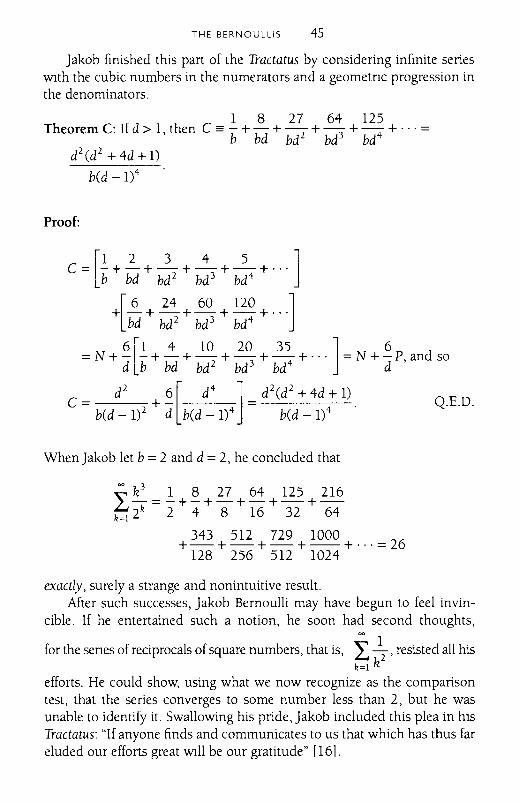
THE BERNOULLIS 45

Jakob finished this part of the Tractatus by considering infinite seriesWIth the cubic numbers in the numerators and a geometnc progression inthe denominators.

1 8 27 64 125Theorem C: If d > 1 then C = -+-+-+-+-+ ... =

, b bd bd 2 bd 3 bd 4

d2 Cd 2 + 4d + 1)

bCd _1)4

Proof:

When Jakob let b= 2 and d = 2, he concluded that

i £ = ~ +~ + 27 + 64 + 125 + 216k=! 2k 2 4 8 16 32 64

+ 343 + 512 + 729 + 1000 + ... = 26128 256 512 1024

exactly, surely a strange and nonintuitive result.After such successes, Jakob Bernoulli may have begun to feel invin­

cible. If he entertained such a notion, he soon had second thoughts,

for the senes of reciprocals of square numbers, that is, i ~, resisted all hisk=! k

efforts. He could show, using what we now recognize as the comparisontest, that the series converges to some number less than 2, but he wasunable to identify it. Swallowing his pride, Jakob included this plea in hisTractatus: "If anyone finds and communicates to us that which has thus fareluded our efforts great WIll be our gratitude" [16].

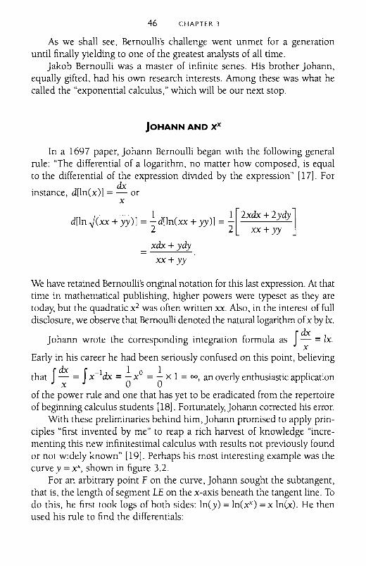
46 CHAPTER 3

As we shall see, Bernoulli's challenge went unmet for a generationuntil finally yielding to one of the greatest analysts of all time.

Jakob Bernoulli was a master of infinite senes. His brother Johann,equally gifted, had his own research interests. Among these was what hecalled the "exponential calculus," which will be our next stop.

JOHANN AND XX

In a 1697 paper, Johann Bernoulli began WIth the following generalrule: "The differential of a logarithm, no matter how composed, is equalto the differential of the expression diVIded by the expression" [17]. For

instance, d[ln(x)] = dx orx

d[ln ~(xx + yy)] = ~d[ln(xx + yy)] = ~[2Xdx + 2YdY]2 2 xx + yy

xdx+ ydy=-_....=....-.=....xx+ yy

We have retained Bernoullis onginal notation for this last expression. At thattime in mathematical publishing, higher powers were typeset as they aretoday, but the quadratic x2 was often written xx. Also, in the interest of fulldisclosure, we observe that Bernoulli denoted the natural logarithm ofx by Ix.

Johann wrote the corresponding integration formula as Jdx = Ix.x

Early in his career he had been seriously confused on this point, believing

Jdx J- 1 1that - = x ldx = - XO = - x 1 = 00, an overly enthusiastic applicationx 0 0

of the power rule and one that has yet to be eradicated from the repertoireof beginning calculus students [18]. Fortunately,Johann corrected his error.

With these preliminaries behind him, Johann promised to apply prin­ciples "first invented by me" to reap a rich harvest of knowledge "incre­menting this new infinitestimal calculus WIth results not previously foundor not WIdely known" [19]. Perhaps his most interesting example was thecurve y =xx, shown in figure 3.2.

For an arbitrary point F on the curve, Johann sought the subtangent,that is, the length of segment LE on the x-axis beneath the tangent line. Todo this, he first took logs of both sides: In(y) =In(xx) =x In(x). He thenused his rule to find the differentials:

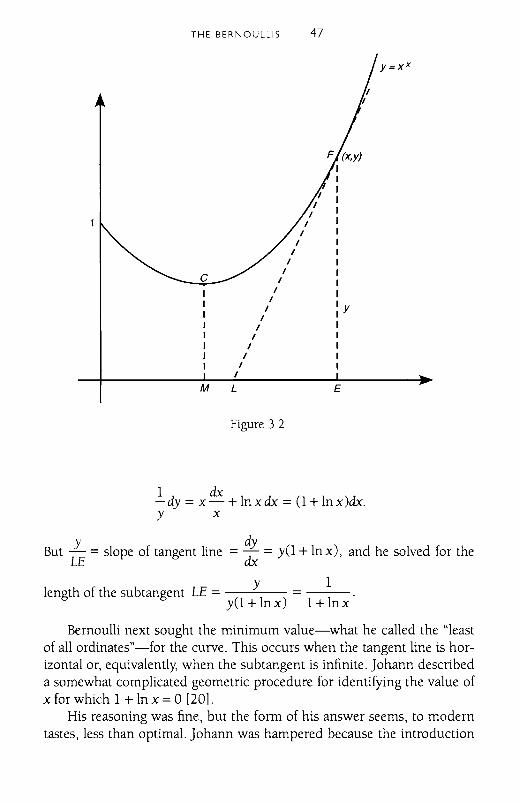
THE BERNOULLIS 47

~

//

//

//

//

//

// Y

//

//

//

/

M L E

Figure 3 2

1 dx-dy =x- + lnxdx = 0 + lnx)dx.y x

y ~But - = slope of tangent line = dx = yO + In x), and he solved for the

LE

length of the subtangent LE = ( YI) 1y 1+ nx 1+ lnx

Bernoulli next sought the minimum value-what he called the "leastof all ordinates"-for the curve. This occurs when the tangent line is hor­izontal or, equivalently, when the subtangent is infinite. Johann describeda somewhat complicated geometric procedure for identifying the value ofx for which 1 + In x =0 [20].

His reasoning was fine, but the form of his answer seems, to moderntastes, less than optimal. Johann was hampered because the introduction

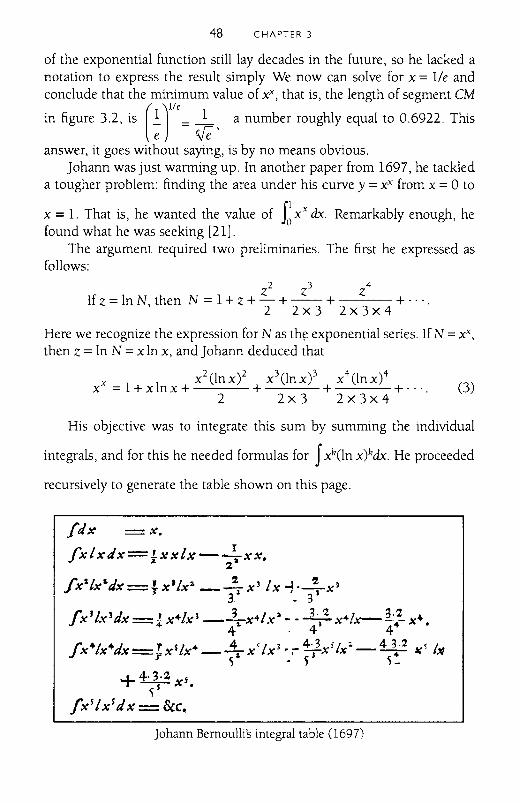
48 CHAPTER 3

of the exponential function still lay decades in the future, so he lacked anotation to express the result simply We now can solve for x = lie andconclude that thelm1i~}:num value of xx, that is, the length of segment eMin figure 3.2, is ~ = _1_, a number roughly equal to 0.6922. This

e ifCanswer, it goes without saying, is by no means obvious.

Johann was just warming up. In another paper from 1697, he tackleda tougher problem: finding the area under his curve y = XX from x = 0 to

p xx = 1. That is, he wanted the value of Jo x dx. Remarkably enough, hefound what he was seeking [21].

The argument required two preliminaries. The first he expressed asfollows:

Z2 Z3 Z4If z = In N, then N = 1+ z + - +-- + + ....

2 2x3 2x3x4

Here we recognize the expression for N as th~ exponential series. If N =xx,then Z = In N = x In x, and Johann deduced that

x 1 I x2(lnx)2 x\lnx)3 x4(lnx)4x = + x nx + + + +.... (3)

2 2x3 2x3x4

His objective was to integrate this sum by summing the individual

integrals, and for this he needed formulas for fxk(ln x)kdx. He proceeded

recursively to generate the table shown on this page.

fdx =."<.

fxlxdx=!xxlx-~xx•.& 2

fx''lxzdx=fxtlxa _"';"x3Ix-i'~x33 - 3

fx Jl<c 3dx=[ x4lx 3-+x~lx" - - 3.)'2 x41x-~i-x+.4 . 4 4

fx4Ix4dx=IxJlx4_~x'lxl .... \3x5Ix._4 ~.2 ~I I~so ~ • ) L

+ 4::l.:3 js x.)

fxslxsdx=&c.

Johann Bernoulli's integral table (1697)

THE BERNOULLIS 49

A modern approach would apply integration by parts to prove thereduction formula

For m =n = 1, the recursion in (4) gives

f 1 2 If 1 2 1 2xlnxdx ="2 x lnx -"2 xdx ="2 x lnx -"4 x .

(Like Bernoulli and other mathematicians of his day, we have ignoredU+ C' at the end of the integration formula.) For m = n = 2, we have

f 2 2 1 3 2 2f 2X (In x) dx = "3 x (In x) -"3 x (In x)dx

13 2 2[1 3 If 2 ]= - x (In x) - - - x In x - - x dx3 3 3 3

1 3 2 2 3 2 3= -x (lnx) - -x lnx +-x3 9 27'

where we have also applied (4) Wlth m = 2 and n = 1.In this fashion, we replicate Bernoulli's list of integrals. Along Wlth the

exponential series in (3), this was the key to solving his curious problem.

I xII 1 ~ (_I)k+ITheorem: r x dx = 1 - - + - - - + ... =~ ---

Jo 22 33 44 t kk

Proof: By (3), f;X'dx = f; [1 + x [n x + x2(l~ x)'

x 3(ln X)3 x4(ln X)4 ]dx+ + + ...

2x3 2x3x4

= Pdx + Px In xdx +~ Px 2(ln x)2dxJo Jo 2 Jo

+ _1_ Px\ln x)3dx2 X 3 Jo

1 11 4 4+ X (In x) dx + ... ,2x3x4°

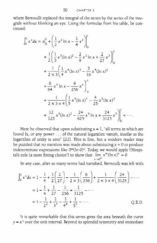
50 CHAPTER 3

where Bernoulli replaced the integral of the series by the series of the inte­grals without blinking an eye. Using the formulas from his table, he con­tinued:

s: x'dx =xl: + (~x'ln x- ~ x')[

( JI

11 3 2 2 3 2 3+ - - x (In x) - - x In x + - x2 3 9 27 0

1 (1 4 3 3 4 2+ -- - x (In x) - - x (In x)2 x 3 4 16

JI1

6 4 6 4+-x lnx--x64 256 0

1 (1 4+ - x 5(ln X)4 - - x 5(ln X)32 x 3 x 4 5 25

JI1

12 5 2 24 5 24 5+-x (lnx) --x lnx+--x + ....125 625 3125 0

Here he observed that upon substituting x = 1, "all terms in which arefound lx, or any power ... of the natural logarithm vanish, insofar as thelogarithm of unity is zero" [22]. This is fine, but a modern reader maybe puzzled that no mention was made about substituting x =0 to produceindeterminate expressions like Om(ln O)n. Today, we would apply l'Hospi­tal's rule (a most fitting choice!) to show that lim xm(In xt = a

X--7o+

In any case, after so many terms had vanished, Bernoulli was left with

It is quite remarkable that this senes gives the area beneath the curvey =XX over the unit interval. Beyond its splendid symmetry and immediate

THE BERNOULLIS 51

visual appeal, it has another attnbute not lost on Johann. He noted, "Thiswonderful series converges so rapidly that the tenth term contnbutes onlya thousandth of a millionth part of unity to the sum" [23]. To be sure, it

takes only a handful of terms to calculate J~ XXdx :::: 0.7834305107 accu­rately to ten places.

As the examples in this chapter should make clear, Jakob and JohannBernoulli were worthy disciples of Gottfried Wilhelm Leibniz. In theirhands, his calculus became, as we might say today, "user-friendly" Thebrothers left the subject in a more sophisticated yet much more under­standable state than they found it.

And Johann had one other legacy In the I 720s, he mentored a youngSWISS student of almost limitless promise. The student's name was Leon­hard Euler, and we sample his work next.

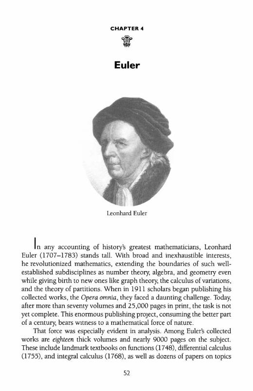
CHAPTER ..

Euler

Leonhard Euler

In any accounting of historys greatest mathematicians, LeonhardEuler (1707-1783) stands tall. With broad and inexhaustible interests,he revolutionized mathematics, extending the boundaries of such weU­established subdisciplines as number theory, algebra, and geometry evenwhile giving birth to new ones like graph theory, the calculus of variations,and the theory of partitions. When in 1911 scholars began publishing hiscollected works, the Opera omnia, they faced a daunting challenge. Today,after more than seventy volumes and 25,000 pages in print, the task is notyet complete. This enonnous publishing proJect, consuming the better partof a century, bears WltnesS to a mathematical force of nature.

That force was especially evident in analysis. Among Eulers collectedworks are eighteen thick volumes and nearly 9000 pages on the subject.These include landmark textbooks on functions (1748), differential calculus(1755), and integral calculus (1768), as well as dozens of papers on topics

52

EULER 53

ranging from differential equations to infinite series to elliptic integrals. As aconsequence, Euler has been descnbed as "analysis incarnate" [1].

It is impossible to do Justice to these contributions in a short chapter.Rather, we have selected five topics to illustrate the sweep of Euler'sachievements. We begin with an example from elementary calculus, fea­turing the bold-some may say reckless-approach so characteristic ofhis work.

A DIFFERENTIAL FROM EULER

In his text Institutiones calculi differentialis of 1755, Euler presented thefamiliar formulas of differential calculus [2]. These depended upon thenotion of "infinitely small quantities," which he characterized as follows:

There is no doubt that any quantity can be diminished until it allbut vanishes and then goes to nothing. But an infinitely smallquantity is nothing but a vanishing quantity, and so it is reallyequal to O.... There is really not such a great mystery lurking inthis idea as some commonly think and thus have rendered thecalculus of the infinitely small suspect to so many. [3]

For Euler, the differential dx was zero: nothing more, nothing less-inshort, nothing at all. The expressions x and x + dx were therefore equaland could be interchanged as the situation required. He observed that "theinfinitely small vanishes in comparison with the finite and hence can beneglected" [4]. Moreover, powers like (dx)2 or (dx)3 are infinitely smallerthan the infinitely small dx and likewise can be jettisoned at will.

It was often the ratio of differentials that Euler sought, and determiningthis ratio, which amounted to assigning a value to 0/0, was the mission ofcalculus. As he put it, "the whole force of differential calculus is concernedwith the investigation of the ratios of any two infinitely small quantities" [5].

As an illustration, we consider his treatment of the function y =sin x.Euler began with Newton's series (where we employ the modern "factori­al" notation):

. Z3 Z5 Z7sm Z = Z - - + - - - + . .. and

3! 5! 7!Z2 Z4 Z6

cos Z =1- - + - - - + ....2! 4! 6!

(1)

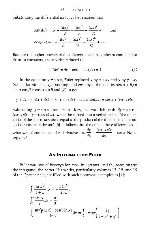
54 CHAPTER 4

Substituting the differential dx for z, he reasoned that

. (dx)3 (dx)5 (dxism(dx) = dx - --+-- - --+ ... and

3! 5! 7!

(dx)2 (dx)4 (dx)6cos(dx) = 1---+-----+ ....

2! 41 6!

Because the higher powers of the differential are insignificant compared todx or to constants, these series reduced to

sin(dx) = dx and cos(dx) = 1. (2)

In the equation y =sin x, Euler replaced x by x + dx and y by y + dy(which for him changed nothing) and employed the identity sin(a + {3) =sin a cos {3 + cos a sin {3 and (2) to get

y + dy =sin(x + dx) =sin x cos(dx) + cos x sin(dx) =sin x + (cos x)dx.

Subtracting y =sin x from both sides, he was left WIth dy =sin x +(cos x)dx - y =(cos x) dx, which he turned into a verbal recipe: "the differ­ential of the sine of any arc is equal to the product of the differential of the arcand the cosine of the arc" [6]. It follows that the ratio of these differentials-

dy (cosx)dxwhat we, of course, call the derivative-is dx = = cos x Noth-. ., dxmg to It.

AN INTEGRAL FROM EULER

Euler was one of history's foremost integrators, and the more bizarrethe integrand, the better. His works, particularly volumes 17, 18, and 19of the Opera omnia, are filled with such nontrivial examples as [7]:

rl (lnx)5 dx _ 31n6

Jo~ -- 252'

r=sinx dx =!!.-,Jo x 2

r1 sin(p In x) . cos(q In x) dx 1 (2P JJI = - arctan .o In x 2 1 _ p2 + q2

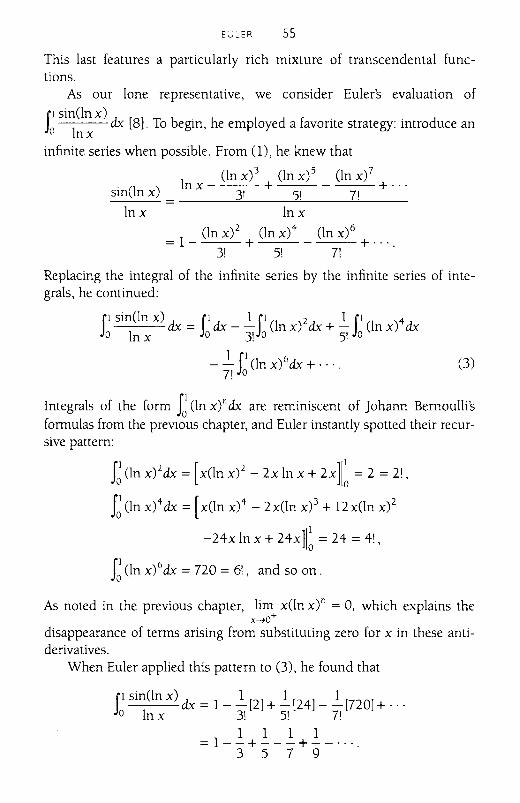
(3)

EULER 55

This last features a particularly rich mixture of transcendental func­tions.

As our lone representative, we consider Euler's evaluation off! sin(Inx)Jo I dx [8]. To begin, he employed a favorite strategy: introduce an

nxinfinite series when possible. From (1), he knew that

In x _ (In X)3 + (In X)5 _ (In x)7

+ ...sin(In x) = 31 5! 71

In x In x

= 1 _ (In X)2 + (In X)4 _ (In X)6 + ....3! 5! 7!

Replacing the integral of the infinite series by the infinite series of inte­grals, he continued:

p sin(In x) dx = P dx - ~ P (In x)2dx + ! P (In X)4 dxJo In x Jo 3!Jo 51 Jo

1 11 6- - (In x) dx + ....7! 0

Integrals of the form J~ (In x)ndx are reminiscent of Johann Bernoulli'sformulas from the preVlOUS chapter, and Euler instantly spotted their recur­sive pattern:

J~ (In x)2dx = [x(In X)2 - 2x In x + 2X][~ = 2 = 2!,

J~ (In X)4 dx = [x(In X)4 - 2x(In x)3 + 12x(In X)2

-24x In x + 24X][~ = 24 = 4!,

J~ (In x)6dx = 720 = 61, and so on.

As noted in the previous chapter, lim x(In x)n = 0, which explains thex~o+

disappearance of terms arising from substituting zero for x in these anti­derivatives.

When Euler applied this pattern to (3), he found that

11 sin(In x) 1 1 1---dx = 1- -[2]+ -[24]- -[720]+···

o In x 3! 5! 7!1 1 1 1=1--+---+-_···.3 5 7 9

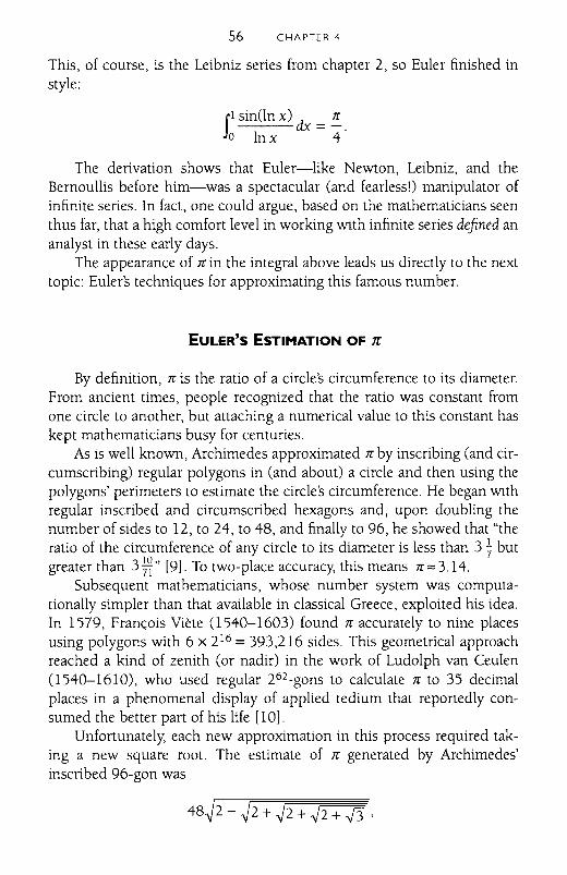
56 CHAPTER 4

This, of course, is the Leibniz series from chapter 2, so Euler finished instyle:

rsin(ln x) dx = !!....o lnx 4

The derivation shows that Euler-like Newton, Leibniz, and theBernoullis before him-was a spectacular (and fearless!) manipulator ofinfinite series. In fact, one could argue, based on the mathematicians seenthus far, that a high comfort level in working Wlth infinite series defined ananalyst in these early days.

The appearance of Jr in the integral above leads us directly to the nexttopic: Euler's techniques for approximating this famous number.

EULER'S ESTIMATION OF n

By definition, Jr is the ratio of a circles circumference to its diameter.From ancient times, people recognized that the ratio was constant fromone circle to another, but attaching a numerical value to this constant haskept mathematicians busy for centuries.

As is well known, Archimedes approximated Jr by inscribing (and cir­cumscribing) regular polygons in (and about) a circle and then using thepolygons' perimeters to estimate the circles circumference. He began Wlthregular inscribed and circumscribed hexagons and, upon doubling thenumber of sides to 12, to 24, to 48, and finally to 96, he showed that "theratio of the circumference of any circle to its diameter is less than 3 ~ butgreater than 3¥r" [9]. To two-place accuracy, this means Jr::::: 3.14.

Subsequent mathematicians, whose number system was computa­tionally simpler than that available in classical Greece, exploited his idea.In 1579, Franc;ois Viete (1540-1603) found Jr accurately to nine placesusing polygons with 6 x 216 =393,216 sides. This geometrical approachreached a kind of zenith (or nadir) in the work of Ludolph van Ceulen(1540-1610), who used regular 262_gons to calculate Jr to 35 decimalplaces in a phenomenal display of applied tedium that reportedly con­sumed the better part of his life [10].

Unfortunately, each new approximation in this process required tak­ing a new square root. The estimate of Jr generated by Archimedes'inscribed 96-gon was

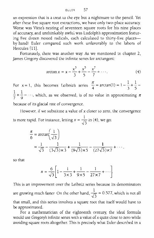
(4)

EULER 57

an expression that is a treat to the eye but a nightmare to the pencil. Yetafter these five square root extractions, we have only two-place accuracy.Worse was Viete's nesting of seventeen square roots for his nine placesof accuracy, and unthinkably awful was Ludolph's approximation featur­ing five dozen nested radicals, each calculated to thirty-five places­by hand! Euler compared such work unfavorably to the labors ofHercules [11].

Fortunately, there was another way. As we mentioned in chapter 2,James Gregory discovered the infinite senes for arctangent:

x 3 x 5 Xlarctan X = X - - + - - - + ....

3 5 7

nIlFor X = 1, this becomes Leibniz:S series - = arctan(l) = 1 - - + - ­

4351 1-:; +"9 - ..., which, as we observed, is of no value in approximating n

because of its glacial rate of convergence.

However, if we substitute a value of X closer to zero, the convergence

1is more rapid. For instance, letting x = -J3 in (4), we get

~ = arctan(~ )

1 1 1 1=-- + - + ...

-J3 (3-J3)x3 (9-J3) x 5 (27-J3)x7 '

so that

This is an improvement over the Leibniz series because its denominators

1are growing much faster On the other hand, -J3 "" 0.577, which is not all

that small, and this series involves a square root that itself would have tobe approximated.

For a mathematician of the eighteenth century, the ideal formulawould use Gregory:S infinite senes WIth a value ofx quite close to zero whileavoiding square roots altogether. This is precisely what Euler descnbed in a

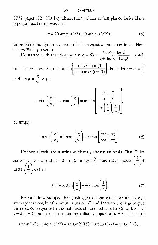
58 CHAPTER 4

1779 paper [12]. His key observation, which at first glance looks like atypographical error, was that

TC = 20 arctan(l/7) + 8 arctan(3/79). (5)

Improbable though it may seem, this is an equation, not an estimate. Hereis how Euler proved it. f3tan a - tan

He started with the identity tan(a - f3) = , which1+ (tan a)(tan f3)

[tana - tanf3 ] x

can be recast as a - f3 = arctan . Euler let tan a = -l+(tana)(tanf3) y

Zand tan f3 = - to get

W

x Z

arctan(~) - arctan( : ) = arctan _--=-y__w__

1+(~)(:) ,

or simply

arctan(~) = arctan(~) + arctan[XW - yz].y W yw+xz

(6)

He then substituted a string of cleverly chosen rationals. First, Euler

set x =y =Z =1 and w =2 in (6) to get ~ = arctan(l) = arctan(±) +

arctan(~), so that

TC = 4 arctan(±) + 4 arctan(~ ). (7)

He could have stopped there, using (7) to approximate TCvia Gregori,;arctangent series, but the input values of 1/2 and 1/3 were too large to givethe rapid convergence he desired. Instead, Euler returned to (6) with x = 1,Y =2, z = 1, and (for reasons not immediately apparent) w = 7. This led to

arctan(l/2) = arctan(l/7) + arctan(5115) = arctan(1I7) + arctan(l/3),

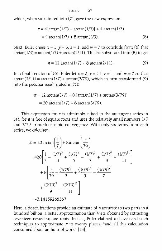
EULER 59

which, when substituted into (7), gave the new expression

7r= 4 [arctan(1/7) + arctan(l/3)] + 4 arctan(l/3)

=4 arctan(l17) + 8 arctan(1/3). (8)

Next, Euler chose x = 1, Y = 3, z = 1, and w = 7 to conclude from (6) thatarctan(l/3) =arctan(l17) + arctan(2/1l). This he substituted into (8) to get

7r =12 arctan(ll7) + 8 arctan(21l1). (9)

In a final iteration of (6), Euler let x = 2, Y = 11, z = 1, and w = 7 so thatarctan(2/11) = arctan(ll7) + arctan(3/79), which in turn transformed (9)into the peculiar result stated in (5):

7r= 12 arctan(ll7) + 8 [arctan(ll7) + arctan(3179)]

= 20 arctan(ll7) + 8 arctan(3179).

This expression for 7r is admirably suited to the arctangent series in(4), for it is free of square roots and uses the relatively small numbers 117and 3179 to produce rapid convergence. With only six terms from eachseries, we calculate

7r = 20 arctan(f)+ 8 arctan( :9)

='=20[~ _ (117)3 + (lI7)5 _ (lI7)7 + (lI7)9 _ (117)11]

7 3 5 7 9 11

+ 8[2_(3/79)3 + (3/79)5 (3179)7

79 3 5 7

+ (3/79)9 _ (3/79)11]

9 11

=,=3.14159265357.

Here, a dozen fractions provide an estimate of 7r accurate to two parts in ahundred billion, a better approximation than Viete obtained by extractingseventeen nested square roots. In fact, Euler claimed to have used suchtechniques to approximate 7r to twenty places, "and all this calculationconsumed about an hour of work" [13].

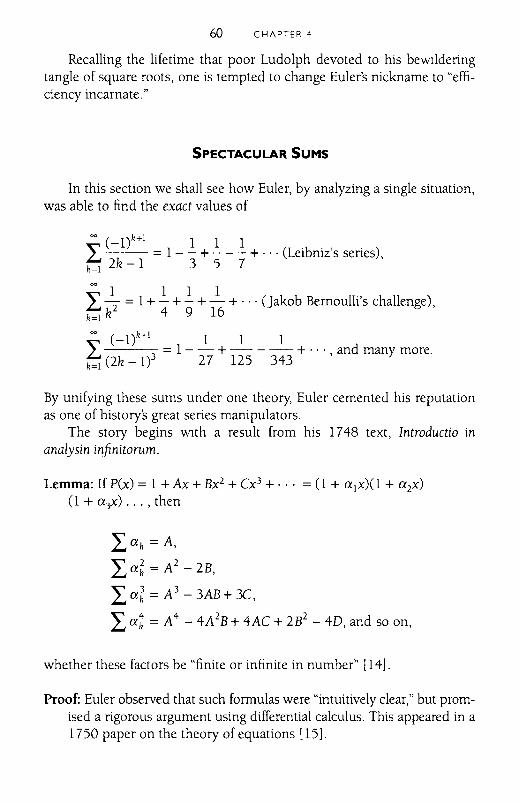
60 CHAPTER 4

Recalling the lifetime that poor Ludolph devoted to his beWIlderingtangle of square roots, one is tempted to change Euler's nickname to "effi­ciency incarnate."

SPECTACULAR SUMS

In this section we shall see how Euler, by analyzing a single situation,was able to find the exact values of

00 (_d+! 1 1 1 ..,.L =1- - + - - - + ... (Lelbmz s senes),k=! 2k -1 3 5 7

00 1 1 1 1 ,L 2 = 1+ - + - + - + ... (Jakob Bernoulli s challenge),k=! k 4 9 16

00 (_I)k+! 1 1 1L = 1 - - + - - -- + . .. and many more.k=l (2k _1)3 27 125 343 '

By unifying these sums under one theory, Euler cemented his reputationas one of historys great series manipulators.

The story begins WIth a result from his 1748 text, Introductio inanalysin infinitorum.

Lemma: If P(x) = 1 + Ax + Bx2 + Cx3 + ... = (l + a!x)(l + a2x)(l + a3x) ... , then

Lak = A,

La~ = A2

- 2B,

La~ = A3- 3AB+ 3C,

La: = A4- 4A2B+ 4AC + 2B2

- 4D, and so on,

whether these factors be "finite or infinite in number" [14].

Proof: Euler observed that such formulas were "intuitively clear," but prom­ised a rigorous argument using differential calculus. This appeared in a1750 paper on the theory of equations [15].

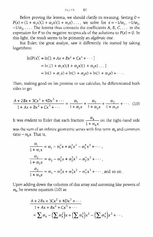
EULER 61

Before proving the lemma, we should clarify its meaning. Setting 0 =P(x)=(l+a1x)(l+a2x)(l+a3x) ... , we solve for x=-l/a1, -l/a2,-l!a3 , .•.. The lemma thus connects the coefficients A, B, C, ... in theexpression for P to the negative reciprocals of the solutions to P(x) = O. Inthis light, the result seems to be primanly an algebraic one.

But Euler, the great analyst, saw it differently. He started by takinglogarithms:

In[P(x)] =In[1 + Ax + Bx2 + Cx3 + ... ]

=In[(l + a1x)(l + a2x)(l + a 3x) ... ]

= In(1 + a1x) + In(l + a2x) + In(l + a3x) + ....

Then, making good on his promise to use calculus, he differentiated bothsides to get

A + 2Bx + 3Cx 2 + 4Dx3 + .

1+ Ax + Bx2 + Cx 3 + .(l0)

It was evident to Euler that each fraction a k on the right-hand side1+ akx

was the sum of an infinite geometric senes Wlth first term ak and commonratio - akx. That is,

a 1 2 3 2 4 3----'-- = a 1 - a 1x + a 1x - a 1x + ...1+ a\x

a2 2 3 2 4 3---=---- = a 2 - a2x + a 2x - a2 x + ...1+ a2x

a 3 2 3 2 4 3 d=a 3 - a 3x + a 3 x - a3x + ... , an so on.1+ a 3x

Upon adding down the columns of this array and summing like powers ofak , he rewrote equation (l0) as

A + 2Bx + 3Cx2 + 4Dx 3 + .

1+ Ax + Bx2 + Cx 3 + .

=Lak -(La~)x+(La~)x2 -(La~)x3+ ....

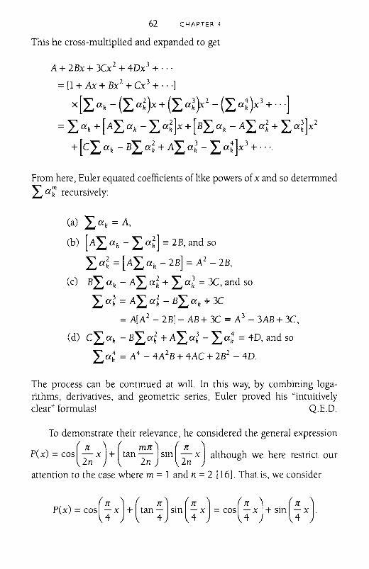
62 CHAPTER 4

This he cross-multiplied and expanded to get

A + 2Bx + 3Cx2+ 40x 3 + ' , ,

= [1 + Ax + Bx2 + CX 3 + ' , ,]

X[L a h - (L aOx + (L a~~2 - (L anX3 +, ..]

=Lah + [ALah - La~]x + [BLah - ALa~ + La~]x2

+ [CLah - BLa~ + ALa~ - L anx3 + .. '.

From here, Euler equated coefficients of like powers of x and so determined

L a~ recursively:

(a) Lah = A,

(b) [ALah - La~] = 2B, and so

La~ = [ALah - 2B] = A2

- 2B,

(c) BLah - ALa~ + La~ = 3C, and so

La~ = ALa~ - BLah + 3C

=A[A2 - 2B] - AB+ 3C = A3- 3AB+ 3C,

(d) CLah - BLa; +ALa~ - La: = 40, and so

La: = A4- 4A2B+ 4AC + 2B2 - 40.

The process can be continued at WIll. In this way, by combining loga­rithms, derivatives, and geometric series, Euler proved his "intuitivelyclear" formulas! Q.E.D.

To demonstrate their relevance, he considered the general expression

p(x) = cos (:n x ) + (tan ~: ) sin (:n x) although we here restrict our

attention to the case where m = 1 and n = 2 [16]. That is, we consider

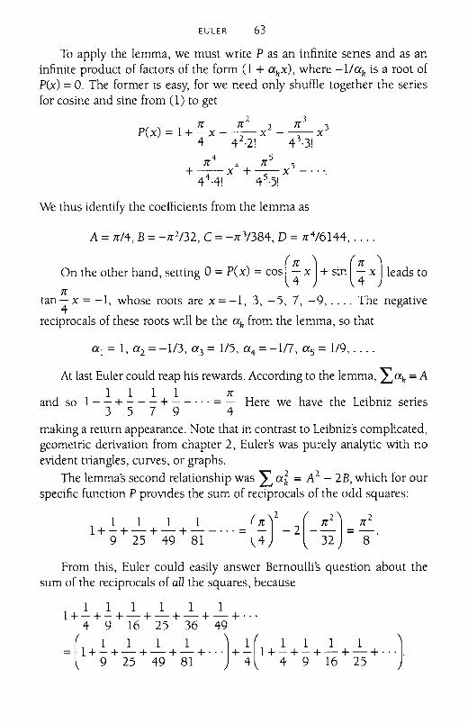
EULER 63

To apply the lemma, we must write P as an infinite senes and as aninfinite product of factors of the form (1 + akx), where -l/ak is a root ofP(x) =O. The former is easy, for we need only shuffle together the seriesfor cosine and sine from (1) to get

;r ;r2 2 ;r3 3P(x) = 1+ - x - -- x - -- x

4 4 2·2! 4 3'31;r4 4 ;r5 5

+--x +--x44·4! 4 5·s!

We thus identify the coefficients from the lemma as

A = ;r/4, B = -;r2/32, C = -;r3/384, D = ;r4/6144, ....

On the other hand, setting 0 = P(x) = cos ( ~ x ) + sin (~ x ) leads to;r

tan - x = -1, whose roots are x = -1, 3, -5, 7, -9, .... The negative4

reciprocals of these roots WIll be the ak from the lemma, so that

a j = 1, a2 = -1/3, a3 = liS, a4 = -1/7, as = 1/9, ....

At last Euler could reap his rewards. According to the lemma, LPk =A1 1 1 1 ;r

and so 1 - - + - - - + - - ... = - Here we have the Leibniz series3 5 7 9 4

making a return appearance. Note that in contrast to Leibniz's complicated,geometric derivation from chapter 2, Euler's was purely analytic with noevident triangles, curves, or graphs.

The lemma's second relationship was L a~ = A2- 2B, which for our

specific function P proVIdes the sum of reciprocals of the odd squares:

1+i+ 215+ ;9 + ;1 -. =(~r-+;~)<From this, Euler could easily answer Bernoulli's question about the

sum of the reciprocals of all the squares, because

1 1 1 1 1 11+-+-+-+-+-+-+···

4 9 16 25 36 49

= (1 +~ + J.- + _1_ + J.- + ...J+ ~(1 +~ + ~ + J.- + _1 + ...J.9 25 49 81 4 4 9 16 2S

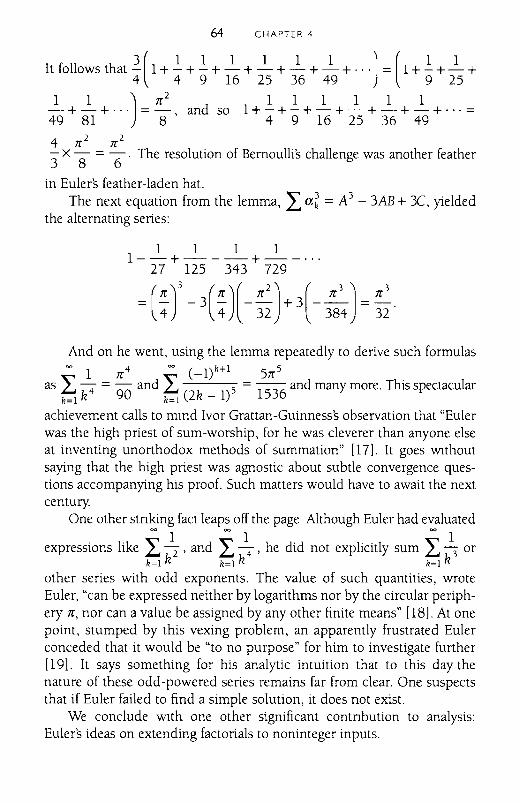
64 CHAPTER 4

3( 1 1 1 1 1 1 ) ( 1 1It follows that - 1+ - + - + - + - + - + - + -_. = 1+ - + - +4 4 9 16 25 36 49 9 25

~ +~ + ...) = 1(2 and so 1+ ..!. + ..!. +~ +~ +~ + _1 + ... =49 81 8 ' 4 9 16 25 36 494 1(2 1(2

3" X 8 =6· The resolution of Bernoullis challenge was another feather

in Euler's feather-laden hat.The next equation from the lemma, L a~ = A3

- 3AB + 3C, yieldedthe alternating series:

1 1 1 11--+---+----­

27 125 343 729

And on he went, using the lemma repeatedly to derive such formulas= 1 1(4 = (_I)k+1 51(5

as L 4" = - and L 5 = 1 36 and many more. This spectaculark=l k 90 k=l (2k - 1) 5

achievement calls to mind Ivor Grattan-Guinness's observation that "Eulerwas the high priest of sum-worship, for he was cleverer than anyone elseat inventing unorthodox methods of summation" [171. It goes WIthoutsaying that the high priest was agnostic about subtle convergence ques­tions accompanying his proof. Such matters would have to await the nextcentury.

One other stnking fact leaps off the page Although Euler had evaluated= 1 = 1 = 1

expressions like L 2:" ' and L 4"' he did not explicitly sum L 3 ork=l k k=l k k=l k

other series with odd exponents. The value of such quantities, wroteEuler, "can be expressed neither by logarithms nor by the circular periph­ery 1(, nor can a value be assigned by any other finite means" [18]. At onepoint, stumped by this vexing problem, an apparently frustrated Eulerconceded that it would be "to no purpose" for him to investigate further[191. It says something for his analytic intuition that to this day thenature of these odd-powered series remains far from clear. One suspectsthat if Euler failed to find a simple solution, it does not exist.

We conclude WIth one other significant contnbution to analysis:Euler's ideas on extending factorials to noninteger inputs.

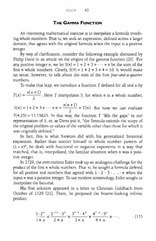
EULER 65

THE GAMMA FUNCTION

An interesting mathematical exercise is to interpolate a formula involv­ing whole numbers. That is, we seek an expression, defined across a largerdomain, that agrees with the original formula when the input is a positiveinteger.

By way of clarification, consider the folloWIng example discussed byPhilip Davis in an article on the origins of the gamma function [20]. Forany positive integer n, we let Sen) = 1 + 2 + 3 + ... + n be the sum of thefirst n whole numbers. Clearly, 5(4) = 1 + 2 + 3 + 4 = 10. It would makeno sense, however, to talk about the sum of the first four-and-a-quarternumbers.

To make that leap, we introduce a function T defined for all real x by

x(x + 1)T(x) = 2 . Here T interpolates 5, for when n is a whole number,

n(n + 1)Sen) = 1+ 2 + 3 + ... + n = = TCn). But now we can evaluate

2T(4.25) = 11.15625. In this way, the function T "fills the gaps" in ourrepresentation of 5, or, as DaVIs put it, "the formula extends the scope ofthe original problem to values of the variable other than those for which itwas originally defined."

In fact, this is what Newton did with his generalized binomialexpansion. Rather than restrict himself to whole number powers ofo + x)n, he dealt with fractional or negative exponents in a way thatmatched, that is, interpolated, the familiar situation when n was a posi­tive integer.

In 1729, the ever-curious Euler took up an analogous challenge for theproduct of the first n whole numbers. That is, he sought a formula definedfor all positive real numbers that agreed WIth 1 . 2 . 3 ..... n when theinput n was a positive integer. To use modern terminology, Euler sought tointerpolate the factorial.

His first solution appeared in a letter to Chnstian Goldbach fromOctober of 1729 [21]. There, he proposed the bizarre-looking infiniteproduct

1.2 X 21- x .y 31- x .4 x 4 1- x ·5x

--x x X x··· (1)l+x 2+x 3+x 4+x

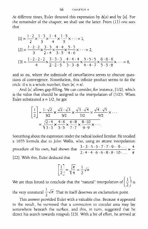
66 CHAPTER 4

At different times, Euler denoted this expression by ~(x) and by [x]. Forthe remainder of the chapter, we shall use the latter. From (11) one seesthat

1·2 1·3 1·4 1·5[l]=-x-x-x-x···=l

2 345 '1·2·2 3·3 4·4 5·5

[2] = x--x--x--x··· = 2,3 2·4 3·5 4·6

1·2·2·2 3·3·3 4·4·4 5·5·5 6·6·6[3] = x x x x x ... = 6,

4 2·2·5 3·3·6 4·4·7 5·5·8

and so on, where the infinitude of cancellations serves to obscure ques­tions of convergence. Nonetheless, this infinite product seems to do thetrick: if n is a whole number, then [n] =n!.

And [x] allows gap-filling. We can consider, for instance, [1/2], whichis the value that should be assigned to the interpolation of 0/2)!. WhenEuler substituted x = 1/2, he got

[~] = 1·.fi x .fi . -J3 x -J3 .-f4 x -f4 .-J5 x ...2 3/2 5/2 7/2 9/2

= ~2' 4 x 4·6 x 6·8 x 8 ·10 x . ".3·3 5·5 7·7 9·9

Something about the expression under the radical looked familiar. He recalleda 1655 formula due to John Wallis, who, using an arcane interpolattion

3·3· 5·5· 7·7·9· 9·... 4procedure of his own, had shown that =

2·4·4·6·6·8·8·10· ... Jr

[22]. With this, Euler deduced that

[l]=~ =l~·We are thus forced to conclude that the "natural" interpolation of (±}is

1the very unnatural '2~' That in itself deserves an exclamation point.

This answer provided Euler with a valuable clue. Because Jr appearedin the result, he surmised that a connection to circular area may laysomewhere beneath the surface, and this, in turn, suggested that hedirect his search towards integrals [23]. With a bit of effort, he arrived at

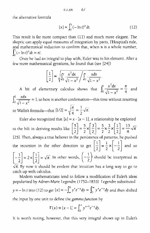
EULER 67

the alternative formula

[x] = S;(-lntYdt. (12)

This result is far more compact than (11) and much more elegant. Theskeptic can apply equal measures of integration by parts, I'Hospital's rule,and mathematical induction to confirm that, when n is a whole number,

S; (- In ttdt = n!.

Once he had an integral to play with, Euler was in his element. After afew more mathematical gyrations, he found that (see [24])

f! x2dx If! xdx

JO~I_x2 Jo~'

11 x2dx 7r

A bit of elementary calculus shows that ~ = - and0...;1- x- 4

rl xdxJI ~ = 1, so here is another confirmation-this time without resorting0...;1- x-

to Wallis's formula-that [112] = ~ = ~-Jn.f4 2Euler also recognized that [x] =x . [x - 1], a relationship he exploited

to the hilt in deriving results like [~] = ~ x [~] = ~ x ~ x [~] = ~-J1i2222228

[25]. Then, always a true believer in the persistence of patterns, he pushed

the recursion in the other direction to get [1] =1x [-1] and so

[-1] = 2 x [1] = -In. In other words, (-1} should be interpreted as

.JJi. By now it should be eVIdent that intuition has a long way to go tocatch up With calculus.

Modern mathematicians tend to follow a modification of Eulers ideaspopularized by Adnen-Marie Legendre (1752-1833). Legendre substituted

y = -In t into (12) to get [x] = - S~yXe-Ydy = S; yXe-Ydy and then shifted

the input by one unit to define the gamma function by

rex) == [x -1] = S; yX-Ie-Ydy.

It is worth noting, however, that this very integral shows up in Euler's

68 CHAPTER 4

writings as well [26].Of course, the gamma function inherits properties that Euler had dis­

covered about [x], such as the recursion rex + 1) =xrex) or the remarkableidentity f(l/2) = [-112] =.fii. It is a function that seems to appear any­where sophisticated mathematical analysis is practiced, from probabilityto differential equations to analytic number theory. Nowadays, the gammafunction is regarded as the first and perhaps most important of the "high­er functions" of analysis, that is, those whose very definition requires theideas of calculus. It occupies a place beyond the algebraic, exponential, ortrigonometnc functions that characterize elementary mathematics. Andwe owe it, like so much else, to Euler.

The results of this chapter-be they differentials or integrals, approxi­mations or interpolations-reveal an astonishing ingenuity. Von Neumanncalled Euler "the greatest virtuoso of the period," for he posed the rightquestions and, WIth an agility and intuition that continue to amaze, regu­larly found the right answers [27]. Without doubt, Euler was at home inanalysis, the perfect arena in which to apply what seemed to be his infor­mal credo: Follow the formulas, and they will lead to the truth

No one ever did it better.

CHAPTER 5

First Interlude

Leonhard Euler died in 1783, one year short of the centennial ofLeibniz's first paper on differential calculus. By any measure, it had been aremarkable century in the history of mathematics. The results consideredthus far, although a tiny fraction of the centurys output, illustrate theprogress that had been made. Grappling with infinite processes to discovercorrect and sometimes spectacular results, Newton, Leibniz, the Bernoullis,and Euler had established calculus as the mathematical subdiscipline parexcellence. Our hats are off to these great originators.

An important trend of that first century was a shift in perspective fromthe geometric to the analytic. As the problems became more challenging,their solutions depended less on the geometry of curves than on the alge­bra of functions. The complicated diagrams that Leibniz used to prove histransmutation theorem in 1673 had no counterpart in Euler's work fromthe middle of the eighteenth century. In this sense, analysis had assumed amore modern look.

But other familiar aspects of the subject were nowhere to be seen.Largely missing, for instance, was that bulwark of modern analysis, theinequality. Seventeenth and eighteenth century mathematicians dealtmainly in equations. Their work tended to employ clever substitutions thattransformed one formula into another so as to emerge with the desiredanswer. Although Jakob Bernoullis divergence proof of the harmonicsenes (see chapter 3) featured a deft use of inequalities, such an approachwas rare.

Rare as well was the study of broad classes of functions. Euler and hispredecessors were adept at looking at specific integrals or series, but theywere less interested in common properties of, say, continuous or differen­tiable functions. A shift in focus from the specific to the general would bea hallmark of the coming century.

One other striking difference between early calculus and that of todayis the attention given to logical foundations. As we have seen, mathemati­cians of the period used results whose validity they had neither proved nor,

69

70 CHAPTER 5

in many cases, even considered. An example was the tendency to replacethe integral of an infinite series by the infinite series of integrals, that is, to

equate f:[~J.(X)}x and ~[f:J.(xldxI Both opecations here-

integrating functions and summing series-involve infinite processeswhose uncntical interchange can lead to incorrect results. Certain condi­tions must be met before a reversal of this sort is appropriate. On thisfront, the calculus pioneers operated more on intuition than on reason.Admittedly, their intuition was often very good, Wlth Euler in particularpossessing an uncanny ability to know Just how far he could go beforeplunging into the mathematical abyss.

Still, the foundations of calculus were suspect. As an illustration, werecall the role played by infinitely small quantities. Attempts to explainthese so-called infinitesimals-and everyone from Leibniz to Euler gave ita shot-never proved satisfactory. Like a mathematical chameleon, infini­tesimals seemed inevitably to be both zero and nonzero at the same time.At rock bottom, they were paradoxical, counterintuitive entities.

Nor were things much better when mathematicians based their con­clusions on "vanishing" quantities. Newton was a proponent of thisdynamic approach, a fitting position, perhaps, for one so captivated by thestudy of motion. Introducing what we now call the derivative, he consid­ered a quotient of vanishing quantities and wrote that, by the "ultimateratio" of these evanescent quantities, he meant "the ratio of the quantitiesnot before they vanish, nor afterwards, but with which they vanish" [1].Besides conjuring up the notion of a quantity after it vanishes (whateverthat means), Newton asked his readers to imagine a ratio at the preciseinstant when-poon-both numerator and denominator simultaneouslydissolve into thin air. His description seemed ripe for criticism.

It was not long in coming, and the critic was George Berkeley(1685-1753), noted philosopher and Bishop of eloyne. In his 1734 essayThe Analyst, Berkeley ridiculed those scientists who accused him of pro­ceeding on faith and not reason, yet who themselves talked of infinitelysmall or vanishing quantities. To Berkeley this was at best fuzzy thinkingand at worst hypocrisy. The latter was implied in the long subtitle.

A Discourse Addressed to an Infidel Mathematician, wherein It IsExamined Whether the Object, Principles, and Inferences of theModern Analysis Are More Distinctly Conceived, or More Evi­dently Deduced, than Religious Mysteries and Points of Faith [2]

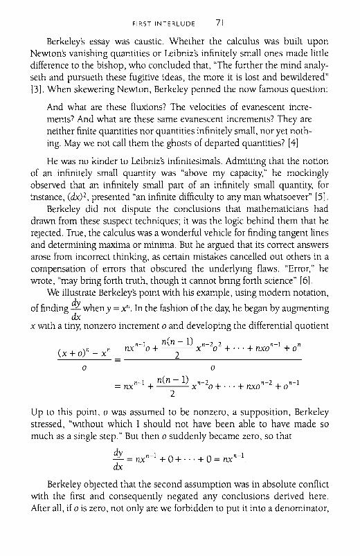
FIRST INTERLUDE 71

Berkeley's essay was caustic. Whether the calculus was built uponNewtons vanishing quantities or Leibniz's infinitely small ones made littledifference to the bishop, who concluded that, 'The further the mind analy­seth and pursueth these fugitive ideas, the more it is lost and bewildered"13]. When skewering Newton, Berkeley penned the now famous question:

And what are these fluxions? The velocities of evanescent incre­ments? And what are these same evanescent increments? They areneither finite quantities nor quantities infinitely small, nor yet noth­ing. May we not call them the ghosts of departed quantities? [4]

He was no kinder to Leibniz's infinitesimals. Admitting that the notionof an infinitely small quantity was "above my capacity," he mockinglyobserved that an infinitely small part of an infinitely small quantity, forinstance, (dx)2, presented "an infinite difficulty to any man whatsoever" [5].

Berkeley did not dispute the conclusions that mathematicians haddrawn from these suspect techniques; it was the logic behind them that herejected. True, the calculus was a wonderful vehicle for finding tangent linesand determining maxima or minima. But he argued that its correct answersarose from incorrect thinking, as certain mistakes cancelled out others in acompensation of errors that obscured the underlyJ.ng flaws. "Error," hewrote, "may bring forth truth, though it cannot bnng forth science" [6].

We illustrate Berkeley's point with his example, using modem notation,

of finding dy when y =xn. In the fashion of the day, he began by augmentingdx

x Wlth a tiny, nonzero increment 0 and developing the differential quotient

n-l n(n - 1) n-2 2 n-l n(x + O)n _ X n nx 0 + 2 x 0 + ... + nxo + 0

-----=-------==------------o 0

n-l n(n- 1) n-2 n-2 n-l=nx + x o+···+nxo +0

2

Up to this point, 0 was assumed to be nonzero, a supposition, Berkeleystressed, "Wlthout which I should not have been able to have made somuch as a single step." But then 0 suddenly became zero, so that

dy n-l 0 0 n-l-=nx + + ... + =nx .dx

Berkeley objected that the second assumption was in absolute conflictwith the first and consequently negated any conclusions derived here.After all, if 0 is zero, not only are we forbidden to put it into a denominator,

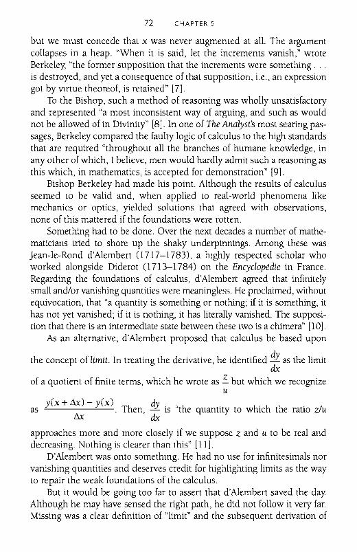
72 CHAPTER 5

but we must concede that x was never augmented at all. The argumentcollapses in a heap. "When it is said, let the increments vanish," wroteBerkeley, "the former supposition that the increments were something ...is destroyed, and yet a consequence of that supposition, Le., an expressiongot by VIrtue theoreof, is retained" [7).

To the Bishop, such a method of reasoning was wholly unsatisfactoryand represented "a most inconsistent way of arguing, and such as wouldnot be allowed of in Divinity" [8). In one of The Analysts most searing pas­sages, Berkeley compared the faulty logic of calculus to the high standardsthat are required "throughout all the branches of humane knowledge, inany other of which, I believe, men would hardly admit such a reasoning asthis which, in mathematics, is accepted for demonstration" [9J.

Bishop Berkeley had made his point. Although the results of calculusseemed to be valid and, when applied to real-world phenomena likemechanics or optics, yielded solutions that agreed with observations,none of this mattered if the foundations were rotten.

Something had to be done. Over the next decades a number of mathe­maticians tried to shore up the shaky underpinnings. Among these wasJean-Ie-Rond d'Alembert (1717-1783), a highly respected scholar whoworked alongside Diderot (1713-1784) on the Encyclopedie in France.Regarding the foundations of calculus, d'Alembert agreed that infinitelysmall and/or vanishing quantities were meaningless. He proclaimed, withoutequivocation, that "a quantity is something or nothing; if it is something, ithas not yet vanished; if it is nothing, it has literally vanished. The supposi­tion that there is an intermediate state between these two is a chimera" [10).

As an alternative, d'Alembert proposed that calculus be based upon

the concept of limit. In treating the derivative, he identified dy as the limitdx

of a quotient of finite terms, which he wrote as ~ but which we recognizeu

y(x +~) - y(x) Th dy." h . h' h h . z/as . en, - IS t e quantIty to w lC t e ratIO U~ dx

approaches more and more closely if we suppose Z and U to be real anddecreasing. Nothing is clearer than this" [II).

D'Alembert was onto something. He had no use for infinitesimals norvanishing quantities and deserves credit for highlighting limits as the wayto repair the weak foundations of the calculus.

But it would be going too far to assert that d'Alembert saved the dayAlthough he may have sensed the right path, he did not follow it very far.Missing was a clear definition of "limit" and the subsequent derivation of

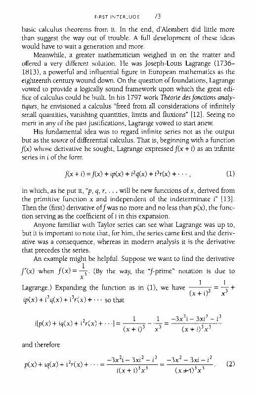
FIRST INTERLUDE 73

basic calculus theorems from it. In the end, d'Alembert did little morethan suggest the way out of trouble. A full development of these ideaswould have to wait a generation and more.

Meanwhile, a greater mathematician weighed in on the matter andoffered a very different solution. He was Joseph-Louis Lagrange 0736­1813), a powerful and influential figure in European mathematics as theeighteenth century wound down. On the question of foundations, Lagrangevowed to provide a logically sound framework upon which the great edi­fice of calculus could be built. In his 1797 work Theone des jonctions analy­

tiques, he envisioned a calculus "freed from all considerations of infinitelysmall quantities, vanishing quantities, limits and fluxions" [12]. Seeing nomerit in any of the past justifications, Lagrange vowed to start anew.

His fundamental idea was to regard infinite series not as the outputbut as the source of differential calculus. That is, beginning with a functionj(x) whose derivative he sought, Lagrange expressed j(x + i) as an infiniteseries in i of the form

j(x + i) = j(x) + ip(x) + i2q(x) + i3r(x) + ... , 0)

in which, as he put it, "p, q, r, ... will be new functions of x, derived fromthe primitive function x and independent of the indeterminate i" [13].Then the (first) derivative ofj was no more and no less than p(x), the func­tion serving as the coefficient of i in this expansion.

Anyone familiar Wlth Taylor series can see what Lagrange was up to,but it is important to note that, for him, the series came first and the deriv­ative was a consequence, whereas in modern analysis it is the derivativethat precedes the series.

An example might be helpful. Suppose we want to find the derivative1

rex) when j(x) =3' (By the way, the 'J-prime" notation is due tox

1 1Lagrange.) Expanding the function as in 0), we have --- =- +

(x+ d x3

ip(x) + i 2q(x) + i\(x) + ... so that

1 1ilp(x) + iq(x) + i 2r(x) + ...J = 3

(x + i) x 3

and therefore

-3x 2i - 3xi 2- i 3

(x + i)3 x 3

3 2· 3. 2 . 3 2 3 22 - X 1- Xl - I -3x - xi - ip(x) + iq(x) + i rex) + ... = 3 3 = ---.,-----,-

i(x + i) x (x =1-0"'0 3x 3(2)

74 CHAPTER 5

-3x2 -3At this point, Lagrange let i =0 in (2) to get p(x) = -6-' Thus, j'(x) = 4""'

x xwhich of course would have been no surprise to Newton or Leibniz.

For Lagrange, this derivation avoided quantities that were infinitelysmall as well as those ghosts of departed quantities vanishing into obliVIon.LikeW1se, he had no need for d'Alemberts uncertainly defined limits. WhenLagrange let i =0, he meant that literally. No pitfalls were encountered in(2), for no zero appeared in any denominator. He regarded this as a purelyanalytic approach to the derivative, one requiring none of the logical gyra­tions that had embarrassed his predecessors. It was all so neat and tidy

Or was it? For one thing, defining derivatives in this manner is terri­bly indirect. The ideas of Newton and Leibniz-even if cluttered withcurves and triangles and resting upon a shaky foundation-were at leaststraightforward in their object. Lagrange's ideas, presented without a sin­gle diagram, completely obscured the fact that derivatives had somethingto do with slopes of tangent lines.

That is a minor cnticism. More troubling was the question of how toproceed for less triVIal functions than that given above. In our example, the

1 1key was to expand and simplify 3 - 3 in order to factor i from the

(x + i) x

result. But where is the guarantee that every function could be so expandedand simplified? Where is the guarantee that a series so constructed is con­vergent? And where is the guarantee that a convergent series so construct­ed actually converges to the function we started with? These are deep andimportant questions.

Ultimately, the theory of Lagrange could not withstand this kind ofscrutiny. In 1822 the French mathematician Augustin-Louis Cauchy pub­lished an example that proved fatal to Lagrange's ideas. Cauchy, who willbe the subject of our next chapter, showed that the function

{

-lIx2

f(x) = e 0 if x :;:. 0,if x =0,

and all of its derivatives are zero at x =0 [14]. Consequently, as a powersenes about the origin, f(x) =0 + 0 . x + 0 . x2 + 0 . x3 + ... =0, which intum means that, if we begin W1thf and write it as a series, we end up with adifferent function than we started with! As a series, we would find it impos­sible to distinguish between f above and the constant function g(x) = o.

FIRST INTERLUDE 75

Cauchy's example of two distinct functions shanng a power series indicat­ed that analysis was considerably less benign than Lagrange had assumed.

In the end, a series-based definition of the derivative-and hence aseries-based foundation for the calculus-was abandoned. But if Lagrangefailed in his primary mission, he made a number of contributions thatanticipated the coming century. First, he elevated foundational questionsinto greater prominence, treating them as both interesting and importantissues. Second, he tried to derive the theorems of the calculus from hisbasic definitions, in the process introducing inequalities and exhibitingskill in their use. Finally, as Judith Grabiner observed in her book, TheOrigins of Cauchy's Rigorous Calculus:

On reading Lagrange's work, one is struck by his feeling for thegeneral. ... His extreme love of generality was unusual for thistime and contrasts WIth the emphasis of many of his contempo­raries on solving specific problems. His algebraic foundation forthe calculus was consistent WIth his generalizing tendency. [15]

All these contnbutions notwithstanding, the eighteenth century endedwith the logical crisis still unresolved. The work of d'Alembert andLagrange, along with others who addressed these matters, failed to mollifythe critics. As late as 1800, the words of Bishop Berkeley carried the ring oftruth: "I say that in every other Science Men prove their Conclusions by theirPrinciples, and not their Principles by the Conclusions" [16].

But a resolution was near. The same Cauchy who recognized thenonuniqueness of series would, in the early nineteenth century, see a wayto explain the foundations of calculus in a satisfactory manner. By the timehe was done, analysis would be a far more general, abstract, and inequality­laden subject than his predecessors could have imagined. And it would befar more rigorous.

It is to this towering figure, and to his revolution, that we now turn.

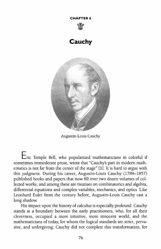
CHAPTER 6

Cauchy

Augustin-louis Cauchy

EriC Temple Bell, who popularized mathematicians in colorful ifsometimes immoderate prose, wrote that ~Cauchys pan in modem math­ematics is not far from the center of the stage" [11. It is hard to argue withthis Judgment. During his career, Augustin-Louis Cauchy (1789-1857)published books and papers that now fill over two dozen volumes of col·lected works, and among these are treatises on combinatorics and algebra,differential equatiOns and complex variables, mechanics, and optics LikeLeonhard Euler from the century before, Augustin-Louis Cauchy cast along shadow.

His impact upon the history of calculus is especially profound. Cauchystands at a boundary between the early practitioners, who, for all theircleverness, occupied a more intuitive, more innocent world, and themathematicians of today, for whom the logical standards are strict, perva­sive, and unforgivmg. Cauchy did not complete this transformation, for

76

CAUCHY 77

his ideas would require considerable fine tuning in the decades to come.But the similarity between Cauchy's development of analysis and that oftoday's textbooks cannot fail to impress the modern reader.

This chapter gives a taste of Cauchy in action. We include a number ofexamples, ranging from his theory of limits to the mean value theoremand from his definition of the integral to the fundamental theorem of cal­culus, before concluding with a pair of tests for series convergence. Thismaterial comes from two great texts: his 1821 Cours d'analyse de l'EcoleRoyale Polytechnique and his 1823 Resume des le~ons donnees a l'Ecole RoyalePolytechnique, sur Ie calcul infinitesimal [2].

LIMITS, CONTINUITY, AND DERIVATIVES

Although Cauchy recognized Lagrange as an elder statesman of math­ematics, he could not endorse the latters series-based definition of thederivative. "I reject the development of functions by infinite series," wroteCauchy, who continued:

I do not ignore that the illustrious [Lagrange] has taken this for­mula as the basis for his theory of derived functions. But, in spiteof the respect commanded by so great an authority, most geome­ters now acknowledge the uncertainty of results to which one canbe led by use of divergent series ... and we add that [Lagrange'smethods] lead to the development of a function by a convergentseries, although the sum of this series differs essentially from thefunction proposed. [3]

The last allusion is to Cauchy'S counterexample mentioned in the pre­vious chapter. For him, Lagranges program was a dead end. Hoping to

provide a logically valid alternative, Cauchy asserted that "the prinCiplesof differential calculus, and their most important applications, can easilybe developed without the need of senes."

Instead, Cauchy believed that the foundation upon which all calculuswould be built was the idea of limit. His definition of this concept is amathematical classic:

When the values successively attributed to a variable approachindefinitely to a fixed value, in a manner so as to end by differingfrom it by as little as one Wlshes, this last is called the limit of allthe others. [4]

78 CHAPTER 6

Cauchy gave the example of a circle's area as the limit of the areas ofinscribed regular polygons as the number of sides increases withoutbound. Of course, no polygonal area ever equals that of the circle. But forany proposed tolerance, an inscribed regular polygon can be found whosearea, and those of all inscribed regular polygons with even more sides, iscloser to that of the circle than the tolerance stipulated. Polygonal areasget close-and stay close-to the area of the circle. This is the essence ofCauchy's idea.

A modern reader may be surprised by his definition's wordiness, itsdynamiC imagery, and the absence of E and 8. Nowadays we do not talkabout a "succession" of numbers "approaching" something, and we tendto prefer the symbolic efficiency of "E > 0" to the phrase "as little as onewishes."

Yet this was an advance of the first order. Cauchys idea, based on"closeness," avoided some of the pitfalls of earlier attempts. In particular,he said nothing about reaching the limit nor about surpassing it. Suchissues ensnared many of Cauchy's predecessors, as Berkeley had been onlytoo happy to point out. By contrast, Cauchys so-called "limit avoidance"definition made no mention whatever of attaining the limit, Just of gettingand staying close to it. For him, there were no departed quantities, andBerkeley's ghosts disappeared.

Cauchy introduced a related concept that may raise a few eyebrows.He wrote that "when the successive numerical values of a variabledecrease indefinitely (so as to become less than any given number), thisvariable will be called ... an infinitely small quantity" [5]. His use of "infi­nitely small" strikes us as unfortunate, but we can regard this definition asSimply spelling out what is meant by convergence to zero.

Cauchy next turned his attention to continuity. Intuition might at firstsuggest that he had things backwards, that he should have based the ideaof limits upon that of continuity and not vice versa. But Cauchy had itright. Reversing the "obvious" order of affairs was the key to understand­ing continuous functions.

Starting WIth y =J(x), he let i be an infinitely small quantity (asdefined above) and considered the functions value when x was replacedby x + i. This changed the functional value from y to y + i1y, a relationshipCauchy expressed as

y + i1y =J(x + i) or i1y =J(x + i) - J(x)

If, for i infinitely small, the difference i1y =J(x + i) - J(x) was infinitelysmall as well, Cauchy called J a continuous function of x [6]. In other

CAUCHY 79

words, a function is continuous at x if, when the independent variable x isaugmented by an infinitely small quantity, the dependent variable y like­wise grows by an infinitely small amount.

Again, reference to the "infinitely small" means only that the quantitieshave limit zero. In this light, we see that Cauchy has called j continuous atx if lim[J(x + i) - j (x) I = 0, which is equivalent to the modern definition,

i---)O

limj(x + i) = j(x).i---)O

As an illustration, Cauchy considered y =sin x [71. He used the fact thatlim(sin x) = 0 as well as the trig identity sin(a + f3) - sina = 2 sin({312) .x---)o

cos(a + {312). Then, for infinitely small i, he observed:

l'1y =j(x + i) - j(x) =sin(x + i) - sin x =2sin(il2)cos(x + il2). (1)

Because il2 is infinitely small, so is sin(il2) and so too is the entire right­hand side of (I). By Cauchys definition, the sine function is continuous atany x.

We note that Cauchy also recognized one of the most important prop­erties of continuous functions: their preservation of sequential limits. Thatis, ifj is continuous at a and if {xk} is a sequence for which lim xk = a, then

k---)oo

it follows that lim j(xk) = j[lim xkJ = j(a). We shall see him exploit thisk---)oo k---)ooprinciple shortly.

He then considered "derived functions." For Cauchy, the differentialquotient was defined as

l'1y j(x + i) - j(x)- = "--------"'---I'1x

where i is infinitely small. Taking his notation from Lagrange, Cauchydenoted the derivative by y' or r(x) and claimed that this was "easy" todetermine for simple functions like

y = r ± x, rx, rlx, x r, AX, 10gA x, sin x, cos x, arcsin x, and arccos x.

We shall examine just one of these: y =10gA x, the logarithm to base A > 1,which Cauchy de~oted by L(x) [8].. . l'1y _ j(x + i) - j(x)

He began wIth the dIfferentIal quotIent I'1x - i =

L(x + i) - L(x)------ for i infinitely small and introduced the auxiliary variable

80 CHAPTER 6

ia =-, which is infinitely small as well. Using rules of logarithms and

xsubstituting liberally, Cauchy reasoned that

L(XX+ i) L(x +xax

)L(x + i) - L(x) = = ---" 0-.

ax

1-LO + a)a =~LO + a)lIa.

x x(2)

1For a infinitely small, he identified this last expression as - LCe). Today we

xwould invoke continuity of the logarithm and the fact that limO + a)l!a = e

a~O

to justify this step. In any case, Cauchy concluded from (2) that the derivative1

of L(x) was - L(e). As a corollary, he noted that the derivative of the naturalx

1 1logarithm In(x) is -In(e) = -.

x xHe obviously had his differential calculus well under control.

THE INTERMEDIATE VALUE THEOREM

Cauchy's analytic reputation rests not only upon his definition of thelimit. At least as significant was his recognition that the great theorems ofcalculus must be proved from this definition. Whereas earlier mathemati­cians had accepted certain results as true because they either conformed tointuition or were supported by a diagram, Cauchy seemed unsatisfiedunless an algebraic argument could be advanced to prove them. He left nodoubt of his position when he wrote that "it would be a serious error tothink that one can find certainty only in geometrical demonstrations or inthe testimony of the senses" [9].

His philosophy was evident in a demonstration of the intermediatevalue theorem. This famous result begins with a function f continuousbetween Xo and X (Cauchy's preferred designation for the endpoints of aninterval). If f(xo) < 0 and f(X) > 0, the intermediate value theorem assertsthat the function must equal zero at one or more points between Xo and x.

For those who trust their eyes, nothing could be more obvious. Anobject moving continuously from a negative to a positive value must

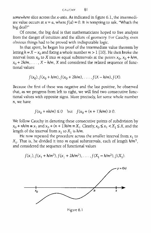
CAUCHY 81

somewhere slice across the x-axis. As indicated in figure 6.1, the intermedi­ate value occurs at x =a, where fCa) = O. It is tempting to ask. "What's thebig deal?"

Of course, the big deal is that mathematicians hoped to free analysisfrom the danger of intuition and the allure of geometry. For Cauchy, evenobvious things had to be proved with indisputable logic.

In that spint, he began his proof of the intermediate value theorem byletting h =X - Xo and fixing a whole number m > 1 [10]. He then broke theinterval from Xo to X into m equal subintervals at the points xo, Xo + him,Xo + 2h1m, ... , X - him, X and considered the related sequence of func­tional values:

fCxo),fCxo+ hlm),fCxo+ 2h1m), ... ,fCX - hlm),fCX).

Because the first of these was negative and the last positive, he observedthat, as we progress from left to right, we will find two consecutive func­tional values with opposite signs. More precisely, for some whole numbern, we have

fCxo+ nhlm) ~ 0 but fCxo+ Cn + 1)hlm) ~ O.

We follow Cauchy in denoting these consecutive points of subdivision byXo + nhlm == Xl and Xo + Cn + 1)hlm == Xl' Clearly, Xo ~ Xl < Xl ~ X, and thelength of the interval from Xl to Xl is him.

He now repeated the procedure across the smaller interval from Xl toXl' That is, he divided it into m equal subintervals, each of length him2 ,

and considered the sequence of functional values

y=f(x)

Figure 6.1

82 CHAPTER 6

Again, the leftmost value is less than or equal to zero, whereas the right­most is greater than or equal to zero, so there must be consecutive pointsx2 and X2a distance of hlm2 units apart, for which j(x2) ~ 0 and j(X2) ~ o.At this stage, we have Xo ~ Xl ~ X2< X2 ~ Xl ~ X. Those familiar with thebisection method for approximating solutions to equations should feelperfectly at home with Cauchy's procedure.

Continuing in this manner, he generated a nondecreasing sequenceXo ~ Xl ~ X2~ X3 ~ ... and a nonincreasing sequence··· ~ X3 ~ X2~Xl ~ X, where all the values j(xh) ~ 0 and j(Xh) ~ 0 and for which the gapXh - Xh=hlmh. For increasing k, this gap obviously decreases toward zero,and from this Cauchy concluded that the ascending and descendingsequences must converge to a common limit a. In other words, there is apoint a for which lim Xh = a = lim X h.

h~~ h~~

We pause to comment on this last step. Cauchy here assumed a ver-sion of what we now call the completeness property of the real numbers.He took it for granted that, because the terms of the sequences {Xh} and{Xh } grow arbitrarily close to one another, they must converge to a com­mon limit. One could argue that his belief in the existence of this point ais as much a result of unexamined intuition as simply believing the inter­mediate value theorem in the first place. But such a judgment may beoverly harsh. Even if Cauchy invoked an untested hypothesis, he had atleast pushed the argument much deeper toward the core principles. If hefailed to clear the path of all obstacles, he got rid of most of the brushunderfoot.

To finish the argument, Cauchy stated (without proof) that the pointa falls within the original interval from Xo to X, and then he used the con­tinuity of j to conclude, in modern notation, that

j(a) = j [lim Xh] = lim j(xh) ~ 0 andh~oo h~oo

j(a) = j[lim xh] = lim j(Xh) ~ o.h~~ k~~

In Cauchy's words, these inequalities established that "the quantityj(a) ... cannot differ from zero." He had thus proved the existence of anumber a between Xand X for which j(a) =O. The general version of theintermediate value theorem, namely that a continuous function takes allvalues betweenj(xo) andj(X), follows as an easy corollary.

This was a remarkable achievement. Cauchy had, for the most part,succeeded in demonstrating a "self-evident" principle by analytic methods.

CAUCHY 83

As Judith Grabiner observed, "though the mechanics of the proof are sim­ple, the basic conception of the proof is revolutionary. Cauchy trans­formed the approximation technique into something entirely different: aproof of the existence of a limit" [11].

THE MEAN VALUE THEOREM

We now turn to another staple of the calculus, the mean value theo­rem for derivatives [12]. In his Calcul infinitesimal, Cauchy began with apreliminary result.

Lemma: If, for a function f continuous between Xo and X, one lets A be thesmallest and B be the largest value that l' takes on this interval, then

A~f(X)- fCxo)~B.

X-xo

Proof: We note that Cauchy's reference to l'-and thus his unstatedassumption that f is differentiable-would of course guarantee thecontinuity of f. Moreover, he assumed outright that the derivativetakes a greatest and least value on the interval [xo, X]. A modernapproach would treat these hypotheses with more care.

If his statement seems peculiar, his proof began with a now­familiar ring, for Cauchy introduced two "very small numbers" 0 andE. These were chosen so that, for all positive values of i < 0 and for anyx between Xo and X, we have

f 'C ) fCx + i) - fCx) f'C)X - E < < X + E.

i(3)

Here Cauchy was assuming a uniformity condition for his choiceof o. The existence of the derivative certainly means that, for any E> 0and for any fixed x, there is a 0> 0 for which the inequalities of (3)hold. But such a 0 depends on both E and the particular point x.Without additional results or assumptions, Cauchy could not justifythe choice of a single 0 that simultaneously works for all x throughoutthe interval.

Be that as it may, he next subdivided the interval by choosingpoints

Xo < Xl < x2 < ... < xn- l < X,

84 CHAPTER 6

where Xl - X O, X2 - Xl' ... , X - xn- 1 "have numerical values lessthan 0." For these subdivisions, repeated applications of (3) and thefact that A ~ j'ex) ~ B imply that

feX) - fex )A - £ < j'exn- 1) - £ < n-1 < j'exn- 1) + £ < B+ £.

X - X n- 1

Cauchy then observed that, "if one divides the sum of thesenumerators by the sum of these denominators, one obtains a meanfraction which is ... contained between the limits A - £ and B+ £."

Here he was using the fact that, if bk > 0 for k =1, 2, ... , n and if

n / nC < :: < D for all k, then C <t ak t bk < D as well. Applying

this result to the inequalities above, he found that

feX) - fex o)which telescoped to A - £ < < B+ £. Cauchy ended the

X -xoproof WIth the statement that, "as this conclusion holds however small

be the number £, one can affirm that the expression [fex) - fe xo)]X- Xo

will be bounded between A and B." Q.E.D.

This is an interesting argument, one that stumbles over the issue ofuniformity yet demonstrates a genius in working WIth inequalities andemplOying the now-ubiquitous £ and 0 to reach its desired conclusion. Noone would confuse this level of generality and rigor with something fromthe early days of Newton and Leibniz.

Cauchy then used the lemma to prove his mean value theorem.

CAUCHY 85

Theorem: If the function f and its derivativel' are continuous between Xoand X, then for some () between 0 and 1, we have

Proof: The assumed continuity off' guarantees, by the general version ofthe intermediate value theorem, thatl' must take any value between itsleast (A) and its greatest (B). But according to the lemma, the number

f(X) - f(xo) . h " d" 1 d C h ""'--'---'----'''-'---'''- IS one suc mterme late va ue, an so, as auc y put It,X - X o

"there exists between the limits 0 and 1 a value of () sufficient to satisfythe equation

f(X) - f(x o) =1'[xo

+ ()(X - xo)]."

X - X o(4)

Q.E.D.

The conclusion in (4) differs from what we find in a modern textbookonly in the notational convention that replaces Cauchy's X o + ()(X - xo) byour c, where of course 0 < () < 1 implies X o < c < X.

So, this is the mean value theorem for derivatives, albeit proved underCauchy's assumption that the derivative is continuous, an assumptionmade to guarantee thatl' takes all intermediate values between A and B. Infact, this assumption is unnecessary, and modern proofs of the mean valuetheorem get along quite nicely without it. Moreover, it turns out thatderivatives take intermediate values whether or not they are continuous, astriking result we shall prove in chapter 10.

In the 1820s, these finer points were unclear, and Cauchy's insight,significant for its time, would not be the final word. Nevertheless, he hadidentified the mean value theorem as central to a rigorous development ofthe calculus, a position it retains to this day.

INTEGRALS AND THE FUNDAMENTAL THEOREM OF CALCULUS

Like Cauchy's approach to limits, his definition of the integral wouldreverberate through the history of calculus. We recall that Leibniz haddefined the integral as a sum of infinitely many infinitesimal summands

and chose the notation Jto suggest this. Strange as it may seem, by 1800

86 CHAPTER 6

integration was no longer perceived in this light. Rather, it had come tobe regarded primarily as the inverse of differentiation, occupying a sec­ondary position in the pantheon of mathematical concepts. Euler, forinstance, began his influential three-volume text on integral calculus withthe following:

Definition: Integral calculus is the method of finding, from agiven differential, the quantity itself; and the operation which pro­duces this is generally called integration. [13]

Euler thought of integration as dependent upon, and hence subservientto, differentiation.

Cauchy disagreed. He believed the integral must have an independentexistence and defined it accordingly. He thereby initiated a transformationthat, as the nineteenth century wore on, would catapult integration intothe analytic spotlight.

He began with a function j continuous on the interval between Xo

and X [14]. Although continuity was critical to his definition, Cauchypointedly did not assume that j was the derivative of some other func­tion. He subdivided the interval into what he called "elements" Xl - XO,

X2 - Xl' X3 - X 2 , ... , X - Xn- l and let

5 =(Xl - xo) j(xo) + (x2 - Xl) j(x l ) + (X3 - X 2) j(x2)

+ ... + (X - Xn- l ) j(xn- l ).

We recognize this as a sum of left-hand rectangular areas, but in his CalculinfiniteSimal, Cauchy made no mention of the geometry of the situationnor did he provide the now-customary diagram. He did, however, observethat "the quantity 5 clearly depends on: (1) the number n of elements intowhich we have divided the difference X - xo; (2) the values of these ele­ments and, as a consequence, the mode of division adopted." Further, heclaimed that "it is important to note that, if the numerical values of theelements differ very little and the number n is quite large, then the mannerof division will have an imperceptible effect on the value of 5."

Cauchy gave an argument in support of this last assertion, one thatassumed uniform continuity-"one 0 fits all"-without recognizing it. Inthis way, he believed he had proved the following result:

If we decrease indefinitely the numerical values of these elements[that is, of Xl - xo, x2 - Xl' X3 - X 2 , , X - xn- l ] while augment-ing their number, the value of 5 ends by attaining a certainlimit that depends uniquely on the form of the function j(x) and

CAUCHY 87

the extreme values Xo and X attained by the variable x. This limitis what we call a definite integral.

He followed Joseph Fourier (1768-1830) in adopting r j(x)dx as "themost simple" notation for the limit in question. Xo

Cauchys definition was far from perfect, in large measure because itapplied only to continuous functions. Still, it was a highly significantdevelopment that left no doubt about two critical points: (1) the integralwas a limit and (2) its existence had nothing to do with antidifferentiation.

As was his custom, Cauchy used the definition to prove basicresults. Some were general rules, such as the fact that the integral of thesum is the sum of the integrals. Others were specific formulas like

r xdx = X2

- x~ or r dx = In(~). And Cauchy established that,Xo 2 Xo x X o

for j continuous, there exists a value of ebetween 0 and 1 for which

Jx j(x)dx = (X - xo)j[xo + e(X - xo)]. (5)Xo

Readers will recognize this as the mean value theorem for integrals.Only then, having come this far without even mentioning derivatives,

was Cauchy ready to bind together the great ideas of differentiation andintegration. The unifying result is what we call the fundamental theoremof calculus. As one of the great theorems in all of mathematics, proved byone of the great analysts of all time, it surely deserves our attention [15].

As usual, Cauchy began with a continuous function j, but this time, inconsidering its integral, he let the upper limit of integration vary. That is,

he defined the function <I>(x) =r j(x)dx, although in the interest ofXo

clarity we now would write <I>(x) = JX j(t)dt. Cauchy argued thatXo

Jx+

a JX<I>(x + a) - <I>(x) = j(x)dx - j(x)dxXo Xo

=s: j(x)dx + J:+a j(x)dx - s: j(x)dx

Jx+a

= x j(x)dx.

Moreover, by (5), there exists ebetween 0 and 1 for which

Jx +ax j(x)dx = (x + a - x)j[x + e(x + a - x)] =a j(x + ea).

In short, <I>(x + a) - <I>(x) =aj(x + ea) for some value of e.

88 CHAPTER 6

To Cauchy, this last equation showed that <I> was continuous becausean infinitely small increase in x produces an infinitely small increase in <1>.Or, as we might put it,

lim[<I>(x + a) - <I>(x)] = lim af(x + ea) = lim a . lim f(x + ea)a-70 a-70 a-70 a-70

= lim a . f(limlx + ea]) =o· f(x) =0,a-70 a-70

where the continuity off at x implies ~~f(x + ea) = f(x). Consequently,

lim <I>(x + a) = <I>(x) and so <I> is continuous at x.a-70

But Cauchy was after bigger game, for it also followed that

'() l' [<I>(X + a) - <I>(X)] l' a f(x + ea)<I> x = 1m = Im----=:...---a-70 a a-70 a

= lim f(x + ea) = f(x).a-70

Just to be sure no one missed the point, Cauchy rephrased this as

d fX- f(x)dx = f(x).dx Xo

(6)

This is the "first version" of the fundamental theorem of calculus. In equa­tion (6), the inverse nature of differentiation and integration jumps rightoff the page.

Having differentiated the integral, Cauchy next showed how to inte­grate the derivative. He began with a simple but important result that hecalled a "problem."

Problem: If w is a function whose derivative is everywhere zero, then w isconstant.

Proof: We fix Xo in the function's domain. If x is another point in thedomain, the mean value theorem (4) guarantees a ebetween 0 and 1such that

w(x) - w(xo) _ 'I e( - )] - 0-----"- - w Xo + x Xo - ,x - Xo

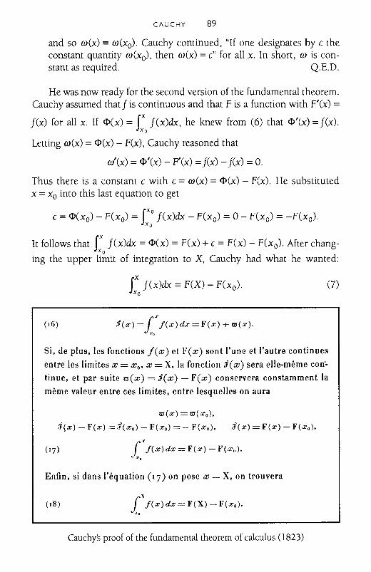
CAUCHY 89

and so w(x) =w(xo). Cauchy continued, "If one designates by e theconstant quantity w(xo), then w(x) = e" for all x. In short, w is con­stant as required. Q.E.D.

He was now ready for the second version of the fundamental theorem.Cauchy assumed that f is continuous and that F is a function with F'(x) =f(x) for all x. If <1>(x) = fX f(x)dx, he knew from (6) that <1>'(x) =f(x).

Xo

Letting w(x) =<1>(x) - F(x), Cauchy reasoned that

w'(x) = <1>'(x) - F'(x) =f(x) - f(x) =o.

Thus there is a constant e with e = w(x) = <1>(x) - F(x). He substitutedx =Xo into this last equation to get

fxoe = <1>(xo) - F(xo) = f(x)dx - F(xo) = 0 - F(xo) = -F(xo).

Xo

It follows that fX f(x)dx = <1>(x) = F(x) + e = F(x) - F(xo). After chang-Xo

ing the upper limit of integration to X, Cauchy had what he wanted:

fx f(x)dx = F(X) - F(xo).Xo

j(x) =1" lex) d.r =F(x) + m(x).T,

(7)

Si, de plus, les fonctions f(x) el F(x) sont l'une et l'autre continues

entre les limites x = X o' x = X, la fonction ~(x) sera elle-meme con"­

tinue, et par suite cr(x) = 3(X) - F(x) conservera constamment la

memo valeur entre ces limites, entre lesquelles on aura

m(x) = m(xo),

.1(x) - F(x) = i(xo) - F(xo) = - F(xo), i(x) = F(x) - F(xo)'

(17) jr/(X)dX = F(x) - F(xo).",

Enfin, si dans l'equation (17) on pose x = X, on trouvera

IX/(X) dx = F(X) - F(xo)..,Cauchy's proof of the fundamental theorem of calculus (823)

90 CHAPTER 6

To see the inverse relationship, we need only replace f(x) by F'(x) and

write (7) as JX F'(x)dx = F(X) - F(xo)' This version of the fundamentalXo

theorem integrates the derivative, thereby complementing its predecessor.So, when integrating a continuous function f across the interval from

Xo to X, we can short-circuit Cauchys intricate definition with its "ele­ments" and sums and limits provided we find an antiderivative F. In thishappy circumstance, evaluating the integral becomes nothing more thansubstituting Xo and X into F. One could argue that (7) represents the great­est shortcut in all of mathematics.

Although the fundamental theorem is a fitting capstone to any rigorousdevelopment of calculus, we end this chapter in yet another comer of analy­sis where Cauchy made a significant impact: the realm of infinite series.

Two CONVERGENCE TESTS

Like Newton, Leibniz, and Euler before him, Cauchy was a master ofinfinite series. But unlike these predecessors, he recognized the need totreat questions of convergence/divergence with care, lest divergent serieslead mathematicians astray. If Cauchy held such a position, it seemedincumbent upon him to supply tests for convergence, and on this front hedid not disappoint.

First we must say a word about Cauchys definition of the sum of aninfinite series. Earlier mathematicians, who could be amazingly clever inevaluating specific series, tended to treat these holistically, as single expres­sions that be~ved more or less like their finite counterparts. To Cauchy, the

meaning of L Uk was more subtle. It required a precise definition in orderk=O

to determine not only its value but its very existence.His approach is now familiar. Cauchy introduced the sequence of

partial sumsn-I

51 = uo, 52 = Uo + uI , 53 = Uo+ ul + u2 , and generally 5n = L Uk'

k=O

Then the value of the infinite series was defined to be the limit of thisn-l

sequence, that is, L Uk == lim 5n = lim L Uk, provided the limit exists,k=O n~oo n~oo k=O

in which case "the series will be called convergent and the limit ... will be

CAUCHY 91

called the sum of the series" [16]. As he had done with derivatives andintegrals, Cauchy erected a theory of infinite series upon the bedrock oflimits.

It was an ingenious idea, although in the process Cauchy committedan error of omission. From time to time, he asserted the existence of thelimit of a sequence of partial sums based on the fact that the partial sumsgrew ever closer to one another. By this last statement he meant that, forany e> 0, there is an index N so that the difference between SN and SN+k isless than e for all k ~ 1. In his honor, we now call a sequence with thisproperty a "Cauchy sequence."

However, he offered no justification for the idea that terms growingarbitrarily close to one another must necessarily converge to some limit. Asnoted above, this condition is an alternative version of the completenessproperty, the logical foundation upon which the theory of limits, and hencethe theory of calculus, now rests. To modem mathematicians, complete­ness must be addressed either by deriving it from a more elementary defi­nition of the real numbers or by adopting it as an axiom. One could arguethat Cauchy more or less did the latter, although there is a differencebetween assuming something explicitly (as an axiom) and assuming itimplicitly (as a gaffe).

In any case, he treated as self-evident the fact that a Cauchy sequenceis convergent. There is an irony here, for we now attach his name to a con­cept he did not fully comprehend. But rather than diminish his status, thisirony reinforces our previous observation that difficult ideas take time toreach maturity

With that prologue, we now consider a pair of tests with whichCauchy demonstrated the convergence of infinite series. Both proofs arebased on the comparison test for a se;:ies of nonnegative terms, which~says

that if 0::; ak::; bk for all k and if ~>k converges, then so does Lak.k=O k=O

Today the comparison test is proved by means of the aforementionedcompleteness property, and it remains one of the easiest ways to establishseries convergence.

The first of our results, the root test, he stated in the following words.

Theorem: For the infinite series Uo+ u1 +u2 + u3 + ... + Uk + ..., find the

limit or limits to which the expression IUk IlIk = V1Uk I converges and letA be the greatest of these. Then the series converges if A< 1 anddiverges if A> 1 [17].

92 CHAPTER 6

Before proceeding, we should clarify a few points. For one, Cauchydid not use the absolute value notation, as we have. Rather, he talkedabout Ph as the "numerical value" or the "modulus" of uh and framed theroot test in terms of Ph' Of course, this is just a symbolic convention, not asubstantive difference.

Perhaps less familiar is his reference to the I\. as the "greatest" ofthe limits. Again, we now have a term for this, the limit supremum, and we

write I\. =limsup luhl 11k or I\. = lim Iuk IlIk in place of Cauchy's verbal

descnption.For readers unfamiliar with the concept, an example may be useful.

= 1 1 1 1Suppose we consider the infinite series L Uk =1+ - + - + - + - +

k=O 3 4 27 161 1 1-- + - +--+ ... ,where reciprocals of certain powers of 3 alternate

243 64 2187with those of certain powers of 2. We see that the series terms uo, u1, u2 ,

u3 , ... obey the pattern:

for k = 0, 1, 2, ... ,

for k = 0, 1, 2, ....

If we look only at terms with even subscripts, we find the limit of their

roots to be lim 2~1/22k =.!.., whereas if we restrict ourselves to termsk~= 2

with odd subSCripts, we have lim 2k+~1I32k+l =.!... In modern parlance,k~= 3

the sequence {Iuh 111k} has a subsequence converging to .! and another11 2

converging to "3' In this case, the greater is I\. = "2'Cauchy's proof of the root test in Calcul infinitesimal is virtually

identical to that found in a modern text. He began with the casewhere 0 < I\. < 1 and fixed a number J1 so that I\. < J1 < 1. His criticalobservation was that the "greatest values" of Iuhl llh "cannot approachindefinitely the limit I\. without eventually becoming less than J1." As aconsequence, he knew there was an integer m such that, for all k :2: m,

CAUCHY 93

we have Iuk I11k < J1 and so 1uk I < J1 k. He then considered the two infiniteseries

where the geometric series on the right converges becau~ J1 < 1. From the

comparison test, Cauchy deduced the convergence of LIUk I, and thus ofk=O

LUk as well. In short, if A. < 1, the series converges. It follows, for instance,k=O

1111111that the series 1+ - + - + - + - + -- + - +-- + . .. converges

3 4 27 16 243 64 2187because A. =1/2.

His proof of the divergence case (A. > 1) was analogous. To demonstratethe importance of the root test, Cauchy applied it to determine what we

00 j(k\O)now call the radius of convergence of the Maclaurin series L x k

,k=O k!

and from there a rigorous theory of power series was on its way.There are other tests of convergence scattered through Cauchys

collected works, such as the ratio test (credited to d'Alembert) and the

Cauchy condensation test [181. The latter begins WIth a series L Uk, wherek=O

Uo~ Ul ~ U2 ~ ••. ~ 0 is a nonincreasing sequence of positive terms. Cauchyproved that the original senes and the "condensed" series Uo + 2uj + 4u1 +8u y + ... + 2 k U 2k -1 + ... converge or diverge together. In this case, select-

ed multiples of a subcollection of terms tell us all we need to knowabout the behavior of the original infinite series. It seems too good to betrue.

We conclude this section with a lesser known convergence test fromCauchy's arsenal, one that 'demonstrates his endless fascination with thistopic [191.

Theorem: If i:Uk is a series of positive terms for which lim In(uk) = h > 1,k=l k---7OO In(llk)

then the series converges.

Proof: As with the root test, Cauchy sought a "buffer" between 1 and handso chose a real number a WIth 1 < a < h. This guaranteed the existence

In(uk ) -In(uk )a < --- = ---"-

In(l/k) In k

94 CHAPTER 6

In(uk )of a positive integer m so that In(l/k) > a for all k ~ m. From there, heobserved that

and so a In(k) < In( :k J1

Exponentiating both sides of this inequality, he deduced that kG < ­Uk

1 ~ 1and so Uk < -; for all k ~ m. But 1-; (which is now called a p-series)

k h=m k~

converges because a > 1, and so the origInal senes I Uk converges byk=I

the comparison test. Q.E.D.

~ In(k)As an example, consider1--,where p > 1. Cauchys test requires us

k=! kP

In[ln(k)/kP]to evaluate lim I ( k) , which suggests in tum that we first simplify the

k--+~ n 1/quotient:

In[ln(k)/kP] In[ln(k)] - pIn(k) In[ln(k)]In(lIk) = -lnCk) = - InCk) + p.

, ., . (In[lnCk)] ) . .By I HospItals rule, ~~ - InCk) + p = P> 1, establIshmg the conver-

~ In(k) ,gence of £..J-- by Cauchys test. It is a very nice result.

k=I kP

Before leaving Augustin-Louis Cauchy, we offer an apology and a pre-view. We apologize for a chapter that reads like a precis of an introductoryanalysis text. Indeed, there is no stronger testimonial to Cauchy's influ­ence than that his "greatest hits" are now the heart and soul of the subject.Building upon the idea of limit, he developed elementary real analysis in away that remains the model to this day. As Bell properly observed, Cauchystands at center stage, and it is for this reason that the present chapter isone of the books longest. It could hardly be otherwise.

This brings us to the preview. None of these accolades should sug­gest that, after Cauchy, the quest was finished. On at least three frontsthere was still work to be done, work that will occupy us in chapters tocome.

CAUCHY 95

First, his definitions could be made more general and his proofs morerigorous. A satisfactory definition of the integral, for instance, need not belimited to continuous functions, and the nagging issue of uniformity hadto be identified and resolved. These tasks would fall largely to the Germanmathematicians Georg Friedrich Bernhard Riemann and Karl Weierstrass,who in a sense supplied the last word on mathematical precision.

Second, Cauchy's more theoretical approach to continuity, differen­tiability, and integrability motivated those who followed to sort out theconnections among these concepts. Such connections would intriguemathematicians throughout the nineteenth century, and their resultingtheorems-and counterexamples-would hold plenty of surprises.

Finally, the need to understand the completeness property raisedquestions about the very nature of the real numbers. The answers to thesequestions, combined with the arrival of set theory, would change the faceof analysis, although no mathematician active in 1840 could know that arevolution lay just over the horizon.

But any mathematician active in 1840 would have known aboutCauchy. On this front, we shall give the last word to math historian CarlBoyer. In his classic study of the history of calculus, Boyer wrote, "Through[his] works, Cauchy did more than anyone else to impress upon the sub­ject the character which it bears at the present time" [20].

In a very real sense, all who followed are his disciples.

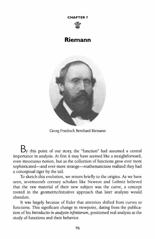
CHAPTER 7

Riemann

Georg Fnednch Bernhard Riemann

By this point of our story, the ~function ~ had assumed a centralimponance in analysis. At first it may have seemed like a straightfOlward,even innocuous notion, but as the colJection of functions grew ever moresophisticated-and ever more strange-mathematicians realized they hada conceptual tiger by the tail.

To sketch this evolution, we return briefly to the origins. As we haveseen, seventeenth century scholars like Newton and Leibniz believedthat the raw material of their new subject was the curve, a conceptrooted in the geometridintuitive approach that later analysts wouldabandon.

It was largely because of Euler that attention shifted from curves tofunctions. This significant change in viewpoint, dating from the publica­tion of his lntroducfio in analysin infinitorum, positioned real analysis as thestudy of functions and their behavior.

96

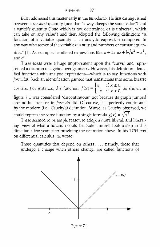
RIEMANN 97

Euler addressed this matter early in the Introductio. He first distinguishedbetween a constant quantity (one that "always keeps the same value") anda variable quantity ("one which is not determined or is universal, whichcan take on any value") and then adopted the following definition: "Afunction of a variable quantity is an analytic expression composed inany way whatsoever of the variable quantity and numbers or constant quan-

tities" fl]. As examples he offered expressions like a + 3z,az + b~a2 - Z2,and cZ.

These ideas were a huge improvement upon the "curve" and repre­sented a triumph of algebra over geometry. However, his definition identi­fied functions with analytic expressions-which is to say, functions withformulas. Such an identification painted mathematicians into some bizarre

h f f() {X if x ~ 0, h

corners. For instance, t e unction x = 'f 0 as s own in-x 1 x < ,

figure 7.1 was considered "discontinuous" not because its graph jumpedaround but because its formula did. Of course, it is perfectly continuousby the modern (i.e., Cauchy's) definition. Worse, as Cauchy observed, we

could express the same function by a single formula g(x) =R.There seemed to be ample reason to adopt a more liberal, and liberat­

ing, view of what a function could be. Euler himself took a step in thisdirection a few years after providing the definition above. In his 1755 texton differential calculus, he wrote

Those quantities that depend on others ... , namely, those thatundergo a change when others change, are called functions of

-1

Figure 7.1

98 CHAPTER 7

these quantities. This definition applies rather widely and includesall ways in which one quantity can be determined by others. [2]

It is important to note that this time he made no explicit reference to ana­lytic expressions, although in his examples of functions Euler retreated tofamiliar formulas like y = x2 .

As the eighteenth century became the nineteenth, functions wererevisited in the study of real-world problems about vibrating strings anddissipating heat. This story has been told repeatedly (see, for instance, [3]and [4]), so we note here only that a key figure in the evolving discussionwas Joseph Fourier. He came to believe that any function defined between-a and a (be it the pOSition of a string, or the distribution of heat in a rod,or something entirely "arbitrary") could be expressed as what we now calla Fourier series:

1 ~( nJrx . nJrx)j(x)=-ao+L. ahcos--+bhsm--,2 h=l a a

where the coefficients ah and bh are given by

1 fa nJrx 1 fa nJrxah = - j(x)cos--dx and bh = - j(x)sin-dx.a -a a a -a a

(1)

To insure that his readers were under no illusions about the level of gener­ality, Fourier explained that his results applied to "a function completelyarbitrary, that is to say, a succession of given values, subject or not to acommon law," and he went on to describe the values of y =j(x) as suc­ceeding one another "in any manner whatever, and each of them is givenas if it were a single quantity" [5].

This statement extended the "late Euler" pOSition that functions couldtake values at will across different points of their domain. On the otherhand, it was by no means clear that the formulas in (1) always hold. Thecoefficients ah and bh are integrals, but how do we know that integrals ofgeneral functions even make sense? At least implicitly, Fourier had raisedthe question of the existence of a definite integral, or, in modern terminol­ogy, of whether a function is or is not integrable.

As it turned out, Fourier had badly overstated his case, for not everyfunction can be expressed as a Fourier series nor integrated as required by(1). Further, in practice he restricted himself, as had Euler before him, toexamples that were fairly routine and well behaved. If the concept of a truly"arbitrary" function were to catch on, someone would have to exhibit one.

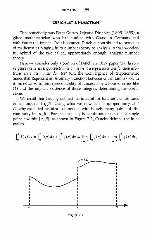
RIEMANN 99

DIRICHLET'S FUNCTION

That somebody was Peter Gustav Lejeune-Dirichlet 0805-1859), agifted mathematician who had studied with Gauss in Germany andwith Fourier in France. Over his career, Dirichlet contributed to branchesof mathematics ranging from number theory to analysis to that wonder­ful hybrid of the two called, appropriately enough, analytic numbertheory.

Here we consider only a portion of Dirichlets 1829 paper "Sur la con­vergence des series trigonometriques qui servent a representer une jonction arbi­trarie entre des Iimites donnees" (On the Convergence of TrigonometricSeries that Represent an Arbitrary Function between Given Limits) [6]. Init, he returned to the representability of functions by a Fourier series like0) and the implicit existence of those integrals determining the coeffi­cients.

We recall that Cauchy defined his integral for functions continuouson an interval [a, 13]. Using what we now call "improper integrals,"Cauchy extended his idea to functions with finitely many points of dis­continuity in [a, f31. For instance, if j is continuous except at a singlepoint r within [a, 13], as shown in Figure 7.2, Cauchy defined the inte­gral as

S:j(x)dx= {j(x)dx+ S: j(x)dx= li~tj(x)dx+ lirr:S: j(x)dx,t~r t~r

y=f(x)

~II,

a ,Figure 7.2

fJ

100 CHAPTER 7

provided all limits exist. If j has discontinuities at r j < r2 < r3 < ... < rn ,

we define the integral analogously as

f13 f't f'2 f'3 f13aj(x)dx= a j(x)dx+ '1 j(x)dx+ '2 j(x)dx+···+ 'nj(x)dx.

However, if a function had infinitely many discontinuities in the inter­val [a, f3], Cauchy's integral was of no use. Dirichlet suggested that a new,more inclusive theory of integration might be crafted to handle such func­tions, a theory connected to "the fundamental principles of infinitestimalanalysis." He never developed ideas in this direction nor did he show howto integrate highly discontinuous functions. He did, however, furnish anexample to show that such things exist.

"One supposes," he wrote, "that l/J(x) equals a determined constant cwhen the variable x takes a rational value and equals another constant dwhen the variable is irrational" [7]. This is what we now call Dirichlet'sfunction, written concisely as

(x) ={c if x is rational,l/J d if x is irrational. (2)

By the Fourier definition, l/J was certainly a function: to each x therecorresponded one y, even if the correspondence arose from no (obvious)aI1alytic formula. But the function is impossible to graph because of thethorough intermixing of rationals and irrationals on the number line:between any two rationals there is an irrational and vice versa. The graphof l/J would thus jump back and forth between c and d infinitely often aswe move through any interval, no matter how narrow. Such a thing cannotbe drawn nor, perhaps, imagined.

Worse, l/J has no point of continuity. This follows because of the sameintermixing of rationals and irrationals. Recall that Cauchy had definedcontinuity of l/J at a point x by lim[l/J(x + i) -l/J(x)] =O. As i moves toward

t~O

0, it passes through an infinitude of rational and irrational points. As aconsequence, l/J(x + i) jumps wildly back and forth, so that the limit inquestion not only fails to be zero but fails even to exist. Because this is thecase for any x, the function has no point of continuity.

The significance of this example was twofold. First, it demonstratedthat Fourier's idea of an arbitrary function had teeth to it. Before Dirichlet,even those who advocated a more general concept of function had not, inthe words of math historian Thomas Hawkins, "taken the implications ofthis idea seriously" [8]. Dirichlet, by contrast, showed that the world of

RIEMANN 101

functions was more vast than anyone had thought. Second, his examplesuggested an inadequacy in Cauchys approach to the integral. Perhaps inte­gration could be recast so as not to restrict mathematicians to integratingcontinuous functions or those with only finitely many discontinuity points.

It was Dirichlets brilliant student, the abundantly named GeorgFriedrich Bernhard Riemann (1826-1866), who took up this challenge.Riemann sought to define the integral without prior assumptions abouthow continuous a function must be. Divorcing integrability from continu­ity was a bold and provocative idea.

THE RIEMANN INTEGRAL

In his 1854 Habilitationsschrift, a high-level dissertation required of pro­fessors at German universities, RIemann stated the issue simply: "What is

one to understand by s: fex)dx?" [91. Assuming fto be bounded on [a, bl,

he proceeded with his answer.First, he took any sequence of values a < XI < x2 < ... < xn- I < b

within the interval [a, bl. Such a subdivision is now called a partition. Hedenoted the lengths of the resulting subintervals by °1 =XI - a, °2 =x2 - Xl'°3=X3 - X2, and so on up to On =b - Xn- l . Riemann next let EI , E2, ... , Enbe a sequence of values between 0 and 1; thus, for each Eh, the numberXh-I + Ehc\ lies between xh-I + 0 . c\ =Xh_1 and Xh-l + 1 . c\ =Xh_1 +(xh - Xh- I) =xh' In other words, Xh-I + Ehc\ falls within the subinterval[xh_l, xhl. He then introduced

5 = OJ(a + EI°1) + 02f(x I + E202) + 03f(x2 + E303)

+ ... + 0J(xn_1+ EnOn)·

The reader will recognize this as what we now (appropriately) call a Rie­mann sum. As illustrated in figure 7.3, it is the total of the areas of rectanglesstanding upon the various subintervals, where the kth rectangle has base c\and height f(Xh-1 + Ehc\)·

Riemann was now ready with his critical definition:

If this sum has the property that, however the c\ and Eh are cho­sen, it becomes infinitely close to a fixed value A as the c\ become

infinitely small, then we call this fixed value s: f(x)dx . If the sum

does not have this property, then f: f(x)dx has no meaning [10].

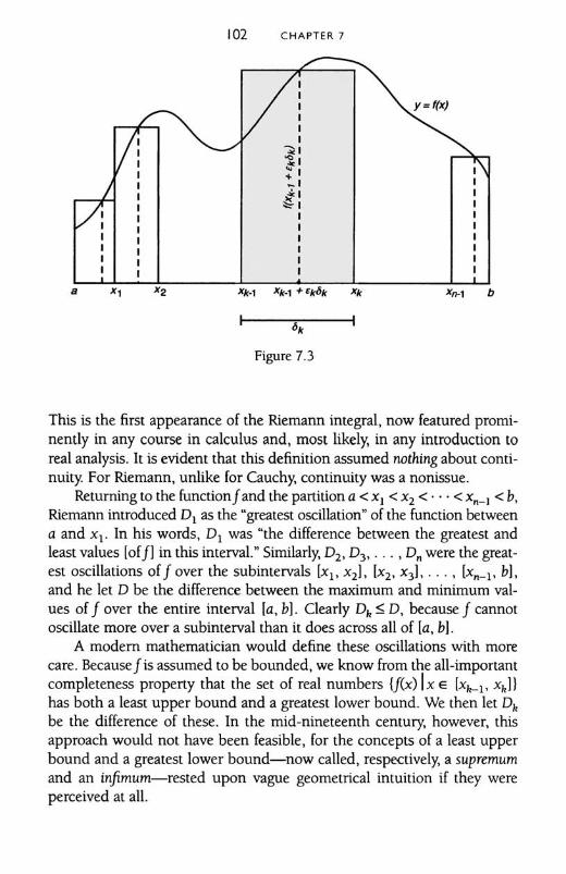
102 CHAPTER 7

,,, y= f(K),,,-.,1.,~,.,'::1'" ,,,,,,

a x, x, Xk·l Xk_l + ck6k Xx x~, b

'x

Figure 7.3

This is the first appearance of the Riemann integral, now featured promi­nently in any course in calculus and, most likely, in any introduction toreal analysis. It is evident that this definition assumed nothing about conti­nuity. For Riemann, unlike for Cauchy, continuity was a nonissue.

Returning to the functionf and the partition a < Xl < x2 < ... < Xn_ 1 < b,Riemann introduced D, as the "greatest oscillation" of the function betweena and Xl- In his words, D} was kthe difference between the greatest andleast values lof fJ in this interval." Similarly, D2• DJ , ... , Dn were the great­est oscillations off over the subintervals (Xl' X2), (X2' XJ1. ... , [Xn_I' bl,and he let D be the difference between the maximum and minimum val­ues of f over the entire interval (a, hI. Clearly D.. :S: 0, because f cannotoscillate more over a subinterval than it does across all of [a, hI.

A modem mathematician would define these oscillations with morecare. Becausef is assumed to be bounded, we know from the all·imponantcompleteness property that the set of real numbers Ij(x) Ix E [Xlt-l' x"JIhas both a least upper bound and a greatest lower bound. We then let D"be the difference of these. In the mid-nineteenth century, however, thisapproach would not have been feasible, for the concepts of a least upperbound and a greatest lower bound-now called, respectively, a supremumand an irif1mum-rested upon vague geometrical intuition if they wereperceived at all.

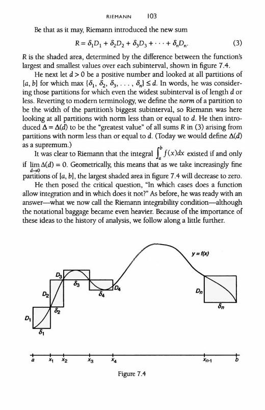
R.IEMANN 103

Be that as it may, Riemann introduced the new sum

R =olD} +°20 2+ 03D3 + ... + 0nDn. (3)

R is the shaded area, detennined by the difference between the functionslargest and smallest values over each subinterval, shown in figure 7.4.

He next let d > 0 be a positive number and looked at all partitions ofla, b] for which max (01' 02' °3"", 0n}:5 d. In words, he was consider­ing those partitions for which even the widest subinterval is of length d orless. Reverting to modern tenninology, we define the norm of a partition tobe the width of the partitions biggest subinterval, so Riemann was herelooking at all partitions with norm less than or equal to d. He then intro­duced li = li(d) to be the ~greatest value n of all sums R in (3) arising frompartitions with nann less than or equal to d. (Today we would define .6.(d)as a supremum.) b

It was clear to Riemann that the integral 1!(x)dx existed if and only

if lim li(d) = O. Geometrically, this means that as we take increasingly fine"-'0

partitions of la, bl, the largest shaded area in figure 7.4 will decrease to zero.He then posed the critical question, ~ln which cases does a function

allow integration and in which does it not?" As before, he was ready with ananswer-what we now call the Riemann integrability condition-althoughthe notational baggage became even heavier. Because of the importance ofthese ideas to the history of analysis, we follow along a little further.

• " "Figure 7.4

,~,

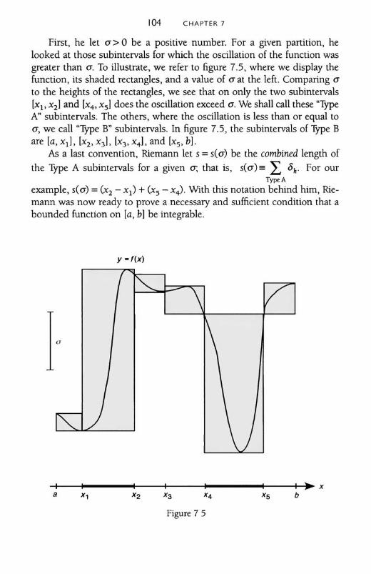
104 CHAPTER 7

First, he let a> 0 be a positive number. For a given partition, helooked at those subintervals for which the oscillation of the function wasgreater than G. To illustrate, we refer to figure 7.5. where we display thefunction, its shaded rectangles, and a value of G at the left. Comparing G

to the heights of the rectangles, we see that on only the two subintervals(Xl' x2] and (x4,x:d does the oscillation exceed G. We shall call these ~Type

A~ subintervals. The others, where the oscillation is less than or equal toG, we call ~Type B~ subintervals. In figure 7.5, the subintervals of Type Bare la, XII. (X2' X31. Ix), x4Land Ix:;, bl.

As a last convention, Riemann let s =sea) be the combined length of

the Type A subintervals for a given 0'; that is. S(G)= L 8•. For ourr"",,,

example, sea) = (x2 - Xl) + (xs - x 4). With this nalation behind him, Rie·mann was now ready to prove a necessary and sufficient condition that abounded function on la, bl be integrable.

y - {(xl

1""-\ /

" \

)1"'- \;a '.

Figure 7 5

b

RIEMANN 105

Riemann Integrability Condition: s: j(x)dx exists if and only if, for any

a> 0, the combined length of the Type A subintervals can be made assmall as we wish by letting d~ O.

Admittedly, there is a lot going on here. In words, this says that j is inte­grable if and only if, for any a no matter how small, we can find a norm sothat, for all partitions of la, b] having a norm that small or smaller, the totallength of the subintervals where the function oscillates more than a is neg­ligible. We examine Riemann's necessity and sufficiency proofs separately.

Necessity: If s: j (x)dx exists and we fix a value of a> 0, then

lims(a) = O.d-tO

Proof: Riemann began with a partition of unspecified norm d and consid­ered R=0PI + 02D2 + 03D3 + ... + 0nDn from (3). He noted that

R~ L 0kDk, because the summation on the right includes the Type AType A

terms and omits the others. But for each Type A subinterval, the oscil-lation ofj exceeds a; this is, of course, how the Type A subintervals areidentified in the first place. So, recalling the definition of s(a), we have

R~ L 0kDk ~ L 0ka = a· L Ok = a· s(a).Type A Type A Type A

On the other hand, R=0PI + 02D2 + 03D3 + ... + 0nDn ~ L\(d) because!l(d) is the greatest such value for all partitions having norm d or less.

Riemann combined this pair of inequalities to get a· s(a) ~ R ~

!led). Ignoring the middle term and dividing by a, he concluded that

(4)

Recall that, in proving necessity, he had assumed that j is integrable,and this in turn meant that !led) ~ 0 as d~ O. Because a was a fixed

!led)number, -- ~ 0 as well. It follows from (4) that, as d approaches

azero, the value of s(a) must likewise go to zero. Q.E.D.

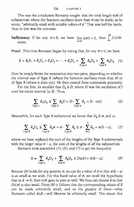
106 CHAPTER 7

This was the conclusion Riemann sought: that the total length s(a) ofsubintervals where the function oscillates more than a can be made, as hewrote, "arbitrarily small with suitable values of d." That was half the battle.Next in line was the converse.

Sufficiency: If for any a> 0, we have lim sea) = 0, then t J(x)dxexists. d--+O a

Proof: This time Riemann began by noting that, for any a> 0, we have

R = OlD) + oP2 + oP3 + ... + OPn = L ohDh + L ohDh' (5)Type A Type B

Here he simply broke the summation into two parts, depending on whetherthe interval was of Type A (where the function oscillates more than a) orof Type B (where it does not). He then treated these summands separately.

For the first, he recalled that Dh ~ D, where D was the oscillation ofJover the entire interval [a, b]. Thus,

L ohDh ~ L ohD = D· L Ok = D . sea). (6)Type A Type A Type A

Meanwhile, for each Type B subinterval we know that Dk ~ a, and so

n

L okDh ~ L oka = a· L oh ~ a· L oh = a(b - a), (7)Type B Type B Type B h=)

where we have replaced the sum of the lengths of the Type B subintervalswith the larger value b - a, the sum of the lengths of all the subintervals.

Riemann now assembled (5), (6), and (7) to get the inequality

R = L ohDh + L ohDh ~ Ds(a) + a(b - a). (8)Type A Type B

Because (8) holds for any positive a, we can fix a value of a so that a(b - a)is as small as we wish. For this fixed value of a, we recall the hypothesisthat as d -7 0, then sea) goes to zero as well. We thus can choose d so thatDs(a) is also small. From (8) it follows that the corresponding values of Rcan be made arbitrarily small, and so the greatest of these-whatRiemann called ~(d)-will likewise be arbitrarily small. This meant that

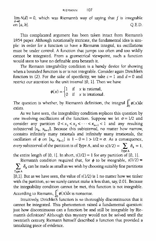
RIEMANN 107

lim !led) = 0, which was Riemann's way of saying that f is integrabled~O

on [a, b]. Q.E.D.

This complicated argument has been taken intact from Riemanns1854 paper. Although notationally intricate, the fundamental idea is sim­ple: in order for a function to have a Riemann integral, its oscillationsmust be under control. A function that jumps too often and too wildlycannot be integrated. From a geometrical viewpoint, such a functionwould seem to have no definable area beneath it.

The Riemann integrability condition is a handy device for showingwhen a bounded function is or is not integrable. Consider again Dirichlet'sfunction in (2). For the sake of specificity, we take c = 1 and d = °andrestrict our attention to the unit interval [0, 1]. Then we have

</J(x) ={I ~f x ~s rati~nal,° If x IS Irrational.

The question is whether, by Riemanns definition, the integral r</J(x)dx. 0

eXIsts.As we have seen, the integrability condition replaces this question by

one involving oscillations of the function. Suppose we let (J = 1/2 andconsider any partition °< Xl < x2 < ... < xn- I < 1 and any resultingsubinterval [Xk' Xk+I]. Because this subinterval, no matter how narrow,contains infinitely many rationals and infinitely many irrationals, theoscillation of </J on [xk' xk+I] is 1 - °= 1 > 1/2 = (J. As a consequence,

every subinterval of the partition is of Type A, and so s(1I2) = L Ok = 1,Type A

the entire length of [0, 1]. In short, s(1/2) = 1 for any partition of [0, 1].Riemanns condition required that, for </J to be integrable, s(1I2) =

L Ok can be made as small as we wish by choosing suitably fine partitionsType A

[0,1]. But as we have seen, the value of s(1/2) is 1 no matter how we tinkerwith the partition, so we surely cannot make it less than, say, 0.01. Becausethe integrability condition cannot be met, this function is not integrable.

According to Riemann, f: </J(x)dx is nonsense.Intuitively, Dirichlets function is so thoroughly discontinuous that it

cannot be integrated. This phenomenon raised a fundamental question:just how discontinuous can a function be and still be integrable by Rie­manns definition? Although this mystery would not be solved until thetwentieth century, Riemann himself described a function that provided atantalizing piece of evidence.

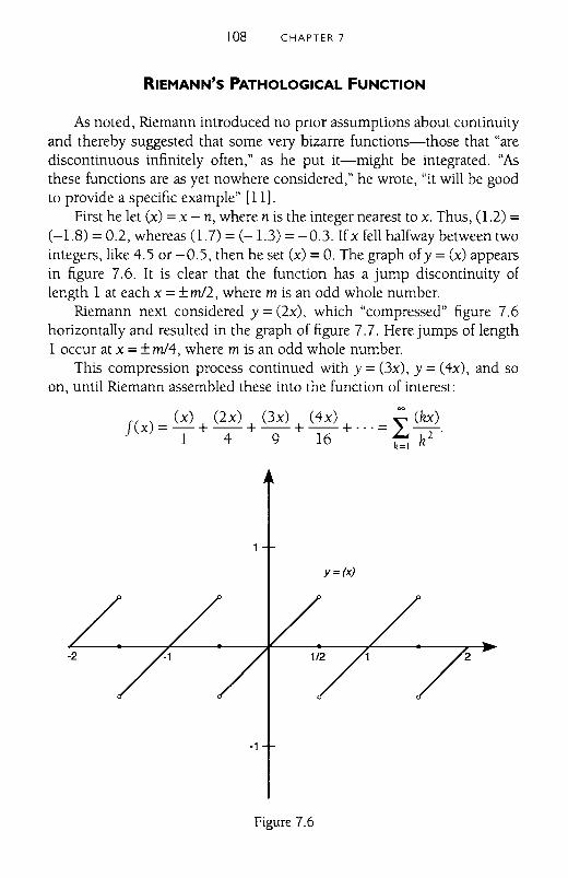
108 CHAPTER 7

RIEMANN'S PATHOLOGICAL FUNCTION

As noted, Riemann introduced no pnor assumptions about continuityand thereby suggested that some very bizarre functions-those that "arediscontinuous infinitely often," as he put it-might be integrated. "Asthese functions are as yet nowhere considered," he wrote, "it will be goodto provide a specific example" [lll.

First he let (x) = x - n, where n is the integer nearest to x. Thus, (1.2) =(-1.8) =0.2, whereas 0.7) =(-1.3) =-0.3. Ifx fell halfway between twointegers, like 4.5 or -0.5, then he set (x) =O. The graph ofy = (x) appearsin figure 7.6. It is clear that the function has a jump discontinuity oflength 1 at each x =±ml2, where m is an odd whole number.

Riemann next considered y = (2x), which "compressed" figure 7.6hOrizontally and resulted in the graph of figure 7.7. Here jumps of length1 occur at x =±ml4, where m is an odd whole number.

This compression process continued with y =Ox), y = (4x), and soon, until Riemann assembled these into the function of interest:

j(x) = (x) + (2x) + (3x) + (4x) + ... =i (~).1 4 9 16 n=! k

y=(x)

2

-1

Figure 7.6

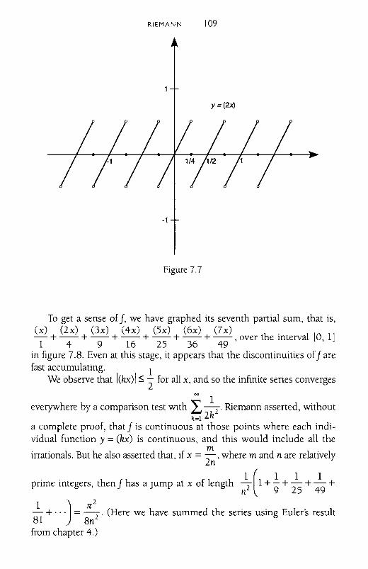
RIEMANN 109

y=(2x)

-1

Figure 7.7

To get a sense of j, we have graphed its seventh partial sum, that is,(x) (2x) Ox) (4x) (5x) (6x) (7x) h' 1 [ ]- + -- + -- + -- + -- + -- + -- over t e mterva 0 11 4 9 16 25 36 49' ,

in figure 7.8. Even at this stage, it appears that the discontinuities of j arefast accumulating. 1

We observe that IOve)1 ~ "2 for all x, and so the infinite series converges

00 1everywhere by a comparison test WIth L -2. Riemann asserted, without

k=12ka complete proof, that j is continuous at those points where each indi-vidual function y = (kx) is continuous, and this would include all the

mirrationals. But he also asserted that, if x =-, where m and n are relatively

2n

1 ( 1 1 1prime integers, then j has a Jump at x of length -2 1+ - + - + - +n 9 25 49

~ + 0 0 oJ = rc2

2. (Here we have summed the series using Euler's result

81 8nfrom chapter 4.)

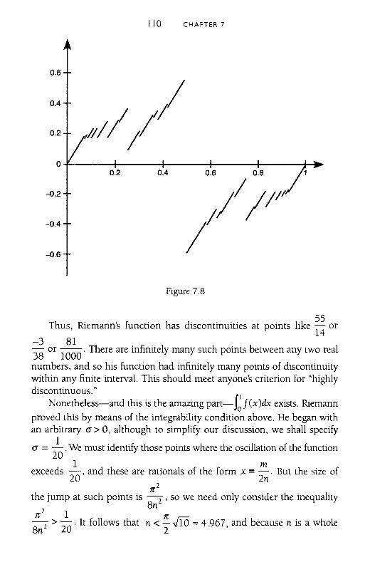
110 CHAPTER 7

0.6

0.4

0.2

// II111/ II

O+----~----+_---_+_---___ll__---+_~

-0.2

-0.4

-0.6

0.2 0.4

n 2 1-2 > -. It follows that8n 20

Figure 7.8

55Thus, Riemann's function has discontinuities at points like - or

14-3 8138 or 1000' There are infinitely many such points between any two real

numbers, and so his function had infinitely many points of discontinuitywithin any finite interval. This should meet anyone's criterion for "highlydiscontinuous."

Nonetheless-and this is the amazing part- f~ f (x)dx exists. Riemannproved this by means of the integrability condition above. He began withan arbitrary (J> 0, although to simplify our discussion, we shall specify

(J =~.We must identify those points where the oscillation of the function20

1 mexceeds -, and these are rationals of the form x =-. But the size of

20 2nn 2

the jump at such points is -2 ' so we need only consider the inequality8n

n <!!"'.Jl6 "" 4.967, and because n is a whole2

RIEMANN III

number, the only options are n = 1, 2, 3, or 4. When we note as well thatm

m and n have no common factors and that a ::; - ::; 1, we conclude that2n

there are only finitely many such candidates. In this case, the pointsIII 1 1 3

in [0, 1] where the function oscillates more than - are: -, -, -, -,-,1 5 2 3 5 7 20 8 6 4 3 8- - - - - and-2'8'3'4'6' 8'

Because we have only finitely many points to deal WIth, we can createa partition of [0, 1] that places each of these within a very narrow subin­terval, the total length of which can be as small as we wish. For instance,to include the eleven points above in subintervals with total length lessthan 1/100, we might begin our partition with

a< x = ~__1_ = 1249 < x = ~ + _1_ = 12511 8 10000 10000 2 8 10000 10000'

1thereby embedding the discontinuity at x = "8 in a subinterval of total

1251 1249 1 .length °1 =-- - -- =--. If we put equally narrow mtervals

10000 10000 5000

aoout each of the Type A points for a= ~, then s("!"') = 11 x (_1_)1 20 20 5000

<--.100

The critical issue here is the finite number of points where the oscilla­tion exceeds a given a. Riemann summarized the situation as follows: "Inall intervals which do not contain these jumps, the oscillations are lessthan a and ... the total length of the intervals that contain these jumpscan, at our pleasure, be made small" [12].

Riemann had constructed a function with infinitely many disconti­nuities in any interval yet that met his integrability condition. It was apeculiar creation, one that is now known as Riemann's pathologicalfunction, where the adjective carries the connotation of being, in somesense, "sick."

Of course, Riemann had not answered the question, "How discontin­uous can an integrable function be?" But he had shown that integrablefunctions could be stunningly discontinuous. To those critics who sneeredthat an example as weird as Riemann's was of no practical use, he offered apersuasive rejoinder: 'This topic stands in the closest association with the

112 CHAPTER 7

pnnciples of infinitesimal analysis and can serve to bring to these principlesgreater clarity and precision. In this respect, the topic has an immediateinterest" [13]. Riemann's pathological function had precisely this effect,even if it did proVIde a blow to the mathematical intuition. As we shall see,more intuition-busters were in store for analysts of the nineteenth century.

THE RIEMANN REARRANGEMENT THEOREM

To be sure, Riemann is best known for his theory of the integral, butwe end this chapter in a different corner of analysis, Wlth a Riemannianresult that may be less important than whimsical, but one that never ceasesto amaze the first-time student.

We begin by recalling the Leibniz series from chapter 2, namely,

1 1 1 11- - + - - - + - - .... Suppose we rearrange the terms of this series in

357 9the follOwing manner: take the first two positive terms followed by the firstnegative; take the next two positive terms followed by the second negative;and so on. After grouping this rearrangement into threesomes, we have

(1+.!. _.!.) +(1. +~ _1.) +(~+ ~ _~) +(~+ _1 _~)+....

5 3 9 13 7 17 21 11 25 29 15

(9)

A moment's thought reveals that the expressions in parentheses look like

111--+----- for k=I,2,3,4, ... ,8k - 7 8k - 3 4k - 1

d h b b· d· 24k - 11an t ese can e com me mto ---------(8k - 7)(8k - 3)(4k - 1)

Because k ~ 1, both the numerator and denominator of this last frac­tion must be positive, and so the value of each threesome in (9) will bepositive as well. We thus can say the following about the rearranged series:

( 1+.!. - 1.) +(.!. +~ -.!.) +(~+ ~ -~)+(~+ ~ -~)+...5 3 9 13 7 17 21 11 25 29 15

( 1 1) 132: 1+- - - +0 +0 +0 +0 +... = - = 0.8666...5 3 15

proved that the original series

We are left with an inescapable

RIEMANN 113

On the other hand, Leibniz had1 1 1 1 1C

1- - + - - - + - - ... = - "" 0.7854.3 5 7 9 4

conclusion: the rearranged series, whose sum has been shown to exceed0.8666, cannot converge to the same number as the original By alteringnot the terms of the series but their position, we have changed the sum.This seems mighty odd.

Actually, it gets worse, for Riemann showed how the Leibniz seriescan be rearranged to converge to any number at all!

His reasoning is expedited by the introduction of some terminologyand a few well-known theorem~ As we saw, it was Cauchy who said what

it means for an infinite series L. Uk to converge. A general series may, ofk=l

course, include both positive and negative terms, and this suggests that=

we disregard the signs and look at L.IUk I instead. If this latter seriesk=l

converges, we say that L. Uk converges absolutely. If L. Uk converges butk~ k~

L.1Uk I does not, the original series is said to converge conditionally.k=l

As an example, we return to the original series of Leibniz. It sums to

!!.- but the related series of absolute values diverges because4'

1111 111111+-+-+-+-+··· ~ -+-+-+-+-+ ...

3579 246810

= ~[1 +~+ ~ +~+~+ ... ]2 2 3 4 5 '

where we recognize the divergent harmonic series in the brackets. Thismeans that Leibnizs series is conditionally convergent.

It is customary when dealing with series of mixed signs to considerthe positives and the negatives separately. Following Riemann's notation,we write a series as (a l + a2 + a3 + a4 + ...) + (- bl - b2 - b3 - b4 - .••),

where all the ah and bh are nonnegative. Riemann knew that if the original= =

series converged absolutely, then both of the series L. ak and L. bkk=l k=l

converge; if the original series diverged, then one of L.ak and L.bkk=l k=l

114 CHAPTER 7

diverges to infinity; and if the original converged conditionally, then both00 00

Lahand Lbh diverge to infinity.h=1 k=1

It was Dirichlet who showed that any rearrangement of an absolutelyconvergent series must converge to the same sum as the original [14).For absolutely convergent series, repositioning the terms has no impactwhatever.

But for conditionally convergent series, we reach a dramatically differ­ent conclusion: if a series converges conditionally, it can be rearranged toconverge to whatever number we wish. With some alliterative excess, wemight call this Riemann's remarkable rearrangement result. Here is theidea of his proof.

Letting C be a fixed number-our "target," so to speak-Riemannbegan thus: "One alternately takes sufficiently many positive terms of theseries that their sum exceeds C and then sufficiently many negative termsthat the (combined) sum is less than C [15). To see what he was gettingat, we stipulate that our target C is positive. Starting with the positiveterms, we find the smallest m so th:t al + a2 + a3 + ... + am > C. There

surely is such an index because L ah diverges to infinity. One nexth=1

considers the negative terms and chooses the smallest n so that al + a2 +a3 + ... + am - bI - b2 - ••• - bn < C. Again, we know such an index

00

exists because the divergent series L bk must eventually exceed (a l + a2 +h=1

a3 + ... + am) - C. But al + a2 + a3 + ... + am - bl - b2 - ... - bn is arearrangement of terms of the original series whose sum can be no furtherfrom ethan bn" The process is then repeated, adding some ah and sub­tracting some bk so that the difference between C and this sum of theserearranged terms is less than some bp. Because the original series con­verges, we know its general term goes to zero, so lim br = 0 as well. The

r~oo

series rearranged by his alternating scheme will converge to C as claimed.It is quite wonderful.

To illustrate, suppose we sought a rearrangement of Leibnizs seriesthat would converge to, say, 1.10. We would begin with sufficiently many

1positive terms to exceed this: 1+ '5 = 1.2 > 1.10. Then we would subtract

a negative term to bring us below 1.10:

(1 + ~)-l = 0.8666· .. < 1.10.

RIEMANN 115

Then we add back some positive terms until we again surpass 1.10, thenbounce back with some negatives, and so on. With this recipe, therearranged Leibniz series that converges to 1.10 will begin as follows:

Once seen, Riemann's argument seems self-evident. Nonetheless, hisrearrangement theorem demonstrates in dramatic fashion that summinginfinite senes is a tricky business. By simply rearranging the terms we candrastically alter the answer. As has been observed previously, the study ofinfinite processes, which is to say analysis, can carry us into deep waters.

With that, we leave Georg Friedrich Bernhard Riemann, although nojourney through nineteenth century analysis can leave him for long. Morethan anyone, he established the integral as a primary player in the calcu­lus enterprise. And his ideas would serve as the point of departure forHenri Lebesgue, who, as we shall see in the book's final chapter, picked upwhere Riemann left off to develop his own revolutionary theory of inte­gration.

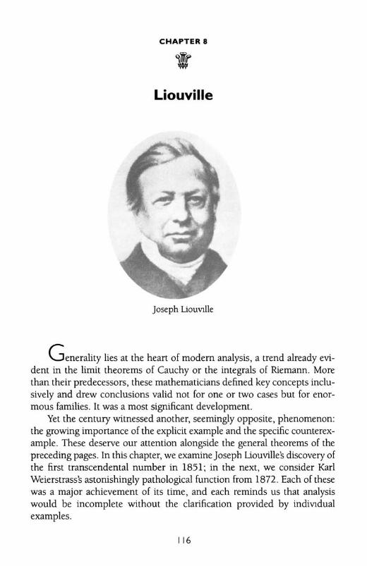
CHAPTER a

Liouville

Joseph LiouVllle

Generality lies at the heart of modem analysis, a trend already evi­dent in the limit theorems of Cauchy or the integrals of Riemann. Morethan their predecessors, these mathematicians defined key concepts inclu­sively and drew conclusions valid not for one or two cases but for enor~

mous families. It was a most significant development.Yet the century witnessed anOlher, seemingly opposite, phenomenon:

the growing importance of the explicit example and the specific counterex­ample. These deserve our auention alongside the general theorems of thepreceding pages. In this chapter, we examineJoseph Liouville's discovery ofthe first transcendental number in 1851; in the next, we consider KarlWeierstrass's astonishingly pathological function from 1872. Each of thesewas a major achievement of its time, and each reminds us that analysiswould be incomplete without the clarification provided by indivtdualexamples.

116

LIOUVILLE 117

To study transcendentals, we need some background on where theproblem originated, how it was refined over the decades, and why its res­olution was such a grand achievement. We start, as did calculus itself, inthe seventeenth century.

THE ALGEBRAIC AND THE TRANSCENDENTAL

It appears to have been Leibniz who first used the term "transcenden­tal" in a mathematical classification scheme. Writing about his newlyinvented differential calculus, Leibniz noted its applicability to fractions,roots, and similar algebraic quantities, but then added, "It is clear that ourmethod also covers transcendental curves-those that cannot be reducedby algebraic computation or have no particular degree-and thus holds ina most general way" [1]. Here Leibniz wanted to separate those entitiesthat were algebraic, and thus reasonably straightforward, from those thatwere intrinsically more sophisticated.

The distinction was refined by Euler in the eighteenth century. In hisIntroductio, he listed the so-called algebraic operations as "addition, sub­traction, multiplication, division, raising to a power, and extraction ofroots," as well as "the solution of equations." Any other operations weretranscendental, such as those involving "exponentials, logarithms, andothers which integral calculus supplies in abundance" [2]. He even wentso far as to mention transcendental quantities and gave as an example "log­anthms of numbers that are not powers of the base," although he provid­ed no airtight definition nor rigorous proof [3].

Our mathematical forebears had the right idea, even if they failed toexpress it precisely To them it was eVldent that certain mathematical objects,be they curves, functions, or numbers, were accessible via the fundamentaloperations of algebra, whereas others were sufficiently complicated to tran­scend algebra altogether and thereby earn the name "transcendental."

After contnbutions from such late eighteenth century mathematiciansas Legendre, an unambiguous definition appeared. A real number wassaid to be algebraic if it solved some polynomial equation with integercoefficients. That is, Xo is an algebraic number if there exists a polynomialP(x) =axn + bxn- l + cxn- 2 + ... + gx + h, where a, b, c, ... , g, and hareintegers and such that P(xo) =O. For instance, .J2. is algebraic because it isa solution ofx2 - 2= 0, a quadratic equation with integer coefficients. LessobVlously, the number .fi + V5 is algebraic for it solves x6 - 6x4 - 10x3 +l2x2 - 60x + 17 = O.

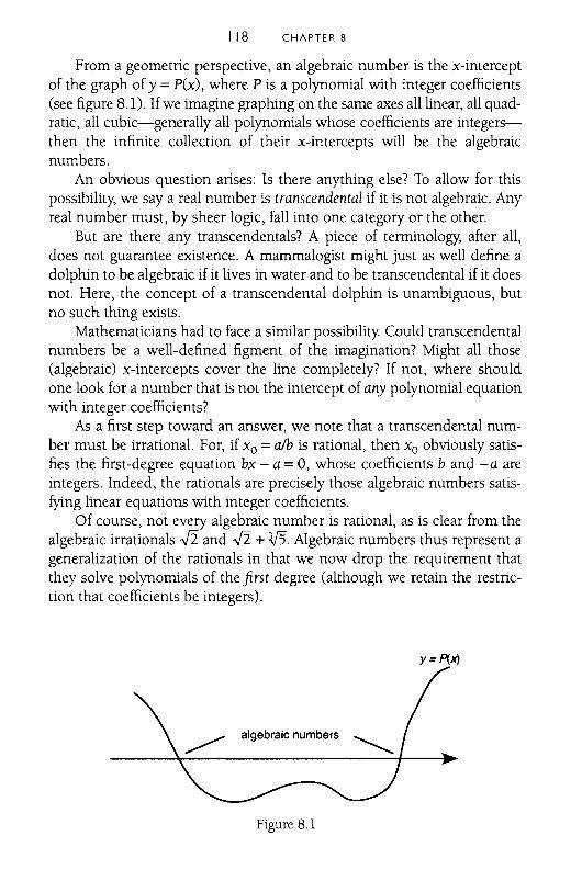
118 CHAPTER 8

From a geometric perspective, an algebraic number is the x-interceptof the graph of y =P(x), where P is a polynomial with integer coefficients(see figure 8.1). If we imagine graphing on the same axes all linear, all quad­ratic, all cubic-generally all polynomials whose coefficients are integers­then the infinite collection of their x-intercepts will be the algebraicnumbers.

An obvious question arises: Is there anything else? To allow for thispossibility, we say a real number is transcendental if it is not algebraic. Anyreal number must, by sheer logic, fall into one category or the other.

But are there any transcendentals? A piece of terminology, after all,does not guarantee existence. A mammalogist might just as well define adolphin to be algebraic if it lives in water and to be transcendental if it doesnot. Here, the concept of a transcendental dolphin is unambiguous, butno such thing exists.

Mathematicians had to face a similar possibility. Could transcendentalnumbers be a well-defined figment of the imagination? Might all those(algebraic) x-intercepts cover the line completely? If not, where shouldone look for a number that is not the intercept of any polynomial equationwith integer coefficients?

As a first step toward an answer, we note that a transcendental num­ber must be irrational. For, if Xo =alb is rational, then Xo obviously satis­fies the first-degree equation bx - a =0, whose coefficients b and -a areintegers. Indeed, the rationals are precisely those algebraiC numbers satis­fying linear equations with integer coefficients.

Of course, not every algebraiC number is rational, as is clear from thealgebraic irrationals .fi and .fi + VS. Algebraic numbers thus represent ageneralization of the rationals in that we now drop the requirement thatthey solve polynomials of the first degree (although we retain the restric­tion that coefficients be integers).

Y= P(x)

~ algebraic numbers -..............

Figure 8.1

LIOUVILLE 119

Transcendentals, if they exist, must lurk among the irrationals. Fromthe time of the Greeks, roots like -Ji were known to be irrational, and bythe end of the eighteenth century, the irrationality of the constants e and 7(

had been established, respectively, by Euler in 1737 and Johann Lambert(1728-1777) in 1768 [4]. But proving irrationality is a far easier task thanproving transcendence.

As we noted, Euler conjectured that the number log23 is transcenden­tal, and Legendre believed that 7( was as well [5]. However, beliefs of math­ematicians, no matter how fervently held, prove nothing. Deep into thenineteenth century, the existence of even a single transcendental numberhad yet to be demonstrated. It remained possible that these might occupythe same empty niche as those transcendental dolphins.

An example was provided at long last by the French mathematicianJoseph Liouville (1809-1882). Modern students may remember his namefrom Sturm-Liouville theory in differential equations or from Liouville'stheorem ("an entire, bounded function is constant") in complex analysis.He contributed significantly to such applied areas as electricity and ther­modynamics and, in an entirely different arena, was elected to the Assem­bly of France during the tumultuous year of 1848. On top of all of this, forthirty-nine years he edited one of the most influential journals in the his­tory of mathematics, onginally titled Journal de mathematiques pures etappliquees but often referred to simply as the Journal de Liouville. In thisway, he was responsible for transmitting mathematical ideas to colleaguesaround Europe and the world [6].

Within real analysis, Liouville is remembered for two significant discov­eries. First was his proof that certain elementary functions cannot have ele­mentary antiderivatives. Anyone who has taken calculus will rememberapplying clever schemes to find indefinite integrals. Although these mattersare no longer addressed with quite as much zeal as in the past, calculuscourses still cover techniques like integration by parts and integration by

partial fractions that allow us to compute such antiderivatives as Jx 2e-xdx =_x 2e-x

- 2xe-x- 2e-x +C or the considerably less self-evident

f ~dx 1 I Itanx -..)2 tan x + 11'" tan x = - n -------;====---.j8 tan x + ..)2 tan x + 1

+ ~ arctan (.J2tanXI + c.",2 1- tan x )

Note that both the integrands and their antiderivatives are composed offunctions from the standard Eulerian repertoire: algebraic, trigonometric,

120 CHAPTER 8

logarithmic, and their inverses. These are "elementary" integrals with "ele­mentary" antiderivatives.

Alas, even the most diligent integrator will be stymied in his or her questfor f ..Jsin x dx as a finite combination of simple functions. It was Liouvillewho proved in an 1835 paper why a closed-form answer for certain integralsis impossible. For instance, he wrote that, "One easily convinces oneself

JeX

by our method that the integral - dx, which has greatly occupiedx

geometers, is impossible in finite form" [7]. The hope that easy functionsmust have easy antiderivatives was destroyed forever.

In this chapter our object is Liouville's other famous contribution: aproof that transcendental numbers exist. His original argument came in1844, although he refined and simplified the result in a classic 1851 paper(published in his own journal, of course) from which we take the proofthat follows [8]. Before providing his example of a hitherto unseen tran­scendental, Liouville first had to prove an important inequality about irra­tional algebraic numbers and their rational neighbors.

LIOUVILLE'S INEQUALITY

As noted, a real number is algebraic if it is the solution to some polyno­mial equation with integer coefficients. Any number that solves one suchequation, however, solves infinitely many For instance, .J2 is the solution ofthe quadratic equation x2 - 2 =0, as well as the cubic equation x3 +x2 - 2x- 2 = (x2 - 2)(x + 1) =0, the quartic equation x4 + 4x3 +x2 - 8x - 6=(x2 - 2)(x + l)(x + 3) =0, and so on. Our first stipulation, then, is that weuse a polynomial of minimal degree. So, for the algebraic number .J2, wewould employ the quadratic above and not its higher degree cousins.

Suppose that Xo is an irrational algebraic number. Following Liouville'snotation, we denote its minimal-degree polynomial by

P(x) =axn + bxn- l + CXn- 2 + ... +gx + h, (1)

where a, b, c, ... ,g, and h are integers and n ~ 2 (as noted above, if n = 1,the algebraic number is rational). Because P(xo) =0, the factor theoremallows us to write

P(x) = (x - xo) Q(x), (2)

where Q is a polynomial of degree n - 1. liouVIlle wished to estab­lish a bound upon the size of IQ(x)1, at least for values of x in the vicinityof xo' We give his proof and then follow it with a simpler alternative.

LIOUVILLE 121

Liouville's Inequality: If Xo is an irrational algebraic number withminimum-degree polynomial PCx) =axn+ bxn- 1 + cxn- 2+ ... +gx + hhaving integer coefficients and degree n ~ 2, then there exists a positive

real number A so that, if plq is a rational number in [xo- 1, Xo + 1], then

Proof: The argument has its share of fine points, but we begin with thereal polynomial Q introduced in (2). This is continuous and thusbounded on any closed, finite interval, so there exists an A > 0 Wlth

IQCx)1 ~A for all x in [xo -1,xo+ 1]. (3)

Now consider any rational number plq Wlthin one unit of xo, wherewe insist that the rational be in lowest terms and that its denominator bepositive (i.e., that q ~ 1). We see by (3) that IQCplq)j ~ A. We claim as well

that PCplq)"# 0, for otherwise we could factor PCx) = (x - ~JRCX)' and

it can be shown that R will be an Cn - l)st-degree polynomial

having integer coefficients. Then 0 = PCxo) =(xo- ~)RCXo) and yet

( Xo - ~) "# 0 Cbecause the rational plq differs from the irrational xo),

and we would conclude that RCxo) = O. This, however, makes Xo a rootof R, a polynomial with integer coefficients having lower degree thanP, in Vlolation of the assumed minimality condition. It follows that plqis not a root of PCx) = O.

Liouville returned to the minimal-degree polynomial in (1) anddefined J Cp,q) == qnPCp/q). Note that

JCp,q) =qnpCplq)

=qn[aCplqt + bCplqt-1 + cCplqt-2+ ... + gCplq) + h]

=apn + bpn-lq+ cpn-2q2 + ... + gpqn-l + hqn. (4)

From C4), he made a pair of simple but telling observations.

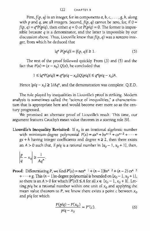
122 CHAPTER 8

First,j(p, q) is an integer, for its components a, b, e, ... , g, h, alongwith p and q, are all integers. Second,f(p, q) cannot be zero, for, if 0 =f(p, q) =qnp(plq), then either q =0 or P(plq) =O. The former is impos­sible because q is a denominator, and the latter is impossible by ourdiscussion above. Thus, Liouville knew that f(p, q) was a nonzero inte­ger, from which he deduced that

Iqn P(plq)1 = !f(p, q)1 ~ 1. (5)

The rest of the proof followed quickly. From (3) and (5) and thefact that P(x) =(x - xo) Q(x), he concluded that

Hence Iplq - xol ~ 1lAqn, and the demonstration was complete. Q.E.D.

The role played by inequalities in Liouvilles proof is striking. Modernanalysis is sometimes called the "science of inequalities," a characteriza­tion that is appropriate here and would become ever more so as the cen­tury progressed.

We promised an alternate proof of Liouville's result. This time, ourargument features Cauchys mean value theorem in a starring role [9].

Liouville's Inequality Revisited: If Xo is an irrational algebraic numberwith minimum-degree polynomial P(x) =axn+ bxn- 1 + exn- 2 + ... +gx + h having integer coefficients and degree n ~ 2, then there exists

an A > 0 such that, if piq is a rational number in [xo - 1, Xo + 1], then,

Proof: Differentiating P, we find P'(x) =naxn- 1 + (n - l)bxn- 2 + (n - 2) cxn-3

+ ... +g. This (n - 1)st-degree polynomial is bounded on [xo - 1, Xo + 1],so there is an A> 0 for which 1P'(x)1 ~ A for all x E [xo - 1, Xo + 1]. Let­ting plq be a rational number within one unit of Xo and applying themean value theorem to P, we know there exists a point e between Xoand plq for which

P(plq) - P(xo) = P'(e).plq - Xo

(6)

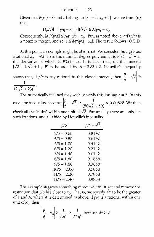
LIOUVILLE 123

Given that P(xo) =0 and e belongs to [xo - 1, Xo+ 1], we see from (6)that

IP(plq)I= Iplq - xol . 1P'(e)1 ~ Alplq - xol.

Consequently, Iqnp(plq)1 ~ Aqnlplq - xol. But, as noted above, qnp(plq) isa nonzero integer, and so 1 ~ Aqnlplq - xol. The result follows. Q.E.D.

At this point, an example might be of interest. We consider the algebraicirrational Xo = -ti. Here the minimal-degree polynomial is P(x) =x2 - 2,the derivative of which is P'(x) =2x. It is clear that, on the interval[-ti - 1, -ti + 1], P' is bounded by A = 2-ti + 2. Liouville's inequality

showsIthat, if plq is any rational in this closed interval, then I~ - .J21 ~

(2-ti + 2)q2 .

The numerically inclined may wish to verify this for, say, q =5. In this

case, the inequality becomes IE - -til ~ l "" 0.00828. We then5 (50 2 + 50)

check all the "fifths" within one unit of -ti. Fortunately, there are only tensuch fractions, and all abide by Liouville's inequality:

piS

315 =0.604/5 =0.80SIS = 1.006/5 =1.207/5 = 1.408/5 =1.609/5 = 1.80lOIS = 2.00IllS =2.2012/5 = 2.40

Ipl5 --til

0.81420.61420.41420.21420.01420.18580.38580.58580.78580.9858

The example suggests something more: we can in general remove therestriction that plq lies close to xo' That is, we specify A* to be the greaterof 1 and A, where A is determined as above. If plq is a rational within oneunit of xo, then

IE- xol ~ _1_ ~ _1_ because A* ~ A.q Aqn A* qn

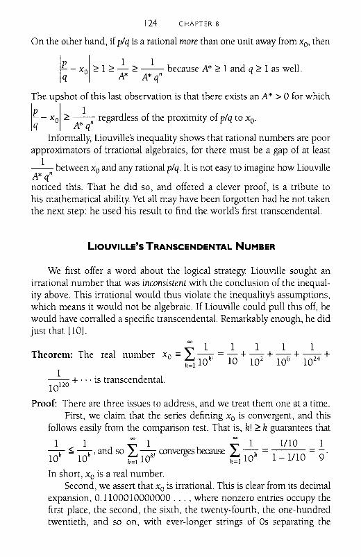
124 CHAPTER 8

On the other hand, if p/q is a rational more than one unit away from xo, then

IE. - xol ~ 1 ~ ~ ~ _1_ because A* ~ 1 and q ~ 1 as well.q A* A* qn

The upshot of this last observation is that there exists an A* > 0 for which

IE. - xol ~ _1_ regardless of the proximity of p/q to xo'q A* qn

Informally, Liouville's inequality shows that rational numbers are poorapproximators of irrational algebraics, for there must be a gap of at least

_1_ between Xoand any rational p/q. It is not easy to imagine how liouVIlleA* qnnoticed this. That he did so, and offered a clever proof, is a tribute tohis mathematical ability. Yet all may have been forgotten had he not takenthe next step: he used his result to find the world's first transcendental.

LIOUVILLE'S TRANSCENDENTAL NUMBER

We first offer a word about the logical strategy. liouVIlle sought anirrational number that was inconsistent with the conclusion of the inequal­ity above. This irrational would thus violate the inequalitys assumptions,which means it would not be algebraic. If Liouville could pull this off, hewould have corralled a specific transcendental. Remarkably enough, he didjust that [10].

= 1 1 1 1 1Theorem: The real number x == ~ -- =- + - + - +-- +

o ~ lOki 10 102 106 1024

1 .----r2O + ... IS transcendental.10

Proof: There are three issues to address, and we treat them one at a time.First, we claim that the series defining Xo is convergent, and this

follows easily from the comparison test. That is, k! ~ k guarantees that

1 1 = 1 = 1 1/10 1-k-

'~ -k ,and so L --kl converges because L -k = 1 1/10 = -9 .

10 10 k=l 10 k=1 10 -

In short, Xo is a real number.Second, we assert that Xo is irrational. This is clear from its decimal

expansion, 0.1100010000000 ... , where nonzero entries occupy thefirst place, the second, the sixth, the twenty-fourth, the one-hundredtwentieth, and so on, with ever-longer strings of Os separating the

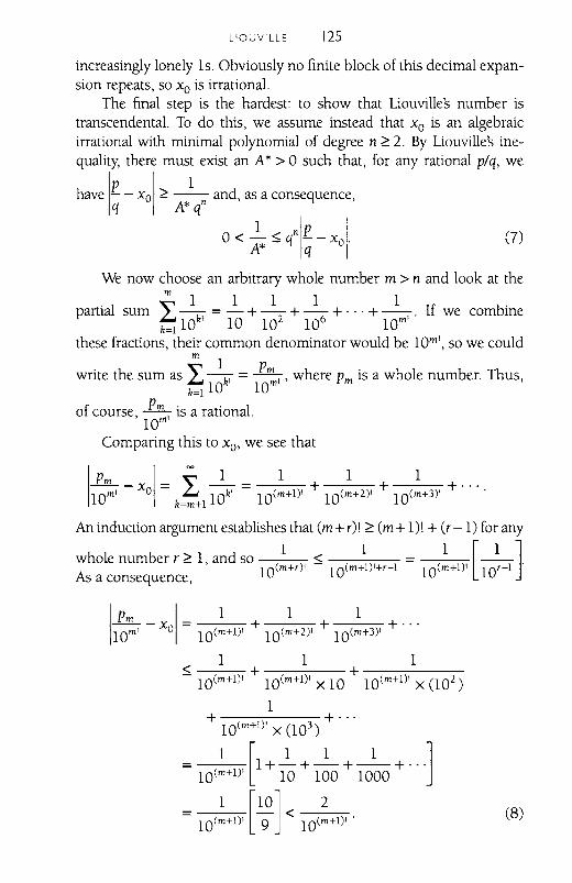
LIOUVILLE 125

increasingly lonely Is. Obviously no finite block of this decimal expan­sion repeats, so Xo is irrational.

The final step is the hardest: to show that Liouville's number istranscendental. To do this, we assume instead that Xo is an algebraicirrational with minimal polynomial of degree n ~ 2. By Liouville's ine­quality, there must exist an A* > 0 such that, for any rational p/q, we

have 1£ - xol ~ _1_ and, as a consequence,

q A' q" 0 <~ ~ q"l£ _xol. (7)A* q

We now choose an arbitrary whole number m > n and look at the

. mIll 1 1 .partIal sum ~ -- = - + -- + - + ... + --. If we combmet lOki 10 102 106 lOm'

these fractions, their common denominator would be 1oml, so we could

m 1write the sum as L -k-I = P':I' where Pm is a whole number. Thus,

k=110 10

of course, Pm I is a rational.10m

Comparing this to xo, we see that

IPm I ~ 1 1 1 1

10m' - X o = £.. lOki = 10(m+I)' + 10(m+2)' + 10(m+3)' + ....k=m+1

An induction argument establishes that (m + r)! ~ (m + I)! + (r-l) for any

1 1 1 [1]whole number r ~ 1, and so < = --10(m+r)' - 10(m+I)'+r-1 10(m+I)' 10r- 1 .

As a consequence,

IPm I 1 1 1

10ml - Xo = 10(m+I)' + 10(m+2)' + 10(m+3)' + ...

1 1 1< + +--,----,------- lO(m+I)' lO(m+I)' X 10 lO(m+I)' X (102)

1+ + ...lO(m+I)' X (103)

= 1O(:+I)' [1 + 1~ + 1~0 + 1O~0 + .. -]

= 10(:+1)1 [ 1~ ] < 1O(:+I)' . (8)

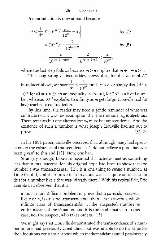
126 CHAPTER 8

A contradiction is now at hand because

by (7)

by (8)

2 2---,---.,... < --10m'(m+l-n) 10m' '10(m+1)'-n(m')

o<~ ~ (lOm'tl~-x IA* 10m' 0

( ml)n 2< 10 . ( 1)110 m+

2

where the last step follows because m > n implies that m + 1 - n > 1.This long string of inequalities shows that, for the value of A*

1 2introduced above, we have - < --I for all m > n, or Simply that 2A* >

A* 10m

lOm' for all m > n. Such an inequality is absurd, for 2A* is a fixed num­ber, whereas lOm' explodes to infinity as m gets large. Liouville had (atlast) reached a contradiction.

By this time, the reader may need a gentle reminder of what wascontradicted. It was the assumption that the irrational Xo is algebraic.There remains but one alternative: Xo must be transcendental. And theexistence of such a number is what Joseph Liouville had set out toprove. Q.E.D.

In his 1851 paper, Liouville observed that, although many had specu­lated on the existence of transcendentals, "I do not believe a proof has everbeen given" to this end [11]. Now, one had.

Strangely enough, Liouville regarded this achievement as somethingless than a total success, for his original hope had been to show that thenumber e was transcendental [12]. It is one thing to create a number, asLiouville did, and then prove its transcendence. It is quite another to dothis for a number like e that was "already there." With his typical flair, EricTemple Bell observed that it is

a much more difficult problem to prove that a particular suspect,like e or Jr, is or is not transcendental than it is to invent a wholeinfinite class of transcendentals: ... the suspected number isentire master of the situation, and it is the mathematician in thiscase, not the suspect, who takes orders. [13]

We might say that Liouville demonstrated the transcendence of a num­ber no one had previously cared about but was unable to do the same forthe ubiquitous constant e, about which mathematicians cared passionately

LIOUVILLE 127

Still, it would be absurd to label him a failure when he found something hispredecessors had been seeking in vain for a hundred years.

That original objective would soon be realized by one of his followers. In1873, Charles Hermite (1822-1901) showed that e was indeed a transcen­dental number. Nine years later Ferdinand Lindemann (1852-1939) provedthe same about Te. As is well known, the latter established the impossibility ofsquaring the circle with compass and straightedge, a problem WIth origins inclassical Greece that had gone unresolved not just for decades or centuriesbut for millennia [141. The results of Hermite and Lindemann were impres­sive pieces of reasoning that built upon Liouvilles pioneering research.

To this day, determining whether a given number is transcendentalranks among the most difficult challenges in mathematics. Much work hasbeen done on this front and many important theorems have been proved,but there remain vast holes in our understanding. Among the great achieve­ments, we should mention the 1934 proof of A. O. Gelfond (1906-1968),which demonstrated the transcendence of an entire family of numbers atonce. He proved that if a is an algebraic number other than 0 or 1 and if bis an irrational algebraic, then ab must be transcendental. This deep result

guarantees, for instance, that 2.fi or (-/2 + VS).J7 are transcendental.Among other candidates now known to be transcendental are eTC, In(2),and sin(1).

However, as of this writing, the nature of such "simple" numbers asTee, ee, and Te TC is yet to be established. Worse, although mathematiciansbelieve in their bones that both Te + e and Te x e are transcendental, no onehas actually proved this [lSI. We repeat: demonstrating transcendence isvery, very hard.

Returning to the subject at hand, we see how far mathematicians hadcome by the mid-nineteenth century. Liouvilles technical abilities inmanipulating inequalities as well as his broader vision of how to attack sodifficult a problem are impressive indeed. Analysis was coming of age.

Yet this proof will serve as a dramatic counterpoint to our main theo­rem from chapter 11. There, we shall see how Georg Cantor found aremarkable shortcut to reach Liouville's conclusion with a fraction of thework. In doing so, he changed the direction of mathematical analysis. TheLiouville-Cantor interplay will serve as a powerful reminder of the con­tinuing vitality of mathematics.

For now, Cantor must wait a bit. Our next object is the ultimate innineteenth century rigor: the mathematics of Karl Weierstrass and thegreatest analytic counterexample of all.

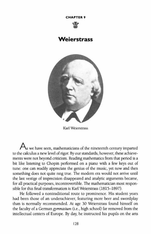
CHAPTER 9

Weierstrass

Karl Weierstrass

As we have seen, mathematicians of the nineteenth century impanedto the calculus a new level of rigor. By our standards, however, these achieve­ments were not beyond criticism. Reading mathematics from that period is abit like listening to Chopin perfonned on a piano with a few keys out oftune: one can readily appreciate the genius of the music, yet now and thensomething does not quite nng true. The modem era would not arrive untilthe last vestige of imprecision disappeared and analytic arguments became,for all practical purposes, incontrovenible. The mathematician most respon­sible for this final transfonnation is Karl Weierstrass (1815-1897).

He followed a nontraditional roule to prominence. His student yearshad been those of an underachiever, featuring more beer and swordplaythan is nonnally recommended. At age 30 Weierstrass found himself onthe faculty of a Gennan gymnasium (Le., high school) far removed from (heintellectual centers of Europe. By day, he instructed his pupils on (he arts

128

WEIERSTRASS 129

of anthmetic and calligraphy, and only after classes were finished and thelessons corrected could young Weierstrass turn to his research [1].

In 1854 this unknown teacher from an unknown town published amemoir on Abelian integrals that astonished the mathematicians who readit. It was evident that the author, whoever he was, possessed an extraordi­nary talent. Within two years, Weierstrass had secured a position at theUniversity of Berlin and found himself on one of the world's great mathe­matics faculties. His was a true Cinderella story.

Weierstrass:S contributions to analysis were as profound as his peda­gogical skills were legendary. With a reputation that spread through Ger­many and beyond, he attracted young mathematicians who wished to learnfrom the master. A school of disciples formed at his feet. This was almostliterally true, for severe vertigo required Weierstrass to lecture from an easychair while a designated student wrote his words upon the board (anarrangement subsequent professors have envied but seldom replicated).

If his teaching style was unusual, so was his attitude toward publica­tion. Although his classes were filled with new and important ideas, heoften let others disseminate such information in their own writings. Thusone finds his results attnbuted somewhat loosely to the School of Weier­strass. Modern academics, operating in "publish or perish" mode, find itdifficult to fathom such a nonpossessive view of scholarship. But Weier­strass acted as though creating significant mathematics was his job, and hewould risk the penshing.

Whether through his own publications or those of his lieutenants, theWeierstrassian school imparted to analysis an unparalleled logical preci­sion. He repaired subtle misconceptions, proved important theorems, andconstructed a counterexample that left mathematicians shaking theirheads. In this chapter, we shall see why Karl Weierstrass came to beknown, in the parlance of the times, as the "father of modern analysis" [2].

BACK TO THE BASICS

We recall that Cauchy built his calculus upon limits, which he definedin these words:

When the values successively attributed to a variable approachindefinitely to a fixed value, in a manner so as to end by differingfrom it by as little as one wishes, this last is called the limit of allthe others.

130 CHAPTER 9

To us, aspects of this statement, for instance, the motion implied in theterm "approach," seem less than satisfactory. Is something actually mov­ing? If so, must we consider concepts of time and space before talking oflimits? And what does it mean for the process to "end"? The whole busi­ness needed one last revision.

Contrast Cauchy's words with the polished definition from the Weier­strassians:

liml(x) = L if and only if, for every £ > 0, there exists a 0 > 0x~

so that, if 0 < Ix - al < 0, then Ij(x) - LI < £. (1)

Here nothing is in motion, and time is irrelevant. This is a static ratherthan dynamic definition and an arithmetic rather than a geometric one. Atits core, it is nothing but a statement about inequalities. And it can beused as the foundation for unambiguous proofs of limit theorems, forexample, that the limit of a sum is the sum of the limits. Such theoremscould now be demonstrated with all the rigor of a proposition from Euclid.

Some may argue that precision comes at a cost, for Weierstrasss austeredefinition lacks the charm of intuition and the immediacy of geometry Tobe sure, a statement like (1) takes some getting used to. But geometricalintuition was becoming suspect, and this purely analytic definition was inno way entangled with space or time.

Besides reformulating key concepts, Weierstrass grasped their mean­ings as his predecessors had not. An example is uniform continuity, aproperty that Cauchy missed entirely. We recall that Cauchy defined con­tinuity on a point-by-point basis, saying that j is continuous at a iflim j(x) = j(a). In Weierstrassian language, this means that to every £ > 0,X~

there corresponds a 0> 0 so that, if 0 < Ix - al < 0, then Ij(x) - j(a)1 < £.

Thus, for a fixed "target" £ and a given a, we can find the necessary o. Buthere 0 depends on both £ and a. Were we to keep the same £ but consider adifferent value of a, the choice of 0 would, in general, have to be adjusted.

It was Eduard Heine (1821-1881) who first drew this distinction inprint, although he suggested that "the general idea" was conveyed to himby his mentor, Weierstrass [3]. Heine defined a function j to be uniformlycontinuous on its domain if, for every £ > 0, there exists a 0> 0 so that, if xand yare any two points in the domain within 0 units of one another, thenIj(x) - j(y)1 < £. This means, in essence, that "one 0 fits all," so that pointswithin this uniform distance will have functional values within £ of oneanother.

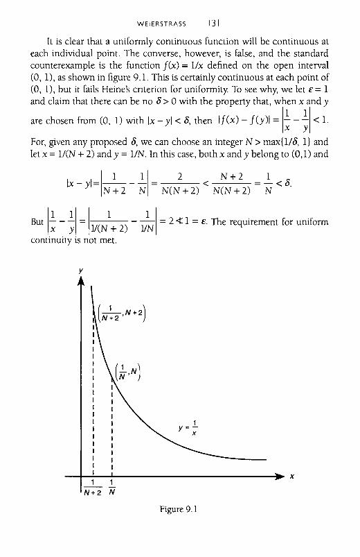
WEIERSTRASS 131

It is clear that a uniformly continuous function will be continuous ateach individual point. The converse, however, is false, and the standardcounterexample is the function j(x) = l/x defined on the open interval(0, 1), as shown in figure 9.1. This is certainly continuous at each point of(0, 1), but it fails Heines cnterion for uniformity To see why, we let E =1and claim that there can be no D> 0 with the property that, when x and y

are chosen from (0, 1) with Ix - yl < D, then Ij(x) - f(y)1 = I~-~I < 1.

For, given any proposed D, we can choose an integer N > max{l/D, l} andlet x = I/(N + 2) and y = liN. In this case, both x and y belong to (0,1) and

1

1 11 2 N+2 1Ix - yl= N + 2 - N = N(N + 2) < N(N + 2) = N < D.

But I~-~I =1 1 - _1_1 = 2 <t:: 1= E. The requirement for uniformx y lI(N + 2) liN

continuity is not met.

y

1y=­x

( _1,N+2)I N+2III11I111111I1IIII11

_-+-....:..1_ ......... • x1 1

N+2 N

Figure 9.1

132 CHAPTER 9

A look back to chapter 6 reminds us that Cauchy had talked aboutcontinuous functions but actually used uniform continuity in some of hisproofs. Fortunately, a logical catastrophe was averted in 1872 whenHeine proved that a function continuous on a closed, bounded interval[a, b] must in fact be uniformly continuous. That is, the distinctionbetween continuity and uniform continuity disappears if we restrict ourattention to [a, b]. (Note that the example above is defined on an openinterval.) So, when Cauchy's misconception occurred for functions onclosed, bounded intervals, his proofs were "salvageable" thanks to Heine'sresult.

Weierstrass recognized an even more crucial dichotomy: that betweenpointWIse and uniform convergence. These ideas warrant a bnef digression.

Suppose we have a sequence of functions, fl, f2, f3, ... , f., ... , allwith the same domain. If we fix a point x in this domain and substitute itinto each function, we generate a sequence of numbers: fl (x), f2(X),f3(X), ... , f.(x), .... Assume that, for each indiVldual x, this numericalsequence converges. We then create a new functionf defined at each pointx by f(x) = lim f. (x). We call f the "pointwise limit" of the f•..~OO

For instance, consider the following sequence of functions on [0, n]:fl (x) = sin x, f2 (x) = (sin X)2, f3 (x) = (sin X)3, ... , f.(x) = (sin x)·, ... ,the first three of which are graphed in figure 9.2.

Weseethat,forallk~ l,f.(~)=(sin~r = 1, and so ~~f{~)=

lim 1 = 1. On the other hand, ifx is in [0, n] but x 7; !!.- , then sin x = r, where.~OO 2

o~ r < 1, and so lim f. (x) = lim (r·) = O. Hence the pointwise limit is.~OO .~OO

f(x) = lim f.(x) = {~.~OO 0

if 0 ~ x < n/2,if x = n/2,ifn/2<x~n,

whose graph is shown in figure 9.3.This example raises one of the great questions of analysis: if each of

the f. has a certain property and f is their pointwise limit, must f itself havethis property? In mathematical parlance, we ask whether a characteristic isinherited by pointWIse limits. If each f. is continuous, must f be continu­ous? If each is integrable, mustfbe integrable?

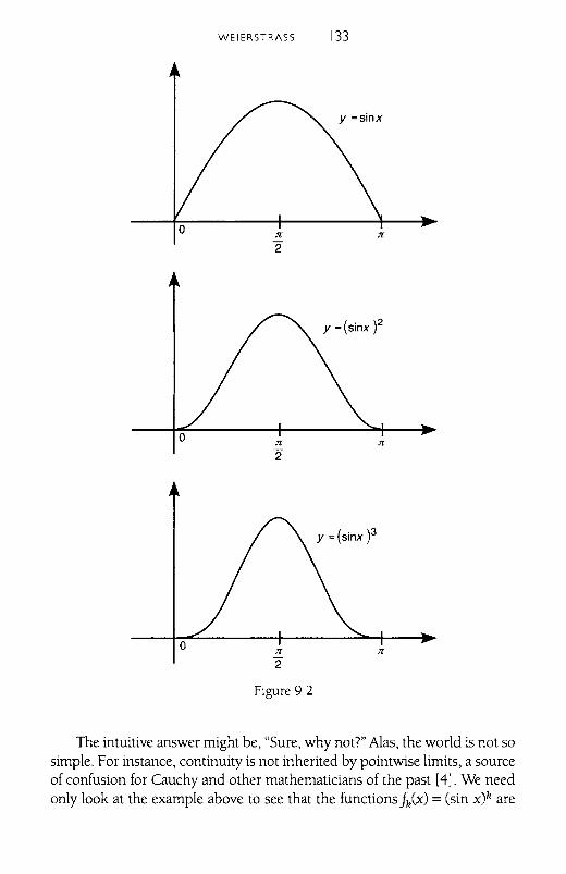
WEIERSTRASS 133

o2

Figure 9 2

The intuitive answer might be, "Sure, why not?" Alas, the world is not sosimple. For instance, continuity is not inherited by pointwise limits, a sourceof confusion for Cauchy and other mathematicians of the past [4]. We needonly look at the example above to see that the functions fh(x) =(sin x)h are

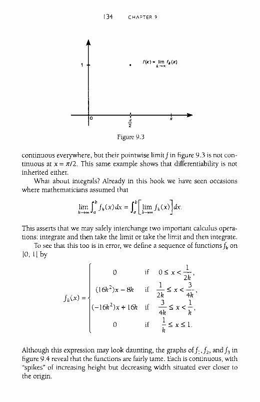
134 CHAPTER 9

I(x) - lim 'k(x)k-oo

o T(

"2

Figure 9.3

continuous everywhere, but their pointwise limitI in figure 9.3 is not con­tinuous at x = Te/2. This same example shows that differentiability is notinherited either.

What about integrals? Already in this book we have seen occasionswhere mathematicians assumed that

This asserts that we may safely interchange two important calculus opera­tions: integrate and then take the limit or take the limit and then integrate.

To see that this too is in error, we define a sequence of functions Ik on[0, I] by

if1

0 o::;x<-2k'

06k 2)x - 8k if1 3-::;x<-

Ik(x) = 2k 4k'3 1

(-I6k 2)x + 16k if -::;x<-4k k'

if1

0 -::; x::; 1.k

Although this expression may look daunting, the graphs ofII ,f2' and 13 infigure 9.4 reveal that the functions are fairly tame. Each is continuous, with"spikes" of increasing height but decreasing width situated ever closer tothe origin.

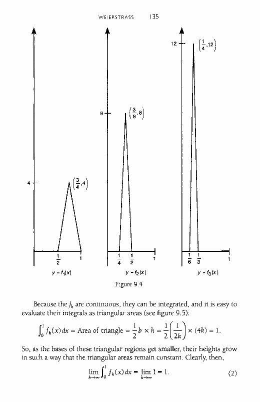
WEIERSTRASS 135

12 (~,12)

8 (~,8)

4

1 1

4 2

Y - '2(x)

Figure 9.4

1 16 3

Y - '3 (x)

Because the fh are continuous, they can be integrated, and it is easy toevaluate their integrals as triangular areas (see figure 9.5):

11 1 1 ( 1 )fh(x)dx = Area of triangle = -b x h = - - x (4k) = 1.o 2 2 2k

So, as the bases of these triangular regions get smaller, their heights growin such a way that the triangular areas remain constant. Clearly, then,

lim rIfh(x)dx = lim 1= 1. (2)

h~~JO k~~

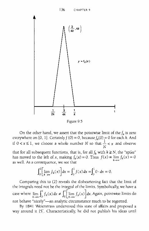
136 CHAPTER 9

1 3 12k 4k k

Figure 9.5

On the other hand, we assert that the pointwise limit of the fk is zeroeverywhere on [0, 1]. Certainly f (0) = 0, because fk(O) = 0 for each k. And

if 0 < x:::; 1, we choose a whole number N so that ~ < x and observeN

that for all subsequent functions, that is, for all fk with k ~ N, the "spike"has moved to the left of x, making fk(x) =O. Thus f(x) = lim fk(x) = 0

k~oo

as well. As a consequence, we see that

r1[lim fk(X)]dx = r1f(x)dx =rIo· dx = o.Jo k~oo Jo Jo

Comparing this to (2) reveals the disheartening fact that the limit ofthe integrals need not be the integral of the limits. Symbolically, we have a

case where lim r1

fk(X)dx 7; r1[lim fk (X)] dx. Again, pointwise limits dok~oo 10 Jo k~oo

not behave "nicely"-an analytic circumstance much to be regretted.By 1841 Weierstrass understood this state of affairs and proposed a

way around it [5]. Characteristically, he did not publish his ideas until

WEIERSTRASS 137

1894-more than half a century later-but his students had spread theword long before. The idea was to introduce a stronger form of conver­gence, called uniform convergence, under which key properties transferfrom indiVIdual functions to their limit.

Following his lead, we define a sequence of functions fn to convergeuniformly to a functionf on a common domain if for every e> 0, there isa whole number N so that, if k ~ N and if x is any point in the domain,then Ifn(x) - f(x) I < e. In a manner reminiscent of uniform continuity, thissays that "one N fits all x" in the domain of the functions fn.

This mode of convergence can be illustrated geometrically. Givene> 0, we draw a band of WIdth e surrounding the graph of y =f(x), asshown in figure 9.6. By uniform convergence, we must reach a subscriptN so that fN and all subsequent functions in the sequence lie entirely WIth­in this band. As the name suggests, such functions approximate f uni­formly across the interval [a, b].

It is easy to see that if a sequence of functions converges uniformly to1, then it converges pointWIse to 1, but not conversely. For example, the"spike" functions described above converge pointwise but not uniformlyto the zero function on [0, 1]. Uniform convergence is a stronger, morerestrictive phenomenon than mere pointWIse convergence.

We have undertaken this digression for a few reasons. First, we shallneed the notion of uniform convergence in the chapters main result. Sec­ond, echoes of these ideas appear throughout the remainder of the book.Finally, such considerations illustrate why Weierstrass is so important inthe history of calculus. In the words of Victor Katz,

Not only did Weierstrass make absolutely clear how certain quan­tities in his definition(s) depended on other quantities, but he alsocompleted the transformation away from the use of terms such as"infinitely small." Henceforth, all definitions involving such ideaswere given arithmetically [6].

FOUR GREAT THEOREMS

Besides revisiting definitions, Weierstrass was a master at emplOYIngthem to prove theorems of importance. Here we shall mention (but notprove) four of his results involving uniform convergence.

The first two address a topic mentioned above: under uniform con­vergence, important analytic properties transfer from the individual fn tothe limit function f

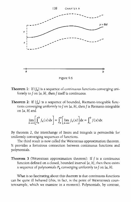
r---I

Ii II

a

138 CHAPTER 9

-------- ......................................

--------,

Figure 9.6

­,----,,"

y=f(x)

...... _---,,;

b

Theorem 1: If Uk} is a sequence of continuous functions converging uni­formly to f on la, b], then f itself is continuous.

Theorem 2: If Uk} is a sequence of bounded, Riemann-integrable func­tions converging uniformly to f on la, b], then f is Riemann-integrableon la, b] and

lim [f fk(X)dx] = Jb[lim fk(X)]dx = Jb f(x)dx.k~oo a a k~oo a

By theorem 2, the interchange of limits and integrals is permissible foruniformly converging sequences of functions.

The third result is now called the Weierstrass approximation theorem.It provides a fortuitous connection between continuous functions andpolynomials.

Theorem 3 (Weierstrass approximation theorem): If f is a continuousfunction defined on a closed, bounded interval [a, b], then there existsa sequence of polynomials Pk converging uniformly to f on la, b].

What is so fascinating about this theorem is that continuous functionscan be quite ill behaved (this, in fact, is the point of Weierstrasss coun­terexample, which we examine in a moment). Polynomials, by contrast,

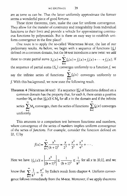
WEIERSTRASS 139

are as tame as can be. That the latter uniformly approximate the formerseems a wonderful piece of good fortune.

These three theorems, then, make the case for uniform convergence.They allow for the transfer of continuity and integrability from indiVIdualfunctions to their limit and provide a vehicle for approximating continu­ous functions by polynomials. But is there an easy way to establish uni­form convergence in the first place?

One route is to apply the so-called Weierstrass M-test, the last of ourpreliminary results. As before, we begin with a sequence of functions 11k Idefined on a common domain, but the M-test introduces a new twist: we add

n

these to create partial sums Sn(x) = IJh(X) = fr(x)+ f2(X)+' .. + fn(x). Ifh=l

the sequence of partial sums ISn I converges uniformly to a function f, we

say the infinite series of functions Lfh(X) converges uniformly toh=l

f With this background, we now state the follOwing result.

Theorem 4 (Weierstrass M-test): If a sequence {[hI of functions defined on acommon domain has the property that, for each k, there exists a positivenumber Mhso that Ifh(X) I~ Mh for all x in the domain and if the infinite

~

series LMhconverges, then the series offunctions L!k(x) convergesh~ h~

uniformly.

This amounts to a comparison test between functions and numbers,where convergence of the series of numbers implies uniform convergenceof the series of functions. For example, consider the function defined on[0, I] by

Here we have Ifh(x)1 = xh

~ 1 ~ ~ for all x in [0,11, and we(k + 1)3 (k + I? k2

~ 2

know that L~ = !!.- by Euler's result from chapter 4. Uniform conver-h=l k2 6

gence follows immediately from the M-test. Moreover, if we apply theorems

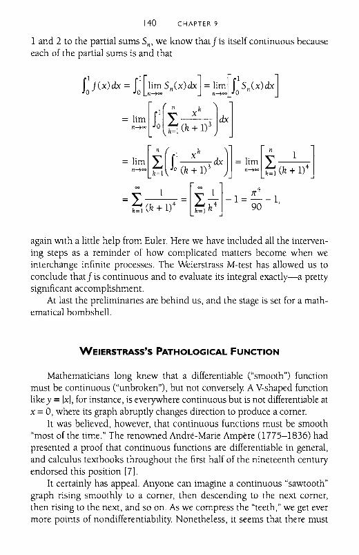
140 CHAPTER 9

1 and 2 to the partial sums Sn, we know that j is itself continuous becauseeach of the partial sums is and that

rlj(x)dx = rl[lim Sn(x)dx] =lim[r

lSn(X)dx]Jo Jo n~~ n~~ Jo

[ [n k J ]I X

= lim dxn~~ fo ~ (k + 1)3

[n (I x

k)] [ n 1 ]- lim dx - lim

- n~~ ~ fa (k + 1)3 - n~~ ~ (k + 1)4

~ 1 [~1 ] 7(4- - - -1---1-~(k+1)4 - ~k4 -90 '

again WIth a little help from Euler. Here we have included all the interven­ing steps as a reminder of how complicated matters become when weinterchange infinite processes. The Weierstrass M-test has allowed us toconclude that j is continuous and to evaluate its integral exactly-a prettysignificant accomplishment.

At last the preliminanes are behind us, and the stage is set for a math­ematical bombshell.

WEIERSTRASS'S PATHOLOGICAL FUNCTION

Mathematicians long knew that a differentiable ("smooth") functionmust be continuous ("unbroken"), but not conversely A V-shaped functionlike y = lxi, for instance, is everywhere continuous but is not differentiable atx =0, where its graph abruptly changes direction to produce a corner.

It was believed, however, that continuous functions must be smooth"most of the time." The renowned Andre-Marie Ampere (1775-1836) hadpresented a proof that continuous functions are differentiable in general,and calculus textbooks throughout the first half of the nineteenth centuryendorsed this position [7].

It certainly has appeal. Anyone can imagine a continuous "sawtooth"graph rising smoothly to a corner, then descending to the next corner,then rising to the next, and so on. As we compress the "teeth," we get evermore points of nondifferentiability Nonetheless, it seems that there must

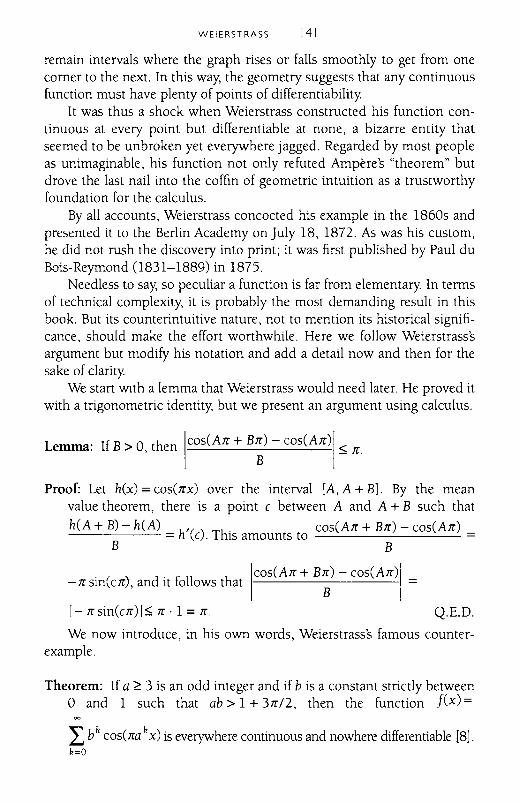
WEIERSTRASS 141

remain intervals where the graph rises or falls smoothly to get from onecorner to the next. In this way, the geometry suggests that any continuousfunction must have plenty of points of differentiability.

It was thus a shock when Weierstrass constructed his function con­tinuous at every point but differentiable at none, a bizarre entity thatseemed to be unbroken yet everywhere jagged. Regarded by most peopleas unimaginable, his function not only refuted Ampere's "theorem" butdrove the last nail into the coffin of geometric intuition as a trustworthyfoundation for the calculus.

By all accounts, Weierstrass concocted his example in the 1860s andpresented it to the Berlin Academy on July 18, 1872. As was his custom,he did not rush the discovery into print; it was first published by Paul duBois-Reymond (1831-1889) in 1875.

Needless to say, so peculiar a function is far from elementary. In termsof technical complexity, it is probably the most demanding result in thisbook. But its counterintuitive nature, not to mention its historical signifi­cance, should make the effort worthwhile. Here we follow Weierstrass'sargument but modify his notation and add a detail now and then for thesake of clarity.

We start Wlth a lemma that Weierstrass would need later. He proved itwith a trigonometric identity, but we present an argument using calculus.

Lemma: If B> 0, then ICOS(AJr + B~) - COS(AJr)! ~ Jr.

Proof: Let hex) =cos(Jrx) over the interval [A, A + B]. By the meanvalue theorem, there is a point c between A and A + B such that

h(A + B) - h(A) h'() Th' cos(AJr + BJr) - cos(AJr)= C. IS amounts to =B B

ICOS(AJr + BJr) - COS(AJr)1

- Jr sin(c Jr), and it follows that B =

1- Jrsin(cJr)I~ Jr. 1 =Jr. Q.E.D.

We now introduce, in his own words, Weierstrass's famous counter-example.

Theorem: If a ~ 3 is an odd integer and if b is a constant strictly between° and 1 such that ab> 1 + 3Jr/2, then the function j(x)=

L bkcos(Jra kx) is everywhere continuous and nowhere differentiable [8].

k=O

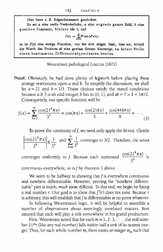
142 CHAPTER 9

Dies kann z. B. folgendermassen geschehen.Es sei x eine reelle Veriinderliche, a eine ungrade ganze Zahl, b eine

positive Constante, kleiner als 1, und

(x) = i; b" cos (a" x,,) i"=0

so ist ((x) eine stetige Function, von der sich zeigen liisst, dass sie, sobaldder Werth des Products ab eine gewisse Grenze iibersteigt, an keiner Stelleeinen bestimmten Differentialquotienten besitzt.

Weierstrasss pathological function (872)

Proof: Obviously, he had done plenty of legwork before placing thesestrange restrictions upon a and b. To simplify the discussion, we shalllet a = 2l and b = 1/3. These choices satisfy the stated conditionsbecause a ~ 3 is an odd integer, b lies in (0, 1), and ab =7 > 1 + 3Jr/2.Consequently, our specific function will be

~ h

J()~ cos(2l Jrx) () cos(2lJrx) cos(441Jrx)

x = £... k = cos Jr X + + + ....h=O 3 3 9 (3)

To prove the continuity off, we need only apply the M-test. Clearlyh ~

cos(2l Jrx) <~ and L~ converges to 3/2. Therefore, the senes3k - 3k 3h

h=O

cos(2l hJrx)converges uniformly to j. Because each summand is

3h

continuous everywhere, so isJby theorem 1 above.

We seem to be halfway to showing thatJis everywhere continuousand nowhere differentiable. However, proving the "nowhere differen­tiable" part is much, much more difficult. To this end, we begin by fixinga real number r. Our goal is to show that r(r) does not exist. Because ris arbitrary, this will establish thatJis differentiable at no point whatever.

In following Weierstrasss logic, it will be helpful to assemble anumber of observations about seemingly unrelated matters. Restassured that each will playa role somewhere in his grand production.

First, Weierstrass noted that for each m =1, 2, 3, ... , the real num­ber 21 mr (like any real number) falls within half a unit of its nearest inte­ger. Thus, for each whole number m, there exists an integer am such that

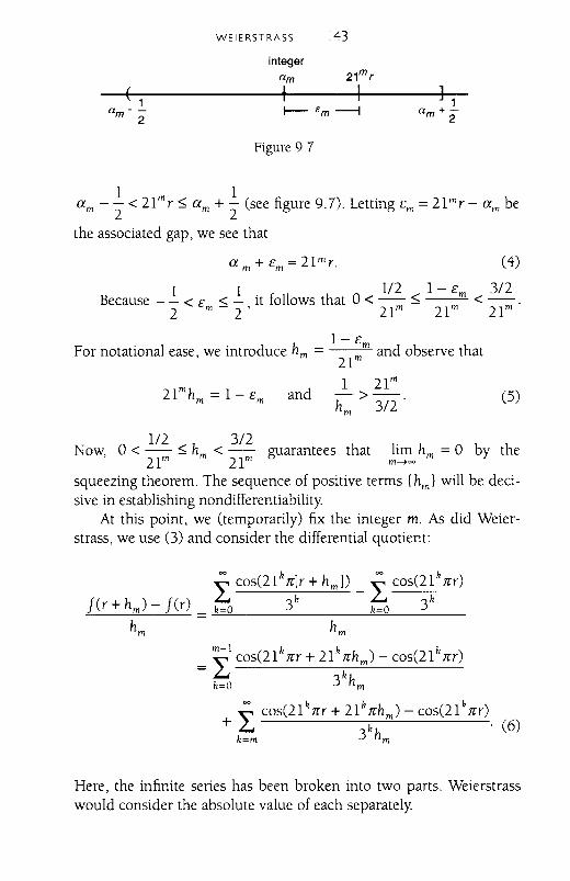
( 1a -­

m 2

WEIERSTRASS 143

integeram 21 m ,

f II-- cm---f

Figure 9 7

am _l < 21 m r $ am + l (see figure 9.7). Letting Em =21 mr- am be2 2

the associated gap, we see that

(4)

1 1 1/2 1 - Em 3/2Because - - < E < - it follows that 0 < -- $ -- < --.

2 m - 2 ' 21 m 21 m 21 m

l-EFor notational ease, we introduce hm =~ and observe that

21

and1 21m

->--.hm 3/2

(5)

1/2 3/2Now, 0 < -- $ hm < -- guarantees that lim hm = 0 by the

21 m 21mm--t=

squeezing theorem. The sequence of positive terms {hml will be deci­sive in establishing nondifferentiability

At this point, we (temporarily) fix the integer m. As did Weier­strass, we use (3) and consider the differential quotient:

Here, the infinite series has been broken into two parts. Weierstrasswould consider the absolute value of each separately

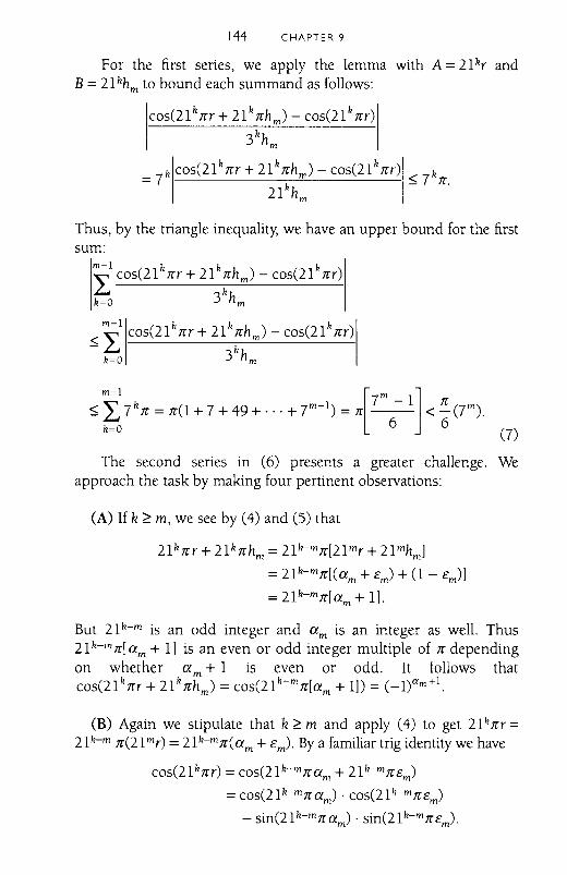
144 CHAPTER 9

For the first series, we apply the lemma with A =21 kr andB =21 khm to bound each summand as follows:

cos(ll knr + II knh m) - cos(ll knr)

3khm

7k cos(ll knr + II knhm) - cos(ll knr) k

= k ~ 7 n.II hm

Thus, by the triangle inequality, we have an upper bound for the firstsum:

m-I k k kL cos(ll nr + II nhm) - cos(ll nr)

k=O 3khm

m-I k k k~ L cos(ll nr + II ~hm) - cos(ll nr)

k=O 3 hm

m-I [7 m_ 1] n

~ L t kn = n(1 + 7 + 49 + ... + 7m-

l) = n -- < -(r).

k=O 6 6 (7)

The second series in (6) presents a greater challenge. Weapproach the task by making four pertinent observations:

(A) If k ~ m, we see by (4) and (5) that

IIknr + II knhm= llk-mn[ll mr + II mhm]

=IIk-mn[(am+ Em) + (1- Em)]

= II k-m n[ am + 1].

But llk-m is an odd integer and am is an integer as well. Thus21 k-m n[ am + 1] is an even or odd integer multiple of n dependingon whether am + 1 is even or odd. It follows thatcos(llk nr + llknh m) = cos(llk-mn[am + 1]) = (_l)Um+l.

(B) Again we stipulate that k ~ m and apply (4) to get II knr =IIk-m n(llmr) =IIk-mn(am + Em)' Bya familiar trig identity we have

cos(llknr) =cos(ll k-mnam+ IIk-mn Em)

=COs(llk-mnam) . cos(ll k-m mom )

- sin(21 k-m n am) . sin(21 k-m n Em)'

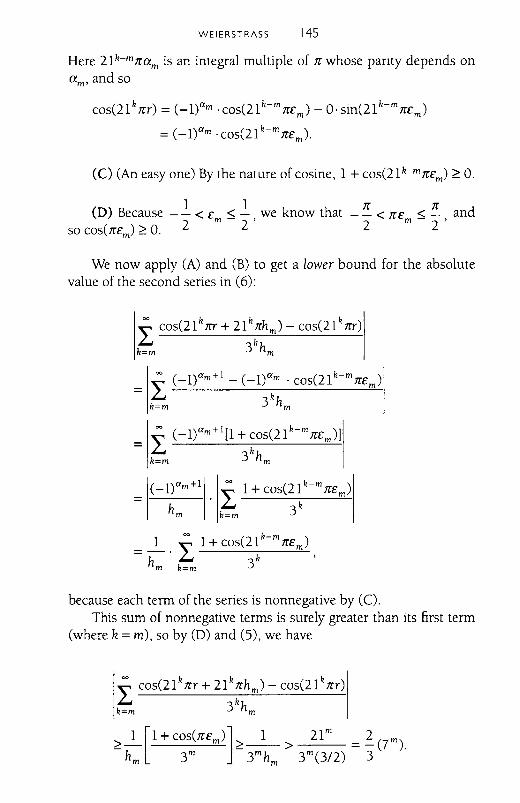
WEIERSTRASS 145

Here 21 h-mJram is an integral multiple of Jr whose panty depends onam' and so

cos(21 hJrr) = (_l)am.cos(21 h-m JrEm

) - O· sin(21 h-m JrEm )

= (_l)am ·cos(21h-mJrEm)·

(C) (An easy one) By the nature of cosine, 1 + cos(21h-mJrEm) ~ O.

1 1 Jr Jr(D) Because - - < E < - we know that - - < JrE ~ - and

so COS(JrEm

) ~ O. 2 m - 2 ' 2 m 2'

We now apply (A) and (B) to get a lower bound for the absolutevalue of the second series in (6):

i: cos(21 hnr + 21 hJrh m ) - cos(21 hnr)

h=m 3h

h m

= i: (_l)am +l - (_l)am . cos(21h-mJrEm )

h=m 3h

h m

= i: (_l)am +1 [1 + cos(21 k-m JrEm )I

k=m 3k

h m

i: 1+ cos(2 ~k-m JrEm )

k=m 3

because each term of the series is nonnegative by (C).This sum of nonnegative terms is surely greater than its first term

(where k =m), so by (D) and (5), we have

i: cos(21 k Jrr + 21 k Jrh m ) - cos(21 k Jrr)

k=m 3k

h m

~_1 [l+COS(JrEm)]~_l_ > 21m

= ~(7m).h m 3m 3m

h m 3m (3/2) 3

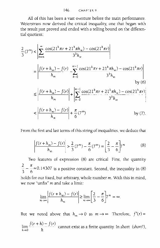
146 CHAPTER 9

All of this has been a vast overture before the main performance.Weierstrass now derived the critical inequality, one that began withthe result Just proved and ended with a telling bound on the differen­tial quotient:

= fCr+h m )- fCr) _IIcosC2lkll'r+2lkll'hm)-cosC2lkll'r)

hm k=O 3khm

by (6)

~ Ifcr + h;) -fCr)1 + I cosC2l k ll'r + 2l k:hm ) - cosC2l k ll'r)

m k=O 3 hm

by (7).

From the first and last terms of this string of inequalities, we deduce that

Two features of expression (8) are critical First, the quantity2 ll'"3 - (5 Z 0.14307 is a positive constant. Second, the inequality in (8)

holds for our fixed, but arbitrary, whole number m. With this in mind,we now "unfix" m and take a limit:

But we noted above that hm ~ 0 as m ~ 00 Therefore, j'Cr) =

1. fCr + h) - fCr)1m cannot exist as a finite quantity. In short Cshort?),

h-tO h

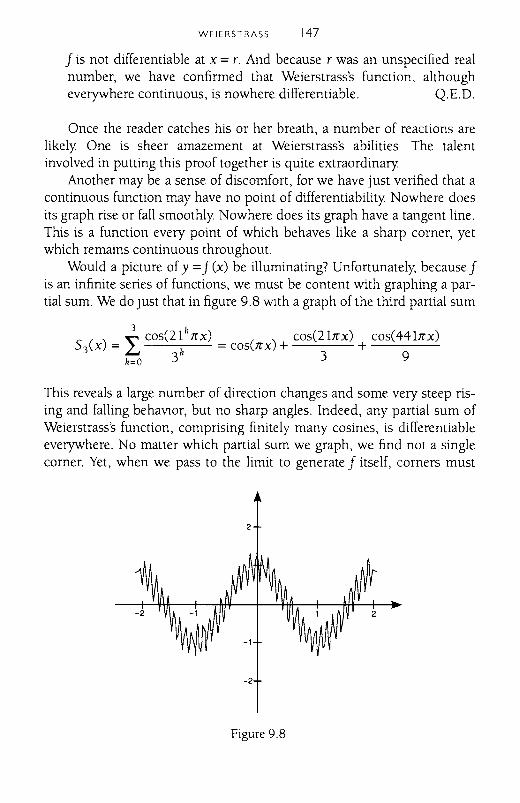
WEIERSTRASS 147

J is not differentiable at x = r. And because r was an unspecified realnumber, we have confirmed that Weierstrass's function, althougheverywhere continuous, is nowhere differentiable. Q.E.D.

Once the reader catches his or her breath, a number of reactions arelikely One is sheer amazement at Weierstrass's abilities The talentinvolved in putting this proof together is quite extraordinary.

Another may be a sense of discomfort, for we have just verified that acontinuous function may have no point of differentiability Nowhere doesits graph rise or fall smoothly Nowhere does its graph have a tangent line.This is a function every point of which behaves like a sharp corner, yetwhich remains continuous throughout.

Would a picture of y =J(x) be illuminating? Unfortunately, because Jis an infinite series of functions, we must be content with graphing a par­tial sum. We do Just that in figure 9.8 WIth a graph of the third partial sum

5 ()~ cos(21kJrx) () cos(21Jrx) cos(441Jrx)

3 x = £.J k = cos Jr X + + ---'-------'-k=O 3 3 9

This reveals a large number of direction changes and some very steep ris­ing and falling behavlOr, but no sharp angles. Indeed, any partial sum ofWeierstrass's function, comprising finitely many cosines, is differentiableeverywhere. No matter which partial sum we graph, we find not a singlecorner. Yet, when we pass to the limit to generate J itself, corners must

-2

Figure 9.8

148 CHAPTER 9

appear everywhere. Weierstrass's function lies somewhere beyond the intu­ition, far removed from geometrical diagrams that can be sketched on ablackboard. Yet its existence has been unquestionably established in theproof above.

A final reaction to this argument should be applause for its high stan­dard of rigor. Like a maestro conducting a great orchestra, Weierstrassblended the fundamental definitions, the absolute values, and a host ofinequalities into a coherent whole. Nothing was left to chance, nothing tointuition. For later generations of analysts, the ultimate compliment wasto say that a proof exhibited "Weierstrassian rigor."

To be sure, not everyone was thrilled by a function so pathological.Some critics reacted against a mathematical world where inequalitiestrumped intuition. Charles Hermite, whom we met in the previous chap­ter, famously bemoaned the discovery in these words: "I turn away withfright and horror from this lamentable evil of functions that do not havederivatives" [9]. Henri Poincare (1854-1912) called Weierstrasss example"an outrage against common sense" [10]. And the exasperated Emile Picard(1856-1941) wrote: "If Newton and Leibniz had thought that continuousfunctions do not necessarily have a derivative ... the differential calculuswould never have been invented" [11]. As though cast out of Eden, thesemathematicians believed that paradise-in the form of an intuitive, geo­metric foundation for calculus-had been lost forever.

But Weierstrasss logic was ironclad. Short of abandoning the defini­tions of limit, continuity, and differentiability, or of denying analysts theright to introduce infinite processes, the critics were doomed. If some­thing like a continuous, nowhere-differentiable function was intuitivelytroubling, then scholars needed to modify their intuitions rather thanabandon their mathematics. Analytic rigor, advancing since Cauchy,reached a new pinnacle with Weierstrass. Like it or not, there was no turn­ing back.

In a continuing ebb and flow, mathematicians develop grand theoriesand then find pertinent counterexamples to reveal the boundanes of theirideas. This juxtaposition of theory and counterexample is the logicalengine by which mathematics progresses, for it is only by knowing howproperties fail that we can understand how they work. And it is only byseeing how intuition misleads that we can truly appreciate the power ofreason.

CHAPTER 10

Second Interlude

Our story has reached the year 1873, nearly a century after the pass­ing of Euler and two after the creation of the calculus. By that date, thework of Cauchy, Riemann, and Weierstrass was sufficient to silence anylatter-day Berkeley who might happen along. Was there anything left to do?

The answer, of course, is ... "Of course." As mathematicians grappledwith ideas like continuity and integrability, their very successes raisedadditional questions that were intriguing, troubling, or both. Weierstrass'spathological function was the most famous of many peculiar examplesthat suggested avenues for future research. Here we shall consider a fewothers, each of which Wlll figure in the book's remaining chapters.

Our first is the so-called "ruler function," a Simple but provocativeexample that appeared in a work of Johannes Karl Thomae 0840-1921)from 1875. He introduced it Wlth this preamble: "Examples of integrablefunctions that are continuous or are discontinuous at individual points areplentiful, but it is important to identify integrable functions that are dis­continuous infinitely often" [1].

His function was defined on the open interval (0, 1) by

r( ) = {lIq if x = plq in lowest terms,x 0 if x is irrational.

Thus, r(I/S) = r(2/S) = r(4/l0) = lIS, whereas r(;r/6) = r(lI-,J2) = 0 Figure10.1 displays the portion of its graph above y = 1/7; below this, the scat­tered points become impOSSibly dense. The graph suggests the verticalmarkings on a ruler-hence the name.

With the E-D definition from the previous chapter, it is easy to provethe follOwing lemma.

Lemma: If a is any point in (0, 1), then lim rex) = O.x~a

Proof: For E> 0, we chose a whole number N with lIN < E. The proofrests upon the observation that in (0, 1) there are only finitely many

149

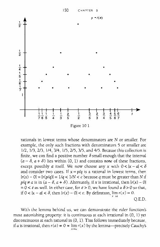
12

150 CHAPTER 10

y =r(x)

•

13 • •

1 •41 • • • •51 • •61 • • • • •"7

111 1 12765 4 3 5

12

3 2 3 4 5 65 3 4 5 6 7

Figure 10 1

rationals in lowest terms whose denominators are N or smaller. Forexample, the only such fractions with denominators 5 or smaller are1/2, 1/3,2/3, 1/4,3/4, 1/5,2/5,3/5, and 4/5. Because this collection isfinite, we can find a positive number 8 small enough that the interval(a - 8, a + 8) lies within (0, 1) and contains none of these fractions,except possibly a itself. We now choose any x with 0 < Ix - al < 8and consider two cases. If x =plq is a rational in lowest terms, thenIr(x) - 01 = Ir(plq) I = l/q < liN < c because q must be greater than N ifplq "* a is in (a - 8, a + 8). Alternately, if x is irrational, then Ir(x) - 01=0 < c as well. In either case, for c> 0, we have found a 8> 0 so that,if 0 < Ix - al < 8, then Ir(x) - 01 < c. By definition, lim rex) = O.

x->aQ.E.D.

With the lemma behind us, we can demonstrate the ruler functionsmost astonishing property: it is continuous at each irrational in (0, 1) yetdiscontinuous at each rational in (0, 1). This follows immediately because,if a is irrational, then rea) = 0 = lim rex) by the lemma-precisely Cauchys

X---7Q

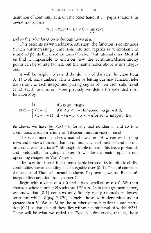
SECOND INTERLUDE [51

definition of continuity at a. On the other hand, if a =p/q is a rational inlowest terms, then

rea) = r(p/q) = l/q 7; °= lim rex),x--->a

and so the ruler function is discontinuous at a.This presents us with a bizarre situation: the function is continuous

(which our increasingly unreliable intuition regards as "unbroken") atirrational points but discontinuous ("broken") at rational ones Most ofus find it impossible to envision how the continuity/discontinuitypoints can be so intertwined. But the mathematics above is unambigu­ous.

It WIll be helpful to extend the domain of the ruler function from(0, 1) to all real numbers. This is done by letting our new function takethe value 1 at each integer and putting copies of r on each subinterval(1,2), (2,3), and so on. More precisely, we define the extended rulerfunction R by

R(x) = {~(x - n)rex + n + 1)

if x is an integer,ifn < x < n + 1for some integern ~ 0,if - (n + 1) < x < - n for some integern ~ 0.

As above, we have lim R(x) = ° for any real number a, and so R isx--->a

continuous at each irrational and discontinuous at each rational.The ruler function raises a natural question: "How can we flip-flop

roles and create a function that is continuous at each rational and discon­tinuous at each irrational?" Although Simple to state, this has a profound,and profoundly intriguing, answer. It will be the main topic in ourupcoming chapter on Vito Volterra.

The ruler function R is also remarkable because, its infinitude of dis­continuities notWIthstanding, it is integrable over [0, 1]. That, of course, isthe essence of Thomae's preamble above. To prove it, we use Riemann'sintegrability condition from chapter 7.

Begin with a value of d > °and a fixed oscillation (J> 0. We thenchoose a whole number N such that l/N < (J. As in the argument above,we know that [0,1] contains only finitely many rationals in lowestterms for which R(p/q) ~ l/N, namely those with denominators nogreater than N. We let M be the number of such rationals and parti­tion [0,1] so that each of these lies within a subinterval of width d/2M.These will be what we called the Type A subintervals, that is, those

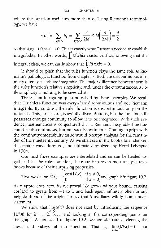
[52 CHAPTER 10

where the function oscillates more than a. Using Riemann's terminol­ogy, we have

d ( d) dsea) = L Ok = L - ~ M - = -,Type A Type A 2M 2M 2

so that s(a) ~ 0 as d~ O. This is exactly what Riemann needed to establish

integrability. In other words, f: R(x)dx exists. Further, knowing that the

integral exists, we can easily show that f~ R(x)dx = o.It should be plain that the ruler function plays the same role as Rie­

mann's pathological function from chapter 7. Both are discontinuous infi­nitely often, yet both are integrable. The major difference between them isthe ruler function's relative Simplicity, and, under the circumstances, a lit­tle Simplicity is nothing to be sneered at.

There is an intriguing question raised by these examples. We recallthat Dirichlet's function was everywhere discontinuous and not Riemannintegrable. By contrast, the ruler function is discontinuous only on therationals. This, to be sure, is awfully discontinuous, but the function stillpossesses enough continuity to allow it to be integrated. With such evi­dence, mathematicians conjectured that a Riemann-integrable functioncould be discontinuous, but not too discontinuous. Coming to grips withthe continuitylintegrability issue would occupy analysts for the remain­der of the nineteenth century. As we shall see in the book's final chapter,this matter was addressed, and ultimately resolved, by Henri Lebesguein 1904.

Our next three examples are interrelated and so can be treated to­gether. Like the ruler function, these are fixtures in most analysis text­books because of their surprising properties.

{COS(l! x) if x*- 0,

First, we define Sex) = 0 if x = 0, and graph it in figure 10.2.

As x approaches zero, its reciprocal 1/x grows without bound, causingcosO/x) to gyrate from -1 to 1 and back again infinitely often in anyneighborhood of the origin. To say that S oscillates wildly is an under­statement.

We show that lim Sex) does not exist by introducing the sequencex-tO

{II/ur} for k = 1, 2, 3, ... and looking at the corresponding points onthe graph. As indicated in figure 10.2, we are alternately selecting the

crests and valleys of our function. That is, lim(l/krr) = 0, butk-t=

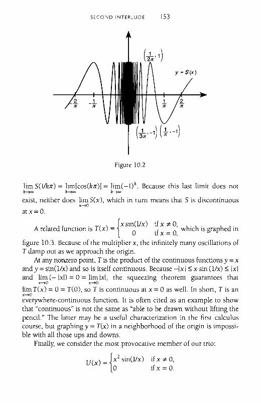
SECOND INTERLUDE 153

Figure 10.2

lim S(lIkn) = lim[cos(kn)] = lim(-l)k. Because this last limit does notk--?oo k--?oo k--?oo

exist, neither does lim Sex), which in turn means that 5 is discontinuousX--?O

atx= O.

{xsin(l!X) if x :I:- 0,

A related function is T(x) = 0 if x = 0, which is graphed in

figure 10.3. Because of the multiplier x, the infinitely many oscillations ofT damp out as we approach the origin.

At any nonzero point, T is the product of the continuous functions y = xand y = sinO/x) and so is itself continuous. Because -Ixl ~ x sin O/x) ~ Ixland lim (- Ixl) = 0 = lim lxi, the squeezing theorem guarantees that

x--?O x--?O

lim T(x) = 0 = T(O), so T is continuous at x = 0 as well. In short, T is anx--?Oeverywhere-continuous function. It is often cited as an example to showthat "continuous" is not the same as "able to be drawn without lifting thepencil." The latter may be a useful characterization in the first calculuscourse, but graphing y = T(x) in a neighborhood of the origin is impossi­ble with all those ups and downs.

Finally, we consider the most provocative member of our trio:

Vex) = {x2

sin(l!x) if x :I:- 0,o if x = O.

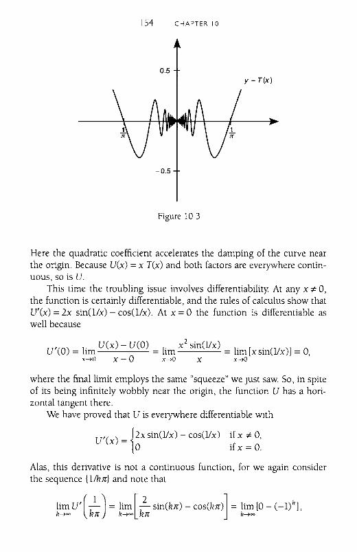
154 CHAPTER 10

0.5y = T(x)

-0.5

Figure 103

Here the quadratic coefficient accelerates the damping of the curve nearthe origin, Because Vex) =x rex) and both factors are everywhere contin­uous, so is V.

This time the troubling issue involves differentiability At any x;t. 0,the function is certainly differentiable, and the rules of calculus show thatV'(x) =2x sinO/x) - cosO/x). At x =0 the function is differentiable aswell because

V '(O) I' Vex) - V(O) I' x2

sin(lIx) I' [ , (11)] 0= 1m = 1m = 1m x SIn x =x~o X - 0 x~o X x~o '

where the final limit employs the same "squeeze" we Just saw. So, in spiteof its being infinitely wobbly near the origin, the function V has a hori­zontal tangent there.

We have proved that V is everywhere differentiable with

V'(x) = {2X sin(llx) - cos(llx) if x ;t. 0,o If x = O.

Alas, this derivative is not a continuous function, for we again considerthe sequence {1//ur} and note that

lim V' (_1)= lim [~sin(kJr) - COS(kJr)] = lim [0 - (_I)h],h~= kJr h~= kJr h~=

SECOND INTERLUDE 155

which does not exist. Thus, lim U'(x) cannot exist and so U' is discontin­X---70

uous at x = O. In short, U is a differentiable function with a discontinuousderivative.

This brings to mind the famous theorem that a differentiable functionis continuous. It would be natural to propose the following modification:"The derivative of a differentiable function must be continuous." Theexample of U, however, shows that such a modification is wrong.

These examples also muddy the relationship between continuity andthe intermediate value theorem. As we saw, Cauchy proved that a continu­ous function must take all values between any two that it assumes. Thisgeometrically self-eVIdent fact might appear to be the very essence of conti­nuity, and one could surmise that a function is continuous if and only if itpossesses the intermediate value property over every interval of its domain.

Again, this assumption turns out to be erroneous. As a counterexample,consider S from above. We have seen that S is discontinuous at the ongin,but we claim that it has the intermediate value property over every interval.

To prove this, suppose Sea) ~ r ~ S(b) for a < b. By the nature of thecosine, we know that -1 ~ r ~ 1. We now consider cases:

If 0 < a < b or if a < b < 0, then S is continuous throughout [a, bl andso, for some c in (a, b), we have S(c) = r by the intermediate value theorem.

On the other hand, if a < 0 < b, we can fix a whole number N with1 1 1

N > -- Then a < 0 < < -- < b, and as x runs between the2Jrb (2N + l)Jr 2NJr

1 1positive numbers ( ) and -2-' the value of l/x runs between 2NJr

2N + 1 Jr NJrand (2N + l)Jr. In the process, Sex) =cosO/x) goes continuously fromcos(2NJr) = 1 to cos[(2N + l)nl = -1. By the intermediate value theorem,

1 1there must be a c between and -- (and consequently between

(2N + l)Jr 2NJra and b) for which S(c) = r. The claim is thus proved.

In summary, our examples have shown that the derivative of a differ­entiable function need not be continuous and that a function possessingthe intermediate value property need not be continuous either. These mayseem odd, but there is one last surprise in store.

It was discovered by Gaston Darboux 0842-1917), a French mathe­matician who is known for a pair of contributions to analysis. First, heSimplified the development of the Riemann integral so as to achieve thesame end in a much less cumbersome fashion. Today's textbooks, whenthey introduce the integral, tend to use Darboux's elegant treatmentinstead of Riemann's original.

156 CHAPTER [0

But it is the other contribution we address here. In what is now called"Darboux's theorem," he proved that derivatives, although not necessarilycontinuous, must possess the intermediate value property. The argumentrests upon two results that appear in any introductory analysis text: one isthat a continuous function takes a minimum value on a closed, boundedinterval la, b], and the other is that g'(c) =0 if g is a differentiable functionwith a minimum at x =c.

Darboux's Theorem: Ifj is differentiable on la, bland if r is any number forwhich1'(a) < r <1'(b), then there exists a c in (a, b) such that1'(c) =r.

Proof: To begin, we introduce a new function g(x) =j(x) - rx. Because j isdifferentiable, it is continuous, and rx is continuous as well, so g iscontinuous on [a, b]. Thus, for some point c in la, bJ, g takes a mini­mum value.

The differentiability ofj implies that g is also differentiable, with g'(x)=1'(x) - r. Clearly, g'(a) = 1'(a) - r < 0 and g'(b) = reb) - r> O. Yet weknow that g'(c) =0 by the second result above. It follows that c is neithera nor b and so must lie somewhere between. For this c in (a, b), we have

o=g'(c) =1'(c) - r, or simply1'(c) =r.

Thus l' assumes the intermediate value r, as required. Q.E.D.

The reader will recall that in Cauchy's proof of the mean value theo­rem, he assumed his derivative was continuous in order to conclude thatit took intermediate values. We now see that Cauchy could have discardedhis assumption without discarding his conclusion. It also follows that afunction lacking the intermediate value property, for instance, Dirichlet'sfunction, cannot be the derivative of anything.

Darboux showed that derivatives share with continuous functions theproperty of taking intermediate values. And this suggests another ques­tion: "How discontinuous can a derivative really be?" As we see in thebook's next-to-last chapter, Rene Baire proVIded an answer in 1899.

If derivatives were troubling, integrals were more so. We noted previ­ously that, even when the sequence {tk} converges pointwise, we cannotgenerally conclude that

Iim[r fk(x)dx] = fb[lim fk(X)] dx.k~= a a k~=

0)

SECOND INTERLUDE [57

Weierstrass showed that uniform convergence is sufficient to guarantee theinterchange of limits and integrals, but it turns out not to be necessary. Thatis, examples {fk} were found that converged pointwise but not uniformlyand yet for which (1) holds. Perhaps mathematicians had overlooked someintermediate condition, not so restnctive as uniform convergence, thatwould allow the much-desired interchange.

Or-and this at first seemed a very unlikely "or"-perhaps Riemann'sdefinition of the integral was at fault. In treating integration as he did, Rie­mann may have taken the wrong path, one that required special conditionsin order for (1) to hold. If so, his integral could be regarded as defective.

On the face of it, this sounded like heresy, for Riemann's integral hadbecome a pillar of mathematical analysis. Darboux described it as a cre­ation "of which only the greatest minds are capable" [2]. And Paul duBois-Reymond stated his belief that Riemann's definition could not beimproved upon, for it extended the concept of integrability to its outer­most limits [3]. Yet, as we shall see, this and other shortcomings motivatedresearch aimed at defining the integral more broadly. The result would beLebesgue's theory of integration from the tum of the twentieth century.

To summanze, the functions above raised such questions as:

• Can we construct a function continuous at each rational anddiscontinuous at each irrational?

• How discontinuous can a Riemann integrable function be?• How discontinuous can a derivative be?• How, if at all, can we correct the deficiencies in the Riemann

integral?

Although not an exhaustive list, these were critical issues confrontingmathematical analysis as the nineteenth century entered its final quarter.By their very nature, such questions could hardly have been asked, letalone answered, before the contributions of Cauchy, Riemann, and Weier­strass. As the challenges grew ever more sophisticated, their resolutionswould require increasingly careful reasoning. In the remainder of thebook, we shall indicate how each of these four questions was answered.

Our first stop, however, Wlll be an 1874 paper by Georg Cantor, thegenius who gave birth to set theory and applied his ideas to re-prove theexistence of transcendentals. His achievement illustrates as well as any­thing the benefits of thinking anew about matters long regarded as settled.

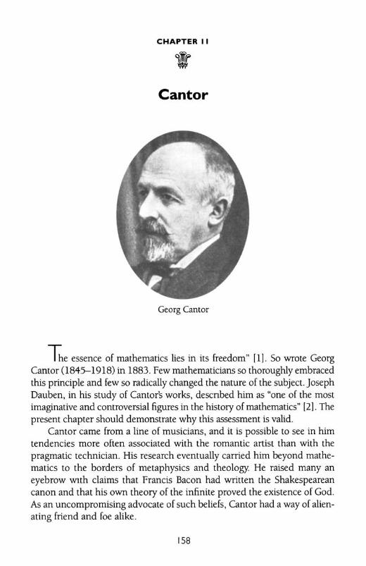
CHAPTER II

Cantor

Georg Cantor

~e essence of mathematics lies in its freedom" [1]. So wrote GeorgCantor (1845-1918) in 1883. few mathematicians so thoroughly embracedthis principle and few so radically changed the nature of the subject. JosephDauben, in his study of Cantor's works, descnbed him as "one of the mOStimaginative and controversial figures in the history of mathematics" [21. Thepresent chapter should demonstrate why this assessment is valid.

Cantor came from a line of musicians, and it is possible to see in himtendencies more often associated with the romantic artist than with thepragmatic technician. His research eventually carried him beyond mathe­matics to the borders of metaphysics and theology. He raised many aneyebrow Wlth claims that Francis Bacon had written the Shakespeareancanon and that his own theory of the infinite proved the existence of God.As an uncompromising advocate of such beliefs, Cantor had a way of alien­ating friend and foe alike.

158

CANTOR [59

Meanwhile, his life was troubled. He suffered bouts of severe depres­sion, almost certainly a bipolar disorder whose recurrences robbed him ofthe "mental freshness" he so coveted [3]. Time and again Cantor was sent towhat were called neuropathic hospitals to endure whatever treatment theycould offer. In 1918 he died in a psychiatric institution after a life withmore than its share of unhappiness.

None of this detracts from Cantors mathematical triumph. For all ofhis misfortune, Georg Cantor revolutionized the subject whose freedomhe so loved.

THE COMPLETENESS PROPERTY

As a young man, Cantor had studied with Weierstrass at the Universityof Berlin. There he wrote an 1867 dissertation on number theory, a fieldvery different from that for which he would become known. His researchled him to Fourier series and eventually to the foundations of analysis.

As we have seen, developments in the nineteenth century placed cal­culus squarely upon the foundation of limits. It had become clear that lim­its, in turn, rested upon properties of the real number system, foremostamong which is what we now call completeness. Today's students mayencounter completeness in different but logically equivalent forms, such as:

Cl. Any nondecreasing sequence that is bounded above con­verges to some real number.

C2. Any Cauchy sequence has a limit.C3. Any nonempty set of real numbers with an upper bound has

a least upper bound.

Readers in need of a quick refresher are reminded that {xk} is a Cauchysequence if, for every c> 0, there exists a whole number N such that, if mand n are whole numbers greater than or equal to N, then IXm - xnl < c. Inwords, a Cauchy sequence is one whose terms get and stay close to oneanother. This idea put in a brief appearance in chapter 6.

Likewise, M is said to be an upper bound of a nonempty set A if a ~ Mfor all elements a in A, and A is a least upper bound, or supremum, of A if(1) A is an upper bound of A and (2) if M is any upper bound of A, thenA~ M. These concepts appear in any modern analysis text.

There is one other version of completeness, cast in terms of nestedintervals, that will play an important role in the next few chapters. Again,we need a few definitions to clarify what is going on.

160 CHAPTER I I

A closed interval [a, bl is nested within [A, Bl if the former is a subsetof the latter. This amounts to nothing more than the condition that A ~

a ~ b ~ B. Suppose further that we have a sequence of closed, boundedintervals, each nested WIthin its predecessor, as in [a j , bd ~ [a2 , b21~[a3 , b31~ ... ~ [ak, bkl ~ .... Such a sequence is said to be descending.With this we can introduce another version of completeness:

C4. Any descending sequence of closed, bounded intervals has apoint that belongs to each of the intervals.

It is worth recalling why the intervals in question must be both closedand bounded. The descending sequence of closed (but not bounded)intervals

[1, 00) ~ [2, 00) ~ [3, 00) ~ ... ~ [k, 00) ~ ...

has no point common to all of them, and the descending sequence ofbounded (but not closed) intervals

(0, 1) ~ (0, 1/2) ~ (0, 1/3) ~ ... ~ (0, 11k) ~ ...

likewise has an empty intersection (to use set-theoretic terminology).Although our nineteenth century predecessors often neglected such dis­tinctions, we shall arrange for our intervals to be both closed and boundedbefore applying C4.

Each of these four incarnations of completeness guarantees that somereal number exists, be it the limit to which a sequence converges, or theleast upper bound that a set possesses, or a point common to each of a col­lection of nested intervals. As mathematicians probed the logical founda­tions of calculus, they realized that such existence was often sufficient fortheir theoretical purposes. Rather than identify a real number explicitly, itmay be enough to know that a number is out there somewhere. Com­pleteness provides that assurance.

One might ask: if the completeness property is so important, how dowe prove it? The answer required mathematicians to understand the realnumber system itself. From the whole numbers, it is a straightforward taskto define the integers (positive, negative, and zero) and from there to definethe rationals. But can we create the real numbers from more elementarysystems, just as the rationals were defined in terms of the integers?

Affirmative answers to this question came from Cantor and, inde­pendently, from his friend Richard Dedekind 0831-1916). Cantor's

CANTOR 161

construction of the reals was based on equivalence classes of Cauchysequences of rational numbers. Dedekind's approach employed partitionsof the rationals into disjoint classes, the so-called "Dedekind cuts." A thor­ough discussion of these matters would carry us far afield, for construct­ing the real numbers from the rationals is a bit esoteric for this book and,truth be told, a bit esoteric for most analysis courses. Nonetheless, Cantorand Dedekind did it successfully and then used their ideas to prove thecompleteness property as a theorem in their newly created realm.

This achievement can be seen as the final step in the separation ofcalculus from geometry. Dedekind and Cantor had gone back to the arith­metic basics-the whole numbers-from which the reals, then the com­pleteness property, and eventually all of analysis could be developed.Their achievement received the apt but nearly unpronounceable moniker:"the arithmetization of analysis."

THE NONDENUMERABILITY OF INTERVALS

It is not for defining the real numbers that Cantor has been chosen toheadline this chapter. Rather it is for his 1874 paper, "Uber eine Eigenschaftdes Inbegriffes aller reellen algebraischen Zahlen" (On a Property of the Total­ity of All Real Algebraic Numbers) [4]. This was a landmark in the historyof mathematics, one that demonstrated, in Daubens words, "[Cantors] giftfor posing incisive questions and for sometimes finding unexpected, evenunorthodox answers" [5].

Oddly, the significance of the paper was obscured by its title, for theresult about algebraic numbers was but a corollary, albeit a most interest­ing one, to the paper's truly revolutionary idea. That idea, simply stated, isthat a sequence cannot exhaust an open interval of real numbers. As weshall see, Cantor's argument involved the completeness property, thusplacing it properly in the domain of real analysis.

Theorem: If {xII} is a sequence of distinct real numbers, then any open,bounded interval (a, {3) of real numbers contains a point not includedamong the {xh}.

Proof: Cantor began with an interval (a, {3) and considered the sequencein consecutive order: Xl' X2 , X 3, X4 , .... If none orJust one of these termslies among the infinitude of real numbers in (a, {3), then the propositionis trivially true.

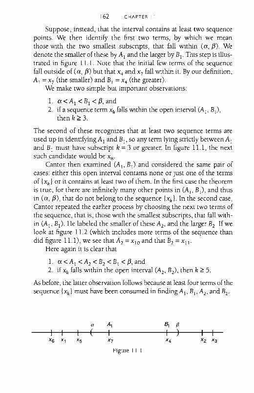
162 CHAPTER I I

Suppose, instead, that the interval contains at least two sequencepoints. We then identify the first two terms, by which we meanthose WIth the two smallest subscnpts, that fall WIthin (a, {3). Wedenote the smaller of these by Al and the larger by BI. This step is illus­trated in figure 11.1. Note that the initial few terms of the sequencefall outside of (a, {3) but that X4 and X7 fall WIthin it. By our definition,Al =x7 (the smaller) and BI =X4 (the greater).

We make two simple but important observations:

1. a<A I <BI <{3,and2. if a sequence term x" falls WIthin the open interval (AI' BI),

then k ~ 3.

The second of these recognizes that at least two sequence terms areused up in identifying Al and BI, so any term lying strictly between Aland BI must have subscript k = 3 or greater. In figure 11.1, the nextsuch candidate would be Xs '

Cantor then examined (AI' BI) and considered the same pair ofcases: either this open interval contains none or Just one of the termsof {x,,} or it contains at least two of them. In the first case the theoremis true, for there are infinitely many other points in (AI' Bj ), and thusin (a, {3), that do not belong to the sequence {x,,}. In the second case,Cantor repeated the earlier process by choosing the next two terms ofthe sequence, that is, those WIth the smallest subscripts, that fall with­in (AI' BI). He labeled the smaller of these A2, and the larger B2 If welook at figure 11.2 (which includes more terms of the sequence thandid figure ILl), we see that A2 =X lO and that B2 =Xjj'

Here again it is clear that

1. a < Al < A2 < B2 < BI < {3, and2. if x" falls WIthin the open interval (A2, B2), then k ~ 5.

As before, the latter observation follows because at least four terms of thesequence {x,,} must have been consumed in finding AI' Bj , A2, and B2.

a

(Xl

Figure 11 1

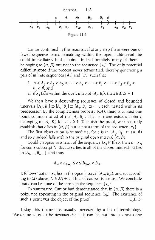
CANTOR 163

a At ~ 8 2 ~ f3I ( I I I I I )

X6 xl Xs Xg X7 XlO Xll X4 Xa X2 x3

Figure 11 2

Cantor continued in this manner. If at any step there were one orfewer sequence terms remaining within the open subinterval, hecould immediately find a point-indeed infinitely many of them­belonging to (a, /3) but not to the sequence IXh}' The only potentialdifficulty arose if the process never terminated, thereby generating apair of infinite sequences IA r } and IBr } such that

1. a < Al < A2 < A3 < ... < A r < ... < Br < ... < B3 < B2 <BI < /3, and

2. if xh falls within the open interval (A p Br), then k ~ 2r + 1

We then have a descending sequence of closed and boundedintervals [AI' BIl ;;;) [A2 , B2 l ;;;) [A 3 , B3 l ;;;) .. " each nested within itspredecessor. By the completeness property (C4), there is at least onepoint common to all of the [A p Brl. That is, there exists a point cbelonging to [Ap Brl for all r ~ 1. To finish the proof, we need onlyestablish that c lies in (a, /3) but is not a term of the sequence IXh }.

The first observation is immediate, for c is in [AI' BI ] c (a, /3)and so c indeed falls WIthin the original open interval (a, /3).

Could c appear as a term of the sequence IXh}? If so, then c =XNfor some subscript N Because c lies in all of the closed intervals, it liesin [AN+I' BN+I], and thus

It follows that c =X N lies in the open interval (AN' BN), and so, accord­ing to (2) above, N ~ 2N + 1. This, of course, is absurd. We concludethat c can be none of the terms in the sequence IXII} .

To summarize, Cantor had demonstrated that in (a, /3) there is apoint not appearing in the original sequence Ixh}' The existence ofsuch a point was the object of the proof. Q.E.D.

Today, this theorem is usually preceded by a bit of terminology.We define a set to be denumerable if it can be put into a one-to-one

164 CHAPTER I I

correspondence with the set of whole numbers. Sequences are tnviallydenumerable, with the required correspondence appearing as the sub­scripts. An infinite set that cannot be put into a one-to-one correspon­dence with the whole numbers is said to be nondenumerable. We thencharacterize the result above as proving that any open interval of realnumbers is nondenumerable.

The evolution of Cantors thinking on this matter is interesting.Through the early 1870s, he had pondered the fundamental properties ofthe real numbers, trying to isolate exactly what set them apart from therationals. Obviously, completeness was a key distinction that somehowembodied what was meant by "the continuum" of the reals.

But Cantor began to suspect there was a difference in the abundance ofnumbers in these two sets-what we now call their "cardinality"-and inNovember of 1873 shared with Dedekind his doubts that the whole num­bers could be matched in a one-to-one fashion with the real numbers.Implicitly this meant that, although both collections were infinite, thereals were more so.

Try as he might, Cantor could not prove his hunch. He wroteDedekind, in some frustration, "as much as I am inclined to the opinionthat [the whole numbers] and [the real numbers] permit no such uniquecorrespondence, I cannot find the reason" [6]. A month later, Cantor hada breakthrough. As a Christmas gift to Dedekind, he sent a draft of hisproof and, after receiving suggestions from the latter, cleaned it up andpublished what we saw above. Persistence had paid off.

Readers who know Cantor's "diagonalization" proof of nondenumer­ability may be surprised to see that his 1874 reasoning was wholly differ­ent. The diagonal argument, which Cantor described as a "much simplerdemonstration," appeared in an 1891 paper [7]. In contrast to the 1874proof, which, as we have seen, invoked the completeness property, diago­nalization was applicable to situations where completeness was irrelevant,far from the constraints of analysis proper.

Although the later argument is more familiar, the earlier one repre­sents the historic beginning and so has been included here. We stressagain that Cantor's original proof did not use terms like denumerabilitynor raise specific questions about infinite cardinalities. All this wouldcome later. In 1874, he simply showed that a sequence cannot exhaust anopen interval.

But why should anyone care? It was a good question, and Cantor hada spectacular answer.

CANTOR 165

THE EXISTENCE OF TRANSCENDENTALS, REVISITED

We recall that Cantor's paper was titled, "On a Property of the Totalityof All Real Algebraic Numbers." To this point, algebraic numbers have yetto be mentioned, nor have we said anything about the "property" of thesenumbers to which the title refers. The time has come to address thoseomISSIOns.

As we saw, a real number is algebraic if it is the solution to a polyno­mial equation with integer coefficients. There are infinitely many of these(for instance, any rational number), and it was no easy matter for Liouvilleto find a number that lay outside the algebraic realm.

Cantor, upon considering the matter, claimed that it was possible tolist the algebraic numbers in a sequence. At first glance, this may seempreposterous. It would require him to generate a sequence with the twinproperties that (1) every term was an algebraic number and (2) everyalgebraic number was somewhere in the sequence. A clever eye would benecessary to do this in an orderly and exhaustive fashion, but Cantor wasnothing if not clever. He began by introducing a new idea.

Definition: If P(x) = axn + bxn- l + cxn- 2 + ... + gx + h is an nth-degreepolynomial with integer coeffiCients, we define its height by (n - 1) +lal + Ibl + lei + ... + Ihl.

For instance, the height of P(x) = 2x3 - 4x2 + 5 is (3 - 1) + 2 + 4 + 5 = 13

and that of Q(x) =x6 - 6x4 - lOx3 + 12x2 - 60x + 17 is (6 - 1) + 1 + 6 +

10 + 12 + 60 + 17 = 111.Clearly the height of a polynomial with integer coefficients will itself

be a whole number. Further, any algebraic number has a minimal-degreepolynomial whose coefficients we can assume to have no common divisorother than 1. These conventions simplify the task at hand.

Cantor in turn collected all algebraic numbers that arise from polyno­mials of height 1, then those that arise from polynomials of height 2, thenof height 3, and so on. This was the key to arranging algebraic numbersinto an infinite sequence, here denoted by {ak }.

To see the process in action, we observe that the only polynomial withinteger coefficients of height 1 is P(x) =1 . Xl =x. The solution to theassociated equation P(x) =0 is the first algebraic number, namely a l =O.

166 CHAPTER I I

There are four polynomials with height 2:

Setting the first and second equal to zero yields the solution x =0, whichwe do not count again. Setting P3 (x) = 0 gives a2 = -1 and P4 (x) = 0 givesa3 = l.

We continue. There are eleven polynomials of height 3·

PI (x) = x3 , P2 (x) = 2x2 , P3 (x) = x2 + 1, P4 (x) = x 2 - 1,

Ps(x) =x2 +x, P6 (x) =x2 -x, P7 (x) = 3x, Ps(x) = 2x + 1,

Pg(x) = 2x - 1, PlO(x) =x + 2, Pll (x) =x - 2.

Upon setting these equal to zero, we get four new algebraic numbers:

1 1a 4 = - -, as = -, a6 = - 2, and a7 = 2.

2 2

As his title indicated, Cantor was restricting his attention to real algebraicnumbers, so 0 = P3 (x) =x2 + 1 added nothing to the collection.

And on we go. There are twenty-eight polynomials of height 4, andfrom these we harvest a dozen additional algebraic numbers, some ofwhich are irrational. For instance, the polynomial P(x) =x2 + x-I is of

-1+.J5 -1-.J5height 4 and contributes and ---

2 2As the heights increase, more and more algebraic numbers appear.

Conversely, any specific algebraic number must arise from some polyno­mial with integer coefficients, and this polynomial, in turn, has a height.

For instance, the algebraic number -Ii + V5, which we encountered in

chapter 8, is a solution to the polynomial equation x6 - 6x4 - 10x3 + 12x2 ­

60x + 17 =0 with height 11l.A few Simple observations allowed Cantor to wrap up his argument.

• For a given height, there are only finitely many polynomialsWlth integer coefficients.

• Each such polynomial can generate only finitely many newalgebraic numbers (because an nth-degree polynomial equationcan have no more than n solutions).

• Hence, for each height there can be only finitely many newalgebraic numbers.

CANTOR 167

This means that, upon "entering" a given height in our quest for algebraicnumbers, we must emerge from that height after finitely many steps. Wecannot get "stuck" in a height trying to list an infinitude of new algebraicnumbers.

Consequently, the number .J2 + V5 with its polynomial of heightIII has to show up somewhere in our sequence {all}' It will take a while,but the process must, after finitely many steps, bring us to height Ill, andthen, as we run through the polynomials of this height, we reach x6 - 6x4 ­

lOx3 + 12x2 - 60x + 17 after finitely many more. This will determine theposition of .J2 + V5 in the sequence {all}' The same can be said of anyreal algebraic number. So, the "property" of the algebraic numbers men­tioned in Cantor's title is, in modern parlance, its denumerability.

Now he combined his two results: first, that a sequence cannot exhaustan interval and, second, that the algebraic numbers form a sequence. Indi­Vldually, these are interesting. Together, they allowed him to conclude thatthe algebraic numbers cannot account for all points on an open interval.Consequently, Wlthin any Ca, f3), there must lie a transcendental.

Or, to put it directly, transcendental numbers exist.Of course, this was what Liouville had demonstrated a few decades

0011111earlier when he showed that ~ - - +-- + - +--+t 10k! - 10 102 106 1024

1 .---u:o + ... was transcendental. To prove the eXIstence of transcendental10numbers, he went out and found one.

Cantor reached the same end by very different means. Early in his1874 paper, he had promised "a new proof of the theorem first demon­strated by Liouville," and he certainly delivered [8]. But his argument, aswe have seen, contained no example of a specific transcendental. It wasstrikingly nonexplicit.

To contrast the two approaches, we offer the analogy of finding a nee­dle in a haystack. We enVlsion LiouVllle, industrious to a fault, putting onhis old clothes, hiking out to the field, and rooting around in the hay undera broiling sun. Hours later, drenched Wlth perspiration, he pncks his fingeron the elusive quarry; a needle! Cantor, by contrast, stays indoors usingpure reason to show that the mass of the haystack exceeds the mass of thehay in it. He deduces that there must be something else, that is, a needle, toaccount for the excess. Unlike LiouVllle, he remains cool and spotless.

Some mathematicians were troubled by a nonconstructive proof thatrelied upon the properties of infinite sets. Compared to Liouville's lengthy

168 CHAPTER I I

argument, Cantor's seemed too easy, almost like sleight-of-hand. Theyoung Bertrand Russell 0872-1970) may not have been alone in his ini­tial reaction to Cantors ideas:

I spent the time reading Georg Cantor, and copying out the gist ofhim into a notebook. At that time I falsely supposed all his argu­ments to be fallacious, but I nevertheless went through them all inthe minutest detail. This stood me in good stead when later on Idiscovered that all the fallacies were mine [9].

Like Russell, mathematicians came to appreciate Cantor for the inno­vator he was. His 1874 paper ushered in a new era for analysis, where theideas of set theory would be employed alongside the E - (j arguments ofthe Weierstrassians.

Cantor's work had consequences, many of which were truly astonish­ing. For instance, it is easy to show that if the algebraic numbers and thetranscendental numbers are each denumerable, then so is their union, theset of all real numbers. Because this is not so, Cantor knew that the tran­scendentals form a nondenumerable set and thus far outnumber theiralgebraic cousins. Eric Temple Bell put it this way: "The algebraic numbersare spotted over the plane like stars against a black sky; the dense black­ness is the firmament of the transcendentals" [10]. This is a delightfullyunexpected realization, for the plentiful numbers seem scarce, and thescarce ones seem plentiful. In a sense, Cantor showed that the transcen­dentals are the hay and not the needles.

A related but more far-reaching consequence was the distinctionbetween "small" and "large" infinite sets. Cantor proved that a denumer­able set, although infinite, was insignificantly infinite when compared to anondenumerable counterpart. As his ideas took hold, mathematicianscame to regard denumerable sets as so much jetsam, easily expendablewhen addressing questions of importance.

As we shall see, dichotomies between large and small sets would arisein other analytic settings. At the turn of the nineteenth century, Rene Bairefound a "large/small" contrast in what he called a set's "category," andHenri Lebesgue found another in what he called its "measure." Althoughcardinality, category, and measure are distinct concepts, each provided ameans of comparing sets that would prove valuable in mathematicalanalysis.

Cantor addressed other questions about infinite sets. One was, "Arethere nondenumerable sets having greater cardinality than intervals?" Thishe answered in the affirmative. Another was, "Are there infinite sets of an

CANTOR 169

intermediate cardinality between a denumerable sequence and a nonde­numerable interval?" This he never succeeded in resolving. With Cantor'sfounding VIsion and continuing research, set theory took on a life of itsown, quite apart from the concerns of analysis proper. But it all grew outof his 1874 paper.

Unlike many revolutionaries down through history, Georg Cantorlived to see his ideas embraced by the wider community. An early enthusi­ast was Russell, who described Cantor as "one of the greatest intellects ofthe nineteenth century" [11]. This is no small praise from a mathemati­cian, philosopher, and eventual Nobel laureate.

Another of Cantors admirers was the Italian prodigy Vito Volterra. Hiswork, which beautifully combined Weierstrassian analysis and Cantorianset theory, is the subject of our next chapter.

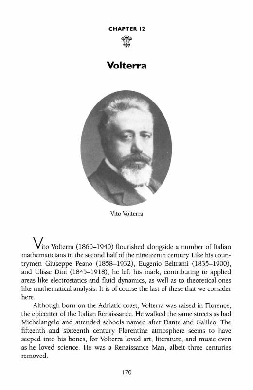
CHAPTER 12

'ItVolterra

Vito Volterra

~to Volterra (1860-1940) flourished alongside a number of Italianmathematicians in the second half of the nineteenth cemury. Like his coun­trymen Giuseppe Peano (1858-1932), Eugenio Beltrami (1835-1900),and Ulisse Dini (1845-1918), he left his mark, comnbuting to appliedareas like electrostatics and fluid dynamics, as well as to theoretical oneslike mathematical analysis. h is of course the last of these that we considerhere.

Although born on the Adriatic coast, Volterra was raised in Florence,the epicenter of the Italian Renaissance. He walked the same streets as hadMichelangelo and attended schools named after Dante and Galileo. Thefifteenth and sixteenth century Florentine atmosphere seems to haveseeped into his bones, for Volterra loved art, literature, and music evenas he loved science. He was a Renaissance Man, albeit three centuriesremoved.

170

VOLTERRA 171

Besides these pursuits, his political courage deserves to be celebrated.Witnessing the rise of Mussolini in the 1920s, Volterra took a publicstand in opposition and signed a declaration against the regime. This actultimately cost him his job but made him a hero for Italian intellectuals ofthe time. Upon his death in 1940, Italy had not yet shed its fascistscourge, but Volterra had fought the good fight in anticipation of a betterfuture.

If he showed great courage late in life, he had shown great precocityearly on. Young Volterra read college-level mathematics texts at age 11,impressed his teachers during adolescence, and somehow secured a posi­tion as a physics laboratory assistant at the University of Florence whilestill in high school. His academic career was spectacularly rapid, culmi­nating with a doctorate m physics at the age of 22 [1].

In this chapter we discuss a pair of Volterra's early discoveries, bothpublished in 1881, three years after his high school graduation The firstwas another in the growing list of pathological counterexamples, one thatturned up a previously unnoticed flaw in the Riemann integral. The sec­ond, almost paradoxically, was a theorem showing that pathology has itslimits, for Volterra proved that no function can be continuous at eachrational point and discontinuous at each irrational one. Such a functionwould simply be too pathological to exist. We shall examine the theoremin full, but we begin with a few words about the counterexample.

VOLTERRA'S PATHOLOGICAL FUNCTION

The second version of the fundamental theorem of calculus, which wesaw in chapter 6, was stated by Cauchy as follows: "If F is differentiable

and if its derivative F' is continuous, then s: F'(x)dx = F(b) - F(a)."

Informally, this says that under the nght conditions the integral of thederivative restores the original function. In the proof, Cauchy used thehypotheses that (a) F has a derivative and (b) this derivative is itself contin­uous. But were both necessary?

Statement (a) seems indispensable, for we could not hope to integratea derivative if the derivative fails to exist. But the status of (b) is more sus­pect Must we assume something as restrictive as the continuity of F' inorder for the result to hold?

This is not a trivial issue. On the one hand, we saw in chapter 10 thatthe continuity of a derivative cannot be taken for granted, for the function

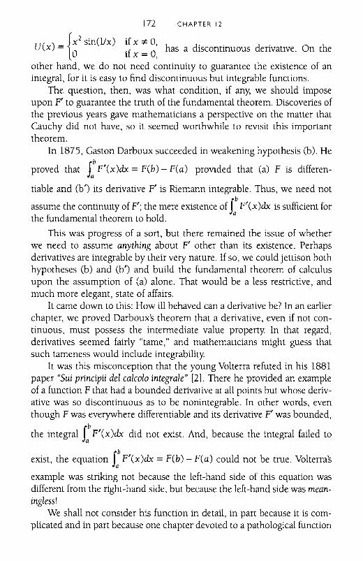
172 CHAPTER 12

U(x) = {X2

sin(lJx) if X :f. 0, has a discontinuous derivative. On theo if x = 0,

other hand, we do not need continuity to guarantee the existence of anintegral, for it is easy to find discontinuous but integrable functions.

The question, then, was what condition, if any, we should imposeupon F' to guarantee the truth of the fundamental theorem. Discoveries ofthe previous years gave mathematicians a perspective on the matter thatCauchy did not have, so it seemed worthwhile to reVIsit this importanttheorem.

In 1875, Gaston Darboux succeeded in weakening hypothesis (b). He

proved that 1:F'(x)dx = F(b) - F(a) provided that (a) F is differen­

tiable and (b') its derivative F' is Riemann integrable. Thus, we need not

assume the continuity of F'; the mere existence of1: F'(x)dx is sufficient forthe fundamental theorem to hold.

This was progress of a sort, but there remained the issue of whetherwe need to assume anything about F' other than its existence. Perhapsderivatives are integrable by their very nature. If so, we could jettison bothhypotheses (b) and (b') and build the fundamental theorem of calculusupon the assumption of (a) alone. That would be a less restrictive, andmuch more elegant, state of affairs.

It came down to this: How ill behaved can a derivative be? In an earlierchapter, we proved Darboux's theorem that a derivative, even if not con­tinuous, must possess the intermediate value property. In that regard,derivatives seemed fairly "tame," and mathematicians might guess thatsuch tameness would include integrability.

It was this misconception that the young Volterra refuted in his 1881paper "Sui principii del calcolo integrale" [2]. There he provided an exampleof a function F that had a bounded derivative at all points but whose deriv­ative was so discontinuous as to be nonintegrable. In other words, eventhough F was everywhere differentiable and its derivative F' was bounded,

the integral 1:F'(x)dx did not exist. And, because the integral failed to

exist, the equation 1:F'(x)dx = F(b) - F(a) could not be true. Volterra's

example was striking not because the left-hand side of this equation wasdifferent from the right-hand side, but because the left-hand side was mean­ingless!

We shall not consider his function in detail, in part because it is com­plicated and in part because one chapter devoted to a pathological function

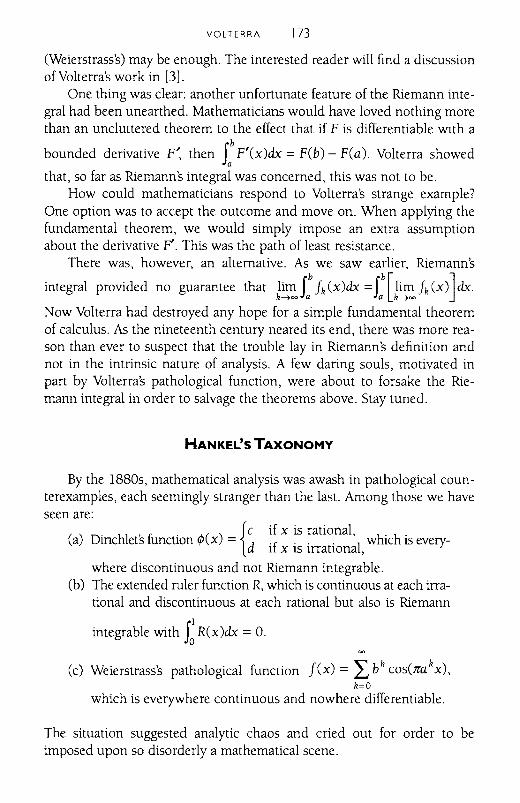
VOLTERRA 173

(Weierstrass's) may be enough. The interested reader will find a discussionof Volterra's work in [3].

One thing was clear: another unfortunate feature of the Riemann inte­gral had been unearthed. Mathematicians would have loved nothing morethan an uncluttered theorem to the effect that if F is differentiable WIth a

bounded derivative F', then s: F'(x)dx = F(b) - F(a). Volterra showed

that, so far as Riemann's integral was concerned, this was not to be.How could mathematicians respond to Volterra's strange example?

One option was to accept the outcome and move on. When applying thefundamental theorem, we would simply impose an extra assumptionabout the derivative F'. This was the path of least resistance.

There was, however, an alternative. As we saw earlier, Riemann's

integral provided no guarantee that lim rbfk (x)dx = rb

[lim fk (X)J dx.k~ooJa Ja k~oo

Now Volterra had destroyed any hope for a simple fundamental theoremof calculus. As the nineteenth century neared its end, there was more rea­son than ever to suspect that the trouble lay in Riemann's definition andnot in the intrinsic nature of analysis. A few daring souls, motivated inpart by Volterra's pathological function, were about to forsake the Rie­mann integral in order to salvage the theorems above. Stay tuned.

HANKEL'S TAXONOMY

By the 1880s, mathematical analysis was awash in pathological coun­terexamples, each seemingly stranger than the last. Among those we haveseen are:

, {c if x is rational,(a) Dinchlets function lP(x) = d ·f .. . I which is every-

1 x IS lrratlOna ,

where discontinuous and not Riemann integrable.(b) The extended ruler function R, which is continuous at each irra­

tional and discontinuous at each rational but also is Riemann

integrable with J~ R(x)dx = o.

(c) Weierstrass's pathological function f(x) = L bkcos(Jra kx),

k=O

which is everywhere continuous and nowhere differentiable.

The situation suggested analytic chaos and cried out for order to beimposed upon so disorderly a mathematical scene.

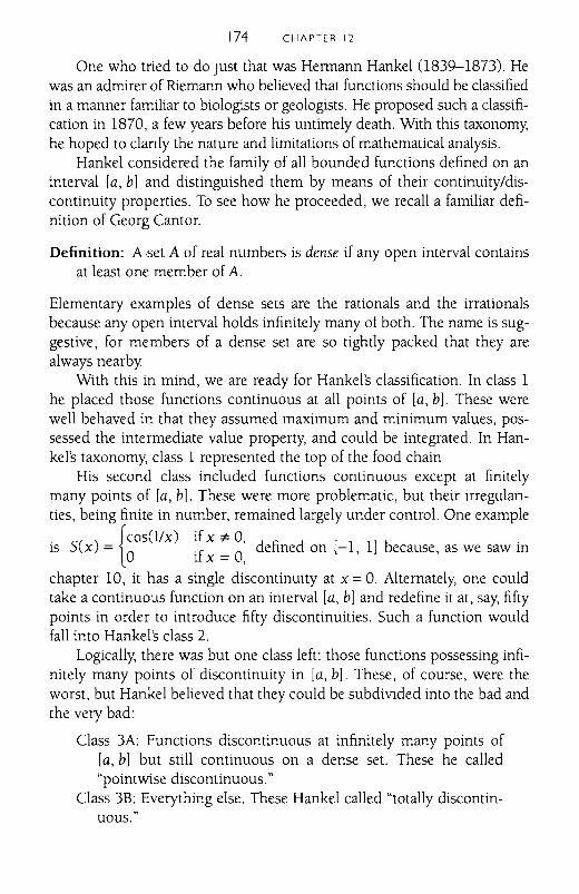
174 CHAPTER 12

One who tried to do Just that was Hermann Hankel 0839-1873). Hewas an admirer of Riemann who believed that functions should be classifiedin a manner familiar to biologists or geologists. He proposed such a classifi­cation in 1870, a few years before his untimely death. With this taxonomy,he hoped to clanfy the nature and limitations of mathematical analysis.

Hankel considered the family of all bounded functions defined on aninterval [a, b] and distinguished them by means of their continuity/dis­continuity properties. To see how he proceeded, we recall a familiar defi­nition of Georg Cantor.

Definition: A·set A of real numbers is dense if any open interval containsat least one member of A.

Elementary examples of dense sets are the rationals and the irrationalsbecause any open interval holds infinitely many of both. The name is sug­gestive, for members of a dense set are so tightly packed that they arealways nearby.

With this in mind, we are ready for Hankel's classification. In class 1he placed those functions continuous at all points of [a, b]. These werewell behaved in that they assumed maximum and minimum values, pos­sessed the intermediate value property, and could be integrated. In Han­kel's taxonomy, class 1 represented the top of the food chain

His second class included functions continuous except at finitelymany points of [a, b]. These were more problematic, but their irregulan­ties, being finite in number, remained largely under control. One example

{cosel/x) if x *- 0,

is Sex) = 0 if x = 0, defined on [-1, 1] because, as we saw in

chapter 10, it has a single discontinuity at x =O. Alternately, one couldtake a continuous function on an interval [a, b] and redefine it at, say, fiftypoints in order to introduce fifty discontinuities. Such a function wouldfall into Hankel's class 2.

Logically, there was but one class left: those functions possessing infi­nitely many points of discontinuity in [a, b]. These, of course, were theworst, but Hankel believed that they could be subdiVlded into the bad andthe very bad:

Class 3A: Functions discontinuous at infinitely many points of[a, b] but still continuous on a dense set. These he called"pointwise discontinuous."

Class 3B: Everything else. These Hankel called "totally discontin­uous."

VOLTERRA 175

We see that a pointwise discontinuous function in class 3A, in spiteof its infinitude of discontinuities, must be continuous somewhere in anyopen interval. On the other hand, for a function in class 3B theremust exist some open subinterval (c, d) within (a, b) where the functionhas no point of continuity at all. A totally discontinuous functionthus features a solid subinterval featuring nothing but points of discon­tinuity.

Where do the three pathological functions cited above fit into Han­kel's scheme? Dirichlet's function, being discontinuous everywhere, fallsinto class 3B as totally discontinuous. The ruler function is discontinuousat infinitely many points (the rationals) yet continuous on a dense set (theirrationals) and consequently belongs to class 3A as pointWIse discontinu­ous. And Weierstrass's function, perhaps the weirdest of all, is paradoxi­cally in class 1, for it is continuous everywhere.

Hankel found his classification important in the folloWIng sense: heknew that functions in class 1 and in class 2 are Riemann integrable, andthe examples at his fingertips of pointwise discontinuous functions wereintegrable as well. By contrast, Dirichlet's totally discontinuous functionwas not. To him, the gap between classes 3A and 3B seemed to be theunbridgeable chasm. As Thomas Hawkins put it, "By making the distinc­tion between pointWIse and totally discontinuous functions, Hankelbelieved he had separated the functions amenable to mathematical analy­sis from those beyond its reaches" [4].

To demonstrate the value of all this, Hankel proved a spectacular the­orem: a bounded function on [a, b] was Riemann integrable if and only ifit was no worse than pointwise discontinuous. That is, proVIded it fell intoclass 1, class 2, or class 3A, a bounded function could be integrated; thosethat occupied class 3B were not integrable and, by extension, analyticallyhopeless.

Hankel's theorem appeared to answer the major question we intro­duced earlier: "How discontinuous can an integrable function be?"The answer, according to him, was, "at worst pointwise discontinuous."His proof showed that, so long as a function was continuous on adense set, all those discontinuities would not matter in terms of inte­grability. This was exactly the kind of simple result mathematicians hadlonged for.

Unfortunately, it was also incorrect.With ideas this complicated, even great scholars can make mistakes,

and Hankel made a doozy. To be fair, half of his theorem was true: if afunction is Riemann integrable, it must indeed be continuous on a dense

176 CHAPTER 12

set. A totally discontinuous function, haVIng a solid subinterval of pointsof discontinuity, cannot possess a Riemann integral. Again, one thinks ofDirichlet's function in this regard.

But Hankel's proof of the converse was flawed. In 1875, the Britishmathematician H. j. S. Smith (1826-1883) published an example of apointwise discontinuous but non-integrable function which, he said,"deserves attention because it is opposed to a theory of discontinuousfunctions which has received the sanction of an eminent geometer,Dr. Hermann Hankel, whose recent death at an early age is such a greatloss to mathematical science" [5]. Smith's example was nontrivial, requir­ing the construction of what we now call a nowhere dense set of positivemeasure. We refer those seeking details to Hawkins [6]. For now, wemerely observe that the link between continuity and Riemann integrabilityremained unclear, and the question of how discontinuous an integrablefunction could be was still open. PointWIse discontinuity, whatever itsvalue, did not provide the long-sought connection.

Nonetheless there had been progress of a sort. Riemann had extendedthe notion of integrability to include some highly discontinuous func­tions, and the true half of Hankel's theorem, along with Smith's counterex­ample, showed that the Riemann-integrable functions were properlyembedded within the larger collection of functions that were continuouson a dense set.

We note in passing that the term "pointWIse discontinuous" has some­times been carelessly taken to mean "at worst pointWIse discontinuous."That is, all functions in Hankel's classes 1, 2, or 3A were lumped under thesingle rubric of pointwise discontinuity, which led to the bizarre situationof placing the continuous functions (class 1) among the "pointwise dis­continuous" ones. Because the common property of functions in thesefirst three classes is that each is continuous on a dense set, we might sug­gest densely continuous as an umbrella term to include all functions inclasses 1, 2, and 3A.

In any case, Hankel's taxonomy initially seemed to be a promisingvehicle for carving apart the analytically accessible functions from the ana­lytically intractable ones. As it turned out, however, many of thoseintractable functions could be handled quite nicely within the context ofset theory and the Lebesgue integral. Nowadays, Hankel's distinctionshave largely fallen by the wayside.

But in the late nineteenth century, pointwise discontinuity remained atopiC of research capable of engaging the most talented mathematicians.One of these was the 21-year-old Vito Volterra.

VOLTERRA 177

THE LIMITS OF PATHOLOGY

The epidemic of pathological functions suggested that any behavior,no matter how bizarre, could be realized by an ingeniously constructedexample from a suitably inventive mathematician.

Who, for instance, could envision the ruler function, continuous ateach irrational point and discontinuous at each rational one? And why notsuppose that somewhere, waiting to be discovered, lay an equally peculiarfunction continuous at each rational point and discontinuous at each irra­tional? One seemed no more outlandish than the other.

That continuity and discontinuity points can sometimes be inter­changed is evident in the following examples. First define

H() {X if x "* 0, Th·· b· I· 11· b h .x = 1 if x = O. IS IS 0 VIOUS Ycontmuous at a pomts ut t e OrI-

gin, where it has its lone point of discontinuity

. . {x 2 if x is rational .As ItS counterpart, we mtroduce K(x) = .f... '1 It IS noto 1 x IS IrratlOna .

difficult to see that K is discontinuous at any a"* O. For, if we let {Xk}be a sequence of rationals converging to a and {Yk} be a sequence of

irrationals converging to a, then lim K(xk) = lim (x~) = a2, whereas

k~= k~=

lim K(Yk) = lim 0 = 0 "* a2. Because these sequential limits differ, we

k~= k~=

know that lim K(x) cannot exist and so K is discontinuous at x = a.x~a

However, for any x, be it rational or irrational, we have 0 ~ K(x) ~ x 2 ,

and so a simple squeezing argument shows that lim K(x) = 0 = K(O). Itx~O

follows that K is a function with a lone point of continuity: the origin. So,for Hand K as defined here, the points of continuity and of discontinuityhave been swapped.

In this regard, it will be useful to introduce the following.

Definition: For a function f, we let Cf ={x If is continuous at x} andOf ={xlf is discontinuous at x}.

Our previous discussion can be neatly summarized by: CH = {xlx"* O} =OK and CK = {a} =0H·

The issue of interchanging continuity and discontinuity points is anintriguing one. For any function f, is there a "complementary" function g

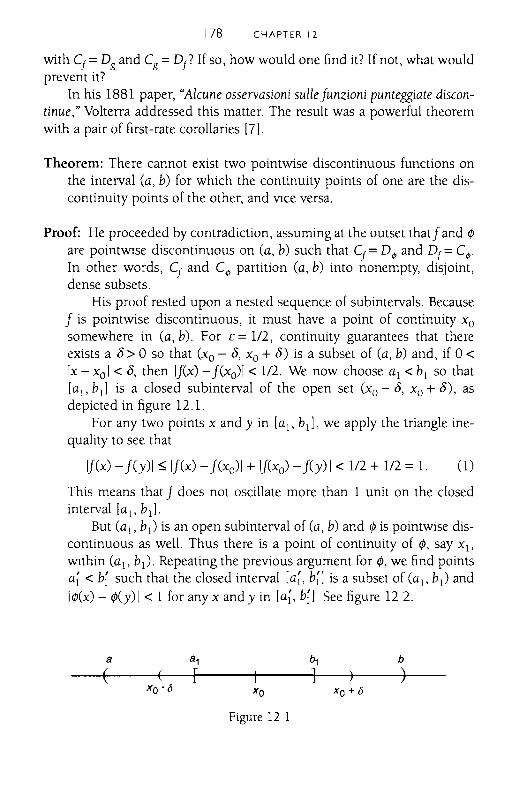
a

178 CHAPTER 12

with Cf =Dg and Cg =Of? If so, how would one find it? If not, what wouldprevent it?

In his 1881 paper, "Alcune osservasioni sulle funzioni punteggiate discon­tinue," Volterra addressed this matter. The result was a powerful theoremwith a pair of first-rate corollaries [7].

Theorem: There cannot exist two pointwise discontinuous functions onthe interval Ca, b) for which the continuity points of one are the dis­continuity points of the other, and VIce versa.

Proof: He proceeded by contradiction, assuming at the outset thatf and ¢are pointWIse discontinuous on Ca, b) such that Cf = 04> and Of = C4>'In other words, Cf and C4> partition Ca, b) into nonempty, disjoint,dense subsets.

His proof rested upon a nested sequence of subintervals. Becausef is pointwise discontinuous, it must have a point of continuity Xosomewhere in Ca, b). For E = 1/2, continuity guarantees that thereexists a 0> 0 so that CXo - 0, Xo + 0) is a subset of Ca, b) and, if 0 <Ix - xol < 0, then IfCx) - j(xo)I < 1/2. We now choose a j < b l so that[a j, b j ] is a closed subinterval of the open set CXo - 0, Xo + 0), asdepicted in figure 12.1.

For any two points x and y in [a j, b j ], we apply the triangle ine­quality to see that

IfCx) - fCy)1 ~ IfCx) - fCxo)I+ IfCxo) - fCy) I < 1/2 + 1/2 = 1. (1)

This means that f does not oscillate more than 1 unit on the closedinterval raj, bd.

But Cal, bj ) is an open subinterval of Ca, b) and ¢ is pointwise dis­continuous as well. Thus there is a point of continuity of ¢, say x j,WIthin Ca j, b j ). Repeating the previous argument for ¢, we find pointsa~ < b~ such that the closed interval [a~, b{] is a subset of Ca j, bl ) andI¢Cx) - ¢Cy)1 < 1 for any x andy in [a~, b;J See figure 122.

~ ~ b--f.(--f-(-----l[~-_+_--]--+----1)I---­

Xo - <5

Figure 12 1

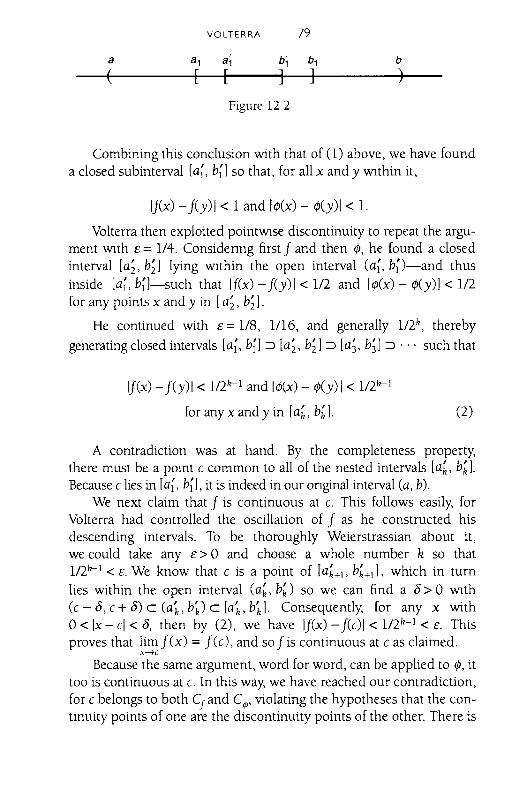
a

(

VOLTERRA [79

Figure 122

b

)

Combining this conclusion with that of (1) above, we have founda closed subinterval [a~, b~] so that, for all x and y Wlthin it,

Ij(x) - j(y)1 < I and Il/>(x) - l/>(y)I< 1.

Volterra then exploited pointWlse discontinuity to repeat the argu­ment Wlth E = 1/4. Considenng first j and then l/>, he found a closedinterval [a;, b;] lying Wlthin the open interval (a~, b~)-and thusinside [a~, bn-such that Ij(x) - j(y) I < 1/2 and Il/>(x) -l/>(y)1 < 1/2for any points x and y in [a;, b;].

He continued with E = 1/8, 1/16, and generally 1/2k, thereby

generating closed intervals [a~, b~]::::> [a;, b;J::::> [a;, b;J::::>··· such that

Ij(x) - j(y)1 < 1/2k- 1 and Il/>(x) -l/>(y) 1< 1/2k- 1

for any x and y in [a~, b~ 1. (2)

A contradiction was at hand. By the completeness property,there must be a pomt c common to all of the nested intervals [a~, b~ 1.Because c lies in [a~, b~l, it is indeed in our onginal interval (a, b).

We next claim that j is continuous at c. This follows easily, forVolterra had controlled the oscillation of j as he constructed hisdescending intervals. To be thoroughly Weierstrassian about it,we could take any E> 0 and choose a whole number k so that1/2k- 1 < E. We know that c is a point of [a~+l' b~+l], which in turnlies within the open interval (a~, b~) so we can find a 8> 0 Wlth(c - 8, c + 8) c (a~, b~) c [a~, b~]. Consequently, for any x with0< Ix - cl < 8, then by (2), we have Ij(x) - j(c)1 < 1/2h- 1 < E. Thisproves that lim j(x) = j(c), and so j is continuous at c as claimed.

X---7C

Because the same argument, word for word, can be applied to l/>, ittoo is continuous at c. In this way, we have reached our contradiction,for c belongs to both Cf and C tP , violating the hypotheses that the con­tinuity points of one are the discontinuity points of the other. There is

180 CHAPTER 12

no alternative but to conclude that two such pointwise discontinuousfunctions cannot exist. Q.E.D.

Before proceeding, we make a pair of observations. The first is thatVolterra was vague about insisting that the intervals [a~, b~ Ibe closed. Thisis an omission easily repaired, as we have done. Second, in the exampleabove where the continuity points of H are the discontinuity points of Kand vice versa, we note that K is totally discontinuous (Hankers class 3B)rather than pointwise discontinuous (Hankers class 3A). Consequently­lest anyone lose sleep on this account-that example in no way contra­dicts Volterra's result.

He followed his theorem with two important corollaries. The first,which settled a major question of analysis, was stated as follows:

Because we have a function continuous at each irrational pointand discontinuous at each rational, it will be impossible to find afunction that is discontinuous at each irrational point and contin­uous at each rational. [81

To flesh out his argument, we imagine a function G for which CG isthe (dense) set of rationals. Then G is pointwise discontinuous. But wehave previously encountered the extended ruler function R which ispointWIse discontinuous as well, with CR being the set of irrationals. Thecontinuity points of G would then be the discontinuity points of R, in con­tradiction to Volterras theorem. Consequently, it is impossible for bothfunctions to exist. Because the ruler function most certainly does exist, weare forced to conclude that the function G does not. Volterra's theoremdemonstrated, in the parlance of a Western movie, that "this town is notbig enough for both of them." A function continuous only on the rationalsis a logical impossibility.

Pathology, then, has its limits. No matter how clever the mathemati­cian, certain functions remain beyond the pale, a fact Volterra demonstratedwith this clever argument. But he had one more corollary up his sleeve,that there can be no continuous function taking rationals to irrationalsand VIce versa [9].

Corollary: There does not exist a continuous function g defined on thereal numbers such that g(x) is rational when x is irrational and g(x) isirrational when x is rational.

VOLTERRA 181

Proof: Again, for the sake of contradiction, Volterra assumed such afunction g exists. We then define G by G(x) = R(g(x», where R isthe extended ruler function from above, and make two claimsabout G:

Claim 1: If x is rational, G is continuous at x.

This is eVIdent because, if x is rational, g(x) is irrational, so R is con­tinuous at g(x). But g is assumed to be continuous everywhere, so thecomposite function G will be continuous at x.

Claim 2: If y is irrational, then G is discontinuous at y.

This is easily verified by choosing a sequence {xk} of rationals con­verging to y. Then

lim G(Xk) = lim R(g(Xk» = lim a = 0,k~= k~= k~=

because g carries each rational xk to an irrational g(Xk), and the rulerfunction is zero at irrational points. On the other hand, G(y) =R(g(y» :I; a because g(y) is rational. In short, lim G(Xk) -::;:. G(y), andso G is discontinuous at y. k~=

Taken together, these claims show that G is continuous upon therationals and discontinuous upon the irrationals-a situation thatVolterra had just proved to be impossible! It follows that a functionlike g cannot exist. There is no continuous transformation that carriesrationals to irrationals and vice versa. Q.E.D.

Among other things, these results remind us that the rationals andirrationals, although both dense sets of real numbers, are intrinsicallynoninterchangeable. As we saw, Cantor had highlighted the fact that therationals are denumerable and the irrationals are not, but mathematicianswould find other, more subtle distinctions between these systems. One ofthese was the notion of a set's "category," a concept due to Volterras giftedstudent Rene Baire, who is the subject of our next chapter.

With this, we leave the 21-year-old Vito Volterra. A long and distin­guished career lay ahead of him, one that would see continued mathematicalsuccess, international recognition, and even an honorary knighthood fromBritain's King George V

Looking back from later in his life, Volterra characterized the 1800s as"the century of the theory of functions" [10]. Starting with Euler's initial

[82 CHAPTER 12

ideas, the concept of function had assumed a central role in the work ofCauchy, Riemann, and Weierstrass and then been passed to the generationof Cantor, Hankel, and Volterra himself. Functions had come to dominateanalysis, and their unexpected possibilities surprised mathematicians timeand again. As we have seen, Volterra deserves a place in this tale for twodifferent but fascinating discoveries from 1881.

For such a young man, it had been quite a year.

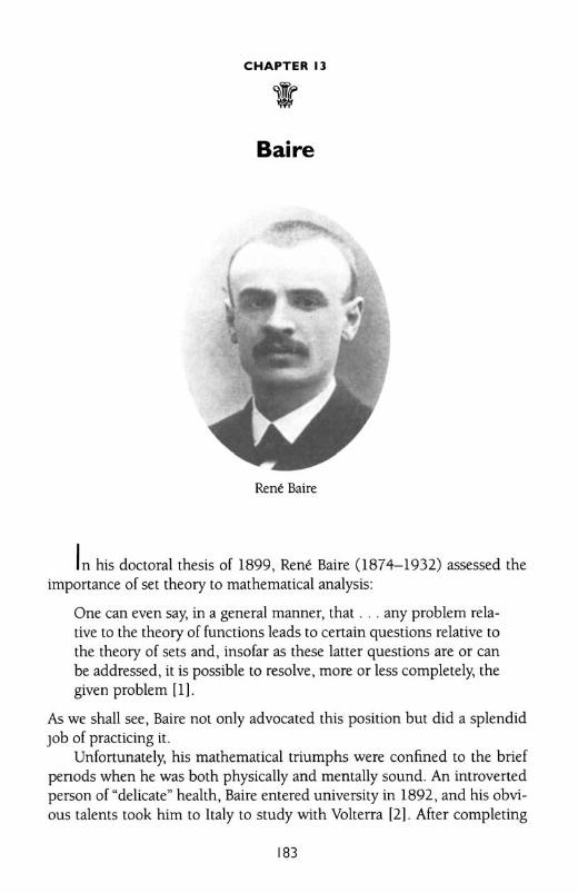
CHAPTER 13

t'Baire

Rene Baire

In his doctoral thesis of 1899, Rene Baire 0874-1932) assessed theimportance of set theory to mathematical analysis:

One can even say. in a general manner, that ... any problem rela­tive LO the theory of functions leads to cenain questions relative to

the theory of sets and, insofar as these latter questions are or canbe addressed, it is possible to resolve, more or less completely, thegiven problem Ill.

As we shall see, Baire not only advocated this position but did a splendidJob of practicing it.

Unfonunately, his mathematical triumphs were confined to the briefpenods when he was both physically and mentally sound, An introvertedperson of ~delicate" health, Baire entered university in 1892, and his obvi­ous talents LOok him to Italy to study with Volterra [2]. After completing

183

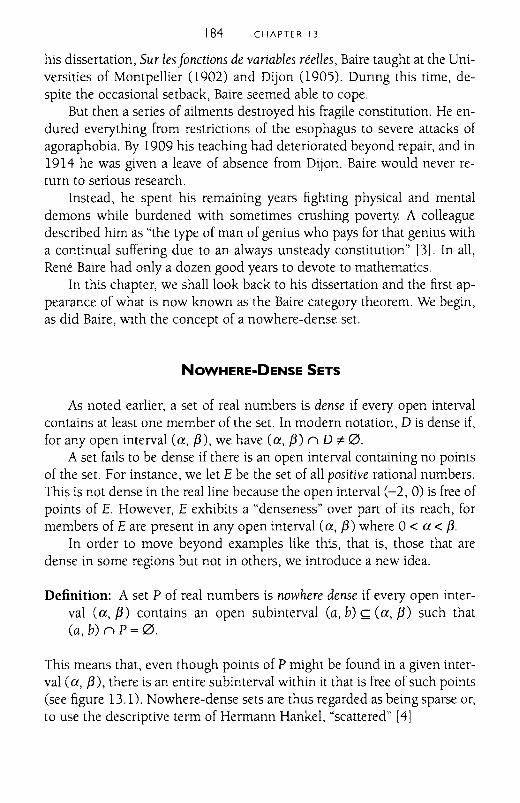
184 CHAPTER 13

his dissertation, Sur les fonctions de variables rt~el1es, Baire taught at the Uni­versities of Montpellier (1902) and Dijon (1905). Dunng this time, de­spite the occasional setback, Baire seemed able to cope.

But then a series of ailments destroyed his fragile constitution. He en­dured everything from restrictions of the esophagus to severe attacks ofagoraphobia. By 1909 his teaching had deteriorated beyond repair, and in1914 he was given a leave of absence from Dijon. Baire would never re­turn to serious research.

Instead, he spent his remaining years fighting physical and mentaldemons while burdened with sometimes crushing poverty. A colleaguedescribed him as "the type of man of genius who pays for that genius witha continual suffering due to an always unsteady constitution" [3]. In all,Rene Baire had only a dozen good years to devote to mathematics.

In this chapter, we shall look back to his dissertation and the first ap­pearance of what is now known as the Baire category theorem. We begin,as did Baire, WIth the concept of a nowhere-dense set.

NOWHERE-DENSE SETS

As noted earlier, a set of real numbers is dense if every open intervalcontains at least one member of the set. In modern notation, D is dense if,for any open interval (a, /3), we have (a, /3) II D"* 0.

A set fails to be dense if there is an open interval containing no pointsof the set. For instance, we let E be the set of all positive rational numbers.This is not dense in the real line because the open interval (-2,0) is free ofpoints of E. However, E exhibits a "denseness" over part of its reach, formembers of E are present in any open interval (a, /3) where 0 < a < /3.

In order to move beyond examples like this, that is, those that aredense in some regions but not in others, we introduce a new idea.

Definition: A set P of real numbers is nowhere dense if every open inter­val (a, /3) contains an open subinterval (a, b) ~ (a, /3) such that(a,b)IIP=0.

This means that, even though points of P might be found in a given inter­val (a, /3), there is an entire subinterval within it that is free of such points(see figure 13.1). Nowhere-dense sets are thus regarded as being sparse or,to use the descriptive term of Hermann Hankel, "scattered" [4]

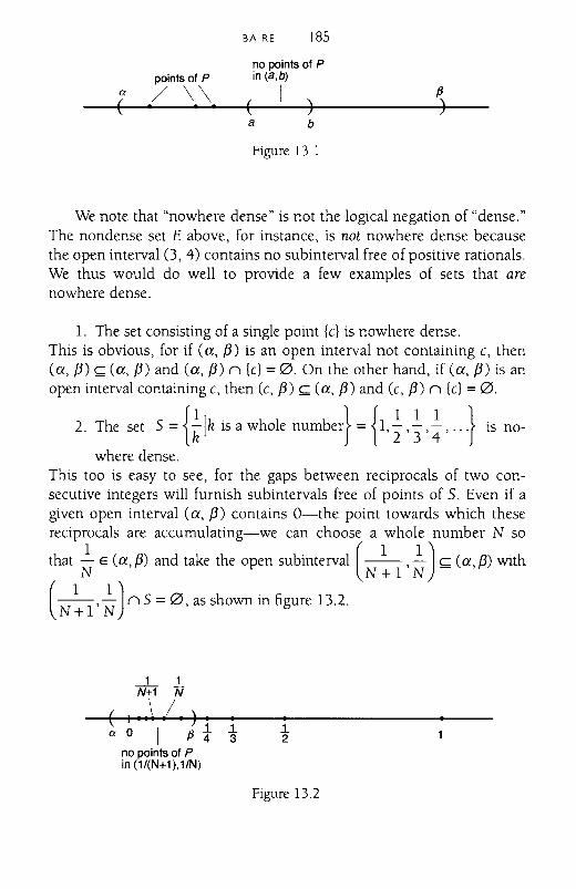
BAIRE 185

points of P

( / \ \

no points of Pin (a,b)

( [ ) fJ)

a b

Figure 13 1

We note that "nowhere dense" is not the logical negation of "dense."The nondense set E above, for instance, is not nowhere dense becausethe open interval (3, 4) contains no subinterval free of positive rationals.We thus would do well to provide a few examples of sets that arenowhere dense.

1. The set consisting of a single point {e} is nowhere dense.This is obvious, for if Ca, 13) is an open interval not containing c, thenCa, 13) ~ Ca, 13) and Ca, 13) n {c} = 0. On the other hand, if Ca, 13) is anopen interval containing c, then Cc, 13) ~ Ca, 13) and Cc, 13) n {c} = 0.

2. The set s={ilk isawhole number}={l,±,l,l,··} is no-

where dense.This too is easy to see, for the gaps between reciprocals of two con­secutive integers will furnish subintervals free of points of S. Even if agiven open interval Ca, 13) contains O-the point towards which thesereciprocals are accumulating-we can choose a whole number N so

that ~ E Ca,f3) and take the open subinterval (_1_,~) c Ca, 13) withN N+1 N -

(_1_,~) n 5 = 0, as shown in figure 13.2.N+1 N

1­2aO I fJt~

no points of Pin (1/(N+1),1/N)

_1_ 1N+1 N\ /( I···· .). ·

Figure 13.2

[86 CHAPTER 13

3. The set T ={~ +tIr and k are whole numbers} is nowhere dense.

To conjure up a mental picture of this set, fix r and let k run through the1 111111

positive integers. This generates points - + 1, - + - ,- + - ,- + - , ... ,whichr r2r3r4

1cluster around - in the same way that the points of the previous example

r

1clustered around O. Because r is arbitrary, every reciprocal - is such a cluster

rpoint, giVIng T quite a complicated structure. Nonetheless, the gaps among

1 1the points - + - are such as to make Tnowhere dense Cwe omit the details).

r k

Before seeing what Baire made of this, we prove two simple lemmasthat will come in handy.

Lemma 1: Subsets of nowhere-dense sets are nowhere dense. That is, if Pis a nowhere-dense set and U ~ P, then U is nowhere dense.

Proof: Given an open interval Ca, {3), we know there exists an opensubinterval Ca, b) ~ Ca, {3) with Ca, b) n P =0. Because U is a sub­set of P, it is clear that Ca, b) n U =0, and so U is nowhere dense aswell. Q.E D.

Lemma 2: The union of two nowhere-dense sets is nowhere dense

Proof: Let PI and P2 be nowhere dense. To show that PI U P2 is alsonowhere dense, we begin with an open interval Ca, {3). Because PI isnowhere dense, there exists an open subinterval Ca, b) ~ Ca, {3) withCa, b) n PI =0. But Ca, b) is itself an open interval and P2 is nowheredense, so there is an open subinterval Cc, d) ~ Ca, b) ~ Ca, {3) withCc, d) n P2 =0. Clearly, Cc, d) is an open subinterval of Ca, {3) con­taining no points of PI or P2· Thus, Cc, d) n CPI U P2) =0, so PI U P2is nowhere dense. Q E.D.

As this second lemma shows, we can amalgamate two-or for thatmatter any finite number-of nowhere-dense sets and still find ourselveswith a nowhere-dense outcome. Even the union of a million such setswould remain, in Hankel's terminology, scattered.

BAIRE 187

But what if we assemble an irifinitude of nowhere-dense sets? Whatsort of structure might such a union have? And what use might this be tomathematical analysis? These are matters that Baire addressed with hischaracteristic ingenuity.

THE BAIRE CATEGORY THEOREM

In his thesis, Baire wrote of a set F with the property that

there exists a denumerable infinity of sets PI' P2' P3' P4' ... , eachnowhere dense, such that every point [of F] belongs to at least oneof the sets PI' P2 , P3 , P4 , .... I will say a set of this nature is of thefirst category. [5]

In other words, F is a set of the first category if F = PI U P2 U P3 U ... U

Ph U ... , where each Ph is nowhere dense.Many later mathematicians have been critical of Baire not for his ideas

but for his terminology. The completely nondescriptive "first category" isabout as colorless a term as there is and conjures up no image whatever inthe mind's eye. Such critics must have been further dismayed when theyread on: "Any set which does not possess this property [first category] willbe said to be of the second category."

It is clear that a denumerable set is of the first category. Such a set{aI' a2 , a3 , a4 , .j can be written as the union of one-point sets

where, as we saw, each one-point set is nowhere dense. In particular, thismeans that the (denumerable) set of algebraic numbers is of the first cate­gory, as is its (denumerable) subset, the rationals. But the rationals form adense set. So, whereas finite unions of nowhere-dense sets must remainnowhere dense, denumerable unions of such sets can grow sufficientlylarge to be everywhere dense. As Baire put it, a first category set "can eVI­dently be of a different nature than the individual sets Ph" [6]. If we agreethat nowhere-dense sets are "small," are we ready to conclude that firstcategory sets are, for want of a better word, "large"?

Before seeing what Baire had to say about this, we need a few morelemmas.

188 CHAPTER 13

Lemma 3: Any subset of a first category set is itself of the first category.

Proof: Let F = PI U P 2 U P 3 U ... U Ph U ... be of the first category,where each Ph is nowhere dense, and let G ~ F. Elementary set theoryshows that

where each G 1\ Ph is a subset of Ph and so is nowhere dense by lemma l.Because G is then a denumerable union of nowhere-dense sets, it is of thefirst category. Q.E.D.

We remark that lemma 3 implies that if 5 is a set of the second cate­gory and 5 ~ T, then T must also be of the second category. Just as shrink­ing a first category set yields another of that category, so too does enlarginga second category set result in another second category set.

Lemma 4: The union of two first category sets is first category.

Proof: Let F and H be of the first category. Then F =PI U P 2 U P 3 U ... U

Ph U , where each Ph is nowhere dense, and H = RI U R2 u· .. U

Rh U , where each Rh is nowhere dense. We shuffle these sets to-gether to write

and each set Ph u Rh is nowhere dense by lemma 2. Thus, F u H is thedenumerable union of nowhere-dense sets and so is of the first cate­gory. Q.E.D.

Lemma 4 rests upon the fact that the union of two denumerable col­lections is denumerable, and we can extend this to three or four or anyfinite number of such collections. Better yet, the denumerable union ofdenumerable collections is denumerable, so we have the followinglemma.

Lemma 5: If FI , F2 , ••• , Fh , ••• is a denumerable collection of sets of thefirst category, then their union FI u F2 U ... U Fh U ... is of the firstcategory as well.

BAIRE 189

As noted, the dense set of rationals is of the first category, suggestingthat sets of this type may be "large." But appearances are deceptive. In1899 Baire proved that a first category set must be, in a fundamentalsense, "small." To be precise, such a set is never sufficient to exhaust anopen interval. It is this result that now carries his name.

Theorem (Baire category theorem): IfF = P j U P2 U P3 u· .. U Ph U ... ,

where each Ph is a nowhere-dense set, and if (a, f3) is an open inter­val, then there exists a point in (a, f3) that is not in F.

Proof: We begin WIth (a, f3) and consider the nowhere-dense set P j' Bydefinition, there is an open subinterval of (a, f3) containing no pointsof Pj' By shrinking this subinterval if necessary, we can find a j < bj suchthat the closed subinterval raj, b1l ~ (a, f3) and raj, bj ] n Pj =0. (Weremark that Baire, like Cantor and Volterra before him, did not em­phasize the need for closed subintervals.)

But (a j , b j ) is itself an open interval and P2 is nowhere dense,so in analogous fashion we have a2 < b2 with [a2 , b2 ] ~ (a j , b j ) ~

raj, bd ~ (a, f3) and [a2 , b21n P2 =0. Continuing in this way, weconstruct a descending sequence of closed intervals

where [ah, bhl n Ph =0 for each k ~ l.By the nested interval version of the completeness property, there

is at least one point c common to all of these intervals. To complete theproof, we need only show that c is a point of the open interval (a, f3)not belonging to E

First, because c is in all the closed intervals, c E raj, b j ] ~ (a, f3),and so c indeed lies within (a, f3).

Second, for each k ~ 1, we know that c is in [ah, bhl and that[ah, bhl has no points in common with Ph' The point c, belonging tonone of the Ph' cannot belong to their union, F.

We have thus found a point of (a, f3) not contained in the firstcategory set F. In short, a first category set cannot exhaust an openinterval. Q.E.D.

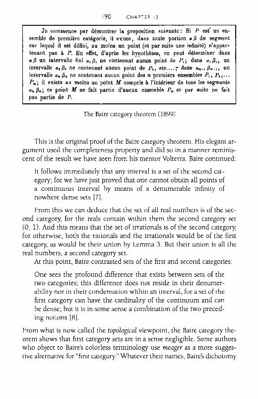
190 CHAPTER 13

Je commence par demontrer la proposition suivante: Si l' est" un en­semble de premiere categorie, il existe, dans toute portion tX p du segmentsur lequel il est defini, au moins un point (Elt par suite une i-nfinite) n'appar­tenant pas a P. En effet, d'apres les hypotheses, on peut determiner danstX (j un intervalle fini tX, P, ne contenant aucun point de 1', j dans tX, p" unintervalle tX. {3. ne contenant aucun point de 1'., etc.... j dans tXn-, {3n-" unintervalle tXn (jn ne contenant aucun point des 11 premiers ensembles 1'" 1'., ...Pn j i1 existe au moins un point M compris a I'interieur de tous les segmentstXn (jnj ce point M ne fait partie d'aucun ensemble Pn et par suite ne faitpas partie de p.

The Baire category theorem (1899)

This is the original proof of the Baire category theorem. His elegant ar­gument used the completeness property and did so in a manner reminis­cent of the result we have seen from his mentor Volterra. Baire continued:

It follows immediately that any interval is a set of the second cat­egory; for we have just proved that one cannot obtain all points ofa continuous interval by means of a denumerable infinity ofnowhere dense sets [7].

From this we can deduce that the set of all real numbers is of the sec­ond category, for the reals contain WIthin them the second category set(0, 1). And this means that the set of irrationals is of the second category,for otherwise, both the rationals and the irrationals would be of the firstcategory, as would be their union by Lemma 3. But their union is all thereal numbers, a second category set.

At this point, Baire contrasted sets of the first and second categories:

One sees the profound difference that exists between sets of thetwo categories; this difference does not reside in their denumer­ability nor in their condensation within an interval, for a set of thefirst category can have the cardinality of the continuum and canbe dense; but it is in some sense a combination of the two preced­ing notions [8].

From what is now called the topological viewpoint, the Baire category the­orem shows that first category sets are in a sense negligible. Some authorswho object to Baire's colorless terminology use meager as a more sugges­tive alternative for "first category." Whatever their names, Baire's dichotomy

BAIRE [91

would have important consequences for mathematical analysis, as the nextsection illustrates.

SOME ApPLICATIONS

A hallmark of mathematical progress is the fruitful generalization, onethat gathers seemingly unrelated matters under a single umbrella. Such ageneralization is both more efficient and more elegant than what came be­fore. The Baire category theorem is one of these, as is clear if we return toCantors nondenumerability result from chapter 11.

Cantor's Theorem Revisited: If {xh} is a sequence of distinct real num­bers, then any open interval (a, {3) contains a point not includedamong the {xh}'

Proof: The collection {Xl' X 2 , X 3 , ... , Xk, ... J, considered as a set of points,is denumerable and thus of the first category. Because Baire showedthat a first category set cannot exhaust an open interval, (a, {3) mustcontain a point other than the {xh}' Q.E.D.

That was certainly easy.But there is more. Volterras major result from chapter 12 is also a con­

sequence of Baires work. To see this, we need some background, includ­ing an immediate corollary of the category theorem.

Corollary: The complement of a first category set is dense.

Proof: (Recall that the complement of a set of real numbers A, often de­noted by N, is the set of real numbers not belonging to A.) Let F beof the first category and consider any open interval (a, {3). Baire provedthat not every point in (a, {3) belongs to F, so (a, {3) n fC"* 0, andthis is precisely what it required to show that the complement of F isdense. Q.E.D.

We next WIsh to characterize pointwise discontinuous functions interms of category, a quest that had led Baire to investigate category in thefirst place. In what follows, we join Baire in adopting the "inclusive"meaning of pointwise discontinuity, that is, continuity on a dense set. But

192 CHAPTER 13

our discussion differs from his original in that he employed the function'soscillation, whereas we reach the same end by means of sequences [9].

Beginning with a function f and a whole number k, we define the set

Ph == {xI there is a sequence aJ

---7 x withlf(aJ

) - f(x)l~ ~ for all J ~ I}0)

A real number x thus belongs to Ph if we can approach x sequentially bymeans of {a) in such a way that the functional values f( a)) and f(x) are allseparated by a gap of at least 11k. As an example, we again consider thefunction

sex) ={coso/x) if x :I; 0,o if x = 0

from chapter 10 and claim that 0 belongs to the set P2. To verify this, we

introduce the sequence {21

.}. Clearly lim _1_. = 0, and for each j ~ 11rJ J~OO 21rJ

we have 5 (2~j) -5(0) = lcos(21rj) - 01 = 1 ~ 1· By the definition in 0),

we see that 0 E P2 .

We are now ready to prove Baire's characterization of pointwise dis­continuity in terms of the "smallness" of Of'

Theorem: f is (at worst) pointwise discontinuous if and only if Of is a setof the first category.

There are, of course, two implications to be proved. We begin WIth themore intricate necessary condition.

Necessity: Iff is (at worst) pointwise discontinuous, then Of is of the firstcategory.

Proof: Our first object is to show that each Ph as defined above is nowheredense. We thus fix a whole number k ~ 1 and an open interval (a, 13). Bypointwise discontinuity,f is continuous at some point--call it xo-within

BAIRE 193

(a, [3). This means that lim f(x) = f(xo), and so, for £ =~, thereX---7Xo 3k

exists a 8> 0 such that the open interval (xo - 8, Xo + 8) is a subset of(a, [3) and

1if Ix - xol < 8, then If(x) - f(xo)1 <-.

3k(2)

We assert that (xo - 8, Xo+ 8) n Ph =0. To prove this, supposethe opposite. Then there is some point z belonging to (xo - 8,Xo + 8) n Ph. By the nature of Ph there must be a sequence aj ~ z

1with If(a J ) - fez) I~ k for all j ~ 1. Because the sequence {a) con-

verges to z E (xo - 8, Xo+ 8), there exists a subscnpt N so that aN E

(xo - 8, Xo+ 8). With some help from the triangle inequality, we con­clude that

1k~lf(aN)- f(z)I=lf(a N)- f(x o)+ f(x o)- f(z)1

1 1 2~lf(aN)- f(xo)I+lf(xo)- f(z)l< 3k + 3k = 3k'

where the last step follows from (2) and the fact that both IaN - Xo I< 8and Iz - xol < 8. This chain of inequalities leaves us with the contra-

1 2diction that - < -. Something is amiss.

k 3kThe trouble arose from the assumption that (xo - 8, Xo + 8) n Ph

is nonempty. We conclude instead that (xo - 8, Xo + 8) is a subintervalof (a, [3) that contains no points of Ph. By definition Ph is nowheredense for each k, and this in tum means that PI U P2 U ... U Ph U ...

is a set of the first category.We are nearly done. We need only apply the notion of continuity­

or, more precisely, of discontinuity-to see that

(3)

Expression (3) follows because if x E Df is any point of discontinuityoff, then there exists an £ > 0 so that, for any 8> 0, we can find a pointZ with 0 < Iz - xl < 8 yet If (z) - f (x) I ~ £. We then choose a whole

111number k with -k < £ and let 8 equal, in turn, 1, - ,-, ... to generate

2 3

194 CHAPTER [3

1points aI, a2 , a3 , . .. , aj , . .. with 0 < la} - xl <-:- but Ij(a) - j(x)1

)1

~ E > k' The sequence {a) converges to x, yet for all j ~ 1, we have

1Ij(a}) - j(x) I > k' By the definition in (1), the discontinuity point x be-

longs to the nowhere-dense set Ph and so, indeed, DJ~ P j U P2 U, .. U

Phu·· '.We wrap up this half of the proof by noting that DJ, a subset of the

first category set PI U P 2 U ... U Ph U .. " is itself first category bylemma 3. Therefore, if j is pointwise discontinuous, then Dr is a set ofthe first category. .

Sufficiency: If DJ is of the first category, then j is (at worst) pointwise dis­continuous.

Proof: This is an immediate consequence of the corollary to the Bairecategory theorem that we introduced earlier. Because DJ is of the first

category, its complement is dense. In other words, Dj =CJ = {x Ijis continuous at xl is dense, which is precisely what is required for j to

be at worst pointwise discontinuous. Q.E.D.

Thus the pointwise discontinuous functions are those whose assem­bled discontinuities remain "small" in the sense of being of the first cate­gory. This characterization reduced Hankel's thirty-year-old notion ofpointwise discontinuity to a simple condition on the set Dr Besides havingits own intrinsic value, it allowed Baire to give an elegant proof ofVolterra's theorem from the previous chapter [10].

Volterra's Theorem Revisited: There do not exist two pointwise dis­continuous functions on the interval (a, b) for which the continuitypoints of one are the discontinuity points of the other, and viceversa.

Proof: Suppose for the sake of argument that j and ¢ were two such func­tions. The previous theorem shows that both DJ and D1> are of the firstcategory and so too is DJ U D1> by lemma 4. By the Baire category the­orem, the complement of this union is dense. But the complement inquestion is the set of points at which neither function is discontinuous,

BAIRE 195

that is, the set of their common points of continuity. We have reacheda contradiction, for1and I/J share not just a single point of continuitybut a dense set of them. Q.E.D.

And, with little additional effort, Baire provided the folloWlng dra­matic extension [11 J.

Theorem: If 11,12, ... ,Ik' ... is a sequence of (at worst) pointwise dis­continuous functions defined on a common interval, then there is apoint-indeed, a dense set of points-at which all of these are simul­taneously continuous

Proof: As in the preceding proof, we consider Dfk , the set of discontinuitypoints of the function Ik' By pointwise discontinuity, each of these is ofthe first category, and so their union Df I U Df 2 U ... U Df k U ... is ofthe first category by Lemma 5. Again, the complement of this union isdense, but this complement is Cf I (1 Cf 2 (1 ... (1 Cf k (1 ... the pointswhere all the functions are continuous at once. Q.E.D.

This theorem shows that even though pointwise discontinuous func­tions can have infinitely many discontinuities, and even though we assem­ble a denumerable infinitude of such functions, enough continuity remainsto guarantee that they share a dense set of points where all are continuous.This represents a perfect fusion of set theory and analysis, blended togetherunder the watchful eye of Rene Baire.

Before leaving this section, we mention a last consequence Baire drewfrom his great theorem, one that led him to another lasting innovation[12].

Theorem: The uniform limit of pointwise discontinuous functions ispointWlse discontinuous.

Here he began with a sequence 11,12, ... ,Ik, ... of pointwise discon­tinuous functions defined on a common interval and assumed they con­verged uniformly to a function1 As we have seen, uniform convergence asdescribed by Weierstrass was sufficiently strong to transfer certain proper­ties from individual functions to their limit. Baire established that "point­Wlse discontinuity" was one such property.

Although omitting details, we give a sense of his argument. Underuniform convergence, Baire showed that any common point of continuity

196 CHAPTER 13

of the individual functions fh must be a point of continuity of the limitfunction f. To put this in set-theoretic notation, he proved

As we just saw, Baire knew that this denumerable intersection was dense,and so Cf must be dense as well. Then the uniform l,imit f, being continu­ous on a dense set, was pointwise discontinuous as claimed.

The fact that uniform limits of pointwise discontinuous functions mustbe pointwise discontinuous led Baire to wonder what, if anything, could besaid about nonuniform limits. His reflections produced a new taxonomy offunctions, much more sophisticated than Hankel's from a quarter-centuryearlier. We end the chapter with a discussion of these ideas.

THE BAIRE CLASSIFICATION OF FUNCTIONS

In the hope of categorizing functions into logically meaningful classes,Baire, like Hankel, took the continuous ones as his starting point. "I chooseto say that the continuous functions constitute class 0," he wrote, in theprocess solidifying his reputation for colorless terminology [13].

Suppose we have a sequence of continuous, that is, class 0, functionslfh}, and let f (x) = lim fh (x) be their pointwise limit. As we saw, f mayor

h~~

may not be continuous. In the latter case, the limit function has escapedfrom class 0, so Baire was ready with a new class. "Those discontinuousfunctions that are limits of continuous functions," he wrote, "form class 1."As an example, we recall from chapter 9 that each function fh (x) = (sin X)his continuous on [0, n], but f(x) = lim fh(X) is discontinuous at n12. So,

h~~f belongs to class 1.Baire proved something far more interesting: that functions in class 1

are at worst pointwise discontinuous [14]. That is, when we take a limit ofcontinuous functions, the outcome need not be continuous everywherebut must at least be continuous on a dense set. Taking limits of continu­ous functions, then, cannot obliterate all vestiges of continuity. On thecontrary, such limits retain a "respectable" amount of continuity from theoriginals. For those seeking a permanence in analysis, there is some com­fort in that conclusion.

One consequence is the following.

Theorem: Iff is differentiable, then its derivative l' must be continuouson a dense set.

BAIRE 197

f(x + 11k) - f(x)Proof: For each k ~ 1, we define a function fk (x) = k . The

IIdifferentiability off implies its continuity, so each fk is continuous as

well. But lim fk(X) = lim f(x + 11k) - f(x) = rex) because 11k ---7 0k~~ k~~ 11k

as k ---7 00. Hence l' is the pointwise limit of a sequence of functionsfrom class 0 and thus belongs to class 0 (in which case it is continu­ous) or to class 1 (in which case it is pointwise discontinuous). Eitherway, derivatives must be continuous on a dense set. Q.E.D.

We have previously seen that a differentiable function may have a dis­continuous derivative, but we can now answer the big question, "Howdiscontinuous can a derivative really be?" Thanks to Baire, the answer is,"Not very, for it must be continuous on a dense set."

Meanwhile, he continued his classification scheme:

Now suppose one has a sequence of functions belonging toclasses 0 or 1 and haVIng a limit function not belonging to eitherof these two classes. I will say that this limit function is of the sec­ond class, and the set of all functions that can be obtained in thismanner will form class 2 [15 l-

To establish that there is something in class 2, we define a function

D(x) = limrlim(COSk!JrX)2;]k~~;~~

and claim that, all appearances to the contrary, this is nothing but Dirich­let's function,

d(x) ={I ~f x ~s rational,o If x IS IrratIOnal.

We should take a moment to verify this claim. Note first that if x =plqis a ra~onal in lowest terms, then for any k ~ q, the expression k! JrX =k! Jr ( ~) is an integer multiple of Jr. Thus, for each k after a certain point,

lim(cosk! JrX)2; = lim(±l)2; = 1, and so D(x) = lim r lim(cos k! JrX)2;] = 1i~~ 1~~ k~~;~~

as well. On the other hand, if x is irrational, then k!Jrx cannot be an integermultiple of Jr, and it follows that leas k!Jrxl < 1. Consequently, for each k,

[98 CHAPTER 13

lim(cosk!Jrx)2 j = 0 and so D(x) = limflim(COSk!JrX)2J] = limO = O.J-too k-t~J-too k-too

Because D equals 1 at each rational and 0 at each irrational, it is indeedDirichlet's function traveling incognito.

What makes this intriguing is the analytic nature of D. When it wasintroduced early in the nineteenth century, Dirichlet5 function seemed sopathological as to lie beyond the frontier of analysis. Yet here we see it asnothing worse than the double limit of some well-behaved cosines.

Moreover, for each k andj, the function (cos k!JrX)2j is continuous, soDirichlet's function is seen to be the pointwise limit of the pointwise limitsof continuous functions. This places it in class 0, class 1, or class 2. But weknow that d is discontinuous everywhere and so does not belong to classo(which requires continuity) nor to class 1 (which requires continuity ona dense set). The only alternative is that Dirichlet's function resides inBaire's second class.

Baire was Just getting warmed up. A function that is the pointwiselimit of those from classes 0, 1, and 2 but does not belong to any of theseclasses is said to be in class 3. A limit of functions from classes 0, 1,2, or3 that escapes these will be in class 4. And on it goes. In the end we havean unimaginably vast tower of functions, beginning with continuous onesand evolving VIa repeated limits into ever more peculiar entities.

Needless to say, Baire's classification raised a host of questions. For in­stance, how can we be sure there are any functions in class 2477 And arethere functions so bizarre as to belong to no Baire class at alP It was Baire'scontemporary, Henri Lebesgue, who proved that the answer to both ofthese questions is a resounding "yes" [16].

Although ill health brought his career to an abrupt end, Rene Bairecarved out a share of mathematical immortality He introduced the di­chotomy between first and second category sets, proved and exploited hispowerful category theorem, and provided a classification of functions thatseemed to extend the boundaries of analysis to the far horizon.

As historian Thomas Hawkins observed, Baire's remarkable discover­ies showed that, even at the threshold of the twentieth century, the calcu­lus was still generating wonderful new problems [17]. In this regard,Lebesgue wrote of Baire's "rich imagination and solid critical sense" andcontinued,

Baire showed us how to investigate these matters; which problemsto pose, which notions to introduce He taught us to consider theworld of functions and to discern there the true analogies, the

BAIRE [99

genuine differences. In absorbing the observations that Baire made,one becomes a keen observer, learning to analyse commonplaceideas and to reduce them to notions more hidden, more subtle, butalso more effective.

In the end, Lebesgue called Baire "a mathematician of the highest class,"an impressive testimonial from one great analyst to another [18].

We conclude by returning to the chapter's opening passage: "Anyproblem relative to the theory of functions leads to certain questions rela­tive to the theory of sets." As we have seen, Baire lived by this motto. In­sofar as modern analysis has embraced his position, he deserves a largedebt of gratitude.

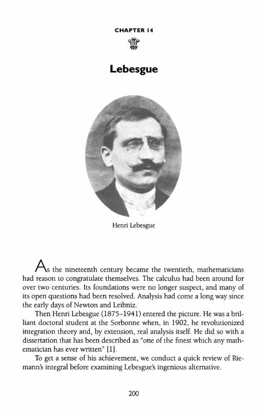
CHAPTER 14

Lebesgue

Henri Lebesgue

As the nineteenth century became the twentieth, mathematicianshad reason to congratulate themselves. The calculus had been around forover two centuries. Its foundations were no longer suspect, and many ofits open questions had been resolved. Analysis had come a long way sincethe early days of Newton and Leibniz.

Then Henri Lebesgue 0875-1941) entered the picture. He was a bril­liant doctoral student at the Sorbonne when, in 1902, he revolutionizedintegration theory and, by extension, real analysis itself. He did so with adissertation that has been described as "one of the finest which any math­ematician has ever written" Ill.

To gel a sense of his achievement, we conduct a quick review of Rie­mann's integral before examining Lebesgue's ingenious alternative.

200

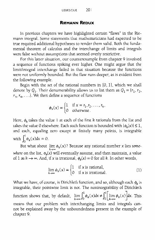
(1)

LEBESGUE 201

RIEMANN REOUX

In previous chapters we have highlighted certain "flaws" in the Rie­mann integral. Some statements that mathematicians had expected to betrue required additional hypotheses to render them valid. Both the funda­mental theorem of calculus and the interchange of limits and integralswere false WIthout assumptions that seemed overly restrictive.

For this latter situation, our counterexample from chapter 9 involveda sequence of functions spiking ever higher. One might argue that thelimit/integral interchange failed in that situation because the functionswere not uniformly bounded. But the flaw runs deeper, as is evident fromthe following example.

Begin with the set of the rational numbers in [0, I], which we shalldenote by Ql' Their denumerability allows us to list them as Q1 ={fl' f 2,

f 3 , f 4 , ... j. We then define a sequence of functions

Here, (h takes the value I at each of the first k rationals from the list andtakes the value 0 elsewhere. Each such function is bounded with !(Mx)1 ~ 1,and each, equaling zero except at finitely many points, is integrable

with f~ <l>k(x)dx = O.

But what about lim <l>k (x)? Because any rational number x lies some-k~oo

where on the list, <l>k(X) will eventually assume, and then maintain, a valueof 1 as k~ 00. And, if x is irrational, <l>k(x) =0 for all k. In other words,

lim <I> ( ) ={1 if x is rational,k~oo k X 0 if x is irrational.

What we have, of course, is Dirichlet's function, and so, although each <l>h isintegrable, their pointwise limit is not. The nonintegrability of Dirichlet's

function shows that, by default, lim rl<l>h(X)dxt=rl[lim<l>k(x)]dx. Thisk~oo Jo Jo k~oo

means that our problem with interchanging limits and integrals can­not be explained away by the unboundedness present in the example ofchapter 9.

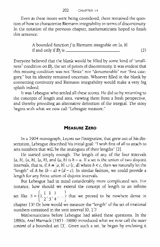
202 CHAPTER [4

Even as these issues were being considered, there remained the ques­tion of how to characterize Riemann integrability in terms of discontinuityIn the notation of the preVIous chapter, mathematicians hoped to finishthis sentence:

A bounded function f is Riemann integrable on [a, b]if and only if Df is (2)

Everyone believed that the blank would be filled by some kind of "small­ness" condition on Dr' the set of points of discontinuity It was eVIdent thatthis missing condition was not "finite" nor "denumerable" nor "first cate­gory," but its identity remained uncertain. Whoever filled in the blank byconnecting continuity and Riemann integrability would make a very bigsplash indeed.

It was Lebesgue who settled all these scores. He did so by returning tothe concepts of length and area, viewing them from a fresh perspective,and thereby proVIding an alternative definition of the integral. The storybegins WIth what we now call "Lebesgue measure."

MEASURE ZERO

In a 1904 monograph, Le(ons sur l'integration, that grew out of his dis­sertation, Lebesgue described his initial goal: "I WIsh first of all to attach tosets numbers that will be the analogues of their lengths" [2].

He started simply enough. The length of any of the four intervals[a, bJ, Ca, bJ, [a, b), and Ca, b) is b - a. If a set is the union of two diSjointintervals, that is, if A = [a, b] u [C, dl where b < c, then we naturally let the"length" of A be Cb - a) + Cd - c). In similar fashion, we could provide alength for any finite union of disjoint intervals.

But Lebesgue had in mind considerably more complicated sets. Forinstance, how should we extend the concept of length to an infinite

{II I }set like 5 = I, - , - ,-, . .. that we proved to be nowhere dense in234

chapter 137 Or how would we measure the "length" of the set of irrationalnumbers contained in the unit interval [0, IF

Mathematicians before Lebesgue had asked these questions. In the1880s, Axel Harnack (1851-1888) introduced what we now call the outercontent of a bounded set [3]. Given such a set, he began by enclosing it

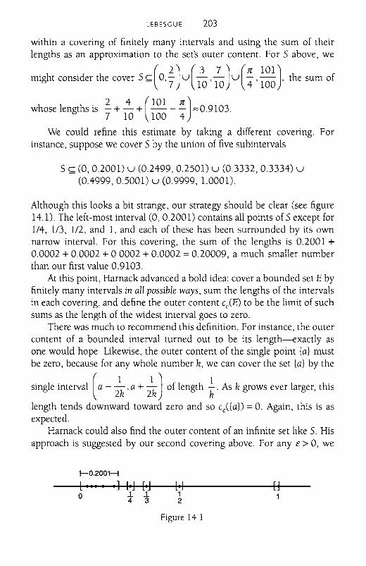
LEBESGUE 203

within a covering of finitely many intervals and using the sum of theirlengths as an approximation to the set's outer content. For 5 above, we

might consider the cover 5 k ( 0, f) u (130 ' 1

70) u ( ~, ~~~Jthe sum of

2 4 (101 TC)whose lengths is - + - + - - - ""0.9103.7 10 100 4

We could refine this estimate by taking a different covering. Forinstance, suppose we cover 5 by the union of five subintervals

S k (0, 0.2001) u (0.2499, 0.2501) u (0.3332, 0.3334) u(0.4999,0.5000 u (0.9999, 1.0001).

Although this looks a bit strange, our strategy should be clear (see figure14.1). The left-most interval (0, 0.2001) contains all points of 5 except for1/4, 1/3, 1/2, and 1, and each of these has been surrounded by its ownnarrow interval. For this covering, the sum of the lengths is 0.2001 +0.0002 + 0.0002 + 00002 + 0.0002 =0.20009, a much smaller numberthan our first value 0.9103.

At this point, Harnack advanced a bold idea: cover a bounded set E byfinitely many intervals in all possible ways, sum the lengths of the intervalsin each covering, and define the outer content c/E) to be the limit of suchsums as the length of the widest interval goes to zero.

There was much to recommend this definition. For instance, the outercontent of a bounded interval turned out to be its length-exactly asone would hope Likewise, the outer content of the Single point {a} mustbe zero, because for any whole number k, we can cover the set {a} by the

Single interval (a - 21k 'a+ 2

1k) of length t. As k grows ever larger, this

length tends downward toward zero and so c/{al) = O. Again, this is asexpected.

Harnack could also find the outer content of an infinite set like S. Hisapproach is suggested by our second covering above. For any E> 0, we

f-O.2001--;

[ ....o

0] [oJ [0]1. 1.4 3

Figure 14 1

204 CHAPTER 14

note that the interval ( 0, ~) contains all but finitely many points of 5,

which we denote by ~ _1_ ~, and 1. We then include each ofN'N-1'···'2

t:these N points in a tiny interval of width For example, we could

4N

place ~ within (~ - ~ , ~ +~) .Together these intervals cover 5, andk k 8Nk 8N

the sum of their lengths is

Because, for each t: > 0, 5 lies within finitely many intervals of total lengthless than t:, we conclude that ceCS) =o. We have here an infinite, nowhere­dense set of zero outer content.

But Harnack confronted a different situation with the set Q] of ratio­nals in [0, 1]: an infinite, dense set. He recognized that any covenng of Q]by a finite number of intervals will of necessity cover all of [0, 1]. HenceceCQ]) = 1. That is, the outer content of all rationals in the unit interval isthe same as the outer content of the unit interval itself.

In some ways, this seemed to make sense, but in others it appearedproblematic. For if we let I] be the set of irrationals in [0, 1], identical rea­soning shows that ceCIl) = 1 as well. Because the union of the diSjoint setsQ] and I] is the entire interval [0, 1], we see that

Apparently, we cannot decompose a set into disjoint subsets and sum theirouter contents to get the outer content of the original. Such nonadditivitywas an unwelcome feature of Harnack's theory of content.

The promise of extending the concept of length to nonintervals wassufficient to lead others to modify the definition so as to eliminate theattendant problems. Many mathematicians contributed to this discussion,but history credits Lebesgue with its final resolution. He defined a set tobe of measure zero if it "can be enclosed in a finite or a denumerable infini­tude of intervals whose total length is as small as we wish" [4]. Thus a set

LEBESGUE 205

E is of measure zero, written m(E) =0, if for any E> 0, we can enclose

E~ (aI' bl ) U (a2 , b2) U ... u (ak , bk) U ... , where L (bk - ak ) < E. Thek=l

innovation here is that Lebesgue, unlike Harnack, permitted coverings by adenumerable infinitude of intervals, and this made a world of difference.

It is obVIous from the definitions that any subset of a set of measurezero must itself be of measure zero. It is equally clear that a set with outercontent zero has measure zero as well. Thus, single points and the set 5above are of measure zero. But the converse fails-and fails spectacularly­as Lebesgue showed when he proved the follOwing.

Theorem: If a set E =EI U E2 U ... U Ek U . .. is the denumerableunion of sets of measure zero, then E is a set of measure zero also [5].

Proof: Let E> ° be given. By hypothesis, we can enclose EI in adenumerable collection of intervals of combined length less than

!:.- we can enclose E2 in a denumerable collection of intervals of4

Ecombined length less than -, and in general we enclose Ek in a

8

denumerable collection of intervals of length less than _E_ The given2 k+l

set E is then a subset of the union of all these intervals which, being thedenumerable union of denumerable collections, is itself a denumer-

able collection whose combined length is less than !:.- + !:.- + ... +4 8

E E2 k+l + ... = "2 < E. Because E has been enclosed in a denumerable

collection of intervals haVIng combined length less than the arbitrarilysmall number E, we see that E has measure zero. Q.E D.

It follows that any denumerable set is of measure zero, for such a setcan be written as the (denumerable) union of its individual points.In particular, the set of rational numbers in [0, l]-the dense set labeledQr above-has measure zero. Because m(QI) = °but ce(Qr) = 1, it isevident that zero outer content and zero measure are fundamentallydifferent.

A lesser mathematician might have retreated before the phenomenonof a dense set with measure zero. Dense sets, after all, were ubiquitous

206 CHAPTER 14

enough to be present in any interval no matter how tiny. Harnack himselfhad started down this path twenty years earlier but had rejected the ideaas being ridiculous [6]. Such a prospect seemed suffiCiently paradoxical toconvince him to stick with finite coverings.

But Lebesgue was not deterred, and his approach proved its worthwhen he found the long-sought relationship between a function's integra­bility and its points of continuity. "How discontinuous can an integrablefunction be?" was the question. Here is the simple answer.

Theorem: For a bounded function f to be Riemann integrable on [a, b], itis necessary and sufficient that the set of its points of discontinuity beof measure zero [7].

That is, he filled the critical blank in (2) with the condition m(Dr) =O. Inmany books, this is called "Lebesgue's theorem," indicating that, amongthe large number of results he eventually proved, this one was especiallysignificant

At the heart of Lebesgue's argument, not surprisingly, lay the Riemannintegrability condition, which can be recast as: f is Riemann integrableif and only if, for any E> 0 and any a> 0, we can partition [a, b] intofinitely many subintervals in such a way that those containing pointswhere the oscillation of the function is greater than a (what we called theType A subintervals) have combined length less than E

We observe that by the time of Lebesgue, the notion of a function's"oscillation" at a point had been made more precise than in Riemann's day.For our purposes, we shall continue to think of it informally as the maxi­mum variability of the function in the vicinity of the point. In addition, itwas known that a function is continuous at Xo if and only if its oscillationat Xo is zero.

Lebesgue introduced Gj(a) as the set of points in [a, b] where thefunction's oscillation is greater than or equal to a and showed that G j (a)

is a closed, bounded set. Because Cr= {x Ithe oscillation at x is zero}, weknow that .

Df = {x Ithe oscillation at x is greater than zero}

= Gj (1) U Gj [ ±)U ... U Gj[i) U ... (3)

LEBESGUE 207

The validity of equation (3) should be clear. On the one hand, at any point1

of discontinuity, the oscillation must be positive and hence exceed - forN

some whole number N. This means the discontinuity point belongs to

G{~ ) and consequently to the union on the right side of (3). Conversely,

any point in this union must belong to some G{~ ) and thus has a positive

oscillation, making it a discontinuity point.With this background, we consider Lebesgue's argument.

Proof: First, assume the bounded function f is Riemann integrable on[a, b]. For any whole number k, the integrability condition guarantees

that the set of points where the oscillation is greater than _1_ can bek+1

enclosed in finitely many intervals whose combined length is as small

as we wish. Thus this set, as well as its subset G{tl has zero content,

and so GI ( t) has measure zero. By theorem 1, the union

GI (1) U Gil~Ju ... u Gil~Ju ... will then be of measure zero,

which implies, by (3), that Dj is of measure zero also. This completesone direction of the proof.

For the converse, assume that m(Dj ) =0 and let both f> 0 and

a> O. Choose a whole number k with..!. < a. Then the set of pointsk

where the oscillation exceeds a is a subset of G{tl which, in turn,

is a subset of Dr Hence, G{~) is of measure zero and so can be

enclosed in a denumerable collection of (open) intervals of total length

less than f. Because G{i) is closed and bounded, Lebesgue could

208 CHAPTER 14

apply the famous Heine-Borel theorem to conclude that G{~)

lay within a finite subcollection of these open intervals [8]. This finitesubcollection obviously has total length less than E and covers not

only G{~) but the smaller set of points where the oscillation exceeds

CJ. In short, the integrability condition is satisfied and f is Riemannintegrable. Q.E.D.

Later, Lebesgue defined a property to hold almost everywhere if the setof points where the property fails to hold is of measure zero. With this ter­minology, we rephrase Lebesgue's theorem succinctly as follows: A bound­ed function on [a, b] is Riemann integrable if and only if it is continuousalmost everywhere.

We can use this characterization, for example, to give an instant proofof the integrability of the ruler function R on [0, I]. As we demonstrated,R is continuous except at the set of rational points whose measure is zero.This means that the ruler function is continuous almost everywhere andso is Riemann integrable. Case closed.

Lebesgue's theorem is a classic of mathematical analysis. In light ofwhat was to come, there is a certain irony in the fact that the person whofinally understood the Riemann integral was the one who would soon ren­der it obsolete: Henri Lebesgue.

THE MEASURE OF SETS

The notion of zero measure, for all of its importance, is applicableonly for certain sets on the real line. As he continued his thesis, Lebesguedefined "measure" for a much larger collection of sets. The basic idea wasborrowed from his countryman Emil Borel (1871-1956), but Lebesgueimproved upon it (dare we say?) immeasurably

The approach has a familiar ring. For a set E C [a, bl, Lebesgue wrote:

We can enclose its points within a finite or denumerably infinitenumber of intervals; the measure of the set of points of theseintervals is ... the sum of their lengths; this sum is an upperbound for the measure of E. The set of all such sums has a small­est limit me(E), the outer measure of E [9].

LEBESGUE 209

Symbolically, this amounts to

where we have employed the irifimum, or greatest lower bound, of the setin question. Again, the difference between outer measure and outer con­tent is that Lebesgue allowed for denumerably infinite coverings alongWIth the finite ones He observed at once that m/E) ~ ce(E), for takingmore coverings can only decrease their greatest lower bound.

Next, he looked at the complement of E in [a, b] which we wnte asfC = {x Ix E [a, b] but x e E}. With the definition above, he found theouter measure of fC and then defined the inner measure of E as m/E) =(b - a) - me(fC).

Rather than determine the inner measure of E by means of the outermeasure of its complement, a modern treatment is likely to "fill" the set Efrom within by finite or denumerably infinite unions of intervals and thentake the least upper bound, or supremum, of the sum of their lengths. That

is, m'(E) = sup{i (b k - ak) I(a l ,b l ) U (a 2 ,b2 ) U (a 3 ,b3 ) U' .. ~ E}. Fork=l

bounded sets, the two approaches are equivalent, but the second oneapplies equally well if E is unbounded.

At this point, Lebesgue showed that "the inner measure is never greaterthan the outer measure," that is, miCE) ~ m/E), and then stated the key def­inition: "Sets for which the inner and outer measures are equal are calledmeasurable and their measure is the common value of miCE) and me(E)" [10].

The family of measurable sets is truly immense. It includes any inter­val, any open set, any closed set, and any set of measure zero, along withthe set of rationals and the set of irrationals. In fact, for some time mathe­maticians were unable to find a set that was not measurable, that is, onefor which m,(E) < me(E). These were eventually constructed by means ofthe axiom of choice and turned out to be extremely complicated [11].

Lebesgue explored the consequences of his definitions, three of themost basic of which were:

1. If E is measurable, then m(E) ~ O.2. The measure of an interval is its length.

210 CHAPTER 14

3. If EI , E2 , ... , E", ... is a finite or denumerabIy infinite collec­tion of pairwise disjoint measurable sets and if E =EI U E2 U

... u E" u ... is their union, then E is measurable and m(E) =m(E I ) + m(E2) + ... + m(E,,) + ....

This third condition is the additivity property that outer content lacked.With it, we can easily find the measure of the set of irrationals in [0, 1],which we called II above. We note that [0,1] =QI u II' where the two setson the right are disjoint and measurable. Thus, 1 = m[O, 1] = m(QI u II) =

m(QI) + m(II) =0 + m(II), and so m(II) = 1. In terms of measure, the irra­tionals dominate [0, 1], whereas the rationals are insignificant.

Among other things, Lebesgue measure provided a new dichotomybetween "small" (measure zero) and "large" (positive measure). This tookits place alongside the cardinality dichotomy (denumerable versus nonde­numerable) and the topological one (first category versus second category).In all three, the rationals qualify as small for they are of measure zero,denumerable, and of the first category, whereas the irrationals are large(being of positive measure), nondenumerable, and of the second category.

To continue with this idea, we have seen that, for any of thesedichotomies, subsets and denumerable unions of "small" sets are "small,"and we have proved that a denumerable set is both of the first categoryand of measure zero. However, other "large/small" connections do nothold. It is possible to find first category sets that are nondenumerable andof positive measure and to find measure zero sets that are nondenumer­able and of the second category [12]. Obviously, these concepts had carriedmathematicians into some deep waters.

In his dissertation, Lebesgue was not content to consider just meas­urable sets. He defined a measurable junction in these words: "We say thata function j, bounded or not, is measurable if, for any ex < [3, the set{xl ex <j(x) < [3) is measurable" [13]. The diagram in figure 14.2 gives a geo­metric sense of this definition. For ex < [3 along the y-axis, we collect all pointsx in the domain whose functional values fall between ex and [3. If this set ismeasurable for all choices of ex and [3, we say that j is a measurable function.

Using properties of measurable sets, Lebesgue showed that j is a mea­surable function if and only if, for any ex, the set {xl ex <j(x)} is measurable.From this result it easily follows that Dirichlet's function d is measurable,because there are only three possibilities for the set {xl ex < d(x)}: it isempty if ex ~ 1; it is the set of rationals if 0 < ex ~ 1; and it is the set of allreal numbers if ex ~ O. In each case, these are measurable sets, so d is ameasurable function.

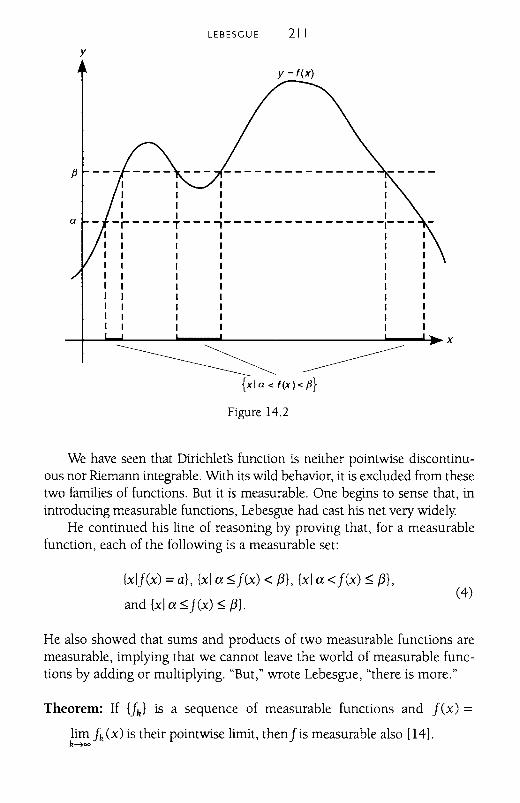
LEBESGUE 21 1y

Y =f(x)

fJ

a

III

I I I I- -r----T---'----------------r-- -I I I I II I I I II I I I II I I I II I I I II I I I II I I I II I I I II I I I II I I I I

_+--L....L. I.._...I. .1-_~~X

~~{xI a < f(x) < fJ}

Figure 14.2

We have seen that Dirichlets function is neither pointwise discontinu­ous nor Riemann integrable. With its wild behavior, it is excluded from thesetwo families of functions. But it is measurable. One begins to sense that, inintroducing measurable functions, Lebesgue had cast his net very widely

He continued his line of reasoning by proving that, for a measurablefunction, each of the following is a measurable set:

{xIJ(x) =a}, {xl ex ~J(x) < f3}, {xl ex <J(x) ~ f3},

and {xl ex ~J(x) ~ f3}.(4)

He also showed that sums and products of two measurable functions aremeasurable, implying that we cannot leave the world of measurable func­tions by adding or multiplying. "But," wrote Lebesgue, "there is more."

Theorem: If Uk} is a sequence of measurable functions and J(x) =

lim fk (x) is their pointwise limit, thenJis measurable also [14].k~oo

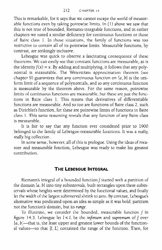
212 CHAPTER 14

This is remarkable, for it says that we cannot escape the world of measur­able functions even by taking pointwise limits. In (1) above we saw thatthis is not true of bounded, Riemann-integrable functions, and in earlierchapters we noted a similar deficiency for continuous functions or thoseof Baire class 1. In those situations, the family of functions was toorestrictive to contain all of its pointwise limits. Measurable functions, bycontrast, are strikingly inclusive.

Lebesgue was quick to observe a fascinating consequence of thesetheorems. We can easily see that constant functions are measurable, as isthe identity f(x) =x. By adding and multiplying, it follows that any poly­nomial is measurable. The Weierstrass approximation theorem (seechapter 9) guarantees that any continuous function on [a, b] is the uni­form limit of a sequence of polynomials, and so any continuous functionis measurable by the theorem above. For the same reason, pointwiselimits of continuous functions are measurable, but these are Just the func­tions in Baire class 1. This means that derivatives of differentiablefunctions are measurable. And so too are functions of Baire class 2, suchas Dirichlet's function, for these are pointwise limits of functions in Baireclass 1. This same reasoning reveals that any function of any Baire classis measurable.

It is fair to say that any function ever considered prior to 1900belonged to the family of Lebesgue-measurable functions. It was a really,really big collection.

In some sense, however, all of this is prologue. Using the ideas of mea­sure and measurable function, Lebesgue was ready to make his greatestcontribution.

THE LEBESGUE INTEGRAL

Riemann's integral of a bounded function f started WIth a partition ofthe domain [a, b] into tiny subintervals, built rectangles upon these subin­tervals whose heights were determined by the functional values, and finallylet the width of the largest subinterval shrink to zero. By contrast, Lebesgue'salternative was predicated upon an idea as simple as it was bold: partitionnot the function's domain, but its range.

To illustrate, we consider the bounded, measurable function f infigure 14.3. Lebesgue let 1< L be the infimum and supremum of f over[a, b]-that is, the least upper and greatest lower bounds of the function­al values-so that [I, L] contained the range of the function. Then, for

LEBESGUE 213

y

LY =f(x)

I I I I-- r----'---r-----------------II III III III III III III III III III III III III I

-.j--""""'!-------.....-----------------... x

~~Ek = {x leks f(x) < ek+d

Figure 14.3

any E> 0, Lebesgue imagined a partition of the interval [I, L] by means ofthe points

where the greatest gap between adjacent partition points was less than E.

With such a partition along the y-axis, we form the "Lebesgue sum."Like a Riemann sum, this will approximate the area under the curvewith regions of known dimensions, although we can no longer be certainthese regions are rectangular. Rather, we consider the subinterval [lh, Ih+l)

along the y-axis and look at the subset Eh of [a, b] defined by Eh ={x11h ~f(x) < Ih+ll. This is the portion of the x-axis indicated in figure14.3. Here, Eh is the union of three intervals, but its structure can be muchmore complicated depending on the function at hand.

At the analogous stage in Riemann's approach, we would construct arectangle whose height was an approximation of the function's value,

214 CHAPTER 14

whose width was the length of the appropriate subinterval, and whosearea was the product of these two. For Lebesgue, we use lk to approximatethe value of the function on the set Ek, but how do we determine "length"if Ek is not an interval?

The answer, which should come as no surprise, is to use the measureof the set Ek in this role. Upon multiplying height and "length," we getlk . meEk) as the counterpart of the area of one of Riemanns thin rectangles.We sum these over all subintervals of the range to get a Lebesgue sum,

n

L lk . m(Ek), where for the last term of this series we let En ={xIf (x) =In}'k=O

Finally, Lebesgue let e~ 0 so that the maximum value of lk+l - lkapproaches zero as well. Should this limiting process lead to a uniquevalue, we say that f is Lebesgue integrable over la, b] and define

We must address two issues before proceeding. First, it is clear thatthe sets Eo, E1, E2 , ... , En-I' En partition la, b] into subsets, althoughnot necessarily into subintervals. Second, our assumption that f is mea­surable implies, by (4), that each Ek = {xllk ~f(x) < lk+l} along withEn = {xlf(x) = In} is a measurable set, and so we may properly talk aboutmeEk)' Everything is falling nicely into place.

In a work written for a general audience, Lebesgue used an analogy tocontrast Riemann's approach and his own [15]. He imagined a shopkeep­er who, at day's end, wishes to total the receipts. One option is for themerchant to "count coins and bills at random in the order in which theycame to hand." Such a merchant, whom Lebesgue called "unsystematic,"would add the money in the sequence in which it was collected: a dollar,a dime, a quarter, another dollar, another dime, and so on. This is liketaking functional values as they are encountered while moving fromleft to right across the interval la, bl. With Riemann's integral, the processis "driven" by values in the domain, and values in the range fall wherethey may.

But, Lebesgue continued, would it not be preferable for the merchantto ignore the order in which the money arrived and instead group it bydenomination? For instance, it might turn out that there were in all a dozendimes, thirty quarters, fifty dollars, and so on. The calculation of the days

LEBESGUE 215

receipts would then be simple: multiply the value of the currency (whichcorresponds to the functional value lh) by the number of pieces (which cor­responds to the measure of Eh) and add them up. This time, as withLebesgue's integral, the process is driven by values in the range, and thesets Eh that subdivide the domain fall where they may.

Lebesgue conceded that for the finite quantities involved in running abusiness, the two approaches yield the same outcome. "But for us whomust add an infinite number of indivisibles," he wrote, "the differencebetween the two methods is of capital importance." He emphasized thisdifference by observing that

our constructive definition of the integral is quite analogous tothat of Riemann; but whereas Riemann divided into small subin­tervals the interval of variation of x, it is the interval of variation ofj(x) that we have subdivided [16].

To show that he was not chasing definitions pOintlessly, Lebesgueproved a number of theorems about his new integral. We shall consider afew of these, albeit without proof.

Theorem 1: Ifjis a bounded, Riemann-integrable function on [a, bl, then

j is Lebesgue integrable and the numerical value of J: j(x)dx is the

same in either case.

This is comforting, for it says that Lebesgue preserved the best of Rie­mann.

Theorem 2: If j is a bounded, measurable function on [a, bl, then itsLebesgue integral exists.

Here we see the power of Lebesgue's ideas, because the family ofmeasurable functions is far more encompassing than the family of Rie­mann integrable ones (i.e., those continuous almost everywhere). To putit Simply, Lebesgue could integrate more functions than Riemann. Theo­rems 1 and 2 show that Lebesgue had genuinely extended the previoustheory.

For example, we have seen that Dirichlets function is bounded and

measurable on [0, 1]. Consequently, J~ d(x)dx exists as a Lebesgue integral,

in spite of the fact that it is meaningless under Riemanns theory.

216 CHAPTER 14

Better yet, it is easy to calculate the value of this integral. We start withany partition of the range: 0 =10 < II < 12 < ... < 'n = 1. By the nature ofDirichlet's function,

Eo = {xiO ~ d(x) < 'll = II, the set of irrationals in [0, 1],

Ek = {x1lk ~ d(x) < 'k+Il = 0 for k = 1,2, ... , n - 1,

En = {xld(x) = l} = QI' the set of rationals in [0, 1].

For this arbitrary partition, the Lebesgue sum is

n

L Ik • meEk) = O· m(Eo) + 'I . m(EI) + ... + 'n-I· m(En_ I ) + 1 . m(En )

k=O

= O· m(II) + 'I . m(0) + ... + 'n-I· m(0) + 1 . m(QI)

= 0·1 + 'I ·0+· .. + 'n-I· 0 + 1· 0 = O.

And because the Lebesgue sum is zero for any partition, the limit of all

such is zero as well. That is, f: d(x)dx = O.

The fact that Dirichlet's function is everywhere discontinuous ren­dered it nonintegrable for Riemann, but such universal discontinuity wasof no consequence for Lebesgue. Here was indisputable mathematicalprogress.

Theorem 3: If j and g are bounded, measurable functions on [a, b] and

j (x) =g(x) almost everywhere, then f: j(x)dx = f: g(x)dx.

This result says that changing the values of a measurable function ona set of measure zero has no effect on the value of its Lebesgue integral.For Riemann, we can change the function's value at finitely many pointswithout altering the integral, but once we tamper with an infinitude ofpoints, all bets are off. By contrast, Lebesgue's integral is sufficientlytamper-proof that we can modify the function on an infinite set of zeromeasure yet leave the integral-and the integrability-intact.

To see this theorem in action, we revisit Dinchlet's function d and theruler function R on [0, 1] and form a trio by introducing g(x) =0 for all x

in [0, 1]. The three functions d, R, and g are certainly not identical, forthey differ at rational points in the unit interval. But such differences are

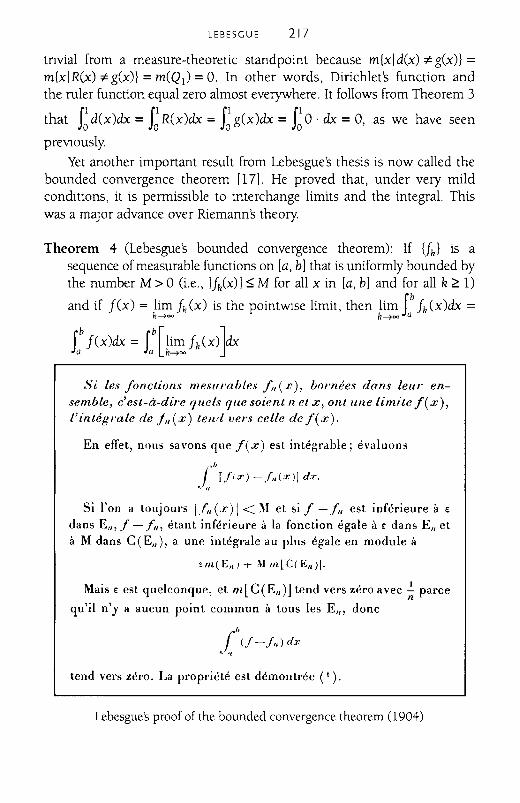
LEBESGUE 217

tnvial from a measure-theoretic standpoint because m{xld(x) :;tg(x)} =m{xIR(x) :;tg(x)} = m(Qj) = O. In other words, Dirichlet's function andthe ruler function equal zero almost everywhere. It follows from Theorem 3

that f~ d(x)dx = f~ R(x)dx = f~ g(x)dx = f~ 0 . dx =0, as we have seen

preVlously.

Yet another important result from Lebesgue's thesis is now called thebounded convergence theorem [17]. He proved that, under very mildconditions, it is permissible to interchange limits and the integral. Thiswas a major advance over Riemanns theory.

Theorem 4 (Lebesgues bounded convergence theorem): If Uk} is asequence of measurable functions on la, b] that is uniformly bounded bythe number M > 0 (i.e., Ifk(x) I~ M for all x in la, b] and for all k ~ 1)

and if f(x) = lim fk(X) is the pointWIse limit, then lim fb fk(X)dx =k--->= k--->= a

fb f(x)dx = fb[lim fk(X)]dxa a k--->=

Si les fonctions meslIl'ables f" (.£), bOl'nees dans leur en­semble, c'est-it-dire quels que soient n et x, ont llne limite I( x),l'integrale de ill (x) tell'{ vel's celie de f( x).

En eITet, nOlls sa vons que f( x) est integt'able; evaluons

j'b

f/(.T) - /,,(X)] d.r.

"Si l'on a toujours 1/" (.r) I< 'I et si f - f" est inferieure a €

dans E", f - f", etallt inferieure a la fonetion egale a € dans E" eta M dans C(E,,), a une integrale au plus egale en module it

sm( En} +- ;n m[ C( En)].

Mais € est queIeonque, et m[C(E,,» tend vers zero avee ~ pareen

qu'il n'y a aueun point eommun a tous les E'/l done

f'b

(j-/Il)dx., 'I

tend vers zero. La propriete est demontree (t ).

Lebesgue's proof of the bounded convergence theorem (904)

218 CHAPTER 14

We can use this to launch our third attack upon f~ d(x)dx. Earlier, we

introduced a sequence of functions {~k} on [0, 1] for which lim ~k(X) =k~=

d(x),as seen in (1). Clearly, I if>k(X) I :::; 1 for all x and all k, so this is a

uniformly bounded family, and because each ~k is zero except at k

points, we know that each function is measurable with f: if>k(x)dx = O. By

Lebesgue's bounded convergence theorem, we conclude yet again that

r1d(x)dx = r1

[lim if>k (x)]dxJo Jo h~=

= lim r1~h(x)dx = rIO. dx = o.

h~=JO Jo

There is time for one last flourish. We recall that Volterra had discov­ered a pathological function WIth a bounded, nonintegrable denvative. Ofcourse, in Volterra's day, "nonintegrable" meant "non-Riemann-integrable."

By adopting Lebesgue's alternative, however, the pathology disap­pears. For if F is differentiable with bounded derivative F', then the

Lebesgue integral f: F'(x)dx must exist because, as we saw in chapter 13,

F' belongs to Baire class 0 or Baire class 1. This is sufficient to make itLebesgue integrable.

Better yet, the bounded convergence theorem allowed Lebesgue toprove the folloWIng [18].

Theorem 5: If F is differentiable on [a, b] with bounded derivative, then

f:F'(x)dx =F(b) - F(a).

Here, back in all its original glory, is the fundamental theorem of cal­culus. With Lebesgue's integral, there was no longer the need to attachrestrictive conditions to the derivative, for example, a requirement that itbe continuous, in order for the fundamental theorem to hold. In a sense,then, Lebesgue restored this central result of calculus to a state as "natural"as it was in the era of Newton and Leibniz.

In closing, we acknowledge that many, many technicalities have beenglossed over in this brief introduction to Lebesgue's work. A completedevelopment of his ideas would require a significant investment of timeand space, which makes it all the more amazing that these ideas are taken

LEBESGUE 219

from his doctoral thesis! It is no wonder that the dissertation stands in aclass by itself.

We end with a final observation from Lebesgue. In the preface of hisgreat 1904 work, he conceded that his theorems carry us from "nice"functions into a more complicated realm, yet it is necessary to inhabit thisrealm in order to solve simply stated problems of historic interest. "It is forthe resolution of these problems," he wrote, "and not for the love of com­plications, that I introduce in this book a definition of the integral moregeneral than that of Riemann and containing it as a particular case" [19].

To resolve historic problems rather than to complicate life: a worthyprinciple that guided Henri Lebesgue on his mathematical journey.

Afterword

Our VIsit to the calculus gallery has come to an end.Along the way, we have considered thirteen mathematicians whose

careers fall into three separate periods or, at the risk of overdoing the anal­ogy, into three separate wings.

First came the Early Wing, which featured work of the creators, New­ton and Leibniz, as well as of their immediate followers: the BernoulliBrothers and Euler. From there we visited what might be called the Classi­cal Wing, WIth a large hall devoted to Cauchy and sizable rooms for Rie­mann, liOUVIlle, and Weierstrass, scholars who supplied the calculus withextraordinary mathematical rigor. Finally, we entered the Modern Wing ofCantor, Volterra, Baire, and Lebesgue, who fused the precision of the clas­sicists and the bold ideas of set theory.

Clearly, the calculus on display at tour's end was different from thatwith which it began. Mathematicians had gone from curves to functions,from geometry to algebra, and from intuition to cold, clear logic. Theresult was a subject far more sophisticated, and far more challenging, thanits originators could have anticipated.

Yet central ideas at the outset remained central ideas at the end. Asthe book unfolded, we witnessed a continuing conversation among thosemathematicians who refined the subject over two and a half centuries. Ina very real sense, these creators were addressing the same issues, albeitin increasingly more complicated ways. For instance, we saw Newtonexpand binomials into infinite series in 1669 and Cauchy provide con­vergence criteria for such series in 1827. We saw Euler calculate basicdifferentials in 1755 and Baire identify the continuity properties ofderivatives in 1899. And we saw Leibniz apply his transmutation theo­rem to find areas in 1691 and Lebesgue develop his beautiful theory ofthe integral in 1904. Mathematical echoes resounded from one era tothe next, and even as things changed, the fundamental issues of calculusremained.

Our book ended WIth Lebesgue's thesis, but no one should concludethat research in analysis ended there as well. On the contrary, his workrevitalized the subject, which has grown and developed over the past hun­dred years and remains a bulwark of mathematics up to the present dayThat story, and the new masters who emerged in the process, must remainfor another time.

220

AFTERWORD 221

We conclude as we began, with an observation from the great twenti­eth century mathematician John von Neumann. Because of achievementslike those we have seen, von Neumann regarded calculus as the epitomeof precise reasoning. His accolades, amply supported by the results of thisbook, will serve as the last word:

I think it [the calculus] defines more unequivocally than anythingelse the inception of modern mathematics, and the system ofmathematical analysis, which is its logical development, still con­stitutes the greatest technical advance in exact thinking. [1]

Notes

INTRODUCTION

1. John von Neumann, Collected Works, vol I, Pergamon Press, 1961, p 3.

CHAPTER INEWTON

1. Richard S Westfall, Never at Rest, Cambndge University Press, 1980, p. 134.

2 Ibid., P 202.3 Dirk Stroik (ed ), A Source Book in Mathematics, 1200-1800, Harvard University

Press, 1969, p. 2864 Ibid

5. Derek Whiteside (ed.), The Mathematical Works of Isaac Newton, vol I, Johnson

Repnnt Corp, 1964, p 376. Ibid., P 227 Ibid, P 208 Ibid, p. 39 Derek Whiteside (ed ), Mathematical Papers of Isaac Newton, vol. 2, Cambndge Uni-

versity Press, 1968, p 20610 WhiteSide, Mathematical Works, vol I, p 22.

11. Ibid., P 23.12. Ibid

13 Ibid., p. xiii.

14. Westfall, p. 205

15. Whiteside, Mathematical Works, vol. 1, p. 416 Ibid., p. 617 Ibid, pp 18-2118 Ibid, p. 20.

19. Whiteside (ed.), Mathematical Papers of Isaac Newton, vol. 2, p 237.20 DaVId Bressoud, "Was Calculus Invented in India7" The College Mathematics Jour­

nal, vol 33 (2002), pp. 2-1321 Victor Katz, A History of Mathematics: An Introduction, Harper-Collins, 1993,

pp 451-45322 C Gerhardt (ed ), Der Bnefwechsel von Gottfried Wilhelm Leibniz mit mathematik­

em, vol. I, Mayer &: Muller Berlin, 1899, p 170

223

224 NOTES

CHAPTER 2LEIBNIZ

1 Joseph E Hofmann, Leibniz in Pans 1672-1676, Cambridge University Press,

1974, pp 23-25 and p 79

2 See, for instance, Rupert Hall, Philosophers at War, Cambndge University Press, 1980

3 J M Child (trans ), The Early Mathematical Manuscnpts of Leibniz, Open Court Pub-

lishing Co , 1920, P 11

4 Ibid, P 12

5 Ibid

6 Struik, pp. 272-280, has an English translation

7 Robert E Montz (ed), Memorabilia Mathematica, MAA, 1914, P 323

8 Child, pp 22-58

9 Ibid, P 150

10 Struik, p 276

II Child, P 39

12 Ibid, P 42

13 Ibid, P 4614 Ibid, P 4715 Ranjan Roy, "The Discovery for the Series Formula for lC by Leibniz, Gregory and

Nilakantha," Mathematics Magazine, vol 63 (1990), no 5, pp 291-306

16 Child,p 46

CHAPTER 3THE BERNOULLIS

1 Howard Eves, An Introduction to the History of Mathematics, 5th Ed , Saunders Col­

lege Publishing, 1983, p 3222 Westfall, Never at Rest, pp 741-743

3 Morris Kline, Mathematical Thought from Ancient to Modern Times, Oxford Universi­

ty Press, 1972, p. 473.

4 Jakob Bernoulli, Ars conjectandi (Repnnt), Impression anastaltique, Culture et

CiVIlisation, Bruxelles, 19685 LHospital, Analyse des infiniment petits (Reprint), ACL-Editions, Paris, 1988, pp

145-146

6 Struik, p 3127 Dirk Struik, "The origin of I'Hospitals rule," Mathematics Teacher, vol 56 (1963),

P 2608 Johannis Bernoulli, Opera omnia, vol 3, Georg alms, Hildesheim, 1968, pp

385-563

9 The Tractatus is appended to Jakob Bernoulli's Ars conjectandi (cited above), pp

241-30610 See William Dunham,journey through Genius, Wiley, 1990, pp 202-205

NOTES 225

II Hofmann, p 3312 Jakob Bernoulli, Ars conjectandi, p 25013 Ibid, P 25114 Ibid, P 252IS Ibid, pp 246-24916 Ibid, P 25417 johannis Bernoulli, Opera omnia, vol I, Georg Olms, Hildesheim, 1968, p 18318 johannis Bernoulli, Opera omnia, vol 3, p 38819 Ibid,p 37620 johannis Bernoulli, Opera omnia, vol I, pp 184-18521 johannis Bernoulli, Opera omnia, vol 3, pp 376-38122 Ibid, P 38123 Ibid, P 377

CHAPTER 4EULER

Enc Temple Bell, Men of Mathematics, Simon & Schuster, 1937, P 1392 Leonhard Euler, Foundations of Differential Calculus, trans john Blanton, Springer-

Verlag, 20003 Ibid, P 514 Ibid, P 525 Ibid6 Ibid, P 1167 These integrals appear, respectively, in Leonhard Euler's, Opera omnia, ser I, vol

17,p 407,Operaomnia,ser I, vol 19,p 227,andOperaomnia,ser.l,vol 18,p 88 Euler, Opera omnia, ser I, vol 18, P 49 T L Heath, (ed ), The Works of Archimedes, Dover, 1953, p 9310 Howard Eves, An Introduction to the History of Mathematics, yh Ed , Saunders,

1983,p 86II Euler, Opera omnia, ser I, vol 16B, P 312 Ibid, pp 14-1613 Ibid, P 27714 Leonhard Euler, Introduction to Analysis of the Infinite, Book I, trans john Blanton,

Spnnge~Verlag, 1988,p 137IS Euler, Opera omnia, ser I, vol 6, pp 23-2516 Euler, Introduction to Analysis of the Infinite, Book I, pp 142-14617 Ivor Grattan-Guinness, The Development of the Foundations of Mathematical Analy-

sis from Euler to Riemann, MIT Press, 1970, p 7018 Euler, Opera omnia, ser I, vol 10, P 61619 Euler, Opera omnia, ser I, vol 4, P 14520 Philip Davis, "Leonhard Euler's Integral," Amencan Mathematical Monthly, vol 66

(1959), P 851

226 NOTES

21 P H Fuss (ed ), Correspondance mathematique et physique, The Sources of Science,No 35,johnson Repnnt Corp, 1968, p 3

22 Euler, Opera omnia, ser 1, vol 14, p 3.23 Ibid, P 1324 Euler, Opera omnia, ser. 1, vol I6A, p 154.25. Ibid., p. 15526. Euler, Opera omnia, ser. 1, vol 18, P 21727. john von Neumann, Collected Works, vol 1, Pergamon Press, 1961, p 5

CHAPTER SFIRST INTERLUDE

1. Stroik, p 3002. George Berkeley, The Works of George Berkeley, vol 4, Nelson &: Sons, London,

I95I,p 533 Ibid, P 674 Ibid., P 89.5 Ibid., p. 68.6 Ibid, p. 777 Ibid., P 728. Ibid., p. 73.9 Ibid., p. 7410 Carl Boyer, The Concepts of the Calculus, Hafner, 1949, p. 248.11. Stroik, p. 344.12 joseph-Louis Lagrange, Oeuvres, vol 9, Paris, 1813, p 11 (title page)13. Ibid, pp. 21-22.14 Augustin-Louis Cauchy, Oeuvres, ser 2, vol 2, Paris, pp 276-278.15. judith Grabiner, The Origms of Cauchy's Rigorous Calculus, MIT Press, 1981, p 3916 Berkeley, p. 76

CHAPTER 6CAUCHY

1. Bell, p. 292.2. The Cours d'analyse is available in Cauchys Oeuvres, ser. 2, vol. 3, and the Calcul

infinitesimal appears in the Oeuvres, ser. 2, vol. 43. Cauchy, Oeuvres, ser. 2, vol. 4, in the Advertisement of the Calcul infinitesimal.4 Ibid., p. 13.

5 Ibid, p. 16.6 Ibid, P 207. Ibid., P 198. Ibid., p. 23.9. Kline, p 947

NOTES 227

10 Cauchy, Oeuvres, ser 2, vol 3, pp. 378-380 Or see Judith Grabiner, The Ongms

of Cauchy's Rigorous Calculus, MIT Press, 1981, pp. 167-168 for an English translation.

11 Grabiner, p 69

12. Cauchy, Oeuvres, ser 2, vol 4, pp 44-46

13. Euler, Opera omnia, ser 1, vol 11, P 5

14 Cauchy's theory of the integral is taken from his Oeuvres, ser. 2, vol. 4, pp.122-127

15. Ibid, pp 151-155

16 Ibid, P 220

17 Ibid, pp 226-22718 Cauchy, Oeuvres, ser 2, vol 3, p 123

19 Ibid, P 137-13820 Boyer, p 271

CHAPTER 7RIEMANN

1 Euler, Introduction to Analysis of the Infinite, Book 1, pp 2-3

2 Euler, Foundations of Differential Calculus, p V1

3 Israel Kleiner, "Evolution of the Function Concept A Bnef Survey," College Mathe-maticsJournal, vol 20 (1989), pp 282-300

4 Thomas Hawkins, Lebesgue's Theory of Integration, Chelsea, 1975, pp 3-8

5 Ibid, pp 5-6

6 G Lejeune Dinchlet, Wake, vol 1, Georg RIemer Verlag, 1889, p. 120

7 Ibid., pp. 131-132

8. Hawkins, p. 169 Bernhard RIemann, Gesammelte Mathematlsche Wake, Spnnger-Verlag, 1990, p 271

10 Ibid

11 Ibid, P 27412 Ibid

13 Ibid, p. 270

14 Dirichlet, Wake, vol I, p 31815 RIemann, p 267

CHAPTER 8LIOUVILLE

1 Stroik, p 276

2 Euler, Introduction to Analysis of the Infinite, Book I, p 4

3 Ibid, P 804 Kline,pp 459-460

5 Ibid, P 593

228 NOTES

6 These and other aspects of Liouville's career are treated in jesper Lutzen's scientificbiography, Joseph Liouville 1809-1882' Master of Pure and Applied Mathematics, Springer­Verlag, 1990

7 E Hairer and G Wanner, Analysis by Its History, Spnnger-Verlag, 1996, p 1258, j LiouvJile, "Sur des classes tres-etendues de quantites don't la valeur n'est ni

algebnque, ni meme reductible a des irrationnelles algebriques," Journal de mathematiquespures et appliquees, vol 16 (1851), pp 133-142

9 This is adapted from George Simmons, Calculus Gems, McGraw-Hili, 1992, pp

288-28910 liouVIlle, Ibid1I Ibid, P 14012 Lutzen, pp 79-8113 Bell, p 46314 See, for instance, the discussion in Dunham, pp 24-2615 Andrei Shidlovskii, Transcendental Numbers, de Gruyter, 1989, p 442

CHAPTER 9WEIERSTRASS

1 This biographical sketch is drawn from the Weierstrass entry in the Dictionary ofScientific Biography, vol XlV, C C Gillispie, editor-in-chief, Scnbner, 1976, pp 219-224

2 Bell,p 4063 Hairer and Wanner, p 2154 Cauchys Oeuvres, ser 2, vol 3, P 1205 See Hawkins, p 226 Victor Katz, A History of Mathematics An Introduction, Harper-Collins, 1993, p 6577 Hawkins, pp 43-448 Karl Weierstrass, Mathematische Werke, vol 2, Berlin, 1895, pp 71-749 Quoted in Kline, p 97310 Hairer and Wanner, p 26 I1I Kline, p 1040

CHAPTER 10SECOND INTERLUDE

1 johannes Karl Thomae, Einleitung in die Theone der bestimmten Integrale, Halle,1875,p 14

2 Hairer and Wanner, p 2193 Hawkins, p 34

NOTES 229

CHAPTER IICANTOR

1 Georg Cantor, Gesammelte Abhandlungen, Georg alms Hildesheim, 1962, p 182

2 Joseph Dauben, Georg Cantor His Mathematics and Philosophy of the Infinite, Pnnce-ton University Press, 1979, P I

3 Ibid, P 1364 Cantor, pp 115-1185 Dauben, p. 45

6 Ibid, P 497 Cantor, p 278

8 Ibid, P 1169 Bertrand Russell, The Autobiography of Bertrand Russell, vol I, Allen and Unwin,

1967, p 12710 Bell, p 569

II Russell, p 217

CHAPTER 12VOLTERRA

I This biographical sketch is based on the Volterra entry in the Dictionary ofScientificBiography, vol XlV, pp 85-87

2 Vito Volterra, Opere matematiche, vol 1, Accademia Nazionale dei Lincei, 1954, pp16-48

3 Hawkins, pp 56-57

4 Ibid, P 305 H J S Smith, "On the Integration of Discontinuous Functions," Proceedings of the

London Mathematical Society, vol 6 (1875), P 1496 Hawkins, pp 37-40

7 Volterra, pp 7-88 Ibid, P 89 Ibid, P 910 Kline, p. 1023

CHAPTER 13BAIRE

I Rene Baire, Sur les fonctions des vanables reelles, Imprimerie Bernardoni de C Rebes­chini & Co, 1899, P 121

2 This information is taken from the Dictionary ofScientific Biography, vol I, Scnbner,1970,pp 406-408

3 Adolphe Buhl, "Rene Baire," I.:enseignment mathematique, vol 31 (1932), P 54 See Hawkins, p 305 Baire, p 65

230 NOTES

6. Ibid.

7. Ibid.

8. Ibid., p. 66.9. Ibid., pp. 64-65.

10. Ibid., p. 6611. Ibid.

12. Ibid., pp 66-67.

13. Ibid., P 6814 Baire, pp. 63-64 or, for a modern treatment, see Russell Gordon, Real Analysis' A

First Course, Addison-Wesley, 1997, pp. 254-256

15 Ibid, P 68.16. Henri Lebesgue, "Sur les fonctions representables analytiquement," Journal de

mathematiques, (6), vol. 1(1905), pp. 139-216

17. Hawkins, p. 118.

18. Lebesgue's quotations appear in "Notice sur Rene-Louis Baire" from the Comptesrendus des seances de /'Academie des Sciences, vol CXCV (1932), pp. 86-88

CHAPTER 14LEBESGUE

1. Quoted in G.T.Q. Hoare and N J Lord, '''Integrale, longueur, aire'-the centenary

of the Lebesgue integral," The Mathematical Gazette, vol 86 (2002), p. 32 Henn Lebesgue, Le(ons sur I'integration et la recherche des fonctions pnmitives,

Gauthier-Villars, 1904, p. 36.

3. Hawkins, p 63

4. Lebesgue, p 28

5 Ibid.6. Hawkins, p 64.7. Lebesgue, pp. 28-29

8. The Heine-Borel theorem for closed, bounded sets of real numbers is a staple of

any analysis text, see, for instance, Frank Burk's Lebesgue Measure and Integration, Wiley,

1998, p 65 Its history is intricate, but we note that Lebesgues thesis contains a beautiful

proof on pp 104-105, yet another highlight of his remarkable dissertation For moreinformation, see Pierre Dugac, "Sur la correspondance de Borel et Ie theoreme de Dirichlet­Heine-Weierstrass-Borel-Schoennies-Lebesgue," Archives internationales d'histoire des sciences,39 (122) (1989), pp 69-110

9 Lebesgue, p 104

10 Ibid, p. 106

II Burk,pp 266-272

12 See Bernard Gelbaum and John Olmsted, Counterexamples in Analysis, Holden­

Day, 1964, p 99

13. Lebesgue, pIlI

14. Ibid

NOTES 231

15 Henn Lebesgue, Measure and the Integral, Holden-Day, 1966, pp. 181-182

16 Henn Lebesgue, Le(ons sur l'integration et la recherche des fonctions pnmitives, AMS

Chelsea Publishing, 2000, p 136. (This is a repnnt of the second edition, originally pub­

lished in 1928, of Lebesgues 1904 work that we have been citing above.)

17 Lebesgue, 1904, p 114

18 Ibid, p. 120

19 Ibid, pp v-vi.

AFTERWORD

1. John von Neumann, Collected Works, vol. I, Pergamon Press, 1961, p 3

Index

Abelian integral, 129

absolute value, 92almost everywhere, 208, 215-217

Ampere, Andre-Mane, 140-141

Analyse des injiniment petits, 36

Analyst, The, 70, 72antidenvative, 119-120

antidifferentiation,87ArchImedes, I, 56

anthmetlzanon of analysis, 161

Ars conjectandi, 36

axiom of choice, 209

Bacon, Francis, 158

Baire, Rene, 2,156,168,181,183-184,186­187, 189-191, 194-199,220

Baire category theorem, 3,184,189-191,194-195,198

Barrow, Isaac, 5-6, 21

Bell, E T, 76, 94, 126, 168

Beltrami, Eugenio, 170Beowulf, 3

Berkeley, George, 70-72, 75, 78,149

Berlin Academy, 3, 141

Bernoulli, jakob, 1,35-46,51,60,63-64,69,

220Bernoulli,johann, 1,35-36,39,46-51,220

Bernoulli's theorem, 36binomial coefficient, 41

binomial senes See senes, specific

bisection method, 82

Borel, Emil, 208

Boyer, Carl, 95

Calcul infinitesimal, 77, 83, 86, 92

Cambndge University, 5, 21

Cantor, Georg, 2,127,157-169,181-182, 189,

191,220cardinality, 164,210

category, 168, 181, first, 187-194, 198,202,210, second, 187-188, 190, 198,210

Cauchy, Augustin-Louis, 2, 74-95, 97, 99-100,

102,113,116,129-130,132-133,148-151,

155-157,171-172,182,220

Cauchy sequence, 91,159,161complement (of a set), 191,209

completeness property, 82, 91,95, 102, 159-

161,163-164,179,189-190continuity, 149, 151-152, 171-172, 176,202,

206 See also functions continuouscontinuum, 3, 164

convergence offunctions pointWlse, 132, 137,

156 See also pointWlse limit, uniform, 132,

137-140,142,157,212 See also uniform

limitCours d'analyse, 77

d'Alembert, jean, 72-75, 93

Darboux, Gaston, 155-157, 172

Darboux's theorem, 156, 172

Dauben,joseph, 158, 161Davis, Philip, 65

De analysi, 6, 11-12, 15, 19,21Dedekind, RIchard, 160-161, 164

Dedekind cut, 161

dense set See set dense

densely continuous function, 176derivative, 28, 54, 70-74, 77, 79-80, 85, 91,

154-157,171-172,196-197,212,218,220

Descartes, Rene, 5diagonalization, 164Diderot, Denis, 72

differentiability, 134, 154 See also functions

differentiable

differential, 22, 220, of log, 46, of sine, 53-54

Dini, Ulisse, 170

Dinchlet, PG L, 99-101,114

du Bois-Reyrnond, Paul, 141, 157

e, 119, 126-127

Encyc!opedie,72Euclid, 2, 21,130

Euler, Leonhard, 1,3-4,33,51-70,76,86,90,

96-98,117,119,139-140,149,181,220

233

234

exponential calculus, 37, 46

exponential senes See senes, specific

Fermat, Pierre de, 1Florence, 170

fluxions, 5-6,13,15,71,73Founer,joseph, 87, 98-100

Founer senes See senes, specificfunctions, 96-98, 100,220, continuous, 69,

78-83,85-87,95,97,99-101,131-135,

138,140-142,147-148,153-154,174-176,

196,198,212, differentiable, 69,140,147,

212, 218, Lebesgue integrable, 214-215, 218,

measurable, 210-212, 215-218, pointWIsediscontinuous, 174-176, 178-180, 191-192,

194-197,211, RIemann integrable, 105-

107, totally discontinuous, 174-175, 180

functions, classification of Baire's, 196-198,212,218, Hankel's, 174-176, 180, 196

functions, specific Dinchlet's, 100-101, 107,152,156,173,175-176,197-198,201,210­

212,215-218, gamma, 3,65-68, Riemann's,108-112,152, ruler, 149-152,173,175,

177, 180-181,208,216-217, Volterra's, 171­

173,218, Weierstrass's, 3,116,140-148,

173,175fundamental theorem of calculus, 77,85,

87-90,171-173,218

Galileo,170

Gauss, Carl Fnednch, 99Gelfond, A 0, 127

Goldbach, Chnstian, 65

Grabiner,judith, 75, 83

Grattan-Guinness, Ivor, 64Gregory,james, 19,33-34,57-58

Hankel, Hermann, 174-176, 180, 182, 184,

186,194,196Harnack, Axel, 202-206

Hawkins, Thomas, 100, 175-176, 198

Heine, Eduard, 130-132

Heine-Borel theorem, 208n 8

Hercules, 57

Hermite, Charles, 127, 148

Hisloria el ongo calculi differentialis, 22Huygens, Chnstiaan, 21, 33

INDEX

induction, 67,125

infimum, 102,209,212

infinitely small quantities, 24-25, 53, 70-74,

78-79infinite product, 63

infinitesimals, 23-27, 29, 70-72, 85

lnstiluliones calculi differentialis, 53integrability, 107, Ill, 149-152, 176,202,206,

208, 214 See also integralintegral Cauchy, 77, 85-87,101, Darboux,

155, improper, 99-100, Lebesgue, 157, 176,

212-220, Leibniz, 24-25, 85, RIemann, 101­

107,155,157,212-214,219

integration by partial fractions, 119, by parts,22,29,49,67, 119

intermediate value theorem, 80-83, 85, 155

interpolation, 65-66

lnlroduclio in analysin infinilorum, 60, 96-97,

117

Journal de Liouville, 119jump discontinuity, 108

Katz, Victor, 137

Lagrange, joseph-Louis, 73-75, 77, 79Lambert, johann, 119

Laplace, Pierre-Simon de, 22

law of large numbers, 36

Lebesgue, Henn,2-3, 115, 152, 168, 198-200,

202,204-220

Lebesgue bounded convergence theorem,217-218

Lebesgue integral See integral

Lebesgue's theorem, 206-208Lebesgue sum, 213-214, 216

Legendre, Adnen-Mane, 67, 117, 119

Leibniz, Gottfned Wilhelm, 1,3,6,20-37,51,

56,69-71,74,84-85,90,96,117,148,200,218,220

Leibniz series See senes, specific

l'Hospital, Marquis de, 36I'Hospital's rule, 36, 50, 67, 94

limit, 72-74, 77-80, 87, 90-91,130,159,

Cauchy's definition of, 77-78, 129-130,

Weierstrass's definition of, 130

limit supremum, 92

INDEX

Lindemann, Ferdinand, 127liouVIlle, joseph, 2, 116, 119-122, 124, 126-

127, 165, 167,220

liouVIlle's inequality, 120-125

liouVIlle's number, 124-127

Liouville's theorem, 119loganthm, 46-47,50,61-62,64,79-80, 117

Madhava,19mean value theorem, 77, 83-85, 88,122,141,

156

mean value theorem for integrals, 87

measure, 168, 176,208-210,214-216, inner,209, outer, 208-209

measure zero, 204-210, 216

Mengoli, Pietro, 37

Michelangelo, 170moment, 16

Mussolini, 171

nested intervals, 160, 163, 179, 189

Newton, Isaac, 1,5-21,23,34-37,56,69-71,

74,84,90,96,148,200,218,220

Nilakantha, 19,34norm (of a panition), 103, 105

nowhere dense set See set nowhere dense

number(s) algebraic, 117-118, 120-127, 161,

165-168, pyramidal, 41, 44, transcendental,

116-120, 124-127, 167-168, tnangular,41-44

Opera omnia, 52, 54Oresme, Nicole, 37

oscillation (of a function), 102, 104-107, 110­

111,151,192,206,208

outer content, 202-205, 207, 209-210

outer measure See measure

partition, 101-105, 107,213-214,216Pascal, Blaise, 21

Peano, Giuseppe, 170

Pi (n), 64, 119, 126-127, approximation of, 33,

56-60Picard, Emile, 148

Poincare, Henri, 148

pointWIse convergence See convergence offunctions

235

pointWIse discontinuous See functions

pointWIse limit, 132-134, 136-137, 197-198,21l-212,217

polynomial, 1l7-lI8, 120-123, 138-139,212,

height of, 165-167

power senes, 93progression anthmetic, 37-40, geometnc,

37-40

quadratnx, 28, 30-31

quadrature, 12-15, 17,28

Rembrandt, 4Riemann, G FB, 2, 4, 95-96,101-116,149,

157,174,176,182,206,214-215,

219-220

Riemann integrability condition, 103-107,

110-111,151-152,206-208

Riemann rearrangement theorem, 112-115Riemann sum, 101

Royal Society, 20

Russell, Bertrand, 168-169

School of Weierstrass, 129

senes, convergence of absolute, 113-114, com­

panson test, 45, 91, 93-94,109,124, con­densation test, 93, conditional, 113-114,

ratio test, 93, root test, 91-93

senes, inversion of, 9-lI, 17-19

senes, specific arcsine, 17, 19, arctangent, 34,

57-59, binomial, 6-9, 11,65,220, cosine,

18,53-54, exponential, 48-49, figurate, 41­46, Founer, 98-99, 159, geometric, 9, 11,32,41-43,61-62,93, harmonic, 36-37,

39-41,69,113, Leibniz, 3, 23, 28, 30-34,

56-57,60,63, 112-113, Maclaunn, 93,

p-senes, 94, sine, 3, 6,15-19,53-54,

Taylor, 19,73

set dense, 174-176, 178, 180, 184, 187, 189,

191, 195-196,204-205, denumerable, 163­164,167-169,187-188,191,195,202,205,

207-210, first category See category, meager,

190, measurable, 209-211, 214, nondenu­

merable, 3, 164, 168-169, nowhere dense,

176,184-189,192-194, second category Seecategory

Smith, Hj S, 176

236

squarIng the circle, 127squeezing theorem, 143, 153-154, 177

StroIk, Dirk, 36

Sturm-LiouvJlle theory, 119

subtangent,46-47

supremum, 102, 159,209,212

tangent (line), 1, 16,46-47,71,74,147

Tantrasangraha, 34Thomae,Johannes Karl, 149, 151

Tractatus de senebus injinitis, 37, 39, 45

transmutation theorem, 22-31, 69, 220

mangle inequality, 144, 178, 193

ultimate ratio, 70

uniform continuity, 86,130-132

uniform convergence See convergence of

functionsuniform limit, 195-196,212uniformly bounded sequence, 217-218

University of Berlin, 129, 159

INDEX

University of DiJon, 184

University of Florence, 171

University of Montpelier, 184

Van Ceulen, Ludolph, 56-57,60

Van Gogh, Vincent, 4

vanishing quantities, 70-74

Viete, Fran~ois, 56-57, 59Volterra, Vito, 2,151,169-173,176-183,189­

191,194,220

Von Neumann, John, 1, 68, 221

Wallis, John, 5, 66-67Weierstrass, Karl, 2-3, 95, 127-130, 132, 136­

138,141-149,157,159,173,182,195,220

Weierstrass approximation theorem, 138-139,

212

Weierstrassian rigor, 148Weierstrass M-test, 139-140, 142Westfall, Richard, 5, 15

Whiteside, Derek, 15, 18-19