Embed Size (px)
Citation preview
1
Automated Learning and Data Visualization
William S. Cleveland
Department of StatisticsDepartment of Computer Science
Purdue University

2Methods of Statistics, Machine Learning, and Data Mining
Mathematical methods• summary statistics• models fitted to data• algorithms that process the data
Visualization methods• displays of raw data• displays of output of mathematical
methods

3Mathematical Methods
Critical in all phases of the analysis of data:• from initial checking and cleaning• to final presentation of results
Automated learning: adapt themselves to systematic patterns in data
Can carry out predictive tasks
Can describe the patterns in a way that provides fundamental understanding
Different patterns require different methods even when the task is the same

4Visualization Methods
Critical in all phases of the analysis of data:• from initial checking and cleaning to• final presentation of results
Allow us to learn which patterns occur out of an immensely broad collection ofpossible patterns

5Visualization Methods in Support of Mathematical Methods
Typically not feasible to carry out all of the mathematical methods necessary tocover the broad collection of patterns that could have been seen by visualization
Visualization provides immense insight into appropriate mathematical methods,even when the task is just prediction
Automatic selection of best mathematical methods• model selection criteria• training-test framework• risks finding best from of a group of poor performers

6Mathematical Methods in Support of Visualization
Typically not possible to understand the patterns in a data set just displaying the rawdata
Must also carry out mathematical methods and then visualize• the output• the remaining variation in the data after adjusting for output

7Tactics and Strategy
Mathematical methods exploit thetactical power of the computer:• an ability to perform massive
mathematical computations withgreat speed
Visualization methods exploit thestrategic power of the human:• an ability to reason using input from
the immensely powerful humanvisual system
The combination provides the best chanceto retain the information in the data
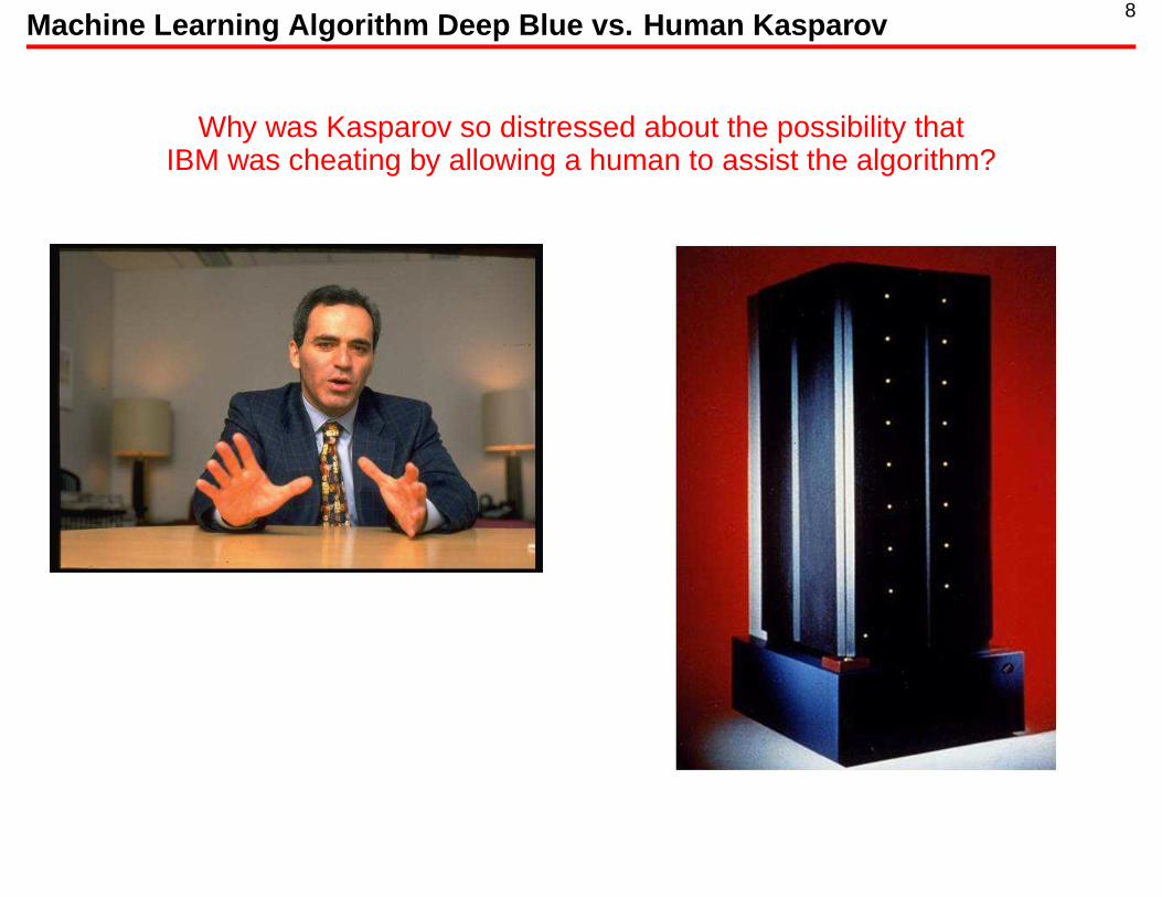
8Machine Learning Algorithm Deep Blue vs. Human Kasparov
Why was Kasparov so distressed about the possibility thatIBM was cheating by allowing a human to assist the algorithm?

9IBM Machine Learning System Deep Blue vs. Human Kasparov
Why was Kasparov so distressed about the possibility thatIBM was cheating by allowing a human to assist the algorithm?
He knew he had no chance to beat a human-machine combination
The immense tactical power of the IBMmachine learning system
The strategic power, much less than hisown, of a grand master

10Conclusion
MATHEMATICAL METHODS
&
VISUALIZATION METHODS
ARE
SYMBIOTIC
11Plan for this Talk
Visualization Databases for Large Complex Datasets
Just a few minutes in this talk
Paper in Journal of Machine Learning Research (AISTATS 2009 Proceedings)
Web site with live examples: ml.stat.purdue.edu/vdb/
Approach to visualization that fosters comprehensive analysis of large complexdatasets

12Plan for this Talk
The ed Method for Nonparametric Density Estimation & Diagnostic Checking
Current work• describe here to make the case for a tight coupling of a mathematical method
and visualization methods
Addresses the 50 year old topic of nonparametric density estimation
50 years of kernel density estimates and very little visualization for diagnosticchecking to see if the density patterns are faithfully represented
A new mathematical method built, in part, to enable visualization
Results• much more faithful following of density patterns in data• visualization methods for diagnostic checking• simple finite sample statistical inference

13Visualization Databases for Large Complex Datasets
Saptarshi Guha Paul Kidwell Ryan Hafen William Cleveland
Department of Statistics, Purdue University

14Visualization Databases for Large Complex Datasets
Comprehensive analysis of large complex database that preserves theinformation in the data is greatly enhanced by a visualization database (VDB)
VDB• many displays• some with many pages• often with many panels per page
A large multi-page display for a singledisplay method• results from parallelizing the data• partition the data into subsets• sample the subsets• apply the visualization method to
each subset in the sample, typicallyone per panel
Time of the analyst• not increased by choosing a large
sample over a small one• display viewers can be designed to
allow rapid scanning: animation withpunctuated stops
• Often, it is not necessary to viewevery page of a display
Display design• to enhance rapid scanning• attention of effortless gestalt
formation that conveys informationrather than focused viewing

15Visualization Databases for Large Complex Datasets
Already successful just with off-the-shelf tools and simple concepts
Can be greatly improved by research in visualization methods that targets VDBs andlarge displays
Our current research projects• subset sampling methods• automation algorithms for choosing basic display elements• display design for gestalt formation

16RHIPE
Our approach to VDBs allows embarrassingly parallel computation
Large amounts of computer time can be saved by distributed computingenvironments
One is RHIPE (ml.stat.purdue.edu/rhipe)• Saptarshi Guha, Purdue Statistics• R-Hadoop Integrated Processing Environment• Greek for “in a moment”• pronounced “hree pay”
A recent merging of the R interactive environment for data analysis(www.R-project.org) and the Hadoop distributed file system and compute engine(hadoop.apache.org)
Public domain
A remarkable achievement that has had a dramatic effect on our ability to computewith large data sets

17The ed Method for Nonparametric Density Estimation & Diagnostic Checking
Ryan Hafen William S. Cleveland
Department of Statistics, Purdue University

18Normalized British Income Data (7201 observations)
f−value
Brit
ish
Inco
me
0
2
4
6
8
0.0 0.2 0.4 0.6 0.8 1.0

19Kernel Density Estimation (KDE): Most-Used Method
Let xj for j = 1 to m be the observations, ordered from smallest to largest
Fixed-bandwidth kernel density estimatewith bandwidth h
Kernel K(u) ≥ 0,∫
∞
−∞K(u)du = 1
f(x) =1
mh
m∑
j=1
K(
x− xj
h
)
K often unit normal probability density,so h = standard deviation
xj closer to x adds more to f(x) than afurther xj
As the bandwidth h increases, f(x)gets smoother

20KDE for Incomes: Gaussian Kernel, Sheather-Jones h
British Income
Den
sity
0.0
0.2
0.4
0.6
0.8
0 1 2 3

21Three Problems of Nonparametric Density Estimation: Problem 1
We want• an estimate to faithfully follow the density patterns in the data• tools that convince us this is happening with our current set of data
There are a few reasonable things• plot estimates with different bandwidths, small to large• model selection criteria• SiZer (Chaudhuri and Marron)
Problem 1: There does not exist a set of comprehensive diagnostic tools.

22Kernel Density Estimates with Gaussian Kernel for Income Data
British Income
Den
sity
0.0
0.2
0.4
0.6
0.8
−1 0 1 2 3 4 5
0.018 0.033
0.061
0.0
0.2
0.4
0.6
0.8
0.1110.0
0.2
0.4
0.6
0.8
0.202
−1 0 1 2 3 4 5
0.368
23Bandwidth Selection Criterion
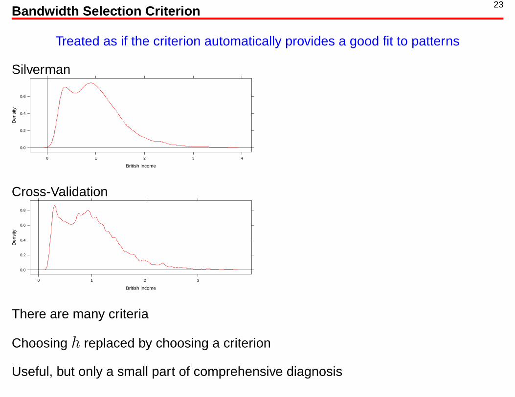
Treated as if the criterion automatically provides a good fit to patterns
Silverman
British Income
Den
sity
0.0
0.2
0.4
0.6
0 1 2 3 4
Cross-Validation
British Income
Den
sity
0.0
0.2
0.4
0.6
0.8
0 1 2 3
There are many criteria
Choosing h replaced by choosing a criterion
Useful, but only a small part of comprehensive diagnosis

24Three Problems of Nonparametric Density Estimation: Problem 2
KDEs are simple and can be made to run very fast, which make us want to use them
Price for the simplicity
Discussed extensively in the literature

25Three Problems of Nonparametric Density Estimation: Problem 2
E(f(x)) =∫
f(x − u)K(u)du, K(u) ≥ 0
This expected value can be far from f(x)• chop peaks• fill in valleys• underestimate density at data boundaries when there is a sharp cutoff in density
(e.g., the world’s simplest density, a uniform)
General assessment: remedies such as changing h or K with x do not fix theproblems, and introduce others
Problem 2: KDEs have much trouble following faithfully the density patterns in data.

26The Three Problems of Nonparametric Density Estimation: Problem 3
Problem 3: Very little technology for statistical inference.

27Regression Analysis (Function Estimation)
Not the impoverished situation of nonparametric density estimation
For example the following model:
yi = g(xi) + εi
• yi for i = 1 to n are measurements of a response
• xi is a p-tuple of measurements of p explanatory variables
• εi are error terms: independent, identically distributed with mean 0
Regression analysis has a wealth of models, mathematical methods,visualization methods for diagnostic checking, and inference technology

28The ed Method for Density Estimation
Take a model building approach
Turn density estimation to a regression analysis to exploit the rich environment foranalysis
In addition seek to make the regression simple by fostering εi that have a normaldistribution
In fact, it is even more powerful than most regression settings because we know theerror variance

29British Income Data: The Modeling Begins Right Away
f−value
Brit
ish
Inco
me
0
2
4
6
8
0.0 0.2 0.4 0.6 0.8 1.0

30Log British Income Data: The Modeling Begins Right Away
f−value
Log
base
2 B
ritis
h In
com
e
−6
−4
−2
0
2
0.0 0.2 0.4 0.6 0.8 1.0

31British Income: The Modeling Begins Right Away
Observations used for nonparametric density estimation• income less than 3.75• log base 2 income larger than −2.75• reduces the number of observations by 39 to 7162
Not realistic to suppose we can get good relative density estimates in these tails bynonparametric methods
Incomes: xj normalized pounds sterling (nps) for j = 1 to m = 7162, ordered fromsmallest to largest

32Histogram of British Incomes
Consider a histogram interval with length g
Estimate of density for the interval is
κ/m
g
fraction of observations
nps
g is fixed and think of κ as a random variable

33Order Statistics and Their Gaps
xj normalized pounds sterling (nps) for j = 1 to m = 7162, ordered from smallestto largest
Order statistic κ-gaps:
g(κ)1 = xκ+1 − x1
g(κ)2 = x2κ+1 − xκ+1
g(κ)3 = x3κ+1 − x2κ+1
...
For κ = 10:
g(10)1 = x11 − x1
g(10)2 = x21 − x11
g(10)3 = x31 − x21
...
Gaps have units nps
Number of observation in each interval is κ

34Balloon Densities
Gaps: g(κ)i = xiκ+1 − x(i−1)κ+1, i = 1, 2, . . . , n
b(κ)i =
κ/m
g(κ)i
fraction of observations
nps
=κ
xiκ+1 − x(i−1)κ+1
fraction of observations
nps
g(κ)i is positioned at the midpoint of the gap interval [x(i−1)κ+1, xiκ+1]
x(κ)i =
xiκ+1 + x(i−1)κ+1
2nps
Now κ is fixed and we think of g(κ)i as a random variable

35A Very Attractive Property of the Log Balloon Estimate
y(κ)i = log(b
(κ)i ), i = 1, . . . , n
Distributional Properties: The “Theory”
“Approximately” independent and distributed like a constant plus the log of achi-squared distribution with 2κ degrees of freedom
E(y(κ)i ) = log f(x
(κ)i ) + log κ− ψ0(κ)
Var(y(κ)i ) = ψ1(κ)
ψ0 = digamma function ψ1 = trigamma function

36ed Step 1: Log Balloon Densities
Start with the log balloon densities as “the raw data”
Two considerations in the choice of κ
(1) small enough that there is as little distortion of the density as possible by theaveraging that occurs
(2) large enough that y(κ)i is approximately normal
• κ = 10 is quite good and κ = 20 nearly perfect (in theory)• we can give this up and even take κ = 1 but next steps are more complicated

37ed: Log Balloon Densities vs. Gap Midpoints for Income with κ = 10
British Income
Log
Den
sity
−5
−4
−3
−2
−1
0
1 2 3

38ed Step 2: Smooth Log Balloon Densities Using Nonparametric Regression
British Income
Den
sity
−4
−2
0
1 2 3

39ed Step 2
Smooth y(κ)i as a function of x
(κ)i using nonparametric regression: loess
Fit polynomials locally of degree δ in a moving fashion like a moving average of atime series
Bandwidth parameter 0 < α ≤ 1
Fit at x uses the [αn] closest points to x, the neighborhood of x
Weighted least-squares fitting where weights decrease to 0 as distances ofneighborhood points increase to the neighborhood boundary
Loess possesses all of the statistical-inference technology of parametric fitting forlinear models

40ed: Three Tuning Parameters
κ: gap length
α: bandwidth
δ: degree of polynomial in local fitting

41Notational Change
Midpoints of gap intervals: x(κ)i → xi
Log balloon densities: y(κ)i → yi
42ed Step 2
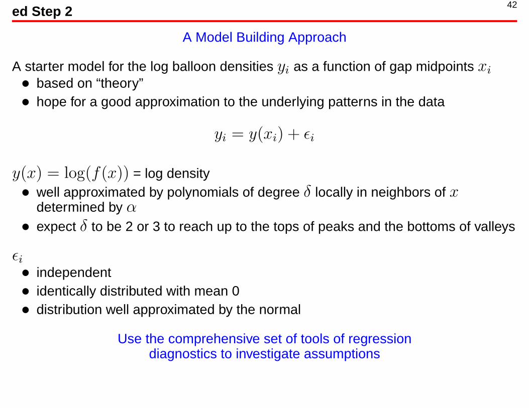
A Model Building Approach
A starter model for the log balloon densities yi as a function of gap midpoints xi
• based on “theory”• hope for a good approximation to the underlying patterns in the data
yi = y(xi) + εi
y(x) = log(f(x)) = log density• well approximated by polynomials of degree δ locally in neighbors of x
determined by α• expect δ to be 2 or 3 to reach up to the tops of peaks and the bottoms of valleys
εi• independent• identically distributed with mean 0• distribution well approximated by the normal
Use the comprehensive set of tools of regressiondiagnostics to investigate assumptions

43Model Diagnostics
Important quantities used in carrying out diagnostics
y(x) = ed log density fit from nonparametric regression
yi = y(xi) = fitted values at xi = gap midpoints
εi = yi − yi = residuals
f(x) = exp(y(x)) = ed density estimate
Loess possesses all of the statistical-inferencetechnology of parametric linear regression
σ2ε = estimate of error variance
• in theory, variance = γ1(κ), which is 0.105 for κ = 10
ν = equivalent degrees of freedom of the fit (number of parameters)

44ed Log Raw Density Estimate for Income: Fit vs. Income
British Income
Den
sity
−6
−4
−2
0
1 2 3
0.022
0.12
1 2 3
0.172
0.252
1 2 3
0.322
−6
−4
−2
0
0.42

45ed Log Density Estimate for Income: Residuals vs. Income
British Income
Den
sity
−0.5
0.0
0.5
1.0
1 2 3
0.022
0.12
1 2 3
0.172
0.252
1 2 3
0.322
−0.5
0.0
0.5
1.0
0.42

46ed Density Estimate for Income: Fit vs. Income
British Income
Den
sity
0.0
0.2
0.4
0.6
0.8
1.0
0 1 2 3 4
0.022
0.12
0.172
0.0
0.2
0.4
0.6
0.8
1.0
0.252
0.0
0.2
0.4
0.6
0.8
1.0
0.322
0 1 2 3 4
0.42

47ed Log Density Estimate for Income: Residual Variance vs. Degrees Freedom
ν
Res
idua
l Var
ianc
e E
stim
ate
0.100
0.105
0.110
10 15 20 25 30 35
degree 1 degree 2 degree 3

48Mallows Cp Model Selection Criterion
A visualization tool for showing the trade-off of bias and variance, which is far moreuseful than just a criterion that one minimizes or is optimizing
M : an estimate of mean-squared error
ν: degrees of freedom of fit
M estimates
Bias Sum of Squares
σ2+
Variance Sum of Squares
σ2
M =
∑
i ε2i
σ2(ε)− (n− ν) + ν
E(M) ≈ ν when the fit follows the pattern in the data
The amount by which M exceeds ν is an estimate of the bias
Cp: M vs. ν

49ed Log Density Estimate for Income: Cp Plot
ν
M
20
40
60
80
10 15 20 25 30 35
degree 1 degree 2 degree 3

50Model Selection for British Incomes
From Cp plot, plots of residuals, and plots of fits
Gap size: κ = 10
Polynomial degree: δ = 2
Bandwidth parameter: α = 0.16
Equivalent degrees of freedom: ν = 19

51ed Log Density Estimate for Income: Fit vs. Income
British Income
Den
sity
−4
−2
0
1 2 3

52ed Log Density Estimate for Income: Residuals vs. Income
British Income
Den
sity
−0.5
0.0
0.5
1.0
1 2 3
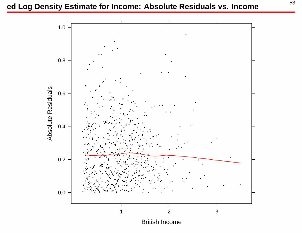
53ed Log Density Estimate for Income: Absolute Residuals vs. Income
British Income
Abs
olut
e R
esid
uals
0.0
0.2
0.4
0.6
0.8
1.0
1 2 3

54ed Log Density Estimate for Income: Lag 1 Residual Correlation Plot
Residual (i)
Res
idua
l (i−
1)
−0.5
0.0
0.5
1.0
−0.5 0.0 0.5 1.0

55ed Log Density Estimate for Income: Normal Quantile Plot of Residuals
Normal Quantiles
Res
idua
ls
−1.0
−0.5
0.0
0.5
1.0
−0.5 0.0 0.5 1.0

56ed Density Estimate and KDE for Income: Fits vs. Income
British Income
Den
sity
0.0
0.2
0.4
0.6
0.8
0 1 2 3
Sheather−Jones
0.0
0.2
0.4
0.6
0.8
Ed

57ed Log Density Estimate and Log KDE for Income: Residuals vs. Income
British Income
Res
idua
ls
−0.5
0.0
0.5
1.0
1 2 3
Ed
1 2 3
Sheather−Jones

58ed Log Density Estimate for Income: 99% Pointwise Confidence Intervals
Log
Den
sity
−1.5
−1.0
−0.5
0.0
0.5 1.0 1.5
British Income
−0.100.000.10
0.5 1.0 1.5

59Queuing Delays of Internet Voice-over-IP Traffic
264583 observations
From a study of quality of service for different traffic loads
Semi-empirical model for generating traffic
Simulated queueing on a router

60Silverman Bandwidth KDE for Delay: Fit vs. Delay
Delay (ms)
Den
sity
0
1
2
3
4
5
6
0.0 0.1 0.2 0.3 0.4 0.5 0.6

61Silverman Bandwidth Log KDE for Delay: Residuals vs. Delay
Delay (ms)
Res
idua
l
−1.5
−1.0
−0.5
0.0
0.5
1.0
0.0 0.1 0.2 0.3 0.4

62ed Log Raw Density Estimates for Delay: κ = 100 Because of Ties
Delay (ms)
Log
Den
sity
−4
−2
0
2
0.0 0.1 0.2 0.3 0.4

63ed Log Density Estimates for Delay: 3 Independent Fits for Three Intervals
Polynomial degrees δ and bandwidths α for loess fits
Interval 1: δ = 1, α = 0.75
Interval 2: δ = 2, α = 0.5
Interval 3: δ = 1, α = 1.5

64ed Log Density Estimates for Delay: 3 Fits vs. Delay
Delay (ms)
Den
sity
−4
−2
0
2
0.0 0.1 0.2 0.3 0.4

65ed Log Density Estimates, 3 Fits for Delay: Residuals vs. Delay
Delay (ms)
Den
sity
−0.5
0.0
0.5
1.0
0.0 0.1 0.2 0.3 0.4
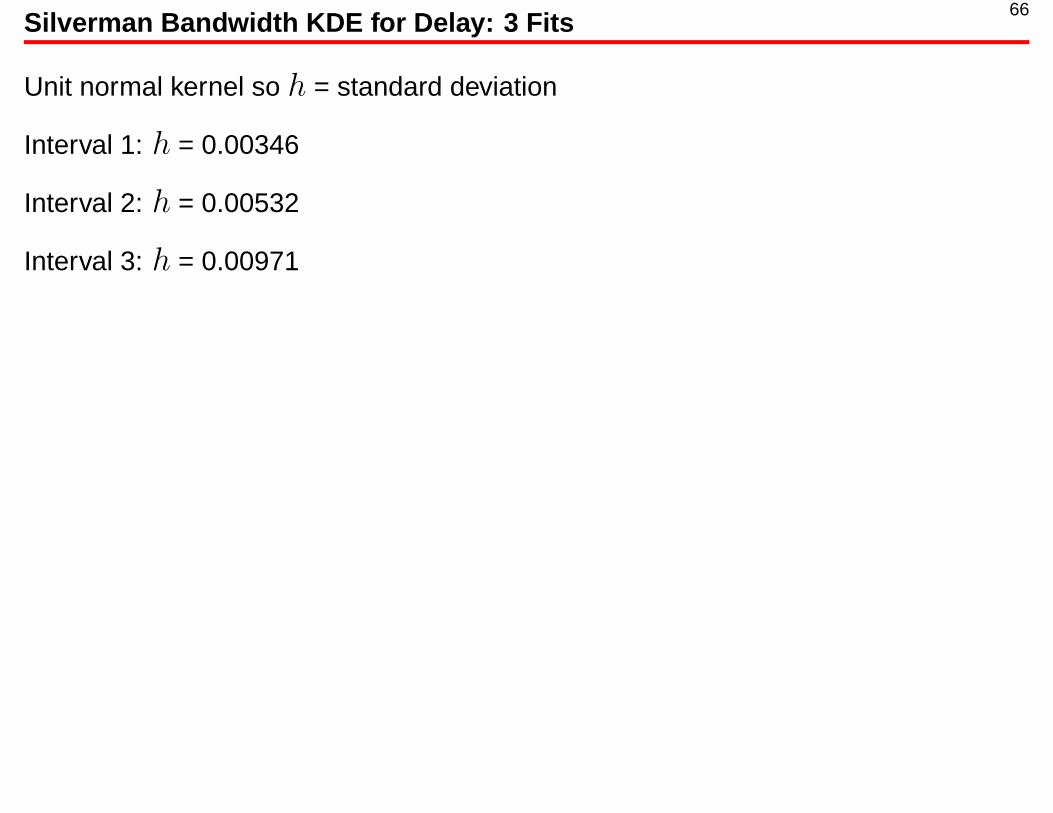
66Silverman Bandwidth KDE for Delay: 3 Fits
Unit normal kernel so h = standard deviation
Interval 1: h = 0.00346
Interval 2: h = 0.00532
Interval 3: h = 0.00971

67Silverman Bandwidth KDE for Delay: 3 Fits vs. Delay
Delay (ms)
Log
Den
sity
−4
−2
0
2
0.0 0.1 0.2 0.3 0.4
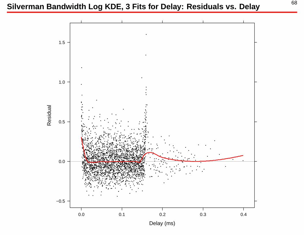
68Silverman Bandwidth Log KDE, 3 Fits for Delay: Residuals vs. Delay
Delay (ms)
Res
idua
l
−0.5
0.0
0.5
1.0
1.5
0.0 0.1 0.2 0.3 0.4

69Computation
We use existing algorithms for loess to get faster computations for ed than directcomputation
Still, are the ed computations fast enough, especially for extensions to higherdimensions?
Alex Gray and collaborators have done some exceptional work in algorithms for fastcomputation of KDEs and nonparametric regression
Nonparametric Density Estimation: Toward Computational Tractability. Gray, A. G.and Moore, A. W. In SIAM International Conference on Data Mining, 2003. Winnerof Best Algorithm Paper Prize.
How can we tailor this to our needs here?

70RHIPE
ed presents embarrassingly parallel computation
Large amounts of computer time can be saved by distributed computingenvironments
One is RHIPE (ml.stat.purdue.edu/rhipe)• Saptarshi Guha, Purdue Statistics• R-Hadoop Integrated Processing Environment• Greek for “in a moment”• pronounced “hree pay”
A recent merging of the R interactive environment for data analysis(www.R-project.org) and the Hadoop distributed file system and compute engine(hadoop.apache.org)
Public domain
A remarkable achievement that has had a dramatic effect on our ability to computewith large data sets