Williamson, S. J., Griffo, A., Stark, B. H., & Booker, J. D. (2016). Acontroller for single-phase parallel inverters in a variable-head pico-hydropower off-grid network. Sustainable Energy, Grids and Networks, 5,114-124. DOI: 10.1016/j.segan.2015.11.006

Peer reviewed version

Link to published version (if available):10.1016/j.segan.2015.11.006

Link to publication record in Explore Bristol ResearchPDF-document

University of Bristol - Explore Bristol ResearchGeneral rights

This document is made available in accordance with publisher policies. Please cite only the publishedversion using the reference above. Full terms of use are available:http://www.bristol.ac.uk/pure/about/ebr-terms

1

A Controller for Single-Phase Parallel Inverters in a Variable-Head Pico-Hydropower Off-Grid

Network

S. J. Williamson a*, A. Griffo b, B. H. Stark a, J. D. Booker a

a Faculty of Engineering, University of Bristol, Bristol, BS8 1TR, UK

b Department of Electrical & Electronic Engineering, University of Sheffield, Sheffield, S1 3JD, UK

* Corresponding Author: Tel: +44 117 331 5464, Email: sam.williamson@bristol.ac.uk

Abstract

The majority of off-grid pico-hydropower systems use a single turbine and generator, connected directly

to an AC network resulting in clusters of isolated, power-limited, single failure-prone networks. The use of

inverters has been previously proposed in order to decouple the turbine’s rotational speed from the network

frequency in these remote microgrids. This facilitates the use of multiple generators and the creation of

expandable, reliable networks with redundancy. This paper presents an inverter controller for this situation,

and addresses a combination of challenges that is specific to expandable pico-hydropower networks in

geographically dispersed remote communities. Multiple variable-head turbines are connected to a network,

whose individual local hydraulic heads vary due to flow changes over the seasons, and the network has no

single generator that dominates and no master controller, but instead identical independent controllers that

do not communicate. The controller presented here uses an output voltage and frequency droop controller,

with inner synchronous reference frame control loops for the fundamental voltage and current. The control

coefficients are automatically adjusted to the available local hydraulic head. Simulation and experimental

results show that the power is shared amongst generators, proportionally to the locally available power, in

steady and dynamic situations. Harmonic compensation loops are proposed: these reduce the output total

harmonic distortion (THD) of a single inverter from 9.53% to 1.45% for a non-linear load. Geographically

distributed operation in resistive networks is investigated, and the results show that the controller achieves

plug-and-play capability for remote off-grid networks with multiple and different pico-hydropower

generators.

Keywords – Parallel inverter control, Pico hydropower, Single-phase, Droop control, Rural electrification.

2

1. INTRODUCTION

Pico hydropower has been used for many decades as a method of delivering rural electrification. It has

been shown to be a cost effective method of off-grid electricity generation, especially in hilly and

mountainous regions [1]. A standard pico-hydro system is a stand-alone unit, comprising a turbine driving a

generator, a shunt controller, known as an electronic load controller (ELC) regulating either the voltage or

frequency output, and a low-voltage distribution system with consumer loads, such as lighting, mobile

phone chargers and radios [2, 3]. The turbine is designed to operate at a constant speed to generate the grid

frequency; the ELC maintaining a constant load on generator. Fluctuations in the environmental conditions,

such as a drop in flow rate or head, can cause the system to shut down. Over time, consumer demand on the

system increases as they purchase more electrical equipment, up to the point where the increased demand

causes severe voltage drop in peak load times and often the circuit breaker at the generator to trip.

Therefore, there is a demand for methods to connect multiple hydropower generators and expand the off-

grid network as more capital becomes available. A straightforward method is to connect micro-hydro units

through synchronizer units directly to the grid. This is implemented in a recent 11 kV off-grid network

containing six micro-hydro units, constructed in Western Nepal by the Alternative Energy Promotion

Centre [4]. Due to the direct connection of induction generators, power quality and sharing are not

controlled, and changes in head strongly affect power sharing, risking a loss of synchronization. A potential

solution is to use a power electronic interface per turbine. For example, a rectifier is followed by a DC-DC

converter that feeds the DC link of a single-phase inverter. This allows the turbine to operate at its optimal

head- and flow-dependent frequency, with grid voltage and power flow regulation performed using

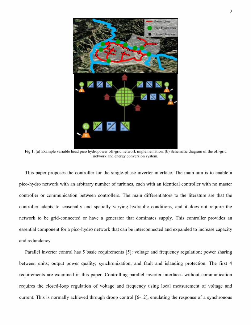
techniques similar to those reported for grid-connected and off-grid microgrids. An example system

implementation in a rural off-grid network is shown in Fig. 1 (a), with the schematic system diagram shown

in Fig. 1 (b).

3

Fig 1. (a) Example variable head pico hydropower off-grid network implementation. (b) Schematic diagram of the off-grid

network and energy conversion system.

This paper proposes the controller for the single-phase inverter interface. The main aim is to enable a

pico-hydro network with an arbitrary number of turbines, each with an identical controller with no master

controller or communication between controllers. The main differentiators to the literature are that the

controller adapts to seasonally and spatially varying hydraulic conditions, and it does not require the

network to be grid-connected or have a generator that dominates supply. This controller provides an

essential component for a pico-hydro network that can be interconnected and expanded to increase capacity

and redundancy.

Parallel inverter control has 5 basic requirements [5]: voltage and frequency regulation; power sharing

between units; output power quality; synchronization; and fault and islanding protection. The first 4

requirements are examined in this paper. Controlling parallel inverter interfaces without communication

requires the closed-loop regulation of voltage and frequency using local measurement of voltage and

current. This is normally achieved through droop control [6-12], emulating the response of a synchronous

4

generator connected to a grid. There are alternative methods proposed in the literature, such as augmenting

the control with an average power control technique [13] or controlling the inverter to behave as a

synchronous machine [14, 15]. A secondary control loop can also be used to restore the network voltage or

frequency to its nominal levels [16].

Utilizing droop control requires a trade-off between the voltage and frequency regulation and the power

sharing capability of the system [7]. In the approach reported on here, loose regulation is required to

achieve power sharing between geographically-dispersed generators on a low-voltage (resistive) network.

Power sharing between units with different input power can be improved by adjusting the droop

coefficients [8] and virtual impedance [9] with the input power. The output power quality can be controlled

using a single virtual impedance [16] or set of band-pass filters in the virtual output impedance [7] or

through a series of harmonic droop controllers [17]. Synchronization between parallel inverters has been

achieved through using a large variable physical [10] or virtual [7] impedance or a phase-locked-loop [18].

There are many examples in the literature of parallel inverter control schemes, such as those in the

references above, but none that have been interfaced with a variable-input-power pico-hydro system.

The paper is structured as follows: Section 2 develops the control system, derives the inner current,

voltage and harmonic controller transfer functions, and shows respective bode plots. The section also

addresses: automated adjustment of droop coefficients and virtual output impedance as a function of the

available turbine power; power sharing proportional to each unit’s available power; plug-and-play

capabilities enabling interconnection of additional units, each capable of working in load sharing or grid

forming mode; and compensation of harmonic distortion caused by nonlinear loads. Section 3 demonstrates

the controller performance by simulation. Section 4 describes the experimental test facility, and finally

Section 5 presents scale experimental results for voltage quality and power sharing ratios with unequal

transmission line length and source power.

5

2. CONTROL SYSTEM DESIGN

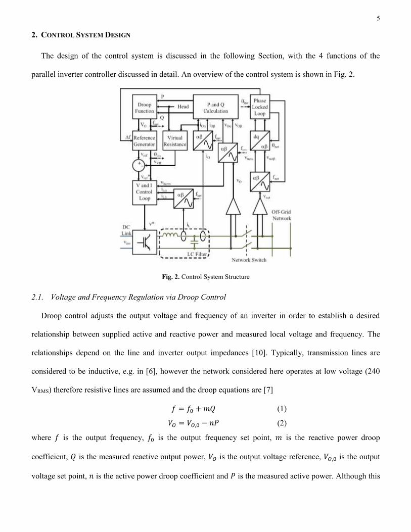
The design of the control system is discussed in the following Section, with the 4 functions of the

parallel inverter controller discussed in detail. An overview of the control system is shown in Fig. 2.

Fig. 2. Control System Structure

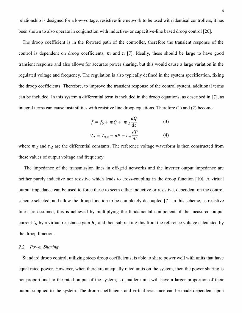
2.1. Voltage and Frequency Regulation via Droop Control

Droop control adjusts the output voltage and frequency of an inverter in order to establish a desired

relationship between supplied active and reactive power and measured local voltage and frequency. The

relationships depend on the line and inverter output impedances [10]. Typically, transmission lines are

considered to be inductive, e.g. in [6], however the network considered here operates at low voltage (240

VRMS) therefore resistive lines are assumed and the droop equations are [7]

𝑓 = 𝑓0 + 𝑚𝑄 (1)

𝑉𝑂 = 𝑉𝑂,0 − 𝑛𝑃 (2)

where 𝑓 is the output frequency, 𝑓0 is the output frequency set point, 𝑚 is the reactive power droop

coefficient, 𝑄 is the measured reactive output power, 𝑉𝑂 is the output voltage reference, 𝑉𝑂,0 is the output

voltage set point, 𝑛 is the active power droop coefficient and 𝑃 is the measured active power. Although this

6

relationship is designed for a low-voltage, resistive-line network to be used with identical controllers, it has

been shown to also operate in conjunction with inductive- or capacitive-line based droop control [20].

The droop coefficient is in the forward path of the controller, therefore the transient response of the

control is dependent on droop coefficients, 𝑚 and 𝑛 [7]. Ideally, these should be large to have good

transient response and also allows for accurate power sharing, but this would cause a large variation in the

regulated voltage and frequency. The regulation is also typically defined in the system specification, fixing

the droop coefficients. Therefore, to improve the transient response of the control system, additional terms

can be included. In this system a differential term is included in the droop equations, as described in [7], as

integral terms can cause instabilities with resistive line droop equations. Therefore (1) and (2) become

𝑓 = 𝑓0 + 𝑚𝑄 + 𝑚𝑑

𝑑𝑄

𝑑𝑡 (3)

𝑉𝑂 = 𝑉𝑂,0 − 𝑛𝑃 − 𝑛𝑑

𝑑𝑃

𝑑𝑡 (4)

where 𝑚𝑑 and 𝑛𝑑 are the differential constants. The reference voltage waveform is then constructed from

these values of output voltage and frequency.

The impedance of the transmission lines in off-grid networks and the inverter output impedance are

neither purely inductive nor resistive which leads to cross-coupling in the droop function [10]. A virtual

output impedance can be used to force these to seem either inductive or resistive, dependent on the control

scheme selected, and allow the droop function to be completely decoupled [7]. In this scheme, as resistive

lines are assumed, this is achieved by multiplying the fundamental component of the measured output

current 𝑖𝑂 by a virtual resistance gain 𝑅𝑉 and then subtracting this from the reference voltage calculated by

the droop function.

2.2. Power Sharing

Standard droop control, utilizing steep droop coefficients, is able to share power well with units that have

equal rated power. However, when there are unequally rated units on the system, then the power sharing is

not proportional to the rated output of the system, so smaller units will have a larger proportion of their

output supplied to the system. The droop coefficients and virtual resistance can be made dependent upon

7

the input power, which assists in achieving accurate power sharing proportional to the unit’s available input

power [8, 9], which have been used for UPS inverters. In the presented case, the input power is dependent

on the head at the turbine. Therefore, a model for the turbine can be used to determine the maximum power

available at the turbine for a given head, P(TURB,MAX) (H)., such as those found in [20-23]. Alternatively, if

there is experimental data for the turbine performance across its head range, a look-up table of the

maximum available turbine power can be included for each measured head. For this paper, a low-head

Turgo turbine model theoretically derived and experimentally validated in [20] is used, and therefore the

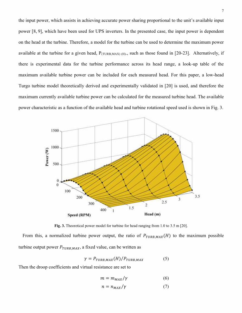
maximum currently available turbine power can be calculated for the measured turbine head. The available

power characteristic as a function of the available head and turbine rotational speed used is shown in Fig. 3.

Fig. 3. Theoretical power model for turbine for head ranging from 1.0 to 3.5 m [20].

From this, a normalized turbine power output, the ratio of 𝑃𝑇𝑈𝑅𝐵,𝑀𝐴𝑋(𝐻) to the maximum possible

turbine output power 𝑃𝑇𝑈𝑅𝐵,𝑀𝐴𝑋, a fixed value, can be written as

𝛾 = 𝑃𝑇𝑈𝑅𝐵,𝑀𝐴𝑋(𝐻) 𝑃𝑇𝑈𝑅𝐵,𝑀𝐴𝑋⁄ (5)

Then the droop coefficients and virtual resistance are set to

𝑚 = 𝑚𝑀𝐴𝑋 𝛾⁄ (6)

𝑛 = 𝑛𝑀𝐴𝑋 𝛾⁄ (7)

8

𝑅𝑉 = 𝑅𝑉,𝑀𝐴𝑋 𝛾⁄ (8)

where 𝑚𝑀𝐴𝑋 and 𝑛𝑀𝐴𝑋 are defined from the regulated range of frequency and output voltage and the

maximum output active and reactive powers and 𝑅𝑉,𝑀𝐴𝑋 is the maximum power virtual resistance. In this

way, as reduces the gradients of the droop curves become steeper. So in the case of the 𝑃 vs. 𝑉𝑂 droop

curve, for the same output voltage, the active power delivered is reduced.

The stability of the system resulting from the interconnection of multiple generation units with

dynamically changing heads is potentially challenging, with short term system stability and longer term

power system stability. In this paper, we assume that the flow rate is nearly constant, with changes

happening over a significantly longer time-scale than the proposed controller, e.g. days vs. tens of

milliseconds. Under this reasonable assumption the instantaneous output power control and the load

management can be assumed to be decoupled. Load management issues can then potentially be guaranteed

with an appropriate supply/demand management strategy.

2.3. Power Measurement

The droop function, (3) and (4), needs the line-cycle-averaged active and reactive powers to calculate

the output voltage and frequency. In 3-phase systems this can be achieved by using the Clarke transform to

convert the line values into orthogonal and components. The instantaneous powers are calculated using

𝑃 = (𝑣𝑂𝛼𝑖𝑂𝛼 + 𝑣𝑂𝛽𝑖𝑂𝛽) 2⁄ (9)

𝑄 = (𝑣𝑂𝛽𝑖𝑂𝛼 − 𝑣𝑂𝛼𝑖𝑂𝛽) 2⁄ (10)

which are used as inputs for the droop function. For single-phase systems, there are several different

methods to achieve the conversion between a single-phase sinusoidal signal and components, such as

shifting the signal by 90° using a transport delay [7], integrating the incoming signal [24] or using a

resonant filter [25], which is based on a Second Order Generalised Integrator (SOGI) [18]. A modified

version of this SOGI-based filter is proposed in [26], where an additional gain is included in the orthogonal

() path, and the gains are calculated using a Kalman function. An alternative method using a Reduced

Order Generalised Integrator (ROGI) based filter has been proposed in [27], where the filter is

implemented in the synchronous reference frame which reduces the number of states in the implementation,

9

allowing for a reduced computational overhead. However this can only be implemented for 3-phase

systems as it requires the stationary reference frame components as an input. The method used in this paper

has an identical structure to that presented in [26], but with constant gain values calculated using the

method in [26]. The resonant frequency used in the filter is calculated from the droop function, (3), and is

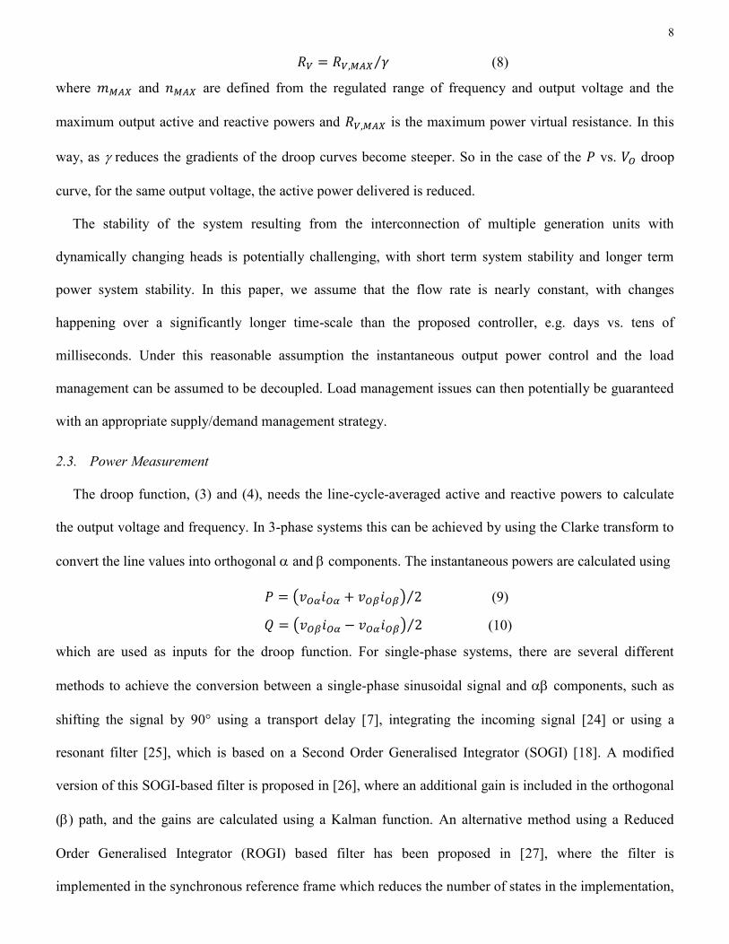
fed into the filter, allowing the filter to adapt to any variation in the grid frequency. The structure of the

SOGI-based filter is shown in Fig. 4 (a).

(a)

(b)

Fig. 4. (a) Second Order Generalised Integrator (SOGI) based filter with additional harmonic loops. (b) Symbolic representation

of SOGI-based filter.

Additional resonant loops can be added to filter any harmonics in the input [28], as shown in Fig. 4 (a)

where a 3rd harmonic loop is included. The harmonics from each additional loop can be extracted and used

if needed. Fig. 4 (b) shows the symbol used for the SOGI-based filter in the following Sections.

2.4. Fundamental Voltage Controller

A second order 𝐿𝐶 filter is assumed at the output of the inverter. Similar to the control structure

commonly employed in three-phase grid connected inverters and active rectifiers [29, 30], a synchronous

reference frame controller is employed here for both the outer output capacitor voltage and inner inductor

current control loops. A similar approach has been used in [11] where the outer voltage loop is transformed

into the synchronous frame, before being returned into the stationary frame for the current control loop.

10

This current loop is a proportional loop with a feed-forward term, which reduces the need for a large gain

to reduce the steady-state error. Similar control strategies are proposed in [31-33], where the systems

described are either already in three-phase or use delays to create the orthogonal component.

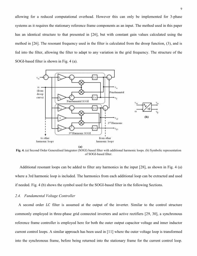
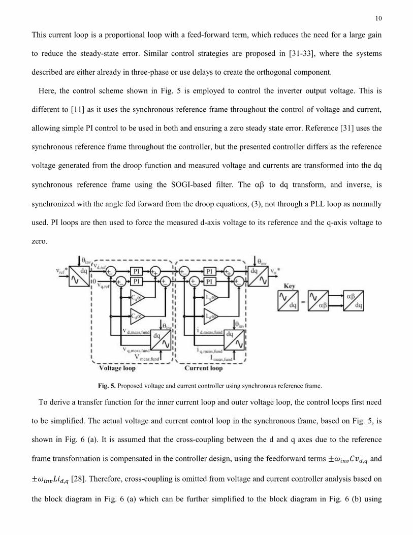
Here, the control scheme shown in Fig. 5 is employed to control the inverter output voltage. This is

different to [11] as it uses the synchronous reference frame throughout the control of voltage and current,

allowing simple PI control to be used in both and ensuring a zero steady state error. Reference [31] uses the

synchronous reference frame throughout the controller, but the presented controller differs as the reference

voltage generated from the droop function and measured voltage and currents are transformed into the dq

synchronous reference frame using the SOGI-based filter. The to dq transform, and inverse, is

synchronized with the angle fed forward from the droop equations, (3), not through a PLL loop as normally

used. PI loops are then used to force the measured d-axis voltage to its reference and the q-axis voltage to

zero.

Fig. 5. Proposed voltage and current controller using synchronous reference frame.

To derive a transfer function for the inner current loop and outer voltage loop, the control loops first need

to be simplified. The actual voltage and current control loop in the synchronous frame, based on Fig. 5, is

shown in Fig. 6 (a). It is assumed that the cross-coupling between the d and q axes due to the reference

frame transformation is compensated in the controller design, using the feedforward terms ±𝜔𝑖𝑛𝑣𝐶𝑣𝑑,𝑞 and

±𝜔𝑖𝑛𝑣𝐿𝑖𝑑,𝑞[28]. Therefore, cross-coupling is omitted from voltage and current controller analysis based on

the block diagram in Fig. 6 (a) which can be further simplified to the block diagram in Fig. 6 (b) using

11

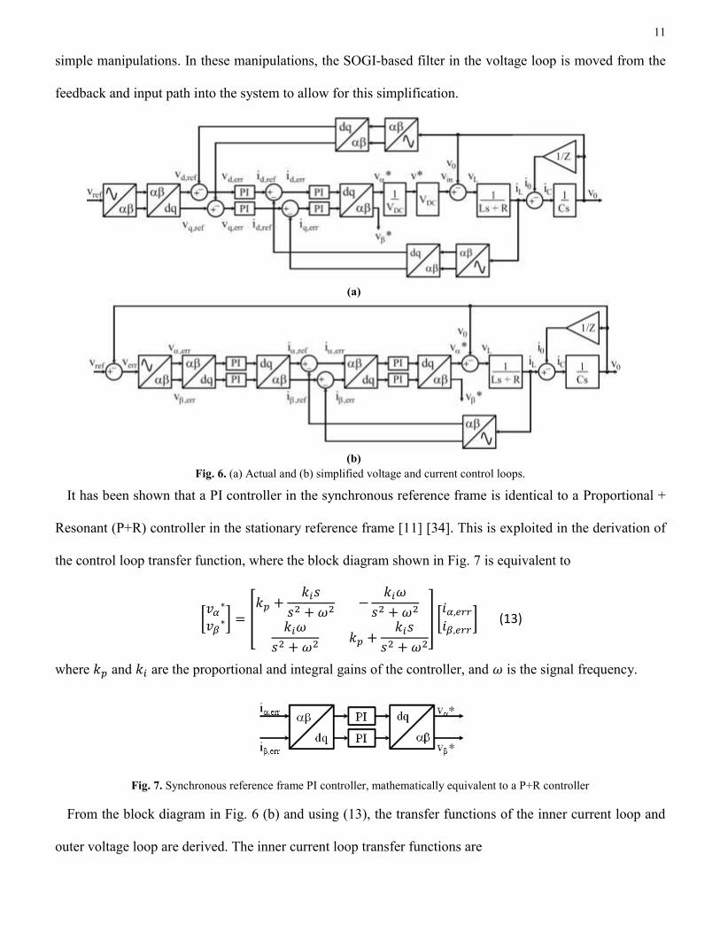
simple manipulations. In these manipulations, the SOGI-based filter in the voltage loop is moved from the

feedback and input path into the system to allow for this simplification.

(a)

(b)

Fig. 6. (a) Actual and (b) simplified voltage and current control loops.

It has been shown that a PI controller in the synchronous reference frame is identical to a Proportional +

Resonant (P+R) controller in the stationary reference frame [11] [34]. This is exploited in the derivation of

the control loop transfer function, where the block diagram shown in Fig. 7 is equivalent to

[𝑣𝛼

∗

𝑣𝛽∗] = [

𝑘𝑝 +𝑘𝑖𝑠

𝑠2 + 𝜔2−

𝑘𝑖𝜔

𝑠2 + 𝜔2

𝑘𝑖𝜔

𝑠2 + 𝜔2𝑘𝑝 +

𝑘𝑖𝑠

𝑠2 + 𝜔2

] [𝑖𝛼,𝑒𝑟𝑟

𝑖𝛽,𝑒𝑟𝑟] (13)

where 𝑘𝑝 and 𝑘𝑖 are the proportional and integral gains of the controller, and 𝜔 is the signal frequency.

Fig. 7. Synchronous reference frame PI controller, mathematically equivalent to a P+R controller

From the block diagram in Fig. 6 (b) and using (13), the transfer functions of the inner current loop and

outer voltage loop are derived. The inner current loop transfer functions are

12

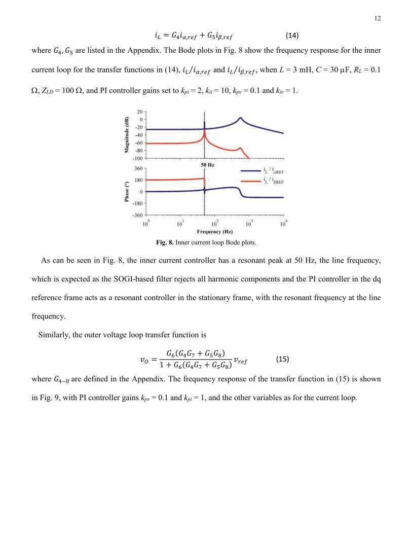
𝑖𝐿 = 𝐺4𝑖𝛼,𝑟𝑒𝑓 + 𝐺5𝑖𝛽,𝑟𝑒𝑓 (14)

where 𝐺4, 𝐺5 are listed in the Appendix. The Bode plots in Fig. 8 show the frequency response for the inner

current loop for the transfer functions in (14), 𝑖𝐿 𝑖𝛼,𝑟𝑒𝑓⁄ and 𝑖𝐿 𝑖𝛽,𝑟𝑒𝑓⁄ , when L = 3 mH, C = 30 F, RL = 0.1

, ZLD = 100 , and PI controller gains set to kpi = 2, kii = 10, kpv = 0.1 and kiv = 1.

Fig. 8. Inner current loop Bode plots.

As can be seen in Fig. 8, the inner current controller has a resonant peak at 50 Hz, the line frequency,

which is expected as the SOGI-based filter rejects all harmonic components and the PI controller in the dq

reference frame acts as a resonant controller in the stationary frame, with the resonant frequency at the line

frequency.

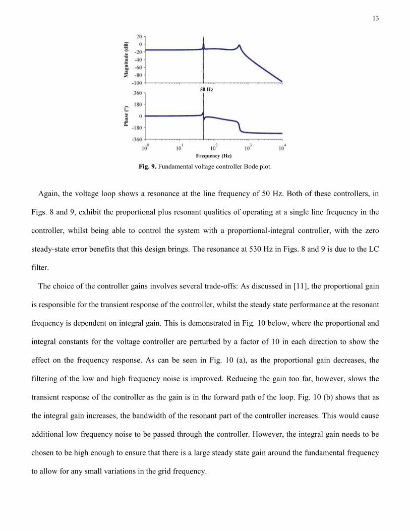
Similarly, the outer voltage loop transfer function is

𝑣𝑂 =𝐺6(𝐺4𝐺7 + 𝐺5𝐺8)

1 + 𝐺6(𝐺4𝐺7 + 𝐺5𝐺8)𝑣𝑟𝑒𝑓 (15)

where 𝐺4−8 are defined in the Appendix. The frequency response of the transfer function in (15) is shown

in Fig. 9, with PI controller gains kpv = 0.1 and kpi = 1, and the other variables as for the current loop.

13

Fig. 9. Fundamental voltage controller Bode plot.

Again, the voltage loop shows a resonance at the line frequency of 50 Hz. Both of these controllers, in

Figs. 8 and 9, exhibit the proportional plus resonant qualities of operating at a single line frequency in the

controller, whilst being able to control the system with a proportional-integral controller, with the zero

steady-state error benefits that this design brings. The resonance at 530 Hz in Figs. 8 and 9 is due to the LC

filter.

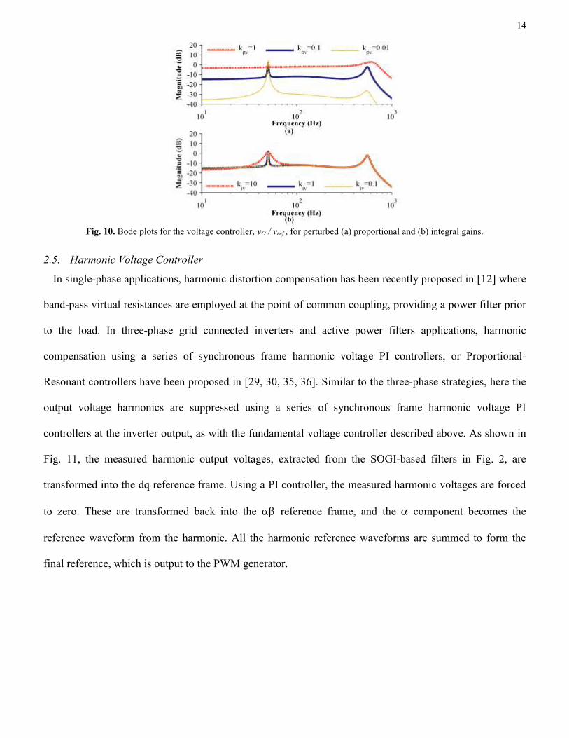
The choice of the controller gains involves several trade-offs: As discussed in [11], the proportional gain

is responsible for the transient response of the controller, whilst the steady state performance at the resonant

frequency is dependent on integral gain. This is demonstrated in Fig. 10 below, where the proportional and

integral constants for the voltage controller are perturbed by a factor of 10 in each direction to show the

effect on the frequency response. As can be seen in Fig. 10 (a), as the proportional gain decreases, the

filtering of the low and high frequency noise is improved. Reducing the gain too far, however, slows the

transient response of the controller as the gain is in the forward path of the loop. Fig. 10 (b) shows that as

the integral gain increases, the bandwidth of the resonant part of the controller increases. This would cause

additional low frequency noise to be passed through the controller. However, the integral gain needs to be

chosen to be high enough to ensure that there is a large steady state gain around the fundamental frequency

to allow for any small variations in the grid frequency.

14

Fig. 10. Bode plots for the voltage controller, vO / vref , for perturbed (a) proportional and (b) integral gains.

2.5. Harmonic Voltage Controller

In single-phase applications, harmonic distortion compensation has been recently proposed in [12] where

band-pass virtual resistances are employed at the point of common coupling, providing a power filter prior

to the load. In three-phase grid connected inverters and active power filters applications, harmonic

compensation using a series of synchronous frame harmonic voltage PI controllers, or Proportional-

Resonant controllers have been proposed in [29, 30, 35, 36]. Similar to the three-phase strategies, here the

output voltage harmonics are suppressed using a series of synchronous frame harmonic voltage PI

controllers at the inverter output, as with the fundamental voltage controller described above. As shown in

Fig. 11, the measured harmonic output voltages, extracted from the SOGI-based filters in Fig. 2, are

transformed into the dq reference frame. Using a PI controller, the measured harmonic voltages are forced

to zero. These are transformed back into the reference frame, and the component becomes the

reference waveform from the harmonic. All the harmonic reference waveforms are summed to form the

final reference, which is output to the PWM generator.

15

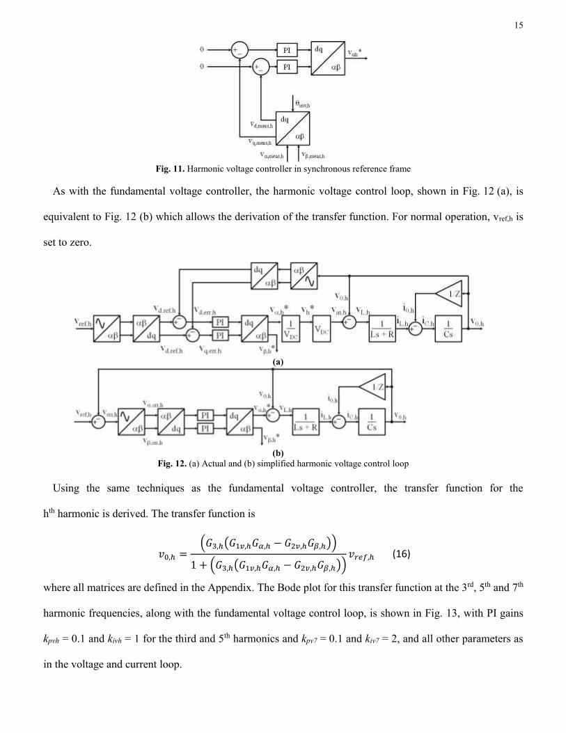
Fig. 11. Harmonic voltage controller in synchronous reference frame

As with the fundamental voltage controller, the harmonic voltage control loop, shown in Fig. 12 (a), is

equivalent to Fig. 12 (b) which allows the derivation of the transfer function. For normal operation, vref,h is

set to zero.

(a)

(b)

Fig. 12. (a) Actual and (b) simplified harmonic voltage control loop

Using the same techniques as the fundamental voltage controller, the transfer function for the

hth harmonic is derived. The transfer function is

𝑣0,ℎ =(𝐺3,ℎ(𝐺1𝑣,ℎ𝐺𝛼,ℎ − 𝐺2𝑣,ℎ𝐺𝛽,ℎ))

1 + (𝐺3,ℎ(𝐺1𝑣,ℎ𝐺𝛼,ℎ − 𝐺2𝑣,ℎ𝐺𝛽,ℎ))𝑣𝑟𝑒𝑓,ℎ (16)

where all matrices are defined in the Appendix. The Bode plot for this transfer function at the 3rd, 5th and 7th

harmonic frequencies, along with the fundamental voltage control loop, is shown in Fig. 13, with PI gains

kpvh = 0.1 and kivh = 1 for the third and 5th harmonics and kpv7 = 0.1 and kiv7 = 2, and all other parameters as

in the voltage and current loop.

16

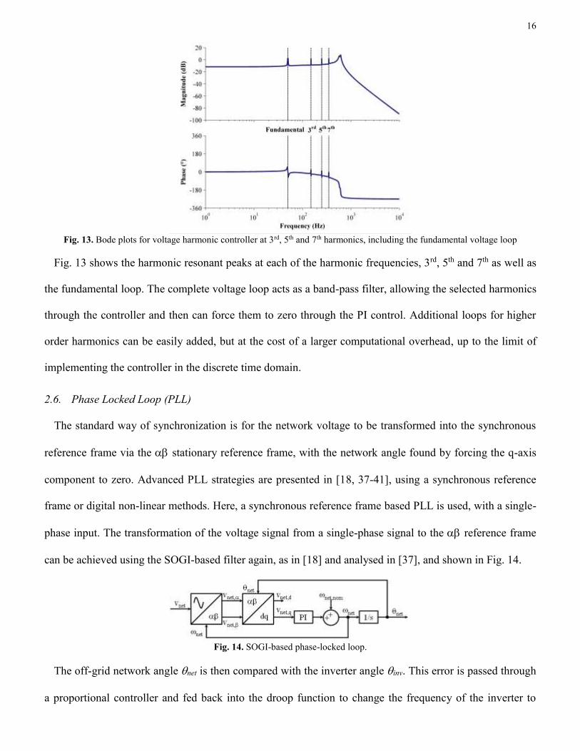
Fig. 13. Bode plots for voltage harmonic controller at 3rd, 5th and 7th harmonics, including the fundamental voltage loop

Fig. 13 shows the harmonic resonant peaks at each of the harmonic frequencies, 3rd, 5th and 7th as well as

the fundamental loop. The complete voltage loop acts as a band-pass filter, allowing the selected harmonics

through the controller and then can force them to zero through the PI control. Additional loops for higher

order harmonics can be easily added, but at the cost of a larger computational overhead, up to the limit of

implementing the controller in the discrete time domain.

2.6. Phase Locked Loop (PLL)

The standard way of synchronization is for the network voltage to be transformed into the synchronous

reference frame via the stationary reference frame, with the network angle found by forcing the q-axis

component to zero. Advanced PLL strategies are presented in [18, 37-41], using a synchronous reference

frame or digital non-linear methods. Here, a synchronous reference frame based PLL is used, with a single-

phase input. The transformation of the voltage signal from a single-phase signal to the reference frame

can be achieved using the SOGI-based filter again, as in [18] and analysed in [37], and shown in Fig. 14.

Fig. 14. SOGI-based phase-locked loop.

The off-grid network angle net is then compared with the inverter angle inv. This error is passed through

a proportional controller and fed back into the droop function to change the frequency of the inverter to

17

match the grid frequency. Once the error is below the critical value crit, the switch between the inverter and

the grid is closed with a latch to ensure that there is no chattering.

3. SIMULATION

Using the control system described in Section 2, a simulation is constructed to validate the controller

design and investigate the system responses to different loads and arrangements. Each inverter is connected

through a switch, controlled by the PLL, onto an AC bus-bar representing the off-grid network with linear

and non-linear loads. The simulation and following experimental work take place at low voltage, to prove

the control concept. The simulation parameters used in the controller are shown in Table 1.

Table 1. Converter parameters used in simulations and experiments

Parameter Value Parameter Value Parameter Value

Vinv 400 V mMAX 0.0046 Var/Hz kpvd5, kpvq5 0.1

f0 50 Hz nMAX 0.022 W/VRMS kivd5, kivq5 1

VO,0 250 VRMS md 0.00005 Hz/Var s kpvd7, kpvq7 0.1

L 3 mH nd 0.00005 V/W s kivd7, kivq7 2

C 30 F kpvd, kpvq 0.1 kpid, kpiq 3

RV,MAX 4 kivd, kivq 1 kiid, kiiq 15

fsample 7 kHz kpvd3, kpvq3 0.1

fSW 20 kHz kivd3, kivq3 1

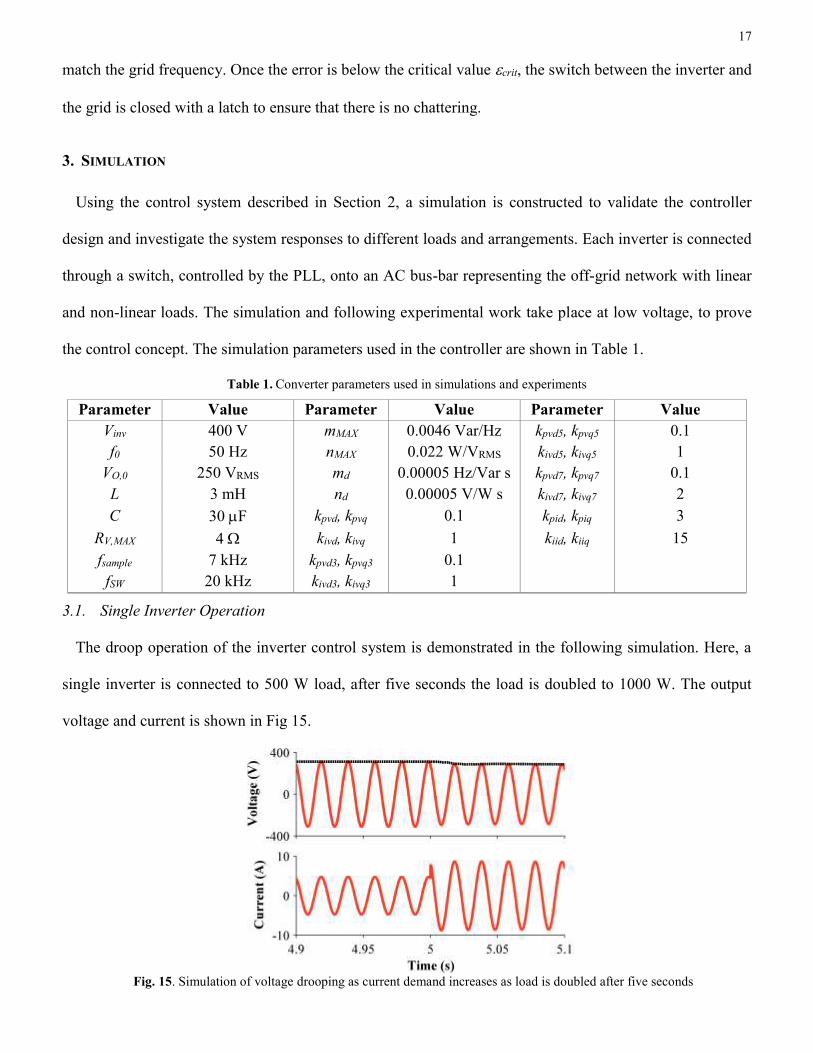
3.1. Single Inverter Operation

The droop operation of the inverter control system is demonstrated in the following simulation. Here, a

single inverter is connected to 500 W load, after five seconds the load is doubled to 1000 W. The output

voltage and current is shown in Fig 15.

Fig. 15. Simulation of voltage drooping as current demand increases as load is doubled after five seconds

18

This figure shows the voltage drooping as the current doubles, as is expected in the system.

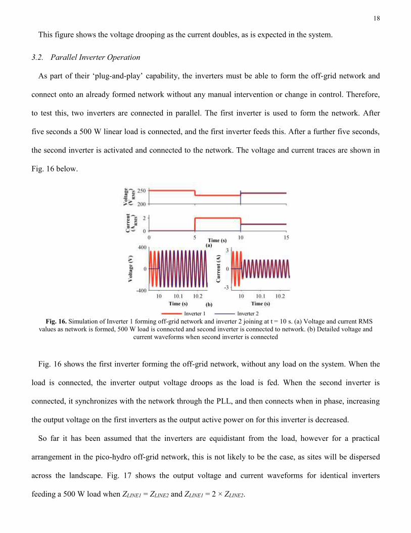
3.2. Parallel Inverter Operation

As part of their ‘plug-and-play’ capability, the inverters must be able to form the off-grid network and

connect onto an already formed network without any manual intervention or change in control. Therefore,

to test this, two inverters are connected in parallel. The first inverter is used to form the network. After

five seconds a 500 W linear load is connected, and the first inverter feeds this. After a further five seconds,

the second inverter is activated and connected to the network. The voltage and current traces are shown in

Fig. 16 below.

Fig. 16. Simulation of Inverter 1 forming off-grid network and inverter 2 joining at t = 10 s. (a) Voltage and current RMS

values as network is formed, 500 W load is connected and second inverter is connected to network. (b) Detailed voltage and

current waveforms when second inverter is connected

Fig. 16 shows the first inverter forming the off-grid network, without any load on the system. When the

load is connected, the inverter output voltage droops as the load is fed. When the second inverter is

connected, it synchronizes with the network through the PLL, and then connects when in phase, increasing

the output voltage on the first inverters as the output active power on for this inverter is decreased.

So far it has been assumed that the inverters are equidistant from the load, however for a practical

arrangement in the pico-hydro off-grid network, this is not likely to be the case, as sites will be dispersed

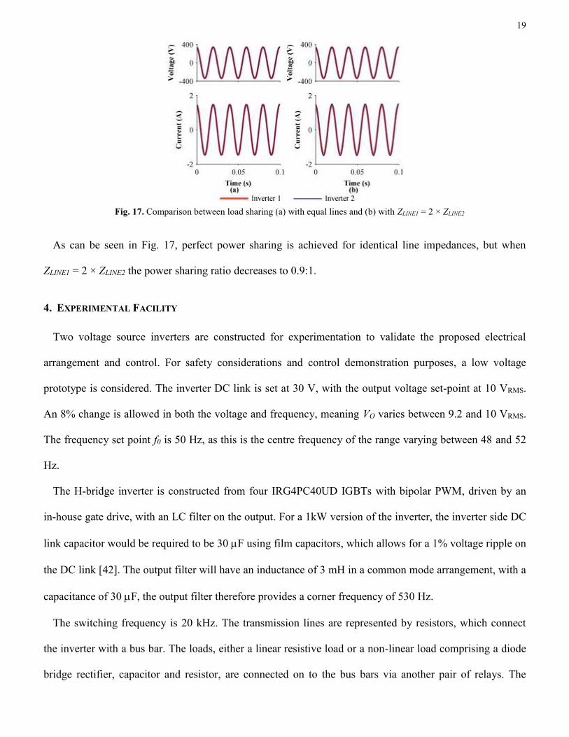
across the landscape. Fig. 17 shows the output voltage and current waveforms for identical inverters

feeding a 500 W load when ZLINE1 = ZLINE2 and ZLINE1 = 2 × ZLINE2.

19

Fig. 17. Comparison between load sharing (a) with equal lines and (b) with ZLINE1 = 2 × ZLINE2

As can be seen in Fig. 17, perfect power sharing is achieved for identical line impedances, but when

ZLINE1 = 2 × ZLINE2 the power sharing ratio decreases to 0.9:1.

4. EXPERIMENTAL FACILITY

Two voltage source inverters are constructed for experimentation to validate the proposed electrical

arrangement and control. For safety considerations and control demonstration purposes, a low voltage

prototype is considered. The inverter DC link is set at 30 V, with the output voltage set-point at 10 VRMS.

An 8% change is allowed in both the voltage and frequency, meaning VO varies between 9.2 and 10 VRMS.

The frequency set point f0 is 50 Hz, as this is the centre frequency of the range varying between 48 and 52

Hz.

The H-bridge inverter is constructed from four IRG4PC40UD IGBTs with bipolar PWM, driven by an

in-house gate drive, with an LC filter on the output. For a 1kW version of the inverter, the inverter side DC

link capacitor would be required to be 30 F using film capacitors, which allows for a 1% voltage ripple on

the DC link [42]. The output filter will have an inductance of 3 mH in a common mode arrangement, with a

capacitance of 30F, the output filter therefore provides a corner frequency of 530 Hz.

The switching frequency is 20 kHz. The transmission lines are represented by resistors, which connect

the inverter with a bus bar. The loads, either a linear resistive load or a non-linear load comprising a diode

bridge rectifier, capacitor and resistor, are connected on to the bus bars via another pair of relays. The

20

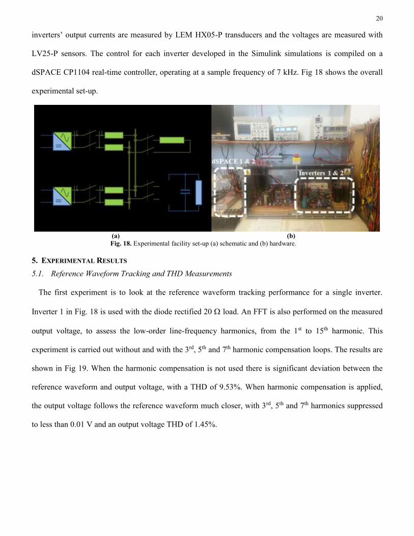
inverters’ output currents are measured by LEM HX05-P transducers and the voltages are measured with

LV25-P sensors. The control for each inverter developed in the Simulink simulations is compiled on a

dSPACE CP1104 real-time controller, operating at a sample frequency of 7 kHz. Fig 18 shows the overall

experimental set-up.

(a) (b) Fig. 18. Experimental facility set-up (a) schematic and (b) hardware.

5. EXPERIMENTAL RESULTS

5.1. Reference Waveform Tracking and THD Measurements

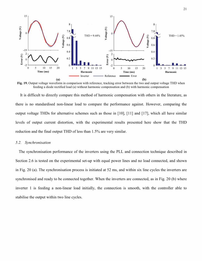
The first experiment is to look at the reference waveform tracking performance for a single inverter.

Inverter 1 in Fig. 18 is used with the diode rectified 20 load. An FFT is also performed on the measured

output voltage, to assess the low-order line-frequency harmonics, from the 1st to 15th harmonic. This

experiment is carried out without and with the 3rd, 5th and 7th harmonic compensation loops. The results are

shown in Fig 19. When the harmonic compensation is not used there is significant deviation between the

reference waveform and output voltage, with a THD of 9.53%. When harmonic compensation is applied,

the output voltage follows the reference waveform much closer, with 3rd, 5th and 7th harmonics suppressed

to less than 0.01 V and an output voltage THD of 1.45%.

21

(a) (b)

Fig. 19. Output voltage waveform in comparison with reference, tracking error between the two and output voltage THD when

feeding a diode rectified load (a) without harmonic compensation and (b) with harmonic compensation

It is difficult to directly compare this method of harmonic compensation with others in the literature, as

there is no standardised non-linear load to compare the performance against. However, comparing the

output voltage THDs for alternative schemes such as those in [10], [11] and [17], which all have similar

levels of output current distortion, with the experimental results presented here show that the THD

reduction and the final output THD of less than 1.5% are very similar.

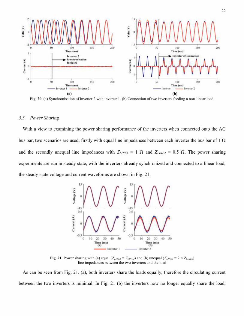
5.2. Synchronisation

The synchronisation performance of the inverters using the PLL and connection technique described in

Section 2.6 is tested on the experimental set-up with equal power lines and no load connected, and shown

in Fig. 20 (a). The synchronisation process is initiated at 52 ms, and within six line cycles the inverters are

synchronised and ready to be connected together. When the inverters are connected, as in Fig. 20 (b) where

inverter 1 is feeding a non-linear load initially, the connection is smooth, with the controller able to

stabilise the output within two line cycles.

22

(a) (b)

Fig. 20. (a) Synchronisation of inverter 2 with inverter 1. (b) Connection of two inverters feeding a non-linear load.

5.3. Power Sharing

With a view to examining the power sharing performance of the inverters when connected onto the AC

bus bar, two scenarios are used; firstly with equal line impedances between each inverter the bus bar of 1

and the secondly unequal line impedances with ZLINE1 = 1 and ZLINE2 = 0.5 . The power sharing

experiments are run in steady state, with the inverters already synchronized and connected to a linear load,

the steady-state voltage and current waveforms are shown in Fig. 21.

Fig. 21. Power sharing with (a) equal (ZLINE1 = ZLINE2) and (b) unequal (ZLINE1 = 2 × ZLINE2)

line impedances between the two inverters and the load

As can be seen from Fig. 21. (a), both inverters share the loads equally; therefore the circulating current

between the two inverters is minimal. In Fig. 21 (b) the inverters now no longer equally share the load,

23

even though they have the same power output potential. Inverter 2 takes a larger share of the current at a

ratio of 0.9:1, which matches the simulation in Section IV.

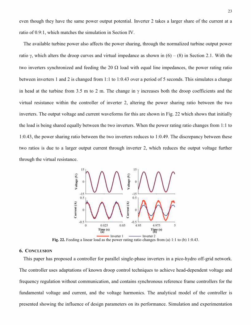
The available turbine power also affects the power sharing, through the normalized turbine output power

ratio , which alters the droop curves and virtual impedance as shown in (6) – (8) in Section 2.1. With the

two inverters synchronized and feeding the 20 load with equal line impedances, the power rating ratio

between inverters 1 and 2 is changed from 1:1 to 1:0.43 over a period of 5 seconds. This simulates a change

in head at the turbine from 3.5 m to 2 m. The change in increases both the droop coefficients and the

virtual resistance within the controller of inverter 2, altering the power sharing ratio between the two

inverters. The output voltage and current waveforms for this are shown in Fig. 22 which shows that initially

the load is being shared equally between the two inverters. When the power rating ratio changes from 1:1 to

1:0.43, the power sharing ratio between the two inverters reduces to 1:0.49. The discrepancy between these

two ratios is due to a larger output current through inverter 2, which reduces the output voltage further

through the virtual resistance.

Fig. 22. Feeding a linear load as the power rating ratio changes from (a) 1:1 to (b) 1:0.43.

6. CONCLUSION

This paper has proposed a controller for parallel single-phase inverters in a pico-hydro off-grid network.

The controller uses adaptations of known droop control techniques to achieve head-dependent voltage and

frequency regulation without communication, and contains synchronous reference frame controllers for the

fundamental voltage and current, and the voltage harmonics. The analytical model of the controller is

presented showing the influence of design parameters on its performance. Simulation and experimentation

24

demonstrate the effectiveness of the proposed methodology. The introduction of a synchronous reference

frame harmonic controller reduces the output voltage THD from 9.53% to 1.45%. The controller is also

shown to successfully form an off‑grid network, as well as synchronise to and support an already formed

network. When two inverters with equal input power are connected in parallel and the line impedances to

the load are identical, the units are able to equally share the load. If the line impedances are different, then

the power sharing ratio is no longer equal, reducing to 0.9:1 when the line impedances are at a ratio of 2:1.

When there is a difference in power rating between units, the units are able to share the load in proportion

to their respective ratings, for example, experiments showed that for a normalized turbine output power

ratio of 1:0.43, the power sharing ratio was 1:0.49. The simulations and experiments show that the

controller will be able to connect together a number of geographically-distant sources using only local

measurements to control the power output to form an off-grid network. The computational overhead for the

control algorithm is relatively high, requiring a fast processor and high sample frequency to operate the

system.

When the controller is implemented in a system, such as that illustrated in Fig. 1 with multiple sites at

varying heads using the same generation unit, there will be multiple generation and load nodes. All of these

nodes have the potential to vary, therefore matching supply and demand is a challenge. For a well-designed

pico-hydro system, the flow rate will be nearly constant, with changes happening over days and weeks,

therefore the supply can be considered reasonably constant. Therefore, the demand management of the

system is critical, requiring an in depth analysis of potential technical or social managerial solutions.

Further work in this project will include developing the complete power-electronic interface and carrying

out a system simulation, experimental testing with a 1 kW-scale variable flow turbine, and improving the

controller to reduce computational burden, as well as analysing the dynamic performance of the controller

in an off-grid network with multiple supply and load nodes.

APPENDIX

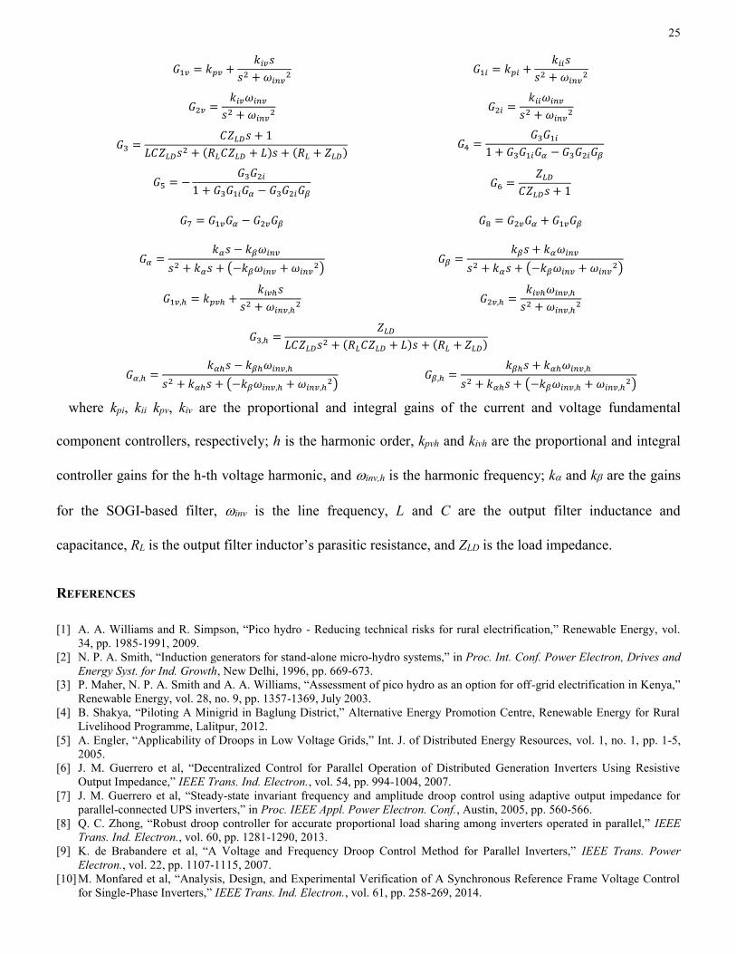
The symbols used in (14)-(16) are listed below:

25

𝐺1𝑣 = 𝑘𝑝𝑣 +𝑘𝑖𝑣𝑠

𝑠2 + 𝜔𝑖𝑛𝑣2 𝐺1𝑖 = 𝑘𝑝𝑖 +

𝑘𝑖𝑖𝑠

𝑠2 + 𝜔𝑖𝑛𝑣2

𝐺2𝑣 =𝑘𝑖𝑣𝜔𝑖𝑛𝑣

𝑠2 + 𝜔𝑖𝑛𝑣2 𝐺2𝑖 =

𝑘𝑖𝑖𝜔𝑖𝑛𝑣

𝑠2 + 𝜔𝑖𝑛𝑣2

𝐺3 =𝐶𝑍𝐿𝐷𝑠 + 1

𝐿𝐶𝑍𝐿𝐷𝑠2 + (𝑅𝐿𝐶𝑍𝐿𝐷 + 𝐿)𝑠 + (𝑅𝐿 + 𝑍𝐿𝐷) 𝐺4 =

𝐺3𝐺1𝑖

1 + 𝐺3𝐺1𝑖𝐺𝛼 − 𝐺3𝐺2𝑖𝐺𝛽

𝐺5 = −𝐺3𝐺2𝑖

1 + 𝐺3𝐺1𝑖𝐺𝛼 − 𝐺3𝐺2𝑖𝐺𝛽

𝐺6 =𝑍𝐿𝐷

𝐶𝑍𝐿𝐷𝑠 + 1

𝐺7 = 𝐺1𝑣𝐺𝛼 − 𝐺2𝑣𝐺𝛽 𝐺8 = 𝐺2𝑣𝐺𝛼 + 𝐺1𝑣𝐺𝛽

𝐺𝛼 =𝑘𝛼𝑠 − 𝑘𝛽𝜔𝑖𝑛𝑣

𝑠2 + 𝑘𝛼𝑠 + (−𝑘𝛽𝜔𝑖𝑛𝑣 + 𝜔𝑖𝑛𝑣2)

𝐺𝛽 =𝑘𝛽𝑠 + 𝑘𝛼𝜔𝑖𝑛𝑣

𝑠2 + 𝑘𝛼𝑠 + (−𝑘𝛽𝜔𝑖𝑛𝑣 + 𝜔𝑖𝑛𝑣2)

𝐺1𝑣,ℎ = 𝑘𝑝𝑣ℎ +𝑘𝑖𝑣ℎ𝑠

𝑠2 + 𝜔𝑖𝑛𝑣,ℎ2 𝐺2𝑣,ℎ =

𝑘𝑖𝑣ℎ𝜔𝑖𝑛𝑣,ℎ

𝑠2 + 𝜔𝑖𝑛𝑣,ℎ2

𝐺3,ℎ =𝑍𝐿𝐷

𝐿𝐶𝑍𝐿𝐷𝑠2 + (𝑅𝐿𝐶𝑍𝐿𝐷 + 𝐿)𝑠 + (𝑅𝐿 + 𝑍𝐿𝐷)

𝐺𝛼,ℎ =𝑘𝛼ℎ𝑠 − 𝑘𝛽ℎ𝜔𝑖𝑛𝑣,ℎ

𝑠2 + 𝑘𝛼ℎ𝑠 + (−𝑘𝛽𝜔𝑖𝑛𝑣,ℎ + 𝜔𝑖𝑛𝑣,ℎ2)

𝐺𝛽,ℎ =𝑘𝛽ℎ𝑠 + 𝑘𝛼ℎ𝜔𝑖𝑛𝑣,ℎ

𝑠2 + 𝑘𝛼ℎ𝑠 + (−𝑘𝛽𝜔𝑖𝑛𝑣,ℎ + 𝜔𝑖𝑛𝑣,ℎ2)

where kpi, kii kpv, kiv are the proportional and integral gains of the current and voltage fundamental

component controllers, respectively; h is the harmonic order, kpvh and kivh are the proportional and integral

controller gains for the h-th voltage harmonic, and inv,h is the harmonic frequency; k and k are the gains

for the SOGI-based filter, inv is the line frequency, L and C are the output filter inductance and

capacitance, RL is the output filter inductor’s parasitic resistance, and ZLD is the load impedance.

REFERENCES

[1] A. A. Williams and R. Simpson, “Pico hydro - Reducing technical risks for rural electrification,” Renewable Energy, vol.

34, pp. 1985-1991, 2009.

[2] N. P. A. Smith, “Induction generators for stand-alone micro-hydro systems,” in Proc. Int. Conf. Power Electron, Drives and

Energy Syst. for Ind. Growth, New Delhi, 1996, pp. 669-673.

[3] P. Maher, N. P. A. Smith and A. A. Williams, “Assessment of pico hydro as an option for off-grid electrification in Kenya,”

Renewable Energy, vol. 28, no. 9, pp. 1357-1369, July 2003.

[4] B. Shakya, “Piloting A Minigrid in Baglung District,” Alternative Energy Promotion Centre, Renewable Energy for Rural

Livelihood Programme, Lalitpur, 2012.

[5] A. Engler, “Applicability of Droops in Low Voltage Grids,” Int. J. of Distributed Energy Resources, vol. 1, no. 1, pp. 1-5,

2005.

[6] J. M. Guerrero et al, “Decentralized Control for Parallel Operation of Distributed Generation Inverters Using Resistive

Output Impedance,” IEEE Trans. Ind. Electron., vol. 54, pp. 994-1004, 2007.

[7] J. M. Guerrero et al, “Steady-state invariant frequency and amplitude droop control using adaptive output impedance for

parallel-connected UPS inverters,” in Proc. IEEE Appl. Power Electron. Conf., Austin, 2005, pp. 560-566.

[8] Q. C. Zhong, “Robust droop controller for accurate proportional load sharing among inverters operated in parallel,” IEEE

Trans. Ind. Electron., vol. 60, pp. 1281-1290, 2013.

[9] K. de Brabandere et al, “A Voltage and Frequency Droop Control Method for Parallel Inverters,” IEEE Trans. Power

Electron., vol. 22, pp. 1107-1115, 2007.

[10] M. Monfared et al, “Analysis, Design, and Experimental Verification of A Synchronous Reference Frame Voltage Control

for Single-Phase Inverters,” IEEE Trans. Ind. Electron., vol. 61, pp. 258-269, 2014.

26

[11] A. Micallef et al, “Reactive power sharing and voltage harmonic distortion compensation of droop controlled single phase

islanded microgrids”, IEEE Trans. Smart Grid, vol. 5, pp. 1149-1158, 2014.

[12] M. N. Marwali, J. Jung, A. Keyhani, “Control of Distributed Generation Systems – Part II: Load Sharing Control”, IEEE

Trans. Power Electron., vol. 19, pp. 1551-1531, 2004.

[13] Q. C. Zhong and G. Weiss, “Synchronverters: Inverters That Mimic Synchronous Generators”, IEEE Trans. Ind. Electron.,

vol. 58, pp. 1259-1267, 2011.

[14] H. P. Beck and R. Hesse, “Virtual synchronous machine”, in Proc. 9th Int. Conf. Elect. Power Quality and Utilisation,

Barcelona, 2007, pp. 1-6.

[15] Q. C. Zhong and T. Hornik, Control of Power Inverters in Renewable Energy and Smart Grid Integration, Chichester: John

Wiley & Sons Ltd, 2013, Chap. 2.

[16] S. J. Chiang and J. M. Chang “Parallel operation of series-connected PWM voltage regulators without control

interconnection”, IEE Proc. Electric Power Appl., vol. 148, pp. 141-147, 2001.

[17] Q. C. Zhong, “Harmonic Droop Controller to Reduce the Voltage Harmonics of Inverters,” IEEE Trans. Ind. Electron., vol.

60, pp. 936-945, 2013.

[18] M. Ciobotaru et al, “A New Single-Phase PLL Structure Based on Second Order Generalised Integrator,” in Proc. IEEE

Power Electron. Specialists Conf., Jeju, 2006, pp. 1-6.

[19] Q. C. Zhong and Y. Zeng, “Parallel Operation of Inverters with Different Types of Output Impedance”, in Proc. IEEE Ind.

Electon. Conf., Vienna, 2013, pp. 1398-1403.

[20] S. J. Williamson, B. H. Stark and J. D. Booker, “Performance of a low-head pico-hydro Turgo turbine,” Applied Energy,

vol. 102, pp. 1114-1126, 2013.

[21] J. L. Márqueza, M. G. Molinab, and J. M. Pacasc, “Dynamic modeling, simulation and control design of an advanced micro-

hydro power plant for distributed generation applications,” International Journal of Hydrogen Energy, vol. 35, pp. 5772–

5777, 2010

[22] G. Muller and J. Senior, “Simplified theory of Archimedean screws,” Journal of Hydraulic Research, vol. 47, pp. 666–669,

2009.

[23] S. J. Williamson, B. H. Stark and J. D. Booker, “Low head pico hydro turbine selection using a multi-criteria analysis,”

Renewable Energy, vol. 61, pp 43-50, 2014.

[24] A. Roshan et al, “A D-Q Frame Controller for a Full-Bridge Single Phase Inverter Used in Small Distributed Power

Generation Systems,” in Proc. IEEE Appl. Power Electron. Conf., Anaheim, 2007, pp. 641-647.

[25] B. Burger and A. Engler, “Fast Signal Conditioning in Single Phase Systems,” in Proc. European Power Electron. and

Drives Conf., Graz, 2001.

[26] K. de Brabandere et al, “Design and Operation of a Phase-Locked Loop with Kalman Estimator-Based Filter for Single-

Phase Applications,” in Proc. IEEE Conf. on Ind. Electron., Paris, 2006, pp. 525-530.

[27] C. A. Busada, S. Gómez Jorge, A. E. Leon, and J. A. Solsona, “Current Controller Based on Reduced Order Generalized

Integrators for Distributed Generation Systems,” IEEE Trans. Ind. Electron., vol. 59, pp. 2898-2909, 2012.

[28] M. Liserre , R. Teodorescu and F. Blaabjerg "Multiple harmonics control for three-phase grid converter systems with the

use of PI-RES current controller in a rotating frame", IEEE Trans. Power Electron., vol. 21, pp.836 -841 2006.

[29] C. Lascu , L. Asiminoaei , I. Boldea and F. Blaabjerg "Frequency response analysis of current controllers for selective

harmonic compensation in active power filters", IEEE Trans. Ind. Electron., vol. 56, pp.337 -347, 2009.

[30] R. Zhang et al, “A grid simulator with control of single-phase power converters in D-Q rotating frame,” in Proc IEEE Annu.

Power Electron. Specialists Conf., Cairns, 2002, pp. 1431-1436.

[31] M. Karimi-Ghartemani, “Universal Integrated Synchronization and Control for Single Phase DC/AC Converters”, IEEE

Trans. Power Electron., in press, DOI 10.1109/TPEL.2014.2304459

[32] B. Bahrani, et al, "A Multivariable Design Methodology for Voltage Control of a Single-DG-Unit Microgrid", IEEE Trans.

Ind. Informat., vol. 9, pp. 589-599, 2013.

[33] B. Bahrani , A. Rufer , S. Kenzelmann and L. Lopes "Vector control of single-phase voltage source converters based on

fictive axis emulation", IEEE Trans. Ind. Appl., vol. 47, pp.831-840, 2011.

[34] D. N. Zmood and D. G. Holmes, “Stationary Frame Current Regulation of PWM Inverters With Zero Steady-State Error,”

IEEE Trans. Power Electron., vol. 18, pp. 814-822, 2003.

[35] P. Mattavelli, “A closed-loop selective harmonic compensation for active filters”, IEEE Trans. Ind. Appl., vol. 37, pp. 81-89,

2001.

[36] Y. Xiaoming, W. Merk, H. Stemmler, J. Allmeling, “Stationary-frame generalized integrators for current control of active

power filters with zero steady-state error for current harmonics of concern under unbalanced and distorted operating

conditions”, IEEE Trans. Ind. Appl., vol.38, pp. 523-532, 2002.

[37] S. Golestan, M. Monfared, F. D. Freijedo, J. M. Guerrero, "Dynamics Assessment of Advanced Single-Phase PLL

Structures,” IEEE Trans. Ind. Electron., vol. 60, pp. 2167-2177, 2013.

[38] S. Golestan, M. Monfared, F. D. Freijedo, J. M. Guerrero, "Advantages and Challenges of a Type-3 PLL," IEEE Trans.

Power Electron., vol. 28, pp. 4985-4997, 2013.

[39] H. Geng; J. Sun; S. Xiao; G. Yang "Modeling and Implementation of an All Digital Phase-Locked-Loop for Grid-Voltage

Phase Detection", IEEE Trans. Ind. Informat., vol. 9 pp. 772-780, 2013.

27

[40] P. Rodriguez , A. Luna , I. Candela , R. Mujal , R. Teodorescu and F. Blaabjerg "Multiresonant frequency-locked loop for

grid synchronization of power converters under distorted grid conditions", IEEE Trans. Ind. Electron., vol. 58, pp. 127-

138, 2011.

[41] J. M. Guerrero, J. C. Vasquez, J. Matas, L. G. de Vicuna, M. Castilla, “Hierarchical Control of Droop-Controlled AC and

DC Microgrids—A General Approach Toward Standardization”, IEEE Trans. Ind. Electron., vol. 58, pp. 158-172, 2011.

[42] M. Salcone and J. Bond, “Selecting film bus link capacitors for high performance inverter applications,” in Proc. Int.

Electric Machines and Drives Conf., Miami, 2009, pp. 1692–1699