Embed Size (px)
Citation preview

1
Impacts of Environmental Muck Dredging 2016-2017
Wind and microclimate analysis for improved
site characterization in support of
environmental flow modeling (Subtask 7)
Final Project Report Submitted to
Brevard County Natural Resources Management Department
2725 Judge Fran Jamieson Way, Building A, Room 219
Viera, Florida 32940
Funding provided by the Florida legislature as part of
DEP Grant Agreement No. S0714 – Brevard County Muck Dredging
Principal Investigator: Dr. Steven M. Lazarus1
Indian River Lagoon Research Institute
150 West University Boulevard
Florida Institute of Technology
Melbourne, FL 32901
FINAL
November 2017
1 Contact information email: [email protected]; office phone: 321-394-2160.

i
Table of Contents Page
i. List of Figures…………..…………………………….………………………...….......... ii
ii. List of Tables..………………….………………………..….……………...………........ iv
iii. Acknowledgements………………………………...………………………..…............... v
iv. Plain English Summary…………………………………………………………………. vi
v. Technical Abstract……………………………………………………………..…………1
vi. Introduction…………………………………………………………….......…………… 4
1. Detailed analysis of the microclimate of the mouth of Turkey Creek…............................. 5
i. Approach ……………….……………………………………................................ 5
ii. Results and Discussion…………………………..………………………….…...... 7
1.1. Fetch Analysis ………………………………………………………..…….. 7
1.2 Synoptic Pattern and Water Temperatures: 11 March 2017........................... 8
1.3 Comparison of FIT lidar, Kestrel, and Remote ASOS………………...……. 10
1.4 Roving versus Stationary Kestrel……………..………………………….…. 12
1.5 Vertical Profiles: Structure and Evolution of the Surface Layer……………. 13
1.6 Wind Direction and Fetch……………..………………………….…............. 19
2. Site Characterization………………………………….…………........................................ 23
i. Approach…………………………………………………………..………………. 23
ii. Results and Discussion……………………..……………………………............... 24
2.1. Vero Beach (KVRB)………………………………………………………… 24
2.2 Fort Pierce (KFPR).………………………………………………………..... 28
2.3 Melbourne (KMLB) ………………………………………………………… 32
3. Wind Forcing Time Series …………………………………..………................................. 36
i. Approach …….……………………………………................................................. 36
ii. Results and Discussion……………………..……………………………............... 38
3.1 Weibull fit of the WRF Wind Speed Distributions …………………………. 38
3.2 ASOS to ‘Water Friendly’ Regressions …………………………………...... 41
3.3 Extension of Weibull fit to higher wind speeds……………………………... 45
3.4 Synthetic Time Series + Uncertainty: November 2013…………………….... 46
4. Deliverables…………………………………………………………………..................... 49
5. References…………………………………………………………………........................ 49
6. Appendices………………………………………..………………………......................... 51
A: WRF wind speed probability distributions………………………………….….…….... 51
B: KMLB/XRPT regression coefficients: All wind directions (2013-2015)……………... 52
C: KMLB/XRPT regression coefficients: Open fetch wind directions (2013-2015)……... 53
D: Enlarged histograms from Fig. 3.8…………………………………………………...... 54

Impacts of Environmental Muck Dredging at Florida Institute of Technology 2016-2017, Final Report, November 4, 2017
ii
i. List of Figures
Fig. # Description Page
1.1 Palm Bay lidar (on 11 March 2017) and ASOS wind speed measurement locations 6
1.2 NLCD land use data (2011) and lidar based fetch rays, Palm Bay 7
11 March 2017
1.3 Palm Bay lidar-based fetch analysis and NLCD land use 8
1.4 Palm Bay lidar-based fetch analysis, satellite view 8
1.5 Water Temperature, Ocean Research and Conservation Association 9
KILROY: Turkey Creek 2
1.6 RAP wind speed, NAM sea level pressure and surface winds 18 UTC 9
11 March 2017
1.7 Directional roughness (m) estimates for regional ASOS and WeatherFlow stations 11
1.8 View looking north at the KFPR ASOS 12
1.9 Lidar wind speed profiles, 15–20 UTC 11 March 2017 14
1.10 Lidar wind direction profiles, 15–20 UTC 11 March 2017 14
1.11 30-min average lidar wind profiles at Palm Bay 11 March 2017 15
1.12 Lidar turbulence intensity profiles, 15–20 UTC 11 March 2017 15
1.13 Wind speed at KMLB, KVRB, KFPR (gray line), lidar and Kestrels (Palm Bay) 17
11 March 2017
1.14 Kestrel wind speed differences at the six sites in Palm Bay, 11 March 2017 18
1.15 Lidar 11 m wind direction, 11 March 2107 (Palm Bay) 18
1.16 Lidar wind speed at 11 m and 100 m, Palm Bay 11 March 2017 19
1.17 Lidar 100 m-to-11 m wind speed ratio versus wind direction, Palm Bay 20
11 March 2017
1.18 Lidar 100 m-to-11 m wind speed ratio versus fetch length, Palm Bay 21
11 March 2017
1.19 Lidar 11 m turbulence intensity versus the average wind direction, Palm Bay 22
11 March 2017
1.20 Lidar 11 m turbulence intensity and wind direction time series, Palm Bay 22
11 March 2017
1.21 Lidar 100 m-to-11 m wind speed ratio versus turbulence intensity, Palm Bay 23
11 March 2017
2.1 KVRB ASOS and lidar wind roses, 25 March–6 April 2017 25
2.2 KVRB lidar 100 m-to-11 m wind speed ratios, 25 March–6 April 2017 26
2.3 KVRB ASOS three-year (2014-2016) gustiness climatology 27
2.4 KVRB roughness versus the climatological (2014-2016) ASOS gust factor. 27
2.5 KVRB ASOS three-year (2014-2016) wind rose 28
2.6 KFPR ASOS and lidar wind roses for 8 April–30 April 2017 29
2.7 KFPR lidar 100 m-to-11 m wind speed ratios for 8 April–30 April 2017 29

Impacts of Environmental Muck Dredging at Florida Institute of Technology 2016-2017, Final Report, November 4, 2017
iii
Fig. # Description Page
2.8 KFPR ASOS three-year (2014-2016) gustiness climatology 30
2.9 KFPR roughness versus the climatological (2014-2016) ASOS gust factor 31
2.10 KFPR ASOS ultrasonic anemometer and glide slope 31
2.11 KFPR ASOS three-year (2014-2016) wind rose 32
2.12 FIT lidar (looking SW) at the Melbourne International Airport 32
2.13 KMLB ASOS and lidar wind roses for 21 January–27 January 2017 33
2.14 KMLB lidar 100 m-to-11 m wind speed ratios for 21 January–27 January 2017 34
2.15 KMLB ASOS three-year (2014-2016) gustiness climatology 34
2.16 KMLB (and KVRB, KFPR) roughness versus the climatological (2014-2016) 35
ASOS gust factor
2.17 KMLB ASOS three-year (2014-2016) wind rose 35
3.1 Environmental model subdomains and WRF water points within 36
Banana River shape file.
3.2 WRF domain and wind speed from the 80º/15 m/s simulation 37
3.3 WRF density wind speed histograms, PDF fits, and Q-Q plots: 39
Banana River domain
3.4 Weibull variance versus WRF average wind speed: Banana River subdomain 40
3.5 Weibull variance versus WRF wind direction: Banana River subdomain 40
3.6 Weibull scale parameter versus average wind speed: Banana River subdomain. 41
3.7 Wind speed histograms (Jan 2013—May 2016) for six WeatherFlow sites 42
3.8 KMLB ASOS, WeatherFlow XRPT station locations and regression, 42
November 2013
3.9 Regression statistics (XRPT versus KMLB) by month for 2013-2015 44
3.10 Scatterplots of wind speed for = 0.05 regression, November 2013 45
3.11 Wind speed box plots for XRPT and synthetic time series, November 2013 47
3.12 Wind speed time series for KMLB, synthetic (with spread), and XRPT 48
November 2013
3.13 Wind speed time series for KMLB, synthetic (with spread), and XRPT 48
13-16 November 2013

Impacts of Environmental Muck Dredging at Florida Institute of Technology 2016-2017, Final Report, November 4, 2017
iv
ii. List of Tables
Table Description Page
1.1 ASOS station locations, ID, and name 10
1.2 WxFlow directional roughness estimates (m) for three ASOS locations 11
1.3 Palm Bay wind speed statistics for 11 March 2017: Lidar versus ASOS 12
1.4 Palm Bay wind speed statistics for 11 March 2017: Kestrel 13
1.5 Palm Bay least-squares coefficients for lidar wind profiles, 11 March 2017 16
1.6 Palm Bay IBL height (m) estimates 17
2.1 Observation counts for three ASOS wind roses: KVRB, KFPR, and KMLB 24
2.2 KVRB ASOS versus lidar wind statistics, 25 March–6 April 2017 25
2.3 KFPR ASOS versus lidar wind statistics, 8 April–30 April 2017 28
3.1 Error statistics for 10 synthetic wind speed time series realizations, 44
November 2013
3.2 Wind speed standard deviations at XRPT, KMLB, and synthetic data, 46
November 2013
A.1 Regression coefficients for XRPT versus KMLB, all wind directions 51
(2013-2015)
B.1 Regression coefficients for XRPT versus KMLB, open fetch directions 52
(2013-2015)

Impacts of Environmental Muck Dredging at Florida Institute of Technology 2016-2017, Final Report, November 4, 2017
v
iii. Acknowledgements
The research presented herein reflects the nexus of three separate projects. The primary support
($86K) comes from the state of Florida via DEP Grant Agreement No. S0714 – Brevard County
Muck Dredging. Indirect support from NOAA CSTAR award number NA14NWS4680014, An
Ensemble-based Approach to Forecasting Surf, Set-Up and Surge in the Coastal Zone ($367K) in
the form of WRF model simulations from Ph. D student Bryan Holman and an internally funded
(Florida Institute of Technology) equipment award Lidar Measurements of the Low-Level Wind
Profile on the IRL ($151K). The PI would like to thank both Mike Splitt (FIT faculty, College of
Aeronautics) and graduate student Vanessa Haley (Department of Ocean Engineering and
Science). Professor Splitt provided a significant amount of in-house and in-the-field lidar support
for the site characterizations while Ms. Haley contributed to both field deployment efforts as well
as the research associated with the generation of the wind forcing (section 3 of this report). The
funding from this project has provided both stipend and tuition for the graduate research that
comprises her Masters work. I would also like to thank WeatherFlow Inc. for providing some of
the observation data used in this research.
Impacts of Environmental Muck Dredging at Florida Institute of Technology 2016-2017, Final Report, November 4, 2017
vi
iv. Plain English Summary
The primary purpose of the study is to provide an empirical description of the IRL wind field
(and its variability) for modeling purposes. Toward that end, we develop an algorithm that relates
airport meteorological station data to site-specific (lagoon) wind measurements. In part, this
allows airport station data to be used in the calibration and verification of the Zarillo
hydrodynamic/sediment transport model in lieu of costly, site-specific wind measurements. In
support of this effort, we conducted 1) a detailed wind microclimate analysis of the Palm Bay
dredge site and, 2) a wind-related site characterization for three National Weather Service
locations. The meteorological role as it relates to (IRL) muck intersects a broad range of
environmental related issues including re-suspension, erosion, transport (i.e., advection), turbulent
mixing, runoff (hydrology), algal blooms, etc.
Approximately 6 weeks of fieldwork were conducted in which the FIT wind lidar was
deployed. There were extended site visits to nearby National Weather Service Automated Surface
Observing System (ASOS) stations as well as a day visit to the dredge site in Palm Bay. The three
ASOS site assesments/lidar visits address the QA requirements of this work (lidar wind
validation), and help address ASOS siting issues – which is important given that these sites are
used to develop the wind forcing. The Ft. Pierce ASOS appears to be an outlier due to blocking
issues (and a lower measurement height) and thus data from this site were not used to generate the
synthetic wind forcing. Results from the microclimate analysis indicate relatively large variability
in wind speeds within Palm Bay (as much as 10 kt) – large enough to impact flow modeling.
Using a wind gust approach, an assessment of published roughness estimates at the three ASOS
sites was performed. Results for both the Ft. Pierce and Vero Beach ASOS were consistent with
existing reports, but degraded for Melbourne. Our analysis indicates that, for some flow
directions, the published roughness estimates at the Melbourne ASOS are too low. This
underscores the problematic nature of accurately determining low end roughness values – a
potential issue if one chooses to adjust (from land to water) the ASOS wind observations using
this type of method.
To address the essential question of this funded work, “What is the wind over the lagoon?”, a
statistical approach is applied to model and observed winds to create a synthetic wind forcing time
series along with an estimate of its variability (spread). These winds are generated by regressing
observations at ASOS locations against in-situ water friendly sites, while the spread is obtained
from repeated sampling of the spatial variability from 180 Weather Research and Forecast (WRF)
model simulations where the wind speed and direction were systematically varied. This approach
is designed to provide a water representative estimate of the wind speed as well as a measure of it
representativeness. The synthetic wind forcing has been applied to the FIT Coastal Modeling
System to assess both the impact and sensitivity of the model, in particular the sediment loading,
to uncertainty in the wind-driven circulation.

1
Wind and microclimate analysis for improved site characterization in support of environmental
flow modeling (Subtask 7).
Dr. Steven M. Lazarus, Florida Institute of Technology
v. Technical Abstract The primary purpose of the study is to provide an empirical description of the IRL wind field (and
its variability) for modeling purposes. Toward that end, we develop an algorithm that relates
airport meteorological station data to site-specific (lagoon) wind measurements. In part, this
allows airport station data to be used in the calibration/verification of the Zarillo
hydrodynamic/sediment transport model without necessarily collecting costly, site-specific wind
measurements. In support of this effort, we conduct a detailed wind microclimate analysis of the
Palm Bay dredge site and a wind-related site characterization for three National Weather Service
locations. The meteorological role as it relates to (IRL) muck intersects a broad range of
environmental related issues including re-suspension, erosion, transport (i.e., advection), turbulent
mixing, runoff (hydrology), algal blooms, etc. IRL muck remains an ongoing problem –
threatening the future of the lagoon. While its removal is of paramount importance, a better
understanding of the various contributing and exacerbating factors is also beneficial for
management and planning.
Approximately 6 weeks of field work were conducted in which the FIT wind lidar (ZephIR 300)
was deployed. There were extended site visits to nearby National Weather Service Automated
Surface Observing System (ASOS) stations in Melbourne (KMLB), Vero Beach (KVRB) and Ft.
Pierce (KFPR). Additional single day deployments, on the IRL, were also carried out for Tropical
Storm Hermine and Hurricane Matthew as well as at the dredge site in Palm Bay. The Palm Bay
field work includes a fetch2 analysis that incorporates high resolution land use to assess the air
flow through the Palm Bay “gap” (i.e., opening) during an onshore flow wind event on 11 March
2017. Variation in fetch, based on the lidar location, ranged from 300 m to 3500 m depending on
the wind direction. The wind sampling methodology, which included both moving and stationary
instruments, provided a means by which the winds can be directly compared throughout the
sampling interval. Despite the fetch favorable flow (from the northeast), wind speed differences
along the west edge the bay were relatively small (+/- 2 knots, hereafter kt). However, at the mouth
of the bay (Castaway Park Pier), wind speeds were on the order of 4 kt higher than observed at the
lidar – suggesting that the impact of the upstream land roughness can be important. Different
proxies for surface roughness including turbulence intensity3, the ratio of the lidar wind speeds at
heights of 100 m and 11 m (above ground level), and wind speed profiles were each examined.
Results were consistent across each of these surface roughness-related parameters with decreasing
2 Fetch is defined here as the ‘unobstructed’ total distance travelled by airflow while over water only. 3 Turbulence intensity is the ratio of the standard deviation of the wind speed divided by the mean (over a defined
time interval). It is often used to characterize the surface roughness at an observation site.

Impacts of Environmental Muck Dredging at Florida Institute of Technology 2016-2017, Final Report, November 4, 2017
2
ratios for increasing fetch, decreasing atmospheric turbulence with height, and a multilayer wind
profile comprised of an internal boundary layer associated with the rough-to-smooth transition
downwind of Castaway Park.
To quantify the impact of the roughness transition upstream of the lidar at Palm Bay, the wind
ratio was regressed against both wind direction and fetch. It is difficult to fully resolve the
significant changes in the wind speed that occur for fetch lengths on the order of 350 m (i.e., within
the bay fetch). This is shown to be related to the large increase (order of magnitude) in the fetch
length through the ‘gap’ of the bay and wind direction variability. A simple inexpensive fetch
dependent equation is derived. This simple model could be used to create a high resolution gridded
surface wind analysis (within the bay) given 100 m wind speed and direction (e.g., from model
output). This type of microclimate wind analysis would likely prove beneficial to flow modeling,
erosion studies, etc.
While the three site assesments/lidar visits were relatively short, ranging from 1-3 week
deployments, they are useful as they address the QA requirements of this work. Composite
statistics, including wind roses, gustiness roses and histograms, at each of the ASOS locations are
also provided and compared against published roughness estimates. At both Vero Beach and Fort
Pierce, where the lidar was sited within 30 meters of the ASOS, the QA metrics (roses, statistics)
indicate good agreement. Our siting near the FIT aviation facility at Melbourne precludes a direct
assessment / comparison of 10 m winds, however analysis of the 100 m winds compare favorably
to the KMLB ASOS and suggest that the flow at that level is, for the most part, undisturbed and
above the impact of the nearby surface elements.
Of the three ASOS sites, KFPR appears to be an outlier. In general, the peak wind speeds for most
directions are lower at KFPR and occur less frequently. In addition to being weaker, northerly
flow is also observed slightly less often at KFPR (due to land cover/forest). However, the southerly
and southwesterly flow also appears to be somewhat muted (i.e., less frequent) compared to KVRB
and KMLB. Having a well-behaved (i.e., representative) baseline wind is important with respect
to the regression approach used here to provide an estimate of the IRL flow.
Using a 3-year gustiness climatology, an assessment of published roughness estimates at the three
sites is presented. The relationship between the roughness and gustiness is quite good for both
KFPR and KVRB, but degraded (low correlation) for KMLB due to the low dynamic range. We
also perform a regression for all three sites combined. The R2 is reltively high at 0.64, and reveals
a small cluster of outliers associated with low roughness values (all but of one of which are from
KMLB. Our gustiness analysis indicates that the published roughness estimates from these
directions are likely too low and underscores the problematic nature of accurately determining the
small surface roughness values in general. This is an issue if one chooses to standardize
observations to an open fetch (i.e., the upstream flow direction is water) using roughness.

Impacts of Environmental Muck Dredging at Florida Institute of Technology 2016-2017, Final Report, November 4, 2017
3
To address the essential question of this funded work, i.e., “What is the wind over the lagoon?”, a
statistical approach is applied to both model and observed winds to create a synthetic wind forcing
time series along with an estimate of its variability for use in the FIT Coastal Modeling System
(CMS). In order to accomplish this, we pair an ASOS with a nearby WeatherFlow station for each
of the 6 CMS subdomains ranging from New Smyrna (Volusia Co.) south to Ft. Pierce (St. Lucie
Co). The methodology is illustrated using one of the CMS domains (Banana River) for which a
least-squares approach is applied to generate monthly regression equations between the observed
wind speed at KMLB versus that of a water representative lagoon station at Rocky Point (XRPT)
for a 3-year period. In part, the purpose of the monthly regressions is to indirectly account for the
impact of seasonal variations in the relationship between the winds at the two locations (e.g.,
changes in static stability4). Regardless of the time of year, the winds are consistently higher at
XRPT than KMLB – with larger differences for higher wind speeds. The monthly regression
coefficients are used to map the winds from KMLB (the predictor) to the wind friendly location,
XRPT (the predictand). While wind speed from XRPT could be used directly here, the regression
methodology provides a means by which a lagoon-based wind estimate can be obtained from the
wind at KMLB – even if the XRPT observation is missing or not available (note that the
WeatherFlow data are proprietary). The scatter in the monthly regressions (i.e., standard error) is
used to add Gaussian noise to the regressed wind speed (i.e. synthetic wind speed = regression
wind speed + noise).
The regressed wind speeds are used to develop an uncertainty estimate (1 standard deviation) that
is obtained from the spatial variability within 180 Weather Research and Forecast (WRF) model
simulations in which the wind speed and direction were systematically varied (10 wind speed bins
and 18 cardinal directions). Despite the large number of WRF simulations, they do not cover the
full range of observed winds (these simulations were generated as part of a separate project).
Hence, instead of sampling the WRF wind speed distributions directly to estimate the spread, a
Weibull5 fit is performed for each of the 180 wind speed/direction distributions within the Banana
River domain. The fit yields (180) estimates for each of the two free parameters (i.e., the variance
and shape factor). The Weibull parameters are then regressed (independently) against the average
model wind speed within the Banana River domain and used to extend the range of the simulated
wind speeds. The regressed (i.e., synthetic) wind speed, along with the ASOS wind direction,
determines the relevant Weibull distribution from which to sample. 1000 samples/per observation
are generated and make up the spread associated with each synthetic observation.
A comparison of the time series indicates that the methodology preserves the mean of the
observations – i.e., no bias between XRPT and the synthetic observations. The standard deviation
4 Atmospheric static stability is related to the vertical temperature profile and can be approximated by air / water
differences with stable (unstable) having air temperatures warmer (cooler) than the water. Changes in stability impact
the surface air flow. 5 The Weibull is a probability distribution function that is commonly used to fit (i.e., estimate) wind speed distributions
for wind energy purposes. The distribution depends on two parameters, scale (height) and shape (slope).

Impacts of Environmental Muck Dredging at Florida Institute of Technology 2016-2017, Final Report, November 4, 2017
4
of the synthetic data falls between the two observations (KMLB and XRPT) used in the regression.
Furthermore, approximately 40% of the observations (XRPT) fall within the model generated
spread – with an equal number greater/less than the envelope. The framework allows for additional
variability and, if desired, the procedure could be tuned to ensure that the standard deviation of the
synthetic data matches that of the water representative observation (in this case, XRPT).
Assuming that the model variability captures that the observed (true) variability over the IRL, this
approach provides both a water representative estimate of the wind speed and a unique measure of
uncertainty. The latter is designed expressly to provide a means by which ensemble6 wind forcing
time series can be generated by repeated sampling of the statistical distributions (i.e., the wind
speed spread) as defined by the WRF. The ensemble (multiple) wind forcing time series are
currently being used, within the environmental flow model, to assess the impact and sensitivity of
the model response as it relates to water level, flow, and sediment suspension.
vi. Introduction The impact of wind forcing on estuaries in general has been documented in various studies (e.g.,
Pitts, 1989; Frazel, 2009; Rohweder et al., 2012). While recognized as an important component
of a highly integrated ecosystem, the Indian River Lagoon wind field is not well observed. While
longer term climatologies exist as part of the Automated Surface Observing System (ASOS), these
‘gold standard’ stations are generally sited at airports and the degree in which they represent the
winds around water bodies is not clear. However, there are a number of different ways to ‘map’
winds from observation locations to data free regions some of which require both model and
observations or knowledge of the surface roughness. At a height of 10 m, most small scale wind
variability arises from surface roughness elements (i.e., land cover or land use). In this case, the
typical assumptions are that the local wind variability disappears at the top of the surface layer
(often taken to be 60 m height, e.g., Verkaik et al., 2006). In general, the surface ‘footprint’ (i.e.,
the upwind elements that affect the observed 10 m wind) extends only a few hundred meters
upstream while higher up, the upwind footprint increases in size. The 10 m wind can be brought
up to what is referred to as the ‘blending height’ (i.e., the height at which the impact of the local
surface elements is minimal) if the observed roughness is known and the log-law7 is applicable
(turbulent flow). This ‘free’ atmospheric wind can then be brought back down (to 10 m) using a
different roughness (e.g., open water). Hence, one obvious benefit of site characterization is that
the wind at an observation location can then be used to infer the flow at another (proximity)
location without a meteorological station – provided the surface roughness is known reasonably
well at both sites. If the remote site has an open fetch (e.g., water point) – it may be reasonable to
map winds at these locations by assigning an over-water roughness. However, for other scenarios
such as heterogeneous surroundings and/or stable thermal stratification, this process is generally
6 One type of ensemble (described herein) is the creation of multiple simulations from a single model – each of which
have been generated from different forcing (wind speed in this case). 7 Also known as the ‘law of the wall’, assumes that the velocity between a point in the turbulent flow and the wall is
a logarithmic function of the distance from the boundary (see https://en.wikipedia.org/wiki/Law_of_the_wall).
Impacts of Environmental Muck Dredging at Florida Institute of Technology 2016-2017, Final Report, November 4, 2017
5
more complicated. As an alternative approach, data assimilation combines both model and
observations in order to spread information from data rich regions to data poor. These techniques
range in levels of sophistication – and can be computationally expensive, especially at high spatial
resolution. There are also a host of statistical downscaling techniques, in which some physical
attribute such as a land / water mask, land use, fetch can be used to infer the subscale behavior
from coarser resolution model output. In this case, observations are typically used to correct for
bias in the model output (Holman et al., in review) prior to downscaling and a ‘training’ (prior)
data set may be needed in order to develop statistically meaningful relationships (e.g., fetch
length).
The main purpose of this study is to develop lagoon representative wind forcing to better predict
muck re-suspension and transport in the CMS8. Because the environmental flow model forcing is
derived from a single time series forcing – a gridded wind field unnecessary for the purposes of
this work. Hence, a roughness based approach (as originally proposed) would be reasonable.
However, while published roughness estimates are examined herein, we instead opt for a hybrid
(model / observation) approach that indirectly accounts for static stability variations through
monthly derived regressions between an ASOS station and water friendly WeatherFlow site. While
the roughness assessment presented here (for three ASOS sites) is generally favorable with the
exception of a few outliers, its application is lapse rate (stability) dependent. While it would be
possible to apply the same model-derived uncertainty estimate directly to a standardized (i.e.,
adjusted to an open fetch water roughness) ASOS time series, any deviations from the neutral lapse
rate assumption (i.e., no stability correction) will introduce seasonal bias – especially when there
are large differences between lagoon and atmospheric temperatures. Results and methods follow,
and are presented under the three proposed topic areas.
1. Detailed analysis of the microclimate of the mouth of Turkey Creek
i. Approach
The lidar and supporting equipment / instruments were deployed, for a 4 hour window (1530-1930
UTC), on 11 March 2017 at the mouth of Palm Bay (28.0366 N; -80.58199). Per the QA plan (see
QA plan Fig. 1), the proposed sampling strategy included a stationary mounted Kestrel (sited near
the lidar), and a second mounted Kestrel (referred to herein as the ‘roving’ Kestrel here) that was
systematically placed around the mouth of the bay during the observation collection period (Fig.
1.1). Our sampling strategy differed slightly from that in the QA plan in that the lidar was not
placed on the pier in Castaway Park as proposed, but rather along US 1 east of Palm Bay road.
This was an adaptive strategy – given the northeasterly flow that day, placing the lidar as indicated
in Fig. 1.1 allowed us to sample the smooth-to rough transition (i.e., from the IRL-to-Castaway
Park) and the subsequent rough-to-smooth development of an internal boundary over the bay. In
8 The wind forcing is being used to test, calibrate and improve the FIT flow model.

Impacts of Environmental Muck Dredging at Florida Institute of Technology 2016-2017, Final Report, November 4, 2017
6
addition to the stationary lidar (yellow star, Fig. 1.1), six locations were sampled by the roving
Kestrel (balloons, Fig. 1.1). Both Kestrels were mounted on top of a telescoping pole, at a height
of 2.59 m (the pole was not extended). The stationary Kestrel collected coeval measurements of
wind speed at the lidar location while the roving Kestrel sampled for 20 minutes at each of the six
locations. In addition to providing a point comparison with the lidar, the stationary Kestrel was
used as a baseline (i.e., reference) in order to directly account for the effects of a time evolving
wind field. Both the lidar and Kestrel record data at approximately 20 s intervals, however the lidar
also provides 10 min data from averages of the higher temporal resolution output. The 10 min lidar
data include estimates of turbulence intensity – which is essentially a measure of the variability of
the wind and thus a proxy for roughness. Specifically, the turbulence intenstiy (TI) is defined as
the standard deviation () of the wind speed divided by the mean |�̅�| (both are calculated over the
same 10 min windows), i.e.,
V
TIV
(1)
The TI can be related directly to the surface roughness through the log-law (see section 2), and
thus is an indirect measure of the impact of the surface on the wind field.
Figure 1.1 LEFT: Palm Bay Florida wind speed measurement locations (Kestrel, balloons) and lidar (yellow star)
sampling location on 11 March 2017. RIGHT: ASOS locations: Melbourne (KMLB), Vero Beach (KVRB), and Ft.
Pierce (KFPR).
site 1
site 2
site 3
site 4
site 5
site 6
500 FT
N
KMLB
KVRB
KFPR

Impacts of Environmental Muck Dredging at Florida Institute of Technology 2016-2017, Final Report, November 4, 2017
7
ii. Results and Discussion
1.1 Fetch Analysis
The fetch analysis uses a combination of the open source QGIS software
(http://www.qgis.org/en/site/) and Python (Karta geospatial software,
https://pypi.python.org/pypi/karta/0.8.0) to evaluate the “bay” impact on the wind field. We use
the Python software to draw fetch rays based on wind direction and lidar location. Here, fetch is
defined as the distance travelled by the wind over an unobstructed water surface. Per the QA plan,
we are using the National Land Cover Data Set (NLCD, 2011). This dataset is not without its
warts and classifies some IRL water areas as “emergent herbaceous wetlands” (i.e., the steel blue
that rings Palm Bay in Fig. 1.2 below). Here, we have expanded the land/water mask to include
this additional classification as ‘water’ in our analyses. A satellite view of the fetch rays (relative
to the lidar) drawn at 10° intervals from 10° to 140° is shown in Fig. 1.4. The expanded view
across the IRL indicates a narrow window in which the fetch length extends upstream to the barrier
island. A more detailed analysis of fetch length for which the fetch is calculated in 0.5° segments,
is shown in Figure 1.3. The fetch is on the order of 300-400 m for north-northeast flow between
10-30° and then jumps, rather abruptly, to its maximum around 3500 m as the flow shoots through
the opening of the bay. The fetch remains high (on the order of the 3000 m) across the mouth of
the bay how-
ever, as the flow becomes more easterly (i.e., from directions greater than 70°) it decreases to
values comparable to that of the north-northeast flow regime. While the ‘gap’ fetch can be as large
as 3500 m, overall the bay is fetch limited with rough-to-smooth transition dominating the wind
rose (i.e., zero fetch from roughly 115° to 10°, clockwise). Nonetheless, the climatological flow
for the region (see the three-year KVRB and KFPR wind roses in section 2 of this report) is
predominantly easterly indicating that despite the sheltering effects of the bay, the western (and
northwestern) portions are still somewhat exposed thoughout the year.
Figure 1.2 National Land Cover Dataset (NLCD land use data set, color pixels)2011). Area
shown is Palm Bay, FL. “Fetch” rays extend NE-to-SE from the lidar location on 11 March
2017. See text for details.
500 FT
N

Impacts of Environmental Muck Dredging at Florida Institute of Technology 2016-2017, Final Report, November 4, 2017
8
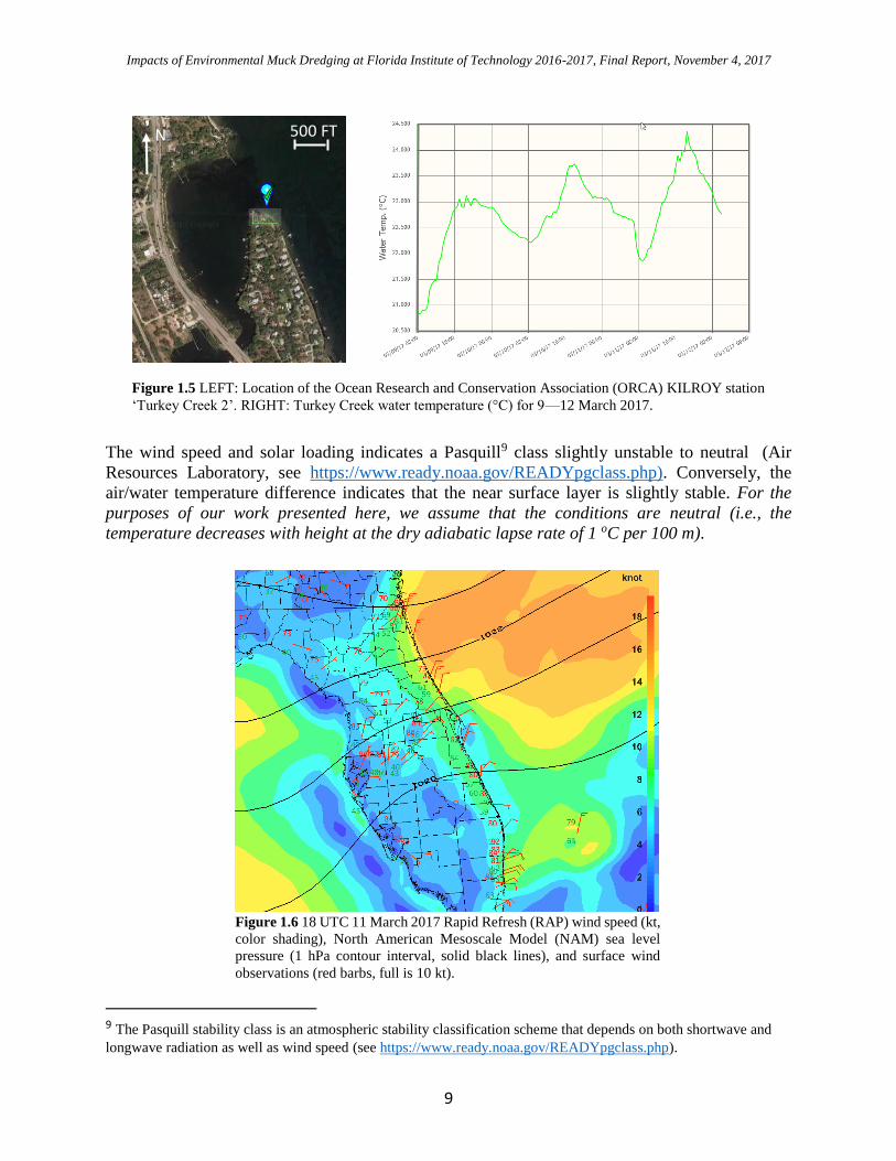
1.2 Synoptic Pattern and Water Temperatures: 11 March 2017
A surface high was situated to the north of the area resulting in a meridional (north/south) pressure
gradient over central and north Florida (Fig. 1.6). The gradient and associated on-shore
(northeasterly) flow increased to the north with the strongest surface winds roughly from Daytona
to Jacksonville. As shown in Figures 1.13 and 1.16, the 11 m flow was not steady through the 4 h
window but instead increased on the order of 4 kt (from 7 kt to 11 kt) with a lidar average of 8.4
kt (Table 1.3). Air temperatures were near 80 F (27 °C) while water temperatures at the ORCA
Turkey Creek Kilroy station were 22-23 °C (Fig. 1.5). There was full sun (with March insolation).
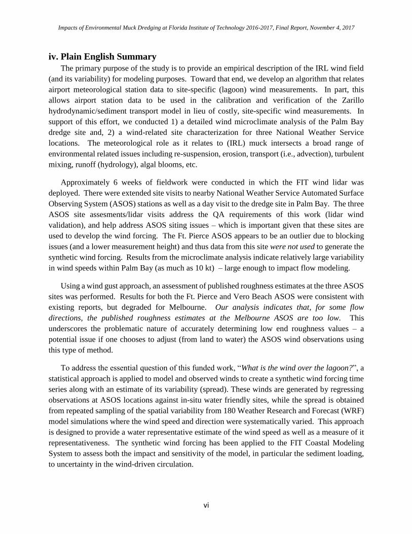
Figure 1.3 Palm Bay fetch analysis (m) versus wind direction (degrees) based on
the lidar location on 11 March 2017 (28.03659; -80.58199). See text for details.
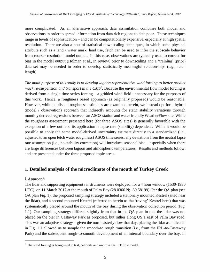
Figure 1.4 Fetch analysis for the Palm Bay lidar deployment on 11 March 2017.
Fetch rays originate from the lidar location in increments of 10°, ranging
clockwise from 10°-to-140° (northeast-to-southeast).
500 FT
N N
2000 FT
Impacts of Environmental Muck Dredging at Florida Institute of Technology 2016-2017, Final Report, November 4, 2017
9
The wind speed and solar loading indicates a Pasquill9 class slightly unstable to neutral (Air
Resources Laboratory, see https://www.ready.noaa.gov/READYpgclass.php). Conversely, the
air/water temperature difference indicates that the near surface layer is slightly stable. For the
purposes of our work presented here, we assume that the conditions are neutral (i.e., the
temperature decreases with height at the dry adiabatic lapse rate of 1 oC per 100 m).
9 The Pasquill stability class is an atmospheric stability classification scheme that depends on both shortwave and
longwave radiation as well as wind speed (see https://www.ready.noaa.gov/READYpgclass.php).
Figure 1.5 LEFT: Location of the Ocean Research and Conservation Association (ORCA) KILROY station
‘Turkey Creek 2’. RIGHT: Turkey Creek water temperature (°C) for 9—12 March 2017.
Figure 1.6 18 UTC 11 March 2017 Rapid Refresh (RAP) wind speed (kt,
color shading), North American Mesoscale Model (NAM) sea level
pressure (1 hPa contour interval, solid black lines), and surface wind
observations (red barbs, full is 10 kt).
N 500 FT

Impacts of Environmental Muck Dredging at Florida Institute of Technology 2016-2017, Final Report, November 4, 2017
10
1.3 Comparison of FIT lidar, Kestrel, and Remote ASOS
Because the Kestrel wind speeds were measured at a height of 2.59 m, a standard upward
adjustment to 11 m (i.e., assuming a neutral lapse rate atmosphere and homogeneous / flat terrain)
is applied:
0
059.211
59.2ln
11ln)(
z
zzUzU (2)
U(z11) and U(z2.59) are the wind speeds at 11 m and 2.59 m respectively, and z0 is the surface
roughness (taken here to be open / calm water surface, 0.0001). This results in approximately a 1
kt (0.2 kt) increase in the mean wind speed (standard deviation) as indicated in Table 1.3. Despite
the correction, the mean Kestrel wind speeds were slightly below (by about 0.8 kt), but within the
variability (i.e., < 1 ) of those observed by the lidar a few feet away (see Fig. 1.13). The remote
KMLB and KVRB ASOS stations observe higher wind speeds compared to the lidar. The ASOS
locations at most (but not all) airports, tend to be highly exposed (i.e., relatively low roughness).
To examine this in more detail, we provide z0 estimates from WeatherFlow (refrerred to as WF
hereafter) in Table 1.2. Indeed, this appears to be the case for KMLB and KVRB whose directional
roughness ranges from [0.0067, 0.0603] and [0.0081, 0.1176] with averages of 0.026 and 0.046
respectively. However, KFPR has some significant ‘blockage’, particularly in its northern sectors
due to forest (see Fig. 1.8) with directional roughness values ranging from [0.0044, 0.6572] and
an overall average of 0.2 – approximately an order of magnitude higher than KMLB and KVRB.
The wind direction for the three ASOS sites (Table 1.1) compares quite well – with the average
direction within 4° (see Table 1.3). The lidar however (which is located at the mouth of Palm Bay,
Fig. 1.1), observes a more northerly component and its average direction (24°) differs from the
three ASOS by 10-15°.
Table 1.1 ASOS station locations, ID, and name.
Station ID Location Name LAT LON
KMLB Melbourne International Airport 28.09973 -80.63560
KVRB Vero Beach Municipal Airport 27.65556 -80.41806
KFPR Fort Pierce 27.49806 -80.37667

Impacts of Environmental Muck Dredging at Florida Institute of Technology 2016-2017, Final Report, November 4, 2017
11
Table 1.2 WeatherFlow directional roughness estimates (m) for three ASOS locations Vero Beach (KVRB), Ft. Pierce
(KFPR) and Melbourne (KMLB. The direction (DIR, degrees) represents the bin center with width 22.5° (i.e., +/-
11.25°).
DIR KVRB KFPR KMLB
0.00 0.0559 0.5302 0.0103
22.50 0.1176 0.7647 0.0113
45.00 0.0438 0.6572 0.0067
67.50 0.0376 0.1166 0.0082
90.00 0.0428 0.0361 0.0088
112.50 0.0169 0.0049 0.0133
135.00 0.0081 0.0044 0.0317
157.50 0.0254 0.0459 0.0313
180.00 0.0451 0.1498 0.0628
202.50 0.0628 0.1508 0.0431
225.00 0.0564 0.1121 0.0414
247.50 0.0299 0.1096 0.0603
270.00 0.0229 0.0658 0.0212
292.50 0.0431 0.0756 0.0168
315.00 0.0922 0.1191 0.0214
337.50 0.0349 0.2533 0.0228
AVG 0.0460 0.1998 0.0257
Figure 1.7 Directional roughness (m) estimates for three National Weather Service
ASOS (KFPR, KMLB, and KVRB). Data provided by WeatherFlow.
0.001
0.01
0.1
1
0 60 120 180 240 300 360
rou
ghn
ess
len
gth
(m)
wind direction (degrees)
KFPR
KMLB
KVRB

Impacts of Environmental Muck Dredging at Florida Institute of Technology 2016-2017, Final Report, November 4, 2017
12
Table 1.3 Palm Bay wind speed statistics for 11 March 2017 (1528 UTC – 1937 UTC). The parentheses indicate that
the Kestrel winds have been adjusted (from 2.59 m) to the lidar range gate height of 11 m. The KFPR wind speed is
measured at 8 m and has been adjusted up to the WMO standard of 10 m so that it is consistent with KMLB and
KVRB.
mean speed
(kt)
std. deviation
(kt)
mean dir.
(deg)
std. deviation
(deg)
LIDAR 8.40 1.93 24.0 11.9
KESTREL (STATIONARY) 6.65 (7.60) 1.51 (1.73) NA NA
KMLB 10.2 1.71 40.6 11.5
KVRB 9.7 1.18 37.8 13.9
KFPR 7.65 (8.26) 1.18 (1.26) 44.6 17.3
1.4 Roving versus Stationary Kestrel
As previously mentioned, 6 sites (Fig. 1.1) were sampled for 20 minutes each, through the course
of the afternoon. In the presence of varying (non-stationary) wind speeds, the differences between
the roving and stationary Kestrels provide a means by which the winds can be compared
throughout the sampling period. With the exception of the pier (location 6), differences are
relatively small (< 1 kt). Given the northeast flow, it is not surprising that the roving Kestrel tended
observe lower wind speeds at sites 1, 2 , 4, and 5. However, site 3, located immediately to the
south of the lidar along the west shore of Palm Bay, appears to be slightly more fetch favorable
(hence the positive difference, i.e. roving greater than the stationary). While the variation is subtle
around the mouth of the bay, the pier had wind speeds that were on the order of 4 kt higher than at
the lidar. The exposed pier winds (adjusted to 10 m) are also higher than observed at the three
ASOS locations (Fig. 1.13) – although the wind speeds at KMLB (the smoothest of the three sites)
are close.
Figure 1.8 View looking north from the Treasure Coast
International Airport at the ASOS station site KFPR.

Impacts of Environmental Muck Dredging at Florida Institute of Technology 2016-2017, Final Report, November 4, 2017
13
Table 1.4 Wind speed statistics for 11 March 2017 (1528 UTC – 1937 UTC). The average differences (AVG DIF)
are calculated by subtracting the stationary Kestrel from the roving one.
SITE TIME
(UTC)
AVG SPEED
(kt)
AVG DIFF
(kt)
STDEV
(kt)
1 16.139 5.38 -0.675 1.99
2 16.714 5.90 -0.662 1.18
3 17.381 8.11 0.257 1.29
4 17.989 7.69 -0.025 1.19
5 18.547 6.47 -0.923 2.16
6 19.264 13.82 3.932 2.12
1.5 Vertical Profiles: Structure and Evolution of the Surface Layer
Although the lidar measures wind speed for as many as 10 range gates from 10 m up to 300 m, for
our sampling strategy on 11 March 2017 we capped the sampling at 200 m and concentrated on
resolving the near surface winds. with majority of our sampling below 50 m (our range gates were
set at 10, 14, 19, 24, 29, 38, 59, 99, and 199 m)10.
All of the 10 min lidar wind profiles are shown as well as three half hour averages during the early
(15.2—15.5 UTC), middle (17.2—17.5 UTC), and latter (18.7—19.0 UTC) part of the sampling
(Fig. 1.9). The cooler (warmer) colors represent the early (later) profiles. Wind speeds are
relatively uniform above 50 m (Ekman layer) while the surface layer is evident below that. As the
wind speeds increase, the profiles gradually migrate from left-to-right between 15—19 UTC. The
impact of the surface is also evident in the wind direction profile with the winds initially becoming
more northerly with height from the surface up to 50 m. Above this, the Ekman layer is evident
with winds becoming more geostrophic with height – gradually turning clockwise on the order of
10° between 50 and 200 m. The cross isobaric flow of the surface layer is apparent in Figure 1.6.
The increasing wind speed and decreasing deflection with height results in the Ekman wind spiral
through the lowest kilometer or so of the atmosphere (friction layer). This layer is undercut by the
surface layer where the log law better represents the winds near the ground. The depth of the
surface layer depends on stability, is maintained by vertical momentum transfer from turbulent
eddies and does not directly depend on the Coriolis or pressure gradient forces.
10 One must add 1 m to the range gates to account for the lidar measurement height.

Impacts of Environmental Muck Dredging at Florida Institute of Technology 2016-2017, Final Report, November 4, 2017
14
Although the log-law assumes that the wind direction does not change with height – this is not the
case here. However, some wind direction variation near the surface would be expected given the
heterogeneous land / water mix a few hundred meters upstream from the lidar.
Assuming neutral stability and homogeneous / flat terrain, the wind speed should increase linearly
with the the logarithm of height (the so-called log law). However, if the flow is disrupted by a
change in roughness – a new equilibrium forms. Because the lower atmosphere is responding to
surface elements, an internal boundary layer forms beneath the established upstream profile. In
Figure 1.9 LEFT: Lidar 10 min average wind speed profiles from 15 to 20 UTC 11 March 2017. The warmer
(cooler) colors are later (earlier) in the time window. RIGHT: 30 min average profiles for an early (15.2-15.5
UTC), middle (17.2-17.5 UTC), and later (18.7-19.0 UTC) time window of the observation period.
Figure 1.10 Same as in Fig. 1.9, but for wind direction (deg).
Impacts of Environmental Muck Dredging at Florida Institute of Technology 2016-2017, Final Report, November 4, 2017
15
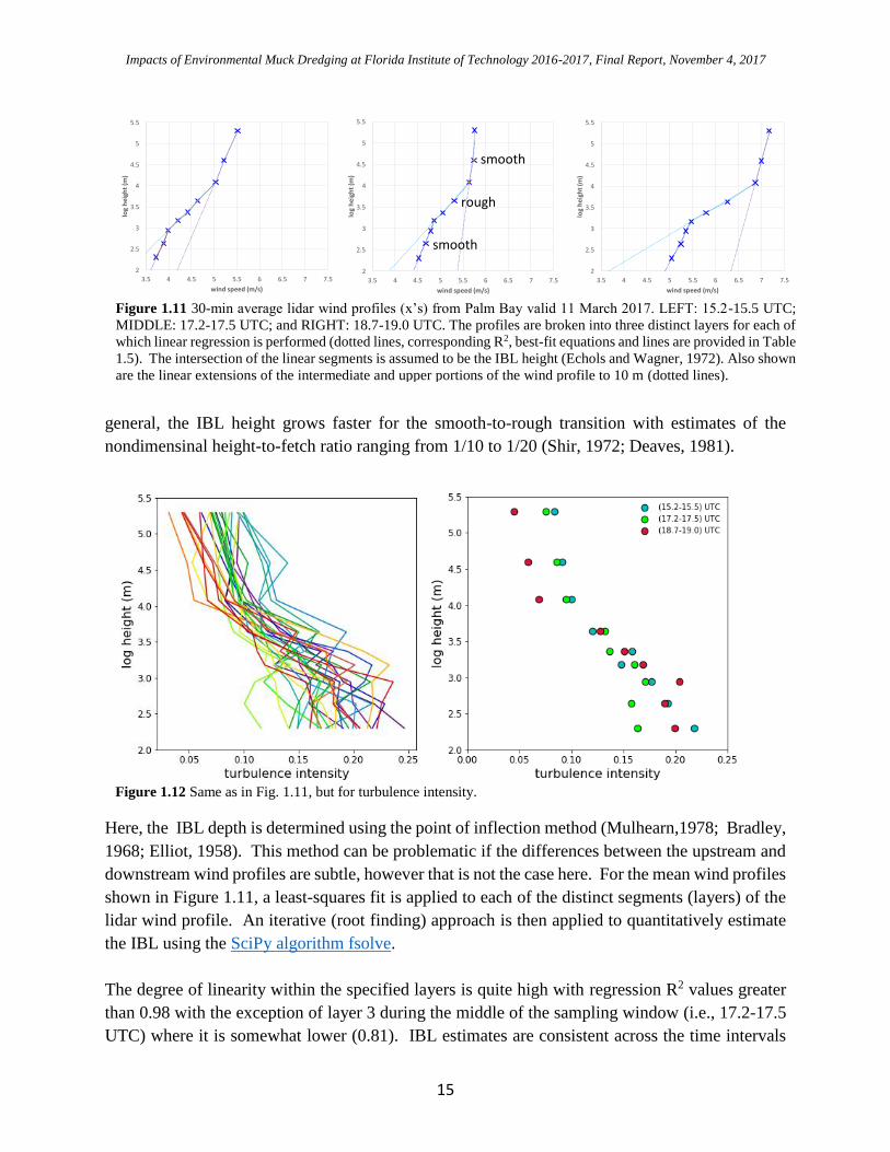
general, the IBL height grows faster for the smooth-to-rough transition with estimates of the
nondimensinal height-to-fetch ratio ranging from 1/10 to 1/20 (Shir, 1972; Deaves, 1981).
Here, the IBL depth is determined using the point of inflection method (Mulhearn,1978; Bradley,
1968; Elliot, 1958). This method can be problematic if the differences between the upstream and
downstream wind profiles are subtle, however that is not the case here. For the mean wind profiles
shown in Figure 1.11, a least-squares fit is applied to each of the distinct segments (layers) of the
lidar wind profile. An iterative (root finding) approach is then applied to quantitatively estimate
the IBL using the SciPy algorithm fsolve.
The degree of linearity within the specified layers is quite high with regression R2 values greater
than 0.98 with the exception of layer 3 during the middle of the sampling window (i.e., 17.2-17.5
UTC) where it is somewhat lower (0.81). IBL estimates are consistent across the time intervals
Figure 1.11 30-min average lidar wind profiles (x’s) from Palm Bay valid 11 March 2017. LEFT: 15.2-15.5 UTC;
MIDDLE: 17.2-17.5 UTC; and RIGHT: 18.7-19.0 UTC. The profiles are broken into three distinct layers for each of
which linear regression is performed (dotted lines, corresponding R2, best-fit equations and lines are provided in Table
1.5). The intersection of the linear segments is assumed to be the IBL height (Echols and Wagner, 1972). Also shown
are the linear extensions of the intermediate and upper portions of the wind profile to 10 m (dotted lines).
2
2.5
3
3.5
4
4.5
5
5.5
3.5 4 4.5 5 5.5 6 6.5 7 7.5
logheight(m
)
windspeed(m/s)
2
2.5
3
3.5
4
4.5
5
5.5
3.5 4 4.5 5 5.5 6 6.5 7 7.5
logheight(m
)
windspeed(m/s)
2
2.5
3
3.5
4
4.5
5
5.5
3.5 4 4.5 5 5.5 6 6.5 7 7.5
logheight(m
)
windspeed(m/s)
Figure 1.12 Same as in Fig. 1.11, but for turbulence intensity.
rough
smooth
smooth

Impacts of Environmental Muck Dredging at Florida Institute of Technology 2016-2017, Final Report, November 4, 2017
16
with a small increase from the first-to-second 30 min period. The lowest (19.2-23.7 m) kink in the
wind profile represents the top of the IBL that has formed downwind of Castaway Point Park
(rough-to-smooth transition). The second layer, which has enhanced shear compared to the
surface, is the upstream (residual) IBL generated as the flow crosses from the IRL to land along
the northeast portion of Palm Bay (smooth-to-rough transition). For an average wind direction of
20º (see Fig. 1.15), the fetch length (at the lidar) is approximately 350 m (Fig. 1.3) which yields a
height-to-fetch ratio of 1/18 for the Palm Bay IBL. The IBL growth is much steeper over land as
the second layer has an IBL height near 60 m. Assuming an approximate 120 m transit across
Castaway Park, this yields a height-to-fetch ratio on the order of 1/2.
Table 1.5 Least-squares coefficients based on three 30-min average lidar wind profiles on 11 March 2017 at Palm
Bay. Layer 1 represents the lower portion of the surface layer up to 25 m, layer 2 ranges from 20-to-60 m, and layer
3 extends from 60-to-200 m above ground level. The intercept is the natural log of the height, and the ratio of the
intercept-to-slope is related to the surface roughness (see Fig. 1.11).
slope intercept R2
15.2-15.5 UTC
Layer 1 2.3762 -6.5666 0.9834
Layer 2 1.0909 - 1.4169 0.9987
Layer 3 2.5026 - 8.4895 0.9973
17.2-17.5 UTC
Layer 1 2.517 - 9.0815 0.9907
Layer 2 1.1593 - 2.4783 0.9937
Layer 3 7.906 - 40.509 0.8142
18.7-19.0 UTC
Layer 1 2.0256 - 7.9252 0.9926
Layer 2 0.6441 - 0.362 0.9969
Layer 3 3.9143 - 22.799 1.0000
In addition to the wind profiles, we also show the lidar turbulence intensity TI (Eq. 1) as a function
of height (Figure 1.12). As expected, the TI peaks near the surface with values on the order of
0.20—0.25 and decrease with values on the order of 10-2 in the lower portion of the Ekman layer.
In general, TI is on the order of 0.10—0.15 in the near-neutral surface layer with larger values in
unstable and convective boundary layers (Arya, 2001). The 3 layers that comprise the Palm Bay
IBL, Castaway Park, and the residual IRL layer manifest in the TI – and are especially noticeable
in the average profiles with relatively distinct transitions between each. This is particularly
obvious during the later time window between the rough layer and residual IRL layer above it. A
number of the profiles peak just above the surface (at 25 m – the third lidar range gate). This
secondary maximum also appears in the mean profiles and is likely indicator of a convective
(unstable) surface layer.

Impacts of Environmental Muck Dredging at Florida Institute of Technology 2016-2017, Final Report, November 4, 2017
17
Table 1.6 Palm Bay IBL height (m) for three 30-min time intervals 11 March 2017. The IBL height, estimated via a
SciPy iterative root finding algorithm is the intersection of these two curves.
time
(UTC)
Palm Bay IBL
Height (m)
Castaway IBL
Height (m)
15.2-15.5 19.2 57.3
17.2-17.5 23.6 57.8
18.7-19.0 23.7 57.8
Figure 1.13 10 m wind speed (kt) 11 March 2017 at KMLB (blue line), KVRB (orange line), KFPR (gray line),
lidar (pink line), stationary Kestrel (light gray circles), and “roving” Kestrel at (see Fig. 1.1 for site locations):
site1 (red circles), site2 (green circles), site3 (purple circles), site4 (black circles), site5 (cyan circles), and site6
(orange circles). The Kestrel wind speeds were adjusted from 2.59 m to 10 m while KFPR were adjusted from 8 m
to 10 m (assuming neutral conditions). Also shown are the mean wind speeds at each site (+ signs with yellow
background).
0
2
4
6
8
10
12
14
16
18
20
15.0 16.0 17.0 18.0 19.0 20.0
win
d s
pe
ed
(kt
)
time (UTC)
KMLB
KVRB
KFPR
LIDAR (Palm Bay)
PB SITE1
PB SITE2
PB SITE3
PB SITE4
PB SITE5
PB SITE6
STN Kestrel
SITE AVG

Impacts of Environmental Muck Dredging at Florida Institute of Technology 2016-2017, Final Report, November 4, 2017
18
Figure 1.14 Same as in Fig. 1.13 but for Kestrel wind speed differences (roving – stationary) at the six
locations along Palm Bay on 11 March 2017. Vertical gray bars depict the site standard deviations (1
sigma).
-8.0
-6.0
-4.0
-2.0
0.0
2.0
4.0
6.0
8.0
10.0
15.5 16 16.5 17 17.5 18 18.5 19 19.5
win
d s
pe
ed
dif
ere
nce
(kt
)
time (UTC)
Figure 1.15 Lidar wind direction (z = 11 m) at 20 s intervals (degrees, filled green circles) and 10 min
average (blue circles/line) 11 March 2107 (Palm Bay). Values less than zero are from directions west of
due north (i.e., subtract 360°).

Impacts of Environmental Muck Dredging at Florida Institute of Technology 2016-2017, Final Report, November 4, 2017
19
1.6 Wind Direction and Fetch
Here we examine the impact of wind direction (and thus fetch) on the lidar observed flow. A
simple fetch-based model can be used to assess the micrometeorology of Palm Bay. Ideally, one
would perform very high resolution large-eddy simulations to resolve the IRL, its tributaries and
bays. However a parameterized approach is inexpensive, can be compared directly to model
output, and can be used to downscale coarse resolution model winds.
The impact that local roughness elements on the surface flow is assessed via the ratio of the 100
m to 11 m wind speeds (Fig. 1.16). As previously discussed, changes in this ratio generally reflect
the degree in which proximity surface obstructions influence the 11 m wind with values
approaching unity (> 1) for low (high) surface roughness.
In this case, the 100 m wind should be above the blending height (i.e., above the effects of local
surface elements). As Figure 1.16 indicates, U100 > U11, for the 10 min average wind speeds – the
10 m (100) average is 8.4 kt (10.95 kt). However, the difference between the two levels varies –
with some periods where they are within 1–2 kt of each other (i.e., between 16–17 UTC; 18 UTC).
The scatter about the 10 min curves indicates, as one would expect, more variability near the
surface. This will be discussed later in more detail.
To quantify the impact of the roughness transition upstream of the lidar (Castaway Point) the ratio
is first regressed against wind direction. Three slightly different least squares solutions are shown
Figure 1.16 Lidar wind speed (kt, approximate 20 s intervals) at 11 m and 100 m (open green and
black circles respectively) 11 March 2017. Also shown is the 10 min average at the two levels
(solid lines).

Impacts of Environmental Muck Dredging at Florida Institute of Technology 2016-2017, Final Report, November 4, 2017
20
for which the independent variable is the wind direction at 10 m (black x’s), 100 m (red crosses)
and an average over 0–100 m (blue open circles). The R2 values are marginally better using the
layer average wind directon, but the results are similar with decreasing ratios as the wind direction
changes from north-to-northeast.
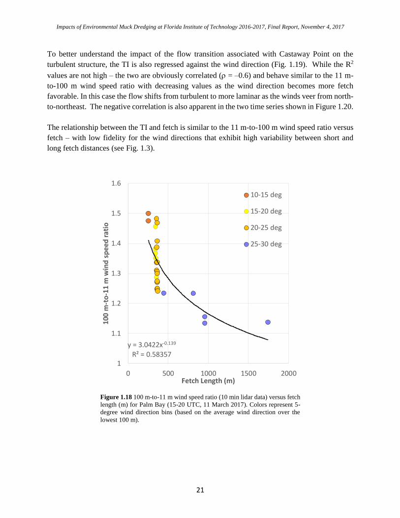
The decreasing ratio as the winds veer (i.e., turn clockwise) is obvious if the lidar relative fetch
(see section 1.1) is used instead of the wind direction (Fig. 1.18). In this case, the ratio approaches
1 (1.5) for the longer (shorter) fetch directions 25–30° (10-15°). There is a lack of fidelity at fetch
lengths on the order of 350 m for the intermediate directional bins (15–20°, and 20–25°). The
fetch assessment indicates a large jump (order of magnitude) near a wind direction of 30° (see Fig.
1.3). This not surpising given the considerable directional variability within these two bins (the
spread is on the order of +/– 25°, Fig. 1.15). The variabilty decreases for the wind directions with
longer fetch lengths. A power law fit relating the 100-to-11 m wind speed and fetch length is
provided on the figure. The fit provides a zero order model that can be used to map the 100 m lidar
wind speed to a high resolution grid of Palm Bay (a reasonable assumption if 100 m is above
blending height) using the regression equation and an estimate of the fetch length on the defined
grid.
Figure 1.17 100 m-to-11 m wind speed ratio (10 min lidar data) versus wind
direction for Palm Bay (15-20 UTC, 11 March 2017). Colors represent 11 m
(black X’s), 100 m (red +’s), and average 0-to-100 m (open blue circles) wind
directions respectively.
y = -0.0158x + 1.7032R² = 0.5141
y = -0.0182x + 1.7114R² = 0.56296
y = -0.018x + 1.7107R² = 0.6103
1
1.1
1.2
1.3
1.4
1.5
1.6
0 10 20 30 40
10
0 m
-to
-11
m w
ind
sp
eed
rat
io
wind direction (deg)
Impacts of Environmental Muck Dredging at Florida Institute of Technology 2016-2017, Final Report, November 4, 2017
21
To better understand the impact of the flow transition associated with Castaway Point on the
turbulent structure, the TI is also regressed against the wind direction (Fig. 1.19). While the R2
values are not high – the two are obviously correlated ( = –0.6) and behave similar to the 11 m-
to-100 m wind speed ratio with decreasing values as the wind direction becomes more fetch
favorable. In this case the flow shifts from turbulent to more laminar as the winds veer from north-
to-northeast. The negative correlation is also apparent in the two time series shown in Figure 1.20.
The relationship between the TI and fetch is similar to the 11 m-to-100 m wind speed ratio versus
fetch – with low fidelity for the wind directions that exhibit high variability between short and
long fetch distances (see Fig. 1.3).
Figure 1.18 100 m-to-11 m wind speed ratio (10 min lidar data) versus fetch
length (m) for Palm Bay (15-20 UTC, 11 March 2017). Colors represent 5-
degree wind direction bins (based on the average wind direction over the
lowest 100 m).
y = 3.0422x-0.139
R² = 0.583571
1.1
1.2
1.3
1.4
1.5
1.6
0 500 1000 1500 2000
100
m-t
o-1
1 m
win
d s
pe
ed r
ati
o
Fetch Length (m)
10-15 deg
15-20 deg
20-25 deg
25-30 deg

Impacts of Environmental Muck Dredging at Florida Institute of Technology 2016-2017, Final Report, November 4, 2017
22
Figure 1.19 11 m turbulence intensity versus the average (over the lowest
three lidar levels) wind direction for the Palm Bay lidar data 15-19 UTC 11
March 2017.
Figure 1.20 11 m turbulence intensity (blue line) and wind direction (red line) versus time (UTC) for
the Palm Bay lidar data 15-19 UTC 11 March 2017. See text for details.

Impacts of Environmental Muck Dredging at Florida Institute of Technology 2016-2017, Final Report, November 4, 2017
23
2. ASOS Site Characterization
i. Approach
While the three site assesments/lidar visits were relatively short, ranging from 1-3 weeks
deployment they are useful per the QA plan requirements. Because a long time series is necessary
in order to provide a more thorough assessment of an individual site, we also provide composite
statistics for three years at each of the ASOS locations. This climatology is compared against
published roughness estimates. The composite statistics include wind roses, gustiness roses and
histograms. Similar to the TI and the 100 m-to-11 m wind speed ratio, the gustiness is a proxy for
surface roughness. Gustiness is defined here as
1max U
UG , (3)
where Umax and U are the peak measured and mean wind speed over a specified time interval. For
the lidar, the temporal averaging period is 10 min. A wind rose contains three distinct pieces of
information including: wind direction, frequency and speed. When constructed over long time
periods, wind roses provide a climatological assessment tool for a particular observation location.
However, they can also be used to generate climatological fetch maps over an estuary (Holman et
al., 2015). The wind roses that are presented here were composited using a three-year period (2014-
2016) and 1-minute data (the highest temporal resolution available). The data counts, presented
Figure 1.21 Turbulence intensity (10 min lidar data) versus fetch
length (m) for Palm Bay (15-20 UTC, 11 March 2017).

Impacts of Environmental Muck Dredging at Florida Institute of Technology 2016-2017, Final Report, November 4, 2017
24
in Table 2.1, are significant (over 1.5 million each) with only a 2-4% dropout. The reliability of
the ASOS data is paramount to providing a continuous (uninterrupted) time series of wind
forcing.
Comparison with other sites can be used to assess the representativeness of a particular observation
location. The latter is particularly useful for the purposes of this work because we developing an
alternative wind forcing time series for the environmental modeling component of the IRL EMD.
The site visit and triennial statistics are presented separately for each site below.
Table 2.1 Total number of observations used to generate the three ASOS wind roses: KVRB, KFPR, and KMLB.
ASOS STATION Total # Observations % Reported
KVRB 1,540,730 97.71
KFPR 1,539,848 97.66
KMLB 1,514,693 96.06
ii. Results and Discussion
2.1 Vero Beach (KVRB)
The lidar was located within 100 feet of the Vero Beach ASOS for a 2-week period (25 March –
6 April 2017). The minimum, maximum and average wind speeds during this period are provided
in Table 2.2. In order to reduce the number of spurious calm reports, the ASOS wind statistics
were compiled using the 1 min data rather than 5 min data11 (the METAR coding used to report
surface observations beginning July 1996, a calm wind is defined as a wind speed less than 3 kt
and is assigned a value of 0 knots). The 1 min data is actually a running 2-minute average wind
(direction and speed) comprised of 5 s samples.
The lidar-ASOS comparison (mean speed) for the period is quite good (within 0.5 kt) – a small
part of which can be explained by the 1 m difference in the observation heights.
The wind roses are also quite similar – with predominantly southeast flow during the period (note
the scales are slightly different with respect to the frequency radii, Fig. 2.1). The wind direction
varied between 90-180° for about half of the observation period with the strongest winds from the
southeast (120°). The wind speed exceeded 10 kt for a large portion of the southeast flow but was
lighter from the the west, southwest and east. At 100 m, the wind rose has a directional distribution
11 For more details regarding ASOS metadata see https://www.ncdc.noaa.gov/data-access/land-based-station-
data/land-based-datasets/automated-surface-observing-system-asos.

Impacts of Environmental Muck Dredging at Florida Institute of Technology 2016-2017, Final Report, November 4, 2017
25
Table 2.2 Vero Beach (KVRB) ASOS and lidar wind statistics (at 11 m and 100 m) for 25 March – 6 April 2017.
min speed
(kt)
max speed
(kt)
mean speed
(kt)
LIDAR (11 m) 1.30 23.16 8.67
LIDAR (100 m) 1.57 26.16 13.16
ASOS 0.0 25.0 8.21
that closely resembles the 11 m wind – but the winds are higher from all directions with peak
winds greater than 18 kt in most bins.
A scatter plot of the 100 m versus 11 m lidar wind speeds is shown in Figure 2.2. The spread is
larger for lighter wind speeds. The reduced spread for higher wind speeds is, at least in part, due
to mechanical mixing (shear) which acts to reduce the vertical gradient. On occasion, the 11 m
wind exceeds the 100 m flow. This occurs for some light northwest flow and for southeast flow
at higher wind speeds (6-10 m/s). As discussed earlier, the closer the ratio is to one, the smoother
the surface (i.e., smaller roughness
In general, the southeast flow (cyan filled circles) lies close to the one-to-one line while the
southwest flow (yellow-green filled circles) exhibit large spread, especially for wind speeds less
than 6 m/s. The ratio peaks for light winds with values as large as 8-to-1.
The gustiness is shown as both a histogram and as a wind rose in Figure 2.3. These statistics were
derived from using three years of 10 m wind data from 2014-2016. The largest (smallest) gust
factors occur for northerly (west-to-northwest) flow. For the most part, gustiness compares
favorably to the directional roughness variation (see Fig. 2.4). However, the published data (WF,
Figure 2.1 Wind roses (speed kt, color) for the 25 March – 6 April 2017 sampling period at KVRB. LEFT: KVRB
ASOS; MIDDLE: FIT lidar (at 11 m, 10 min data); RIGHT: FIT lidar (at 100 m, 10 min data). Wind direction is
indicated along the perimeter. The wind rose radii indicate the % time the wind blows from that particular direction
during the time window.

Impacts of Environmental Muck Dredging at Florida Institute of Technology 2016-2017, Final Report, November 4, 2017
26
Fig. 1.7) indicate a minimum for southeast flow (from 135°) with a second, less pronounced,
minimum for westerly winds (from 270°). If we ignore the measurement chain, the gust factor can
be related to the roughness via
0
lnz
z
gcG
, (4)
where is the von Karman constant (typically set = 0.4), c is the dimensionless standard deviation
in neutral conditions, and g is the standardized gust (i.e., the difference between the maximum gust
and mean wind divided by the standard deviation). According to Eq. (4), plotting ln(z0) versus –
1/G should be approximately linear with slope equal to gc and an intercept of ln(z). Here we
interpolate the gustiness (10° bins) to the WF roughness directional resolution (22.5°). While most
of the points are in good agreement with the best-fit line, the R2 value is only 0.32 (Fig. 2.4). We
highlight four of the points as ‘outliers’ and include the directions for each. The most significant
discrepancy, i.e. flow from 135°, is the minimum z0 per WF, but only corresponds to a relative
minimum in gustiness (see histogram, Fig. 2.3). Conversely, flow from 315° has the lowest
gustiness but the reported z0 is relatively high for the station (see Table 1.2 or Fig. 1.7).
Figure 2.2 KVRB lidar 100 m-to-11 m wind speed ratios (25 March – 6 April 2017). LEFT: linear axes; RIGHT: log
axes. Filled colors indicate wind direction.

Impacts of Environmental Muck Dredging at Florida Institute of Technology 2016-2017, Final Report, November 4, 2017
27
The corresponding three-year wind rose indicates that easterly flow dominates this site with the
highest wind speeds from the southeast (Fig. 2.5). Although less frequent, west-to-northwest flow
also experience some higher wind speeds – both of which are consistent with the relative minima
in the gustiness/roughness for these directions. Despite having less frequent westerly flow, the
percentage of low wind speeds is greater than for easterly flow. Interestingly, southerly winds are
as infrequent as northerly at KVRB.
Figure 2.3 Three-year (2014-2016) gustiness G (Eq. 3) climatology for the KVRB ASOS as a function of wind
direction (degrees x 10). LEFT: histogram (bin width is 10°); RIGHT: Polar plot (rose) with magnitude given in color).
See text for details.
Figure 2.4 The ln(z0) versus the negative reciprocal of the gust factor for KVRB. The gust factors
were estimated using a 3-year time series of 10 m winds (2014-2016). Each of the filled circles
represents a particular wind direction (16 bins, 22.5° bin width). The corresponding directional
roughness estimates z0 were obtained from the WeatherFlow. Four ‘outliers’ are identified by the
embedded red circle and annotated with the wind direction.
wind direction (deg. x 10)
G

Impacts of Environmental Muck Dredging at Florida Institute of Technology 2016-2017, Final Report, November 4, 2017
28
2.2 Fort Pierce (KFPR)
The lidar spent three weeks at the Fort Pierce airport alongside (i.e., within 100 ft of) the KFPR
ASOS. The lidar and ASOS mean winds are within 1 kt of each other during the 8 to 30 April 2017
sampling period. Given that the wind sensor at the Fort Pierce ASOS is sited at 8 m instead of the
10 m, the 3 m difference in the instrument heights can explain some (if not all) of the observed
discrepancy for which the lidar is systematically higher. The 100 m winds are, on average, about
4.2 kt higher than the 10 m. Although the average (for all directions) WF roughness at KVRB is
an order of magnitude lower than KFPR (see Table 1.2), the ratio, 1.41, is lower than that at KVRB
(1.52). However, this is consistent with the observed east-to-southeast flow where the directional
z0’s are one-to-two orders of magnitude lower than for other directions (see Table 1.2 or Fig. 1.7).
Table 2.3 ASOS and lidar wind statistics for 8 April – 30 April 2017 (at Fort Pierce, KFPR).
min speed
(kt)
max speed
(kt)
mean speed
(kt)
LIDAR (11 m) 1.2 22.4 10.3
LIDAR (100 m) 1.5 27.4 14.5
ASOS 0.0 24.0 9.4
As at KVRB, the ASOS and lidar wind roses compare favorably (Fig. 2.6). The highest (10 m)
wind speeds during the April sampling were from the southeast. Approximately 14% of the flow
was from the east (90°) while southeast flow (130°) was present in 10-11% of the sampled winds.
The 100 m winds are similar to the 10 m – with largest percentage of the highest wind speeds (>
18 kt) in the 130° and 90° directional bins.
Figure 2.5 Three-year (2014-2016) wind rose for the KVRB ASOS.
The thick black circle is the 2% frequency radii.

Impacts of Environmental Muck Dredging at Florida Institute of Technology 2016-2017, Final Report, November 4, 2017
29
The same wind ratio (100-to-11 m) is shown for KFPR in Figure 2.7. The southeast and east flow
directions dominate the scatter plot (cyan and blue-filled circles). There is about a 3 m/s spread
between the two levels at low wind speeds, decreasing to about 1 m/s as the wind increase (i.e.,
greater than 10 m/s). The easterly flow exhibits slightly higher ratios (for wind speeds greater
than 4 m/s) compared to southeast flow. This can be seen as the string of unobstructed darker blue
circles that are visible along the upper edge of the southeast flow (cyan circles). This is consistent
with the WF roughness, which is a minimum for southeast flow. The ratio increases for southeast
flow at lower surface wind speeds (less than 4 m/s) as can be seen in the log plot (right panel Fig.
2.7). This may, in part, be stability related (decoupling).
Figure 2.6 Wind roses (speed kt, color) for the 8 April – 30 April 2017 sampling period at KFPR. LEFT: KFPR
ASOS; MIDDLE: FIT lidar (at 11 m, 10 min data); RIGHT: FIT lidar (at 100 m, 10 min data). Wind direction is
indicated along the perimeter. The wind rose radii indicate the % time the wind blows from that particular direction
during the time window.
Figure 2.7 KFPR lidar 100 m-to-11 m wind speed ratios (8 April – 30 April 2017). LEFT: linear axes; RIGHT: log
axes. Filled colors indicate wind direction. See text for description of red line in the left panel.

Impacts of Environmental Muck Dredging at Florida Institute of Technology 2016-2017, Final Report, November 4, 2017
30
Although less frequently observed during the sampling, northwest flow is evident with high scatter
(at 100 m) at the low wind speeds (less than 4 m/s). Some of these ratios are quite large – especially
for low wind speeds (7-to-1). As discussed, this flow direction is blocked by forest on the north
side of the airport and is consistent with the published (WF) z0 which ranges between 0.50—0.75
m (see Figs. 1.7 and 1.8). Given the northerly flow (cooler surface conditions), it is possible that
some of the scatter is also related to nocturnal surface inversions.
Some of the higher wind speeds for the southwest flow can also be seen to the upper right in both
figures. These ratios are distinctly higher than the southeast flow ratios – but are comparable to
those of the sampled easterly flow. This can be seen in Fig. 2.7 as the southwest flow (orange-
filled circles) has a similar slope that appears to be an extension of the easterly flow to higher wind
speeds (annotated red line). Obviously, a longer sampling interval would clearly be beneficial in
order to better populate the upper end of the 100 m wind speeds that were not observed for easterly
flow. Nonetheless, the lidar observations are consistent with the WF roughness estimates reported
herein (i.e., ENE and SW flow have similar z0’s).
The gustiness (Eq. 4) histogram and its corresponding wind rose for KFPR is shown in Figure 2.8.
The gustiness is relatively low for both southeast and westerly flow, and largest for northeasterly
flow. This produces an ellipse-like pattern (with major axis oriented along a northeast-southwest
direction) in the gustiness rose. The gustiness climatology is supported by the limited lidar
observations which exhibit lower wind speed ratios (smoother surface) for both the east-to-
northeast flow and southwesterly flow directions and high ratios for northerly flow associated with
trees along the northern perimeter of the Ft. Pierce airport (see previous discussion).
Figure 2.8 Three-year gustiness G (Eq. 3) climatology for the KFPR ASOS as a function of wind direction. LEFT:
histogram (bin width is 10°); RIGHT: Polar plot (rose) with magnitude given in color). See text for details.
wind direction (deg. x 10)
G

Impacts of Environmental Muck Dredging at Florida Institute of Technology 2016-2017, Final Report, November 4, 2017
31
For most wind directions, the gustiness estimates are in good
agreement with the WF roughness estimates with an R2 value of
0.78 (Fig. 2.9). Three directions that might be considered as
‘outliers’ are discussed briefly here. Despite the presence of a
glide slope to the west of the ASOS anemometer (Fig. 2.10), the
gustiness is low and comparable to the southeast flow direction.
This is not the case for the WF roughness estimates which are
low only for southeast flow, i.e., there is no second minimum for
westerly flow (Fig. 1.7). The z0’s reported (approximately
0.0045) for the 112.5° and 135.0° flow directions are the lowest
of the 16 cardinal directions in the WF data – two orders of
magnitude below that of the northeast flow direction. These z0
values appear to be on the low end compared to typical airport
values (or level grass plains) which generally range from 0.005
(cut grass at 3 cm) to 0.05 (airport runways). A roughness value
in this log interval of 10-2 m (midrange) would place the two
points close to the best-fit line shown in Figure 2.9.
The KFPR climatological wind rose also has a prevalence of east-to-southeast flow and a
secondary peak for northwest flow. However, of the three ASOS sites, KFPR appears to be an
outlier. In general, the peak wind speeds for most directions are lower at KFPR and occur less
frequently. In addition to being weaker (due to the blockage), northerly flow is also observed
slightly less often at KFPR.
Figure 2.10 View looking west
from KFPR. The ultrasonic (glide
slope) anemometer is foreground
(background).
Figure 2.9 The ln(z0) versus the
negative reciprocal of the gust factor
for KFPR. The gust factors were
estimated using a 3-year time series
of 10 m winds (2014-2016). Each of
the filled circles represents a
particular wind direction (16 bins,
22.5° bin width). The corresponding
directional roughness estimates z0
were obtained from the
WeatherFlow. Four ‘outliers’ are
identified by the embedded red circle
and annotated with the wind
direction.

Impacts of Environmental Muck Dredging at Florida Institute of Technology 2016-2017, Final Report, November 4, 2017
32
Even the southerly and southwesterly flow appears to be somewhat muted (i.e., less frequent)
compared to KVRB and KMLB. The majority of high winds are associated with southeast flow
(110°-140°), which is consistent with the relative minima in the gustiness and roughness for these
directions.
2.3 Melbourne (KMLB)
Unfortunately, the lidar was not co-located with the KMLB
ASOS during the sampling (21—27 January 2017), as it
was postioned south and west near the FIT aviation
building. Nonetheless, the lidar data are useful despite the
blockage (due to the FIT aviation facility) as they do
provide a means by which we can evaluate the blending
height. However, we do not provide a direct statistical
comparison with the ASOS for this site.
The obstruction is apparent in Figure 2.13 as the strong 10
m flow from the west in the ASOS observations is missing
from the lidar wind rose. In contrast, the southwest flow is
well resolved (in terms of frequency) by the lidar – however
the proportion of the higher wind speeds is reduced at the
lidar. This is most likely due to the land cover (forest, see
Fig. 2.12) along the southwest border of the airport (KMLB
is displaced northeast of the lidar). There is westerly flow
Figure 2.11 Three-year (2014-2016) wind rose for the KFPR ASOS. The thick black
circle is the 2% frequency radii.
Figure 2.12 View looking southwest of
the FIT lidar at the Melbourne
International Airport.

Impacts of Environmental Muck Dredging at Florida Institute of Technology 2016-2017, Final Report, November 4, 2017
33
present in the 100 m wind rose – with similar frequency (about 11%) to that observed at KMLB
(note the radii differ slightly). Applying the usual assumptions, the 100 m wind can be brought
down to 10 m using the ASOS directional roughness – and then compared. Other (lower) lidar
range gates could also be compared in the same fashion – an indirect way to estimate the blending
height. The 100 m lidar winds are subtantially higher than the 10 m ASOS and 11 m lidar.
The 100 m-to-11m scatter is also consistent with the flow blockage to the west (i.e., between about
260° and 290°, blue green to light orange-filled circles). The log plot indicates that the largest of
ratios are comprised of flow (green and orange filled circles respectively). The west-to-northwest
flow (300°, dark orange-filled circles) is relatively unobstructed with low ratios. Southwest flow
(blue circles) exhibits both large and small ratios at low wind speeds – and is most likely related
to stability driven decoupling of the surface wind from the 100 m flow (stratifying the data by time
of day would help determine whether this was the case or not).
Of the three sites, KMLB is the most uniform with respect to directional roughness with only small
variations in gustiness (Fig. 2.15). The gustiness wind rose is quite smooth from 300° (northwest)
to 110° (southeast flow) with the lowest values for west-to-northwest flow (from about 270° to
300°).
Figure 2.13 Wind roses (speed kt, color) for the the 21 January – 27 January 2017 sampling period at KMLB.
LEFT: KMLB ASOS; MIDDLE: FIT lidar (at 11 m, 10 min data); RIGHT: FIT lidar (at 100 m, 10 min data).
Wind direction is indicated along the perimeter. The wind rose radii indicate the % time the wind blows from that
particular direction during the time window.

Impacts of Environmental Muck Dredging at Florida Institute of Technology 2016-2017, Final Report, November 4, 2017
34
The dynamic range is low, especially compared to KFPR with most directions falling between
0.20 and 0.25. The lack of fidelity is responsible for the large scatter in the gustiness versus z0
regression. As a result, we do not present an outlier analysis for KMLB. In lieu of the published
roughness assessment, we provide a full regression of all three sites combined. The R2 is relatively
high at 0.64 (0.8 correlation), and the cluster of low z0’s (all of one of which are from KMLB, 5
blue and 1 green filled circle) stand out. Our gustiness analysis indicates that the WF roughness
estimates from these directions are likely too low.
Figure 2.14 KMLB lidar 100 m-to-11 m wind speed ratios (21 January – 27 January 2017). Filled colors indicate
wind direction.
Figure 2.15 Three-year gustiness G (Eq. 3) climatology for the KMLB ASOS as a function of wind direction.
LEFT: histogram (bin width is 10°); RIGHT: Polar plot (rose) with magnitude given in color). See text for details.
wind direction (deg. x 10)
G

Impacts of Environmental Muck Dredging at Florida Institute of Technology 2016-2017, Final Report, November 4, 2017
35
The KMLB climatological wind rose is quite similar to that of KVRB – with no blockage issues
and high frequency for east-southeast flow and secondary peak for northwest flow. Relatively
small differences from KVRB include easterly flow, which has a larger proportion of higher wind
speeds at KMLB (compare the highlighted 2% radii). Northeast flow (30º) is also a bit stronger at
KMLB – this is consistent with the WF roughness differences between the sites which are largest
for north-northeast flow (compare orange and gray lines in Fig. 1.7).
Figure 2.16 LEFT: The ln(z0) versus the negative reciprocal of the gust factor for KMLB. The gust factors were
estimated using a 3-year time series of 10 m winds (2014-2016). Each of the filled circles represents a particular
wind direction (16 bins, 22.5° bin width). The corresponding directional roughness estimates z0 were obtained from
the WeatherFlow. Four ‘outliers’ are identified by the embedded red circle and annotated with the wind direction.
RIGHT: Full regression for all three sites: KVRB (yellow), KFPR (green), and KMLB (blue).
Figure 2.17. Three-year (2014-2016) wind rose for the KMLB ASOS. The thick black circle is the 2% frequency radii.
Also shown, for comparison are KFPR and KVRB (2014-2016). The bold circle depicts the 2% occurrence threshold.

Impacts of Environmental Muck Dredging at Florida Institute of Technology 2016-2017, Final Report, November 4, 2017
36
3. Wind Forcing Time Series i. Approach
The basic idea is to combine proximity surface wind observations and Weather Research and
Forecast Model output to help construct a representative IRL water-friendly time series. Ideally
this source would be reliable (low amounts of missing data) and have good quality data (e.g.,
National Weather Service ASOS). The approach is summarized below for one of the
environmental flow domains.
Regress an ASOS station (e.g., KMLB) against a nearby water friendly observation (e.g.,
XRPT – Rocky Point) and add residual noise to generate an IRL representative wind
speed.
Identify WRF water points within the relevant CMS12 shape file (six total, Fig. 3.1) and
then remove “open ocean” water points (i.e., retain only IRL)
Mine the WRF output (180 simulations, 18 cardinal wind directions and 10 wind speed
bins) to generate wind speed histograms for each CMS domain (900 total).
Fit a Weibull distribution to each of the PDFs
Extend Weibull fit to higher wind speeds by regressing variance and scale against the
average WRF IRL wind speed within the EMS shape file.
Use the regressed KMLB wind speed (+ residual noise) to select the appropriate Weibull
distribution. Sample this distribution 1000 times to produce an uncertainty estimate.
12 Coastal Modeling System (Zarillo and Zarillo, 2011).
Figure 3.1 LEFT: Environmental model subdomains (Zarillo). RIGHT: The
Banana River subdomain (shape file, red line) and associated WRF IRL (red +’s)
and coastal ocean (green +’s) water points.
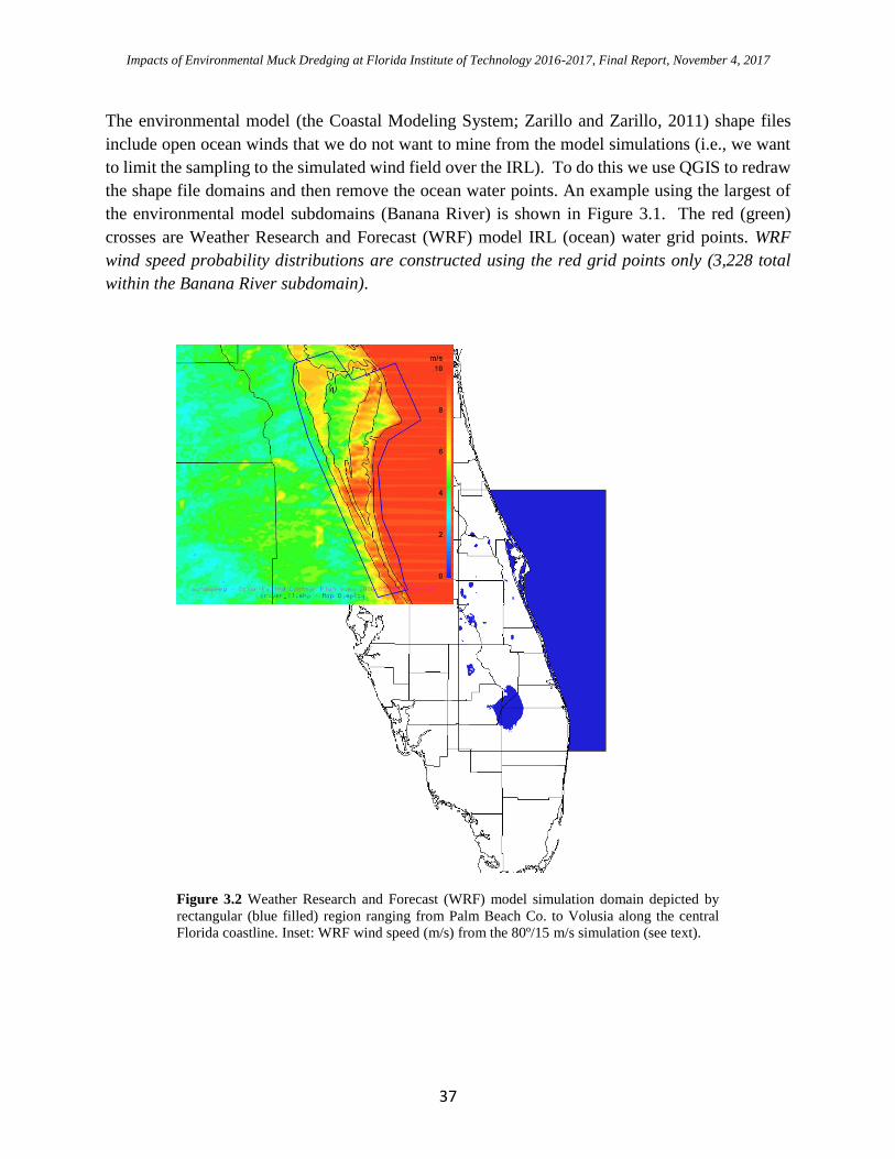
Impacts of Environmental Muck Dredging at Florida Institute of Technology 2016-2017, Final Report, November 4, 2017
37
The environmental model (the Coastal Modeling System; Zarillo and Zarillo, 2011) shape files
include open ocean winds that we do not want to mine from the model simulations (i.e., we want
to limit the sampling to the simulated wind field over the IRL). To do this we use QGIS to redraw
the shape file domains and then remove the ocean water points. An example using the largest of
the environmental model subdomains (Banana River) is shown in Figure 3.1. The red (green)
crosses are Weather Research and Forecast (WRF) model IRL (ocean) water grid points. WRF
wind speed probability distributions are constructed using the red grid points only (3,228 total
within the Banana River subdomain).
Figure 3.2 Weather Research and Forecast (WRF) model simulation domain depicted by
rectangular (blue filled) region ranging from Palm Beach Co. to Volusia along the central
Florida coastline. Inset: WRF wind speed (m/s) from the 80º/15 m/s simulation (see text).
Figure #. The Weather Research and Forecast Model (WRF) simulation domain (rectangle) and its land / water (blue) mask).

Impacts of Environmental Muck Dredging at Florida Institute of Technology 2016-2017, Final Report, November 4, 2017
38
ii. Results and Discussion
3.1 Weibull fit of the WRF Wind Speed Distributions
The Q-Q plot emphasizes the lack-of-fit at the distribution tails. These diagrams can be useful in
terms of discerning whether the theoretical curves are consistent with the sample quantities (here
– the WRF model winds), i.e., do they come from the same distributions. A “one-to-one” line is
typically included on the figure to indicate where the points should line up if the sample matches
the base distribution. The quantiles (or percentiles) are straight-forward and represent where a
particular value lies within the distribution (and thus data are first sorted from low-to-high values).
In the case for which the data are normally distributed about some mean value, then half the data
should be less than (or greater than) the mean. If the data are skewed towards the lower (higher)
tail the quantiles will increase more slowly (rapidly) when compared to the standard normal
distribution. The example shown in Figure 3.3 is comprised of IRL water points from a single
WRF simulation with a wind speed of 15 m/s and easterly wind direction of 80° (the wind speed
for this simulation is displayed as the inset in Fig. 3.2). The wind speed distribution appears to be
non-Gaussian with a left skewed peak (around 7 m/s) and somewhat broad right tail with peak
winds of 11 m/s. These equilibrium 10 m ‘IRL’ winds are lower (by about 30%) than the model
initialized flow (15 m/s). In this case, the easterly flow decelerates as it moves across the barrier
island (smooth-to-rough transition) and then reaccelerates as it crosses the IRL (rough-to-smooth
transition). The winds do not recover fully to the upstream open ocean magnitude (this is discussed
in more detail later in this section). In any case, the QQ-plot indicates that of the various Burr
distributions shown, the standard Burr appears to perform best. The maximum likelihood and
maximum goodness of fit estimation (MLE and MGE respectively) methods are shown – the latter
of which is applied using the Anderson-Darling left skewed distance metric (ADL)13. While the
left skew metric better fits the low end of the wind speed distribution, it performs poorly at the
upper end. Given our desire to reproduce ‘open water’ winds – we feel it is important to capture
the higher wind speeds in our parameterized distributions. Here, we opted for a Weibull fit
instead of those shown as its performance was more in line with our desired outcome
(retaining the higher wind speeds while simultaneously preserving the distribution shape). Weibull
is a standard for the wind industry.
In order to create probability density functions PDFs for “all” observed wind speeds14, we generate
scatter plots for two of the best-fit parameters from the histograms (variance and scale). In Figure
3.4, we show the resulting variance from a Weibull fit for each of the 180 simulations as a function
13 The statistics package has the option for eight different distance metrics for the MGE methodology. 14 While the WRF simulations capture the wind direction (i.e., there are 18 directional bins at 20° resolution), the 10
wind speed categories extend only to 15 m/s (and apply to open fetch only).

Impacts of Environmental Muck Dredging at Florida Institute of Technology 2016-2017, Final Report, November 4, 2017
39
of the average wind speed for the Banana River subdomain. Note that the Weibull variance 2 is
related to the distribution’s shape and scale parameter via
2
22 )1
1()2
1(
, (5)
where is the Gamma function. The variance (as a function of the mean ‘Banana
River’ WRF wind speed) is well-predicted by a power law relation. The WRF model indicates that
there is enhanced variability for increasing wind speed as well as larger spread that is associated
with the wind direction. In particular, the variance peaks for easterly flow – which is relevant given
the regional climatology favors this flow regime (e.g., see the 3-year wind roses for KVRB, KFPR,
and KMLB in Figs. 2.5, 2.11, and 2.17).
Figure 3.3 LEFT: Density histogram of WRF wind speeds from the 15 m/s @80° WRF simulation sampled
over the Banana River domain. Also shown are idealized fits for Burr, Burr-MLE (maximum likelihood
estimate) and Burr MGE-ADL (maximum goodness-of-fit estimation with the left tailed Anderson-Darling
distance metric) distributions from the R-statistics package fitdistrplus (Delignette-Muller and Dutang,
2015). RIGHT: Corresponding Q-Q plot of the empirical versus theoretical percentiles.
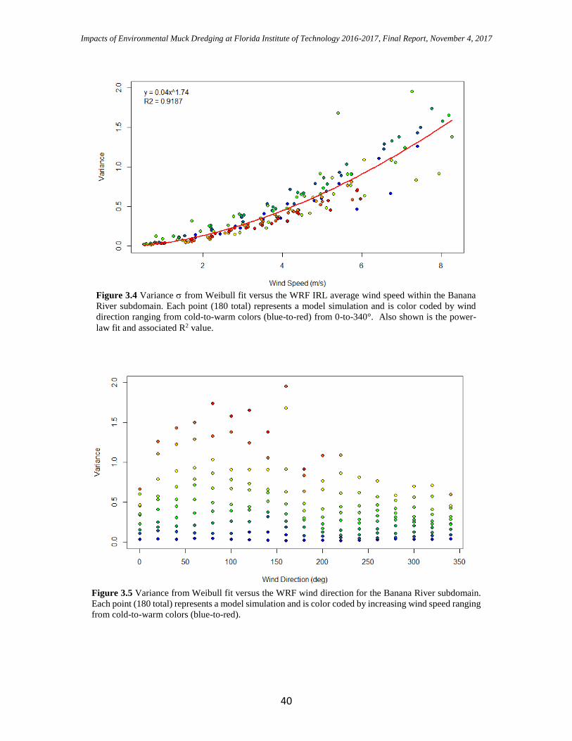
Impacts of Environmental Muck Dredging at Florida Institute of Technology 2016-2017, Final Report, November 4, 2017
40
Figure 3.4 Variance from Weibull fit versus the WRF IRL average wind speed within the Banana
River subdomain. Each point (180 total) represents a model simulation and is color coded by wind
direction ranging from cold-to-warm colors (blue-to-red) from 0-to-340°. Also shown is the power-
law fit and associated R2 value.
Figure 3.5 Variance from Weibull fit versus the WRF wind direction for the Banana River subdomain.
Each point (180 total) represents a model simulation and is color coded by increasing wind speed ranging
from cold-to-warm colors (blue-to-red).

Impacts of Environmental Muck Dredging at Florida Institute of Technology 2016-2017, Final Report, November 4, 2017
41
A second Weibull parameter is also shown in Figure 3.6. This parameter is highly linear with
respect to the average WRF wind speed (R2 = 0.9998, slope = 1.06). The third free-parameter
has far more scatter and is not shown here. However, from Eq. (5) it is clear that the three
parameters are not independent. Instead, given that is implicit in Eq. (5), we estimate it using the
variance and mean according to the following approximation (Rocha et al. 2012):
086.1
U
, (6)
where U is the mean wind speed (here it is the average WRF wind over the Banana River
subdomain). Once the three parameters are known, the Weibull PDF can be fully specified as
u
eu
uuf ),,( , (7)
where u is the wind speed and and are modeled using the variance model (polynomial fit),
linear model and Eq. (6). This approach allows us to extend the distributions to higher wind
speeds without additional (expensive) model simulations.
3.2 ASOS to ‘Water Friendly’ Regressions
Because the KMLB is a “land station”, we first regress the Melbourne ASOS to a nearby fetch
favorable WeatherFlow station Rocky Point (XRPT) – just south of Malabar, FL on the west shore
of the IRL (see Fig. 3.7). Although WeatherFlow generally places their sensors in fetch favorable
Figure 3.6 Weibull fit parameter (scale) from
each of the 180 WRF simulations. Color fill is the
same (i.e., direction dependent) as for the variance
in Fig. 3.4.

Impacts of Environmental Muck Dredging at Florida Institute of Technology 2016-2017, Final Report, November 4, 2017
42
locations, this is not always the case. To assess this issue, a 3.5-year climatology (histograms) for
six of their stations within the IRL is shown in Figure 3.8. We use Parrish Park (XPAR) as the
water friendly baseline as it is sited on a channel marker and thus surrounded by water in the
northern IRL (just north of the Max Brewer Parkway). The XRPT distribution is similar to that of
XPAR – especially the higher wind speed tail which is a good indicator of open fetch. Note that
this tail is absent in some of the other WeatherFlow locations shown including XVER (downtown
Vero Beach) and XDAI (Dairy Road in suburban Melbourne).
Figure 3.7 LEFT: Locations of the KMLB ASOS and WeatherFlow station XRPT. RIGHT: XRPT
versus KMLB wind speed (m/s) for November 2013. Shown are the one-to-one line (blue) and least
squares best-fit line (red), associated equation, and R2.
XRPT
KMLB
Figure 3.8 Wind speed (m/s) histograms (Jan 2013—May 2016) for six WeatherFlow
sites (LEFT top to bottom: XDAI, XAQU; RIGHT top to bottom: XPAR, XPRT, XVER
and XSTL) along the IRL. See Appendix D for individual histograms.
N
N

Impacts of Environmental Muck Dredging at Florida Institute of Technology 2016-2017, Final Report, November 4, 2017
43
In order to capture the intra-seasonal variability between sites, the regression is performed
monthly. The R2 values for each month are shown (2013-2015) in Figure 3.9. The regression was
performed for both all observations and for open fetch (at XRPT) only. It is interesting to note,
that the regression fit is better for ‘all’ observations during the warm months (April—October)
while the cool season (November—March) the regression favors the open fetch observations. In
general, the largest R2 differences occur during the warmest months (mid-summer). In part, the
differences are likely stability driven – with relatively cool (warm) water and corresponding higher
(lower) static stability in the spring (fall). In order to be consistent with our construction of the
three-year synthetic time series, we select the ‘all’ regression for each month.
As an example of the methodology, we apply the regression to November 2013 (Fig. 3.7, see
Appendices B and C for a list of all XRPT versus KMLB regression coefficients over 2013-2015).
Despite the relatively good correlation (R2 = 0.75 for November 2013), there is no reason to expect
(nor desire) the synthetic observations to fall directly on the best-fit line, i.e., the mapping of the
KMLB observation to the water friendly XRPT should have scatter. In order to account for this
variability, we add uncertainty by modeling the scatter as a linear function of the standard error of
the fit (i.e., mean absolute residual ), wind speed V , and a user specified multiplicative factor
that defines the standard deviation of the scatter, i.e.
V (8)
Assuming that represents a normal distribution (about the best-fit line), we sample the Gaussian
once for each observation mapping (i.e., for each 2-minute observation, once per hour). We
purposely avoid repeated sampling here as the most likely mapping will fall on the regression line.
Hence the synthetic wind Usyn field is given by
bUU KMLBsyn, (9)
where and b are the least-squares parameters (slope and intercept) from the monthly regression
and is the introduced variability. An example is shown for a value of equal to 0.05 in Figure
3.10 (November 2013). The dependent variable (y-axis) is the “regression + uncertainty” while
the predictor, KMLB observations comprise the x-axis. As the wind speed increases, the spread
follows as expected. Given that we are sampling from the same data (November 2013), despite
the introduced variability – the slope and intercept of the original fit are preserved (1.22 and 0.65
respectively, Fig. 3.10). As a secondary (QC/QA) check on the methodology, we also show the
XRPT observations regressed against the synthetic data. As expected, the slope is approximately
one-to-one (0.96) while the scatter is comparable to that of original regression shown in Fig. 3.7.
Finally, we show statistics (RMSE and bias) from ten different synthetic time series generated for
November 2013 (Table 3.1). As expected, the RMSE is reduced when compared to XRPT (versus

Impacts of Environmental Muck Dredging at Florida Institute of Technology 2016-2017, Final Report, November 4, 2017
44
KMLB) and the bias is near zero. Furthermore, the average bias between the synthetic time series
and KMLB (1.58) is nearly identical to that between XRPT and KMLB (1.60), while the RMSE
is lower for the synthetic observations (1.72 versus 2.25). It would be possible to better match the
RMSE by increasing the scatter in Eq. (8). We have looked at both lower scatter ( = 0.01) and
a higher ( = 0.1, 0.2), however the regression slope (XRPT versus synthetic) begins to deviate
(decrease) from its desired value around 1.0 and the 2 time-series decorrelate (i.e., R2 decreases
from 0.72 to 0.48 for equal to 0.05 and 0.2 respectively) for increasing scatter. Despite adding
uncertainty to each of the synthetic observations (720 total for November 2013, i.e. 30 days x 24
h) – the variation amongst the experiments is small.
Table 3.1 TOP: Root mean square error (RMSE, m/s); BOTTOM: Bias (m/s) for ten unique synthetic (SYN) wind
speed time series for November 2013. Synthetic (SYN) versus observed (XRPT, KMLB).
Simulation 1 2 3 4 5 6 7 8 9 10 AVG
SYN/XRPT 1.61 1.59 1.56 1.57 1.6 1.61 1.58 1.58 1.59 1.61 1.59
SYN/KMLB 1.72 1.69 1.71 1.74 1.69 1.73 1.72 1.73 1.71 1.75 1.72
SYN/XRPT -0.01 -0.04 -0.02 0.0 -0.04 -0.01 -0.01 -0.01 -0.01 0.02 -0.01
SYN/KMLB 1.58 1.55 1.57 1.59 1.55 1.58 1.58 1.59 1.59 1.61 1.58
Figure 3.9 Regression statistics (XRPT versus KMLB) by month for 2013-2015. ALL
(red filled circles) – all wind directions; OPN – open XRPT fetch directions only (blue
filled circle). See Appendices B and C for tables of the regression coefficients.

Impacts of Environmental Muck Dredging at Florida Institute of Technology 2016-2017, Final Report, November 4, 2017
45
3.3 Extension of Weibull fit to higher wind speeds
As discussed previously, the model suite consists of 10 wind speed categories that extend to a
maximum 15 m/s. More importantly, the maximum15 simulated wind speed within the IRL from
these simulations is actually on the order of 10 m/s (i.e., the winds are reduced over the IRL
compared to the open ocean) as the model boundary layer physics respond to the land/water mask
associated with the resolved estuary at the model resolution of 333 m. Given that the model
variance is primarily determined by the mean wind speed (in this case for the Banana River
subdomain) the derived power law fit (2 = 0.04u1.74, shown in Fig. 3.4) is used in lieu of the
individual histograms. This makes it easy to sample repeatedly, as well as consistent across all
wind speeds (i.e., we are using the same parameterized methodology regardless of whether or not
a model simulation exists for a particular wind speed).
The synthetic wind speed (Eq. 9) and associated Weibull parameters are then used to mine the
‘appropriate’ PDF (Eq. 7). We sample the PDF 1000 times for each of the individual synthetic
hourly wind observations. The result is a distribution (spread) about a synthetic wind speed that
is created by regressing ASOS observations to a water friendly location. In this fashion, we
reconstruct a time series of wind forcing that better represents a water location with accompanying
wind speed variability derived from WRF model winds over the IRL – where the true (observed)
variability is not otherwise known.
15 By maximum, we are referring to an average WRF wind speed (i.e., one per simulation) for the Banana River
subdomain.
Figure 3.10 LEFT: Regressed (KMLB to XRPT) wind speed (m/s) versus KMLB for a factor = 0.05 (see text).
RIGHT: XRPT (observed) wind speed (m/s) versus the regressed wind speed for XRPT for November 2013.

Impacts of Environmental Muck Dredging at Florida Institute of Technology 2016-2017, Final Report, November 4, 2017
46
3.4 Synthetic Time Series + Uncertainty: November 2013
Results are shown for November 2013 in Figure 3.12. The original observations (KMLB) as well
as the synthetic and water friendly observations at XRPT are included. The spread about the
synthetic observations is depicted with gray shading. The impact of the regression is apparent as
the synthetic time series (blue line) is shifted to higher wind speeds. The impact is easier assess
for the three-day period (13-16 November 2013) shown in Figure 3.13. The synthetic time series
is always greater than KMLB and more comparable to the water friendly location XRPT. The
spread (uncertainty) is in general larger for higher wind speeds and frequently (but not always)
contains the XRPT time series. A comparison of the standard deviations for the 720 observations
of the November time series (XRPT, KMLB, and synthetic) is provided in Table 3.2 (the synthetic
standard deviation is an average over 10 realizations, for example see Table 3.1). In each case, the
1 of the synthetic time series lies between that of the two observed time series. As an additional
comparison with the water friendly XRPT site, we also examine how often the spread associated
with the synthetic time series captures the XRPT observations. On average (i.e., over ten
realizations), the XRPT observations fall within synthetic 1 41.9% of the time with
approximately an equal number (%) above and below (28.6% and 29.7% respectively). A box plot
of the 2 time series (Fig. 3.11) indicates that the two medians are nearly identical. The middle
quartiles (50%) are slightly larger for XRPT as are the subsequent whiskers which depend on the
inter-quartile range. In addition, there are a handful of outliers for each time series. While the
synthetic time series shown in the box plot figure is from a single realization, the variability
between time series is quite small (not shown).
Table 3.2 Wind speed standard deviation (m/s) for the November2013 time series at XRPT, KMLB, and synthetic
(averaged over 10 realizations).
XRPT KMLB SYN
2013 3.02 2.15 2.66
2014 2.23 1.70 1.73
2015 2.62 1.82 2.21
Assuming that the model variability is representative of the observed variability over the IRL, this
approach provides both a water friendly estimate of the wind speed and a measure of uncertainty.
The latter is designed expressly to provide a means by which an ensemble wind forcing time series
can be generated, for example, by sampling within or on the envelope.
The methodology presented herein provides one possible answer to the question “What is the wind
over the lagoon?” and does so in a statistical manner using a combination of observations and
atmospheric modeling. The modeling augments the lack of observations within the lagoon

Impacts of Environmental Muck Dredging at Florida Institute of Technology 2016-2017, Final Report, November 4, 2017
47
environment with the implicit assumption that it captures the true variability. Inasmuch as this is
true, we have applied simple metrics to ensure that the synthetic winds are realistic – including
standard statistical (bias and RMSE) assessments that evaluate whether or not we have preserved
the some of the key elements in the mapping process.
In particular, it is desirable that the synthetic observations, when compared against KMLB, retain
similar bias (difference) as that expressed between the observations (KMLB and XPRT), that the
variability in the synthetic observations is comparable to XRPT, and that the envelope of
uncertainty in general contains the XRPT observations. Although the regression depends on a
proprietary data set (WeatherFlow), the synthetic time series is populated by a very reliable source
(an ASOS station). For example, the three year (hourly) time series (2014-2016) for the Banana
River CMS domain is missing only about 1% of the total possible observations (275 out of 26,277).
An important test and primary driver of this project is the impact on the flow/environmental
modeling of the lagoon. Although the impact has yet to be evaluated16, the ensemble approach is
unique, and to the PI’s knowledge, has not been applied to this type of integrated modeling scenario
involving atmospheric forcing and flow modeling within an estuarine system.
16 Synthetic wind speed time series have been generated for each of Dr. Zarillo’s six CMS domains and have been
made available via spreadsheets that include QC/QA flags describing how the missing data are processed.
Figure 3.11 Box plot comparison of the November 2013 wind
speed (m/s) time series at XRPT versus synthetic (SYN). The box
depicts the quartiles (middle 50%), the thick horizontal line is the
median and the upper (lower) whisker is Q3 + 1.5 x IQR (Q1 - 1.5
x IQR) where the IQR is the box width (Q3-Q1). The open circles
are ‘outliers’.

Impacts of Environmental Muck Dredging at Florida Institute of Technology 2016-2017, Final Report, November 4, 2017
48
Figure 3.12 November 2013 wind speed time series for KMLB (green), synthetic (blue), and the ‘water friendly’
WeatherFlow station XRPT (red). Gray shading represents 1 standard deviation generated via repeated (1000)
sampling of WRF estimated Weibull wind speed distributions for the Banana River domain (see Fig. 3.1).
Figure 3.13 Same as in Fig. 3.12 but for a 3-day window, 13-16 November 2013.

Impacts of Environmental Muck Dredging at Florida Institute of Technology 2016-2017, Final Report, November 4, 2017
49
4. Deliverables
The following datasets were highlighted within the QA plan in terms of deliverables.
All (3 ASOS sites, extended periods) lidar wind profile data. These data serve primarily as
a QA/QC metric for the lidar through direct comparison with the co-located ASOS. (.csv
files*).
A surface roughness evaluation using the ASOS winds (National Weather Service) at three
locations within our region. This assessment provides a baseline for the selection (or
rejection) of ASOS winds in the generation of the synthetic time series as well as the extent
to which the winds from these locations are representative of the IRL. (Data available upon
request, see full report).
Six individual wind forcing time series and uncertainty estimates for the CMS (for a 3-year
period, 2013-2015). These data represent an upgrade to the traditional flow model forcing
which is site specific and does not capture the impact of the wind variability as it relates to
muck movement, and flux within the IRL. (.csv files*)
Detailed analysis of the microclimate of the mouth of Turkey Creek. The data are
comprised of both lidar and surface wind measurements that are used to develop a dredge
site characterization. The analysis provides a simple methodology by which to better
resolve the wind speed and associated physical processes (erosion, muck movement, flux,
etc.) within Palm Bay. (Lidar and Kestrel available via .csv files*).
*Data are available to the general public via GitHub (open access).
5. References
Arya, S. P., 2001: Introduction to Micrometeorology, San Diego: Academic Press, 420 pp.
Bradley, E. F., 1968: A micrometeorological study of velocity profiles and surface drag in the
region modified by a change in surface roughness. Quarterly J. Royal Meteor. Soc., 94, 361-
379.
Counihan, J., 1975: Adiabatic atmospheric boundary layers: A review and analysis of data from
the period 1880-1972. Atm. Environ., 9, 871-905.
Deaves, D. M., 1981: Computations of wind flow over changes in surface roughness. J. Wind Eng.
Ind. Aerodyn. 7, 65–94.
Delignette-Muller, M. L. and C. Dutang, 2015: fitdistrplus: An R Package for Fitting Distributions.
J. Statistical Software, 64, doi:10.18637/jss.v064.i04.
Elliot, W. P., 1958: The growth of the atmospheric internal boundary layer. Transactions of the
American Geophysical Union, 39, 1048-1054.
Frazel, D. W., 2009: Shoreline Habitat Restoration and Management Plan. City of Port Orange
Florida, 76 p.
Holman B., S. M. Lazarus, M. E. Splitt, and J. A. Colvin, 2015: Constructing a High-Resolution
Fetch Map of the Indian River Lagoon to Verify the Accuracy of Relative Exposure Index over
the Lagoon. Abstract for the Indian River Lagoon Symposium. Online at
http://www.indianriverlagoon.org/IRLS_2015_Abstracts_of_Presentations_Final.pdf.

Impacts of Environmental Muck Dredging at Florida Institute of Technology 2016-2017, Final Report, November 4, 2017
50
Holman, B., S. M. Lazarus, and M. E. Splitt: Statistically and dynamically downscaled, calibrated,
probabilistic wind vector forecasts using ensemble model output statistics. Wea. Forecasting.
Accepted pending revisions.
Lombardo, T. F., and R. J. Krupar III, 2015: Aerodynamic roughness length: Comparison of
estimation methods and uncertainty quantification. Proc. 14th Int. Conf. on Wind Engineering,
Porto Alegre, Brazil, Int. Association for Wind Engineering, 1–17.
Mulhearn, P. J., 1978: A wind tunnel boundary layer study of the effects of a surface roughness
change: Rough to smooth. Boundary-Layer Meteorology, 15, 3-30.
Pitts, P. A., 1989: Upwind return flow in a coastal lagoon: Seasonal-scale barotropic transport.
Estuaries, 12, 92-97.
Shir, C. C. 1972. A numerical computation of air flow over a sudden change of surface roughness.
J. Atmos. Sci. 29, pp. 304–310.
Rocha, P. A. C., de Sousa, R. C., de Andrade, C. F., and da Silva, M. E. V., 2012: Comparison of
seven numerical methods for determining Weibull parameters for wind energy generation in the
northeast region of Brazil. Applied Energy, 89, 395–400.
Rohweder, J., Rogala, J. T., Johnson, B. L., Anderson, D., Clark, S., Chamberlin, F., Potter, D.,
and Runyon, K., 2012, Application of Wind Fetch and Wave Models for Habitat Rehabilitation
and Enhancement Projects – 2012 Update. Contract report prepared for U.S. Army Corps of
Engineers’ Upper Mississippi River Restoration – Environmental Management Program. 52 p.
Royal Aeronautical Society, 1972: Characteristics of wind speed in the lower layers of the
atmosphere near the ground : strong winds (neutral atmosphere). Engineering Sciences Data Unit
No. 72026, London.
Verkaik, J., 2006: On wind and roughness over land, Ph.D. thesis, Wageningen University,
Wageningen, 123 pp.
Zarillo, G. A., and K. A. Zarillo, 2011: Combining Geological and Numerical Models to Evaluate
Sand Resources of the Northeast Florida Inner Continental Shelf. Journal of Coastal Research:
Special Issue 59, pp. 192 – 201.

Impacts of Environmental Muck Dredging at Florida Institute of Technology 2016-2017, Final Report, November 4, 2017
51
6. Appendices Appendix A
Simulated (WRF) wind speed distributions within the ‘Banana River’ subdomain. There is one
histogram for each of 18 wind directions (20°, rows) and 10 wind speed simulations ranging from
1 m/s to 15 m/s (180 simulations total). Data available upon request or via GitHub.
wind speed
win
d d
irection

Impacts of Environmental Muck Dredging at Florida Institute of Technology 2016-2017, Final Report, November 4, 2017
52
Appendix B
Regression coefficients (XRPT versus KMLB) for 2013-2015 for ‘all’ XRPT wind directions. Data
available upon request or via GitHub.
date
slope
intercept (m/s)
R2 avg.
residual (m/s)
1/2013 1.00 1.03 0.648 1.464
2/2013 0.85 0.94 0.537 1.428
3/2013 0.61 1.67 0.355 1.582
4/2013 0.95 1.47 0.447 1.823
5/2013 1.01 1.03 0.492 1.757
6/2013 0.99 0.77 0.475 1.605
7/2013 0.86 1.10 0.482 1.446
8/2013 0.82 1.52 0.400 1.533
9/2013 0.84 1.31 0.440 1.546
10/2013 0.78 1.67 0.355 1.487
11/2013 1.22 0.65 0.748 1.515
12/2013 1.27 0.30 0.605 1.668
1/2014 1.08 0.11 0.577 1.688
2/2014 0.87 0.86 0.525 1.523
3/2014 0.74 1.53 0.360 1.661
4/2014 0.97 0.92 0.482 1.808
5/2014 0.97 1.02 0.568 1.448
6/2014 0.88 0.65 0.438 1.612
7/2014 0.86 0.74 0.390 1.717
8/2014 1.00 0.47 0.583 1.476
9/2014 0.66 1.35 0.290 1.513
10/2014 0.93 0.84 0.492 1.422
11/2014 1.00 0.52 0.579 1.449
12/2014 1.00 0.88 0.477 1.435
1/2015 0.95 0.85 0.573 1.677
2/2015 0.97 0.58 0.526 1.714
3/2015 1.01 0.52 0.507 1.675
4/2015 0.77 1.23 0.371 1.671
5/2015 0.96 1.27 0.536 1.416
6/2015 0.89 0.93 0.450 1.463
7/2015 0.63 1.04 0.255 1.511
8/2015 0.72 1.06 0.349 1.451
9/2015 0.93 0.72 0.418 1.536
10/2015 1.30 -0.15 0.685 1.546
11/2015 1.20 0.63 0.701 1.429
12/2015 1.26 0.25 0.643 1.545

Impacts of Environmental Muck Dredging at Florida Institute of Technology 2016-2017, Final Report, November 4, 2017
53
Appendix C
Regression coefficients (XRPT versus KMLB) for 2013-2015 for ‘open fetch’ XRPT wind
directions. Data available upon request or via GitHub.
date slope Intercept
(m/s) R2
avg. residual
(m/s)
1/2013 1.05 1.21 0.674 1.329
2/2013 0.97 1.48 0.576 1.347
3/2013 0.80 2.06 0.469 1.470
4/2013 0.89 2.08 0.435 1.577
5/2013 0.85 2.36 0.410 1.607
6/2013 0.80 2.22 0.391 1.463
7/2013 0.76 1.81 0.433 1.393
8/2013 0.59 2.74 0.281 1.375
9/2013 0.76 2.14 0.316 1.519
10/2013 0.60 2.80 0.322 1.233
11/2013 1.20 1.08 0.786 1.319
12/2013 1.34 0.24 0.632 1.491
1/2014 1.42 -0.34 0.780 1.327
2/2014 1.03 0.83 0.583 1.468
3/2014 0.98 1.49 0.540 1.298
4/2014 0.91 1.78 0.467 1.546
5/2014 0.82 1.94 0.459 1.338
6/2014 0.79 1.76 0.318 1.718
7/2014 0.84 1.62 0.327 1.888
8/2014 0.93 1.45 0.529 1.508
9/2014 0.46 2.44 0.146 1.598
10/2014 0.84 1.64 0.432 1.367
11/2014 1.21 0.32 0.700 1.226
12/2014 0.88 1.42 0.427 1.306
1/2015 1.12 0.72 0.709 1.304
2/2015 1.16 0.55 0.677 1.488
3/2015 0.94 1.40 0.488 1.484
4/2015 0.60 2.86 0.285 1.470
5/2015 0.71 2.66 0.384 1.243
6/2015 0.50 3.04 0.177 1.335
7/2015 0.44 2.84 0.137 1.610
8/2015 0.57 2.36 0.239 1.438
9/2015 0.74 1.93 0.300 1.585
10/2015 1.08 1.32 0.611 1.401
11/2015 1.06 1.42 0.677 1.211
12/2015 1.18 0.68 0.678 1.299

Impacts of Environmental Muck Dredging at Florida Institute of Technology 2016-2017, Final Report, November 4, 2017
54
Appendix D Wind speed (m/s) histograms (Jan 2013—May 2016) for six IRL WeatherFlow sites: XDAI, XAQU, XPAR, XPRT,
XVER and XSTL).
XDAI XAQU
XPAR XRPT
XVER XSTL