1

Wind Energy Extraction Using a Wind Fin

Vasudevan Manivannan1 and Mark Costello

2

School of Aerospace Engineering

Georgia Institute of Technology

Atlanta, GA 30332

While the horizontal axis wind turbine is the dominant atmospheric wind energy

extraction configuration, it is by no means the only viable concept. This paper analyzes a

new vertical axis wind energy extraction system concept known as the wind fin, which uses

aeroelastic flutter to induce limit cycle oscillation of the dynamic system for energy

extraction. Simulation results show the device captures wind power comparable to that of a

traditional horizontal axis wind turbine. The simulation model is further used to conduct

parametric trade studies to generate general relationships between the shape of the power

profile and the system parameters. Results show that the output power strongly depends on

the stiffness and damping in the joints of the system, as well as the mass of the components.

While the geometry and operation of the wind fin is far different from horizontal axis wind

turbines, the power output is within the same range.

1 Graduate Research Assistant

2 Sikorsky Associate Professor, Member ASME

2

Nomenclature

HAWT horizontal axis wind turbine

VAWT vertical axis wind turbine

WF wind fin

II I direction in the inertial frame

IJ J direction in the inertial frame

IK K direction in the inertial frame

w height of airfoil (m)

nm mass of body n (kg)

1zI z-moment of inertia of body 1 about its mass center (kg-m2)

2zI z-moment of inertia of body 2 about its mass center (kg-m2)

np n=1: distance from front of body 1 to mast, normalized with body 1 length (non-dim)

n=2: distance from front of body 2 to hinge, normalized with body 2 length (non-dim)

nl distance from front of body n to center of mass of body n, normalized with body n length

(non-dim)

nd distance from front of body n to aerodynamic center of body n, normalized with body n length (non-dim)

nc body n length (m)

nS area of body n, wcn (m2)

air density (kg/m3)

wV wind speed (m/s)

w wind direction relative to II (rad)

n angular position of body n relative to II (rad)

n angular velocity of body n relative to II (rad/s)

n angular acceleration of body n relative to II (rad/s2)

nxF aerodynamic force on body n (acting at aerodynamic center of body n) in the II direction (N)

3

nyF aerodynamic force on body n (acting at aerodynamic center of body n) in the IJ direction (N)

pxF contact force between body 1 and mast in the II direction (N)

pyF contact force between body 1 and mast in the IJ direction (N)

cxF contact force between body 1 and body 2 in the II direction (N)

cyF contact force between body 1 and body 2 in the IJ direction (N)

RM reaction moment at mast in the IK direction (N-m)

CM reaction moment at contact between body 1 and body 2 in the IK direction (N-m)

nzM pure moment on body n in the IK direction (N-m)

pK mast stiffness constant (N-m/rad)

pC mast damping constant (N-m-s/rad)

hK hinge stiffness constant (N-m/rad)

hC hinge damping constant (N-m-s/rad)

A V extracts the A frame components of vector V and places them in a column vector.

I. Introduction

Two configurations dominate the wind turbine marketplace, namely the horizontal axis wind turbine (HAWT)

and the vertical axis wind turbine (VAWT). The rotation axis of a HAWT machine is horizontal with the rotor

system supported by a tower. Tall towers typical of HAWT designs provide the machine with access to high winds

and therefore more energy production potential. These designs require a means to turn the rotor into the wind such

as a weather vane or yaw control. The axis for VAWT machines is vertical, and many different configurations have

emerged such as the Darrieus wind turbine, the Gorlov helical turbine, the Giromill, and the Savonius wind turbine.

VAWT configurations are typically less costly to construct, but often suffer from low starting torque requiring an

alternative power source for starting.

4

Both HAWT and VAWT configurations are not without problems. Due to the elevated nature of HAWTs,

maintenance is more time consuming than if the turbines were located on the ground. Due to the fact that HAWT

and VAWT configurations employ rotor system power extraction, harm to birds is a persistent issue and limits

deployment of these systems near avian habitats. While aesthetics is a highly subjective matter, conventional

HAWT and VAWT configurations are often viewed as aesthetically unpleasing.

Other methods to extract energy from atmospheric winds have previously been identified, but are largely

uninvestigated. Ahmadi [1] as well as Bielawa [2] proposed using aeroelastic flutter phenomena to drive structural

motion of aerodynamic surfaces as a means of wind energy extraction. The use of an oscillating airfoil for power

extraction has also been investigated by McKinney et al. [3], and Kinsey et al. [4]. Efficiency at low wind speeds

has been improved using similar techniques by Frayne [5]. Along these same lines, Morris [6] created the wind fin

(WF).

The WF configuration has a vertical, aerodynamic, oscillating structure which generates motion from

atmospheric winds through aerodynamic flutter phenomena. Aerodynamic flutter is well known in the aircraft

community and is carefully avoided during design. Operation of the WF configuration is based on flutter where

relatively low atmospheric wind inputs generate relatively large motion outputs. The WF system has three major

components: a mast, a vertical hinged aerodynamic panel, and a power extraction system (Figure 1). The mast

anchors the structure and also serves as a pivot axis for the vertical, hinged wind panel. The vertical hinged panels

are attached to the mast by a sleeve, which allows the panel to swing freely about the mast. This aerodynamic panel

automatically orients itself downwind and responds readily to wind with an oscillating motion. The panel’s

oscillating action is self-starting and self-sustaining in the wind and needs no mechanical assist. The power

extraction system is attached to the mast so that it is not affected by wind direction. The reciprocating motion of the

hinged panel drives a concentric shaft that turns two stacked, opposing, overrunning clutches. These clutches

convert oscillating motion to continuous motion and, in turn, drive a bevel gear that turns a generator, producing

electricity.

This paper investigates dynamic characteristics of the WF energy conversion system. A dynamic model of the

WF system is used to predict limit cycle behavior and the model is subsequently used to perform parametric trade

studies to identify promising design configurations to maximize atmospheric wind energy extraction. Since the

5

plunging and pitching motion is not imposed, but rather generated by the interaction of the aerodynamic forces on

the system, valuable relationships between performance and physical parameters can be developed.

II. Wind Fin Dynamic Model

Equations of Motion

The Wind Fin is modeled as two rigid bodies, body 1 and body 2, connected by a hinge in the vertical direction.

Body 1 is rigidly connected to the mast, and the mast rotates about the vertical axis to turn the generator below. A

top view schematic of the system is shown inFigure 2. Body 1 is essentially a spacer that is modeled as a rigid beam

which undergoes no aerodynamic forces. Since body 1 only spans a portion of the fin (see Figure 1), any changes in

the flow body 2 sees due to body 1 are minimal and can be ignored. Body 2 is a symmetric, constant chord wing

section. By summing forces in the II and IJ directions and moments in the IK direction for each of the rigid

bodies, six equations of motion are realized (1-2). 1 and

2 appear linearly in these equations, so these variables

can be obtained, along with the contact forces pxF , pyF , cxF , cyF by solving a set of linear equations when needed

during numerical simulation.

The reaction moments are modeled as elastic constraints as follows:

1 11 1 1 11

1 11 1 1 12

1 11 11 1 1 1 1 1 1 1 1

2 21 2 22

2 21 2 22

2 2 2

0 1 0 1 0

0 0 1 0 1

0 ( ) cos

0 0 1 0

0 0 0 1

0 0 0

x x x

y y y

z x y cx cy R z C ypx

x x py

y y cx

z cx cy cy

m A F m B

m A F m B

I A A A A M M M F d l cF

m A m A F

m A m A F

I A A F

1 1 1 1 1

2 2 2

2 2 2

2 2 2 2 2 2 2 2 2 2 2

( ) sin

( ) cos ( ) sin

x

x x

y y

z C y x

F d l c

F m B

F m B

M M F d l c F d l c

(1)

11 1 1 1 1( ) sinxA l p c , 21 1 1 1(1 ) sinxA p c ,

22 2 2 2 2( ) sinxA l p c ,

11 1 1 1 1( ) cosyA l p c , 21 1 1 1(1 ) cosyA p c ,

22 2 2 2 2( ) cosyA l p c ,

1 1 1 1(1 ) sincxA l c , 1 1 1 1(1 ) coscyA l c ,

2 2 2 2 2( ) sincxA l p c , 2 2 2 2 2( ) coscyA l p c ,

2

1 1 1 1 1 1( ) cosxB l p c , 2

1 1 1 1 1 1( ) sinyB l p c ,

2 2

2 1 1 1 1 2 2 2 2 2(1 ) cos ( ) cosxB p c l p c , 2 2

2 1 1 1 1 2 2 2 2 2(1 ) sin ( ) sinyB p c l p c

(2)

6

1 1R p pM K C (3)

2 1 2 1( ) ( )C h hM K C (4)

In order to allow the WF system to always orient itself in the direction of the wind with no asymmetrical

obstructions, Kp is set to zero.

Aerodynamics

Since body 1 is basically a spacer and assumed to have negligible aerodynamic forces, 1 1 1 0x y zF F M . For

aerodynamic calculations, the angle of attack of body 2 is determined by considering both the speed at which the

three-quarter chord [7] of body 2, 2 /TQ IV , is traveling with respect to the inertial frame and the wind velocity, /w IV .

32 / 1 1 1 1 2 2 2 2 04

31 1 1 1 2 2 2 2 04

(1 ) sin ( ) sin sin

(1 ) cos ( ) cos cos

TQ I w I

w I

V p c p c I

p c p c J

(5)

/ w wcos( ) sin( )w I w I w IV V I V J (6)

Note that the effect due to the induced inflow, λ0, is included in this velocity calculation. The inflow is propagated

through time using the finite state unsteady aerodynamic model of Peters et. al. [8], defined as follows.

2

2 1 2

2

12 1

2 2

w

w

V cA c h V p

c

(7)

1

2

T T TA D d b c d c b (8)

2

1 1 1 1 1 11 cos sinw w w wh p c

(9)

0

1

2

Tb (10)

7

In Equations 7 and 9, h is the plunge acceleration, defined as the acceleration of the airfoil pivot, p2, normal to the

wind velocity vector. The terms defining the matrix A are given below, and are also found in Peters [8]. Here, n is

the number of inflow states.

1

2

1

2

, 1,

, 1,

0, 1,

n

nm n

n m

D n m

n m

(11)

2

( 1)!1 1

( 1)! ( !)

1

( 1) , ,

( 1) , ,

N nn

N n n

nn

n Nb

n N

(12)

1

2, 1,

0, 1,n

nd

n

(13)

2n n

c (14)

The velocities calculated are used to obtain the air velocity with respect to body 2, which is rotated into the body 2

frame and then used to calculate the angle of attack of body 2:

2

2 / 2 2 / 2 /

2

B w B B I I w I TQ I

uV T V V

v

(15)

where

2 2

2

2 2

cos sin

sin cosB IT

(16)

2 / 2 2 / 2 2atan2( , )B w B B w B BV J V I (17)

A Beddoes-Leishman state space dynamic stall model, discussed in detail in [9], is used to account for dynamic stall

due to the potentially high angle of attack oscillation in the system. From this model, the unsteady lift, drag, and

moment coefficients for the airfoil are obtained. The resulting aerodynamic forces and moment on body 2 are:

2 212 2 2 222

2 2 22 21

22 2 2 22

dx

I B B V

yl

u v S cFT T

F u v S c

(18)

8

2 212 2 2 2 22z mM u v S wc (19)

where

2 2

2 2

2 2

cos sin

sin cos

B B

B V

B B

T

(20)

where 2lc,

2dc,

2mc are the dynamic lift, drag, and moment coefficients for body 2 from the dynamic stall model,

and TB2-V2 is the rotation matrix from the frame oriented with / 2w BV to the body 2 frame.

The effect of the wake from the mast is ignored. The non-circulatory (apparent mass) terms in the lift and drag

are neglected because they typically do not play a significant role in practical applications. The static aerodynamic

lift and drag coefficients for the NACA 0012 airfoil are obtained from Sheldahl & Klimas [10] (Figure 3). A table

lookup method with linear interpolation is used to determine the lift and drag coefficients for a particular state, and

then the appropriate adjustment for dynamic stall is made using the Beddoes-Leishman model.

Power

Power is calculated by multiplying the total torque at the clutches by the angular velocity of body 1. The torque

on the clutches is composed of the mast reaction moment ( RM ) and the torque due to the forces on body 1

( ,cx cyF F ). The total torque on the clutches becomes:

1 1 1 1 1 1(1 ) sin (1 ) cosp R cx cyM M F p c F p c (21)

Any power losses between the clutch and the generator are not modeled. Thus, due to the overrunning clutches, the

total power is:

1p pP M (22)

9

III. Results

Description of Wind Fin

In order to explore the dynamic characteristics of the WF configuration and its energy extraction potential,

simulation results for an example system are generated. Properties of the nominal system are given in Table 1. The

properties are chosen to reasonable match the overall dimensions of the Bergey XL.1 wind turbine, to which the WF

is later compared. The system is simulated forward in time using a 4th

order Runge-Kutta integration scheme with

adaptive time stepping.

Table 1: WF system parameters.

Vw 11.176 m/s

θw 0.0 rad

ρ 1.292 kg/m3

w 2.4994 m

m1 6.7709 kg m2 33.8545 kg

I1z 0.0524 kg-m2 I2z 5.1631 kg-m

2

p1 0.0 p2 0.17

l1 0.5 l2 0.24

d1 0.5 d2 0.25

c1 0.3048 m c2 0.9144 m

Kp 0.0 N-m/rad Kh 846.3622 N-m/rad

Cp 1.0 N-m-s/rad Ch 1.0 N-m-s/rad

Sample Time History

A typical time history for the configuration above is shown in Figure 4 through Error! Reference source not

found. for an initial state of 1 2 1 21.0 deg, 1.0 deg, 0.0 rad/s, and 0.0 rad/s . Figure 4 depicts several

snapshots of the WF over one period during limit cycle to show the typical range of motion the WF experiences. The

10

range of motion creates a much narrower frontal area than a HAWT, which may reduce the risk to birds. Also, this

feature could potentially allow the WF to operate in space restricted areas such as between high-rise buildings.

Coincidentally, these areas also tend to experience higher than average wind speeds due to conservation of mass.

The WF system is of an ideal size to take advantage of these conditions. However, further analysis is required to

validate both of these claims, as operation with unsteady wind speeds has not been investigated and, the safety

issues of operation in close proximity to buildings have not been evaluated.

Figure 5 and Figure 6 show the states of the WF with time. We note that the airfoil motion is always exactly out

of phase with the spacer. The system reaches a stable limit cycle in approximately 11 sec. and oscillates at a

frequency of 6.24 Hz. This particular configuration produces approximately 898 W (Figure 8) of power at limit

cycle. The power output exhibits substantial fluctuation, and requires the use of some conditioning before being

transmitted to customers. Figure 9 and Figure 10 show aerodynamic results during the simulation. The aerodynamic

angle of attack of the airfoil is limited to below 20 deg. Dynamic stall has the effect of reducing the lift coefficient

compared to the quasi-static test data.

To determine if the WF system reaches the same limit cycle for various initial conditions, the phase portrait and

WF angles are shown in Figure 11 with simulations for initial conditions of 1 2 1.0 deg, 1 2 0.0 rad/s;

1 2 10.0 deg, 1 2 0.0 rad/s; and 1 2 20.0 deg,

1 2 0.0 rad/s. From this plot we can note that

the system approaches the same limit cycle regardless of whether the initial condition is inside or outside the limit

cycle.

For comparison with a traditional HAWT, we consider the Bergey XL.1 wind turbine from the Bergey

Windpower Company [11]. This 8.2 ft. diameter turbine is rated at 1000 W at a rated wind speed 11 m/s. At the

same wind speed, the sample WF system produces 898 W. However, from the trade studies presented in the next

section, it is shown that it is possible to produce greater than 1000 W for the same wind speed and WF size by

tweaking some parameters. Also, the WF generator is easier to service, and the entire system occupies less

horizontal space than any comparable HAWT due to its lack of a horizontally spinning rotor. It should be noted that

the Bergey XL.1 power rating is certified, whereas the Wind Fin’s power is theoretical. Therefore, the real-world

Wind Fin power will mostly likely be small due to inefficiencies. Other issues such as power quality, stability, and

cost will also play a role and have not been analyzed in this work.

11

Trade Studies

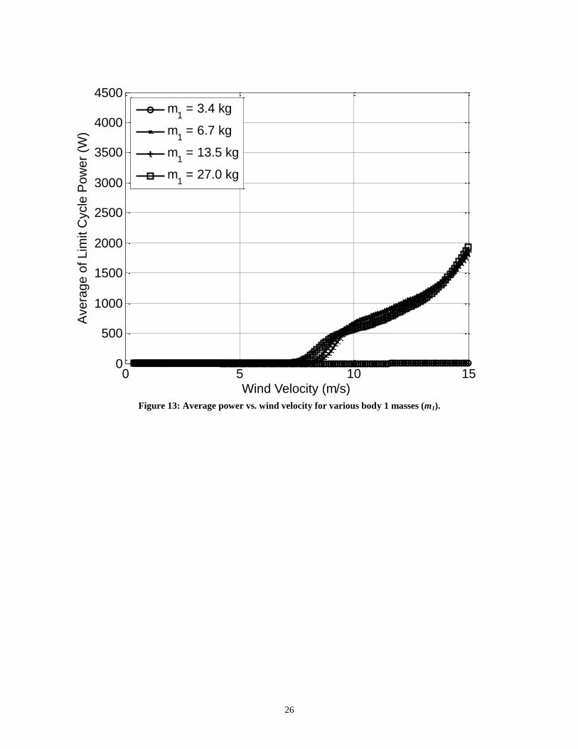
Parametric trade studies about a nominal scenario are presented in Figure 12 through Figure 19 to demonstrate

general trends in power vs. WF physical parameters. In all of these plots, power appears to grow unbounded with

wind speed. In reality, the structural limits of the system would dictate the maximum power output, but these were

not modeled in the present study. The slope of the power curve near the cut-in velocity is also quite large. For

variable wind speeds, this may cause high power fluctuations. However, the WF can be tuned to achieve a limit

cycle over several seconds, thus reducing this potential for high fluctuations. Figure 12 shows the variation of the

average limit cycle power with the mass of the airfoil. The cut-in speed for power generation is significantly lower

when the airfoil mass is decreased. This could prove useful to tuning a WF design to a specific installation site with

known average wind speeds. For sites with lower average wind speeds, it would be desirable to have a very low cut-

in speed. From Figure 13, we can see that the mass of body 1 has the opposite effect on cut-in speed; a larger spacer

mass yields a lower cut-in speed. From these two plots, a good WF design would have a relatively heavy spacer

(body 1) and light airfoil weight determined by the required cut-in speed.

Figure 14 shows the variation of average power with the moment of inertia of body 2. Here, the moment of

inertia is normalized with the maximum possible moment of inertia, given the c.g. and mass of the nominal case.

The slope of the power curve at cut-in goes as the airfoil moment of inertia, but the peak power at high wind

velocities is inversely related to the same.

Figure 15 through Figure 17 show the variation of average power with hinge stiffness, hinge damping, and mast

damping, respectively. Larger stiffness generally equates to more power in an approximately linear relationship.

However, it should be noted that higher stiffness also means lower amplitude oscillations of higher frequency. While

this does produce more power, as the amplitude of oscillation diminishes, the risk of staying within the overrunning

clutches’ deadband range becomes greater, so the generator would not be able to extract the power captured by the

system. As expected, increasing the damping of the mast and hinge decreases power until a point where zero power

is produced. The system cannot achieve a limit cycle if there is too much damping because there is too much energy

dissipating from the system to balance the energy input from the wind. The hinge damping, Ch, has a similar effect

on the cut-in speed as the mass of the airfoil. Therefore, this value can also be used to optimize the system for

efficient power output at a particular location.

12

Figure 18 and Figure 19 show the variation of the average power with the non-dimensional body 2 pivot location

(p2) and the non-dimensional body 2 c.g. location (l2). Power increases as the pivot location moves closer to the c.g.,

and also as the c.g. moves forward of the aerodynamic center (0.25c2). These parameters also affect the cut-in speed,

and so can be adjusted in combination with the others discussed previously to tune cut-in speed.

IV. Conclusions

Wind fins provide an alternative, avian friendly and aesthetically different alternative to traditional wind

turbines. The devices work by dynamically designing the system to flutter such that a stable limit cycle is achieved

that extracts substantial power. Equally sized WFs and HAWTs provide comparable output power. A unique feature

of WFs is the rectangular geometry of the aerodynamic surfaces of the device which make them ideally suited to

narrow passages with high winds, such as between high-rise buildings. Power output of the device follows normal

trends of wind energy machines where under the cut in speed zero power is output. However, the cut-in speed is

higher than typical HAWTs. Beyond the cut in speed power output rapidly increases. Power output is a strong

function of the relative mass of the components of the system and the stiffness and damping properties of the

connections. To maximize the energy extraction capability, the ideal WF design is constructed of light weight

materials with low damping.

V. Acknowledgements

The authors would like to thank Professor Lakshmi Sankar for valuable comments and suggestions regarding the

unsteady aerodynamic model and power comparisons in this work. We would also like to thank the reviewers, who

provided valuable advice on improving the aerodynamic model and the presentation of the results.

VI. References

1. Ahmadi, G., “Aeroelastic wind energy converter,” Energy Conversion, Vol. 18, No. 2, 1978, pp. 115-120.

2. Bielawa, R. L., “Development of an oscillating-vane concept as an innovative wind-energy-conversion system,”

United Technologies Research Center, 1982.

3. McKinney, W., and DeLaurier, J., “The Wingmill: an oscillating-wing windmill,” Journal of Energy, Vol. 5,

No. 2, 1981, pp. 109–115.

13

4. Kinsey, T., and Dumas, G., “Parametric study of an oscillating airfoil in a power-extraction regime,” AIAA

Journal, Vol. 46, No. 6, 2008, pp. 1318–1330.

5. Ward, L., "Windbelt, cheap generator alternative, set to power third world," Popular Mechanics Magazine, Nov.

2007.

6. Morris, D. C., “Wind Fin: articulated, oscillating wind power generator,” WIPO Patent WO/2006/093790, Feb.

24, 2006.

7. Durand, W. F. (Ed.), Aerodynamic Theory, Sec. E., Vol. II, Dover Publications, New York, 1963, p. 50.

8. Peters, D. A., Karunamoorthy, S., and Cao, W., “Finite state induced flow models part I: two-dimensional thin

airfoil,” Journal of Aircraft, Vol. 32, No. 2, 1995, pp. 313–322.

9. Hansen, M. H., Gaunaa, M., Madsen, H. A., “A Beddoes-Leishman type dynamic stall model in state-space and

indicial formulations,” Risø National Laboratory, Roskilde, Denmark, 2004.

10. Sheldahl, R. E., Klimas, P. C., “Aerodynamic characteristics of seven symmetrical airfoil sections through 180-

degree angle of attack for use in aerodynamic analysis of vertical axis wind turbines,” Sandia National

Laboratories, 1981.

11. Bergey Windpower Co., Bergey XL.1 Specification Sheet [Web]. Retrieved from

http://www.bergey.com/Products/XL1.Spec.pdf

14

Figure 1: Side view of WF configuration (not to scale).

Vw

w = 2.4994 m

c2 = 0.9144 m

c1 = 0.3048 m

15

Figure 2: Top view of WF configuration.

Vw

II

IJ

1

2

w

Mast

Hinge Body 1

Body 2

2BJ

2BI

h

16

-150 -100 -50 0 50 100 150-2.5

-2

-1.5

-1

-0.5

0

0.5

1

1.5

2

2.5

(deg)

cl,

cd

cl

cd

Figure 3: Section lift and drag coefficients for NACA 0012 airfoil at Re=10,000 [Sheldahl & Klimas (1981)].

17

-4 -3 -2 -1 0 1 2 3 4-4

-3

-2

-1

0

1

2

3

4

-1.5 -1 -0.5 0 0.5 1 1.5-1.5

-1

-0.5

0

0.5

1

1.5

-1.5 -1 -0.5 0 0.5 1 1.5-1.5

-1

-0.5

0

0.5

1

1.5

A

B C

Figure 4: WF top view snapshots of oscillation at limit cycle; (a) full period [all dimensions accurate]; (b)

upstroke half-period [dimensions altered for better viewing]; (c) downstroke half-period

[dimensions altered for better viewing] (Vw = 11.176 m/s).

Vw

1 2

1 2

17.1 , 13.1 ,

0.0 deg/s, 9.3 deg/s

1 2

1 2

17.1 , 13.1 ,

0.0 deg/s, 9.3 deg/s

1 2

1 2

17.1 , 13.1 ,

0.0 deg/s, 9.3 deg/s

1 2

1 2

17.1 , 13.1 ,

0.0 deg/s, 9.3 deg/s

18

0 5 10 15 20-20

-10

0

10

20

1 (

deg)

0 5 10 15 20-20

-10

0

10

20

Time (sec)

2 (

deg)

Figure 5: WF angles vs. time (Vw = 11.176 m/s).

19

0 5 10 15 20-10

-5

0

5

10d

1/d

t (r

ad/s

)

0 5 10 15 20-5

0

5

Time (sec)

d

2/d

t (r

ad/s

)

Figure 6: WF angular rates vs. time (Vw = 11.176 m/s).

20

-15 -10 -5 0 5 10 15-300

-200

-100

0

100

200

300

2 (deg)

d

2/d

t (d

eg/s

ec)

Figure 7: θ2 phase portrait (Vw = 11.176 m/s).

Start

End

21

0 5 10 15 200

200

400

600

800

1000

1200

1400

1600

1800

2000

Time (sec)

Pow

er

(W)

instantaneous power

average of limit cycle power

Figure 8: Power output vs. time (Vw = 11.176 m/s).

22

0 5 10 15 20-20

-10

0

10

20A

ngle

of A

ttack,

(deg)

0 5 10 15 20-2

-1

0

1

2

Inflow

,

0 (

m/s

)

Time (sec)

Figure 9: Airfoil angle of attack and inflow vs. time (Vw = 11.176 m/s).

23

-20 -15 -10 -5 0 5 10 15 20

-1

0

1

CL

Quasi-Static Model

Dynamic Stall Model

-20 -15 -10 -5 0 5 10 15 20-0.5

0

0.5

CD

Angle of Attack, (deg)

Figure 10: Airfoil lift and drag coefficients vs. angle of attack (Vw = 11.176 m/s). Dynamic stall coefficients are

shown at limit cycle only.

24

-30 -20 -10 0 10 20 30-500

-400

-300

-200

-100

0

100

200

300

400

500

1 (deg)

d

1/d

t (d

eg/s

)

Figure 11: θ1 phase portrait for various initial conditions (Vw = 11.176 m/s).

Start

End

25

0 5 10 150

500

1000

1500

2000

2500

3000

3500

4000

4500

Wind Velocity (m/s)

Avera

ge o

f Lim

it C

ycle

Pow

er

(W)

m2 = 16.9 kg

m2 = 33.9 kg

m2 = 101.7 kg

Figure 12: Average power vs. wind velocity for various airfoil masses (m2).

26

0 5 10 150

500

1000

1500

2000

2500

3000

3500

4000

4500

Wind Velocity (m/s)

Avera

ge o

f Lim

it C

ycle

Pow

er

(W)

m1 = 3.4 kg

m1 = 6.7 kg

m1 = 13.5 kg

m1 = 27.0 kg

Figure 13: Average power vs. wind velocity for various body 1 masses (m1).

27

0 5 10 150

500

1000

1500

2000

2500

3000

3500

4000

4500

Wind Velocity (m/s)

Avera

ge o

f Lim

it C

ycle

Pow

er

(W)

I2z

= 0.50*(I2z

)max

I2z

= 0.75*(I2z

)max

I2z

= 1.00*(I2z

)max

Figure 14: Average power vs. wind velocity for various airfoil moment of inertias (I2z), where (I2z)max is the

maximum moment of inertia possible for a give mass (m2) and c.g location (l2*c2).

28

0 5 10 150

500

1000

1500

2000

2500

3000

3500

4000

4500

Wind Velocity (m/s)

Avera

ge o

f Lim

it C

ycle

Pow

er

(W)

Kh = 423.2 N-m/rad

Kh = 846.4 N-m/rad

Kh = 1692.7 N-m/rad

Figure 15: Average power vs. wind velocity for various hinge stiffness (Kh).

29

0 5 10 150

500

1000

1500

2000

2500

3000

3500

4000

4500

Wind Velocity (m/s)

Avera

ge o

f Lim

it C

ycle

Pow

er

(W)

Ch = 0.5 N-m-s/rad

Ch = 1.0 N-m-s/rad

Ch = 1.5 N-m-s/rad

Figure 16: Average power vs. wind velocity for various hinge damping (Ch).

30

0 5 10 150

500

1000

1500

2000

2500

3000

3500

4000

4500

Wind Velocity (m/s)

Avera

ge o

f Lim

it C

ycle

Pow

er

(W)

Cp = 0.5 N-m-s/rad

Cp = 1.0 N-m-s/rad

Cp = 1.5 N-m-s/rad

Figure 17: Average power vs. wind velocity for various mast damping (Cp).

31

0 5 10 150

500

1000

1500

2000

2500

3000

3500

4000

4500

Wind Velocity (m/s)

Avera

ge o

f Lim

it C

ycle

Pow

er

(W)

p2 = 0.05

p2 = 0.10

p2 = 0.17

p2 = 0.24

Figure 18: Average power vs. wind velocity for various non-dimensional airfoil pivot locations (p2).

32

0 5 10 150

500

1000

1500

2000

2500

3000

3500

4000

4500

Wind Velocity (m/s)

Avera

ge o

f Lim

it C

ycle

Pow

er

(W)

l2 = 0.18

l2 = 0.20

l2 = 0.22

l2 = 0.24

l2 = 0.25

Figure 19: Average power vs. wind velocity for various non-dimensional airfoil c.g. locations (l2).