WIND PARAMETERS OF TEXAS TECH UNIVERSITY FIELD SITE

by

CHEE VUI CHOK, B.S. in C.E.

A THESIS

IN

CIVIL ENGINEERING

Submitted to the Graduate Faculty of Texas Tech University in

Partial Fulfillment of the Requirements for

the Degree of

MASTER OF SCIENCE

IN

CIVIL ENGINEERING

August, 1988

AJ 0 • ' ' • ACKNOWLEDGEMENTS

I would like to express my sincere gratitude and thanks to my committee

chairman, Dr. Kishor C. Mehta, for his guidance, encouragement and constructive

criticism throughout the course of this research. Special thanks are extended to

my thesis committee members, Dr. James R. McDonald and Richard E. Peterson,

for their valuable suggestions and comments.

Financial support by the National Science Foundation through Grant No.

CES8611601 and Civil Engineering Department is acknowledged and appreciated.

Deepest appreciation is reserved for my family. I am grateful to my parents and

my brother, Chee Leong, for their unending support in countless ways. Without

their help, I would not have been able to achieve what I have today.

Acknowledgements would be incomplete without expressing my utmost appre­

ciation to the pioneering members of the Field Experiment team, Basilio Lakas,

Marc Levitan and Howard Ng, for the exemplary team work and enviable fun

we share in this project. Marc Levitan's help in my analysis work is greatly

appreciated.

11

TABLE OF CONTENTS

ACKNOWLEDGEMENTS ii

ABSTRACT v

LIST OF TABLES vi

LIST OF FIGURES vii

CHAPTER

I. INTRODUCTION 1

II. LITERATURE REVIEW FOR CURRENT ENGINEERING PRACTICE 4

Stationarity 5 Atmospheric Stability 7 Wind Profile 9

Power Law 9 Logarithmic Law 9

Turbulence Intensity 12 Integral Scale of Turbulence 14

III. METEOROLOGICAL TOWER INSTRUMENTATION 19

Field Site and Terrain 19 Northeast Terrain 21 Southeast Terrain 21 Southwest Terrain 21 Northwest Terrain 25

Meteorological Tower 25 Instrument Boom 28

Instrumentation 30 Horizontal Wind Measurement System 30 Temperature Measurement System 34 Relative Humidity Measurement System 36 Barometric Pressure Measurement System 37

Data Acquisition System 37

IV. CALIBRATION OF METEOROLOGICAL INSTRUMENTS 39

Anemometer 39 \Mnd Vane 42

111

Temperature Sensor 43 Relative Humidity Sensor 47 Barometric Pressure Sensor 47 Cable Effect 49

V. ANALYSIS OF FIELD DATA 51

Time History 54 Stationarity 57 Descriptive Statistics 66 Wind Profile Parameters 69

Power Law Parameter 69 Logarithmic Law Parameters 71

Terrain Characterization 74 Turbulence Intensity 77 Longitudinal Integral Scale of Turbulence 80

VI. CONCLUSIONS AND RECOMMENDATIONS 85

Conclusions 85 Recommendations 86

LIST OF REFERENCES 88

IV

ABSTRACT

Wind parameters obtained from field data are generally simulated in wind

tunnel for studying wind effects on structures. The result of the wind tunnel study

depends on the reliability of field wind parameters and the simulation technique.

The objective of this study is to assess wind parameters from field data.

The National Science Foundation has sponsored a project at the Texas Tech

University Wind Engineering Research Field Laboratory to study wind effects on

low-rise building. Wind pressure and meteorological data are collected on the

test building and meteorological tower respectively. Meteorological data which

include wind speed, wind direction, temperature, barometric pressure and rela­

tive humidity data, are measured at four levels of the tower. Wind speed, wind

direction and temperature data are used for assessment of wind parameters and

characterization of terrain.

A total of 63, 15-minute duration each, records are collected. Of these, 31

records are found to be suitable for analysis. These 31 records are analyzed to

determine wind profile parameters for both power and logarithmic laws, turbu­

lence intensity and longitudinal integral scale of turbulence. The wind profile

parameters, mean wind directions and terrain features are used to characterize

the field site terrain. Results of the analysis are presented in this report.

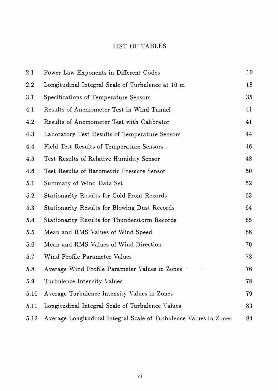
LIST OF TABLES

2.1 Power Law Exponents in Different Codes 10

2.2 Longitudinal Integral Scale of Turbulence at 10 m 18

3.1 Specifications of Temperature Sensors 35

4.1 Results of Anemometer Test in Wind Tunnel 41

4.2 Results of Anemometer Test with Calibrator 41

4.3 Laboratory Test Results of Temperature Sensors 44

4.4 Field Test Results of Temperature Sensors 46

4.5 Test Results of Relative Humidity Sensor 48

4.6 Test Results of Barometric Pressure Sensor 50

5.1 Summary of Wind Data Set 52

5.2 Stationarity Results for Cold Front Records 63

5.3 Stationarity Results for Blowing Dust Records 64

5.4 Stationarity Results for Thunderstorm Records 65

5.5 Mean and RMS Values of Wind Speed 68

5.6 Mean and RMS Values of Wind Direction 70

5.7 Wind Profile Parameter Values 73

5.8 Average Wind Profile Parameter Values in Zones ' 76

5.9 Turbulence Intensity Values 78

5.10 Average Turbulence Intensity Values in Zones 79

5.11 Longitudinal Integral Scale of Turbulence Values 83

5.12 Average Longitudinal Integral Scale of Turbulence Values in Zones 84

VI

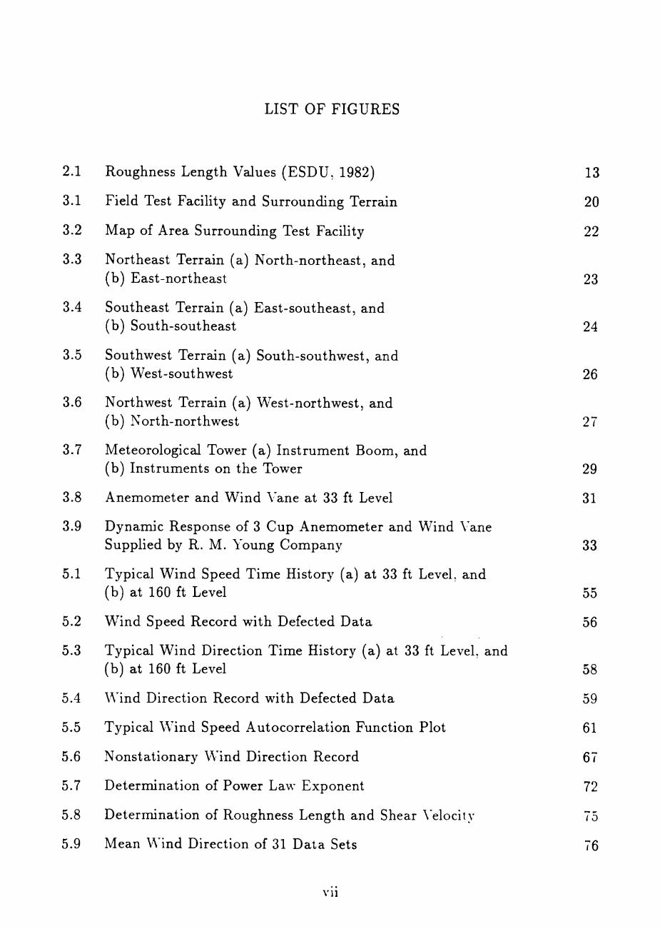
LIST OF FIGURES

2.1 Roughness Length Values (ESDU, 1982) 13

3.1 Field Test Facility and Surrounding Terrain 20

3.2 Map of Area Surrounding Test Facility 22

3.3 Northeast Terrain (a) North-northeast, and (b) East-northeast 23

3.4 Southeast Terrain (a) East-southeast, and (b) South-southeast 24

3.5 Southwest Terrain (a) South-southwest, and (b) West-southwest 26

3.6 Northwest Terrain (a) West-northwest, and (b) North-northwest 27

3.7 Meteorological Tower (a) Instrument Boom, and

(b) Instruments on the Tower 29

3.8 Anemometer and Wind Vane at 33 ft Level 31

3.9 Dynamic Response of 3 Cup Anemometer and Wind Vane Supplied by R. M. Young Company 33

5.1 Typical Wind Speed Time History (a) at 33 ft Level, and

(b) at 160 ft Level 55

5.2 Wind Speed Record with Defected Data 56

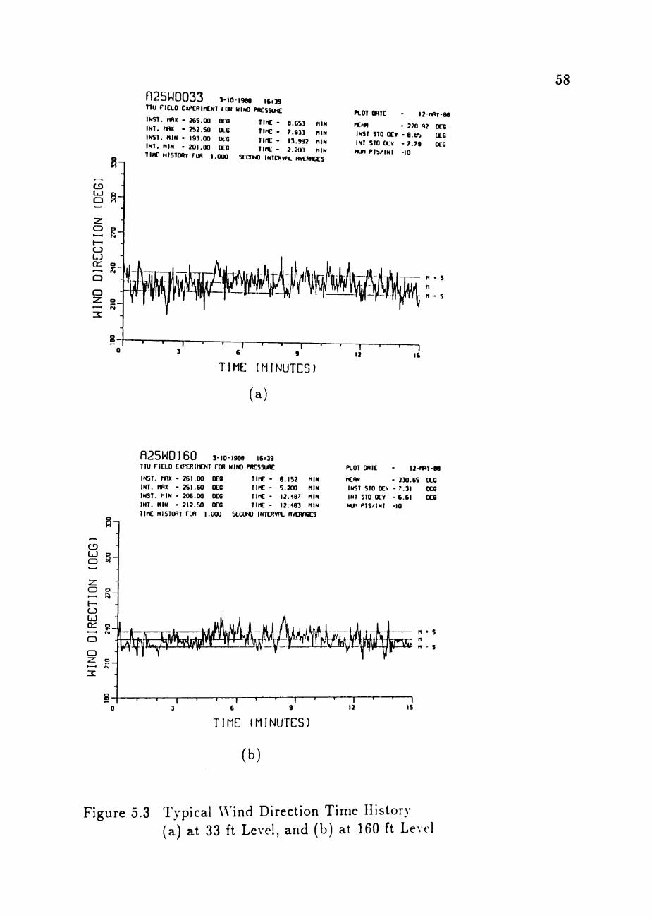
5.3 Typical Wind Direction Time History (a) at 33 ft Level, and

(b) at 160 ft Level 58

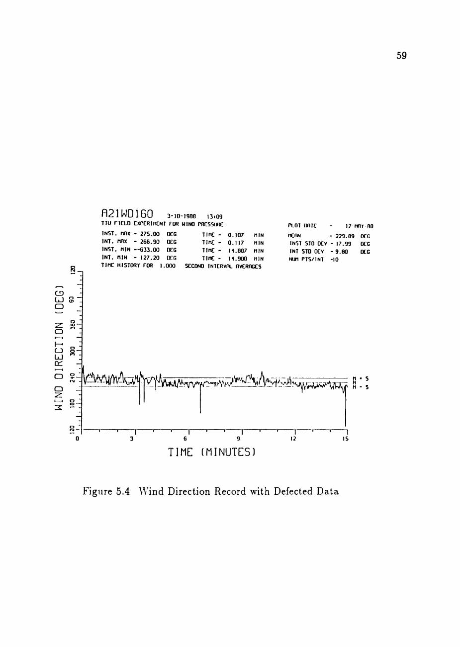
5.4 Wind Direction Record with Defected Data 59

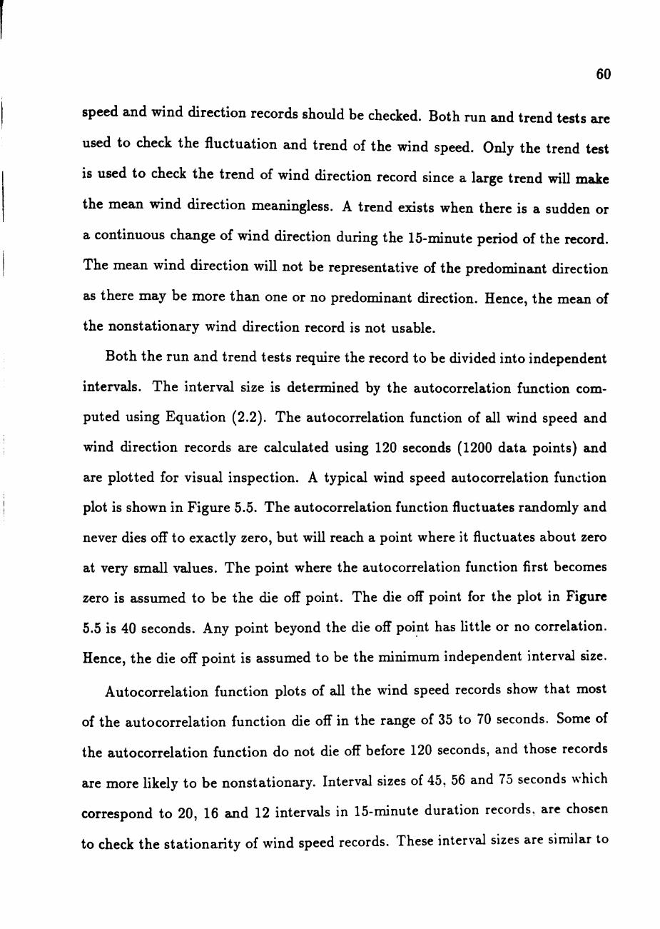
5.5 Typical Wind Speed Autocorrelation Function Plot 61

5.6 Nonstationary Wind Direction Record 67

5.7 Determination of Power Law Exponent 72

5.8 Determination of Roughness Length and Shear \'elocity 75

5.9 Mean Wind Direction of 31 Data Sets 76

v i i

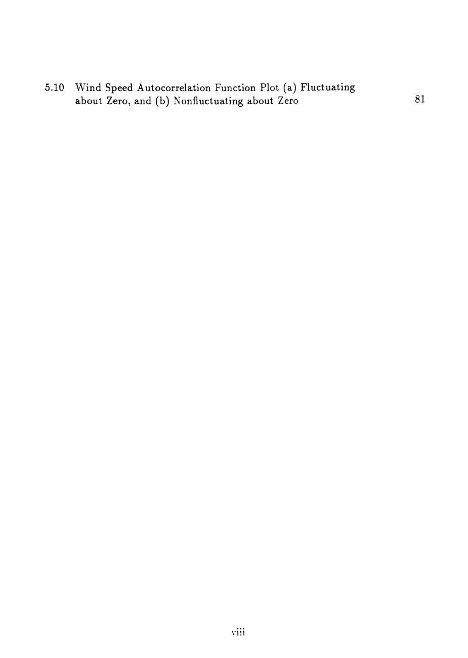
5.10 Wind Speed Autocorrelation Function Plot (a) Fluctuating about Zero, and (b) Nonfluctuating about Zero 81

V l l l

CHAPTER I

INTRODUCTION

Winds in the atmospheric boundary layer (ABL) have significant effects on

the design of structures. Wind forces can damage or even destroy structures.

The extreme winds are of particular interest to structural engineers as structures

have to be designed to prevent collapse. The turbulent nature of wind makes it

difficult to assess the effects of wind on structures. Assessment of turbulence and

other characteristics of wind from field data is necessary to understand the nature

of wind. This understanding of nature of wind will assist in simulation of wind

fiow in the wind tunnel where in-depth study of wind effects on structures can

be done. Only properly simulated wind flow can provide reliable results in wind

tunnels.

Simulation of wind flow requires the effect of test site terrain to be modeled

as the wind flow and the turbulence of the wind are affected by the roughness of

the terrain. Wind flow close to the ground in the field is obstructed by the terrain

roughness, causing turbulent wind with reduced wind speed. As height increases

in the ABL, the wind speed increases and turbulence of wind decreases because

the effect of terrain roughness reduces with height. It is important to assess wind

parameters in the ABL which depend on the terrain roughness.

Proper modeling of the ABL characteristics in the wind tunnel requires cor­

rect simulation of wind profile and turbulence parameters. Only correct simu­

lation can provide realistic model results in term of wind loading. Simulation

of wind profile and turbulence intensity are sufficient for mean load experiment.

Simulation of longitudinal integral scale of turbulence is required in addition to

1

the wind profile and turbulence intensity for unsteady load modeling of low-rise

buildings (Surry, 1979). An incorrect longitudinal integral scale of turbulence

gives unreliable model results.

At present, wind tunnel technology for low-rise building is not fully developed.

The pressure coefficients for low-rise buildings obtained from the wind tunnel are

questionable because of difficulties in scaling the model and in simulating wind

parameters close to the ground. Knowledge of wind characteristics from field data

is necessary to improve modeling for low-rise buildings in wind tunnel.

The well-known fuU scale wind pressure experiment for low-rise building con­

ducted at Aylesbury, England, collected wind and pressure data on a test building

(Eaton and Mayne, 1974). In this experiment, wind data up to 10 m (32.8 ft)

were collected and analyzed. Simulation of this experiment in wind tunnel showed

that a change of wind profile slope occurred at a height of about 15 m because

of hedges around the test building (Surry and Vickery, 1982). But the field data

extended only up to 10 m. There was difficulty in matching the wind tunnel and

the full scale results. Without proper establishment of wind parameters in the

field, it is difficult to duplicate the results in the wind tunnel.

The need for better understanding of wind effects on low-rise buildings has

led to a research project on a full scale wind study in the field at Texas Tech

University. The National Science Foundation has sponsored the project to acquire

wind and associated pressures on a building in the field. This project provides

an opportunity to study wind parameters in the bottom layer of the ABL and to

assess the wind parameters as they are affected by terrain. Instruments for wind

speed, wind direction, temperature, relative humidity and barometric pressure,

are installed at various levels of a 160 ft meteorological tower. .A. computer

controlled data acquisition system is housed inside the data acquisition room.

Data collected at the site is used to assess wind parameters.

The objectives of this study are to assess wind parameters for the Texas Tech

University field site. These parameters will be used to analyze building pressure

data collected at the test site as well as to assist simulation of winds in wind

tunnel studies. Specific objectives in this research are :

1. the assembly of the meteorological tower instrumentation,

2. the calibration of the instrumentation, and

3. the characterization of the field site for wind profile, turbulence intensity

and longitudinal integral scale of turbulence.

The following chapter contains an overview of the literature review for current

engineering practice concerning stationarity of time series, atmospheric stability,

wind profile, turbulence intensity and integral scale of turbulence. Description

of the field site and the meteorological tower instrumentation are presented in

Chapter III. Methodology and results of calibration of the instrumentation are

presented in Chapter IV. Chapter V contains the analysis of the field data which

includes stationarity check, and assessment of the wind profile, turbulence inten­

sity and longitudinal integral scale of turbulence parameters. Conclusions of this

study are presented in Chapter VI.

CHAPTER II

LITERATURE REVIEW FOR CURRENT

ENGINEERING PRACTICE

Large scale motion of the atmosphere is derived from solar energy which is

transmitted to the earth's surface. The movement of air in the atmosphere is

termed wind. At sufficient height above the ground surface, frictional forces

caused by the ground surface roughness become negligible and the wind speed

is essentially constant and is called gradient wind. The height at which the

gradient wind exists is termed gradient height. Between the earth's surface and

the gradient height, wind is affected by frictional forces (mechanical turbulence),

and this region is called atmospheric boundary layer (ABL). All the earth-bound

structures are subjected to complex wind turbulence in the ABL. The vertical

temperature variation which is called thermal gradient also modifies wind in the

ABL; however, major wind effects on structures are associated with strong winds

for which thermal gradient effects are small and generally neglected.

Wind in the ABL is turbulent in nature and fluctuates randomly in time and

space. Fluctuating wind can be assumed to consist of a steady component and

fluctuations about this steady component; these are called mean and turbulence

respectively. Because of its random fluctuating nature, it is essential to use sta­

tistical analysis to define wind parameters.

Statistical analysis of the wind data requires the time series be stationary

before any analysis can be performed. Stationarity of time series, atmospheric

stability and wind parameters which include wind profile, turbulence intensity

and integral scale of turbulence are discussed in this chapter.

Stationarity

A randomly fluctuating time series can be categorized as being either station­

ary or nonstationary. A time series is said to be stationary when its statistical

properties are invariant of time. It is important to assess the stationarity of the

time series because almost all time series analysis procedures in the current prac­

tice assume that the data being analyzed is stationary (Jenkins and Watts, 1968).

If the time series is nonstationary, most of the currently used analysis procedures

are not applicable.

There are two stationary conditions, weakly stationary and strongly station­

ary. A weakly stationary condition exists when the ensemble averaged mean is

invariant of time and the ensemble averaged autocorrelation function is indepen­

dent of starting time (Bendat and Piersol, 1986). Any other stationary situation

is classified as strongly stationary condition. For analysis of wind data, only sta­

tistical parameter, root mean square is used, hence weakly stationary condition

is sufficient.

For a single time series, a slightly different interpretation of stationarity is

needed. Stationarity of a time series means the statistical properties computed

over short time intervals do not vary from one interval to the next, which is usually

referred to as self-stationarity. A time series is said to be self-stationary when the

mean and the autocorrelation function averaged over short time interval do not

vary from interval to interval. The mean and autocorrelation function as given

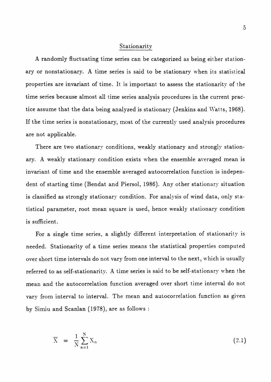
by Simiu and Scanlan (1978), are as follows :

X = ^ i : x „ (2.1) n = l

1 ''•• ''' ^ = ^i (N3;) E (Xn - X)(X„^. - X) (2.2)

where p[r) = the autocorrrelation function at lag r,

X = the mean of the time series,

Xn = the nth data point of the time series,

(T^ — the variance of the time series, and

N = the total number of data point.

The interval length must be carefully chosen so that it represents a true aver­

age properties of the time series. The interval must be statistically independent

(Levitan, 1988). Once the interval length is chosen, the time series is divided into

intervals. The mean and autocorrelation are calculated to examine any variation

from interval to interval.

Practically, computing the autocorrelation function of a large time series for all

the possible lags uses a large amount of computer time. Bendat and Piersol (1986)

have suggested that a time series can be considered self-stationary if the mean

and the autocorrelation function (see Equation (2.2)) at lag equal to zero (mean

square value), contain no trends or variations other than sampHng variations.

Two tests, the run and trend tests are used to check the stationaritv of a

time series. The run test is more powerful for detecting the fluctuating trends,

whereas the trend test is powerful for detecting monotonic trends (Bendat and

Piersol, 1986). It is hypothesized that the sets of mean and mean square value

are independent and self-stationary. The hypothesis is tested at a confidence

level of /? which is usually 90%, 95% or 99%. The hypothesis is accepted if the

number of runs for run test or the number of reverse arrangements for trend tost

fall within the acceptable region. The acceptance of the hypothesis means that

there is insufficient evidence to believe the time series to be self-nonstationary.

Rejection of the hypothesis shows that there is enough evidence to befieve the

time series to be self-nonstationarv.

Atmospheric Stabihty

Three general states of atmospheric stability conditions are defined : neutral,

unstable and stable. Under neutral stability condition, the lapse rate which is

the temperature variation with height, is equal to the dry adiabatic rate, which

is 5.5°F per 1000 ft (Navarra, 1979). Neutral stability condition usually exists

in strong winds where turbulence caused by ground roughness, called mechanical

turbulence, is predominant. Under unstable stability condition, the lapse rate

is greater than the dry adiabatic rate. Air near ground surface is warmer and

less dense than the air above, creating a thermal gradient. The thermal gradient

causes the air to rise rapidly which generates thermal turbulence. The combina­

tion of mechanical and thermal turbulence exists in this condition. Under stable

condition, the lapse rate is less than the dry adiabatic rate. At the extreme, there

is a temperature inversion; typically, the winds are light and a cool dense layer

of air forms above the ground. In stable condition, the mechanical turbulence

may be suppressed. For the extreme wind that cause high loads on buildings, the

atmospheric stability condition is usually neutral where mechanical turbulence is

predominant.

It is desirable to determine the stability conditions at the time of data collec­

tion because the wind profile equation is primarily valid for near neutral stability

condition. The gradient Richardson number. Ri. which indicates the relative

8

importance of thermal to mechanical turbulence, can be used to distinguish the

stability conditions as stable, neutral or unstable depending upon whether its

value is positive, zero or negative respectively. Fichtl (1968) has developed the

following equation to estimate gradient Richardson number at the geometrical

mean height by assuming that the mean wind speed and the temperature are

distributed logarithmically between two levels Zi and Z2. It is represented as :

Ri(ZJ = ^ T(Z,)

T(Z,)-T(Zi) g U(Z,)-U(Zi) - 2

(2.3)

where Ri(Zg) = the gradient Richardson number at the

geometric mean height,

g = the acceleration due to gravity,

T(Z) = the mean temperature at height Z.

Cp = the specific heat of air at constant pressure,

U(Z) = the mean wind speed at bight Z and.

Zg = the geometric mean height (= vZ]Z2)-

The limit of gradient Richardson number for near neutral stability condition

has been suggested by several researchers. Teunissen (1970) and Panofsky (1977)

have suggested |Ri| < 0.03 and |Ri| < 0.01 for neutral stabihty condition respec­

tively. Duchene-MarruUaz (1978) assumed near neutral stability condition when

Ri is between 0.025 and 0.015.

Neutral stability condition is generally assumed to exist by engineers when

the wind speed at 33 ft is higher than 20 mph. ESDU (1982) has suggested that

near neutral stabihty condition exists when the mean hourly wind speed is greater

than 10 mps (22 mph) at the height of 10 m (33 ft).

Wind Profile

Wind profile is the variation of mean wind speed with height above ground.

It is usually represented by power law or logarithmic law.

Power Law

Power law is an empirical equation and is widely used by engineers because

of its simpHcity. It is represented by the following equation (Davenport, 1960) :

Ui /ZiN'^

u; = (z;) (2- )

where Ui, U2 = the wind speeds at height Zi, Z2 respectively, and

a = the power law exponent.

The power law exponent is dependent on ground surface roughness and aver­

aging time. It is suggested by Davenport (1960) that the power law is valid in

near neutral atmospheric stability condition. Typical power law exponent values

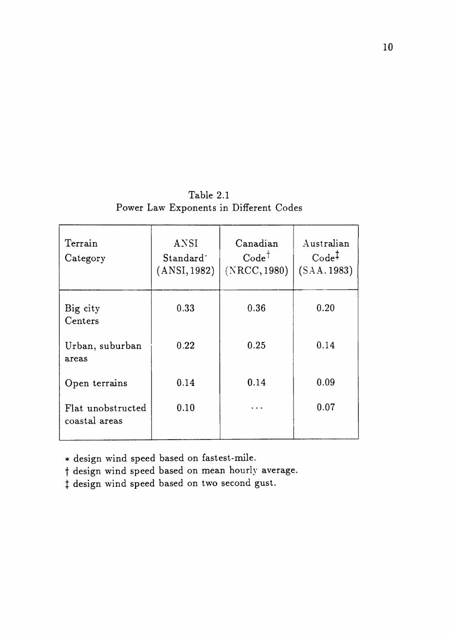
used by various national codes are shown in Table 2.1. The power law exponent

value increases with rougher terrain.

Equation (2.4) is primarily used for tall structures because of its assumed

validity up to the gradient height. However, it has been criticized on the ground

that the power law exponent is not constant, but varies significantly with different

height range above ground (Hansen, 1970).

Logarithmic Law

Logarithmic law is developed from physical laws and is widely accepted by

meteorologists. It can be represented as follows (Simiu, 1973) :

10

Table 2.1 Power Law Exponents in Different Codes

Terrain

Category

Big city Centers

Urban, suburban areas

Open terrains

Flat unobstructed coastal areas

ANSI

Standard' (ANSI, 1982)

0.33

0.22

0.14

0.10

Canadian

CodeT (NRCC,1980)

0.36

0.25

0.14

Australian

Codet (SAA.1983)

0.20

0.14

0.09

0.07

* design wind speed based on fastest-mile. t design wind speed based on mean hourly average. I design wind speed based on two second gust.

11

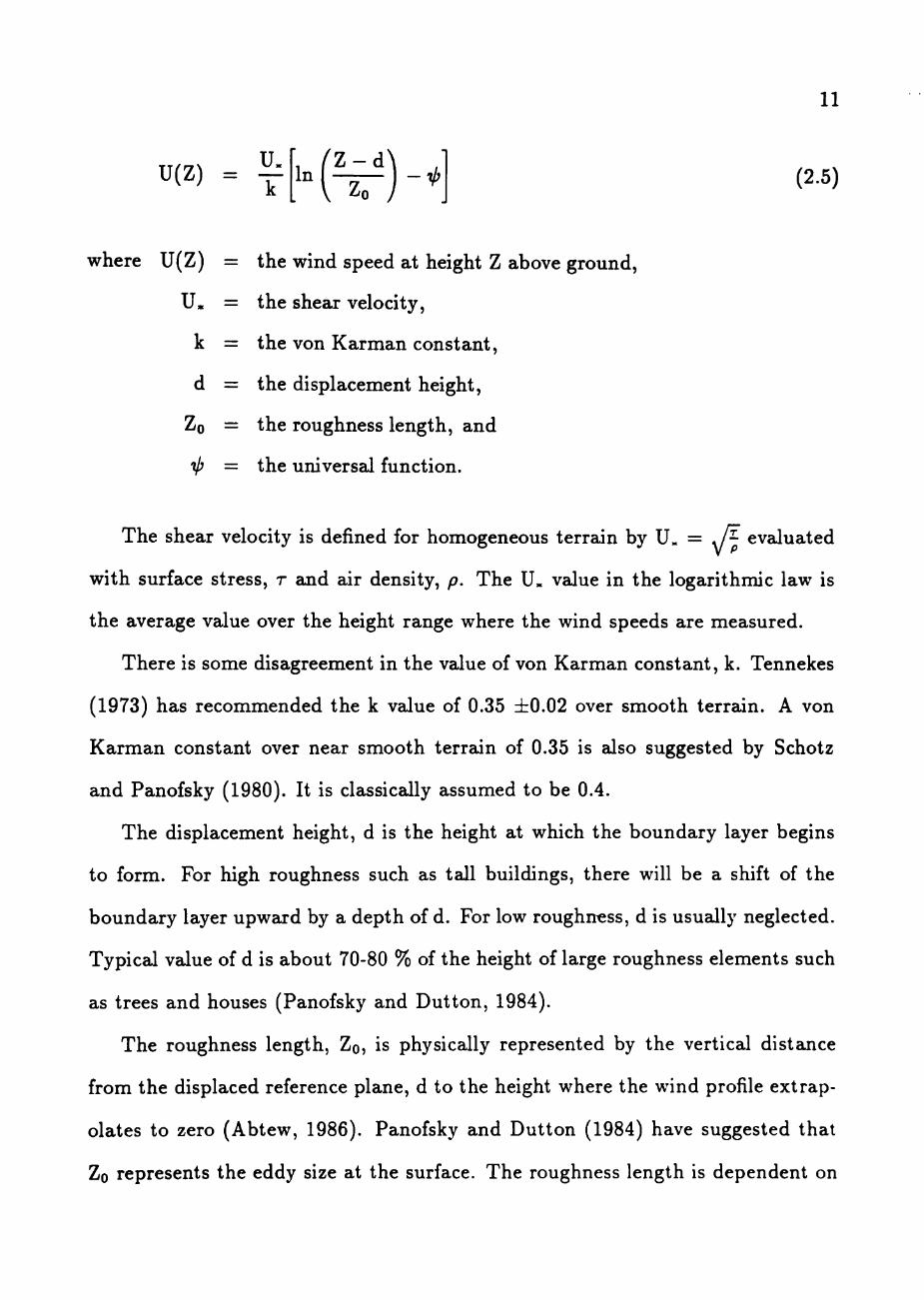
U(Z) = ^ I n l ^ l - ^ (2.5)

where U(Z) = the wind speed at height Z above ground,

U» = the shear velocity,

k = the von Karman constant,

d = the displacement height,

Zo = the roughness length, and

ip = the universal function.

The shear velocity is defined for homogeneous terrain by U. = J^ evaluated

with surface stress, r and air density, p. The U« value in the logarithmic law is

the average value over the height range where the wind speeds are measured.

There is some disagreement in the value of von Karman constant, k. Tennekes

(1973) has recommended the k value of 0.35 ±0.02 over smooth terrain. A von

Karman constant over near smooth terrain of 0.35 is also suggested by Schotz

and Panofsky (1980). It is classically assumed to be 0.4.

The displacement height, d is the height at which the boundary layer begins

to form. For high roughness such as tall buildings, there will be a shift of the

boundary layer upward by a depth of d. For low roughness, d is usually neglected.

Typical value of d is about 70-80 % of the height of large roughness elements such

as trees and houses (Panofsky and Dutton, 1984).

The roughness length, ZQ, is physically represented by the vertical distance

from the displaced reference plane, d to the height where the wind profile extrap­

olates to zero (Abtew, 1986). Panofsky and Dutton (1984) have suggested that

Zo represents the eddy size at the surface. The roughness length is dependent on

12

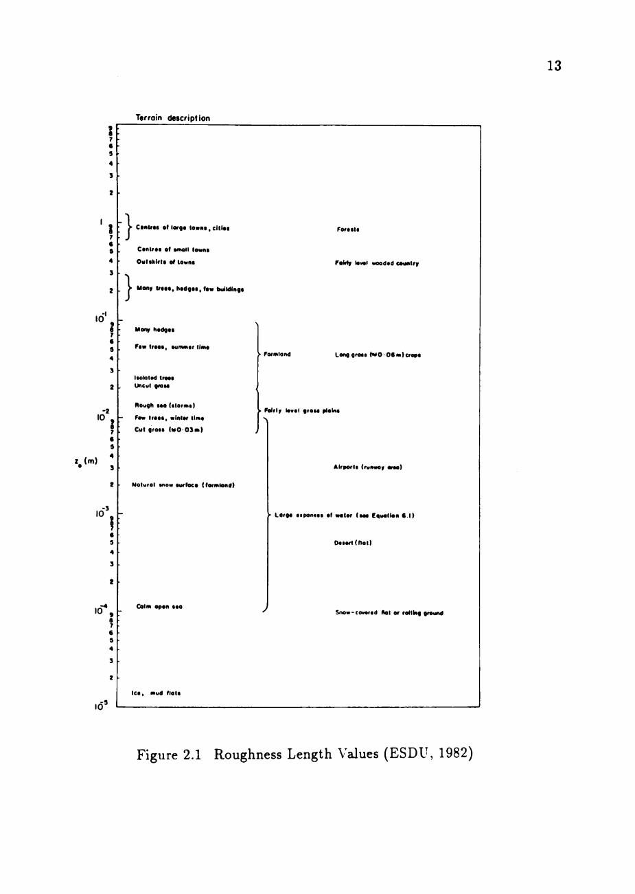
the surface roughness. Typical values of roughness length for different terrains

are shown in Figure 2.1.

The universal function, ij) is included in Equation (2.5) for diabatic condition

where the vertical thermal effects become important comparable to the effects of

mechanical mixing. It is assumed to be zero for neutral stability condition.

The logarithmic law is an excellent representation of wind profile in horizon­

tally homogeneous surface (Simiu, 1973); it is assumed to be vaHd up to about

30-50 m above ground (Simiu and Scanlan, 1978). Garratt (1978) also suggests

that logarithmic law fails at Z < IOZQ. The reason is that condition at this small

height is no longer horizontally homogeneous because of the effects of individual

elements.

Turbulence Intensity

The most commonly used parameter to define turbulence in time domain is

turbulence intensity. It is a measure of the relative ampHtude of the fluctuations

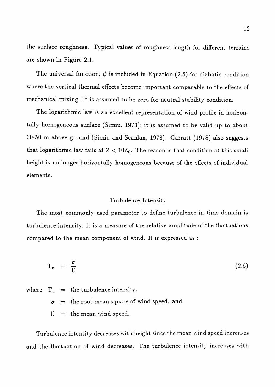
compared to the mean component of wind. It is expressed as :

T. = J (2.6)

where Tu = the turbulence intensity.

a = the root mean square of wind speed, and

U = the mean wind speed.

Turbulence intensity decreases with height since the mean wind speed increases

and the fluctuation of wind decreases. The turbulence intensity increases with

13

Terrain description 9 S 7 • 9 '

% T 6 » 4

3

}

1}

C*«lr«( of lar«« l o a m , ciliat

C*nlr«f of ainall lawnt

OuUklrl* of loon*

Mony I f M t , hadgci, f«« buiMiitft

FOftltt

Foifty l*>«l weodti Muniry

Id' 2 7 e 9 4

-2

10

Mony hodgo*

F t * Iroot, tummtr llm«

Itololcd Iroo* Uncul giOM

Rough u o (ilormi)

Fmr lr««(, winlor llm*

Cul groM ( « 0 ' 0 3 m )

• s

i d \

Nalurol wtoo tuffoco (forntlondl

10 Calm epon t«o

> Fofntlond Lenggroti ttO-Otm)aap»

> Folrly lovol groH ftaint

AlrpOfli (rwMMy oroo)

> La«g« tipontM of I M I M ( M O Couollon C.I)

0«i*f«(nall

y Sno>-co»«r*d Hal or rolling ground

let , mud dolt

Id'

Figure 2.1 Roughness Length Values (ESDU, 1982)

14

averaging time as mean wind speed tends to decrease with increase in averaging

time (Kancharla, 1986).

Integral Scale of Turbulence

Integral scales of turbulence are measures of the average size of turbulence

eddies in appropriate directions (Simiu and Scanlan, 1986). They take the form

of ellipsoids, much elongated in the direction of the mean wind speed. Hence, there

are three integral length scales of turbulence corresponding to the longitudinal,

lateral and vertical fluctuating component of wind.

Reported integral scales of turbulence have displayed a large degree of vari­

ability. Part of this variability is the result of the dependence of integral scales of

turbulence on terrain characteristics, atmospheric stability condition and height

above ground. Considerable variabifity also results from different computation

methods for integral scales (Teunissen, 1980). In general, the sizes of integral

scales of turbulence increase with smoother terrain and height above ground as

ground roughness distorts the formation of large eddies. They decrease slightly

with increasing atmospheric stability (Moore et al., 1985).

Mathematically, the integral scale of turbulence is the integral of the space

correlation function. But the measurement of wind speeds at various spatial lo­

cations are not always possible. Subject to the validity of Taylor's hypc>thesis.

the observed time correlation function at a point can be interpreted as the space

correlation function along the mean wind direction. Taylors hypothesis has ini-

phed that for homogeneous turbulence, if the square of mean wind speed is much

greater than the variance of wind speed (U^ > > a-'), the lime correlation functic»n

can be converted into space correlation function as follows (Taylor. 193S) :

15

X = U t (2.7)

where X = the distance along mean wind direction,

U = the mean wind speed, and

t = the time.

Taylor's hypothesis implies that the turbulence field can be considered as

'frozen' in space and time, and travels past a point with velocity U. The variation

of (T^ with time when the turbulence is viewed from a stationary point is the

same as the variation observed from a point moving across the 'frozen field' with

velocity U in the negative mean wind direction. Lappe and Davidson (1963), had

shown that the Taylor's hypothesis is valid for wavelength ranging from at least

600 to 900 ft as mean wind speed varies from 20 to 30 fps respectively. Panofsky

and Dutton (1984) also suggested that Taylor's hypothesis is valid for weakly

stationary wind data. In this project, the mean square of wind speed, U^ can be

as low as 400 mph squared (mean wind speed of 20 mph) and the variance, cr

can be as high as 25 mph squared (root mean square value of 5 mph). Hence,

the mean square value is at least 16 times greater than the variance value and

it is assumed to satisfy Equation (2.7). As a result, the Taylor's hypothesis is

assumed to be valid.

The validity of Taylor's hypothesis has important consequences for statistical

analysis. The mean and variance measured in time must equal to those measured

in space. Similarly, the autocorrelation function, PS{T) in space and px[''') in

time must be equal. The longitudinal integral scale of turbulence can hence be

estimated as a product of mean wind speed and time scale measured at a point.

The time scale characterizes the average duration of the effect of eddies at a point

16

(ESDU, 1974). It is the area under the autocorrelation function curve of a time

series.

The longitudinal integral scale of turbulence can be represented as follows :

Lx = \] 1°° p(r)dr (2.8)

where Lx = the longitudinal integral scale of turbulence,

U = the mean wind speed, and

p{r) = the autocorrelation function at lag, r.

There are four different methods to evaluate the longitudinal integral scale of

turbulence. The methods are :

1. The direct integration of autocorrelation function method (Teunissen, 1979).

This approach is quite sensitive to the oscillatory behavior of the aotucor-

relation function. A cutoff value is required of time lag.

2. The spectral method (Teunissen, 1979). This method uses the frequency,

fmax at which the power spectrum is the maximum. The product of the

mean wind speed and the inverse of fmax is the longitudinal integral scale of

turbulence.

3. The exponential function method (Teunissen, 1979). This approach assumes

an exponential function. The lag time at which the autocorrelation function

is equal to 1/e (0.368) is multiplied by the mean wind speed to get the

longitudinal integral scale of turbulence.

4. The direct integration of a best fit function method (Mackey and Lo. 1975).

rhe best fit function is usually an exponential function.

Different values of longitudinal integral scale of turbulence at 10 m computed

using different methods by several investigators are shown in Table 2.2. A vari­

ation of the values is observed for different terrains and different computation

methods.

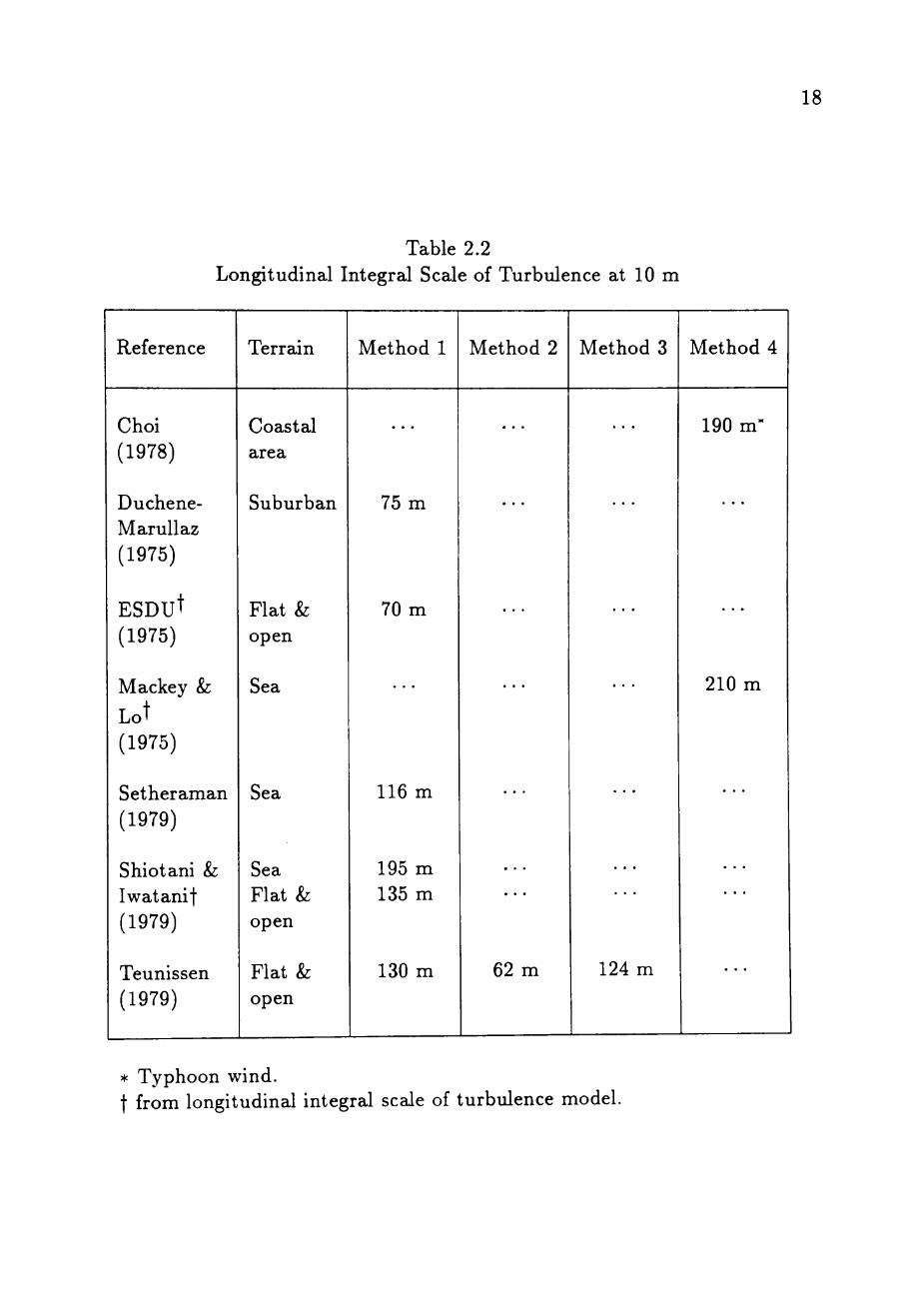
18

Table 2.2 Longitudinal Integral Scale of Turbulence at 10 m

Reference

Choi (1978)

Duchene-Marullaz (1975)

ESDUt (1975)

Mackey &

Lot (1975)

Setheraman (1979)

Shiotani Sz Iwatanif (1979)

Teunissen (1979)

Terrain

Coastal area

Suburban

Flat & open

Sea

Sea

Sea Flat & open

Flat & open

Method 1

75 m

70 m

116 m

195 m 135 m

130 m

Method 2

• • •

62 m

Method 3

o • •

. . .

124 m

Method 4

190 m"

• • •

210 m

. . .

* Typhoon wind. t from longitudinal integral scale of turbulence model.

CHAPTER III

METEOROLOGICAL TOWER

INSTRUMENTATION

The National Science Foundation has sponsored a project to acquire wind

pressure data on a low-rise building. A 30 x 45 x 13 ft rotatable metal building, a

1 0 x 1 0 x 8 ft data acquisition room on a concrete slab and a 160 ft meteorological

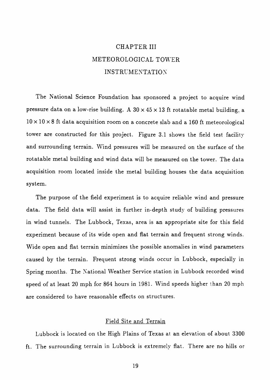
tower are constructed for this project. Figure 3.1 shows the field test facihty

and surrounding terrain. Wind pressures will be measured on the surface of the

rotatable metal building and wind data will be measured on the tower. The data

acquisition room located inside the metal building houses the data acquisition

system.

The purpose of the field experiment is to acquire reliable wind and pressure

data. The field data will assist in further in-depth study of building pressures

in wind tunnels. The Lubbock, Texas, area is an appropriate site for this field

experiment because of its wide open and flat terrain and frequent strong winds.

Wide open and flat terrain minimizes the possible anomalies in wind parameters

caused by the terrain. Frequent strong winds occur in Lubbock, especially in

Spring months. The National Weather Service station in Lubbock recorded wind

speed of at least 20 mph for 864 hours in 1981. Wind speeds higher than 20 mph

are considered to have reasonable effects on structures.

Field Site and Terrain

Lubbock is located on the High Plains of Texas at an elevation of about 3300

ft. The surrounding terrain in Lubbock is extremely flat. There are no hills or

19

20

Figure 3.1 Field Test Facility and Surrounding Terrain

21

valleys within the 20 mile radius of the city. Most of the surrounding land is used

for growing cotton and sorghum. The rest of the land is sparsely populated with

semi-arid vegetation such as short grasses and mesquite trees.

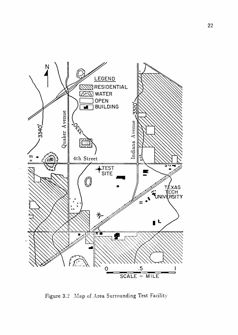
The field site is on the land owned by Texas Tech University. The field test

facihty is on the Antenna Farm, south of 4th Street and half way between Indiana

Avenue and Quaker Avenue as shown in Figure 3.2. General description of the

terrain surrounding the field test facihty is given below.

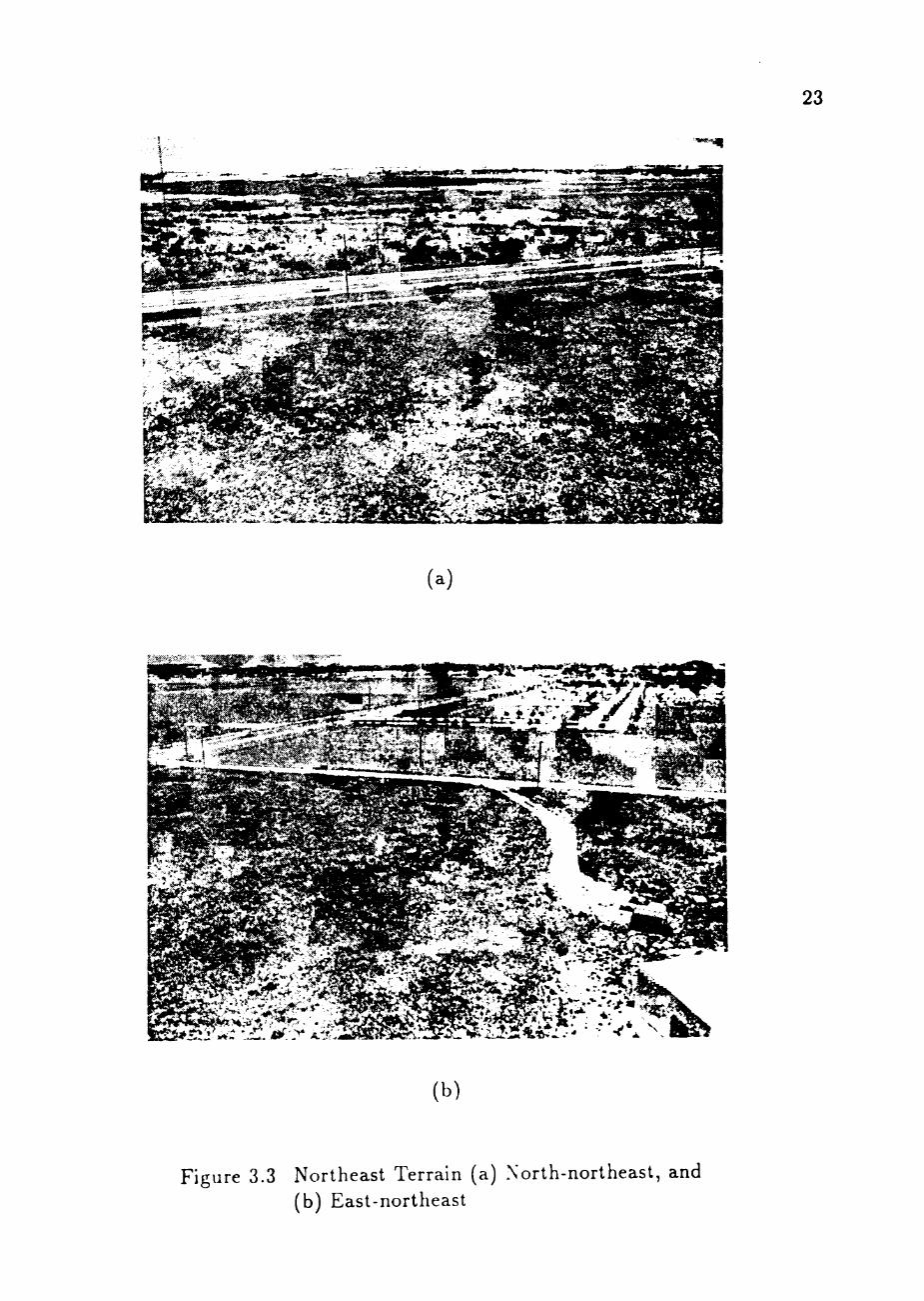
Northeast Terrain

There are residential areas more than 4000 ft away in the azimuth range of 0°

to 80°. The area north of 4th Street in this direction, as shown in Figure 3.3 is

used for growing cotton which is about 2 to 3 ft tall during summer months. The

rest of the area is populated with short grasses.

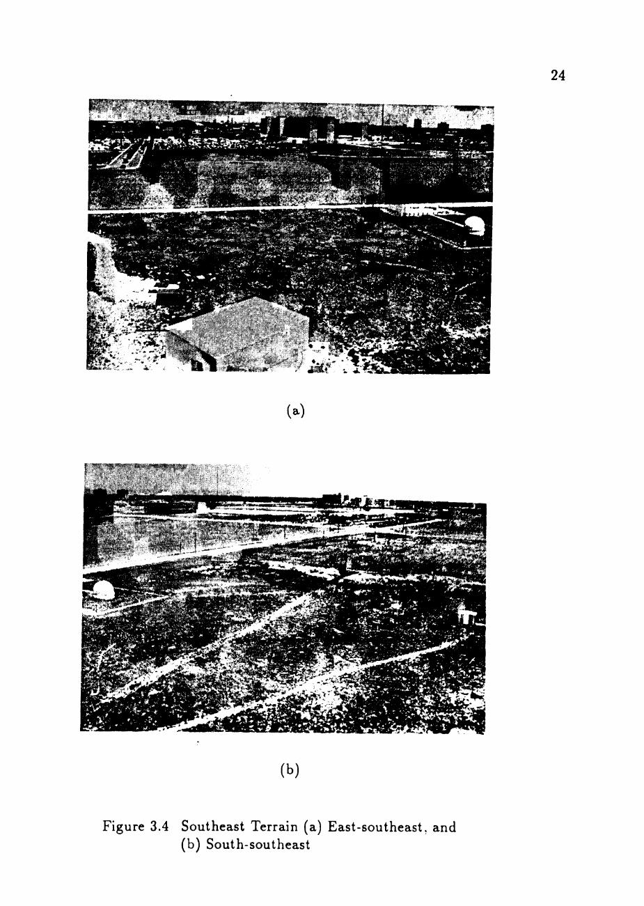
Southeast Terrain

A few big structures are located in the southeast direction as shown in Figure

3.4. A 103 ft tall hospital is 1500 ft away in the azimuth range of 100° to 120°.

The closest structure to the field facility is a 15 ft tall dome-shaped observatory.

It is 200 ft away from the tower at an azimuth of 120°. A power plant in the

azimuth range of 130° to 140° is 1400 ft away. These structures can cause some

interference to the wind flows coming from the southeast.

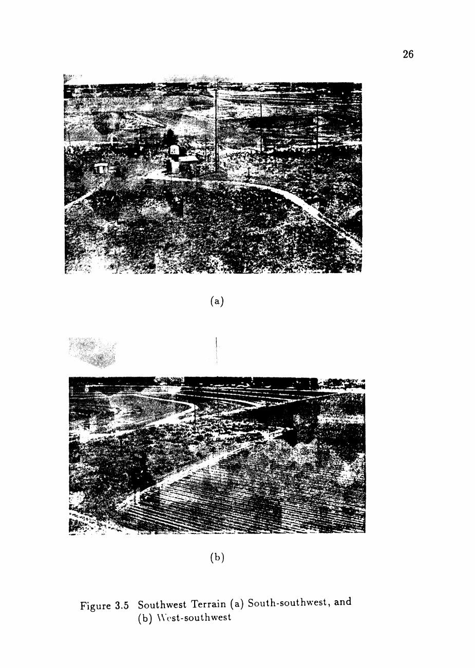
Southwest Terrain

Residential areas begin 2000 ft away in the azimuth range of 180° to 260°. A

10 X 8 X 8 ft power supply shack is 250 ft away at an azimuth of 180°. A larger

22

Figure 3.2 Map of .-Vrea Surrounding Test Facility

23

w » ^

(a)

(b)

Figure 3.3 Northeast Terrain (a) North-northeast, and (b) East-northeast

24

(a)

(b)

Figure 3.4 Southeast Terrain (a) East-southeast, and (b) South-southeast

25

building, 28 x 28 x 26 ft, used for electrical engineering research at an azimuth

of 200° is 250 ft away. There are a few 50 ft high utihty poles around the two

buildings. A large playa lake is about 800 ft away in the azimuth range of 200° to

230°. The playa lake is 800 ft long in the north-south direction and has a width

of 500 ft in the east-west direction. The water surface elevation of the lake is 15 ft

lower than the field test facility elevation. The elevation difference may increase

by another 10 ft during the summer months when the lake dries up. Figure 3.5

shows the southwest terrain.

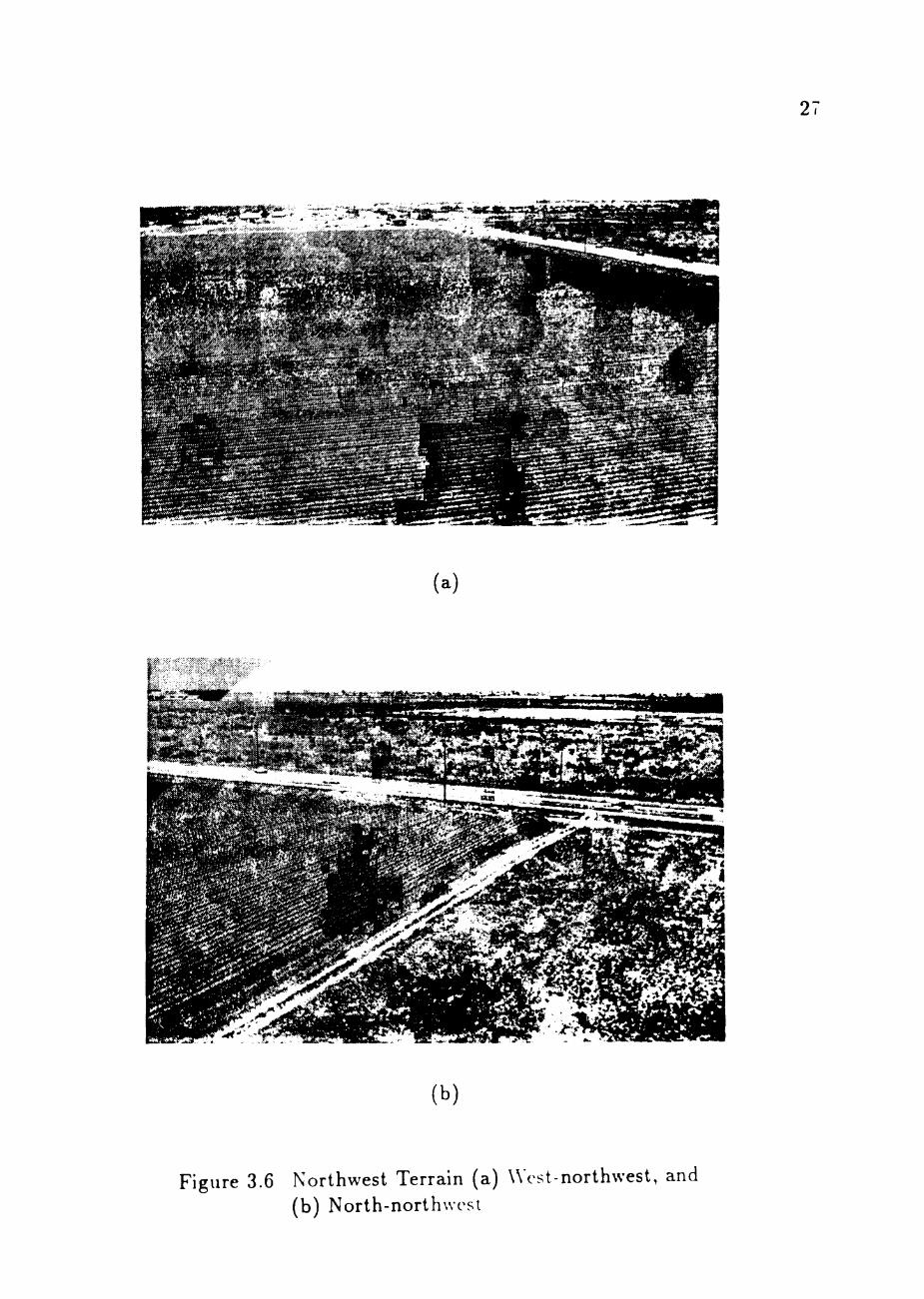
Northwest Terrain

The northwest terrain is open and flat. Three large ponds forming a 600x800

ft rectangle are 2200 ft away in the azimuth range of 330° to 360°. The rest of

the areas north of 4th Street are sparsely populated with 3 to 5 ft tall mesquite

trees. Figure 3.6 shows the northwest terrain.

Meteorological Tower

The meteorological tower is 160 ft high. It is a three-legged truss tower. The

legs are 1.5 ft apart forming an equilateral triangle. The tower are supported by

two sets of guy wires, located at heights of 70 and 130 ft. The guy wire locations

are designed not to interfere with the wind flows measured by instruments at

various levels of the tower. Safety chmb system is installed on the tower for the

safety of the personnel.

The tower is located 150 ft west of the test building. This distance allows the

guy wire anchors which are 104 ft away from the tower, to be kept at a distance

from the test building. The closest guy wire anchor is 10 ft southwest of the

26

(a)

(b)

Figure 3.5 Southwest Terrain (a) South-southwest, and (b) West-southwest

(a)

(b)

Figure 3.6 Northwest Terrain (a) West-northwest, and (b) North-northwost

28

edge of the test building. Possible interference of the guy wires to the wind flows

around the test building is minimized.

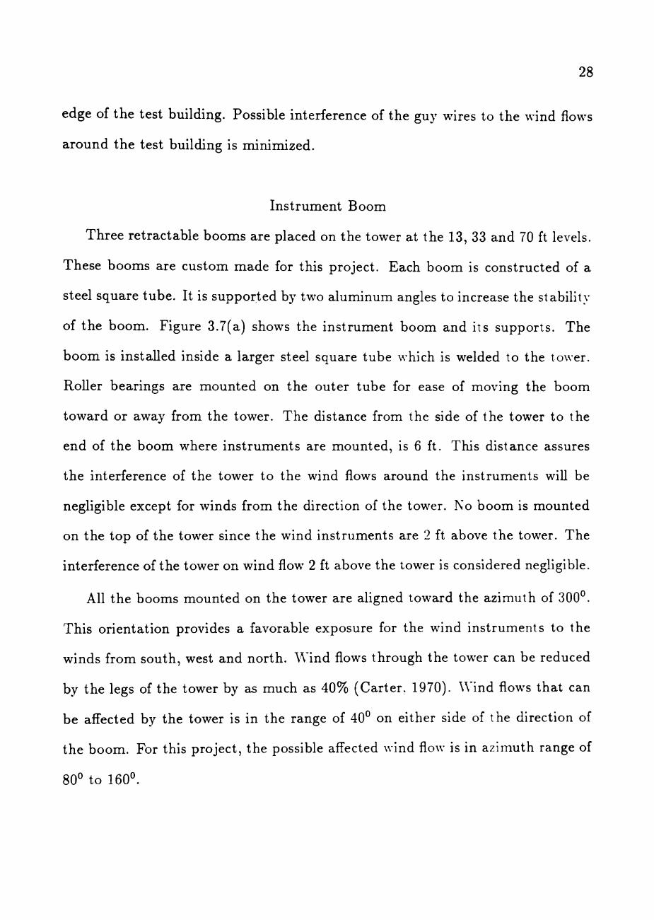
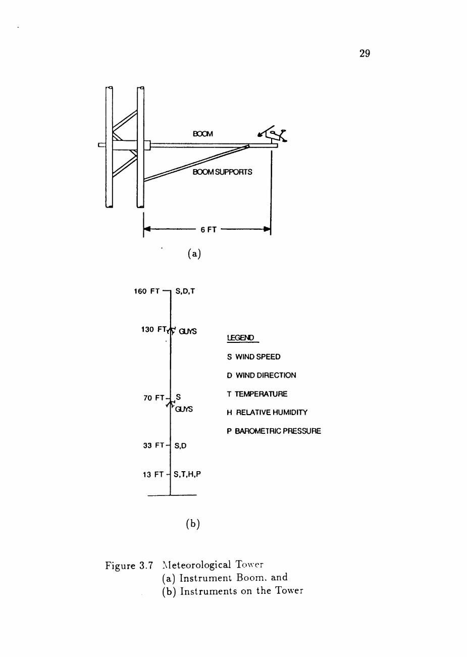
Instrument Boom

Three retractable booms are placed on the tower at the 13, 33 and 70 ft levels.

These booms are custom made for this project. Each boom is constructed of a

steel square tube. It is supported by two aluminum angles to increase the stabihty

of the boom. Figure 3.7(a) shows the instrument boom and its supports. The

boom is instaUed inside a larger steel square tube which is welded to the tower.

RoUer bearings are mounted on the outer tube for ease of moving the boom

toward or away from the tower. The distance from the side of the tower to the

end of the boom where instruments are mounted, is 6 ft. This distance assures

the interference of the tower to the wind flows around the instruments will be

negligible except for winds from the direction of the tower. No boom is mounted

on the top of the tower since the wind instruments are 2 ft above the tower. The

interference of the tower on wind flow 2 ft above the tower is considered negligible.

All the booms mounted on the tower are aligned toward the azimuth of 300°.

This orientation provides a favorable exposure for the wind instruments to the

winds from south, west and north. Wind flows through the tower can be reduced

by the legs of the tower by as much as 40% (Carter. 1970). Wind flows that can

be affected by the tower is in the range of 40° on either side of the direction of

the boom. For this project, the possible affected wind flow is in azimuth range of

80° to 160°.

29

(a)

160 FT—1 S.D.T

130 FTvfGLrys

70 F T -

33 F T -

13 F T -

/5 , S

QLWS

S.D

S.T.H.P

LEGEND

S WIND SPEED

D WIND DIRECTION

T TEMPERATURE

H RELATIVE HUMIDITY

P BAROMETRIC PRESSURE

(b)

Figure 3.7 Meteorological Tower (a) Instrument Boom, and (b) Instruments on the Tower

30

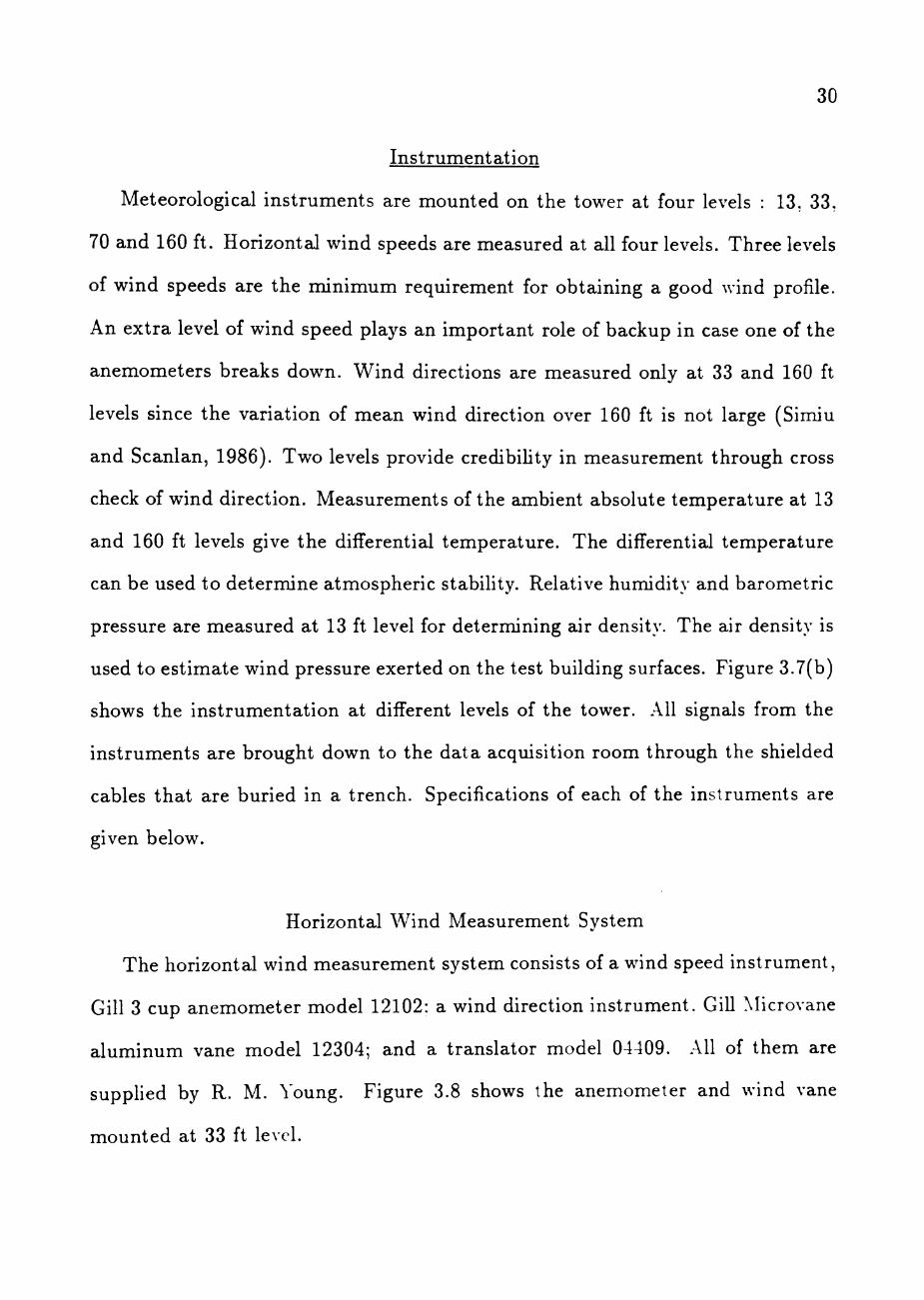
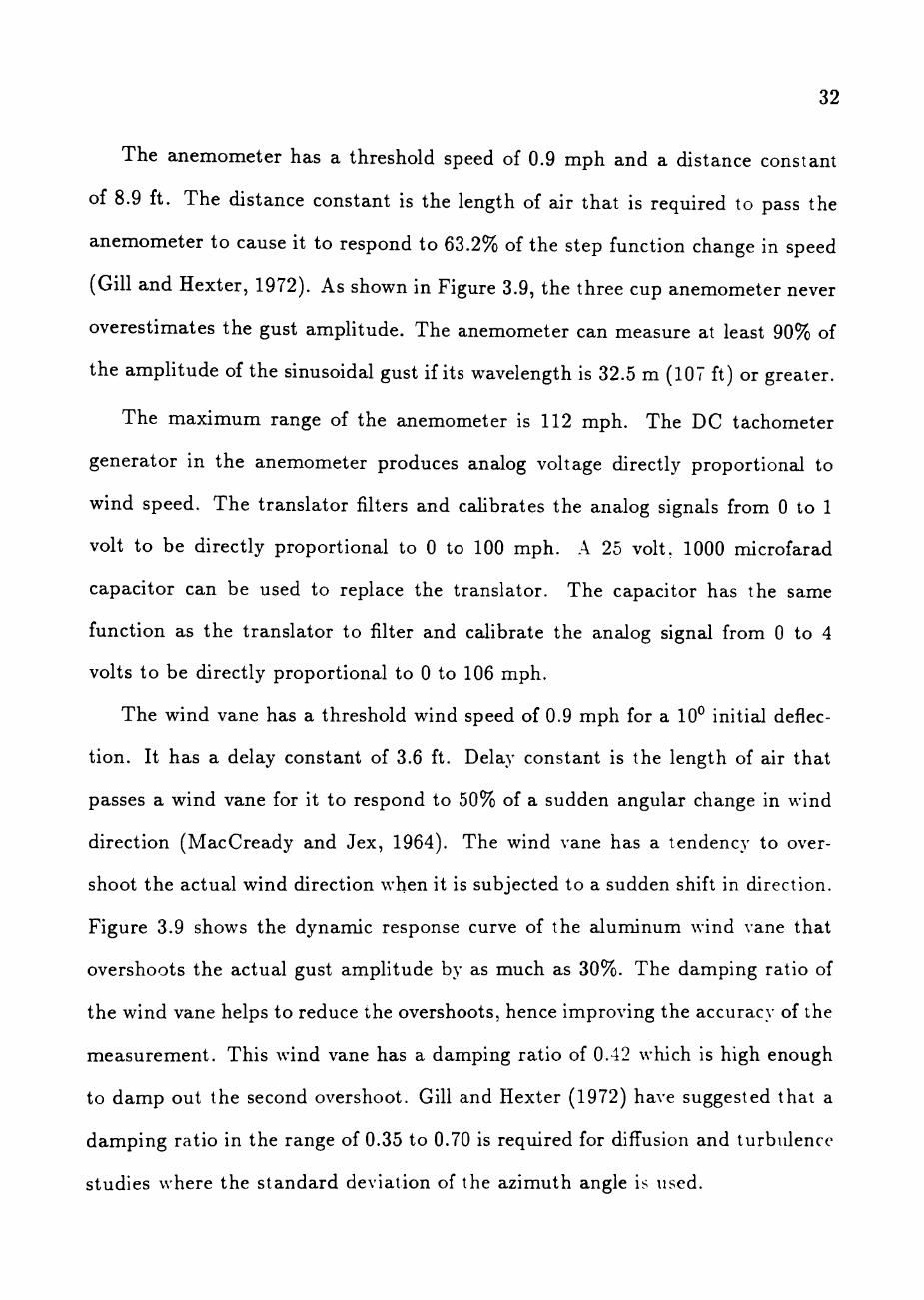
Instrumentation

Meteorological instruments are mounted on the tower at four levels : 13, 33,

70 and 160 ft. Horizontal wind speeds are measured at all four levels. Three levels

of wind speeds are the minimum requirement for obtaining a good wind profile.

An extra level of wind speed plays an important role of backup in case one of the

anemometers breaks down. Wind directions are measured only at 33 and 160 ft

levels since the variation of mean wind direction over 160 ft is not large (Simiu

and Scanlan, 1986). Two levels provide credibifity in measurement through cross

check of wind direction. Measurements of the ambient absolute temperature at 13

and 160 ft levels give the differential temperature. The differential temperature

can be used to determine atmospheric stability. Relative humidity and barometric

pressure are measured at 13 ft level for determining air density. The air density is

used to estimate wind pressure exerted on the test building surfaces. Figure 3.7(b)

shows the instrumentation at different levels of the tower. All signals from the

instruments are brought down to the data acquisition room through the shielded

cables that are buried in a trench. Specifications of each of the instruments are

given below.

Horizontal Wind Measurement System

The horizontal wind measurement system consists of a wind speed instrument,

Gill 3 cup anemometer model 12102: a wind direction instrument. Gill Microvane

aluminum vane model 12304; and a translator model 04409. All of them are

supphed by R. M. Young. Figure 3.8 shows the anemometer and wind vane

mounted at 33 ft level.

31

Figure 3.8 Anemometer and Wind Vane at 33 ft Level

32

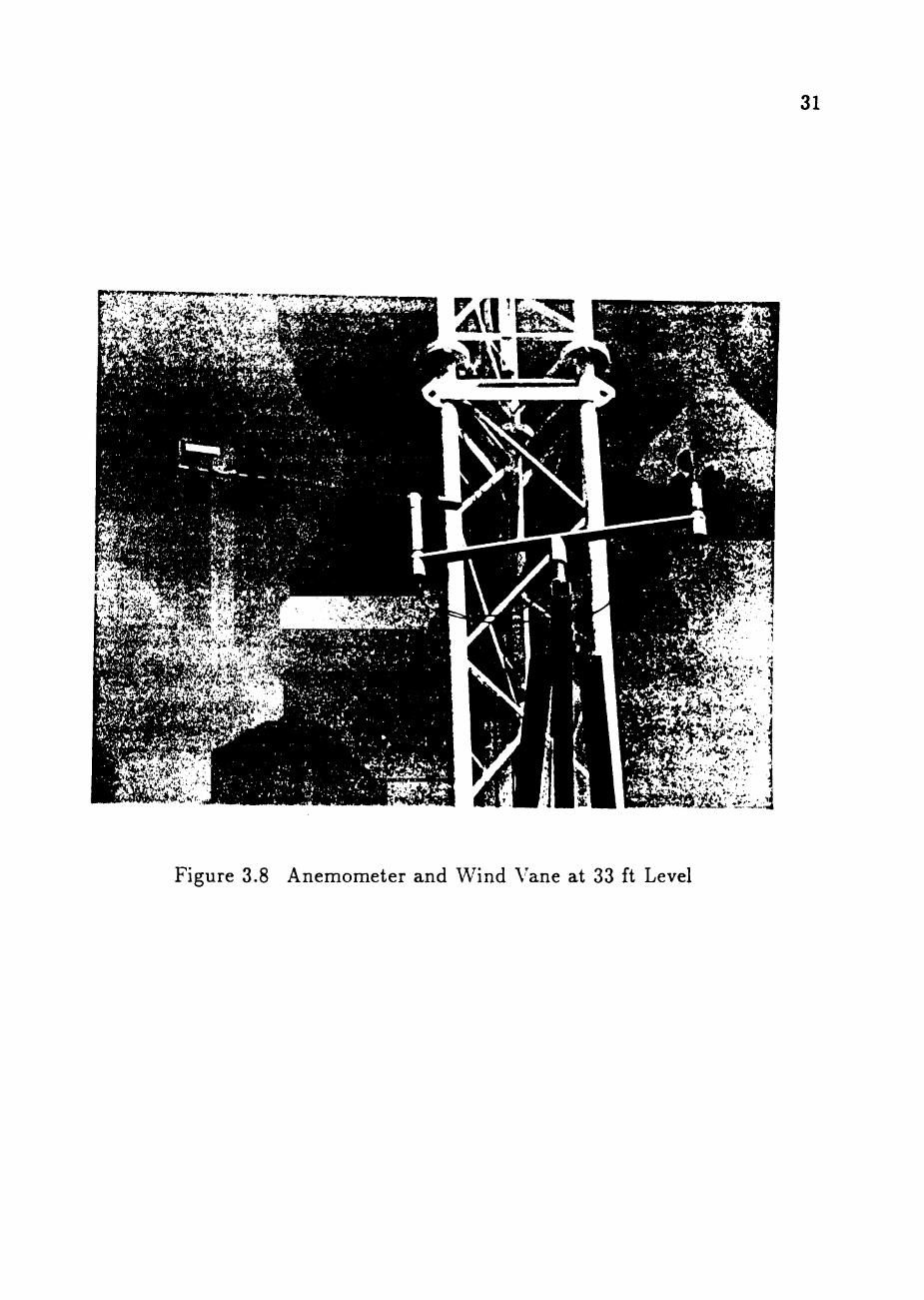
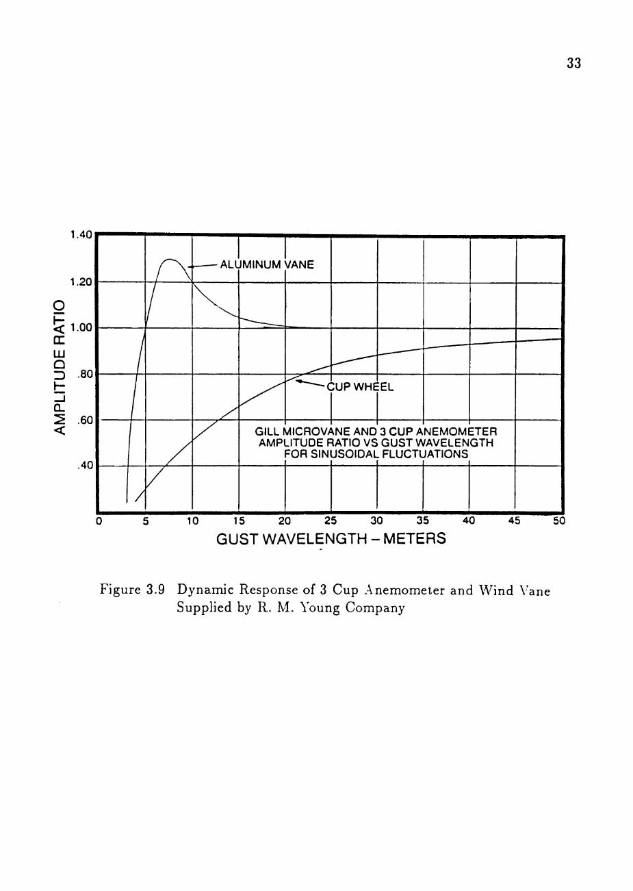
The anemometer has a threshold speed of 0.9 mph and a distance constant

of 8.9 ft. The distance constant is the length of air that is required to pass the

anemometer to cause it to respond to 63.2% of the step function change in speed

(Gill and Hexter, 1972). As shown in Figure 3.9, the three cup anemometer never

overestimates the gust ampHtude. The anemometer can measure at least 90% of

the ampHtude of the sinusoidal gust if its wavelength is 32.5 m (107 ft) or greater.

The maximum range of the anemometer is 112 mph. The DC tachometer

generator in the anemometer produces analog voltage directly proportional to

wind speed. The translator filters and calibrates the analog signals from 0 to 1

volt to be directly proportional to 0 to 100 mph. A 25 volt. 1000 microfarad

capacitor can be used to replace the translator. The capacitor has the same

function as the translator to filter and calibrate the analog signal from 0 to 4

volts to be directly proportional to 0 to 106 mph.

The wind vane has a threshold wind speed of 0.9 mph for a 10° initial deflec­

tion. It has a delay constant of 3.6 ft. Delay constant is the length of air that

passes a wind vane for it to respond to 50% of a sudden angular change in wind

direction (MacCready and Jex, 1964). The wind vane has a tendency to over­

shoot the actual wind direction when it is subjected to a sudden shift in direction.

Figure 3.9 shows the dynamic response curve of the aluminum wind vane that

overshoots the actual gust amplitude by as much as 30%. The damping ratio of

the wind vane helps to reduce the overshoots, hence improving the accuracy of the

measurement. This wind vane has a damping ratio of 0.42 which is high enough

to damp out the second overshoot. Gill and Hexter (1972) have suggested that a

damping ratio in the range of 0.35 to 0.70 is required for diffusion and turbulence

studies where the standard deviation of the azimuth angle is used.

33

1.40

1.20

!< 1.00 DC LU Q D

IE <

.80

.60

.40

/

GILL MICROVANE AND 3 CUP ANEMOMETER AMPLITUDE RATIO VS GUST WAVELENGTH

FOR SINUSOIDAL FLUCTUATIONS

10 15 20 25 30 35 40

GUST WAVELENGTH - METERS 45 50

Figure 3.9 Dynamic Response of 3 Cup Anemometer and Wind Vane Supplied by R. M. Young Company

34

The wind direction signal is from a precision linear conductive plastic type

potentiometer which provides an analog output signal of 0 to 1 volt directly

proportional to the angle of 0° to 360°. The potentiometer requires a constant

excitation voltage suppHed by a translator. The operating range of the wind vane

is from the angle of 0° to 355°; the potentiometer has a dead band of 5°.

Because the measurements from north are important for this project, the 0°

of the wind vane is aHgned to the field azimuth of 120°. This azimuth is in Hne

with the boom. Thus the dead band of the instrument is located in the directions

where wind data are not usable in this project.

Temperature Measurement System

The temperature measurement system, supplied by Teledyne Geotech, consists

of a platinum temperature sensor, a wind aspirated thermal radiation shield and

a processor. Two different temperature sensors are used. For temperature mea­

surement at 13 ft level, a relative humidity/platinum temperature sensor model

RH-200 (capable of measuring both relative humidity and temperature on one

probe) housed in a wind aspirated thermal shield model WAS-300 is used. A

calibrated platinum temperature sensor model T-200 housed in a wind aspirated

thermal radiation shield model WAS-100 is used to measure temperature at 160

ft level. Signals from each sensor is processed by a temperature processor model

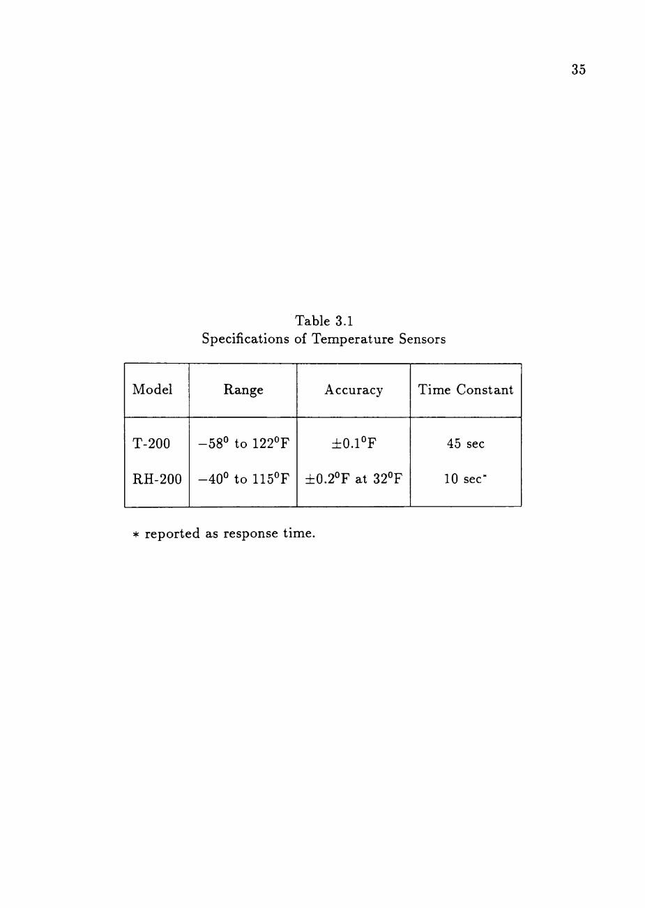
10.32. Table 3.1 shows the specifications of the temperature sensors.

Both temperature sensors are platinum resistance temperature sensors. This

resistance sensor measures the electrical resistance of the platinum which increases

non-linearly with increase in ambient absolute temperature. The non-linear signal

is linearized by the temperature processor.

35

Table 3.1 Specifications of Temperature Sensors

Model

T-200

RH-200

Range

-58° to 122°F

-40° to 115°F

Accuracy

±0.1°F

±0.2°F at 32°F

Time Constant

45 sec

10 sec"

* reported as response time.

36

The temperature processor regulates the excitation voltage to the sensor. It

also filters, conditions, amplifies and linearizes the non-Hnear signals so that 0

to 5 volts is directly proportional to -58° to 122°F. The processor's accuracy is

±0.1°F for operating temperature of 77° ~ 9°F. The accuracy decreases to i0 .2°F

outside the operating range.

The wind aspirated thermal radiation shield acts as an effective shield to

temperature sensor against the effects of solar and terrestrial radiation. Direct

exposure of the sensor to the radiation will cause the sensor to give incorrect

ambient absolute temperature.

Relative Humidity Measurement System

The relative humidity measurement system, supplied by Teledyne Geotech. is

a combination of a relative humidity/platinum temperature sensor model RH-200

housed in a wind aspirated thermal radiation shield model WAS-300 and a relative

huniidity processor model 10.41/33. The RH-200 sensor and WAS-300 shield are

also used to measure temperature at 13 ft level as mentioned previously.

The relative humidity sensor has a measuring range of 0 to 100% relative

humidity and a response time of 5 seconds. The accuracy of the sensor is ±2%

from 0 to 80% and ± 3 % above 80% relative humidity.

The relative humidity processor regulates the excitation voltage to the sensor.

The signal is filtered, conditioned and amphfied to a gain of 50 . \'oltage signal

of 0 to 5 volts is directly proportional to 0 to 100% relative humidity.

Barometric Pressure Measurement System

The barometric pressure measurement system consists of a barometric pressure

sensor model BP-lOO and a barometric pressure processor model 10.22/61. Both

the sensor and the processor are suppHed by Teledyne Geotech.

The BP-lOO has a range of 24.3 to 31.5 in Hg which covers ah normal range

of absolute barometric pressure in the Lubbock area. The average absolute baro­

metric pressure in Lubbock is 27 in Hg. The BP-lOO has a resolution of 0.15% of

the range span which is 0.01 in Hg.

The processor regulates excitation voltage to the sensor. It also filters and

conditions the output signal. No amplification of signal is involved since the

output signal of 0 to 5 volts is directly proportional to 24.3 to 31.5 in Hg.

Data Acquisition System

The data acquisition system samples the instrument signals in term of voltage

and converts the analog signals to digital signals. The digitized data are stored

in appropriate form for future analysis. The data acquisition is controlled by an

IBM PC XT computer housed in the data acquisition room.

Analog instrument signals are converted to digital form using a MetraByte

DAS-8 analog/digital convertor. This DAS-8 has the capability of converting

signals at a rate of 4000 Hz through eight input channels. Each input channel

is expanded to sixteen channels using MetraByte Universal Expansion Interface

board, EXP-16. The EXP-16 is an expansion multiplexer and amplifier system

that provides signal amplification, filtering and conditioning. With the use of

eight EXP-16, the system can be expanded to a maximum of 128 channels. Four

EXP-16 are used to provide 64 channels of data for this project.

38

Software acquired from Laboratory Technologies Corporation, LABTECH

NOTEBOOK, is the key to the data acquisition system. LABTECH NOTE­

BOOK is a user-friendly software that aHow different channels to be set up with

different characteristics. It also allows real time display of the incoming data

which is very helpful for caHbration of the instrumentation.

The software can be set to trigger automatically when the wind speed reaches

a preset threshold level. Once triggered, the system is programmed to sample

data at a rate of 10 Hz for all meteorological channels except relative humidity

and barometric pressure channels which are sampled at 1 Hz. for a continuous

period of 15 minutes. After completing one record, the one minute average wind

speed is checked and another recording begins if the wind speed is still above

the threshold level. The records collected for this study are triggered manually.

Automatic triggering system is still being setup at this writing.

Once the data are sampled and digitized, they are streamed directly to a 20

megabyte BernoulH removable cartridge drive by the LABTECH NOTEBOOK.

This streaming ehminates the limitation imposed by the computer memory to the

duration of each record. Each removable cartridge can store a few hours of data.

The removable cartridge is brought back to Texas Tech University campus

and uploaded to the DEC \ AX-8650 computer. The uploading process is made

possible by the MS-Kermit software which is controlled by an IBM Personal Sys­

tem/2 model 60 computer. All uploaded data are stored in magnetic tapes for

future analysis.

CHAPTER IV

CALIBRATION OF METEOROLOGICAL

INSTRUMENTS

All the meteorological instruments are purchased off the shelf from two com­

panies, R. M. Young and Teledyne Geotech. They have been checked and certified

by the manufacturers to be in good working condition. However, it is the respon­

sibility of this field experiment research team to verify the accuracy and field

applicability before using them in the field.

Meteorological instrument records the meteorological parameters and gives out

the output in terms of electrical signal. A controlled meteorological parameter

such as wind speed in wind tunnel, can be measured simultaneously by the new

meteorological instrument and at least one other dependable instrument. The

results of both instruments are compared to verify the new instrument.

Anemometers, wind vanes, and temperature, relative humidity and barometric

pressure sensors are tested in the laboratory and in the field wherever possible.

Effect of the cable length on the electrical signal is also checked in the laboratory.

Anemometer

The accuracy of the anemometers is checked in the 3x4 ft wind tunnel located

in the mechanical engineering department. The anemometer is mounted on a

tripod and is placed in the center of the cross-section of the wind tunnel. A pitot-

static tube is placed at the same height but 10 inches beside the anemometer. This

arrangement assures both instruments experience the wind flows with minimum

interference of the wind tunnel's walls.

39

40

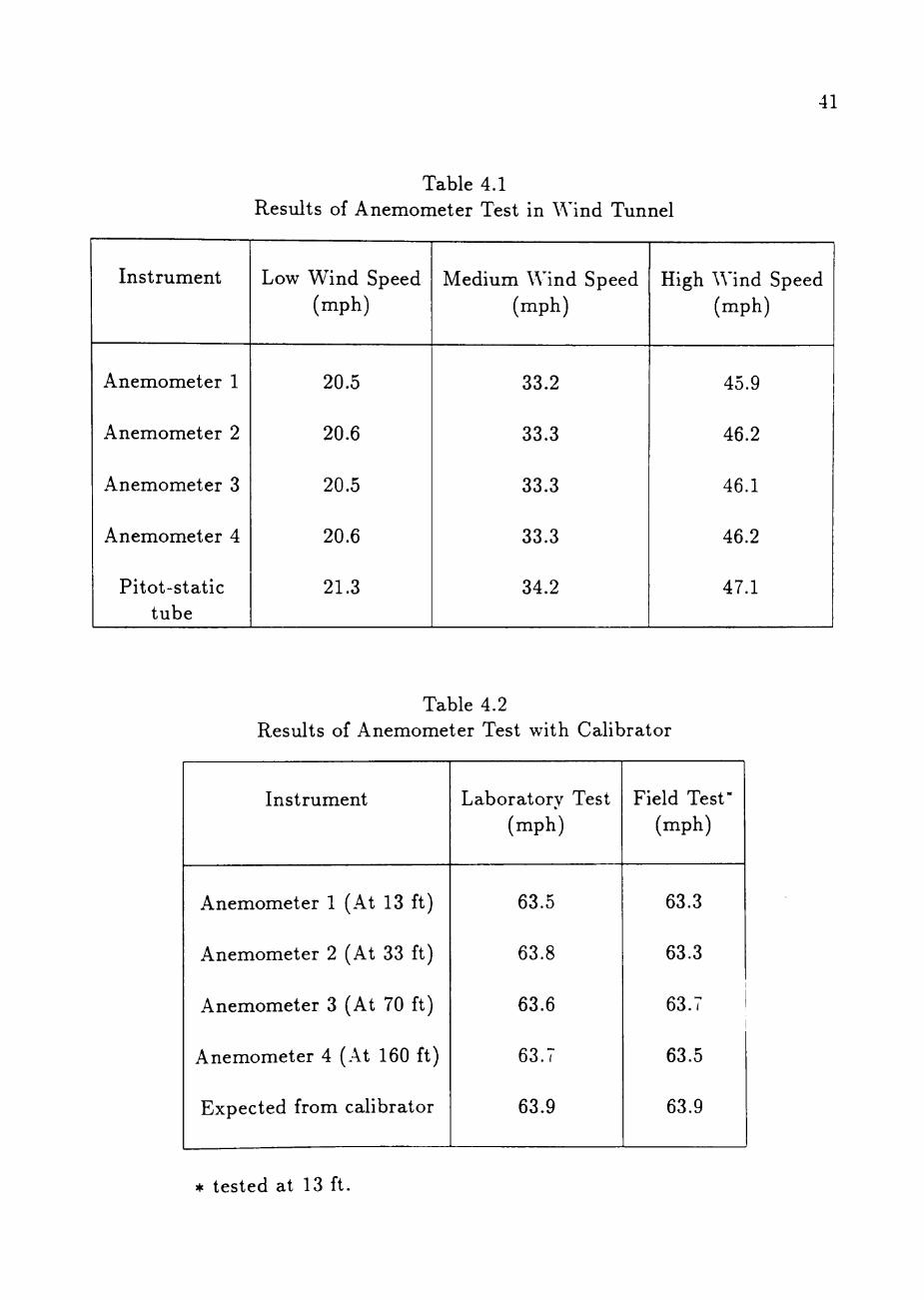
Three different wind tunnel speeds that are representative of the expected wind

speed in the field are used to test the anemometers. The pitot-static tube provides

the reference wind speed in the wind tunnel. Wind speed of the anemometer is

recorded at 10 Hz by the same data acquisition system that wih be used in the

field. Table 4.1 shows the mean wind speeds recorded by four anemometers at

three different wind speeds. The reference wind speeds recorded by the pitot-stalic

tube are slightly higher than the mean wind speeds recorded by the anemome­

ters. The difference is approximately 3%. The difference is considered acceptable

because the mean wind speeds recorded by the four anemometers are very close

to each other. The variation among the anemometers in the recorded speeds is

within the range of 0.1 to 0.3 mph which corresponds to less than 1% of the mean

speed.

Electrical signal of the anemometer can be checked for accuracy using a com­

mercial calibrator. The calibrator is a motor with constant speed of 1800 rpm.

A rubber tubing connects the shaft of the anemometer to the calibrator. The

anemometer cup has to be removed when using calibrator. Rotation of the

anemometer shaft at 1800 rpm corresponds to wind speed of 63.9 mph. All the

ariemometers have been tested with the calibrator in the laboratory and in the

field. Anemometer mounted at 13 ft level can be tested in the field. Anemome­

ters for the 33, 70 and 160 ft levels are brought down and mounted at 13 ft

for calibrator test. Results of the caHbrator tests are shown in Table 4.2. Both

the laboratory and the field test results indicate that the electrical signal of the

anemometers correspond to slightly less than the expected wind speed. The dif­

ference however is small, less than 1%.

41

Table 4.1 Results of Anemometer Test in Wind Tunnel

Instrument

Anemometer 1

Anemometer 2

Anemometer 3

Anemometer 4

Pitot-static tube

Low Wind Speed (mph)

20.5

20.6

20.5

20.6

21.3

Medium Wind Speed (mph)

33.2

33.3

33.3

33.3

34.2

High Wind Speed (mph)

45.9

46.2

46.1

46.2

47.1

Table 4.2 Results of Anemometer Test with Calibrator

Instrument

Anemometer 1 (At 13 ft)

Anemometer 2 (At 33 ft)

Anemometer 3 (At 70 ft)

Anemometer 4 (At 160 ft)

Expected from calibrator

Laboratory Test (mph)

63.5

63.8

63.6

63.7

63.9

Field Test-(mph)

63.3

63.3

63.7

63.5

63.9

* tested at 13 ft,

42

The caHbrator test results show noticeable fluctuations in the electrical signal.

The fluctuations are found to be equivalent to the turbulence intensity of 1.5% at

mean wind speed of 63.9 mph. This fluctuation in signal is probably due to noise

of the DC generator in the anemometer.

Both the wind tunnel and caHbrator tests of the anemometers show that the

anemometers are in good working condition. The accuracy of the anemometers

is satisfactory.

W ind Vane

The balance, range and accuracy of the wind vanes have been tested in the

laboratory before mounting them on the tower. The vane balance is tested easily

by laying the vane on its side on a table. The vane shaft which has a counterweight

at one end and a fin at the other end, is free to rotate. A balanced vane would

let the shaft remain horizontaUy and will not have tendency to change position.

Both the wind vane instruments are found to be balanced.

The range and accuracy of the wind vane instruments are tested by connecting

the wind vane with the signal conditioning translator to the field data acquisition

system. To check the operating range, the wind vane is rotated through a complete

revolution. Data collected during the rotation show that the operating range is

from 0° to 355°. Angle in the range of 356° to 360° is dead band (zero signal).

The accuracy of the wind vane is tested by aligning the wind vane with known

angles. The known angles are sketched on a transparency with the angles of 0°,

45°, 90°, 135°, 180°, 225°, 270° and 315°. The 0° angle on the transparency is

aligned with the 0° angle of the wind vane. Once the 0° angle is estabHshed, the

wind vane is rotated and aligned with the next angle on the transparency. The

43

angle on the visual display is recorded. This process is repeated for aU the angles

on the transparency. The visual display results show that the deviations of the

wind vane angles are within ±4° of the angles on the transparency. The difference

can be due to the resolution of the visual display and the difficulty in aligning

the wind vane with the transparency. Since the electrical signal from the vane is

found to be Hnear from 0° to 355°, the wind vane is considered to provide desired

accuracy.

Temperature Sensor

The accuracy of the two temperature sensors, T-200 and RH-200 are checked

against a mercurial thermometer and a Weathertronics model 4480 temperature

sensor. The mercurial thermometer and the Weathertronics sensor have the ac­

curacy of ±1°F and ±0.1°F respectively.

Temperature readings from T-200 and RH-200 sensors are recorded by the field

data acquisition system at a sampling rate of 10 Hz. The output signal of the

Weathertronics sensor is indicated by a digital voltmeter and recorded by hand.

Temperature of the mercurial thermometer is monitored visually and recorded

immediately after sensors' temperature readings are recorded.

To test the upper range of the sensors, all three sensors and the thermometer

are placed in an oven. Data is collected only when the sensors reach a steady state

temperature. The sensors are also tested at room temperature, near freezing and

below freezing temperatures. It is observed that the sensors take about 20 to 30

minutes to reach a steady state temperature of the environment.

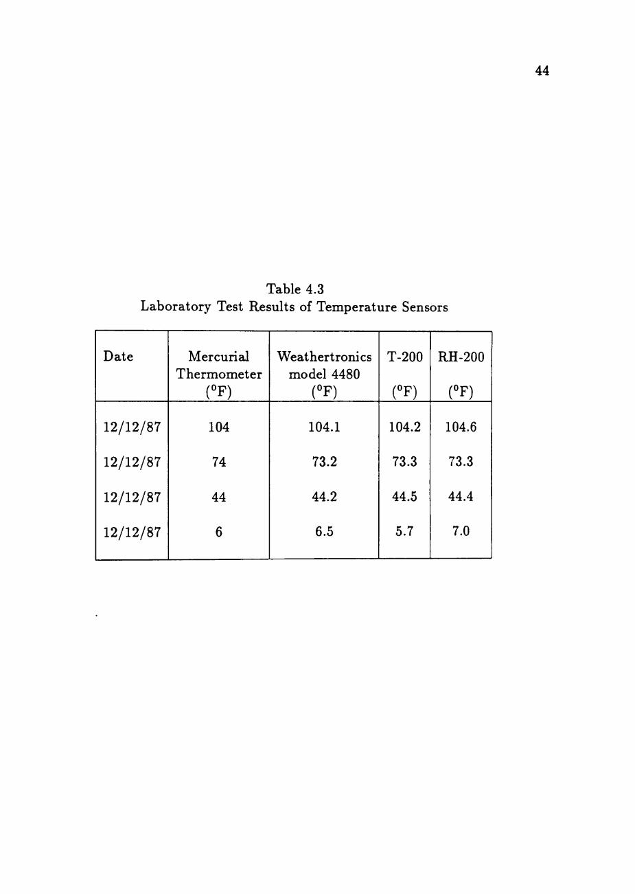
Results of the laboratory tests are tabulated in Table 4.3. Temperature read­

ings at 104°, 74° and 44°F recorded by the sensors and thermometer are very

44

Table 4.3 Laboratory Test Results of Temperature Sensors

Date

12/12/87

12/12/87

12/12/87

12/12/87

Mercurial Thermometer

(°F)

104

74

44

6

Weathertronics model 4480

(°F)

104.1

73.2

44.2

6.5

T-200

(°F)

104.2

73.3

44.5

5.7

RH-200

(°F)

104.6

73.3

44.4

7.0

45

close. The difference between the T-200 and RH-200 readings are within the

sensor accuracy and possible temperature processor error. Results of the temper­

ature readings at 7°F show some variation. The reason of this variation at low

temperature is not known. However, the variation in temperature recordings at

below freezing temperature of 7°F is not critical in this project because strong

winds are not likely to occur during this low a temperature.

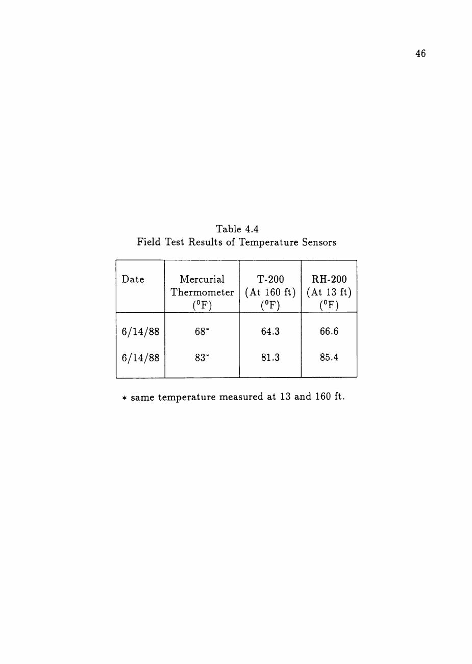
Field test of the T-200 and RH-200 sensors are also carried out with the same

mercurial thermometer used in the laboratory test. The atmospheric stabihty

condition on the test day is assumed to be stable since there was almost no wind.

It was expected that the temperature difference between 13 and 160 ft levels

would be less than the dry adiabatic rate, that is less that 0.8°F. The recordings

are taken after the thermometer is held in the shade for 10 minutes. The results

of the field tests are tabulated in Table 4.4. The temperature readings of the

mercurial thermometer at 13 and 160 ft levels are the same. The reason is the

inability of thermometer to measure the sHght temperature difference between

the two levels. The thermometer readings are not close to the readings of the

sensors. Also, there is a 2° and 4°F difference between the two sensors' readings.

The difference is much greater than the expected temperature of less than 0.8°F.

This difference in recordings by the sensors suggest that the instruments are not

usable to assess atmospheric stabihty. Additional field calibration and checking

are necessary before using the temperature readings to assess stability of the

atmosphere.

46

Table 4.4 Field Test Results of Temperature Sensors

Date

6/14/88

6/14/88

Mercurial Thermometer

(°F)

68-

83-

T-200 (At 160 ft)

(°F)

64.3

81.3

RH-200 (At 13 ft)

(°F)

66.6

85.4

* same temperature measured at 13 and 160 ft.

47

Relative Humidity Sensor

The laboratory test of the relative humidity sensor, RH-200 is to check the

range of the sensor. The RH-200 sensor is placed in the humidity room which

is believed to have close to 100% relative humidity (RH). The output signal is

indicated by a voltmeter and recorded by hand. The laboratory RH during the

test is 23%. Once the sensor is placed in the humidity room, an increase of RH is

noticed. The final humidity room RH is 96%. It is therefore concluded that the

operating range of the RH-200 sensor is at least 23% to 96% RH.

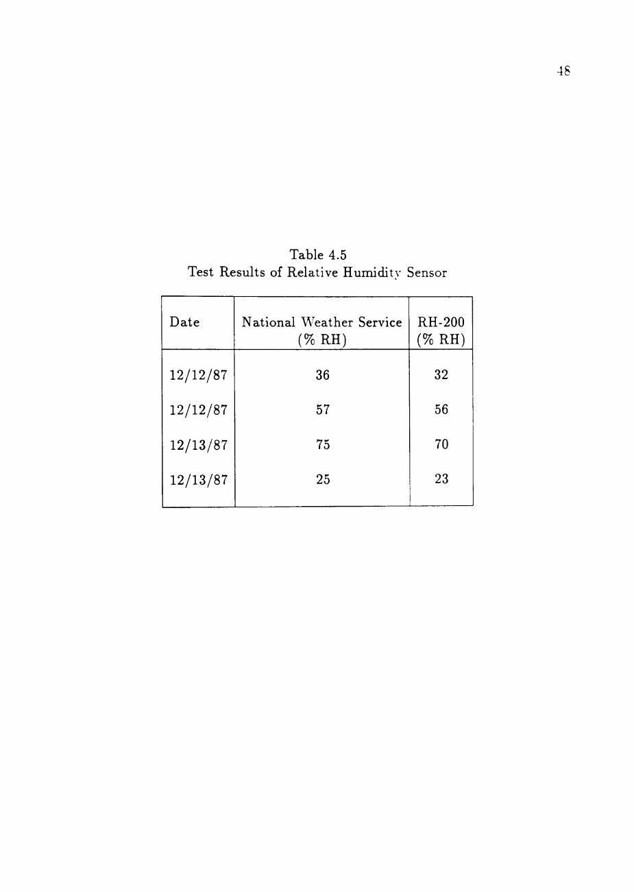
Another RH sensor is not available to check the accuracy RH-200 sensor in the

laboratory. One way of checking the accuracy of the sensor in the field is to com­

pare RH measured by RH-200 with the RH measured by the National Weather

Service station at the Lubbock International Airport, about 7 miles from the test

site. The RH-200 sensor is mounted on the tower at 13 ft level. The output

is indicated by a digital voltmeter and recorded by hand. The RH reading is

recorded at the beginning of the hour when the National Weather Service up­

dates weather information. Table 4.5 shows the field test results. The maximum

difference between RH-200 and National Weather Service measurements is 5%

RH. A difference of 5% in RH is considered acceptable because it has negligible

effect on the density of air.

Barometric Pressure Sensor

The barometric pressure sensor, BP-lOO, is checked ageiinst a barometer pres­

sure sensor, Weathertronics model 71101 and a mercurid barometer. The mercu­

rial barometer is located in mechanical engineering laboratory, which is about 200

ft away from the laboratory test location. Signals from the BP-lOO is recorded

48

Table 4.5 Test Results of Relative Humiditv Sensor

Date

12/12/87

12/12/87

12/13/87

12/13/87

National Weather Service (% RH)

36

57

75

25

RH-200 (% RH)

32

56

70

23

49

by the field data acquisition system at a sampUng rate of 1 Hz. A voltmeter is

used to indicate the signal from the Weathertronics barometric pressure sensor.

The mercurial barometer reading is recorded after the completion of the data

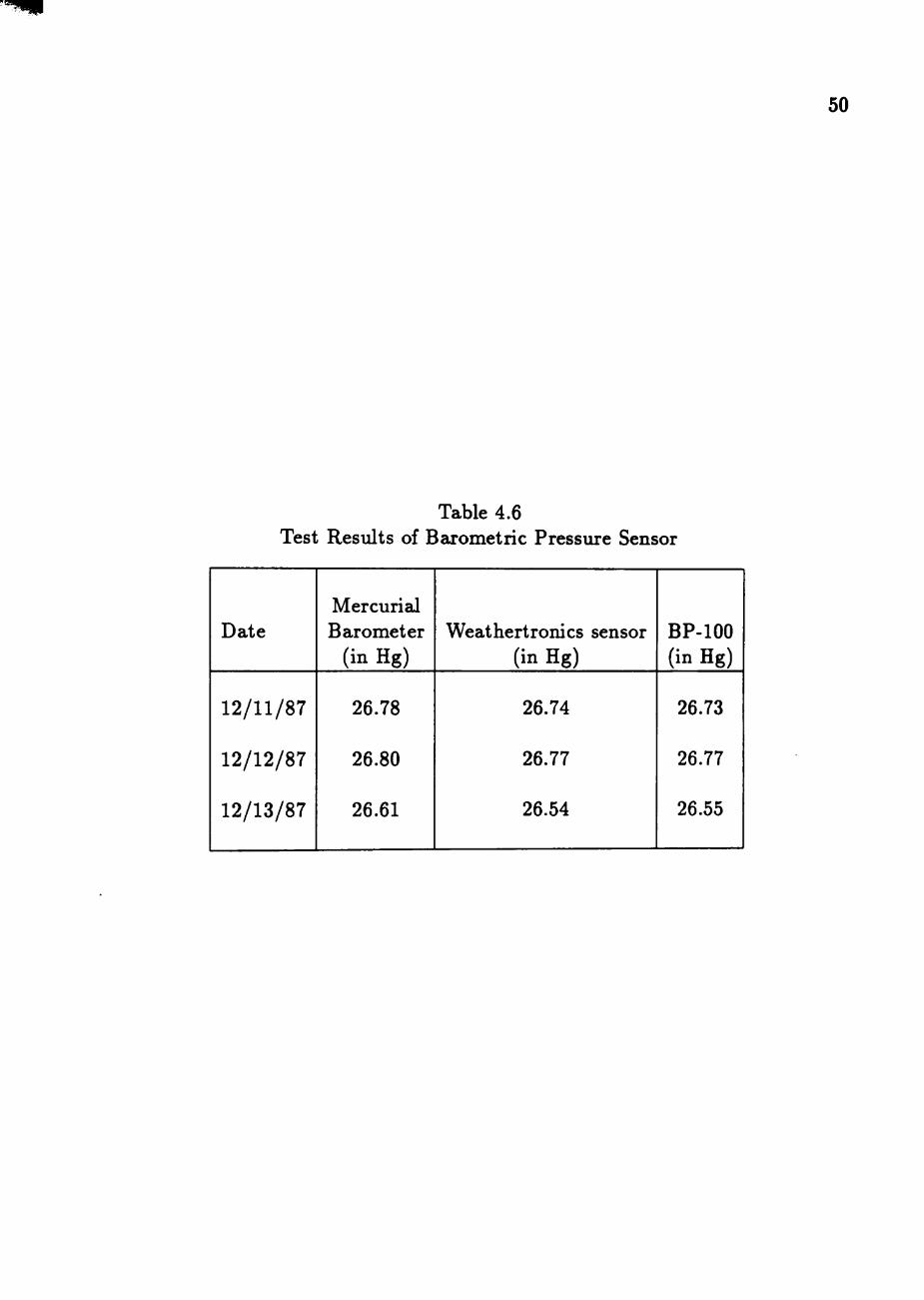
collection of two sensors. Results tabulated in Table 4.6 show that the difference

between BP-lOO and Weathertronics sensor readings is 0.01 in Hg. The mercurial

barometer readings are 0.04 to 0.07 in Hg higher than the sensors' readings. The

close results of the BP-lOO and Weathertronics sensor readings give the assurance

that the BP-lOO sensor is in good working condition.

Cable Effect

Two different cables are used for the tower instruments. Signals from wind in­

struments are carried by multi-conductor cables. Shielded multi-conductor cables

are used for carrying signals from temperature, relative humidity and barometric

pressure sensors. The conductors for both cables are 20 gage. Effect of the cable

length on electrical signal is tested for both cables.

The length of the cable reduces the electrical output signals from the instru­

ments. The effect can be checked by supplying a known input voltage to one end

of the cable and measuring the output voltage at the other end of the cable. The

difference between the input and output voltage is the voltage reduction caused

by the resistance of the cable. Two different lengths of cable, 50 and 375 ft are

used in the tests. The 375 ft is the length of the cable for instruments located at

160 ft level of the tower. The test results indicate that the input voltage is equal

to the output voltage with an accuracy of 0.001 volt. This voltage is equivalent

to wind speed of 0.1 mph, wind direction angle of 0.4° and temperature of 0.04°F.

Thus, the length effect of the cable is within the acceptable tolerance.

50

Table 4.6 Test Residts of Barometric Pressure Sensor

Date

12/11/87

12/12/87

12/13/87

Mercurial Barometer

(in Hg)

26.78

26.80

26.61

Weathertronics sensor (in Hg)

26.74

26.77

26.54

BP-lOO (in Hg)

26.73

26.77

26.55

CHAPTER V

ANALYSIS OF FIELD DATA

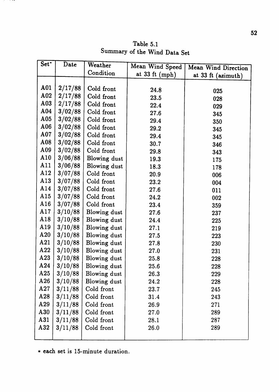
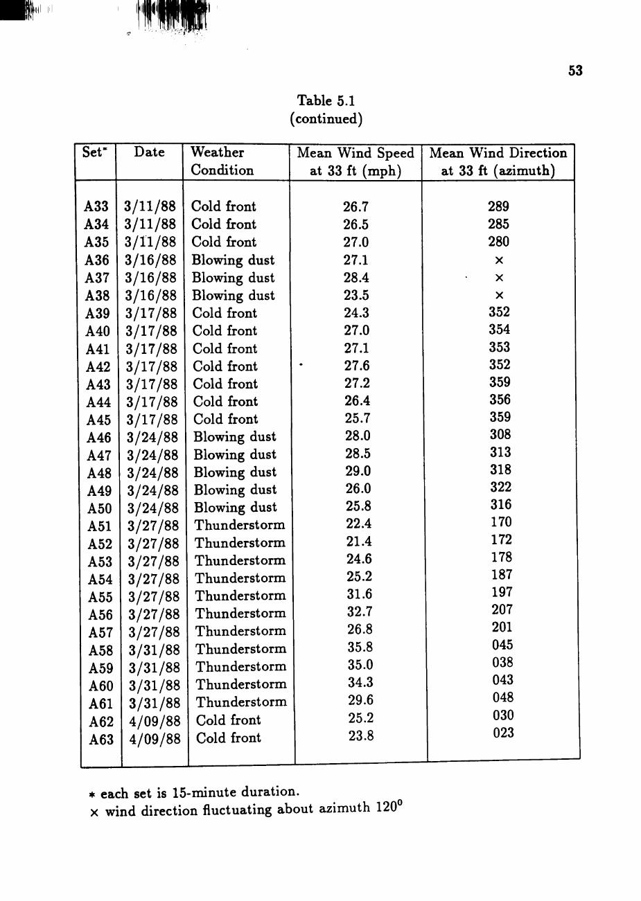
One of the objectives of this study is to assess the wind parameters of Texas

Tech University field site from field wind data. A total of 63 sets of field wind data

are collected during the period from February to April, 1988. Different weather

conditions are encountered during this data collection period. The weather con­

ditions include cold front, thunderstorm and gusty blowing dust. Table 5.1 shows

the summary of all the data sets. Each set of data consists of four wind speed

records collected at 13, 33, 70 and 160 ft levels; two wind direction records col­

lected at 33 and 160 ft levels; and two temperature records measured at 13 and

160 ft levels. Each record is collected at 10 Hz over a continuous period of 15

minutes. The first 24 sets of wind speed data are collected with translators for

33 and 160 ft level anemometers, and the other two records are collected with

capacitors. The rest of the wind speed sets are collected with four capacitors.

A statistical analysis of the data is presented here. Time histories of the

wind records are plotted for visual inspection. Descriptive statistics of the wind

records are also calculated for validation of data. Stationarity of the wind speed

and wind direction records are checked. Neutral atmospheric stability condition

during the time of data collection is assumed to exist when the mean wind speed

at 33 ft level exceeds 20 mph. Only stationary records that are in neutral stability

condition are used for analysis. Analysis of the wind records include wind profile

parameters, turbulence intensity and longitudinal integral scale of turbulence.

The wind profile parameters are used to characterize the field terrain. Results of

the analysis are presented.

51

52

Table 5.1 Summary of the Wind Data Set

Set-

AOl A02 A03 A04 A05 A06 A07 A08 A09 AlO Al l A12 A13 A14 A15 A16 A17 A18 A19 A20 A21 A22 A23 A24 A25 A26 A27 A28 A29 A30 A31 A32

Date

2/17/88 2/17/88 2/17/88 3/02/88 3/02/88 3/02/88 3/02/88 3/02/88 3/02/88 3/06/88 3/06/88 3/07/88 3/07/88 3/07/88 3/07/88 3/07/88 3/10/88 3/10/88 3/10/88 3/10/88 3/10/88 3/10/88 3/10/88 3/10/88 3/10/88 3/10/88 3/11/88 3/11/88 3/11/88 3/11/88 3/11/88 3/11/88

Weather Condition

Cold front Cold front Cold front Cold front Cold front Cold front Cold front Cold front Cold front Blowing dust Blowing dust Cold front Cold front Cold front Cold front Cold front Blowing dust Blowing dust Blowing dust Blowing dust Blowing dust Blowing dust Blowing dust Blowing dust Blowing dust Blowing dust Cold front Cold front Cold front Cold front Cold front Cold front

Mean Wind Speed at 33 ft (mph)

24.8 23.5 22.4 27.6 29.4 29.2 29.4 30.7 29.8 19.3 18.3 20.9 23.2 27.6 24.2 23.4 27.6 24.4 27.1 27.5 27.8 27.0 25.8 25.6 26.3 24.2 23.7 31.4 26.9 27.0 28.1 26.0

Mean Wind Direction at 33 ft (azimuth)

025 028 029 345 350 345 345 346 343 175 178 006 004 Oil 002 359 237 225 219 223 230 231 228 228 229 228 245 243 271 289 287 289

* each set is 15-minute duration.

53

(

Set"

A33 A34 A35 A36 A37 A38 A39 A40 A41 A42 A43 A44 A45 A46 A47 A48 A49 A50 A51 A52 A53 A54 A55 A56 A57 A58 A59 A60 A61 A62 A63

Date

3/11/88 3/11/88 3/11/88 3/16/88 3/16/88 3/16/88 3/17/88 3/17/88 3/17/88 3/17/88 3/17/88 3/17/88 3/17/88 3/24/88 3/24/88 3/24/88 3/24/88 3/24/88 3/27/88 3/27/88 3/27/88 3/27/88 3/27/88 3/27/88 3/27/88 3/31/88 3/31/88 3/31/88 3/31/88 4/09/88 4/09/88

Weather Condition

Cold front Cold front Cold front Blowing dust Blowing dust Blowing dust Cold front Cold front Cold front Cold front Cold front Cold front Cold front Blowing dust Blowing dust Blowing dust Blowing dust Blowing dust Thunderstorm Thunderstorm Thunderstorm Thunderstorm Thunderstorm Thunderstorm Thunderstorm Thunderstorm Thunderstorm Thunderstorm Thunderstorm Cold front Cold front

Table 5.1 continued)

Mean Wind Speed at 33 ft (mph)

26.7 26.5 27.0 27.1 28.4 23.5 24.3 27.0 27.1 27.6 27.2 26.4 25.7 28.0 28.5 29.0 26.0 25.8 22.4 21.4 24.6 25.2 31.6 32.7 26.8 35.8 35.0 34.3 29.6 25.2 23.8

Mean Wind Direction at 33 ft (azimuth)

289 285 280

X

X

X

352 354 353 352 359 356 359 308 313 318 322 316 170 172 178 187 197 207 201 045 038 043 048 030 023

* each set is IS-minute duration. X wind direction fluctuating about azimuth 120

54

Time History

The first step in time series analysis is to plot the time history of the record.

A time history is a plot of observed values versus time. It is useful in detecting

discontinuities, trends and patterns.

Time histories of all the wind speed and wind direction records are plotted

by averaging over every 10 points (1 second average). Descriptive statistics such

as mean, root mean square, maximum and minimum values are also calculated

during the plots. The mean and root mean square lines are also plotted on the

time history for the ease of visual inspection.

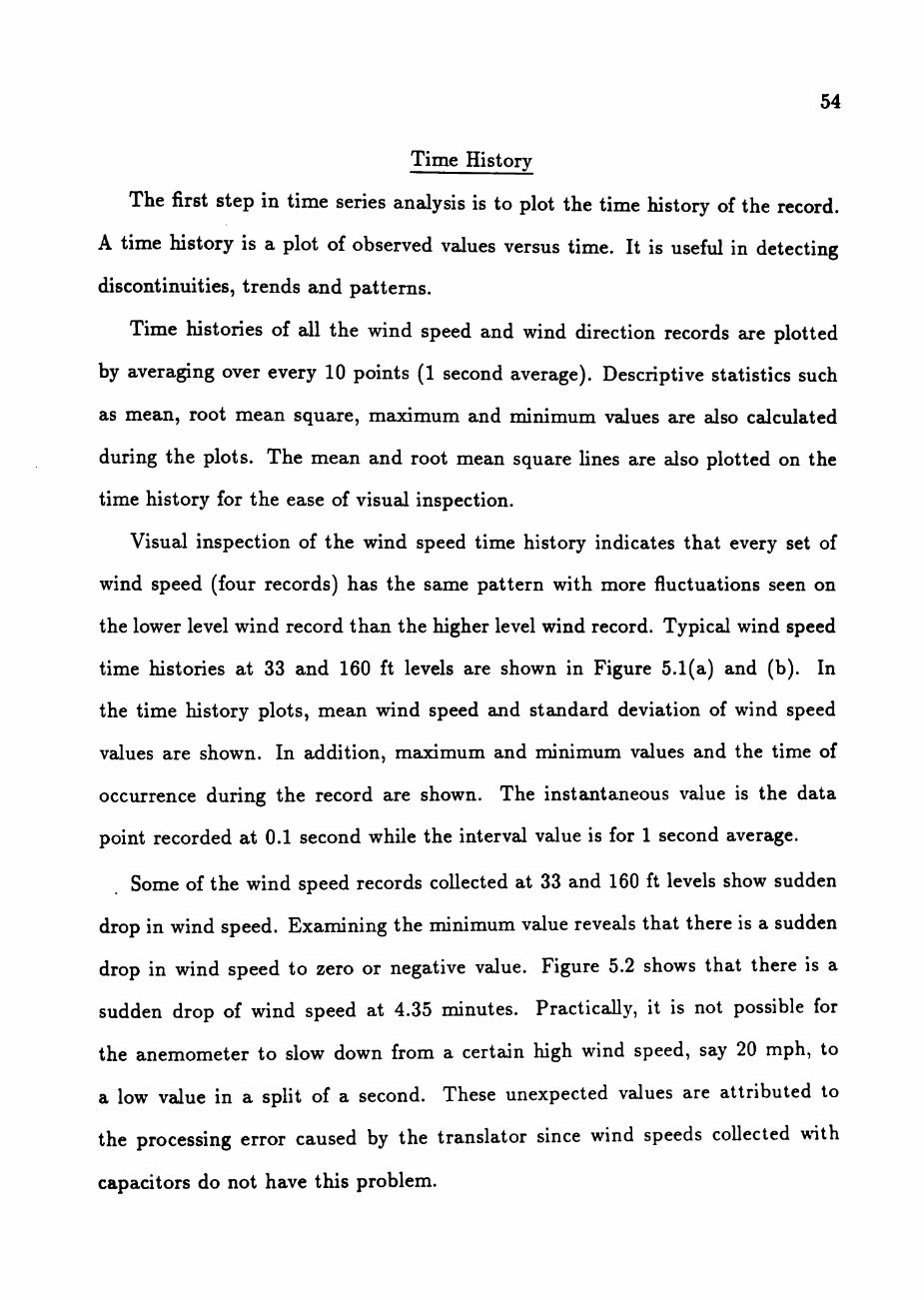
Visual inspection of the wind speed time history indicates that every set of

wind speed (four records) has the same pattern with more fluctuations seen on

the lower level wind record than the higher level wind record. Typical wind speed

time histories at 33 and 160 ft levels are shown in Figure 5.1(a) and (b). In

the time history plots, mean wind speed and standard deviation of wind speed

values are shown. In addition, maximum and minimum values and the time of

occurrence during the record are shown. The instantaneous value is the data

point recorded at 0.1 second while the interval vdue is for 1 second average.

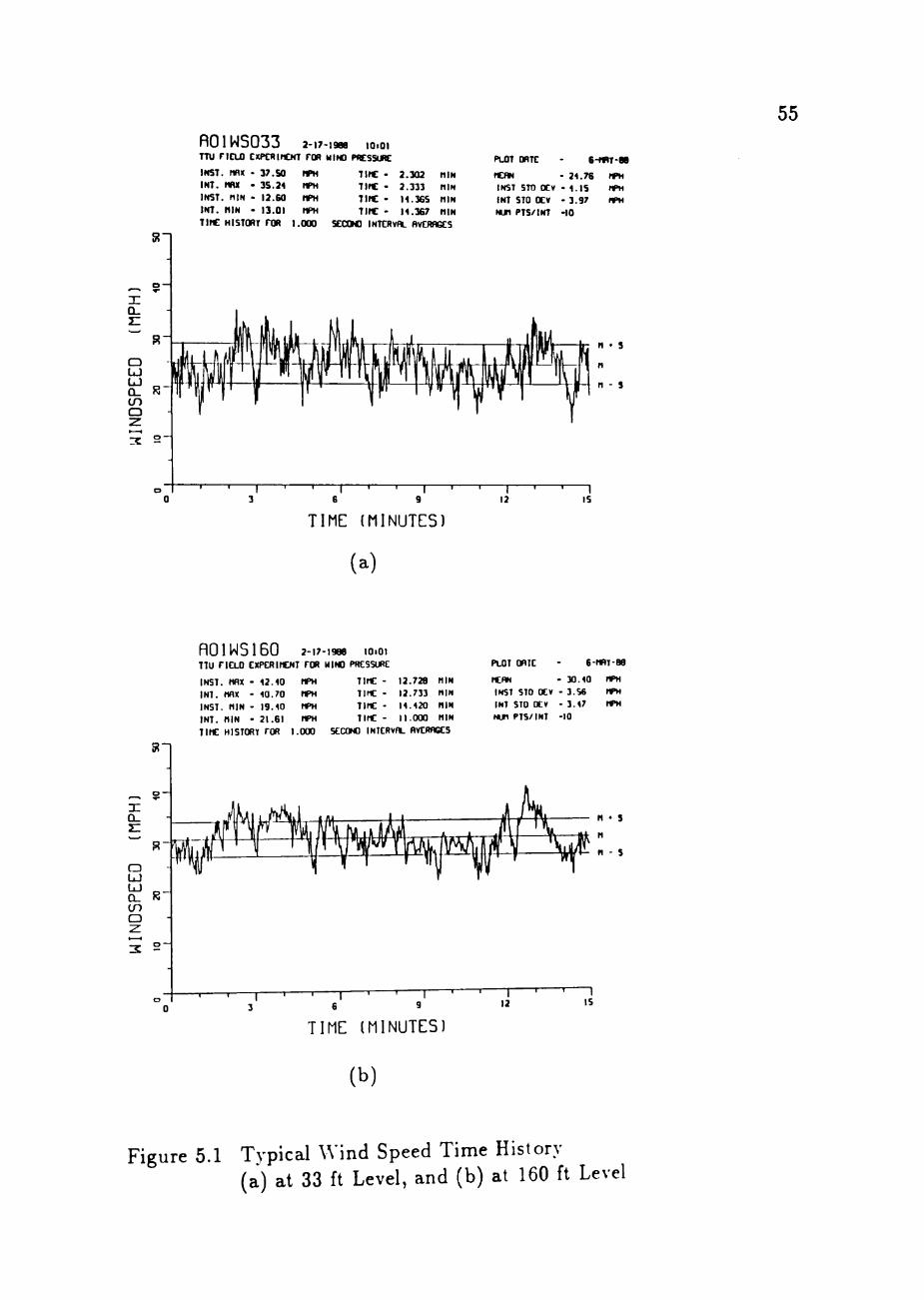
Some of the wind speed records collected at 33 and 160 ft levels show sudden

drop in wind speed. Examining the minimum value reveals that there is a sudden

drop in wind speed to zero or negative value. Figure 5.2 shows that there is a

sudden drop of wind speed at 4.35 minutes. Practically, it is not possible for

the anemometer to slow down from a certain high wind speed, say 20 mph, to

a low value in a spHt of a second. These unexpected values are attributed to

the processing error caused by the translator since wind speeds collected ^^ th

capacitors do not have this problem.

55 R01WS033 2-17-1988 lOiOl TTU riELO EXFCRIMO

IHST. tIflX - 37.50 INT. «W - 35.21 INST. tllN - 12.60 INT. niN • 13.01

n roR HI NPH HPM HPH nPH

« PfCSSURC

TIfC -TIfC -Tinc -TItC -

2.302 2.331 M.36S M.367

niN niN niN niN

PLOT QHTE 6-f«)T-aa

fCHN - 21.76 HM INST STO OCV - 1.IS nPM INT STO OCV • 3.97 nPM NUfI PTS/INT -10

TIfC HISTORT rOR 1.000 SECOWJ iNTCRVft. 8VDWGCS

TIME (MINUTES)

(a)

n O l W S l B O 2-17-1988 10.01 TTU riCLO EXPtRirCNT rOR MINO PRCSSURC

INST. MAX - 12.10 INT. nnx - 10.70 INST. MIN - 19.10

INT. nIN - 21.61

MPH MPH MPH MPH

TIME -

TIME -

TIME -

TIME -

12.728 MIN 12.733 MIN

11.120 MIN 11.000 HIN

PLOT OflIC - 6-Mni-88

fCHN - 30.10 MPH INST STO OCV - 3.56 MPH INT STO Kv - 3.17 rrn Nir PTS/INT -10

TIME HISTORT rOR 1.000 SECOND INIERVflL flVCRflCES

X Q_

r:

a UJ LJ D_ in a

T T 6 9

TIME (MINUTES: 12 IS

(b)

Figure 5.1 Typical Wind Speed Time History (a) at 33 ft Level, and (b) at 160 ft Level

56

n 2 1 W S 0 3 3 3-10-1988 13109 TTU FIELD EXPERIMENT FOR UINO PRESSURE

INST. MAX - 13.90 MPH

INT. riflX - 11.3S MPH INST. MIN —89.10 MPH INT. MIN - 8.98 MPH TIME HISTORT FOR 1.000

TIME -TIME -TIME -TIME -

12.092 MIN 12.100 MIN

1.3S0 MIN 1.3S0 MIN

SCCONO INTERVAL RVERflGES

PLOT OflTE - 5-MflY-88

MERN - 27.81 MPH

INST STO OEV - S.68 MPH INT STO OCV - 5.19 MPH NUM PTS/INT -10

TIME (MINUTES)

Figure 5.2 Wind Speed Record with Defected Data

57

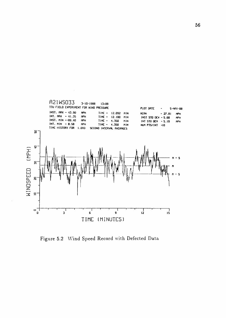
Typical time histories of the wind direction records are shown in Figure 5.3.

The time history of wind direction at 160 ft level is smoother than that at 33 ft

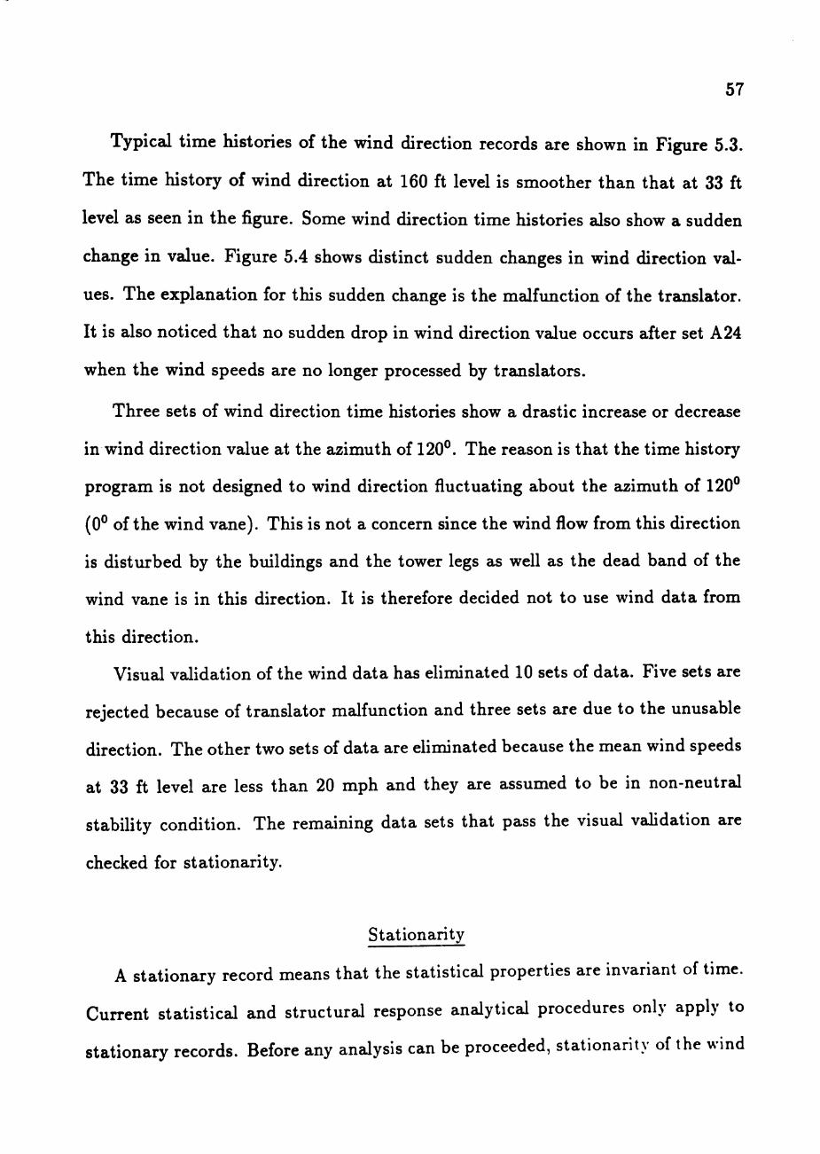
level as seen in the figure. Some wind direction time histories also show a sudden

change in value. Figure 5.4 shows distinct sudden changes in wind direction val­

ues. The explanation for this sudden change is the malfunction of the translator.

It is also noticed that no sudden drop in wind direction value occurs after set A24

when the wind speeds are no longer processed by translators.

Three sets of wind direction time histories show a drastic increase or decrease

in wind direction value at the azimuth of 120°. The reason is that the time history

program is not designed to wind direction fluctuating about the azimuth of 120°

(0° of the wind vane). This is not a concern since the wind flow from this direction

is disturbed by the buildings and the tower legs as well as the dead band of the

wind vane is in this direction. It is therefore decided not to use wind data from

this direction.

Visual validation of the wind data has eHminated 10 sets of data. Five sets are

rejected because of translator malfunction and three sets are due to the unusable

direction. The other two sets of data are eHminated because the mean wind speeds

at 33 ft level are less than 20 mph and they are assumed to be in non-neutral

stabihty condition. The remaining data sets that pass the visual validation are

checked for stationarity.

Stationarity

A stationary record means that the statistical properties are invariant of time.

Current statistical and structural response analytical procedures only apply to

stationary records. Before any analysis can be proceeded, stationarity of the wind

58 n25WD033 3-10-1988 ,6.39 TTU riCLO CXPCHIMCNT TOR UlNO PHCSSUC

INST, nnx - 26S.O0 oca INT. HRX - 2S2.SO U.U INST, MIN - 193.00 mo I N T . niN • 201.80 OLD

PLOT OHTC TIME -TIME -TIME • TIME -

12-Mni-aa B.6S3

7.913

13.992

2.200

MIN

MIN

MIN

MIN TIME HISTORT rUR I.QUO SCCONO iNTCHVtt. HVCHRGES

"CAN - 229.92 OES

INST STO DEV - B . B S ULG

I N I STO OLV • 7 . 7 9 QCG

Nm PTs/iNi -10

6 9

TIME (MINUTES)

(a)

fl25WD160 3-10-1988 I6i39 TTU riELO EXPERIMEN

INST, nnx • 261.00 INT. MAX - 2SI.60 INST. MlN - 206.00 INT. MIN • 212.SO

T rOR HIM

OEO OEG 0E6 OEG

) PRESSUIE

TIME -TIME -TIME -TIME -

6.IS2 S.200 12.187 12.183

MIN MIN MIN MIN

PLOT OHTE - l2-nni-8l

MEAN - 230.6S OEG INST STO ttv - 7.31 OEG INT STO OEV - 6.61 OEG Ntfl PTS/INT -10

TIME HISTORT TOR 1.000 SECONO INTERVrt. RvERflCES

'M»$f^l[

TIME (MINUTES)

(b)

Figure 5.3 Typical Wind Direction Time History (a) at 33 ft Level, and (b) at 160 ft Level

59

R 2 1 W D 1 6 0 3-I0-I900 13.09 TTU riCLO EXfERIIlCNT FOR UINO PRESSURE

INST. Mnx - 275.00 OCG TIME -

INT. Mnx - 2G6.90 OEG TIME -

INST. MIN —633.00 OEG TIME -

INT. MIN - 127.20 OEG TIME -

0.107

0.117

11.007

11.900

MIN MIN MIN MIN

PLOT oniE - I? MOT-no

MCnN - 220.09 OCG INST STO DEV - 17.99 OCG INT STO OEV - 9.80 OCG NUM PTS/INT -10

R_ TIME HISTORY FOR 1.000 SCCONO INTCRVOL nvEROGCS

CD UJ g

a

O u> •

CJ o — LJ " ct: H Q 5.

o 2Z o

ID •

O rsi —

W/W^k (Jv^ . .; v,. A .-/'"A^^^^^^ g;

-, . 1 1 1 1 . . I 3 G 9

- | , r 12 IS

TIME (MINUTES)

Figure 5.4 Wind Direction Record with Defected Data

60

sire speed and wind direction records should be checked. Both run and trend tests

used to check the fluctuation and trend of the wind speed. Only the trend test

is used to check the trend of wind direction record since a large trend will make

the mean wind direction meaningless. A trend exists when there is a sudden or

a continuous change of wind direction during the 15-minute period of the record.

The mean wind direction will not be representative of the predominant direction

as there may be more than one or no predominant direction. Hence, the mean of

the nonstationary wind direction record is not usable.

Both the run and trend tests require the record to be divided into independent

intervals. The interval size is determined by the autocorrelation function com­

puted using Equation (2.2). The autocorrelation function of all wind speed and

wind direction records are calculated using 120 seconds (1200 data points) and

are plotted for visual inspection. A typical wind speed autocorrelation function

plot is shown in Figure 5.5. The autocorrelation fimction fluctuates randomly and

never dies off to exactly zero, but will reach a point where it fluctuates about zero

at very small values. The point where the autocorrelation function first becomes

zero is assumed to be the die off point. The die off point for the plot in Figure

5.5 is 40 seconds. Any point beyond the die off point has httle or no correlation.

Hence, the die off point is assumed to be the minimum independent interval size.

Autocorrelation function plots of all the wind speed records show that most

of the autocorrelation function die off in the range of 35 to 70 seconds. Some of

the autocorrelation function do not die off before 120 seconds, and those records

are more Hkely to be nonstationary. Interval sizes of 45, 56 and 75 seconds which

correspond to 20, 16 and 12 intervals in 15-minute duration records, are chosen

to check the stationarity of wind speed records. These interval sizes are similar to

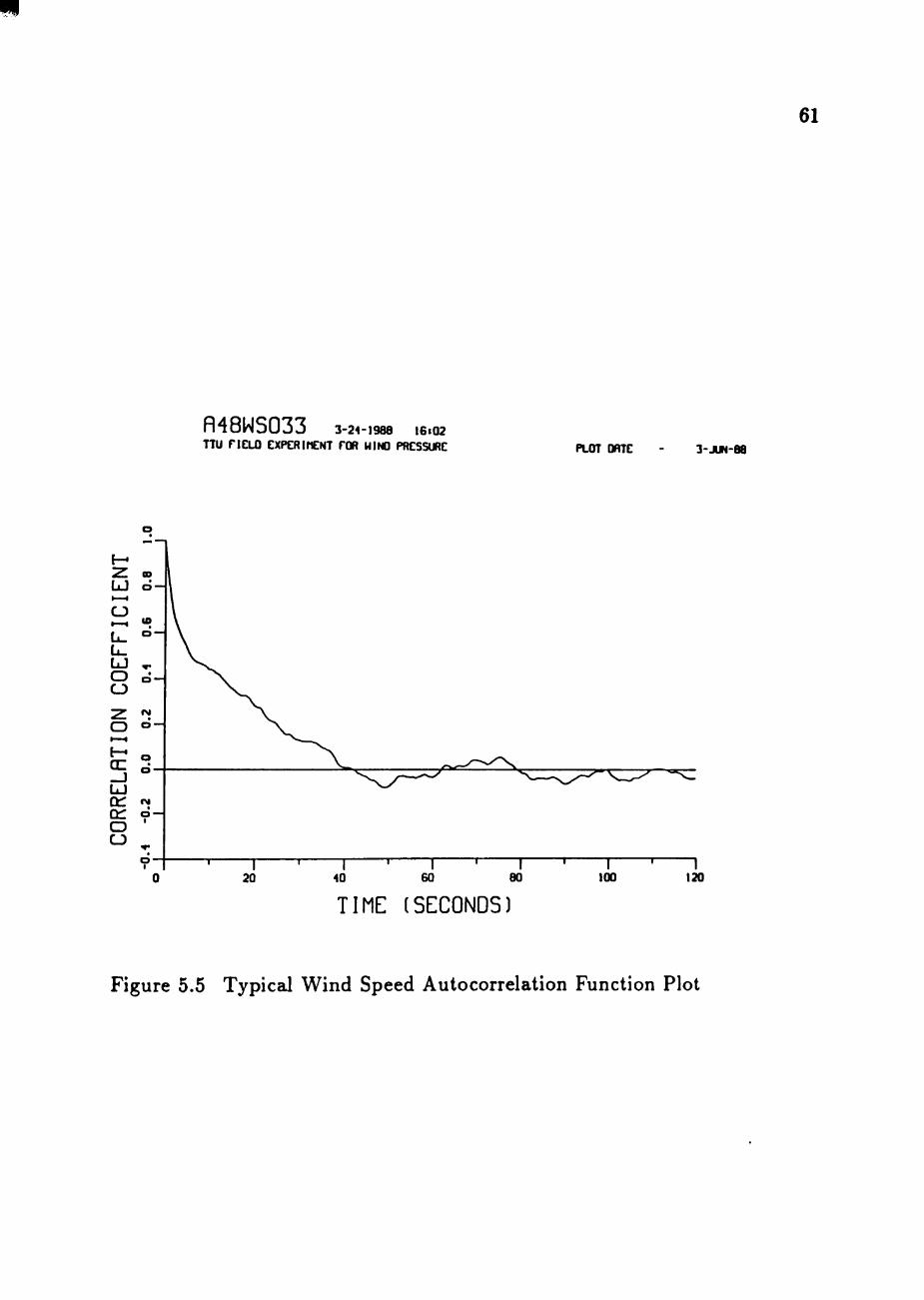
61

R48WS033 3-21-1988 I6i02 TTU riELO EXPERIMENT FOR HINO PRESSURE PLOT GATE 3-JUN-88

TIME (SECONDS)

Figure 5.5 Typical Wind Speed Autocorrelation Function Plot

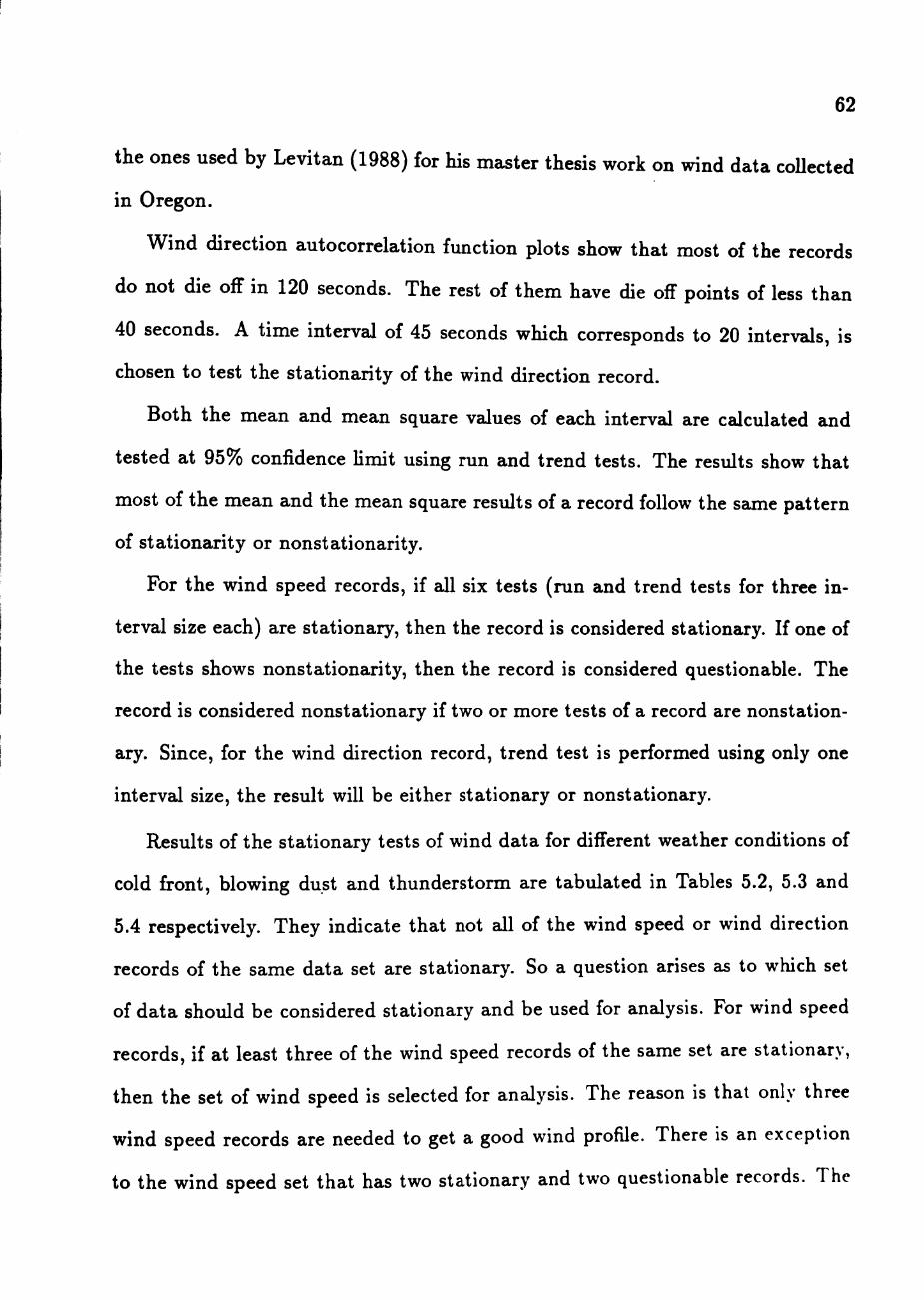
62

the ones used by Levitan (1988) for his master thesis work on wind data collected

in Oregon.

Wind direction autocorrelation function plots show that most of the records

do not die off in 120 seconds. The rest of them have die off points of less than

40 seconds. A time interval of 45 seconds which corresponds to 20 intervals, is

chosen to test the stationarity of the wind direction record.

Both the mean and mean square values of each interval are calculated and

tested at 95% confidence hmit using run and trend tests. The results show that

most of the mean and the mean square results of a record follow the same pattern

of stationarity or nonstationarity.

For the wind speed records, if all six tests (run and trend tests for three in­

terval size each) are stationary, then the record is considered stationary. If one of

the tests shows nonstationarity, then the record is considered questionable. The

record is considered nonstationary if two or more tests of a record are nonstation­

ary. Since, for the wind direction record, trend test is performed using only one

interval size, the result will be either stationary or nonstationary.

Results of the stationary tests of wind data for different weather conditions of

cold front, blowing dust and thunderstorm are tabulated in Tables 5.2, 5.3 and

5.4 respectively. They indicate that not all of the wind speed or wind direction

records of the same data set are stationary. So a question arises as to which set

of data should be considered stationary and be used for analysis. For wind speed

records, if at least three of the wind speed records of the same set are stationary,

then the set of wind speed is selected for analysis. The reason is that only three

wind speed records are needed to get a good wind profile. There is an exception

to the wind speed set that has two stationary and two questionable records. The

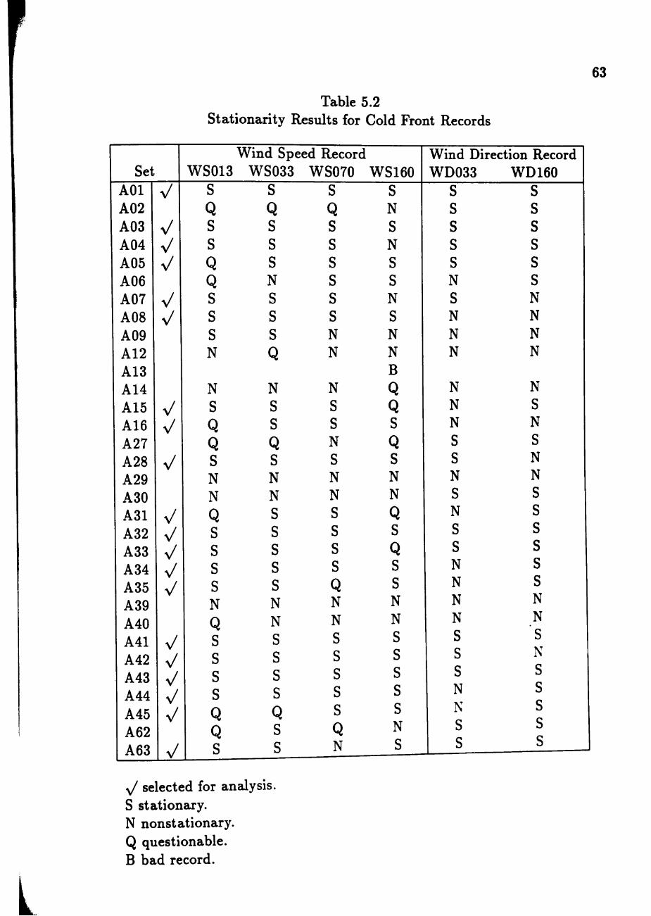
63

Table 5.2 Stationarity Results for Cold Front Records

Set AOl A02 A03 A04 A05 A06 A07 A08 A09 A12 A13 A14 A15 A16 A27 A28 A29 A30 A31 A32 A33 A34 A35 A39 A40 A41 A42 A43 A44 A45 A62 A63

^/

^/

y/

y/

y/

x/

V v/

V

V y/

x/ y/

y/

y/

y/

v/ v/ y/

J

Wind Speed Record WS013 WS033 WS070

S S S Q Q Q s s s s s s Q S S Q N S S S S S S S S S N N Q N

N N N s s s Q S S Q Q N s s s N N N N N N Q S S s s s s s s s s s S S Q N N N Q N N s S s s s s s s s s s s Q Q S Q S Q S S N

y/ selected for analysis. S stationary. N nonstationary. Q questionable. Bba id re cord.

WS160 S N S N S S N S N N B Q Q S Q s N N Q s Q s s N N S S s s s N s

Wind Direction Record WD033

S S S S S N S N N N

N N N S S N S N S S N N N N S S s N N S S

WD160 S S S S S S N N N N

N S N S N N S S s s s s N _N s N S S S c S S

L

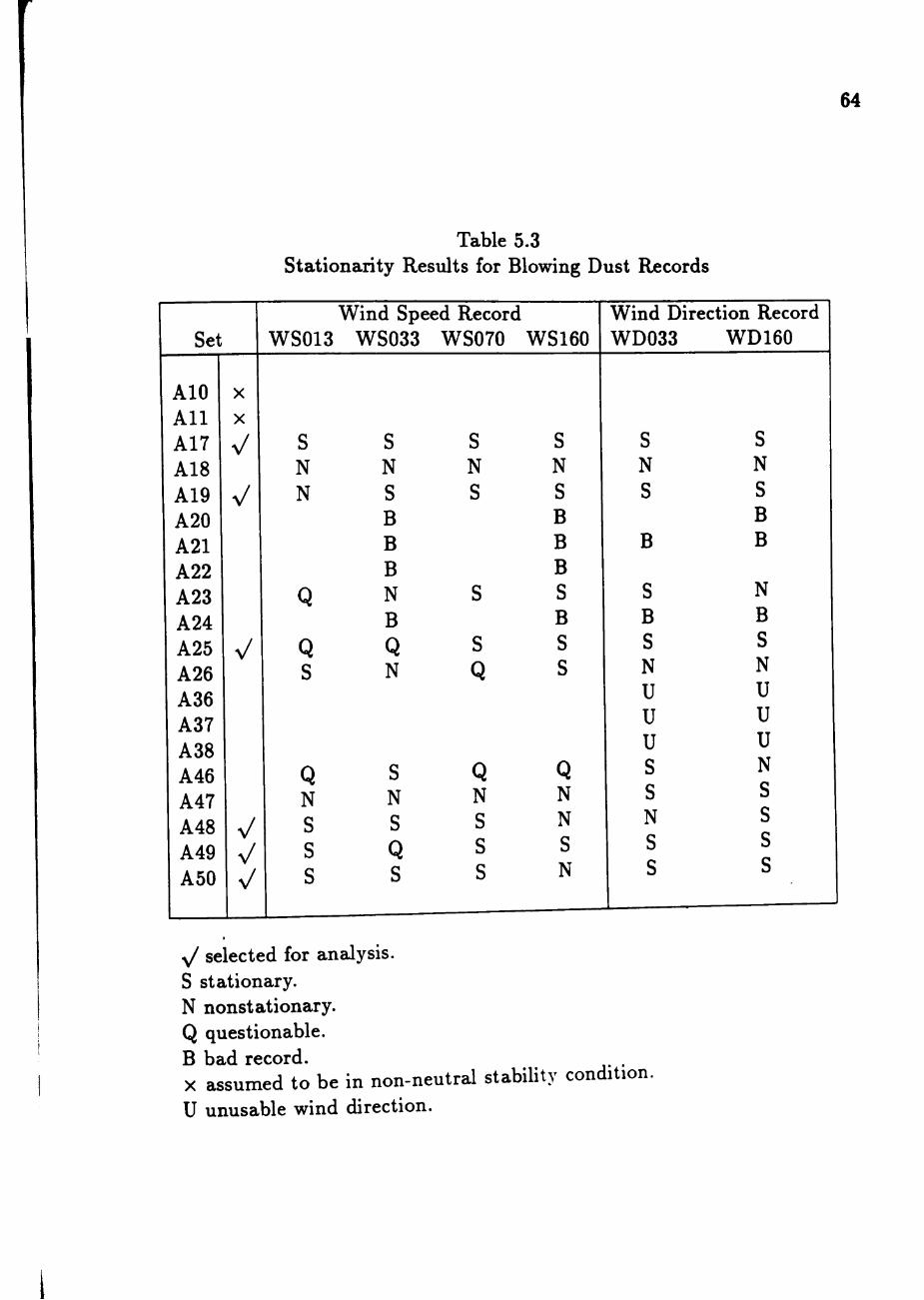
64

Table 5.3 Stationarity Results for Blowing Dust Records

Set

AlO Al l A17 A18 A19 A20 A21 A22 A23 A24 A25 A26 A36 A37 A38 A46 A47 A48 A49 A50

X

X

V

x/

y/

v/ v/ x/

WS013

S N N

Q

Q s

Q N S s s

Wind Speed Record WS033 WS070

S S N N S S B B B N S B Q S N Q

S Q N N s s Q s s s

WS160

S N S B B B S B S S

Q N N S N

Wind Direction Record WD033 WD160

S S N N s s

B B B

S N B B s s N N u u u u u u S N S s N S s s s s

y/ selected for analysis. S stationary. N nonstationary. Q questionable. B bad record. . X assumed to be in non-neutral stabihty condition. U unusable wind direction.

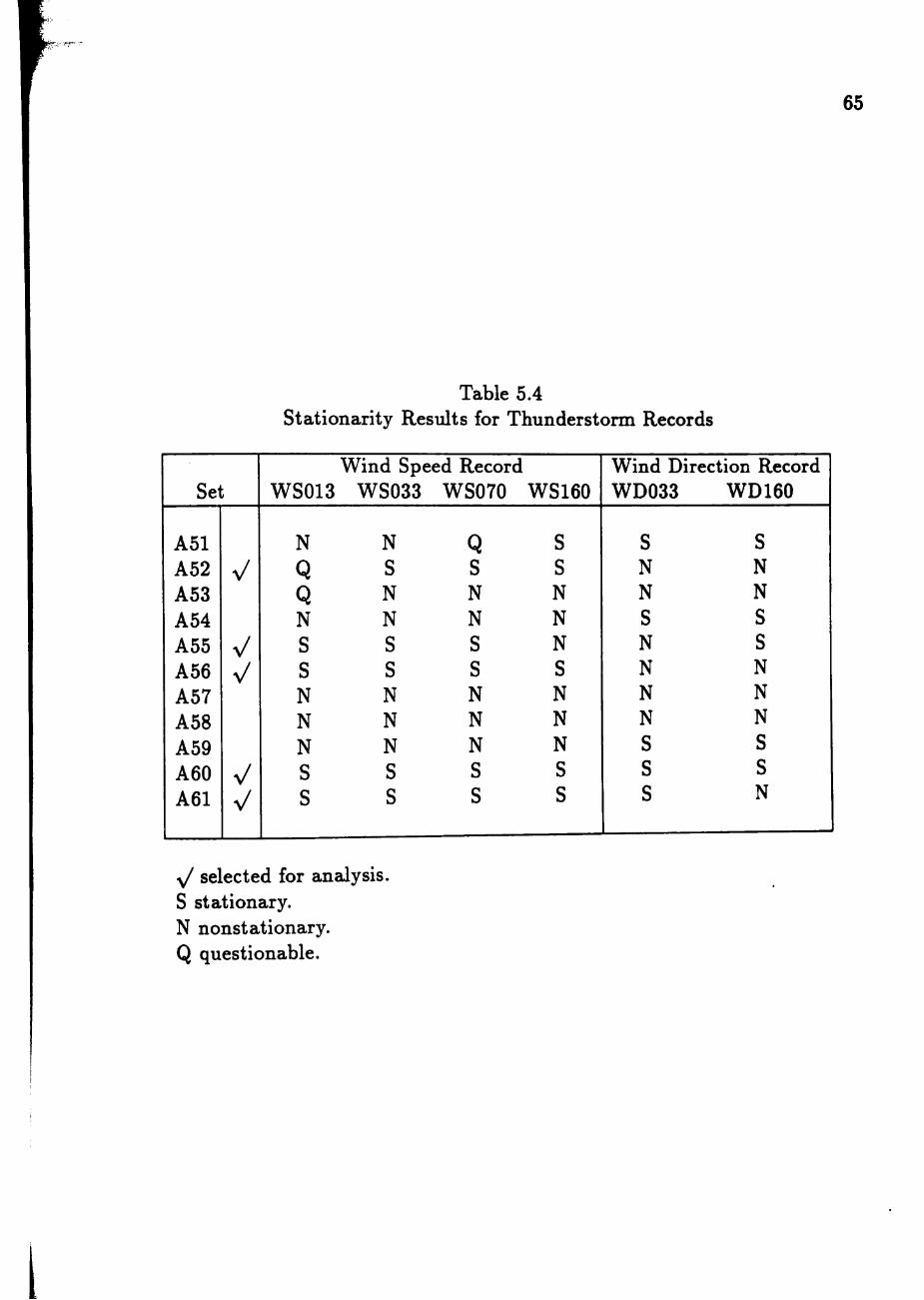
65

Table 5.4 Stationarity Results for Thunderstorm Records

Set

A51 A52 A53 A54 A55 A56 A57 A58 A59 A60 A61

V

y/

y/

y/

y/

WS013

N

Q Q N S s N N N S s

Wind Speed Record WS033 WS070

N Q s s N N N N S S s s N N N N N N s s s s

WS160

S S N N N S N N N S S

Wind Direction Record WD033 WD160

S S N N N N S S N S N N N N N N S S S S S N

y/ selected for analysis. S stationary. N nonstationary. Q questionable.

I

66

time histories of those wind records are examined to see whether they appear to

be stationary; that is the mean and fluctuation have no obvious trend. Only three

data sets require this exception.

The criterion for selecting wind direction record is if one of the wind directions

is stationary, then the data set is used for analysis. The logic behind this is that

only one wind direction is required since both the mean wind directions do not

vary much. In some cases, all the wind speed records are stationary, but both the

mean wind direction records are nonstationary, so the time histories of the wind

direction records are examined again. If most of the trend of the wind direction

record is within one root mean square and the trend does not have a sudden

change, then the wind direction set is used. A typical example is shown in Figure

5.6, which is tested to be nonstationary, but most of the trend is within one root

mean square. So it is accepted for analysis.

The stationarity test results show that about 60% of the good frontal wind

speed sets are stationary whereas less than 50% of the thunderstorm wind speed

sets are stationary. The percentage of stationary wind speed sets for the blowing

dust condition is in between the percentage of the cold front and thunderstorm

conditions. There is no clear correlation between stationarity and weather condi­

tion.

Descriptive Statistics

Mean and root mean square (RMS) values of the 31 sets of stationary wind

data are calculated. Table 5.5 shows the mean and RMS values of wind speed at

four different levels. The mean wind speed values of the same set increase with

height. The RMS value of wind speed records increases from 13 ft level to 33 ft

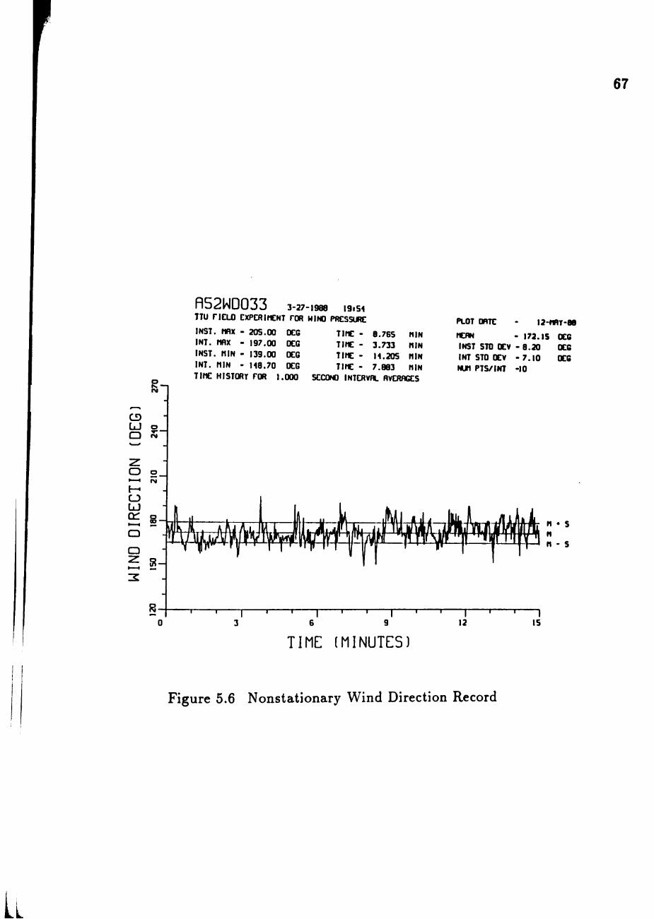
f 67

R52ND033 3-27-1988 tgisi TTU riELO EXPERIMENT FOR HINO PRESSURE

INST, tmx - 20S.00 OEG INT. MflX - 197.00 OEG INST. MIN - 139.00 X 6 INT. MIN - M8.70 OEG

TIME -TIME -TIME -TIME -

a.76S MIN 3.733 niN I1.20S niN 7.883 NIN

TIME HISTORT FOR 1.000 SCCONO INTERVRL RVERRGES

PLOT OflTE - l2-nRT-8e

"EflN - 172. IS OEG INST STO OEV - 8.20 K 6 INT STO XV -7 .10 KG NUn PTS/INT -10

CD LJ o .

r*

CJ LiJ

^ g-Q

Q

^ S -

R-12 IS

TIME (MINUTES)

Figure 5.6 Nonstationary Wind Direction Record

LL

!

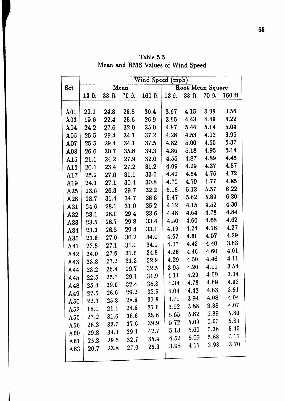
68

Table 5.5 Mean and RMS Values of Wind Speed

Set

AOl A03 A04 A05 A07 A08 A15 A16 A17 A19 A25 A28 A31 A32 A33 A34 A35 A41 A42 A43 A44 A45 A48 A49 A50 A52 A55 A56 A60 A61 A63

Wind Speed (mph)

13 ft

22.1 19.6 24.2 25.5 25.5 26.6 21.1 20.1 25.2 24.1 23.6 28.7 24.6 23.1 23.5 23.3 23.6 23.5 24.0 23.8 23.2 22.5 25.4 22.5 22.3 18.1 27.2 28.3 29.8 25.3 20.7

Mean 33 ft

24.8 22.4 27.6 29.4 29.4 30.7 24.2 23.4 27.6 27.1 26.3 31.4 28.1 26.0 26.7 26.5 27.0 27.1 27.6 27.2 26.4 25.7 29.0 26.0 25.8 21.4 31.6 32.7 34.3 29.6 23.8

70 ft

28.5 25.6 32.0 34.1 34.1 35.8 27.9 27.2 31.1 30.4 29.7 34.7 31.0 29.4 29.8 29.4 30.2 31.0 31.5 31.3 29.7 29.1 32.4 29.2 28.8 24.8 36.6 37.6 39.1 32.7 27.0

160 ft

30.4 26.9 35.0 37.2 37.5 39.3 32.0 31.2 33.0 30.8 32.2 36.6 35.2 33.6 33.4 33.1 34.0 34.1 34.8 32.9 32.5 31.9 35.8 32.5 31.9 27.0 38.6 39.9 42.7 35.4 29.3

Root Mean Square 13 ft

3.67 3.95 4.97 4.28 4.82 4.86 4.55 4.09 4.42 4.72 5.18 5.47 4.12 4.48 4.50 4.19 4.62 4.07 4.26 4.29 3.95 4.11 4.38 4.04 3.71 3.92 5.65 5.72 5.13 4.52 3.98

33 ft

4.15 4.43 5.44 4.53 5.00 5.18 4.87 4.29 4.54 4.79 5.13 5.62 4.15 4.64 4.60 4.24 4.60 4.43 4.46 4.50 4.20 4.20 4.78 4.42 3.94 3.88 5.82 5.69 5.60 5.09 4.11

70 ft

3.99 4.49 5.14 4.02 4.65 4.95 4.89 4.37 4.76 4.77 5.57 5.89 4.52 4.78 4.68 4.18 4.57 4.40 4.60 4.46 4.11 4.09 4.69 4.63 4.08 3.88 5.89 5.63 5.36 5.68 3.98

160 ft

3.56 4.22 5.04 3.95 5.37 5.14 4.45 4.57 4.72 4.85 6.22 6.30 4.30 4.84 4.62 4.27 4.29 3.83 4.01 4.11 3.54 3.34 4.03 3.91 4.04 4.07 5.80 5.84 5.45 5.17 3.<0

r 69

level; then decreases with height. The RMS value at 33 ft level is higher than

that at 13 ft level by 0.2 to 0.4 mph in most of the data sets. Higher RMS value

means more turbulence. More turbulence at 33 ft level than at 13 ft level seems

unrealistic because ground roughness generates more turbulence at 13 ft level than

at 33 ft level during high wind condition. This anomaly of higher turbulence at

33 ft level than at 13 ft level is not known.

Mean and RMS values of the wind direction are tabulated in Table 5.6. Gen­

erally, the variation of mean wind direction follows the Ekman spiral which states

that the mean wind direction increases with height in a clockwise direction (Panof­

sky and Dutton, 1986). Most of the variation of mean wind direction is from 1°

to 5°. Six of the wind direction sets show decrease of 1° to 2° in mean wind direc­

tion with height in clockwise direction respectively. Another five wind direction

sets do not show any variation of mean wind direction. The RMS values of the

wind direction decrease with height by 1° to 3° which is expected as there is less

fluctuation high above ground.

Wind Profile Parameters

The wind profile parameters power law exponent a, roughness length ZQ and

shear velocity U. are determined from the power and logarithmic laws. Both of

the a and ZQ parameters will be used to characterize the roughness of the terrain.

Power Law Parameter

The power law exponent a can be obtained by making the power law of Equa­

tion (2.4) to be hneax so that hnear regression can be performed to obtain the

best fit hne. The hnear form of the power law is :

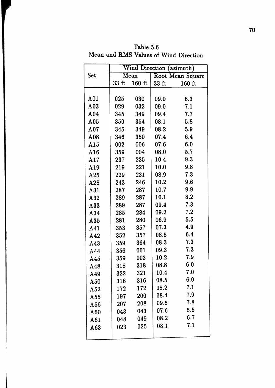
F 70

Table 5.6 Mean and RMS Values of Wind Direction

Set

AOl A03 A04 A05 A07 A08 A15 A16 A17 A19 A25 A28 A31 A32

A33 A34 A35 A41 A42 A43 A44 A45 A48 A49 A50 A52 A55 A56 A60 A61 A63

Wind Direction (azimuth) Mean

33 ft

025 029 345 350 345 346 002 359 237 219 229 243 287 289 289 285 281 353 352 359 356 359 318 322 316 172 197 207 043 048 023

160 ft

030 032 349 354

349 350 006 004 235 221 231 246 287 287 287 284 280 357 357 364 001 003 318 321 316 172 200 208 043 049 025

Root Mean Square 33 ft

09.0 09.0 09.4 08.1 08.2 07.4 07.6 08.0 10.4 10.0 08.9 10.2 10.7 10.1 09.4 09.2 06.9 07.3 08.5 08.3 09.3 10.2 08.8 10.4 08.5 08.2 08.4 09.5 07.6 08.2

08.1

160 ft

6.3 7.1 7.7 5.8 5.9 6.4 6.0 5.7 9.3 9.8 7.3 9.6 9.9 8.2 7.3 7.2 5.5 4.9 6.4 7.3 7.3 7.9 6.0 7.0 6.0 7.1 7.9 7.8 5.5 6.7 7.1

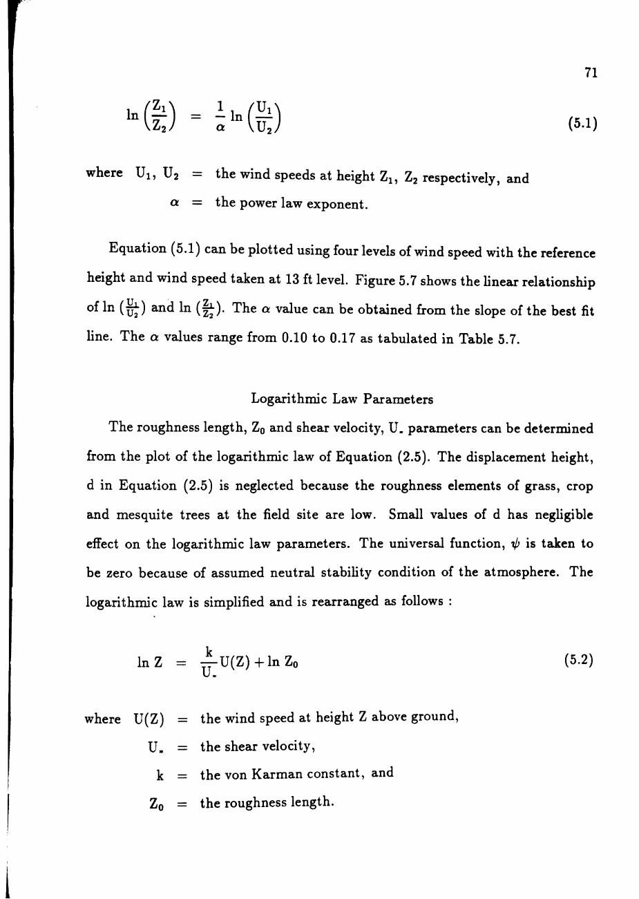
71

where Ui, U2 = the wind speeds at height Zi, Z2 respectively, and

a = the power law exponent.

Equation (5.1) can be plotted using four levels of wind speed with the reference

height and wind speed taken at 13 ft level. Figure 5.7 shows the hnear relationship

^^ ^^ (u t ) ^^^ ^^ (fe) ' '^^^ " v^^« can be obtained from the slope of the best fit

hne. The a values range from 0.10 to 0.17 as tabulated in Table 5.7.

Logarithmic Law Parameters

The roughness length, ZQ and shear velocity, U. parameters can be determined

from the plot of the logarithmic law of Equation (2.5). The displacement height,

d in Equation (2.5) is neglected because the roughness elements of grass, crop

and mesquite trees at the field site are low. Smsdl values of d has neghgible

effect on the logarithmic law parameters. The universal function, V' is taken to

be zero because of assumed neutral stabihty condition of the atmosphere. The

logarithmic law is simplified and is rearranged as follows :

InZ = : ^ U ( Z ) - h l n Z o (5.2)

where U(Z) = the wind speed at height Z above ground,

U. = the shear velocity,

k = the von Karman constant, and

Zo = the roughness length.

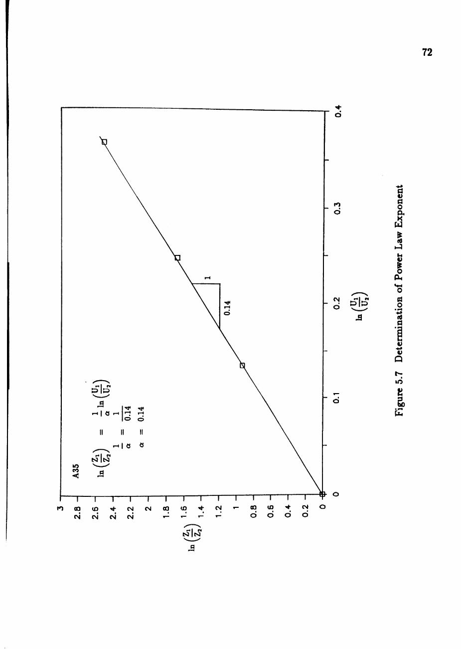
72

o

(VI

d

a a o p.

I

I O

d

Q

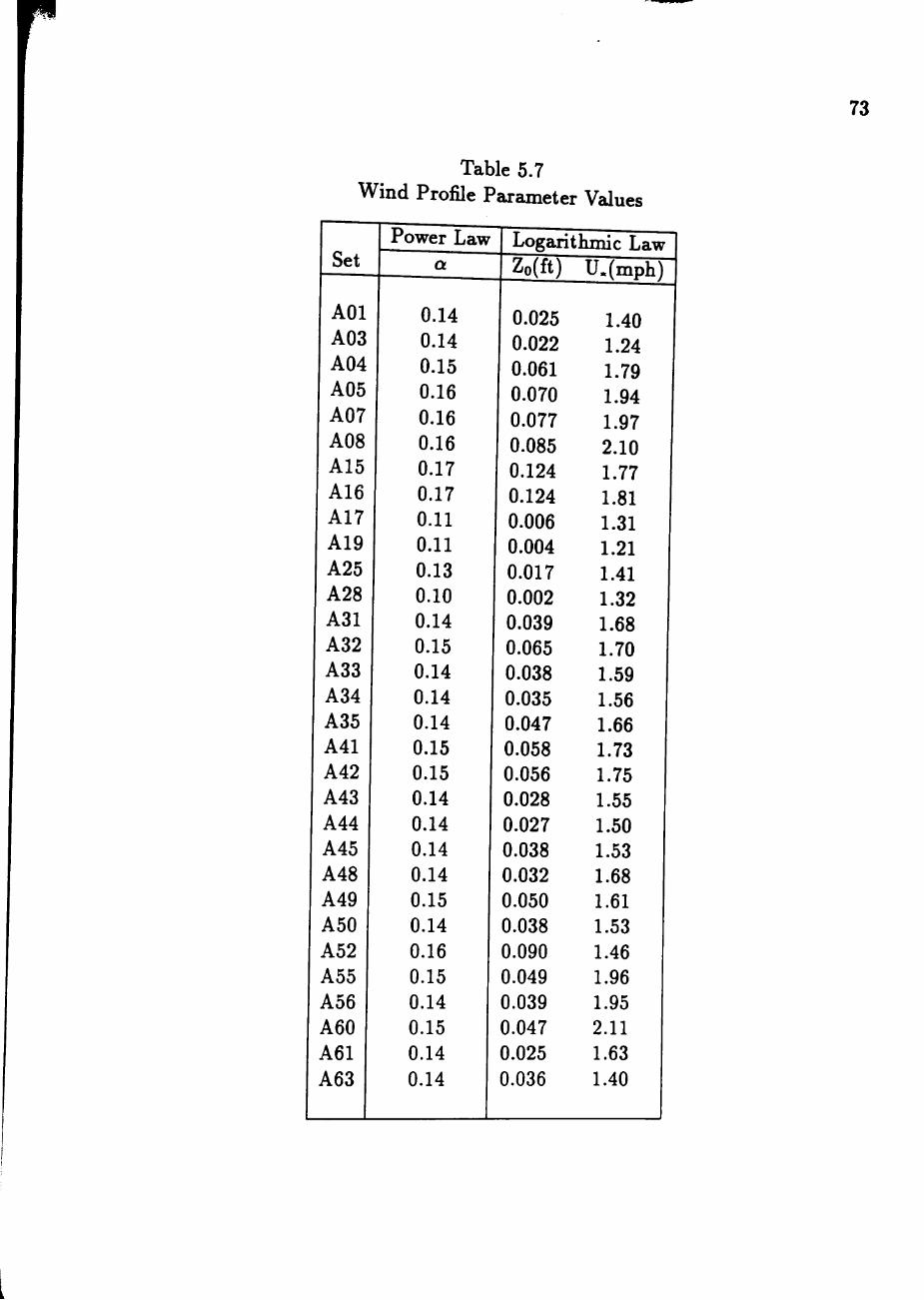
73

Table 5.7 Wind Profile Parameter Values

Set

AOl A03 A04 A05 A07 A08 A15 A16 A17 A19 A25 A28 A31 A32 A33 A34 A35 A41 A42 A43 A44 A45 A48 A49 A50 A52 A55 A56 A60 A61 A63

Power Law a

0.14 0.14 0.15 0.16 0.16 0.16 0.17 0.17 0.11 0.11 0.13 0.10 0.14 0.15 0.14 0.14 0.14 0.15 0.15 0.14 0.14 0.14 0.14 0.15 0.14 0.16 0.15 0.14 0.15 0.14 0.14

Logarithmic Law Zo(ft)

0.025 0.022 0.061 0.070 0.077 0.085 0.124 0.124 0.006 0.004 0.017

1 0.002 0.039 0.065 0.038 0.035 0.047 0.058 0.056 0.028 0.027 0.038 0.032 0.050 0.038 0.090 0.049 0.039 0.047 0.025 0.036

U.(mph)

1.40 1.24 1.79 1.94 1.97 2.10 1.77 1.81 1.31 1.21 1.41 1.32 1.68 1.70 1.59 1.56 1.66 1.73 1.75 1.55 1.50 1.53 1.68 1.61 1.53 1.46 1.96 1.95 2.11 1.63 1.40

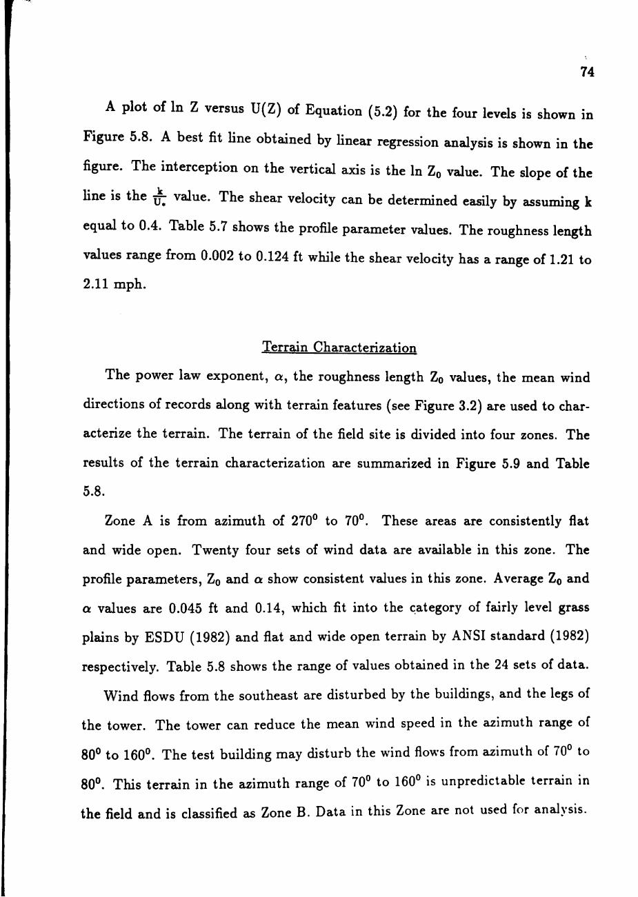
74

A plot of In Z versus U(Z) of Equation (5.2) for the four levels is shown in

Figure 5.8. A best fit hne obtained by hnear regression analysis is shown in the

figure. The interception on the vertical ajcis is the In ZQ value. The slope of the

Hne is the ^^ value. The shear velocity can be determined easily by assuming k

equal to 0.4. Table 5.7 shows the profile parameter values. The roughness length

values range from 0.002 to 0.124 ft while the shear velocity has a range of 1.21 to

2.11 mph.

Terrain Characterization

The power law exponent, a, the roughness length ZQ values, the mean wind

directions of records along with terredn features (see Figure 3.2) are used to char­

acterize the terrain. The terrain of the field site is divided into four zones. The

results of the terrain characterization axe summarized in Figure 5.9 and Table

5.8.

Zone A is from azimuth of 270° to 70°. These areas are consistently flat

and wide open. Twenty four sets of wind data are available in this zone. The

profile parameters, ZQ and a show consistent values in this zone. Average ZQ and

a values are 0.045 ft and 0.14, which fit into the category of fairly level grass

plains by ESDU (1982) and flat and wide open terrain by ANSI standard (1982)

respectively. Table 5.8 shows the range of values obtained in the 24 sets of data.

Wind flows from the southeast are disturbed by the buildings, and the legs of

the tower. The tower can reduce the mean wind speed in the azimuth range of

80° to 160°. The test building may disturb the wind flows from azimuth of 70° to

80°. This terrain in the azimuth range of 70° to 160° is unpredictable terrain in

the field and is classified as Zone B. Data in this Zone are not used for analysis.

^

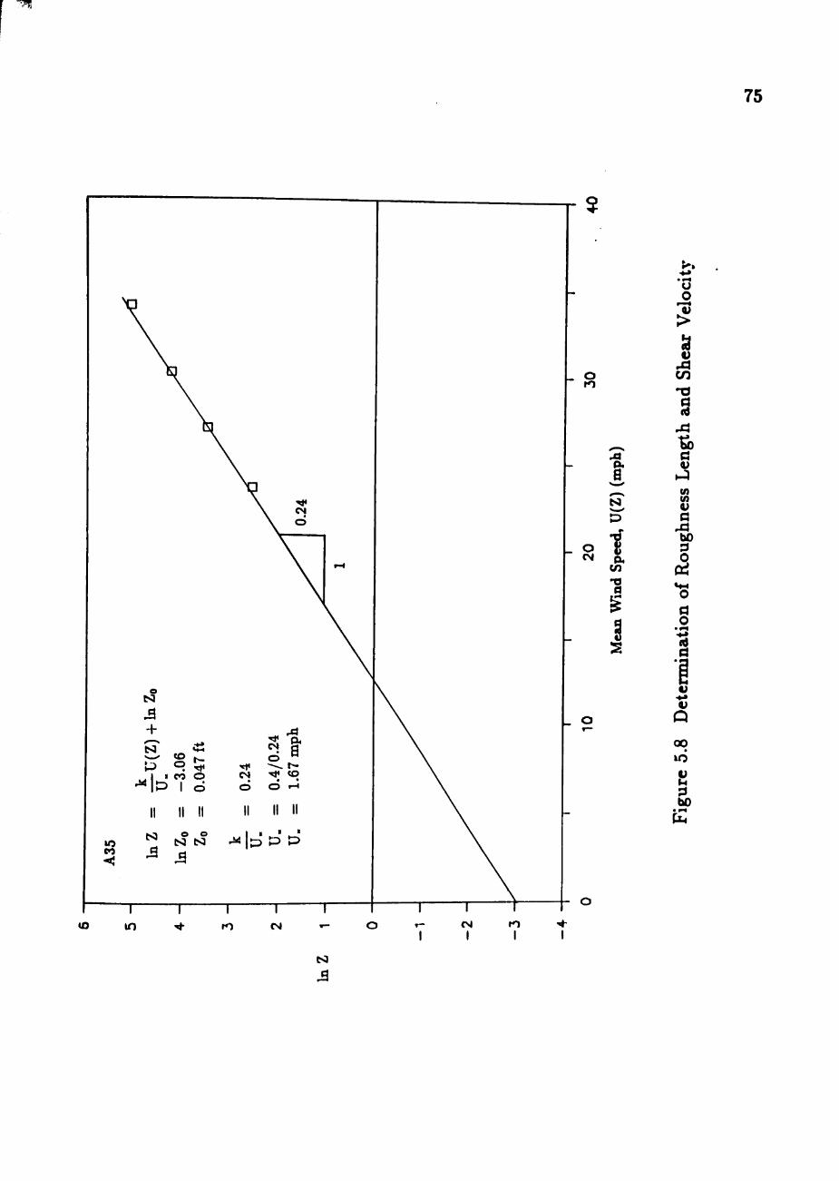
75

•>»»

o ro

N

(/I

0

e tSJ

^ 1 I CO O •«1< C<4

^ ''^ ^ A " n o ^ • -> . r -Tj« t o

II II II

o o tS3 ISJ

(O "T lO

"T T" CM

_ O

u o

a M cn a

a

w

a bO

o

d o Id d

V •*»

V

O (X)

d bO

eg I

ro

t>J

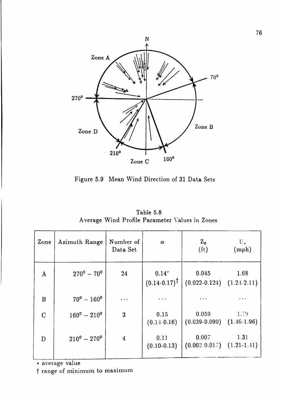
Zone A

270^

Zone D

21Q0

70°

Zone B

Zone C 160°

Figure 5.9 Mean Wind Direction of 31 Data Sets

Table 5.8 Average Wind Profile Parameter Values in Zones

Zone

A

B

C

D

Azimuth Range

270° - 70°

70° - 160°

160°-210°

210° - 270°

Number of Data Set

24

• • •

3

4

a

0.14-

(0.14-0.17)t

0.15 (0.14-0.16)

0.11 (0.10-0.13)

Zo (ft)

0.045

(0.022-0.124)

0.059 (0.039-0.090)

0.007 (0.002-0.017)

U. (mph)

1.68

(1.24 2.11)

1.7! (1.46-1.96)

1.31 (1.21-1.41)

* average value t range of minimum to maximum

77

Between azimuth range of 160° to 210°, the average Zo and a values indicate

sHghtly rougher terrain than terrain in Zone A. This area is classified as Zone C

(see Figure 5.9). The result of this zone is not conclusive due to the fact that only

three sets of wind data are available. The range of ZQ and a values are shown in

Table 5.8.

Zone D is from the direction of the playa lake in the azimuth range of 210° to

270°. The average ZQ and a values are 0.007 ft and 0.11 respectively (see Figure

5.8). The parameters distinctly indicate the smoothest terrain at the field site. It

should be pointed out that there are 14 sets of wind data collected in this zone.

Only four of them are stationary and are used to get the wind profile parameters.

The rest of them have the same wind profile parameters that distinctly show that

Zone D is the smoothest terrain.

Turbulence Intensity

The turbulence intensity can be calculated using the mean and root mean

square values of the wind speed. Equation (2.6) is used for the calculation. The

turbulence intensity values for 31 sets of data are tabulated in Table 5.9. The

turbulence intensity values decrease with height. The decrease in turbulence

intensity value from 13 ft level to 33 ft level is due to the increase in mean wind

speed. As noted previously, the RMS values for 33 ft level are higher that 13

ft level for most of the data sets (see Table 5.5). Table 5.10 shows the average

turbulence intensity values in three zones. The average turbulence intensity values

at various heights in Zone A are the lowest as compared with Zone C £md Zone

D.

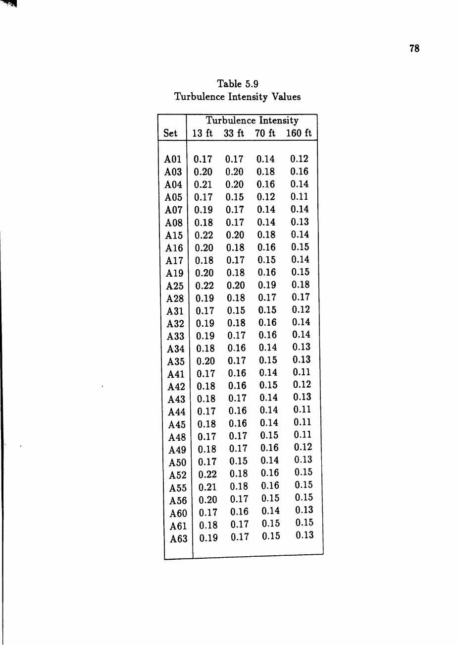
78

Table 5.9 Turbulence Intensity Values

Set

AOl A03 A04 A05 A07 A08 A15 A16 A17 A19 A25 A28 A31 A32 A33 A34 A35 A41 A42 A43 A44 A45 A48 A49 A50 A52 A55 A56 A60 A61 A63

Turbulence Intensity 13 ft

0.17 0.20 0.21 0.17 0.19 0.18 0.22 0.20 0.18 0.20 0.22 0.19 0.17 0.19 0.19 0.18 0.20 0.17 0.18 0.18 0.17 0.18 0.17 0.18 0.17 0.22 0.21 0.20 0.17 0.18 0.19

33 ft

0.17 0.20 0.20 0.15 0.17 0.17 0.20 0.18 0.17 0.18 0.20 0.18 0.15 0.18 0.17 0.16 0.17 0.16 0.16 0.17 0.16 0.16 0.17 0.17 0.15 0.18 0.18 0.17 0.16 0.17 0.17

70 ft

0.14 0.18 0.16 0.12 0.14 0.14 0.18 0.16 0.15 0.16 0.19 0.17 0.15 0.16 0.16 0.14 0.15 0.14 0.15 0.14 0.14 0.14 0.15 0.16 0.14 0.16 0.16 0.15 0.14 0.15 0.15

160 ft

0.12 0.16 0.14 0.11 0.14 0.13 0.14 0.15 0.14 0.15 0.18 0.17 0.12 0.14 0.14 0.13 0.13 0.11 0.12 0.13 0.11 0.11 0.11 0.12 0.13 0.15 0.15 0.15 0.13 0.15 0.13

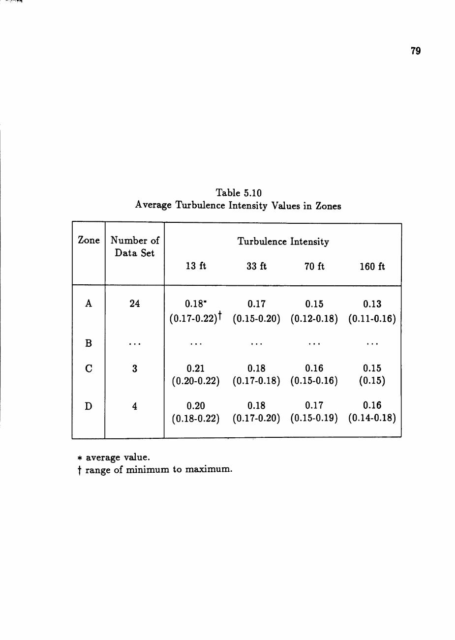
'.•w)5

Table 5.10 Average Turbulence Intensity Values in Zones

Zone

A

B

C

D

Number of Data Set

24

3

4

13 ft

0.18-(0.17-0.22)t

0.21 (0.20-0.22)

0.20 (0.18-0.22)

Turbulence Intensity

33 ft 70 ft

0.17 (0.15-0.20)

0.18 (0.17-0.18)

0.18 (0.17-0.20)

0.15 (0.12-0.18)

0.16 (0.15-0.16)

0.17 (0.15-0.19)

160 ft

0.13 (0.11-0.16)

0.15 (0.15)

0.16 (0.14-0.18)

79

* average value. t range of minimum to maximum.

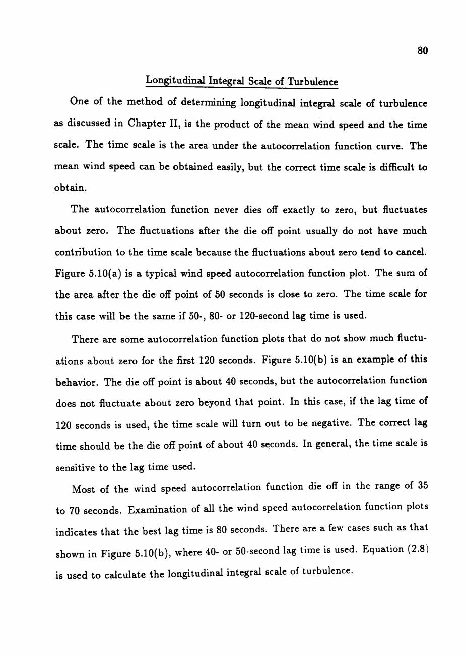
80

Longitudinal Integral Scale of Turbulence

One of the method of determining longitudinal integral scale of turbulence

as discussed in Chapter II, is the product of the mean wind speed and the time

scale. The time scale is the area under the autocorrelation function curve. The

mean wind speed can be obtained easily, but the correct time scale is difficult to

obtain.

The autocorrelation function never dies off exactly to zero, but fluctuates

about zero. The fluctuations after the die off point usually do not have much

contribution to the time scale because the fluctuations about zero tend to cancel.

Figure 5.10(a) is a typical wind speed autocorrelation function plot. The sum of

the area after the die off point of 50 seconds is close to zero. The time scale for

this case will be the same if 50-, 80- or 120-second lag time is used.

There are some autocorrelation function plots that do not show much fluctu­

ations about zero for the flrst 120 seconds. Figure 5.10(b) is an example of this

behavior. The die off point is about 40 seconds, but the autocorrelation function

does not fluctuate about zero beyond that point. In this case, if the lag time of

120 seconds is used, the time scale will turn out to be negative. The correct lag

time should be the die off point of about 40 seconds. In general, the time scale is

sensitive to the lag time used.

Most of the wind speed autocorrelation function die off in the range of 35

to 70 seconds. Examination of all the wind speed autocorrelation function plots

indicates that the best lag time is 80 seconds. There are a few cases such as that

shown in Figure 5.10(b), where 40- or 50-second lag time is used. Equation (2.8)

is used to calculate the longitudinal integral scale of turbulence.

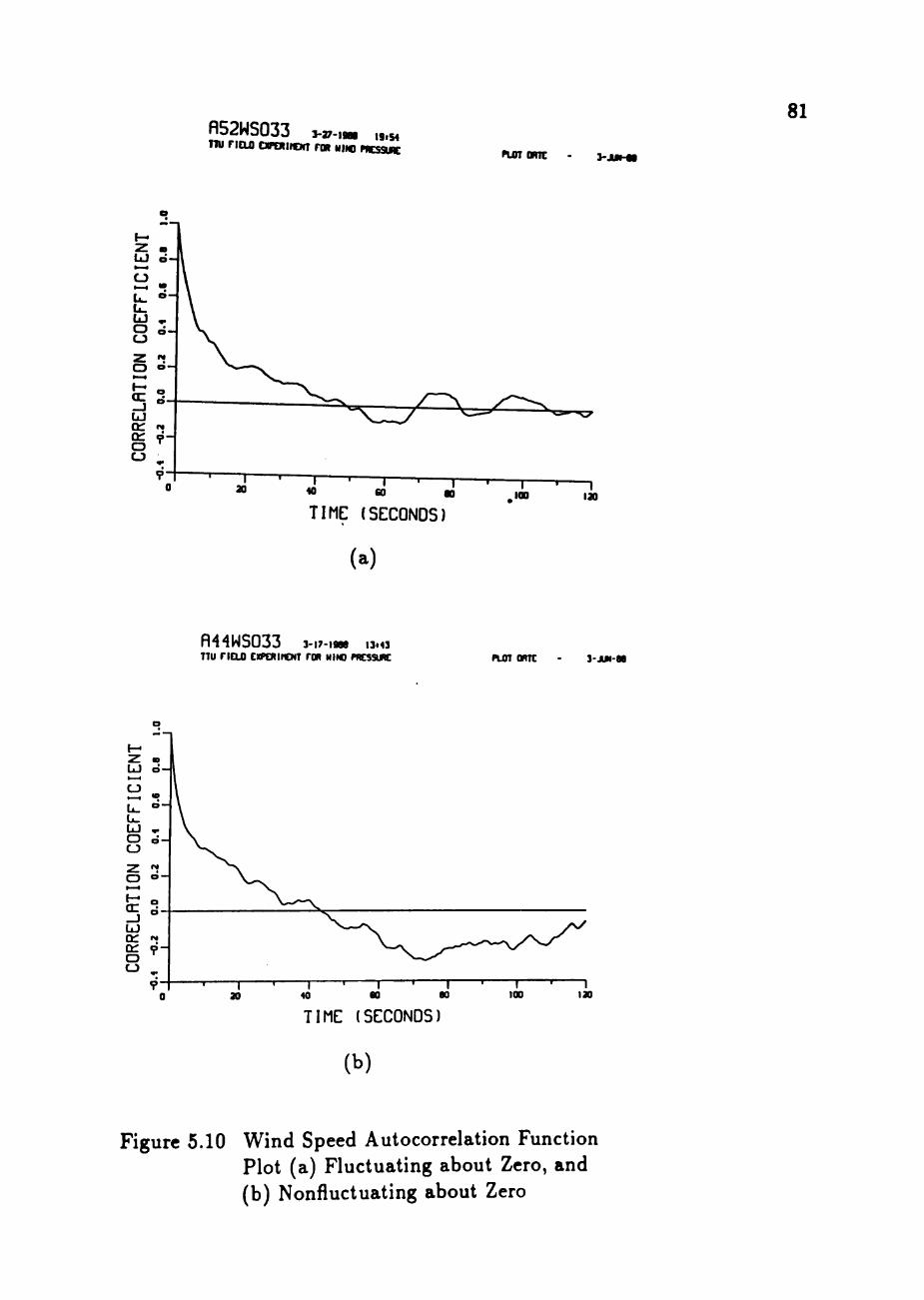
fl52WS033 j-a;-,* ,9.5, nu riofl cxPDtircNT nw uim ncssuRc

81

njOT ORTC 3-JW-M

TIME (SECONDS)

(a)

R44NS033 3-i7-i9n is.o TTU riCLO cxPCRinorr FOR HINO PRCSSUC njn OBTC ]-jui-aa

TIME (SECONDS)

(b)

Figure 5.10 Wind Speed Autocorrelation Function Plot (a) Fluctuating about Zero, and (b) Nonfluctuating about Zero

82

diie The results of the time scale and longitudinal integral scale of turbulence

tabulated in Table 5.11. The time scale increases with height, which impUes the

average duration of the effect of eddies at a point increases with height. Thus,

the longitudinal integral scale of turbulence is expected to increase with height.

Table 5.11 shows the increasing trend of longitudinal integral scale of turbulence

with height. The increase is due to the combination of increasing time scale and

mean wind speed. A larger integral scale of turbulence is formed at higher level

because there is less effect of ground roughness on the formation of large eddies.

Average values of longitudinal integral scale of turbulence in the zones are

tabulated in Table 5.12. Zone D, which has the smoothest terrain, has the highest

average value, whereas the lowest average value is in Zone C. In general, the

average longitudinal integral scale of turbulence value increases with smoother

terrain.

The average longitudinal integral scale of turbulence value at 33 ft level is

compared with other investigators' results tabulated in Table 2.3. Zone A and

Zone C average values are close to the results obt£dned over flat and open terrain

by Teunissen (1979) and Shiotani and Iwatani (1979). Zone D average value of

619 ft is close to 190 m (623 ft) by Choi (1975), 210 m (689 ft) by Mackey and Lo

(1975), and, 195 m (640 ft) by Shiotani and Iwatani (1979) which are obtained

over coastal and sea terrain.

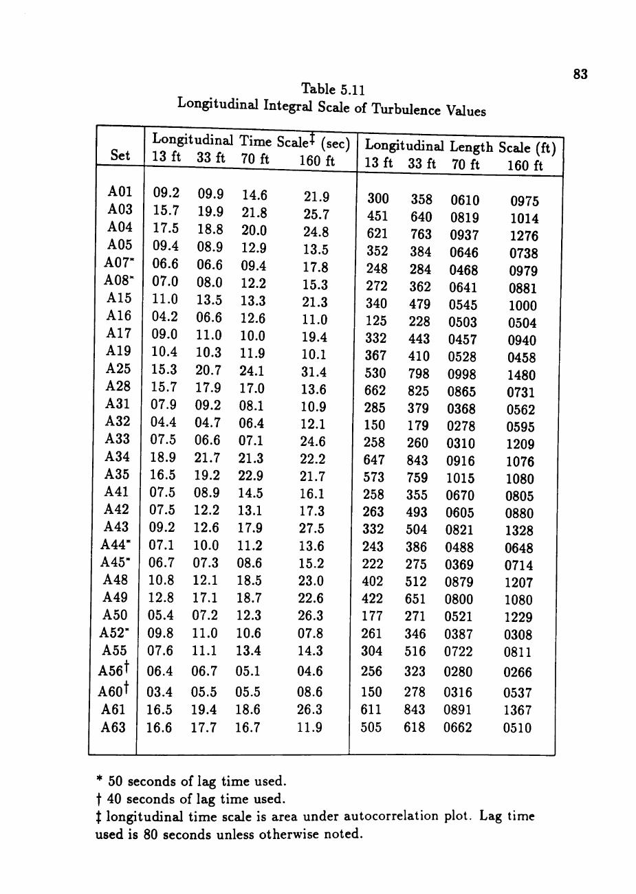
Table 5.11 Longitudinal Integral Scale of Turbulence Values

83

Set

AOl

A03 A04 A05 A07"" A08'' A15 A16 A17 A19 A25 A28 A31 A32 A33 A34 A35 A41 A42 A43 A44"' A45-A48 A49 A50 A52-A55

A56t

A60t

A61 A63

Long 13 ft

09.2

15.7 17.5 09.4 06.6 07.0 11.0 04.2 09.0 10.4 15.3 15.7 07.9 04.4 07.5 18.9 16.5 07.5 07.5 09.2 07.1 06.7 10.8 12.8 05.4

09.8 07.6

06.4

03.4 16.5 16.6

itudinal Time 33 ft 70 ft

09.9 14.6 19.9 18.8 08.9 06.6 08.0 13.5 06.6 11.0 10.3 20.7 17.9 09.2 04.7 06.6 21.7 19.2 08.9 12.2 12.6 10.0 07.3 12.1 17.1 07.2

11.0 11.1

06.7

05.5 19.4 17.7

21.8 20.0 12.9 09.4 12.2 13.3 12.6 10.0 11.9 24.1 17.0 08.1 06.4 07.1 21.3 22.9 14.5 13.1 17.9 11.2 08.6 18.5 18.7 12.3 10.6 13.4

05.1

05.5 18.6 16.7

Scaled (sec)

160 ft

21.9 25.7 24.8 13.5 17.8 15.3 21.3 11.0 19.4 10.1 31.4 13.6 10.9 12.1 24.6 22.2 21.7 16.1 17.3 27.5 13.6 15.2 23.0 22.6 26.3 07.8 14.3

04.6

08.6 26.3 11.9

Longitudinz 13 ft 33 ft

300 451 621 352 248 272 340 125 332 367 530 662 285 150 258 647 573 258 263 332 243 222 402 422 177 261 304

256

150 611 505

358 640 763 384 284 362 479 228 443 410 798 825 379 179 260 843 759 355 493 504 386 275 512 651 271 346 516

323

278 843 618

d Length 70 ft

0610 0819 0937 0646 0468 0641 0545 0503 0457 0528 0998 0865 0368 0278 0310 0916 1015 0670 0605 0821 0488 0369 0879 0800 0521 0387 0722

0280

0316 0891 0662

Scale (ft) 160 ft

0975 1014 1276 0738 0979 0881 1000 0504 0940 0458 1480 0731 0562 0595 1209 1076 1080 0805 0880 1328 0648 0714 1207 1080 1229 0308 0811

0266

0537 1367 0510

* 50 seconds of lag time used. t 40 seconds of lag time used. t longitudinal time scale is area under autocorrelation plot. Lag time used is 80 seconds unless otherwise noted.

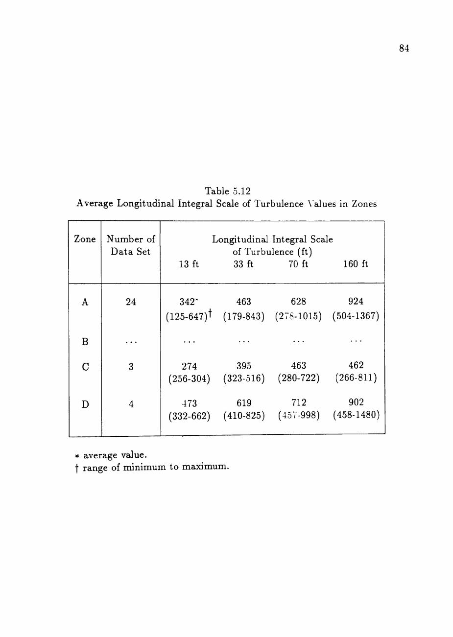
84

Table 5.12 Average Longitudinal Integral Scale of Turbulence \'alues in Zones

Zone

A

B

C

D

Number of Data Set

24

3

4

Longitudinal Integral Scale of Turbulence (ft)

13 ft 33 ft 70 ft 160 ft

342-

(125-647)t

274 (256-304)

473 (332-662)

463 628

(179-843) (278-1015)

. . .

395 463 (323-516) (280-722)

619 712 (410-825) (457-998)

924

(504-1367)

462 (266-811)

902 (458-1480)

* average value. t range of minimum to majdmum.

CHAPTER VI

CONCLUSIONS AND RECOMMENDATIONS

In the study presented here, wind data from four levels of the meteorological

tower are analyzed. Time history plot, stationarity check and descriptive statistics

are used to vahdate the fleld data. Of the 63 sets of field data, 31 of them are found

to be suitable for analysis. The rest of the data sets are rejected because of bad

data, unusable wind direction, non-neutral atmospheric stabihty condition or non­

stationarity. Analysis of data include the assessment of wind profile parameters,

turbulence intensity and longitudinal integral scale of turbulence.

Conclusions

Based on the observations of the results in this study, the following conclusions

are made concerning the wind parameters of Texas Tech University field site.

1. Only five of the 63 sets of data are classified as bad data due to instrument

malfunction. The high percentage of good data imphes that the tower

instruments are assembled correctly and are functioning properly.

2. Calibration tests in the laboratory and field of the instruments indicate that

the instruments provide good accuracy. Field tests of temperature sensors

give questionable readings. Inherent noise in the anemometer data is also

detected in the cahbrator test of the anemometers.

3. The variation of mean wind direction with height follows the Ekman spiral.

The mean wind direction increases with height in the clockwise direction.

The general increase is from 1° to 5°.

85

86

4. The roughness length, ZQ and power law exponent, a values show some

variations. However, four zones of the field site are classified based on

profile parameter values, mean wind directions and terrains features. Zone

A, from the azimuth range of 270° to 70°, has flat and wide open terrain.

The average ZQ and a values are 0.045 ft and 0.14 respectively. Zone B has

the roughest terrain in the field and buildings nearby the tower. It is from

azimuth range of 70° to 160°. Field data collected in Zone B are not used

for analysis. Zone C is from the azimuth range of 160° to 210°. This is a

rougher terrain than that in Zone A. Zone D is the smoothest terrain in the

field. It is from the azimuth range of 210° to 270°.

5. The average shear velocity value decreases from rougher zone to smoother

zone, that is from Zone C to Zone A, then to Zone D.

6. Turbulence intensity value has a general decreasing trend with height. The

average turbulence intensity value at 33 ft is 0.18. However, the RMS values

of wind speed at 33 ft are higher than those at 13 ft.

7. Even though the time scale and longitudinal integral scale of turbulence

values show wide variations, both of them have a trend of increasing with

height. Average longitudinal integral scale of turbulence values at four

heights also increase with smoother terrain. Zone D has an average longi­

tudinal integral scale of turbulence value at 33 ft of 619 ft, followed by Zone

A, 463 ft and Zone C, 395 ft.

Recommendations

The following recommendations are made for improving future field experi­

ment results.

87

1. Only visual validation of field data are performed for this study. Spectral

analysis should be included for future study as part of the validation process

to detect possible noise.

2. A better temperature measurement system that has the accuracy of one

himdredth of a degree Fahrenheit is recommended for this project. A ther­

mocouple system which measures the differential temperature of two levels,

can meet the requirement. This degree of accuracy is necessary to assess

atmospheric stability condition.

3. More field data from the south and southwest are needed for analysis before

Zone C and Zone D can be classified conclusively.

4. A wide variation of longitudinal integral scale of turbulence values is ob­

served due to direct impact of time scale variation. The time scale variation

is in turn affected by the shape of the autocorrelation coefficient plot. The

autocorrelation coefficient plots should be investigated further to detect any

correlation between the shape of the autocorrelation coefficient plot and the

atmospheric stability condition.

5. Further study of longitudinal integral scale of turbiilence should include the

possibihty of developing different empirical models to predict longitudinal

integral scale of turbulence for different zones.

» "

LIST OF REFERENCES

1. Abtew, W., 1986: "Wind Profile: Estimation of Displacement Height and Aerodynamic Roughness," Master Thesis, Department of Agricultural En­gineering, Texas Tech University, Lubbock, Texas.

2. ANSI, 1982: "Minimum Design Loads for Buildings and Other Structures," American National Standards, A58.1-1982, American National Standard Institute, New York.

3. Bendat, J. S., and Pearsol, A. G., 1966: "Measurements and Analysis of Random Data," John Wiley and Sons, Inc., New York.

4. Carter, J. K., 1970: "The Meteorologically Instrumented WKY-TV Tower Facility," U. S. Department of Commerce NOAA Tech. Memo., ERL NSSL-50, Norman, Oklahoma.

5. Choi, E. C , 1978: "Characteristics of Typhoons over the South China Sea," Journal of Industrial Aerodynamics, Vol. 3, pp 353-365.

6. Davenport, A. G., 1960: "Wind on Structures," Technical Paper No. 88 of the Division of Building Research, Nationzd Research Council of Canada, Ottawa, Canada.

7. Duchene-MaruUaz, P., 1975: "Full Scale Measurements of Atmospheric Tur­bulence in a Suburban Area," Proceedings of the Fourth International Con­ference on Wind Effects on Buildings and Structures, pp 23-31.

8. Duchene-Marullaz, P., 1979: "Effect of High Roughness on the Character­istics of Turbulence in Cases of Strong Winds," Proceedings of the Fifth International Conference on Wind Engineering, pp 179-193.

9. Eaton, K. J., and Mayne, J. R., 1974: "The measurement of Wind Pressures on Two-storey Houses at Aylesbury," BRE CP 70/74, Building Research Estabhshment, Garston, Watford, England.

10. ESDU, 1974: "Characteristics of Atmospheric Turbulence near the Ground,'' Item No. 74030, Engineering Sciences Data Unit, London, England.

11. ESDU, 1975: "Characteristics of Atmospheric Turbulence near the Ground," Item No. 75001, Engineering Sciences Data Unit, London, England.

12. ESDU, 1982: "Strong Winds in the Atmospheric Boundary Layer," Item No. 82026, Engineering Sciences Data Unit, London, England.

13. Fichtl, G. H., 1968: "Characteristics of Turbulence Observed at the .\ AS.A 150 m Meteorological Tower," Journal of Applied Meteorology, \o l . ., pp 838-844.

88

89

14. Garrat t , J. R., 1978: "Flux-profile Relation above Tall Vegetation," Quar-teriy Journal of Royal Meteorological Society, Vol. 104, pp 199-211.

15. Gill, G. C , and Hexter, L. L., 1972: "Some Definitions for Use by Meteo­rologists and Engineers," Symposium on Meteorological Observations and Instrumentation, pp 166-171.

16. Hansen, F . V., 1970: "An Examination of the Exponential Power Law in the Surface Boundary Layer," Technical Report No. ECOM-5326, U. S. Army Electronics Command, Fort Monmouth, New Jersey.

17. Hold, A. E., Houghton, E. L., and Bhinder, F. S., 1982: "Some Effects Due to Variation in Turbulence Integral Scales on the Pressure Distribution on Wind Tunnel Model of Low Rise Buildings," Journal of Wind Engineering and Industrial Aerodynamics, Vol. 10, pp 103-115.

18. Jenkins, G. M., and Watts, D. G., 1968: "Spectral Analysis and Its Apph-cations," Holden-Day Inc., Oakland.

19. Kancharla, V. R., 1987: "Analysis of Wind Characteristics from Field Wind Data," Master Thesis, Department of Civil Engineering, Texas Tech Uni­versity, Lubbock, Texas.

20. Lappe, U. O., and Davidson, B., 1963: "On the Range of Vsdidity of Taylor's Hypothesis and the Kolmogoroff Spectral Law," Journal of Atmospheric Sciences, Vol. 20, pp 569-576.

21. Levitan, M. L., 1988: "Statistical Analysis to Validate Full Scale Wind and Structural Response Data," Master Thesis, Department of Civil Engineer­ing, Texas Tech University, Lubbock, Texas.

22. MacCready, P. B. Jr., and Jex, H. R., 1964: "Response Characteristics and Meteorological Utilization of Propeller and Wind Vane Sensors," Journal of Apphed Meteorology, Vol. 3, pp 182-193.

23. Mackey, S., and Lo, K. L., 1975: "Spatial Configuration of Gusts," Proceed­ings of the Fourth International Conference on Wind Effects on Buildings and Structures, pp 41-52.

24. Moore, G. E., Liu, M. K., and Shi, L. H., 1985: "Estimates of Integral Time Scales from a 100 m Meteorological Tower at a Plains Site," Boundary Layer Meteorology, Vol. 31, pp 349-368.

25. Navarra, J. G., 1979: "Atmosphere, Weather and Chmate: An Introduction to Meteorology," Saunders, New York.

26 NRCC 1980: "National Building Code of Canada, 1980,'' National Research Council of Canada, Associate Committee of the National Building Code, NRCC No. 17724, Ottawa, Canada.

27. Panofsky, H. A., 1977: "Wind Structure in Strong Winds Below 150 m." Wind Engineering 1, No. 2, pp 91-103.

90

28. Panofsky, H. A., and Duttan, J. A., 1984: "Atmospheric Turbulence: Mod­els and Methods for Engineering Apphcations," John Wiley and Sons, Inc., New York.

29. SAA, 1983: "SAA Loading Code," Part 2-Wind Forces (Austrahan Stan­dard 1170, 1983), Standards Association of Australia, North Sydney, Aus­tralia.

30. Schotz, S., and Panofsky, H. A., 1980: "Wind Characteristics at the Boulder Atmospheric Observatory," Boundary Layer Meteorology, Vol. 19, pp 155-164.

31. Sethuraman S., 1979: "Structures of Turbidence over Water during High Winds," Journal of Applied Meteorology, Vol. 18, pp 324-328.

32. Shiotani, M., and Iwatani, Y., 1979: "Gust Structiires over Flat Terrains and Their Modification by a Barrier," Proceedings of the Fifth International Conference on Wind Engineering, Vol. 1, pp 203-214.

33. Simiu, E., 1973: "Logarithmic Profiles and Design Wind Speeds," Journal of Engineering Mechanics Division, ASCE, October, pp 1073-1083.

34. Simiu, E., and Scanlan, R. H., 1978: "Wind Effects on Structures: An Introduction to Wind Engineering," John Wiley and Son Inc., New York.

35. Surry, D., 1982: "Consequences of Distortion in the Flow Including Mis­matching Scale and Turbulence Intensity," Proceedings of International Workshop on Wind Tunnel Modehng and Technique for Civil Engineering Apphcations, Gaitherburg, Maryland, pp 137-185.

36. Surry, D., and Vickery, B. J., 1983: "The Aylesbury Experiments Revisited: Further Wind Tunnel Tests and Comparisons," Journal of Wind Engineer­ing and Industrial Aerodynamics, Vol. 11, pp 39-62.

37. Taylor, G. I., 1938: "The Spectrum of Turbulence," Proceedings of Royal Society, London, A, 164, pp 476-490.

38. Tennekes, H., 1973: "The Logarithmic Profile," Journal of the Atmospheric Sciences, Vol. 30, pp 234-238.

39 Teunissen H. W., 1970: "Characteristics of the Mean Wind and the Turbu­lence in the Planetary Boundary Layer," UTIAS Report No.32, University of Toronto, Canada.

40 Teunissen, H. W., 1979: "Measurements of Planetary Boundary Layer Wind and Turbulence Characteristics over a Small Suburban Airport, Journal of Industrial Aerodynamics, Vol. 4, pp 1-34.

41. Teunissen, H. W., 1980: "Structure of Mean Winds and Turbulence in the Planetary Boundary Layer over Rural Terrain," Boundary Layer Meteorol­ogy, Vol. 19, pp 187-221.

PERMISSION TO COPY

In presenting this thesis In partial fulfillment of the

requirements for a master's degree at Texas Tech University, I agree

that the Library and my major department shall make it freely avail­

able for research purposes. Permission to copy this thesis for

scholarly purposes may be granted by the Director of the Library or

my major professor. It is understood that any copying or publication

of this thesis for financial gain shall not be allowed without my

further written permission and that any user joay be liable for copy­

right infringement.

Disagree (Permission not granted) Agree (Permission granted)

Student's signature

Date