Power Generation and Blade FlowMeasurements of aFull Scale Wind Turbineby

Brian GauntA thesispresented to the University of Waterlooin fulllment of thethesis requirement for the degree ofMaster of Applied ScienceinMechanical Engineering

Waterloo, Ontario, Canada, 2009c© Brian Gaunt 2009

I hereby declare that I am the sole author of this thesis. This is a true copy ofthe thesis, including any required nal revisions, as accepted by my examiners.I understand that my thesis may be made electronically available to the public.

ii

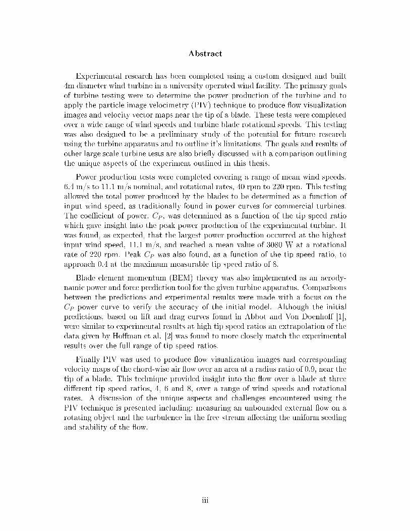
AbstractExperimental research has been completed using a custom designed and built4m diameter wind turbine in a university operated wind facility. The primary goalsof turbine testing were to determine the power production of the turbine and toapply the particle image velocimetry (PIV) technique to produce ow visualizationimages and velocity vector maps near the tip of a blade. These tests were completedover a wide range of wind speeds and turbine blade rotational speeds. This testingwas also designed to be a preliminary study of the potential for future researchusing the turbine apparatus and to outline it's limitations. The goals and results ofother large scale turbine tests are also briey discussed with a comparison outliningthe unique aspects of the experiment outlined in this thesis.Power production tests were completed covering a range of mean wind speeds,6.4 m/s to 11.1 m/s nominal, and rotational rates, 40 rpm to 220 rpm. This testingallowed the total power produced by the blades to be determined as a function ofinput wind speed, as traditionally found in power curves for commercial turbines.The coecient of power, CP , was determined as a function of the tip speed ratiowhich gave insight into the peak power production of the experimental turbine. Itwas found, as expected, that the largest power production occurred at the highestinput wind speed, 11.1 m/s, and reached a mean value of 3080 W at a rotationalrate of 220 rpm. Peak CP was also found, as a function of the tip speed ratio, toapproach 0.4 at the maximum measurable tip speed ratio of 8.Blade element momentum (BEM) theory was also implemented as an aerody-namic power and force prediction tool for the given turbine apparatus. Comparisonsbetween the predictions and experimental results were made with a focus on theCP power curve to verify the accuracy of the initial model. Although the initialpredictions, based on lift and drag curves found in Abbot and Von Doenho [1],were similar to experimental results at high tip speed ratios an extrapolation of thedata given by Homan et al. [2] was found to more closely match the experimentalresults over the full range of tip speed ratios.Finally PIV was used to produce ow visualization images and correspondingvelocity maps of the chord-wise air ow over an area at a radius ratio of 0.9, near thetip of a blade. This technique provided insight into the ow over a blade at threedierent tip speed ratios, 4, 6 and 8, over a range of wind speeds and rotationalrates. A discussion of the unique aspects and challenges encountered using thePIV technique is presented including: measuring an unbounded external ow on arotating object and the turbulence in the free stream aecting the uniform seedingand stability of the ow.

iii

AcknowledgmentsMany people have helped me with the content that has gone into this the-sis or during the writing phase. From design work to time in the machine shop;troubleshooting experiments to grunt work moving bricks, everyone in the researchgroup had a hand in this project and I appreciate all of their help.I would rst like to thank my supervisor Dr. David Johnson who's guidancethroughout my degree has been instrumental in getting me to this point. Whetherit was related to my degree or not he was there to provide words of encouragementand excellent advice.To everybody in the research group you have all helped to make this possible innumerous ways. First to Ammar Altaf and Zeyad Almutairi who made me feel sowelcome when I rst arrived at the University. Ammar also helped me immenselyto learn how to operate the PIV equipment. Stephen Orlando, Erik Skensvedand Curtis Knischewsky for putting in a lot of time and eort in the design andconstruction of various components of the turbine rig and with it's installation.Kobra Gharali for her in-depth knowledge of PIV image processing. Adam Bale,Drew Gertz and Vivian Lam for their additional help through the testing phaseof this project. Adam McPhee as someone to bounce ideas o of throughout mydegree. Finally to Michael McWilliam for designing the turbine apparatus andtower and putting in many hours in the machine shop to make parts.To my friends Neil Norris and Andrew Berg for letting me crash on their couchin the nal weeks of my experiments (note to others: nish your experiments beforegiving your landlord 60 days notice).The support sta and technicians in the department that have helped to makethis project come together. I would specically like to thank Gord Hitchman forhis help at the wind facility while running the experiments and Andy Barber andJim Merli for their electrical support. Also Ed Spike for his help in getting thenecessary equipment to run the electrical side of the experiments. John Potzoldwas also very helpful in teaching me to use the equipment in the machine shop.Composotech Structures Inc. for completing the turbine blades and for walkingme through the manufacturing process on-site and Chris Wraith for his follow-upcorrespondence.Most of all, I would like to give a special thanks to my mom who has been verysupportive of me throughout my undergraduate and graduate degrees and mostrecently during the writing of my thesis. Pushing me forward when I needed a bitof a nudge and knowing when I needed to clear my head. I don't know how I wouldhave completed this without your support.iv

DedicationI would like to dedicate this thesis to the memory of my dad, David GeorgeGaunt. He was instrumental in guiding me towards a career in engineering and Ilikely wouldn't be here without his support and encouragement which helped pushme to succeed. I know how proud you would be to see this accomplishment.

v

ContentsList of Tables xiList of Figures xvNomenclature xviii1 Introduction 11.1 Wind Energy . . . . . . . . . . . . . . . . . . . . . . . . . . . . . . 11.2 Goals and Objectives . . . . . . . . . . . . . . . . . . . . . . . . . . 22 Background and Theory 42.1 Previous Large Scale Wind Turbine Tests . . . . . . . . . . . . . . . 42.1.1 NREL . . . . . . . . . . . . . . . . . . . . . . . . . . . . . . 42.1.2 MEXICO . . . . . . . . . . . . . . . . . . . . . . . . . . . . 92.2 BEM Theory and Implementation . . . . . . . . . . . . . . . . . . . 132.2.1 Overview . . . . . . . . . . . . . . . . . . . . . . . . . . . . 132.2.2 Assumptions . . . . . . . . . . . . . . . . . . . . . . . . . . . 132.2.3 Procedure Overview . . . . . . . . . . . . . . . . . . . . . . 132.2.4 BEM Implementation . . . . . . . . . . . . . . . . . . . . . . 142.2.5 Force and Power Determination . . . . . . . . . . . . . . . . 162.3 Particle Image Velocimetry . . . . . . . . . . . . . . . . . . . . . . . 182.3.1 PIV Theory . . . . . . . . . . . . . . . . . . . . . . . . . . . 182.3.2 Application of PIV to rotating objects . . . . . . . . . . . . 19

vi

3 Experimental Equipment 213.1 Equipment overview . . . . . . . . . . . . . . . . . . . . . . . . . . 213.2 Wind Facility . . . . . . . . . . . . . . . . . . . . . . . . . . . . . . 213.2.1 Wind Velocity Characteristics . . . . . . . . . . . . . . . . . 233.2.2 Fan Frequency to Velocity Correlation . . . . . . . . . . . . 233.2.3 Turbulence Intensity . . . . . . . . . . . . . . . . . . . . . . 243.3 Turbine Assembly . . . . . . . . . . . . . . . . . . . . . . . . . . . . 243.3.1 Modications . . . . . . . . . . . . . . . . . . . . . . . . . . 253.4 Turbine Blades . . . . . . . . . . . . . . . . . . . . . . . . . . . . . 303.5 Blade Geometry . . . . . . . . . . . . . . . . . . . . . . . . . . . . . 313.5.1 Chord and Twist Measurements . . . . . . . . . . . . . . . . 313.5.2 Airfoil Distribution . . . . . . . . . . . . . . . . . . . . . . . 323.6 Airfoil Aerodynamic Properties . . . . . . . . . . . . . . . . . . . . 343.6.1 Lift and Drag Extrapolation . . . . . . . . . . . . . . . . . . 363.6.2 Lift and Drag Data sets . . . . . . . . . . . . . . . . . . . . 373.7 PIV Equipment . . . . . . . . . . . . . . . . . . . . . . . . . . . . . 413.7.1 Control . . . . . . . . . . . . . . . . . . . . . . . . . . . . . 413.7.2 Camera . . . . . . . . . . . . . . . . . . . . . . . . . . . . . 423.7.3 Laser . . . . . . . . . . . . . . . . . . . . . . . . . . . . . . . 423.7.4 Seeding . . . . . . . . . . . . . . . . . . . . . . . . . . . . . 433.8 Power Supply and Loading of the Motor/Generator . . . . . . . . . 443.8.1 Overview . . . . . . . . . . . . . . . . . . . . . . . . . . . . 443.8.2 Motor Power Supply . . . . . . . . . . . . . . . . . . . . . . 453.8.3 Generator Loading . . . . . . . . . . . . . . . . . . . . . . . 463.8.4 Wiring Box . . . . . . . . . . . . . . . . . . . . . . . . . . . 463.9 Instrumentation . . . . . . . . . . . . . . . . . . . . . . . . . . . . . 483.9.1 Data Acquisition Hardware . . . . . . . . . . . . . . . . . . 483.9.2 Tunnel Velocity Measurements . . . . . . . . . . . . . . . . . 483.9.3 Rotational Speed . . . . . . . . . . . . . . . . . . . . . . . . 483.9.4 Voltage, Current and Power . . . . . . . . . . . . . . . . . . 493.9.5 Labview [45] . . . . . . . . . . . . . . . . . . . . . . . . . . . 50vii

4 Experimental Procedure 524.1 Performance Measurements . . . . . . . . . . . . . . . . . . . . . . 524.1.1 Drivetrain Loss Estimation . . . . . . . . . . . . . . . . . . . 524.1.2 Power Production . . . . . . . . . . . . . . . . . . . . . . . . 534.2 Experimental PIV Procedure . . . . . . . . . . . . . . . . . . . . . 554.2.1 Area of Interest . . . . . . . . . . . . . . . . . . . . . . . . . 554.2.2 Focus and Alignment . . . . . . . . . . . . . . . . . . . . . . 564.2.3 Seeding . . . . . . . . . . . . . . . . . . . . . . . . . . . . . 574.2.4 Trigger Timing . . . . . . . . . . . . . . . . . . . . . . . . . 574.2.5 Interframe Rate . . . . . . . . . . . . . . . . . . . . . . . . . 604.2.6 Image Correlation . . . . . . . . . . . . . . . . . . . . . . . . 604.3 PIV Post-Processing Technique . . . . . . . . . . . . . . . . . . . . 624.3.1 Concept . . . . . . . . . . . . . . . . . . . . . . . . . . . . . 624.3.2 Image Shift Program Verication . . . . . . . . . . . . . . . 654.3.3 Experimental Image Processing . . . . . . . . . . . . . . . . 654.4 Test Case Selection . . . . . . . . . . . . . . . . . . . . . . . . . . . 664.4.1 Performance Testing . . . . . . . . . . . . . . . . . . . . . . 704.4.2 PIV Testing . . . . . . . . . . . . . . . . . . . . . . . . . . . 705 Results 715.1 Experimental Performance . . . . . . . . . . . . . . . . . . . . . . . 715.1.1 Outliers . . . . . . . . . . . . . . . . . . . . . . . . . . . . . 715.1.2 Power Losses . . . . . . . . . . . . . . . . . . . . . . . . . . 725.1.3 Power Generation . . . . . . . . . . . . . . . . . . . . . . . . 755.1.4 CP vs TSR . . . . . . . . . . . . . . . . . . . . . . . . . . . 755.2 BEM Results . . . . . . . . . . . . . . . . . . . . . . . . . . . . . . 775.2.1 Eect of the number of elements . . . . . . . . . . . . . . . . 785.2.2 Axial Induction Convergence Study . . . . . . . . . . . . . . 785.2.3 Eects of Tip losses . . . . . . . . . . . . . . . . . . . . . . . 795.2.4 Program Output . . . . . . . . . . . . . . . . . . . . . . . . 805.2.5 Experimental and BEM CP Comparison . . . . . . . . . . . 855.2.6 Summary of Experimental Power Production and BEM Mod-eling . . . . . . . . . . . . . . . . . . . . . . . . . . . . . . . 86viii

5.3 PIV Results . . . . . . . . . . . . . . . . . . . . . . . . . . . . . . . 875.3.1 Averaged Flow Results . . . . . . . . . . . . . . . . . . . . . 875.3.2 Variance in Averaged PIV Results . . . . . . . . . . . . . . . 885.3.3 Relative Frame of Reference . . . . . . . . . . . . . . . . . . 935.3.4 Repeatability . . . . . . . . . . . . . . . . . . . . . . . . . . 945.3.5 Summary of PIV Results . . . . . . . . . . . . . . . . . . . . 996 Conclusions 1016.1 Wind Turbine Power Production . . . . . . . . . . . . . . . . . . . 1016.2 BEM Predictions . . . . . . . . . . . . . . . . . . . . . . . . . . . . 1016.3 PIV . . . . . . . . . . . . . . . . . . . . . . . . . . . . . . . . . . . 1026.4 Equipment Improvements . . . . . . . . . . . . . . . . . . . . . . . 1026.4.1 Turbine and Blade Assembly . . . . . . . . . . . . . . . . . . 1036.4.2 Wind Facility . . . . . . . . . . . . . . . . . . . . . . . . . . 1036.4.3 Instrumentation . . . . . . . . . . . . . . . . . . . . . . . . . 1046.4.4 PIV Equipment . . . . . . . . . . . . . . . . . . . . . . . . . 1046.5 Recommendations for Future Research Projects . . . . . . . . . . . 1056.5.1 Power Production Studies . . . . . . . . . . . . . . . . . . . 1056.5.2 BEM Model Studies . . . . . . . . . . . . . . . . . . . . . . 1056.5.3 PIV Studies . . . . . . . . . . . . . . . . . . . . . . . . . . . 106References 107Appendices 111A BEM 111A.1 Betz Limit Derivation . . . . . . . . . . . . . . . . . . . . . . . . . 111A.2 BEM Matlab Code . . . . . . . . . . . . . . . . . . . . . . . . . . . 113B Error Analysis 116B.1 Velocity Error . . . . . . . . . . . . . . . . . . . . . . . . . . . . . . 116B.2 Error in power calculations . . . . . . . . . . . . . . . . . . . . . . . 117B.3 Error in coecient of power calculations . . . . . . . . . . . . . . . 119C Installation and Decommissioning of the Wind Turbine 121ix

D Turbine Blade Fabrication 124D.1 Mould and Material Preparation . . . . . . . . . . . . . . . . . . . . 124D.2 Process . . . . . . . . . . . . . . . . . . . . . . . . . . . . . . . . . . 126D.3 Fibreglass Lamination Schedule . . . . . . . . . . . . . . . . . . . . 127D.4 Skin Layer . . . . . . . . . . . . . . . . . . . . . . . . . . . . . . . . 129D.4.1 Second Lamination - triax . . . . . . . . . . . . . . . . . . . 129D.4.2 Third and Fourth Lamination - triax . . . . . . . . . . . . . 129D.4.3 Fifth to Seventh Lamination - UD . . . . . . . . . . . . . . . 130D.4.4 Texture mat . . . . . . . . . . . . . . . . . . . . . . . . . . . 130D.5 Spar . . . . . . . . . . . . . . . . . . . . . . . . . . . . . . . . . . . 132D.6 Mating Moulds . . . . . . . . . . . . . . . . . . . . . . . . . . . . . 132E PIV Smoke Injection Methods 134F Post Processing Code 137F.1 Image Shift Determination . . . . . . . . . . . . . . . . . . . . . . . 137F.2 PIV results Shift . . . . . . . . . . . . . . . . . . . . . . . . . . . . 138F.3 Image Shifting . . . . . . . . . . . . . . . . . . . . . . . . . . . . . . 139

x

List of Tables2.1 Turbine and tunnel conditions varied during NREL testing [5] . . . 52.2 Turbine and tunnel conditions varied during MEXICO testing [6] . 103.1 Turbulence intensity over a range of fan settings . . . . . . . . . . . 253.2 Aerodynamic property data sets used for BEM calculations with orig-inal data parameters and the method used for data extrapolation . 354.1 Signal Generator settings for PIV . . . . . . . . . . . . . . . . . . . 594.2 Theoretical and experimental interframe rates . . . . . . . . . . . . 604.3 Comparison of manual shift determination and Matlab [17] imageshift program . . . . . . . . . . . . . . . . . . . . . . . . . . . . . . 664.4 Five test cases used in PIV experimentation . . . . . . . . . . . . . 705.1 Power loss data based on curve ts on the raw data . . . . . . . . . 745.2 Eect of increasing the number of elements . . . . . . . . . . . . . . 785.3 Convergence study . . . . . . . . . . . . . . . . . . . . . . . . . . . 79B.1 Accuracy error in the Keithley 2700 multimeter [42] . . . . . . . . . 118

xi

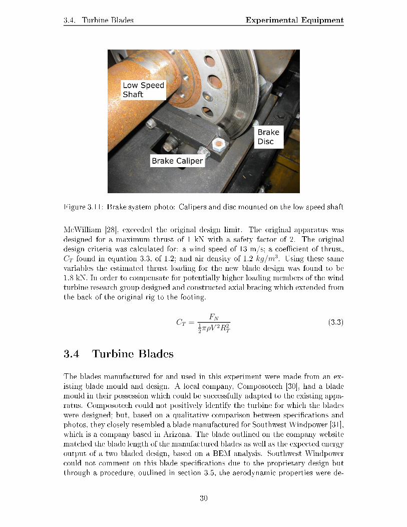
List of Figures1.1 Example of a modern turbine with major components labeled . . . 22.1 NREL UAE turbine in the NASA Ames wind tunnel [8] . . . . . . . 62.2 Sample surface pressure distribution from a point 30% from the bladeroot on the UAE turbine as presented by Schepers and Rooji [9] . . 72.3 MEXICO turbine in the German-Dutch wind tunnel [6] . . . . . . . 102.4 Sample of the induction measurements based on the MEXICO PIVdata [15] . . . . . . . . . . . . . . . . . . . . . . . . . . . . . . . . . 122.5 Velocity triangle for a rotating airfoil . . . . . . . . . . . . . . . . . 142.6 Blade force geometry . . . . . . . . . . . . . . . . . . . . . . . . . . 172.7 Schematic of PIV experimental setup and processing [24] . . . . . . 193.1 Overall experimental setup: plan view . . . . . . . . . . . . . . . . 223.2 Fan exit looking from downstream . . . . . . . . . . . . . . . . . . . 223.3 Sample velocity data at a fan setting of 60 Hz measured using thesonic anemometer, with single sample error shown, mean velocity of11 m/s . . . . . . . . . . . . . . . . . . . . . . . . . . . . . . . . . . 233.4 Relationship between fan frequency and streamwise velocity . . . . 243.5 Turbine assembly CAD model: prole view [28] . . . . . . . . . . . 263.6 Turbine assembly photo: Angled view with load bank, camera andlaser system in place . . . . . . . . . . . . . . . . . . . . . . . . . . 273.7 Turbine assembly photo: Prole view of nacelle . . . . . . . . . . . 273.8 Exploded view of mounting plates . . . . . . . . . . . . . . . . . . . 283.9 Brake system schematic . . . . . . . . . . . . . . . . . . . . . . . . 293.10 Brake system photo: Air cylinder and master brake cylinder . . . . 293.11 Brake system photo: Calipers and disc mounted on the low speedshaft . . . . . . . . . . . . . . . . . . . . . . . . . . . . . . . . . . . 303.12 Measured chord distribution of the manufactured turbine blades . . 31xii

3.13 Twist distribution of the manufactured turbine blades . . . . . . . . 323.14 Mould casings in place along a nished blade at the root, mid-sectionand tip . . . . . . . . . . . . . . . . . . . . . . . . . . . . . . . . . . 333.15 Tip mould casing removed from blade and cut at midpoint . . . . . 333.16 Measured blade coordinates compared with NACA proles: a) thetip, b) middle and c) root . . . . . . . . . . . . . . . . . . . . . . . 343.17 Coecient of drag as a function of the coecient of lift [1] . . . . . 373.18 Lift coecient as a function of α [1, 2, 34, 35] . . . . . . . . . . . . 393.19 Drag coecient as a function of α [1, 2, 34, 35] . . . . . . . . . . . . 403.20 Lift coecient comparison between raw data and the Viterna ex-trapolation [34] . . . . . . . . . . . . . . . . . . . . . . . . . . . . . 403.21 Drag coecient comparison between raw data and the AirfoilPrepextrapolations [34] . . . . . . . . . . . . . . . . . . . . . . . . . . . 413.22 Final seeding method smoke generator and condensate collector . . 433.23 Final seeding method . . . . . . . . . . . . . . . . . . . . . . . . . . 443.24 Electrical system wiring schematic . . . . . . . . . . . . . . . . . . . 453.25 Load bank schematic . . . . . . . . . . . . . . . . . . . . . . . . . . 473.26 Sonic anemometer placed in tunnel air ow . . . . . . . . . . . . . . 493.27 Power generation schematic . . . . . . . . . . . . . . . . . . . . . . 503.28 Motoring schematic . . . . . . . . . . . . . . . . . . . . . . . . . . . 514.1 Raw power curve for data collected at U∞ =3.5 m/s (above) andU∞ = 6.4 m/s, demonstrating high levels of variability at low velocities 544.2 Calibration image, with a ruler in the frame, used to focus the cameraand determine image scale . . . . . . . . . . . . . . . . . . . . . . . 564.3 Pulse schematic . . . . . . . . . . . . . . . . . . . . . . . . . . . . . 584.4 Signal Generator settings for PIV . . . . . . . . . . . . . . . . . . . 594.5 Sample correlation surface plot . . . . . . . . . . . . . . . . . . . . 614.6 Master image used to determine the shift vector for each raw imagepair . . . . . . . . . . . . . . . . . . . . . . . . . . . . . . . . . . . 624.7 Shift vector concept . . . . . . . . . . . . . . . . . . . . . . . . . . . 634.8 Common area found after determining the shift vector for all imageswithin a test case . . . . . . . . . . . . . . . . . . . . . . . . . . . . 644.9 Shifted image, before (left) and after (right) . . . . . . . . . . . . . 644.10 Raw images used in PIV analysis with the well seeded image shownabove, TSR 3.8, Ω = 198RPM, U∞ = 11.8m/s . . . . . . . . . . . . 67xiii

4.11 Contour plots showing accepted vectors in blue for each of the rawimage correlations, TSR 3.8, Ω = 198 RPM, U∞ = 11.8m/s (wellseeded above) . . . . . . . . . . . . . . . . . . . . . . . . . . . . . . 684.12 Vector plots from individual image pairs, TSR 3.8, Ω = 198 RPM,U∞ = 11.8m/s (well seeded above) . . . . . . . . . . . . . . . . . . . 695.1 Overall power loss data . . . . . . . . . . . . . . . . . . . . . . . . . 735.2 Dierence between power measured with and without the bladesattached as a function of the rotational speed . . . . . . . . . . . . 745.3 Power generated by the blades . . . . . . . . . . . . . . . . . . . . . 765.4 Power at the blades with varying wind speed, Ω= 220 rpm . . . . . 765.5 Raw experimental CP results . . . . . . . . . . . . . . . . . . . . . . 775.6 The eect of the number of elements used in the BEM analysis onthe CP . . . . . . . . . . . . . . . . . . . . . . . . . . . . . . . . . . 795.7 Convergence criteria eect on the CP . . . . . . . . . . . . . . . . . 805.8 Tip loss factor along the length of the blade . . . . . . . . . . . . . 815.9 Eect of tip losses on the elemental power produced . . . . . . . . . 815.10 Eect of TSR on the AOA over a blade at a wind speed of 11 m/s . 825.11 Eect of the input β distribution on the AOA output . . . . . . . . 835.12 Eect of TSR on the axial induction factor, a . . . . . . . . . . . . 845.13 Eect of TSR on the tangential induction factor, a′ . . . . . . . . . 845.14 Eect of the Flat or Viterna extrapolation on the calculated CP withthe experimental results also shown . . . . . . . . . . . . . . . . . . 855.15 Two BEM results compared to experimental CP results found duringtesting . . . . . . . . . . . . . . . . . . . . . . . . . . . . . . . . . . 865.16 Absolute average vector map from unshifted PIV data, TSR 3.8,Ω = 198 RPM, U∞ = 11.8m/s . . . . . . . . . . . . . . . . . . . . . 885.17 Absolute average vector map from shifted PIV data, TSR 3.8, Ω =198 RPM, U∞ = 11.8m/s . . . . . . . . . . . . . . . . . . . . . . . . 895.18 Variability of the data in the unshifted PIV data set with σvel rep-resented by contours, TSR 3.8, Ω = 198 RPM, U∞ = 11.8m/s . . . 905.19 Variability of the data in the shifted PIV data set with σvel repre-sented by contours, TSR 3.8, Ω = 198 RPM, U∞ = 11.8m/s . . . . 915.20 Contour plot representing the number of vectors that comprised eachaveraged vector, TSR 3.8, Ω = 198 RPM, U∞ = 11.8m/s . . . . . . 925.21 Relative reference frame from shifted PIV data, TSR 3.7, Ω = 195RPM, U∞ = 11m/s . . . . . . . . . . . . . . . . . . . . . . . . . . . 93xiv

5.22 Contour plot representing AOA with streamlines representing theow over a blade, TSR 3.8, Ω = 198 RPM, U∞ = 11.8m/s . . . . . 955.23 Contour plot representing AOA with streamlines representing theow over blade, TSR 3.7, Ω = 111 RPM, U∞ = 6.8m/s . . . . . . . 965.24 Contour plot representing AOA with streamlines representing theow over a blade, TSR 7.4, Ω = 220 RPM, U∞ = 6.8m/s . . . . . . 975.25 Comparison of two tests under the same conditions on separate daysat a nominal TSR of 3.8, Ω = 198 RPM, U∞ = 11.8m/s . . . . . . . 985.26 Comparison of a common data set with dierent sample sizes, TSR3.8, Ω = 198 RPM, U∞ = 11.8 m/s . . . . . . . . . . . . . . . . . . 99A.1 Rotor model used in the BEM analysis [16] . . . . . . . . . . . . . . 112B.1 Free stream velocity with both single measurement and mean errorshown for comparison . . . . . . . . . . . . . . . . . . . . . . . . . . 117C.1 Raising of the nacelle to the mounting point on top of the tower(Side view) . . . . . . . . . . . . . . . . . . . . . . . . . . . . . . . 122C.2 Raising of the nacelle to the mounting point on top of the tower(Front view) . . . . . . . . . . . . . . . . . . . . . . . . . . . . . . . 123D.1 Two piece mould prior to material lay-up, bottom half is on the right 125D.2 Lamination schedule drawing with key positions labeled . . . . . . . 125D.3 Gel coat being applied to the lower mould . . . . . . . . . . . . . . 126D.4 Areas of the mould which required putty to ll small radius areas . 127D.5 Bubbles under the skin layer at the edge of the blade mould cavity . 128D.6 Cutaway view of the blade structure . . . . . . . . . . . . . . . . . 128D.7 Skin layer cuts made to avoid wrinkles in bottom half of the mould 129D.8 Triax trimmed to be 1 cm from the mould edge at the tip . . . . . . 130D.9 Mould with the fourth lamination applied . . . . . . . . . . . . . . 131D.10 UD layer application . . . . . . . . . . . . . . . . . . . . . . . . . . 131D.11 Textured mat application . . . . . . . . . . . . . . . . . . . . . . . . 132E.1 Failed smoke method with smoke generator placed on the condition-ing grid . . . . . . . . . . . . . . . . . . . . . . . . . . . . . . . . . 135E.2 Failed smoke method using a manifold with ow straightening tubesto aid in mixing and smoke stream quality . . . . . . . . . . . . . . 136xv

NomenclatureRoman Symbolsa Axial induction factor (-)a′ Tangential induction factor (-)AR Aspect ratio of the turbine blade (-)C Chord length of the airfoil (m)CD Coecient of drag (-)CDflat Coecient of drag based on at plate theory (-)CDmax Maximum coecient of drag (-)CL Coecient of lift (-)CP Coecient of power (-)CT Coecient of Thrust (-)dA Dierential blade area (m2)dD Dierential blade drag (N)dFN Dierential normal blade force (N)dFT Dierential tangential blade force (N)dL Dierential blade lift force (N)dP Dierential blade power (W)dR Dierential blade radius (m)dT Dierential torque (Nm)F Tip loss factor (-)ffan Fan frequency (Hz) xvi

G Gain in shunt resistor (A/V)Iarm Current at the armature (A)I Current (A)IS Shunt current (A)IT Free stream turbulence intensity (-)N Number of blades (-)NS Number of Samples (-)PAero Power loss due to aerodynamic drag (W)PBlade Power generated by blades (W)PDrive Power loss due to the drive train (W)PGEN Power in or out of generator (W)PGrid Power input at the motor (W)PLoad Power input at the load bank (W)R Resistance (Ω)r Radial location along blade (m)RT Tip radius (m)tmax Maximum theoretical interframe rate (s)Tmotor Torque output by motor (Nm)tS T-value from two tailed Student's t-distribution (-)U∞ Freestream velocity (m/s)U∞ Mean of the streamwise velocity (m/s)Vabs Absolute velocity (m/s)Varm Voltage at the armature (V)VS Shunt Voltage (V)V Voltage (V)Vy Velocity tangential (y-direction) to the blades rotation (m/s)W Relative velocity (m/s) xvii

X Number of interrogation areas in the x-direction (-)Y Number of interrogation areas in the y-direction (-)Greek Symbolsα Angle of attack (deg)αref Maximum angle of attack within a data set (deg)β Blade set angle (deg)∆G Error in gain value (A/V)∆I Error in current measurement (A)∆P Error in measured power (W)∆V Error in the voltage measurement (V)λT Tip speed ratio (-)λr Local speed ratio (-)Ω Blade rotational speed (rpm)ωmotor Rotational speed of the motor (rad/s)φ Inow angle (deg)Φ Magnetic ux generated by eld windings (Wb)ρ Density (kg/m3)σ Chord solidity (-)σS Standard deviation of a data set (-)σU Standard deviation of U velocity vector (m/s)σU∞

Standard deviation of the streamwise velocity (m/s)σV Standard deviation of V velocity vector (m/s)σvel Standard deviation of PIV velocity vectors (m/s)

xviii

Such experiments are frequently congured like icebergs: Only about 10% ofthe eort shows as output data; the other 90% which establishes the validity of the10%, is unseen - relegated to the logbook.Robert J. Moat, Describing the Uncertainties in Experimental Results

xix

Chapter 1Introduction1.1 Wind EnergyWith a current social and economic drive to develop alternative energy sources theextraction of power, using wind turbines, from renewable wind resources around theworld represents an alternative to current non-renewable power sources. Worldwide,wind turbine power capacity was increased by 26% in 2007 over the capacity in 2006.This increased capacity represented a nameplate power increase of approximately 13GW [3]. Canadian 2008 energy statistics [4] indicated that Canadian wind turbinesproduce 1.7 TWh of energy which represents 0.29% of the total Canadian utilityenergy production. In contrast, Denmark has 1.7 times the installed wind turbinecapacity of Canada but the energy these turbines produce accounts for 19.9% oftheir energy production [3]. Although this comparison does not account for therespective populations of the countries it does represent the level at which windenergy can become a part of a country's energy mix.Despite the continuing growth of the wind energy industry improvements to thedesign and operation of turbines are always possible. Experimental studies of windturbine aerodynamics have the potential to improve the operation and eciencyof turbines and the initial prediction of their output. These improvements canultimately aid in the adoption of these products and help to increase their part inthe world's energy mix.Modern grid connected wind turbines are predominately three-bladed horizontal-axis machines. While the internal design varies between manufacturers a basic tur-bine consists of four major parts: the blades, hub, nacelle and tower. The bladesare typically made of a breglass composite structure and range in length depend-ing on the designed power rating of the turbine. The blades are the componentwhich extracts the energy from the wind and transfers it into rotational motion.The hub is the component which connects the blades to the nacelle and, dependingon the design, can incorporate active blade pitch control. The nacelle contains allof the mechanical components which, depending on the design, can include: a gear1

1.2. Goals and Objectives Introductionbox, generator, braking system and yaw control. Finally, the tower is the structurewhich supports the nacelle, hub and blades and is typically mounted on a rein-forced concrete base. A typical modern turbine is shown below in gure 1.1 withthe major components labeled and a person standing approximately 50 m from thebase for reference.

Figure 1.1: Example of a modern turbine with major components labeled1.2 Goals and ObjectivesThe goal of this project was to gain a better understanding of the unique charac-teristics of wind turbine aerodynamics through experimentation. Specically thisexperimentation was completed on a rotating large scale 4.3 m diameter wind tur-bine in a University operated wind facility. This project was broken up into threedistinct, but related, areas of study: i) the completion of an experimental studywhich determined the power generation of a wind turbine over a range of rotational2

1.2. Goals and Objectives Introductionrates and wind speeds; ii) the development of a numerical, momentum based, modelwhich was used to predict turbine blade loading and power generation; and iii) proofof concept experimental ow measurements around a turbine blade using a laserbased velocity measurement technique. For organizational purposes each area ofstudy is presented in separate sections within each relevant chapter. In addition tothe major areas of study, a discussion of improvements which can be made to thewind turbine apparatus and wind facility and recommendations for further studieswas made.For the experimental portions of this project a wind turbine apparatus, designedto test various turbine blade congurations, was commissioned for use in a Univer-sity operated wind facility. The commissioning process involved nal assembly ofvarious components of the apparatus as well as it's instrumentation. Ultimately oneset of turbine blades was tested on this apparatus and the power they produced atvarying wind speeds and rotational rates was quantied. The ow close to the tipof a rotating blade was also visualized and quantied using a laser based technique.

3

Chapter 2Background and TheoryThis chapter will present a brief background and discuss the theory related to thework completed for this thesis. The rst topic includes a discussion of previous largescale wind turbine experimentation which includes an outline of: the experimentalequipment used, the results of the testing and the contribution the testing madeto further wind turbine research. Secondly, there is a discussion of the momentumbased model which was used to predict the output of the wind turbine tested inthis experiment. Finally, there is an introduction to the laser based method usedto quantify the blade ow near the tip and a discussion of the unique aspects of it'sapplication in this experiment.2.1 Previous Large Scale Wind Turbine TestsDue to the scale of commercial wind turbines, with rotor diameters on the orderof 100 m, testing of scale models under controlled conditions, like those found ina wind tunnel, has been limited to a very small number of experiments. Twomajor projects that have been completed will be discussed in this section: the rstcompleted by the National Renewable Energy Laboratory (NREL) in the NationalFull-Scale Aerodynamics Complex at NASA's Ames research facility [5]; and thesecond project, MEXICO, was coordinated by the Energy Research Center of theNetherlands (ECN) with tests completed at the large scale low speed wind tunnel(LLF) which is part of the German-Dutch Wind tunnel (DNW) network [6]. Whilethe goals and objectives of these two tests were not identical they represent theforemost large scale wind tunnel testing of wind turbines to date.2.1.1 NRELBased on testing by NREL in the NASA Ames wind tunnel the research communitywas provided with experimental data which covered blade pressure measurements4

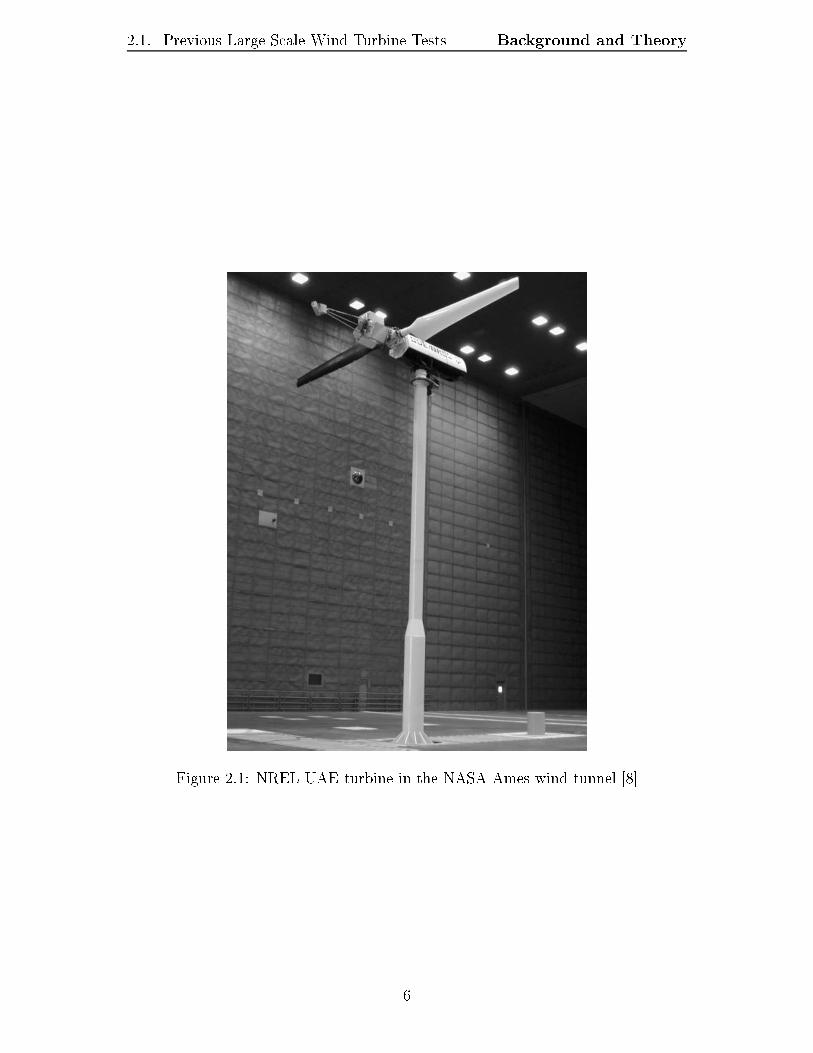
2.1. Previous Large Scale Wind Turbine Tests Background and TheoryTable 2.1: Turbine and tunnel conditions varied during NREL testing [5]Test Variable Range of ValuesWind Speed 5 to 39.3 m/sRotational Rate 0, 72, 90 rpmBlade Pitch 3 to 79 degreesYaw Angle -180 to 180 degreesCone Angle 0, 3.4, 18 degreesand power production data with which to compare predictive models. The windfacility used and the turbine tested are briey described below.Research that has been completed based on the results of this testing are alsodiscussed with a focus on three dimensional ow eects and the improvement ofnumerical models used to predict turbine power and loading. These two topics wererelevant to the research completed for this thesis due to the power prediction thatwas completed and the eect that the three dimensional eects could have on thePIV measurements.Overall 30 dierent tests were completed utilizing dierent turbine congura-tions which varied: the wind input speeds, yaw angle, blade tip design, upwindor downwind rotor, three rotational rates, pitch angle, teetering or rigid hub andnally coning of the rotor. A brief summary of the turbine and tunnel conditionsused during the NREL testing outlined in table 2.1.2.1.1.1 Turbine and Tunnel overviewCompleted in 2000, testing of the NREL unsteady aerodynamics experiment (UAE)wind turbine, in NASA's 24.4 m by 36.6 m wind tunnel, provided the wind turbineresearch community with information on the ow and power characteristics of awind turbine under controlled wind conditions. Prior to this testing informationon UAE turbine performance had been gathered in outdoor conditions where winddirection, wind speed and turbulence could not be controlled. The turbine testedwas a two bladed constant rotational rate, primarily 72 rpm, stall regulated designwith a 10 m rotor diameter and a rated power of 20 kW. The turbine blades usedthe S809 airfoil along the entire span with the airfoil designed and tested by Somers[7] for NREL. The majority of physical parameters of the turbine and wind tunneland test conditions relevant to the NREL testing are contained in a report producedby Hand et al. [5]. Figure 2.1 depicts the NREL UAE wind turbine installed in thewind tunnel.2.1.1.2 InstrumentationIn addition to instrumentation monitoring wind tunnel conditions, such as atmo-spheric pressure and wind speed, the turbine was instrumented to measure blade5

2.1. Previous Large Scale Wind Turbine Tests Background and Theory

Figure 2.1: NREL UAE turbine in the NASA Ames wind tunnel [8]

6

2.1. Previous Large Scale Wind Turbine Tests Background and Theory

Figure 2.2: Sample surface pressure distribution from a point 30% from the bladeroot on the UAE turbine as presented by Schepers and Rooji [9]ow characteristics as well as turbine loading and power production as describedby Hand et al. [5]. Specically a blade was outtted with surface mounted pressuretaps, aligned chord-wise, at ve radial locations, along the blade. These surfacemounted taps would provide pressure distribution data, and thus loading, alongthe blade. A sample pressure distribution, shown in gure 2.2 was presented bySchepers and Rooji [9] in a comparison to CFD output and was produced using thesurface pressure measurements.Five hole probes were also mounted to a blade which could measure pressureahead of the leading edge to provide information on the dynamic pressure andinow angles at ve radial locations. Strain gauges were also mounted to eachblade root in order to measure bending moments on the blades. Finally, the towerwas mounted to a load balance to measure the forces and moments applied to theentire apparatus. It should be noted that the instrumentation implemented in theNREL testing could not quantify the velocity eld around the blades.2.1.1.3 Three Dimensional Flow and Performance PredictionA common use of the NREL test results were for the comparison and validationof numerical models which attempted to quantify three dimensional eects on arotating turbine blade. These comparisons were typically used to gain a betterunderstanding of the complex ow over a wind turbine blade which can ultimatelyimprove power and load prediction for design purposes. Based on past and currentwork it was found that models still have diculty consistently predicting poweroutput and blade loading on turbines and as such cannot be the only tool used fordesign purposes. 7

2.1. Previous Large Scale Wind Turbine Tests Background and TheoryOne of NREL's goals was to determine the ecacy of models in predicting thepower output of the the UAE turbine when the researchers had no prior knowledgeof the UAE experimental results. This was called the aerodynamics code blindcomparison, discussed by Simms et al. [10], and involved many researchers with19 models ultimately implemented in an attempt to predict turbine loading andoutput. Researchers were given the same set of input data such as two dimen-sional aerodynamic airfoil properties and tunnel conditions at 20 operating pointsbut all experimental output results were unknown to researchers. The goal of thisproject was to determine not only the prediction uncertainty but also the aectthat the assumptions made by the researchers had on the accuracy of their model.Ultimately model predictions resulted in a wide range of results which never con-sistently matched experimental results. It was also found that some models couldpredict gross blade loading or power output at some test conditions but the span-wise power or loading distributions did not match experimental results.After the blind comparison study was complete, Coton et al. [11] attempted,among other goals, to determine the aect of aerodynamic property inputs on theaccuracy of model predictions against the NREL UAE data. It was found thatthe results did vary with dierent input aerodynamic properties which were theresult of two dimensional wind tunnel testing of the same S809 airfoil but underdierent Reynolds numbers or in dierent facilities. As only one model was used intheir study it was not possible to state with condence that inconsistent predictionswere the results of the model itself or of the input data but it was clear that threedimensional eects needed further study.Breton et al. [12], using the same model implemented by Coton et al. [11],attempted to determine the eect of various models used to correct two dimensionalaerodynamic airfoil data for three dimensional stall delay. It was found for thesemodels that corrections produced a wide range of predicted blade loading. It wassuggested that overprediction of lift near the tip was a dominant factor in poorprediction of experimental results as tip forces, due to their increased moment arm,have a larger power production potential.In an attempt to rule out the eect of aerodynamic properties of the airfoilon the accuracy of a model Laino et al. [13], as part of their study, determinedlift and drag properties based on measured inow angles and forces on the bladesduring the NREL tests. While this should provide the most accurate aerodynamicproperties for the prediction of blade loading the model did not accurately predictthe angle of attack that was measured by the probes mounted on a blade. As theangle of attack was not accurately predicted, the accuracy of the blade load pre-diction was not improved using this method. Further work was done to modify theaerodynamic properties for the model input to match the calculated experimen-tal force coecients. While this modied property input improved the accuracyof the model in both yawed and unyawed cases it ultimately required knowledgeof the experimental data to do so. However, three dimensional stall eects, in theyawed ow comparison, still aected the accuracy of the model which indicates thatmodeling these events still required improvements independent of the aerodynamic8

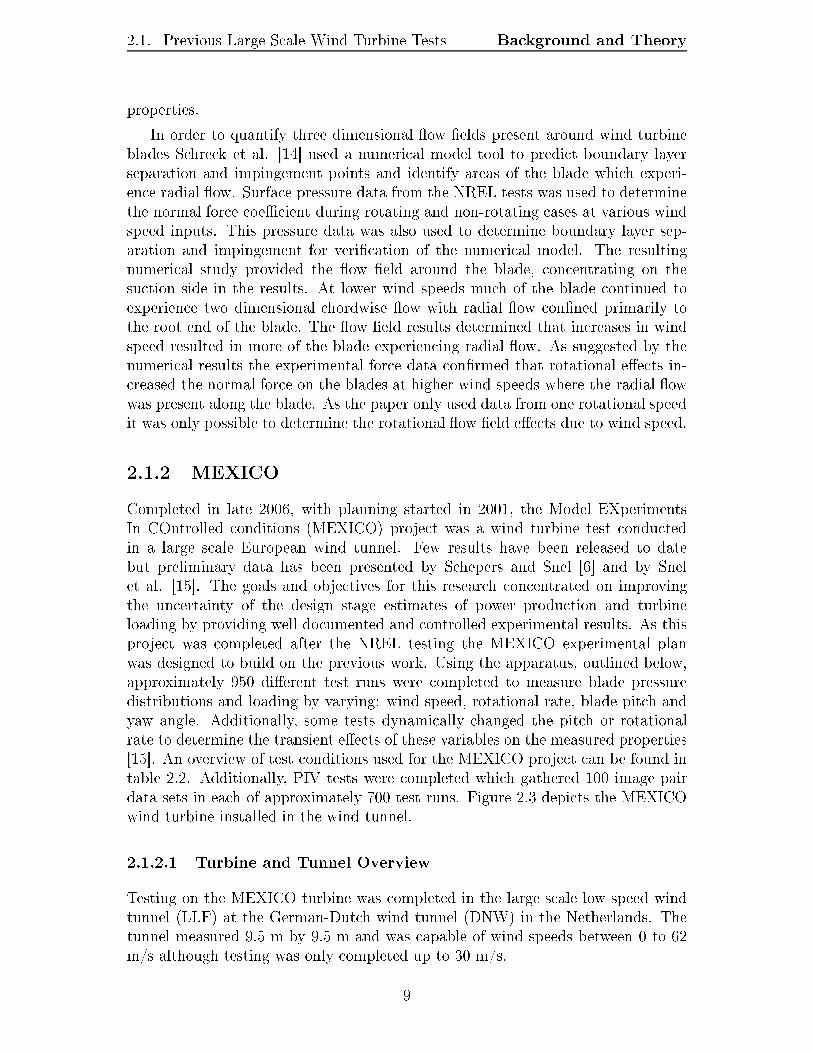
2.1. Previous Large Scale Wind Turbine Tests Background and Theoryproperties.In order to quantify three dimensional ow elds present around wind turbineblades Schreck et al. [14] used a numerical model tool to predict boundary layerseparation and impingement points and identify areas of the blade which experi-ence radial ow. Surface pressure data from the NREL tests was used to determinethe normal force coecient during rotating and non-rotating cases at various windspeed inputs. This pressure data was also used to determine boundary layer sep-aration and impingement for verication of the numerical model. The resultingnumerical study provided the ow eld around the blade, concentrating on thesuction side in the results. At lower wind speeds much of the blade continued toexperience two dimensional chordwise ow with radial ow conned primarily tothe root end of the blade. The ow eld results determined that increases in windspeed resulted in more of the blade experiencing radial ow. As suggested by thenumerical results the experimental force data conrmed that rotational eects in-creased the normal force on the blades at higher wind speeds where the radial owwas present along the blade. As the paper only used data from one rotational speedit was only possible to determine the rotational ow eld eects due to wind speed.2.1.2 MEXICOCompleted in late 2006, with planning started in 2001, the Model EXperimentsIn COntrolled conditions (MEXICO) project was a wind turbine test conductedin a large scale European wind tunnel. Few results have been released to datebut preliminary data has been presented by Schepers and Snel [6] and by Snelet al. [15]. The goals and objectives for this research concentrated on improvingthe uncertainty of the design stage estimates of power production and turbineloading by providing well documented and controlled experimental results. As thisproject was completed after the NREL testing the MEXICO experimental planwas designed to build on the previous work. Using the apparatus, outlined below,approximately 950 dierent test runs were completed to measure blade pressuredistributions and loading by varying: wind speed, rotational rate, blade pitch andyaw angle. Additionally, some tests dynamically changed the pitch or rotationalrate to determine the transient eects of these variables on the measured properties[15]. An overview of test conditions used for the MEXICO project can be found intable 2.2. Additionally, PIV tests were completed which gathered 100 image pairdata sets in each of approximately 700 test runs. Figure 2.3 depicts the MEXICOwind turbine installed in the wind tunnel.2.1.2.1 Turbine and Tunnel OverviewTesting on the MEXICO turbine was completed in the large scale low speed windtunnel (LLF) at the German-Dutch wind tunnel (DNW) in the Netherlands. Thetunnel measured 9.5 m by 9.5 m and was capable of wind speeds between 0 to 62m/s although testing was only completed up to 30 m/s.9

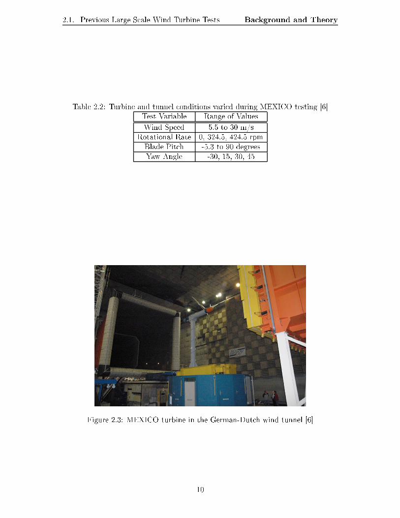
2.1. Previous Large Scale Wind Turbine Tests Background and TheoryTable 2.2: Turbine and tunnel conditions varied during MEXICO testing [6]Test Variable Range of ValuesWind Speed 5.5 to 30 m/sRotational Rate 0, 324.5, 424.5 rpmBlade Pitch -5.3 to 90 degreesYaw Angle -30, 15, 30, 45

Figure 2.3: MEXICO turbine in the German-Dutch wind tunnel [6]10

2.1. Previous Large Scale Wind Turbine Tests Background and TheoryThe wind turbine used for the MEXICO project was designed specically fortheir experiment and utilized a 4.5 m diameter three bladed rotor which was verysimilar in scale to the turbine apparatus used in the experimentation for this thesis.Although the rotational rate was not xed testing was only completed at threestates: 424.5 rpm, 324.5 rpm and parked. Additionally, the adjustable pitch bladeswere milled from aluminum to provide rigidity and repeatability between the blades.The prole of the blades varied along the radius and as such was a blend of threeseparate airfoils [6].2.1.2.2 InstrumentationIn order to expand on data gathered during the NREL tests pressure sensors wereplaced chordwise at ve radial locations. In all 148 sensors were used and dueto space constraints, within the blades, the sensors were spread amongst all threeblades with two blades measuring at two radial locations and the other blade atone radial location, although a small number of sensors were placed in at identicalpoints along each blade to ensure repeatability. Loads and bending moments werecalculated at the blades, using strain gauges, and at the base of the tower, using aload balance built into the wind tunnel.The signicant dierence from the NREL testing came from the MEXICOprojects PIV implementation. A three dimensional two camera PIV system wasused to measure ow: around the rotor plane, upstream and downstream of therotor plane, and near the blade tip to measure vortex structures. The PIV appa-ratus was able to move 10 m in the streamwise direction and 1.2 m radially alongthe blade. The area which could be measured by the PIV apparatus measured 337mm by 394 mm. The laser sheet used for these measurements was projected hori-zontally, in a plane parallel to the ground, from a point 270 degrees from vertical,in the clockwise direction.2.1.2.3 Preliminary MEXICO ResultsCurrent data from the MEXICO project is limited to preliminary results releasedby Snel et al. [15] and by Schepers and Snel [6]. The results presented by Snel etal. concentrate on the PIV results, likely due to the unique nature of these results.Results based on the pressure measurements are also given but are limited, in theSnel et al. paper [15], to blade pressure distributions at various angular positionsin yawed ow to demonstrate dynamic stall eects.The PIV results concentrated on induction, rotor plane velocity, tip vortices,and the wake region but do not provide a great deal of comparison or analysis dueto the preliminary nature of the paper. The decrease in the free stream velocity,due to induction, when approaching the rotor plane was presented and found tobe measurable using the PIV technique. A sample of the free stream velocity data11

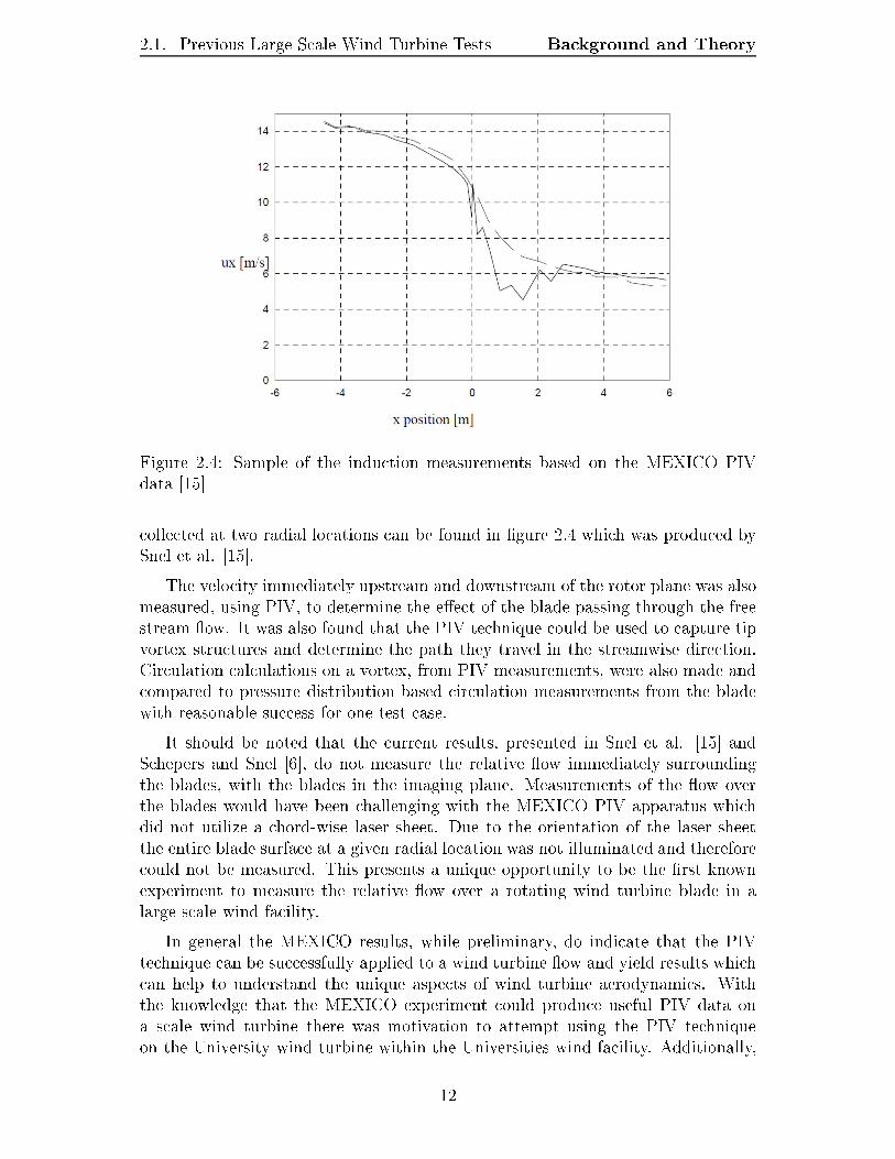
2.1. Previous Large Scale Wind Turbine Tests Background and Theory

Figure 2.4: Sample of the induction measurements based on the MEXICO PIVdata [15]collected at two radial locations can be found in gure 2.4 which was produced bySnel et al. [15].The velocity immediately upstream and downstream of the rotor plane was alsomeasured, using PIV, to determine the eect of the blade passing through the freestream ow. It was also found that the PIV technique could be used to capture tipvortex structures and determine the path they travel in the streamwise direction.Circulation calculations on a vortex, from PIV measurements, were also made andcompared to pressure distribution based circulation measurements from the bladewith reasonable success for one test case.It should be noted that the current results, presented in Snel et al. [15] andSchepers and Snel [6], do not measure the relative ow immediately surroundingthe blades, with the blades in the imaging plane. Measurements of the ow overthe blades would have been challenging with the MEXICO PIV apparatus whichdid not utilize a chord-wise laser sheet. Due to the orientation of the laser sheetthe entire blade surface at a given radial location was not illuminated and thereforecould not be measured. This presents a unique opportunity to be the rst knownexperiment to measure the relative ow over a rotating wind turbine blade in alarge scale wind facility.In general the MEXICO results, while preliminary, do indicate that the PIVtechnique can be successfully applied to a wind turbine ow and yield results whichcan help to understand the unique aspects of wind turbine aerodynamics. Withthe knowledge that the MEXICO experiment could produce useful PIV data ona scale wind turbine there was motivation to attempt using the PIV techniqueon the University wind turbine within the Universities wind facility. Additionally,12

2.2. BEM Theory and Implementation Background and Theorythe opportunity to gather velocity data at a radial location along a wind turbineblade was seen as a unique application of the PIV technique when compared to theMEXICO project.2.2 BEM Theory and Implementation2.2.1 OverviewBlade Element Momentum (BEM) theory is a tool used to estimate the aerody-namic forces on a turbine blade and, from this, estimate overall turbine loading andpower production. This technique can be employed in order to estimate the forcesthat blades could exert on a support structure prior to the blades being testedexperimentally.2.2.2 AssumptionsThe BEM theory implemented in this analysis utilized a basic model which relied ona few basic assumptions, typical for a basic BEM implementation [16], to simplifythe problem to a suitable level for initial turbine analysis. The rst assumption wasthat there is no ow radially along the blade between elements. This assumptionimplies that adjacent elements have no eect on each other. It also implies that theforce on each element is based on the lift and drag from a 2D airfoil under conditionswith identical relative velocity and angle of attack. While this assumption ignoresthe radial ow which is likely present under certain experimental ow conditions, asdiscussed in section 2.1.1.3, it was necessary in order to simplify the model; however,the error this assumption may introduce should be considered when analyzing theoutput of the model.The other main assumption, in this model, was that the incoming wind speeddid not vary based on the position of a blade in it's rotation. This eectivelyassumes that there is no wind shear or yawed ow present. Based on the tunneldesign, section 3.2, the wind shear assumption was considered valid due to the speedcontrol of the six fans and thus the wind distribution. The yawed ow condition wasdirectly controlled by orienting the rotor plane to be perpendicular to the incomingwind from the fans which results in zero yaw. Since the yaw results directly fromthe physical orientation of the wind turbine apparatus in the wind facility and thezero yaw assumption was valid.2.2.3 Procedure OverviewThe BEM procedure rst divides the blade into a user specied number of elementswhich do not aerodynamically interact with each other. The incoming wind speed13

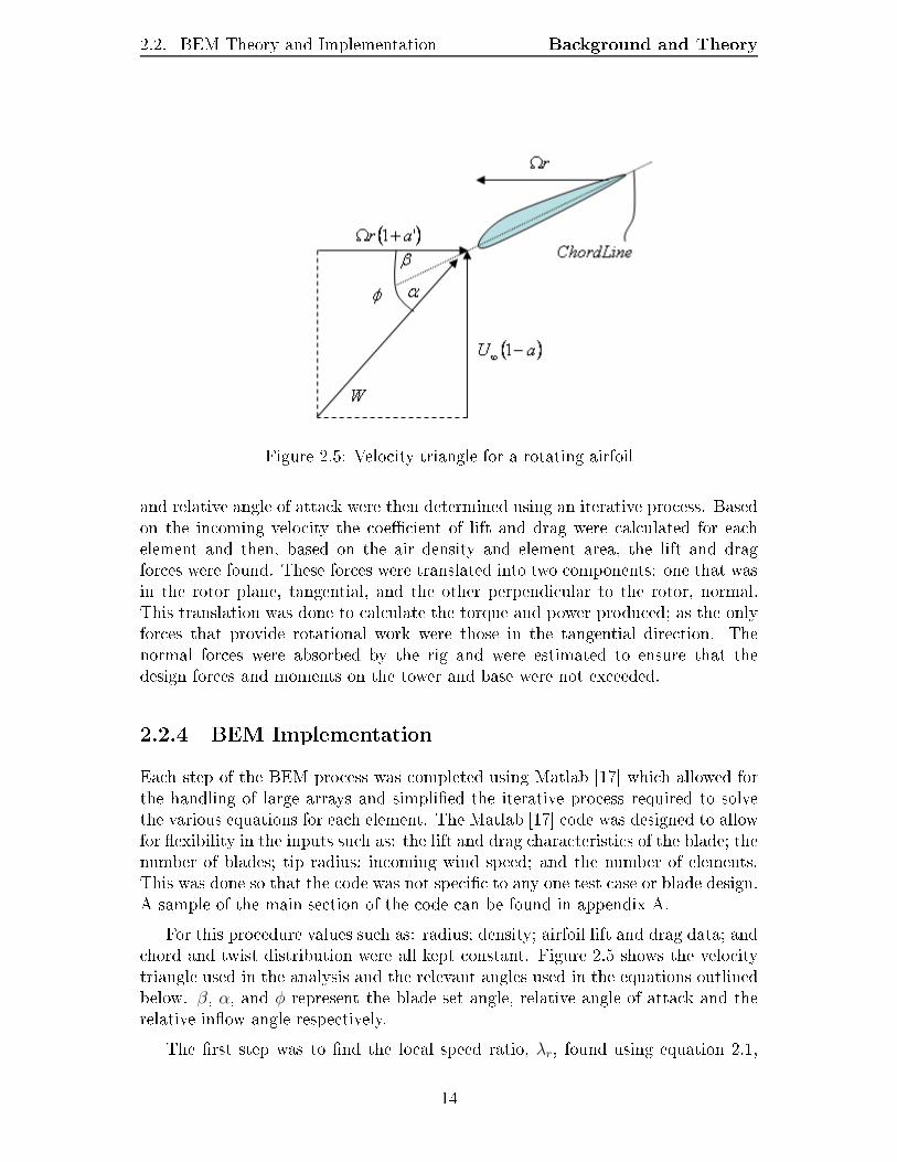
2.2. BEM Theory and Implementation Background and Theory

Figure 2.5: Velocity triangle for a rotating airfoiland relative angle of attack were then determined using an iterative process. Basedon the incoming velocity the coecient of lift and drag were calculated for eachelement and then, based on the air density and element area, the lift and dragforces were found. These forces were translated into two components: one that wasin the rotor plane, tangential, and the other perpendicular to the rotor, normal.This translation was done to calculate the torque and power produced; as the onlyforces that provide rotational work were those in the tangential direction. Thenormal forces were absorbed by the rig and were estimated to ensure that thedesign forces and moments on the tower and base were not exceeded.2.2.4 BEM ImplementationEach step of the BEM process was completed using Matlab [17] which allowed forthe handling of large arrays and simplied the iterative process required to solvethe various equations for each element. The Matlab [17] code was designed to allowfor exibility in the inputs such as: the lift and drag characteristics of the blade; thenumber of blades; tip radius; incoming wind speed; and the number of elements.This was done so that the code was not specic to any one test case or blade design.A sample of the main section of the code can be found in appendix A.For this procedure values such as: radius; density; airfoil lift and drag data; andchord and twist distribution were all kept constant. Figure 2.5 shows the velocitytriangle used in the analysis and the relevant angles used in the equations outlinedbelow. β, α, and φ represent the blade set angle, relative angle of attack and therelative inow angle respectively.The rst step was to nd the local speed ratio, λr, found using equation 2.1,14

2.2. BEM Theory and Implementation Background and Theorywith the tip speed ratio and as a function of the radius ratio of a given element.λr = λT

r

RT

(2.1)λT =

ωRT

U∞

(2.2)The next part of the code determined initial values for all parameters in eachblade element using an optimum rotor as outlined by Burton et al. [16]. Thesevalues were used as a rst guess and then iterated using the procedure outlinedbelow to nd the actual values. The optimum axial induction factor, a, was foundby maximizing the coecient of power which is derived in appendix A.1. Thisanalysis resulted in the axial induction factor initially set to 1/3 which theoreticallyresults in the maximum coecient of power of 59.3% which is called the Betz limit[16]. The induction factor, as shown in gure 2.5, eectively represents a reductionof the incoming wind speed due to the presence of a blade.Due to rotation in the wake of the rotor plane a tangential induction factor,a′, was used which eectively adds to the incoming tangential velocity due to therotation of the blades. Equation 2.3, given by Burton et al. [16], can be usedto calculate a′ as an initial value for an optimal rotor; however, for simplicity theinitial value was set to zero.

a′ =a (1 − a)

λ2r

(2.3)The inow angle, φ, was then found, using equation 2.4 which is based on thevelocity triangle geometry. Finally the relative angle of attack for each blade sectioncan be calculated, shown in equation 2.5, using the blade set angle and inow angle;with the blade set angle known by measuring the actual blade geometry. Sincethese values depend on the velocity triangle geometry the derived equations arenot dependent on an optimum rotor assumption, as such they are applicable at alllevels of this analysis.φ = tan−1

[

1 − a

λr (1 + a′)

] (2.4)α = φ − β (2.5)With the initial values set, the following equations were placed in an iterativeloop until convergence, based on the induction factor value, was reached. Theconvergence criteria was selected as a change of less than 0.01% in the axial in-duction factor based on a convergence study using the axial induction factor, withresults in section 5.2.2. Although the chord and blade set angle distributions wereset by the blade geometry the inow angle could still change based on induction15

2.2. BEM Theory and Implementation Background and Theoryfactor values and the introduction of the tip loss factor. The tip loss factor isintroduced to attempt to mimic the losses that exist at the tip of the blade. Equa-tions 2.6 through 2.10, below, were calculated for each blade element, with the codeshown in appendix A, and the relevant values were placed in an array in order to beused in force and power calculations. The equations outlined in this section weresummarized by Martinez et al. [18] which is based on work by Glauert [19] andPrandtl, given by Shen et al. [20]. The tip loss factor approaches zero at the tip,as outlined in section 5.2.3, which can cause error in the code. This error can beavoided by setting the tip loss factor at the tip to the calculated value from theprevious element.a =

1

1 + 4∗F∗sin2(φ)σ[CL cos(φ)+CD sin(φ)]

(2.6)a′ =

14∗F∗sin(φ) cos(φ)

σ[CL sin(φ)−CD cos(φ)]− 1

(2.7)F =

2

πcos−1 [exp (−1 ∗ f)] (2.8)

f =N

2

(

1 − r

RT

)

√

1 + λ2T (2.9)

σ =NC

2πr(2.10)2.2.5 Force and Power DeterminationIn order to determine the power produced by the rotor and the resulting powercoecient, CP , found using equation 2.11, various assumptions must be made. Therst is that the lift and drag, generated at the halfway point between elementstations, acts across the whole width of the element. This assumption becomesincreasingly valid as the area of the discrete element is reduced. Lastly, the innerportion of each blade was assumed to be eectively non-aerodynamic and thus doesnot detract or contribute to the overall power of the rotor.

CP =PBlade

12πρU3

∞R2

T

(2.11)The rst step to calculate the power produced was to nd the relative velocityover the blade which was then used to nd lift and drag forces, represented by the liftand drag coecients, CL and CD dened by equations 2.13 and 2.14, on each bladeelement. The forces were then translated into the tangential and normal directions,geometry shown in gure 2.6, with the tangential force used to calculate torque and16

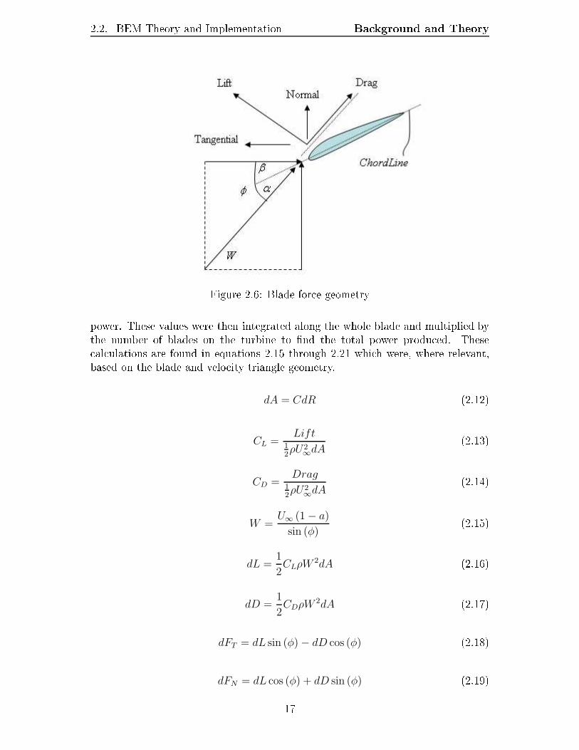
2.2. BEM Theory and Implementation Background and Theory

Figure 2.6: Blade force geometrypower. These values were then integrated along the whole blade and multiplied bythe number of blades on the turbine to nd the total power produced. Thesecalculations are found in equations 2.15 through 2.21 which were, where relevant,based on the blade and velocity triangle geometry.dA = CdR (2.12)

CL =Lift

12ρU2

∞dA

(2.13)CD =

Drag12ρU2

∞dA

(2.14)W =

U∞ (1 − a)

sin (φ)(2.15)

dL =1

2CLρW 2dA (2.16)

dD =1

2CDρW 2dA (2.17)

dFT = dL sin (φ) − dD cos (φ) (2.18)dFN = dL cos (φ) + dD sin (φ) (2.19)17

2.3. Particle Image Velocimetry Background and TheorydT = r × dFT (2.20)

dP =λT U∞

RT

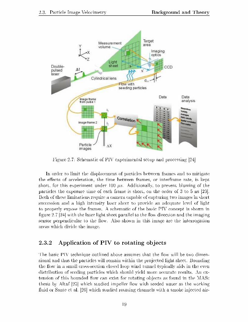
× dT (2.21)The nal step taken in the process was to complete the entire BEM procedurefor a range of tip speed ratios. This allows the ideal rotational speed for a givenwind speed to be found which maximizes CP and thus the power output of theturbine.2.3 Particle Image VelocimetryIn this section basic particle image velocimetry (PIV) theory is outlined to ac-quaint the reader with the technique utilized in this experiment with additionalinformation on the technique found in the FlowMap user's guide produced by Dan-tec Dynamics Inc. [21]. PIV is typically used in bounded ow conditions, providedby wind tunnel walls or the object being tested, and with the object being testedtypically in a stationary position; however, in this experiment PIV was used tovisualize and quantify the ow over a rotating turbine blade which was inherentlyunbounded, external and three-dimensional ow. This experiment represents aunique application of the PIV technique and as such a focus on PIV techniques formeasuring the ow on a rotating object is also presented below.2.3.1 PIV TheoryParticle image velocimetry (PIV) was developed to measure the velocity eld ofa uid ow without directly probing the ow with instrumentation. A basic PIVexperimental setup requires a high intensity two dimensional light sheet, a cameraand seeding particles in the ow. The technique captures two images, or frames,of the ow in short succession and divides each image into a user specied numberof interrogation areas. Through numerical cross-correlation, between the twocaptured frames, a representative particle displacement in each interrogation areais estimated. If the particles are assumed to travel in a linear motion, the particledisplacement divided by the time that elapsed between the captured images willdetermine the most probable velocity for each interrogation area. As the motion ofthe particles within the ow is being estimated, as opposed to the ow itself, thistechnique also assumes that the particle motion matches that of the ow. Ideallythrough careful selection of seeding particles and the method used to introduce theparticles into the ow, as outlined by Melling [22], the error introduced by this eectcan be mitigated. Finally, when the velocity vectors for all interrogation areas arecalculated an instantaneous velocity vector map is produced.18

2.3. Particle Image Velocimetry Background and Theory

Figure 2.7: Schematic of PIV experimental setup and processing [24]In order to limit the displacement of particles between frames and to mitigatethe eects of acceleration, the time between frames, or interframe rate, is keptshort, for this experiment under 100 µs. Additionally, to prevent blurring of theparticles the exposure time of each frame is short, on the order of 3 to 5 ns [23].Both of these limitations require a camera capable of capturing two images in shortsuccession and a high intensity laser sheet to provide an adequate level of lightto properly expose the frames. A schematic of the basic PIV concept is shown ingure 2.7 [24] with the laser light sheet parallel to the ow direction and the imagingsensor perpendicular to the ow. Also shown in this image are the interrogationareas which divide the image.2.3.2 Application of PIV to rotating objectsThe basic PIV technique outlined above assumes that the ow will be two dimen-sional and thus the particles will remain within the projected light sheet. Boundingthe ow in a small cross-section closed loop wind tunnel typically aids in the evendistribution of seeding particles which should yield more accurate results. An ex-tension of this bounded ow can exist for rotating objects as found in the MAScthesis by Altaf [25] which studied impeller ow with seeded water as the workinguid or Sante et al. [26] which studied rotating channels with a smoke injected air-19

2.3. Particle Image Velocimetry Background and Theoryow. Both of these studies bound the ow within rotating channels which helps tocontain the seeding particles for an even distribution. Bounded ow also providesan increased knowledge of the expected ow which can help predict ow patternsand validation of the results. Typically in rotating ows a triggering mechanism isused to allow images to be captured at specic points in the objects rotation.Unbounded external ow measurements using PIV presents unique seeding andvalidation issues. Unlike bounded ow the seeding particles are not constrained orforced to travel within the imaging area. This can produce PIV images which havelimited seeding particles with which to produce velocity data. Validation of theresults is also challenging as the ow is not conned to a set path since the owaround the blades is inherently complex as previously discussed in section 2.1.1.3.Two experiments involving rotating objects with external ow using PIV will bediscussed: the rst on a rotating airfoil within a small wind facility and the secondon a large scale rotating wind turbine blade.Work by Ferreira et al. [27] on a vertical axis wind turbine (VAWT) model ina small scale wind tunnel produced PIV results on a rotating airfoil. This workwas able to yield ow measurements at various azimuth angles and estimates of pa-rameters such as vorticity. This paper also discusses the uncertainty present whenphase averaging the ow which is a technique also used in this experiment to buildan average velocity map from numerous PIV data sets. While their results concen-trated on vorticity, it was found, as expected, that phase averaging can remove orreduce the apparent eect of small ow structures that are present in complex timedependent ows. This eect will also be present in the experimentation completedfor this project and should therefore be considered when analyzing the signicanceof any PIV results from a complex ow.As previously discussed, the MEXICO project [6, 15] was able to produce PIVresults on a rotating wind turbine which had a similar scale to the turbine usedin this experiment. Although only preliminary results have been released it wasfound that it was possible to quantify values such as induction from PIV results aswell as identifying tip vortex structures using a three dimensional PIV apparatus.While this turbine and the wind tunnel used for the MEXICO project were moreadvanced than available for this experiment it served as a basis for the types ofresearch that can be performed using the PIV technique on a wind turbine blade.With no previous research concentrating on the chordwise ow over a large scalerotating blade there was a unique opportunity to contribute a unique data set tothe research community.20

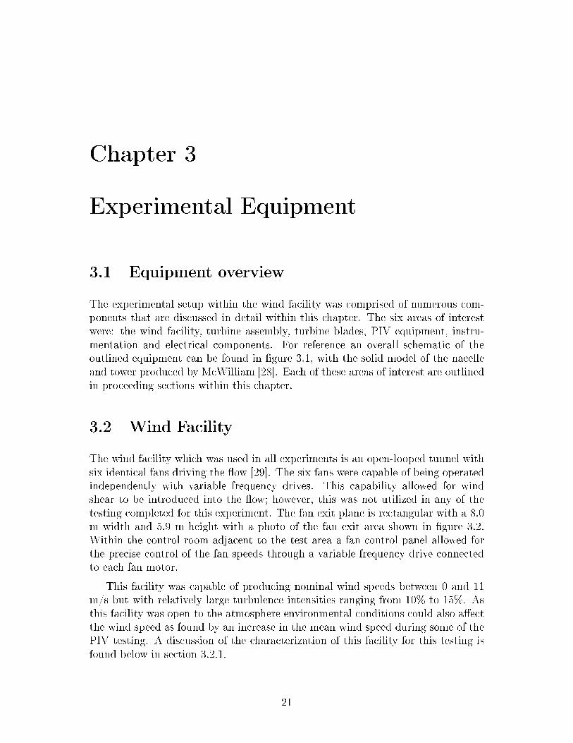
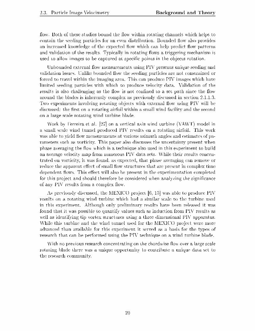
Chapter 3Experimental Equipment3.1 Equipment overviewThe experimental setup within the wind facility was comprised of numerous com-ponents that are discussed in detail within this chapter. The six areas of interestwere: the wind facility, turbine assembly, turbine blades, PIV equipment, instru-mentation and electrical components. For reference an overall schematic of theoutlined equipment can be found in gure 3.1, with the solid model of the nacelleand tower produced by McWilliam [28]. Each of these areas of interest are outlinedin proceeding sections within this chapter.3.2 Wind FacilityThe wind facility which was used in all experiments is an open-looped tunnel withsix identical fans driving the ow [29]. The six fans were capable of being operatedindependently with variable frequency drives. This capability allowed for windshear to be introduced into the ow; however, this was not utilized in any of thetesting completed for this experiment. The fan exit plane is rectangular with a 8.0m width and 5.9 m height with a photo of the fan exit area shown in gure 3.2.Within the control room adjacent to the test area a fan control panel allowed forthe precise control of the fan speeds through a variable frequency drive connectedto each fan motor.This facility was capable of producing nominal wind speeds between 0 and 11m/s but with relatively large turbulence intensities ranging from 10% to 15%. Asthis facility was open to the atmosphere environmental conditions could also aectthe wind speed as found by an increase in the mean wind speed during some of thePIV testing. A discussion of the characterization of this facility for this testing isfound below in section 3.2.1. 21

3.2. Wind Facility Experimental Equipment

Figure 3.1: Overall experimental setup: plan view

Figure 3.2: Fan exit looking from downstream22

3.2. Wind Facility Experimental Equipment

Time (s)

Vel

ocity

,UX

(m/s

)

0.0 0.1 0.2 0.3 0.4 0.5 0.6 0.7 0.8 0.9 1.06

7

8

9

10

11

12

13

14

15

16

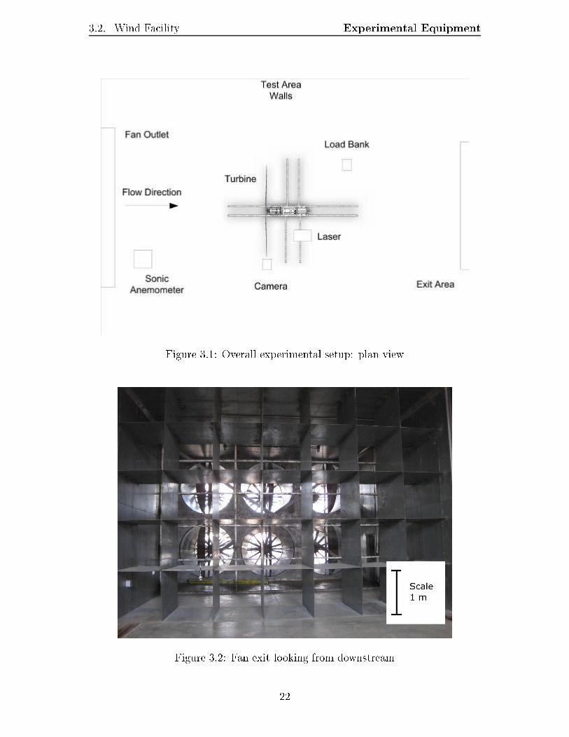
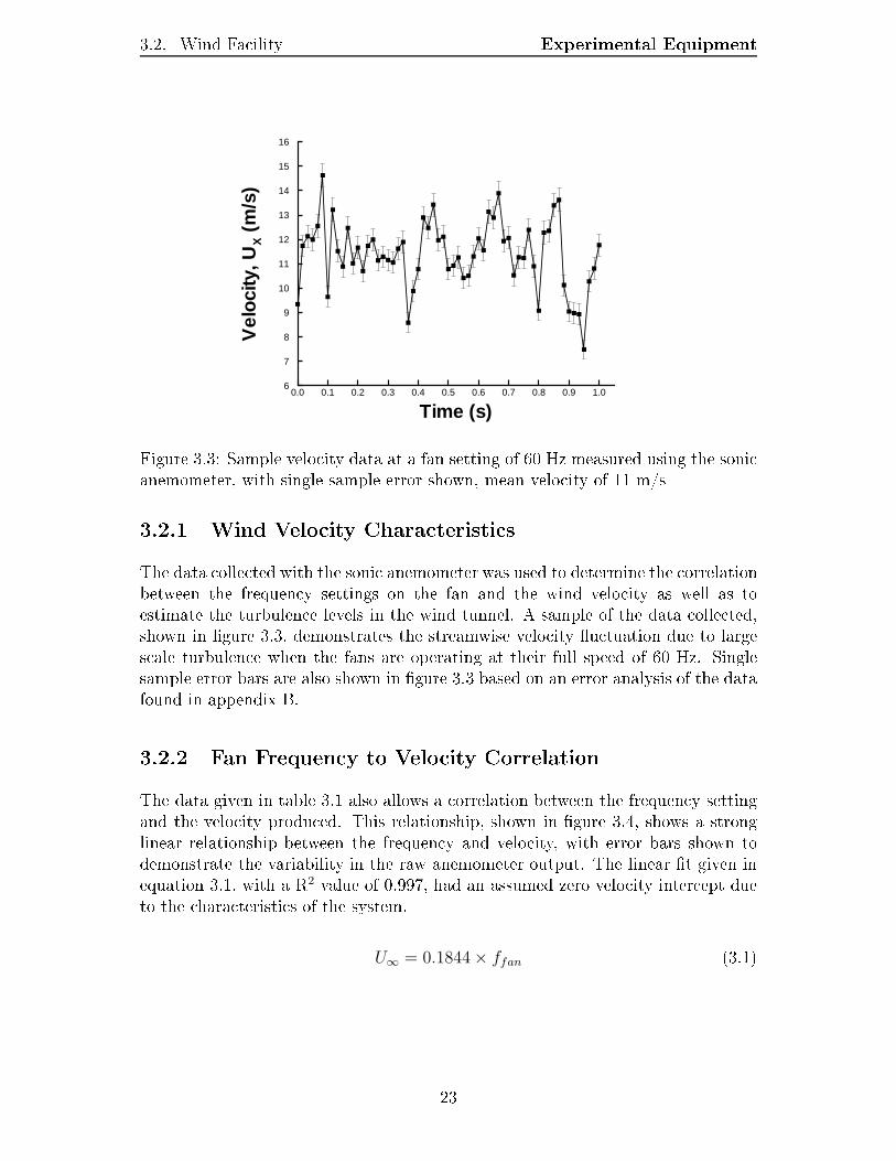
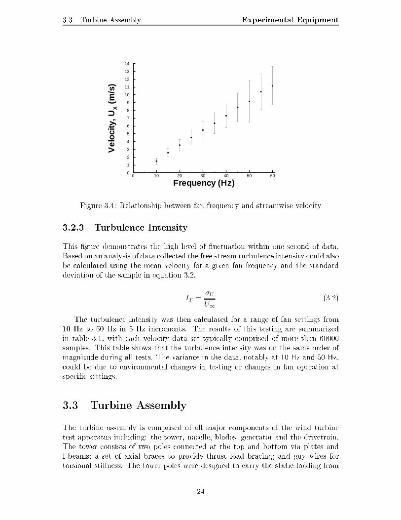
Figure 3.3: Sample velocity data at a fan setting of 60 Hz measured using the sonicanemometer, with single sample error shown, mean velocity of 11 m/s3.2.1 Wind Velocity CharacteristicsThe data collected with the sonic anemometer was used to determine the correlationbetween the frequency settings on the fan and the wind velocity as well as toestimate the turbulence levels in the wind tunnel. A sample of the data collected,shown in gure 3.3, demonstrates the streamwise velocity uctuation due to largescale turbulence when the fans are operating at their full speed of 60 Hz. Singlesample error bars are also shown in gure 3.3 based on an error analysis of the datafound in appendix B.3.2.2 Fan Frequency to Velocity CorrelationThe data given in table 3.1 also allows a correlation between the frequency settingand the velocity produced. This relationship, shown in gure 3.4, shows a stronglinear relationship between the frequency and velocity, with error bars shown todemonstrate the variability in the raw anemometer output. The linear t given inequation 3.1, with a R2 value of 0.997, had an assumed zero velocity intercept dueto the characteristics of the system.U∞ = 0.1844 × ffan (3.1)

23

3.3. Turbine Assembly Experimental Equipment

Frequency (Hz)

Vel

ocity

,UX

(m/s

)

0 10 20 30 40 50 600

1

2

3

4

5

6

7

8

9

10

11

12

13

14

Figure 3.4: Relationship between fan frequency and streamwise velocity3.2.3 Turbulence IntensityThis gure demonstrates the high level of uctuation within one second of data.Based on an analysis of data collected the free stream turbulence intensity could alsobe calculated using the mean velocity for a given fan frequency and the standarddeviation of the sample in equation 3.2.IT =

σU

U∞

(3.2)The turbulence intensity was then calculated for a range of fan settings from10 Hz to 60 Hz in 5 Hz increments. The results of this testing are summarizedin table 3.1, with each velocity data set typically comprised of more than 60000samples. This table shows that the turbulence intensity was on the same order ofmagnitude during all tests. The variance in the data, notably at 10 Hz and 50 Hz,could be due to environmental changes in testing or changes in fan operation atspecic settings.3.3 Turbine AssemblyThe turbine assembly is comprised of all major components of the wind turbinetest apparatus including: the tower, nacelle, blades, generator and the drivetrain.The tower consists of two poles connected at the top and bottom via plates andI-beams; a set of axial braces to provide thrust load bracing; and guy wires fortorsional stiness. The tower poles were designed to carry the static loading from24

3.3. Turbine Assembly Experimental EquipmentTable 3.1: Turbulence intensity over a range of fan settingsFreq(Hz)

UX

(m/s)σU

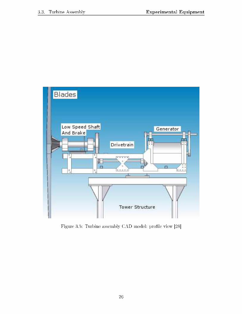
(m/s)IT10 1.49 0.19 12.73%15 2.58 0.27 10.38%20 3.55 0.36 10.18%25 4.53 0.47 10.45%30 5.48 0.58 10.60%35 6.35 0.68 10.71%40 7.31 0.78 10.67%45 8.39 0.93 11.07%50 9.15 1.37 14.93%55 10.40 1.16 11.16%60 11.14 1.25 11.27%the turbine as well as the dynamic loading from aerodynamic forces on the bladesand structure.The nacelle provides the structure and support for the blades, generator anddrivetrain. The nacelle was designed with current and future work in mind andwas bolted together, instead of welded, to allow for relatively easy dis-assemblyand modication. This nacelle and the tower support structure were designedby Michael McWilliam and this design process was extensively documented in hisMASc thesis [28]. A detailed schematic of the turbine assembly can be found ingure 3.5 along with photos of the installed assembly in gures 3.6 through 3.7. Adetailed description of the installation and decommissioning process can be foundin Appendix C.3.3.1 ModicationsSome modications were made to the original design in order to accommodate adierent blade arrangement than was originally incorporated into the nacelle andtower design. A solid model of the modied blade mounting system is shownin gure 3.8. Also safety concerns lead to the design and implementation of aemergency brake system. The blade diameter was also increased from the originaldesign and thus thrust bracing was installed to compensate for loads that couldexceed original design limits. A more detailed discussion of the brake system andthrust bracing can be found in the following sections.3.3.1.1 Brake DesignAn emergency brake was designed and connected to the low speed shaft on thenacelle. This brake was incorporated in order to have an alternative method of25

3.3. Turbine Assembly Experimental Equipment

Figure 3.5: Turbine assembly CAD model: prole view [28]

26

3.3. Turbine Assembly Experimental Equipment

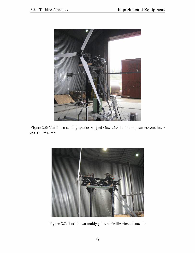
Figure 3.6: Turbine assembly photo: Angled view with load bank, camera and lasersystem in place

Figure 3.7: Turbine assembly photo: Prole view of nacelle27

3.3. Turbine Assembly Experimental Equipment

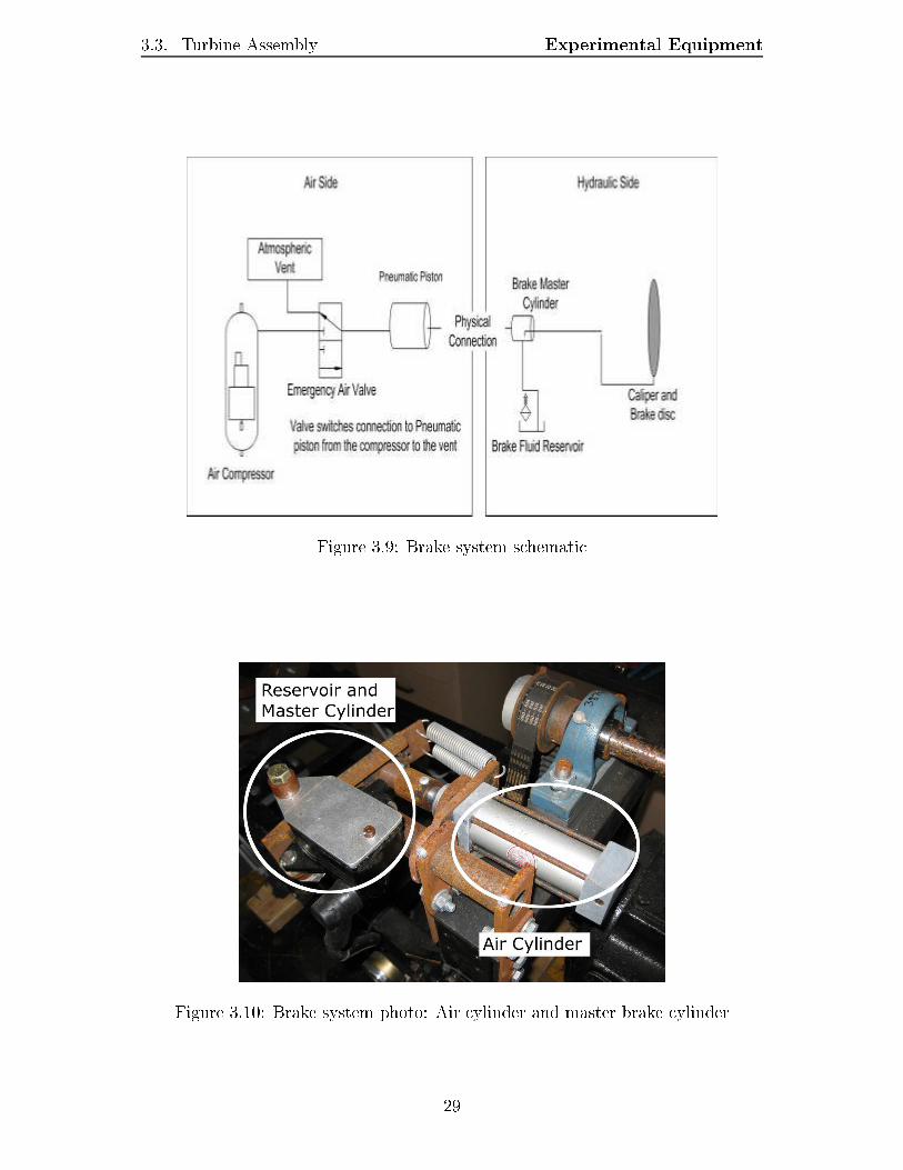
Figure 3.8: Exploded view of mounting platesstopping the rotation of the blades if the connection between the generator and theblades was broken. This could happen if any one of the three belts in the drivetrainbroke during testing or if any of the six pulleys began to slip on their shafts. Sincethe drivetrain is the connection between the blades and the generator, and thusthe primary electrical load device, if the connection was severed during a test theblades could potentially over-speed and fail.Calculations were made by a member of the wind turbine research group todetermine the torque necessary to stop the blades and a system was developedaround these required values. Due to it's compact nature and load capabilities ahydraulic brake system from a motorcycle was adapted to the test apparatus.The initial design criterion for the actuating the brake was a system which underany failure would apply the brake. It was ultimately decided that spring force wouldbe used to apply the force to the brake cylinder. Release of the brake was providedby an air cylinder which was used to extend two springs, thus removing brakingforce, from a naturally closed state. In this conguration, pressure was vented fromthe air cylinder system, through an air valve, in order to provide braking forceand if an air line were to be accidentally disconnected the brake was also applied.This conguration was almost fail safe as the only brake failure mode would bethe springs becoming disconnected from the actuator. An overall schematic of thissystem can be found in gure 3.9 with photos of the major components found ingures 3.10 to 3.11.3.3.1.2 Thrust BracingWith the increase in rotor diameter and number of blades from the original designthe estimated aerodynamic thrust loading, based on the same criteria outlined in28

3.3. Turbine Assembly Experimental Equipment

Figure 3.9: Brake system schematic

Figure 3.10: Brake system photo: Air cylinder and master brake cylinder29

3.4. Turbine Blades Experimental Equipment

Figure 3.11: Brake system photo: Calipers and disc mounted on the low speed shaftMcWilliam [28], exceeded the original design limit. The original apparatus wasdesigned for a maximum thrust of 1 kN with a safety factor of 2. The originaldesign criteria was calculated for: a wind speed of 13 m/s; a coecient of thrust,CT found in equation 3.3, of 1.2; and air density of 1.2 kg/m3. Using these samevariables the estimated thrust loading for the new blade design was found to be1.8 kN. In order to compensate for potentially higher loading members of the windturbine research group designed and constructed axial bracing which extended fromthe back of the original rig to the footing.

CT =FN

12πρV 2R2

T

(3.3)3.4 Turbine BladesThe blades manufactured for and used in this experiment were made from an ex-isting blade mould and design. A local company, Composotech [30], had a blademould in their possession which could be successfully adapted to the existing appa-ratus. Composotech could not positively identify the turbine for which the bladeswere designed; but, based on a qualitative comparison between specications andphotos, they closely resembled a blade manufactured for Southwest Windpower [31],which is a company based in Arizona. The blade outlined on the company websitematched the blade length of the manufactured blades as well as the expected energyoutput of a two bladed design, based on a BEM analysis. Southwest Windpowercould not comment on this blade specications due to the proprietary design butthrough a procedure, outlined in section 3.5, the aerodynamic properties were de-30

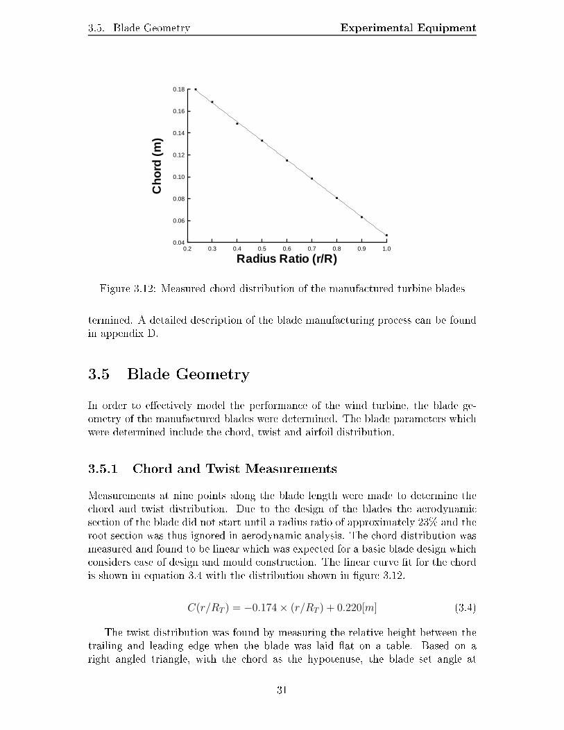
3.5. Blade Geometry Experimental Equipment

Radius Ratio (r/R)

Cho

rd(m

)

0.2 0.3 0.4 0.5 0.6 0.7 0.8 0.9 1.00.04

0.06

0.08

0.10

0.12

0.14

0.16

0.18

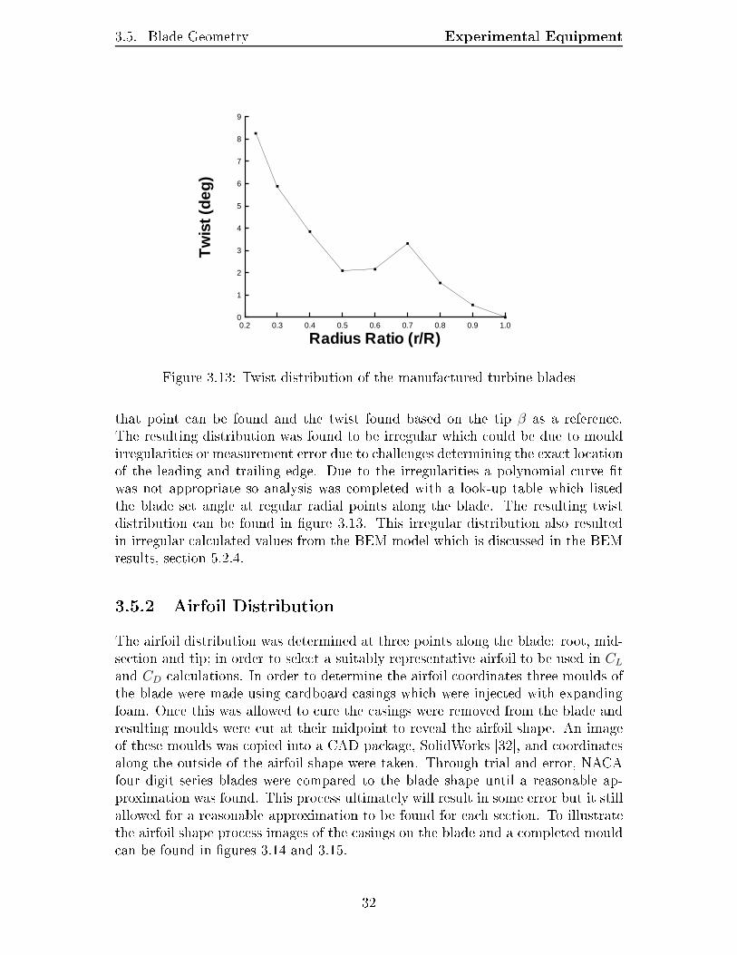
Figure 3.12: Measured chord distribution of the manufactured turbine bladestermined. A detailed description of the blade manufacturing process can be foundin appendix D.3.5 Blade GeometryIn order to eectively model the performance of the wind turbine, the blade ge-ometry of the manufactured blades were determined. The blade parameters whichwere determined include the chord, twist and airfoil distribution.3.5.1 Chord and Twist MeasurementsMeasurements at nine points along the blade length were made to determine thechord and twist distribution. Due to the design of the blades the aerodynamicsection of the blade did not start until a radius ratio of approximately 23% and theroot section was thus ignored in aerodynamic analysis. The chord distribution wasmeasured and found to be linear which was expected for a basic blade design whichconsiders ease of design and mould construction. The linear curve t for the chordis shown in equation 3.4 with the distribution shown in gure 3.12.C(r/RT ) = −0.174 × (r/RT ) + 0.220[m] (3.4)The twist distribution was found by measuring the relative height between thetrailing and leading edge when the blade was laid at on a table. Based on aright angled triangle, with the chord as the hypotenuse, the blade set angle at31

3.5. Blade Geometry Experimental Equipment

Radius Ratio (r/R)

Tw

ist(

deg

)

0.2 0.3 0.4 0.5 0.6 0.7 0.8 0.9 1.00

1

2

3

4

5

6

7

8

9

Figure 3.13: Twist distribution of the manufactured turbine bladesthat point can be found and the twist found based on the tip β as a reference.The resulting distribution was found to be irregular which could be due to mouldirregularities or measurement error due to challenges determining the exact locationof the leading and trailing edge. Due to the irregularities a polynomial curve twas not appropriate so analysis was completed with a look-up table which listedthe blade set angle at regular radial points along the blade. The resulting twistdistribution can be found in gure 3.13. This irregular distribution also resultedin irregular calculated values from the BEM model which is discussed in the BEMresults, section 5.2.4.3.5.2 Airfoil DistributionThe airfoil distribution was determined at three points along the blade: root, mid-section and tip; in order to select a suitably representative airfoil to be used in CLand CD calculations. In order to determine the airfoil coordinates three moulds ofthe blade were made using cardboard casings which were injected with expandingfoam. Once this was allowed to cure the casings were removed from the blade andresulting moulds were cut at their midpoint to reveal the airfoil shape. An imageof these moulds was copied into a CAD package, SolidWorks [32], and coordinatesalong the outside of the airfoil shape were taken. Through trial and error, NACAfour digit series blades were compared to the blade shape until a reasonable ap-proximation was found. This process ultimately will result in some error but it stillallowed for a reasonable approximation to be found for each section. To illustratethe airfoil shape process images of the casings on the blade and a completed mouldcan be found in gures 3.14 and 3.15. 32

3.5. Blade Geometry Experimental Equipment

Figure 3.14: Mould casings in place along a nished blade at the root, mid-sectionand tip

Figure 3.15: Tip mould casing removed from blade and cut at midpoint33

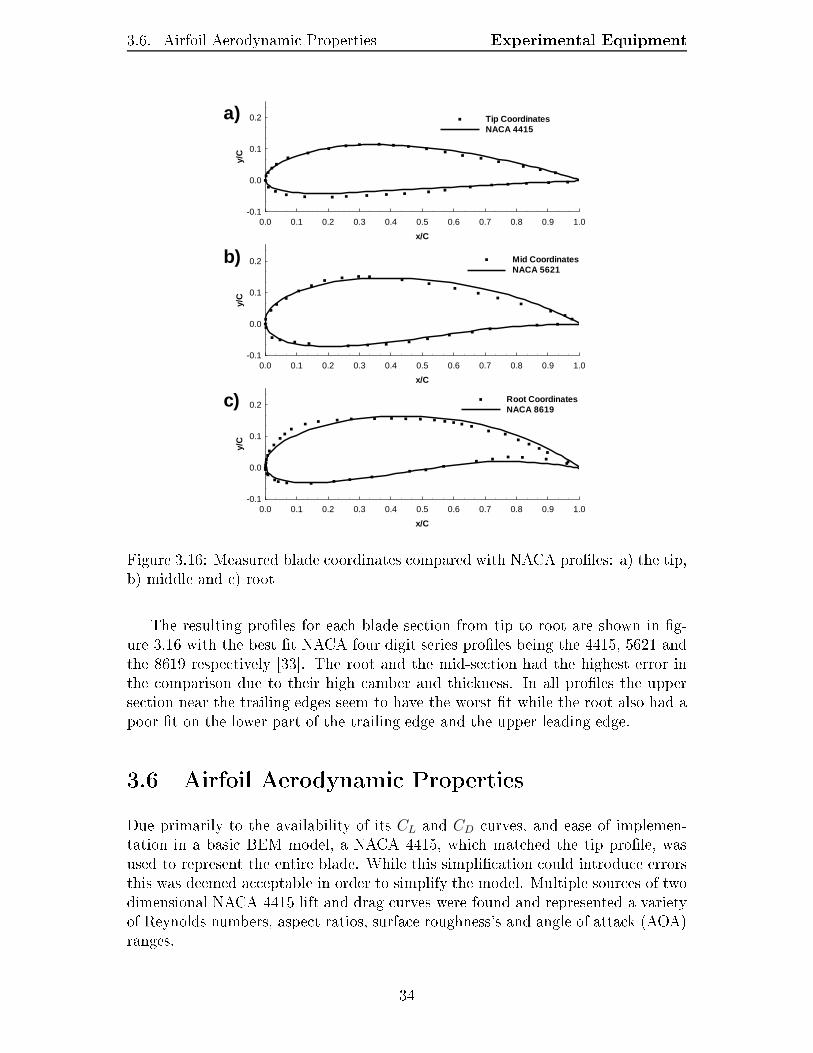
3.6. Airfoil Aerodynamic Properties Experimental Equipmentx/C

y/C

0.0 0.1 0.2 0.3 0.4 0.5 0.6 0.7 0.8 0.9 1.0-0.1

0.0

0.1

0.2 Tip CoordinatesNACA 4415

a)

x/C

y/C

0.0 0.1 0.2 0.3 0.4 0.5 0.6 0.7 0.8 0.9 1.0-0.1

0.0

0.1

0.2Root CoordinatesNACA 8619

c)x/C

y/C

0.0 0.1 0.2 0.3 0.4 0.5 0.6 0.7 0.8 0.9 1.0-0.1

0.0

0.1

0.2 Mid CoordinatesNACA 5621

b)

Figure 3.16: Measured blade coordinates compared with NACA proles: a) the tip,b) middle and c) rootThe resulting proles for each blade section from tip to root are shown in g-ure 3.16 with the best t NACA four digit series proles being the 4415, 5621 andthe 8619 respectively [33]. The root and the mid-section had the highest error inthe comparison due to their high camber and thickness. In all proles the uppersection near the trailing edges seem to have the worst t while the root also had apoor t on the lower part of the trailing edge and the upper leading edge.3.6 Airfoil Aerodynamic PropertiesDue primarily to the availability of its CL and CD curves, and ease of implemen-tation in a basic BEM model, a NACA 4415, which matched the tip prole, wasused to represent the entire blade. While this simplication could introduce errorsthis was deemed acceptable in order to simplify the model. Multiple sources of twodimensional NACA 4415 lift and drag curves were found and represented a varietyof Reynolds numbers, aspect ratios, surface roughness's and angle of attack (AOA)ranges. 34

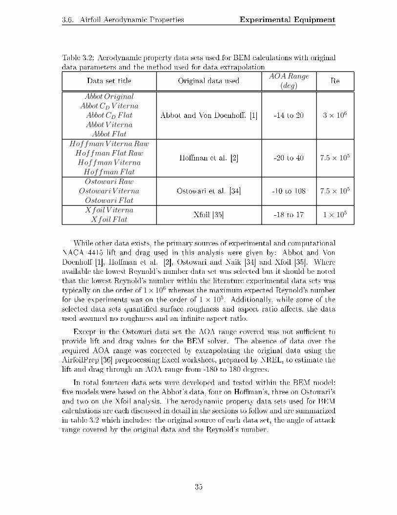
3.6. Airfoil Aerodynamic Properties Experimental EquipmentTable 3.2: Aerodynamic property data sets used for BEM calculations with originaldata parameters and the method used for data extrapolationData set title Original data used AOA Range(deg)

ReAbbot Original

Abbot CD V iternaAbbot CD F latAbbot V iterna

Abbot F lat

Abbot and Von Doenho. [1] -14 to 20 3 × 106

Hoffman V iterna RawHoffman F lat RawHoffman V iterna

Hoffman F lat

Homan et al. [2] -20 to 40 7.5 × 105

Ostowari RawOstowari V iterna

Ostowari F latOstowari et al. [34] -10 to 108 7.5 × 105

Xfoil V iternaXfoil F lat

Xfoil [35] -18 to 17 1 × 105While other data exists, the primary sources of experimental and computationalNACA 4415 lift and drag used in this analysis were given by: Abbot and VonDoenho [1], Homan et al. [2], Ostowari and Naik [34] and Xfoil [35]. Whereavailable the lowest Reynold's number data set was selected but it should be notedthat the lowest Reynold's number within the literature experimental data sets wastypically on the order of 1×106 whereas the maximum expected Reynold's numberfor the experiments was on the order of 1 × 105. Additionally, while some of theselected data sets quantied surface roughness and aspect ratio aects, the dataused assumed no roughness and an innite aspect ratio.Except in the Ostowari data set the AOA range covered was not sucient toprovide lift and drag values for the BEM solver. The absence of data over therequired AOA range was corrected by extrapolating the original data using theAirfoilPrep [36] preprocessing Excel worksheet, prepared by NREL, to estimate thelift and drag through an AOA range from -180 to 180 degrees.In total fourteen data sets were developed and tested within the BEM model:ve models were based on the Abbot's data, four on Homan's, three on Ostowari'sand two on the Xfoil analysis. The aerodynamic property data sets used for BEMcalculations are each discussed in detail in the sections to follow and are summarizedin table 3.2 which includes: the original source of each data set, the angle of attackrange covered by the original data and the Reynold's number.35

3.6. Airfoil Aerodynamic Properties Experimental Equipment3.6.1 Lift and Drag ExtrapolationThe AirfoilPrep worksheet was able to provide the tools necessary to extrapolatea given data set to encompass a full AOA range of -180 to 180 degrees. Theworksheet also contains tables to correct for three dimensional ow but this was notutilized for this basic analysis. Original AOA ranges prior to extrapolation weretypically between -10 and 20 degrees while typical AOA values required for thisBEM analysis were between -10 and 90 degrees. AirfoilPrep relies on extrapolationmethods outlined by Viterna and Janetzke [37] to predict CL and CD beyond agiven data sets maximum AOA, dened as αref .Aerodynamic property extrapolations, given in equations 3.5 and 3.6, were de-veloped by Viterna and Janetzke [37] and were used to extrapolate the aerodynamicproperties to an AOA of 90 degrees. These coecients are based on a user inputof the maximum CDmax which, by default, was calculated, using equation 3.7. TheCDmax value was based on the aspect ratio (AR) of the blade, found using equa-tion 3.8 to be 14.5.

CL =CDmax

2sin (2α) + A2

cos2 (α)

sin (α)(3.5)

CD = CDmaxsin2 (α) + B2cos (α) (3.6)where,

CDmax = 1.11 + 0.018AR (3.7)AR =

R2T

12CRT

=2RT

C(3.8)

A2 =

[

CLref −CDmax

2sin (2αref)

]

sin (αref)

cos2 (αref)(3.9)

B2 =CDref − CDmaxsin

2 (αref)

cos (αref)(3.10)Beyond 90 degrees and below the data sets minimum AOA the lift and drag co-ecients are calculated based on the original Viterna calculations but are reectedand scaled, as required, with the details of this process outlined in the AeroDyntheory and user manuals [38, 39].Alternatively, the user has the option to calculate the CD value, based on atplate theory given in equation 3.11, which relates CD to CL using the airfoil's AOA,with the CL still calculated based on the Viterna equation.

CDflat = CLtan (α) (3.11)36

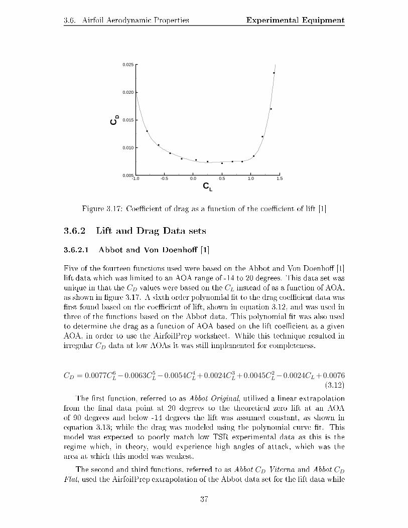
3.6. Airfoil Aerodynamic Properties Experimental Equipment

CL

CD

-1.0 -0.5 0.0 0.5 1.0 1.50.005

0.010

0.015

0.020

0.025

Figure 3.17: Coecient of drag as a function of the coecient of lift [1]3.6.2 Lift and Drag Data sets3.6.2.1 Abbot and Von Doenho [1]Five of the fourteen functions used were based on the Abbot and Von Doenho [1]lift data which was limited to an AOA range of -14 to 20 degrees. This data set wasunique in that the CD values were based on the CL instead of as a function of AOA,as shown in gure 3.17. A sixth order polynomial t to the drag coecient data wasrst found based on the coecient of lift, shown in equation 3.12, and was used inthree of the functions based on the Abbot data. This polynomial t was also usedto determine the drag as a function of AOA based on the lift coecient at a givenAOA, in order to use the AirfoilPrep worksheet. While this technique resulted inirregular CD data at low AOAs it was still implemented for completeness.CD = 0.0077C6

L−0.0063C5L−0.0054C4

L +0.0024C3L +0.0045C2

L−0.0024CL +0.0076(3.12)The rst function, referred to as Abbot Original, utilized a linear extrapolationfrom the nal data point at 20 degrees to the theoretical zero lift at an AOAof 90 degrees and below -14 degrees the lift was assumed constant, as shown inequation 3.13; while the drag was modeled using the polynomial curve t. Thismodel was expected to poorly match low TSR experimental data as this is theregime which, in theory, would experience high angles of attack, which was thearea at which this model was weakest.The second and third functions, referred to as Abbot CD Viterna and Abbot CDFlat, used the AirfoilPrep extrapolation of the Abbot data set for the lift data while37

3.6. Airfoil Aerodynamic Properties Experimental Equipmentusing the polynomial curve t for drag calculations. The nal two functions, AbbotViterna and Abbot Flat, fully utilized the AirfoilPrep worksheet to extrapolate thelift and drag data over the entire AOA range.CL(α) =

0.084615× α + 0.285 −14 < α < 14

−0.9 α ≤ −14

−0.0125 × α + 1.45 14 ≤ α ≤ 20

−0.01728 × α + 1.555 α > 20

(3.13)3.6.2.2 Homan et al. [2]Four functions were based on the Homan et al. data set [2] which extended from-20 to 40 degrees for both lift and drag. While the purpose of their study was todetermine the eects of surface roughness the data used in this study was for aclean airfoil at a Reynold's number of 0.75 × 106, which was the lowest Reynold'snumber available. All four data sets used the AirfoilPrep worksheet to extrapolatethe data; however, two of the sets used the full range of available data while theother two were extrapolated from the data covering -10 to 17 degrees. Based onthe outlined criteria, the rst two sets, extrapolated from the full available data,were referred to as Homan Viterna Raw and Homan Flat Raw with the othertwo named Homan Viterna and Homan Flat.3.6.2.3 Ostowari and Naik [34]Three functions were based on the Ostowari data set [34] which covered a rangeof -10 to 108 degrees for both lift and drag. The purpose of Ostowari's studywas to determine the aects of varying the aspect ratio over a range of Reynold'snumbers. The data set used in this BEM study were for an innite aspect ratio andat a Reynold's number of 0.75 × 106. Since the raw data from Ostowari covered asucient AOA range it was used in it's raw form, referred to as Ostowari Raw, for aBEM study. To correct for aspect ratio eects the AirfoilPrep worksheet was usedto extrapolate data from the -10 to 17 degree data range with the output referred toas Ostowari Viterna and Ostowari Flat. Completing the extrapolation also allowsa comparison of data before and after the AirfoilPrep corrections to understand it'seects.3.6.2.4 Xfoil [35]Two functions were based on the Xfoil [35] computational results which covered anangle of attack range from -18 to 17 degrees for lift and drag. A viscous model wasused with a Reynold's number of 1×105 and a mach number of 0.1. The AirfoilPrepworksheet was used to extrapolate the data with the output called Xfoil Viternaand Xfoil Flat. 38

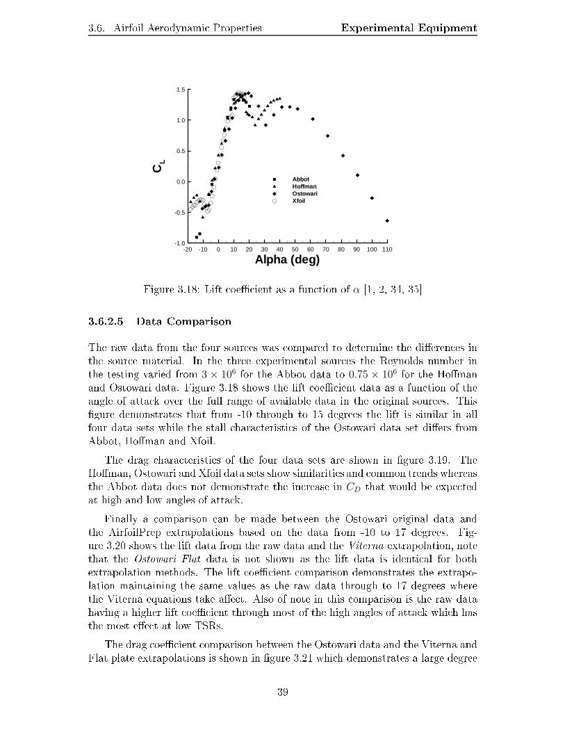
3.6. Airfoil Aerodynamic Properties Experimental Equipment

Alpha (deg)

CL

-20 -10 0 10 20 30 40 50 60 70 80 90 100 110-1.0

-0.5

0.0

0.5

1.0

1.5

AbbotHoffmanOstowariXfoil

Figure 3.18: Lift coecient as a function of α [1, 2, 34, 35]3.6.2.5 Data ComparisonThe raw data from the four sources was compared to determine the dierences inthe source material. In the three experimental sources the Reynolds number inthe testing varied from 3 × 106 for the Abbot data to 0.75 × 106 for the Homanand Ostowari data. Figure 3.18 shows the lift coecient data as a function of theangle of attack over the full range of available data in the original sources. Thisgure demonstrates that from -10 through to 15 degrees the lift is similar in allfour data sets while the stall characteristics of the Ostowari data set diers fromAbbot, Homan and Xfoil.The drag characteristics of the four data sets are shown in gure 3.19. TheHoman, Ostowari and Xfoil data sets show similarities and common trends whereasthe Abbot data does not demonstrate the increase in CD that would be expectedat high and low angles of attack.Finally a comparison can be made between the Ostowari original data andthe AirfoilPrep extrapolations based on the data from -10 to 17 degrees. Fig-ure 3.20 shows the lift data from the raw data and the Viterna extrapolation, notethat the Ostowari Flat data is not shown as the lift data is identical for bothextrapolation methods. The lift coecient comparison demonstrates the extrapo-lation maintaining the same values as the raw data through to 17 degrees wherethe Viterna equations take aect. Also of note in this comparison is the raw datahaving a higher lift coecient through most of the high angles of attack which hasthe most eect at low TSRs.The drag coecient comparison between the Ostowari data and the Viterna andFlat plate extrapolations is shown in gure 3.21 which demonstrates a large degree39

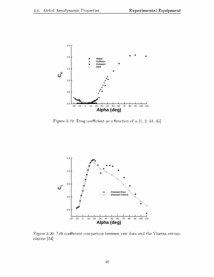
3.6. Airfoil Aerodynamic Properties Experimental Equipment

Alpha (deg)

CD

-20 -10 0 10 20 30 40 50 60 70 80 90 100 1100.0

0.5

1.0

1.5

2.0

2.5

AbbotHoffmanOstowariXfoil

Figure 3.19: Drag coecient as a function of α [1, 2, 34, 35]

Alpha (deg)

CL

-20 -10 0 10 20 30 40 50 60 70 80 90 100 110

-0.5

0.0

0.5

1.0

1.5

Ostowari RawOstowari Viterna

Figure 3.20: Lift coecient comparison between raw data and the Viterna extrap-olation [34]40

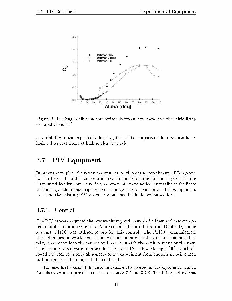
3.7. PIV Equipment Experimental Equipment

Alpha (deg)

CD

-10 0 10 20 30 40 50 60 70 80 90 100 1100.0

0.5

1.0

1.5

2.0

2.5

Ostowari RawOstowari ViternaOstowari Flat

Figure 3.21: Drag coecient comparison between raw data and the AirfoilPrepextrapolations [34]of variability in the expected value. Again in this comparison the raw data has ahigher drag coecient at high angles of attack.3.7 PIV EquipmentIn order to complete the ow measurement portion of the experiment a PIV systemwas utilized. In order to perform measurements on the rotating system in thelarge wind facility some auxiliary components were added primarily to facilitatethe timing of the image capture over a range of rotational rates. The componentsused and the existing PIV system are outlined in the following sections.3.7.1 ControlThe PIV process required the precise timing and control of a laser and camera sys-tem in order to produce results. A preassembled control box from Dantec Dynamicsystems, P1100, was utilized to provide this control. The P1100 communicated,through a local network connection, with a computer in the control room and thenrelayed commands to the camera and laser to match the settings input by the user.This requires a software interface for the user's PC, Flow Manager [40], which al-lowed the user to specify all aspects of the experiment from equipment being usedto the timing of the images to be captured.The user rst specied the laser and camera to be used in the experiment which,for this experiment, are discussed in sections 3.7.2 and 3.7.3. The ring method was41

3.7. PIV Equipment Experimental Equipmentthen selected as triggered ring; this setting will only re the system when a triggerpulse from the experimental setup was received. This ring method was utilized inthis experiment as the blades were rotating and this would limit the system to reonly when the blade was at a specic point in it's rotation.3.7.2 CameraThe camera used in the PIV setup was a Kodak Megaplus ES 1.0 camera [41]. Thepurpose of the camera, in this experiment, was to capture the seeding particlesas they traveled around the turbine blade. The PIV method required two framesto be captured with a relatively small time between the frames. This particularcamera utilizes frame straddling to achieve rapid frame rates. Instead of havingrapid shutter speeds, on the order of microseconds, this process controls the ringof a laser, the light source, to be near the end of one frame and the beginning of thenext frame. Essentially removing the control of the frame rate from the camera'sshutter and using the laser to nely adjust the inter-frame time.For this experiment the camera was held in the stationary domain while theblade rotated through the eld of view. Ultimately the camera was placed 20 cmfrom the tip and was imaging an area at a plane located 22.1 cm inboard from theblade tip which translates to a point at a radius ratio of approximately 90%. Theoverall image area was approximately 16 cm by 16 cm with the camera having aresolution of 1008 by 1018 pixels.Additionally a wavelength notch lter was placed on the camera to lter outambient light from the sun and ambient lighting in the wind facility. This lterwill only allow the wavelengths of light at 532 nm, the laser wavelength, to reachthe imaging sensor. Due to the nature of the wind facility, with large areas opento the outside atmosphere, it was crucial to remove sunlight from the images andonly image the area of interest at the blade.3.7.3 LaserThe laser in a PIV setup is the light source and must be able to output two laserpulses close together with each laser pulse lasting a short duration. As describedabove, section 3.7.2, the laser is eectively used as a shutter which is why the pulseduration must be short to avoid the particle motion being blurred. In order tohave two laser pulses close together the lasers utilized in PIV setups often have twoindependent lasing cavities. In this system a New Wave Gemini dual Nd:YAG wasoriginally used. This laser had two laser cavities each of which could produce a 130mJ laser pulse with a pulse width between 3 and 5 ns. Ultimately this laser hada critical failure and was replaced with a lower energy laser. The laser used was aNew Wave Solo II dual Nd:YAG [23] with 30 mJ energy output and a pulse widthbetween 3 and 5 ns. This laser was used as it was made by the same manufacturer42

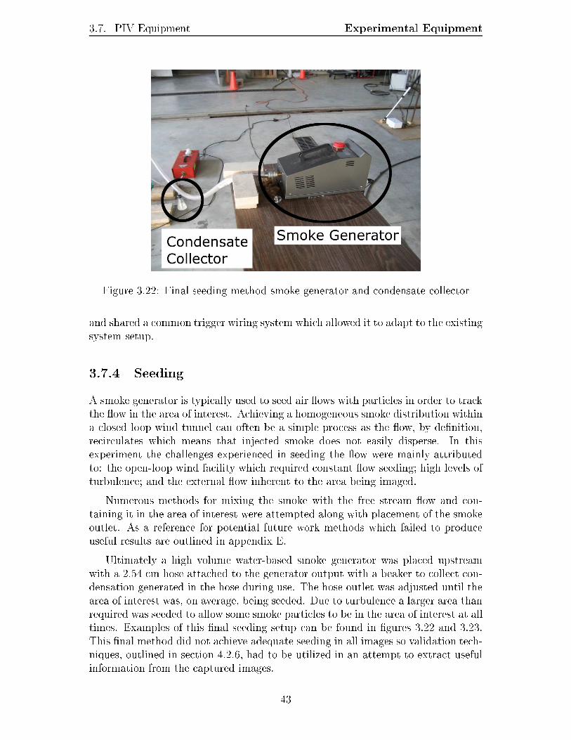
3.7. PIV Equipment Experimental Equipment

Figure 3.22: Final seeding method smoke generator and condensate collectorand shared a common trigger wiring system which allowed it to adapt to the existingsystem setup.3.7.4 SeedingA smoke generator is typically used to seed air ows with particles in order to trackthe ow in the area of interest. Achieving a homogeneous smoke distribution withina closed loop wind tunnel can often be a simple process as the ow, by denition,recirculates which means that injected smoke does not easily disperse. In thisexperiment the challenges experienced in seeding the ow were mainly attributedto: the open-loop wind facility which required constant ow seeding; high levels ofturbulence; and the external ow inherent to the area being imaged.Numerous methods for mixing the smoke with the free stream ow and con-taining it in the area of interest were attempted along with placement of the smokeoutlet. As a reference for potential future work methods which failed to produceuseful results are outlined in appendix E.Ultimately a high volume water-based smoke generator was placed upstreamwith a 2.54 cm hose attached to the generator output with a beaker to collect con-densation generated in the hose during use. The hose outlet was adjusted until thearea of interest was, on average, being seeded. Due to turbulence a larger area thanrequired was seeded to allow some smoke particles to be in the area of interest at alltimes. Examples of this nal seeding setup can be found in gures 3.22 and 3.23.This nal method did not achieve adequate seeding in all images so validation tech-niques, outlined in section 4.2.6, had to be utilized in an attempt to extract usefulinformation from the captured images. 43

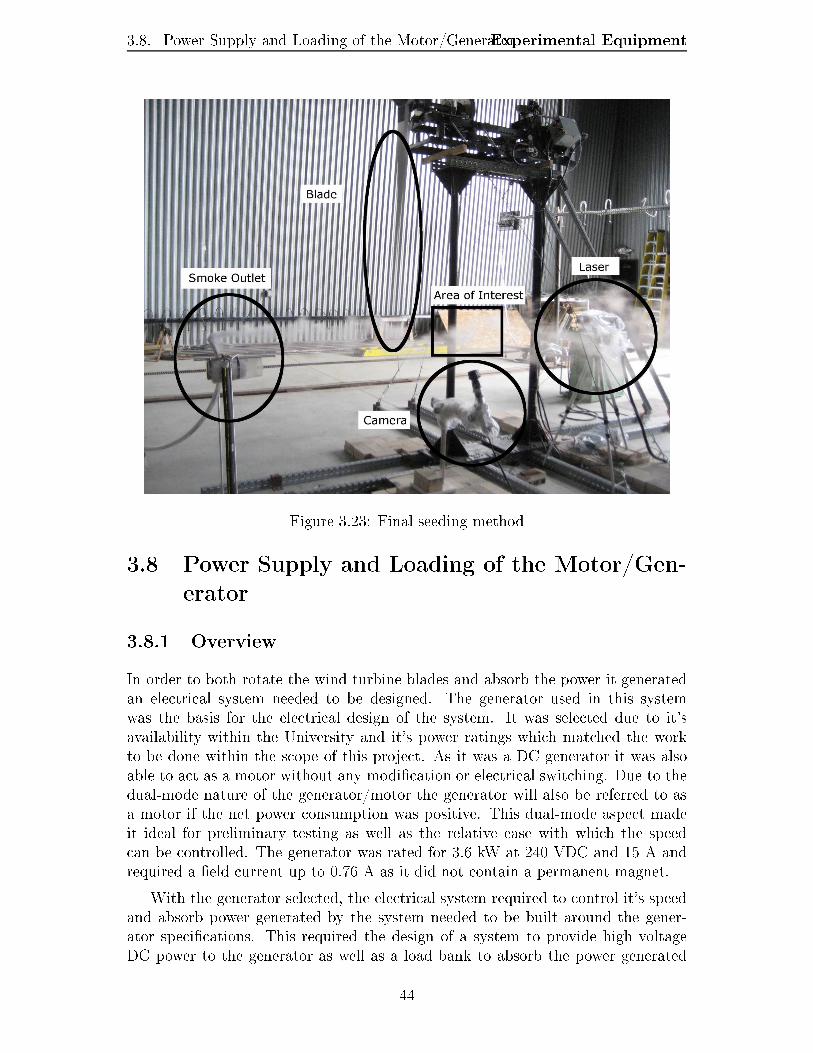
3.8. Power Supply and Loading of the Motor/GeneratorExperimental Equipment

Figure 3.23: Final seeding method3.8 Power Supply and Loading of the Motor/Gen-erator3.8.1 OverviewIn order to both rotate the wind turbine blades and absorb the power it generatedan electrical system needed to be designed. The generator used in this systemwas the basis for the electrical design of the system. It was selected due to it'savailability within the University and it's power ratings which matched the workto be done within the scope of this project. As it was a DC generator it was alsoable to act as a motor without any modication or electrical switching. Due to thedual-mode nature of the generator/motor the generator will also be referred to asa motor if the net power consumption was positive. This dual-mode aspect madeit ideal for preliminary testing as well as the relative ease with which the speedcan be controlled. The generator was rated for 3.6 kW at 240 VDC and 15 A andrequired a eld current up to 0.76 A as it did not contain a permanent magnet.With the generator selected, the electrical system required to control it's speedand absorb power generated by the system needed to be built around the gener-ator specications. This required the design of a system to provide high voltageDC power to the generator as well as a load bank to absorb the power generated44

3.8. Power Supply and Loading of the Motor/GeneratorExperimental Equipment

Figure 3.24: Electrical system wiring schematicby the blades which are outlined in sections 3.8.2 and 3.8.3. A schematic of theentire electrical system is shown in gure 3.24 with each of the components showndiscussed in further detail.3.8.2 Motor Power SupplyIn order to provide energy to the motor, which was attached to the drivetrain, thethree phase power in the wind facility needed to be converted to a DC variablepower source. The facility was equipped with three phase delta 208 VAC powerwith each leg rated for 30 A. As the power was AC it was rectied to DC using asilicon diode bridge prior to reaching the generator.For the purpose of speed control an AC variac was utilized to changed the voltagebeing fed into the rectier from 0% to 100% of the grid voltage. This allows theDC voltage to be adjusted which gave the user ne control over the motor speedas the speed of a DC motor is proportional to the armature voltage, as shown inequation 3.14.ωmotor ∝

Varm

Φ(3.14)45

3.8. Power Supply and Loading of the Motor/GeneratorExperimental EquipmentA similar system was used to power the eld with grid voltage being fed intoan independent variac and then into a silicon diode bridge before going to the eldwindings. If further speed control was required the eld voltage could be lowered,referred to as eld weakening, which results in the speed increasing. This increasein speed is due to the reduction of the magnetic ux produced by the eld whenthe eld voltage is decreased. This decrease in magnetic ux results in an increasein the motor speed, as given by the inverse relationship in equation 3.14. Caremust be taken when the eld is weakened as the armature current will increase tocompensate for the loss in ux in order to maintain constant torque, as given byequation 3.15, and could exceed the motor's rated current if not monitored.Tmotor ∝ IarmΦ (3.15)3.8.3 Generator LoadingGenerator loading was achieved by using a network of resistive elements, referred toas a load bank, to dissipate the energy generated by the turbine blades as heat. Ifthe load bank is disconnected from the generator the power produced by the bladescan not be dissipated and the blades could spin out of control and potentially fail.The load bank was comprised of various heater bars, heat coils and light bulbs,which each had a xed resistance, in order to provide a variety of loading congu-rations for future experiments. In this experiment the six heater bars available wereused exclusively as they were rated for 500 W each giving a total rated absorptionof 3000 W. A schematic of the load bank can be found below in gure 3.25 whichdemonstrates the numerous input points to connect the leads from the motor to theload bank. As previously mentioned input points one and two were used exclusivelyfor this experiment as they allowed all desired ranges of wind speed and rotationalrate to be tested.3.8.4 Wiring BoxA wiring box was mounted to the motor in order to allow easy connection to thearmature and eld leads attached to the motor. This also allowed for fusing, toprevent damaging components due to high currents, on each of the positive andnegative leads to the armature and eld windings as well as the output leads goingto the load bank. In this experiment the negative leads were not common withground and as such both positive and negative leads needed to be fused to avoida short to the grounded chassis. With reference to the overall schematic of theelectrical system, shown in gure 3.24, all of the electrical components within thewiring box are contained within the solid lines.

46

3.8. Power Supply and Loading of the Motor/GeneratorExperimental Equipment

Figure 3.25: Load bank schematic47

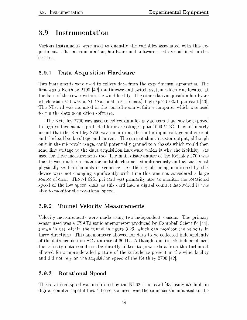
3.9. Instrumentation Experimental Equipment3.9 InstrumentationVarious instruments were used to quantify the variables associated with this ex-periment. The instrumentation, hardware and software used are outlined in thissection.3.9.1 Data Acquisition HardwareTwo instruments were used to collect data from the experimental apparatus. Therst was a Keithley 2700 [42] multimeter and switch system which was located atthe base of the tower within the wind facility. The other data acquisition hardwarewhich was used was a NI (National Instruments) high speed 6251 pci card [43].The NI card was mounted in the control room within a computer which was usedto run the data acquisition software.The Keithley 2700 was used to collect data for any sensors that may be exposedto high voltage as it is protected for over-voltage up to 1000 VDC. This ultimatelymeant that the Keithley 2700 was monitoring the motor input voltage and currentand the load bank voltage and current. The current shunt resistor output, althoughonly in the microvolt range, could potentially ground to a chassis which would thensend line voltage to the data acquisition hardware which is why the Keithley wasused for these measurements too. The main disadvantage of the Keithley 2700 wasthat it was unable to monitor multiple channels simultaneously and as such mustphysically switch channels in sequence. As the signals being monitored by thisdevice were not changing signicantly with time this was not considered a largesource of error. The NI 6251 pci card was primarily used to monitor the rotationalspeed of the low speed shaft as this card had a digital counter hardwired it wasable to monitor the rotational speed.3.9.2 Tunnel Velocity MeasurementsVelocity measurements were made using two independent sensors. The primarysensor used was a CSAT3 sonic anemometer produced by Campbell Scientic [44],shown in use within the tunnel in gure 3.26, which can monitor the velocity inthree directions. This anemometer allowed for data to be collected independentlyof the data acquisition PC at a rate of 60 Hz. Although, due to this independence,the velocity data could not be directly linked to power data from the turbine itallowed for a more detailed picture of the turbulence present in the wind facilityand did not rely on the acquisition speed of the Keithley 2700 [42].3.9.3 Rotational SpeedThe rotational speed was monitored by the NI 6251 pci card [43] using it's built-indigital counter capabilities. The sensor used was the same sensor mounted to the48

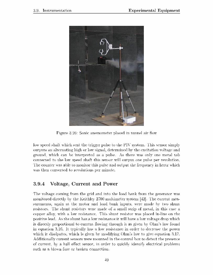
3.9. Instrumentation Experimental Equipment

Figure 3.26: Sonic anemometer placed in tunnel air owlow speed shaft which sent the trigger pulse to the PIV system. This sensor simplyoutputs an alternating high or low signal, determined by the excitation voltage andground, which can be interpreted as a pulse. As there was only one metal tabconnected to the low speed shaft this sensor will output one pulse per revolution.The counter was able to monitor this pulse and output the frequency in hertz whichwas then converted to revolutions per minute.3.9.4 Voltage, Current and PowerThe voltage coming from the grid and into the load bank from the generator wasmonitored directly by the Keithley 2700 multimeter system [42]. The current mea-surements, again at the motor and load bank inputs, were made by two shuntresistors. The shunt resistors were made of a small strip of metal, in this case acopper alloy, with a low resistance. This shunt resistor was placed in-line on thepositive lead. As the shunt has a low resistance it will have a low voltage drop whichis directly proportional to current owing through it as given by Ohm's law foundin equation 3.16. It typically has a low resistance in order to decrease the powerwhich it dissipates, which is given by modifying Ohm's law to give equation 3.17.Additionally current sensors were mounted in the control box to detect the presenceof current, by a hall eect sensor, in order to quickly identify electrical problemssuch as a blown fuse or broken connection.49

3.9. Instrumentation Experimental Equipment

Figure 3.27: Power generation schematicV = IR (3.16)

P = V I = I2R (3.17)Power was calculated using equation 3.17 from the two measured quantities atthe grid and the load bank. As seen in electrical schematic from gure 3.24 theload bank and motor are both connected, in parallel, to the grid DC input. As suchthe load bank is always drawing current from the grid as it is essentially a resistorconnected to a voltage source. In order to determine the amount of power that themotor was absorbing or producing the dierence in power between the grid inputand the load bank was determined as shown in equation 3.18. The power gener-ated can be either positive, when generating power, or negative, when motoring.Figures 3.27 and 3.28 show the generation and motoring modes schematically.PLoad = PGrid + PGEN

PGEN = PLoad − PGrid(3.18)3.9.5 Labview [45]Labview [45] was used to control the data acquisition hardware and to save thecollected data into les to be analyzed with Excel. As the Keithley 2700 was anexternal system not manufactured by NI, who also produce Labview, the commu-nication with it required more code and could not be accomplished, entirely, withbuilt in virtual instruments. The NI 6251, however, was monitored with a built-in50

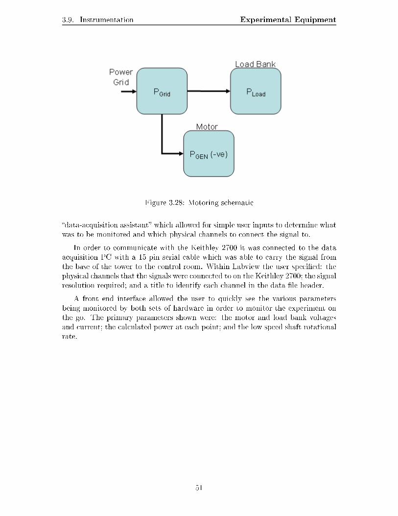
3.9. Instrumentation Experimental Equipment

Figure 3.28: Motoring schematicdata-acquisition assistant which allowed for simple user inputs to determine whatwas to be monitored and which physical channels to connect the signal to.In order to communicate with the Keithley 2700 it was connected to the dataacquisition PC with a 15 pin serial cable which was able to carry the signal fromthe base of the tower to the control room. Within Labview the user specied: thephysical channels that the signals were connected to on the Keithley 2700; the signalresolution required; and a title to identify each channel in the data le header.A front end interface allowed the user to quickly see the various parametersbeing monitored by both sets of hardware in order to monitor the experiment onthe go. The primary parameters shown were: the motor and load bank voltagesand current; the calculated power at each point; and the low speed shaft rotationalrate.

51

Chapter 4Experimental Procedure4.1 Performance MeasurementsAll performance measurements were taken using the electrical setup outlined insection 3.9.4. Both drivetrain loss and overall power production were measured asthey were key measures for future work on this experimental apparatus. Drivetrainloss was important to quantify in order to estimate the power produced at the bladesas opposed to the power measured at the generator. This relationship betweenthe measured power and the estimated power produced at the blades is found inequation 4.1. Ideally the blade power would be determined using a torque andspeed sensor at the point the blades connect to the drivetrain, instead of electricalmeasurements at the generator, but this method was not feasible with the availablematerials and test rig design.

PGEN = PAero + PDrive + PBlade (4.1)4.1.1 Drivetrain Loss EstimationThe procedure to estimate the overall power losses from rotating the blades wascompleted after all performance measurements were completed on every testing day.This procedure was completed daily in order to compensate for mechanical dier-ences due to part wear or environmental dierences due to pressure or temperaturechanges, which may aect the results.The rst step in this procedure was to ensure that the large doors at both endsof the wind facility, surrounding the test section, were closed. This was done toensure that there would be no air movement, other than self-generated, around thetest apparatus. The blades were then rotated from 40 rpm to 220 rpm in 10 rpmincrements being allowed to attain a steady state, based on power measurements,at each speed setting. As there was no wind energy input to the wind turbine,power must be drawn from the grid in order to rotate the blades. This procedure52

4.1. Performance Measurements Experimental Proceduremeasured the power loss due to aerodynamic eects and drivetrain losses, as shownin equation 5.1.PGEN(nowind) = PAero + PDrive (4.2)The same test outlined above was completed with the blades removed fromthe apparatus. This test was done in an attempt to measure the losses due onlyto the drivetrain, PDrive, as shown in equation 4.3. This particular test was onlycompleted once due to the time required to remove and reinstall the blades from theapparatus; the results were therefore presented as a percentage dierence from thelosses found with the blades attached due to the day to day environmental changes.

PGEN(noblade) = PDrive (4.3)The aerodynamic losses, due to the blade rotation, could also be quantiedby combining the results found with and without the blades attached. Equa-tion 4.4, derived from equation 4.1, demonstrates that, with no power producedat the blades, aerodynamic drag losses can also be found as the dierence of thepower measured at the motor and the drivetrain losses. The results of this testingcan be found in section 5.1.2.PAero = PGEN(nowind) − PDrive (4.4)4.1.2 Power ProductionThe power production measurements were found over a wide range of TSRs butsince the TSR was a function of both wind speed and rotational rate there arenumerous combinations of each which can result in the same TSR. Ultimatelythe number of combinations was limited due to: the wind speed limitations of thefacility; the mechanical limitations of the apparatus; and the instrumentation limitsof the speed sensor. The wind speed was limited to a mean value of approximately11 m/s, the rotational speed was limited to 220 rpm before mechanical vibrationsbecame excessive and the speed sensor could not accurately determine speeds below40 rpm. Wind speeds below 6.4 m/s, while tested, were largely ignored as the resultscontained an unacceptable level of inconsistency, likely due to the data acquisitionlimitations, as shown in the raw power curves from experiments at 3.5 m/s and6.4 m/s in gure 4.1. Low CP values at high TSRs in this gure are likely due toerroneous rotational rate data articially increasing the TSR, in the nal resultsmany of these outliers were removed using statistical criteria.The general procedure for power measurements was to set a common fan speedfor all six fans which would result in a relatively constant wind speed across therotor plane. As the fans were variable frequency drives, which were adjustable from0 to 60 Hz, the wind speed was changed in 5 Hz increments over this range. At53

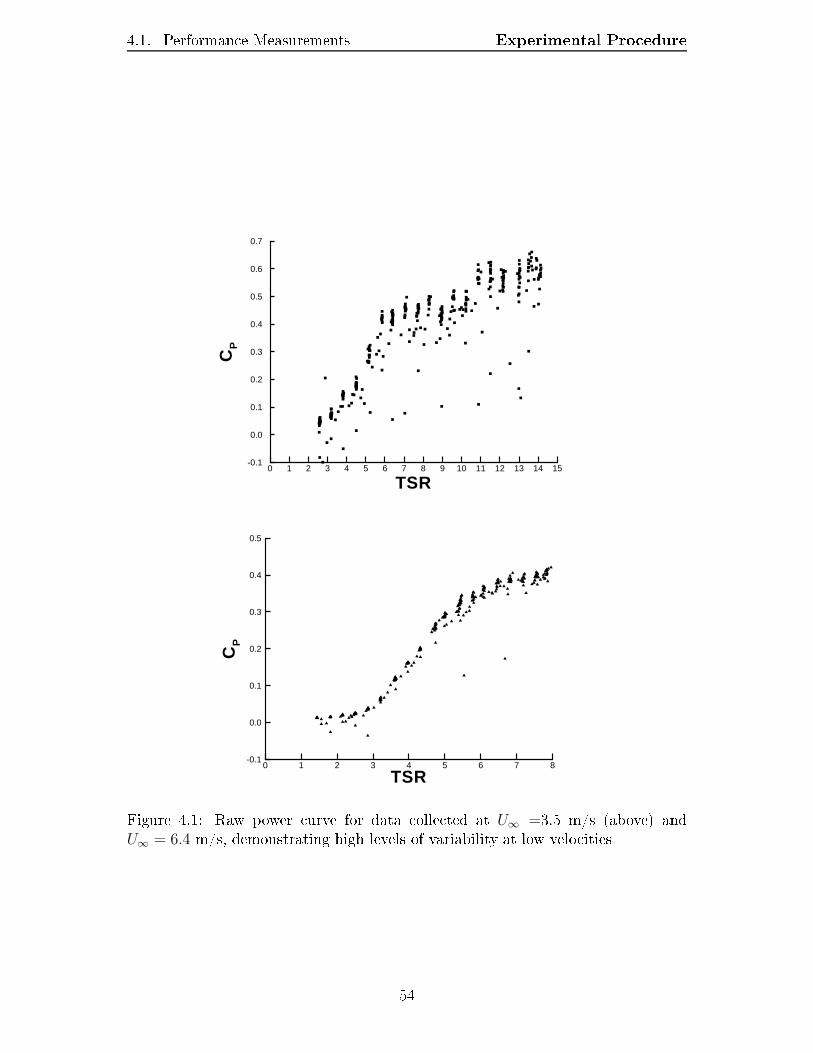
4.1. Performance Measurements Experimental Procedure

TSR

CP

0 1 2 3 4 5 6 7 8 9 10 11 12 13 14 15-0.1

0.0

0.1

0.2

0.3

0.4

0.5

0.6

0.7

TSR

CP

0 1 2 3 4 5 6 7 8-0.1

0.0

0.1

0.2

0.3

0.4

0.5

Figure 4.1: Raw power curve for data collected at U∞ =3.5 m/s (above) andU∞ = 6.4 m/s, demonstrating high levels of variability at low velocities

54

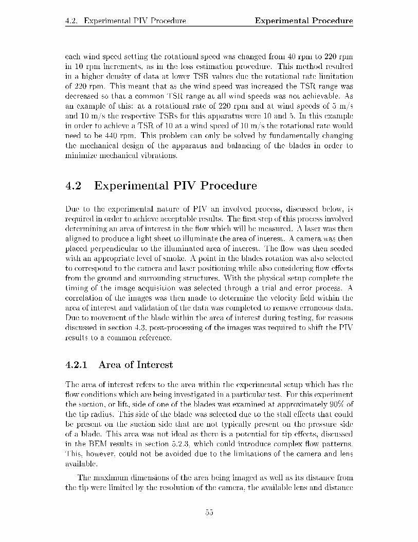
4.2. Experimental PIV Procedure Experimental Procedureeach wind speed setting the rotational speed was changed from 40 rpm to 220 rpmin 10 rpm increments, as in the loss estimation procedure. This method resultedin a higher density of data at lower TSR values due the rotational rate limitationof 220 rpm. This meant that as the wind speed was increased the TSR range wasdecreased so that a common TSR range at all wind speeds was not achievable. Asan example of this: at a rotational rate of 220 rpm and at wind speeds of 5 m/sand 10 m/s the respective TSRs for this apparatus were 10 and 5. In this examplein order to achieve a TSR of 10 at a wind speed of 10 m/s the rotational rate wouldneed to be 440 rpm. This problem can only be solved by fundamentally changingthe mechanical design of the apparatus and balancing of the blades in order tominimize mechanical vibrations.4.2 Experimental PIV ProcedureDue to the experimental nature of PIV an involved process, discussed below, isrequired in order to achieve acceptable results. The rst step of this process involveddetermining an area of interest in the ow which will be measured. A laser was thenaligned to produce a light sheet to illuminate the area of interest. A camera was thenplaced perpendicular to the illuminated area of interest. The ow was then seededwith an appropriate level of smoke. A point in the blades rotation was also selectedto correspond to the camera and laser positioning while also considering ow eectsfrom the ground and surrounding structures. With the physical setup complete thetiming of the image acquisition was selected through a trial and error process. Acorrelation of the images was then made to determine the velocity eld within thearea of interest and validation of the data was completed to remove erroneous data.Due to movement of the blade within the area of interest during testing, for reasonsdiscussed in section 4.3, post-processing of the images was required to shift the PIVresults to a common reference.4.2.1 Area of InterestThe area of interest refers to the area within the experimental setup which has theow conditions which are being investigated in a particular test. For this experimentthe suction, or lift, side of one of the blades was examined at approximately 90% ofthe tip radius. This side of the blade was selected due to the stall eects that couldbe present on the suction side that are not typically present on the pressure sideof a blade. This area was not ideal as there is a potential for tip eects, discussedin the BEM results in section 5.2.3, which could introduce complex ow patterns.This, however, could not be avoided due to the limitations of the camera and lensavailable.The maximum dimensions of the area being imaged as well as its distance fromthe tip were limited by the resolution of the camera, the available lens and distance55

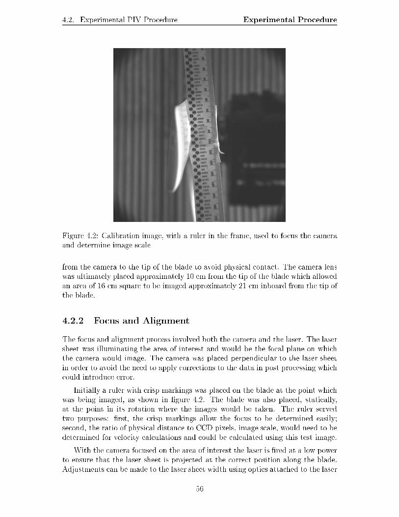
4.2. Experimental PIV Procedure Experimental Procedure

Figure 4.2: Calibration image, with a ruler in the frame, used to focus the cameraand determine image scalefrom the camera to the tip of the blade to avoid physical contact. The camera lenswas ultimately placed approximately 10 cm from the tip of the blade which allowedan area of 16 cm square to be imaged approximately 21 cm inboard from the tip ofthe blade.4.2.2 Focus and AlignmentThe focus and alignment process involved both the camera and the laser. The lasersheet was illuminating the area of interest and would be the focal plane on whichthe camera would image. The camera was placed perpendicular to the laser sheetin order to avoid the need to apply corrections to the data in post processing whichcould introduce error.Initially a ruler with crisp markings was placed on the blade at the point whichwas being imaged, as shown in gure 4.2. The blade was also placed, statically,at the point in its rotation where the images would be taken. The ruler servedtwo purposes: rst, the crisp markings allow the focus to be determined easily;second, the ratio of physical distance to CCD pixels, image scale, would need to bedetermined for velocity calculations and could be calculated using this test image.With the camera focused on the area of interest the laser is red at a low powerto ensure that the laser sheet is projected at the correct position along the blade.Adjustments can be made to the laser sheet width using optics attached to the laser56

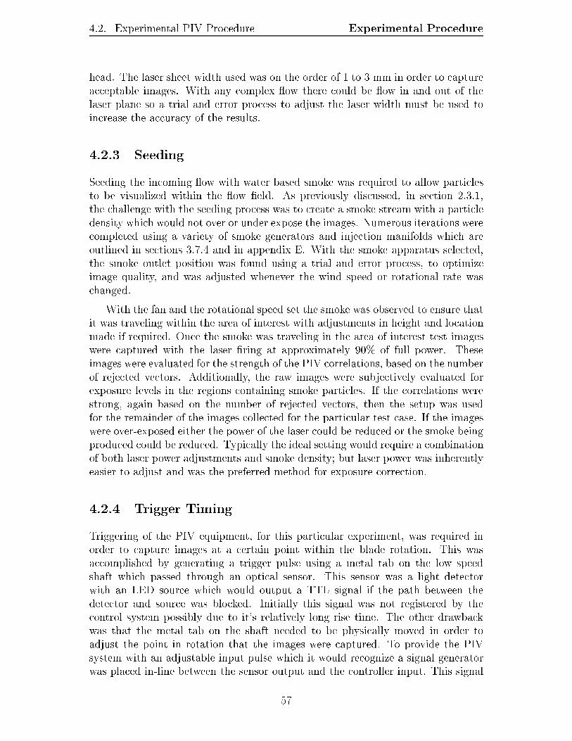
4.2. Experimental PIV Procedure Experimental Procedurehead. The laser sheet width used was on the order of 1 to 3 mm in order to captureacceptable images. With any complex ow there could be ow in and out of thelaser plane so a trial and error process to adjust the laser width must be used toincrease the accuracy of the results.4.2.3 SeedingSeeding the incoming ow with water based smoke was required to allow particlesto be visualized within the ow eld. As previously discussed, in section 2.3.1,the challenge with the seeding process was to create a smoke stream with a particledensity which would not over or under expose the images. Numerous iterations werecompleted using a variety of smoke generators and injection manifolds which areoutlined in sections 3.7.4 and in appendix E. With the smoke apparatus selected,the smoke outlet position was found using a trial and error process, to optimizeimage quality, and was adjusted whenever the wind speed or rotational rate waschanged.With the fan and the rotational speed set the smoke was observed to ensure thatit was traveling within the area of interest with adjustments in height and locationmade if required. Once the smoke was traveling in the area of interest test imageswere captured with the laser ring at approximately 90% of full power. Theseimages were evaluated for the strength of the PIV correlations, based on the numberof rejected vectors. Additionally, the raw images were subjectively evaluated forexposure levels in the regions containing smoke particles. If the correlations werestrong, again based on the number of rejected vectors, then the setup was usedfor the remainder of the images collected for the particular test case. If the imageswere over-exposed either the power of the laser could be reduced or the smoke beingproduced could be reduced. Typically the ideal setting would require a combinationof both laser power adjustments and smoke density; but laser power was inherentlyeasier to adjust and was the preferred method for exposure correction.4.2.4 Trigger TimingTriggering of the PIV equipment, for this particular experiment, was required inorder to capture images at a certain point within the blade rotation. This wasaccomplished by generating a trigger pulse using a metal tab on the low speedshaft which passed through an optical sensor. This sensor was a light detectorwith an LED source which would output a TTL signal if the path between thedetector and source was blocked. Initially this signal was not registered by thecontrol system possibly due to it's relatively long rise time. The other drawbackwas that the metal tab on the shaft needed to be physically moved in order toadjust the point in rotation that the images were captured. To provide the PIVsystem with an adjustable input pulse which it would recognize a signal generatorwas placed in-line between the sensor output and the controller input. This signal57

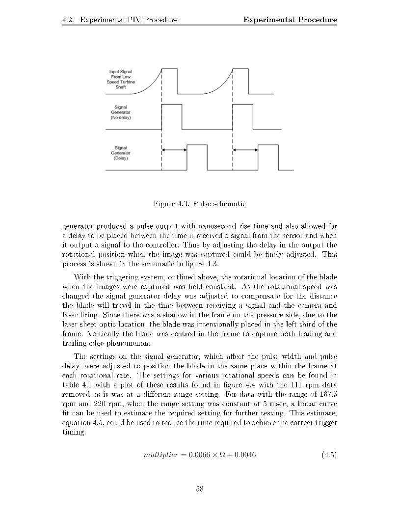
4.2. Experimental PIV Procedure Experimental Procedure

Figure 4.3: Pulse schematicgenerator produced a pulse output with nanosecond rise time and also allowed fora delay to be placed between the time it received a signal from the sensor and whenit output a signal to the controller. Thus by adjusting the delay in the output therotational position when the image was captured could be nely adjusted. Thisprocess is shown in the schematic in gure 4.3.With the triggering system, outlined above, the rotational location of the bladewhen the images were captured was held constant. As the rotational speed waschanged the signal generator delay was adjusted to compensate for the distancethe blade will travel in the time between receiving a signal and the camera andlaser ring. Since there was a shadow in the frame on the pressure side, due to thelaser sheet optic location, the blade was intentionally placed in the left third of theframe. Vertically the blade was centred in the frame to capture both leading andtrailing edge phenomenon.The settings on the signal generator, which aect the pulse width and pulsedelay, were adjusted to position the blade in the same place within the frame ateach rotational rate. The settings for various rotational speeds can be found intable 4.1 with a plot of these results found in gure 4.4 with the 111 rpm dataremoved as it was at a dierent range setting. For data with the range of 167.5rpm and 220 rpm, when the range setting was constant at 5 msec, a linear curvet can be used to estimate the required setting for further testing. This estimate,equation 4.5, could be used to reduce the time required to achieve the correct triggertiming.multiplier = 0.0066 × Ω + 0.0046 (4.5)58

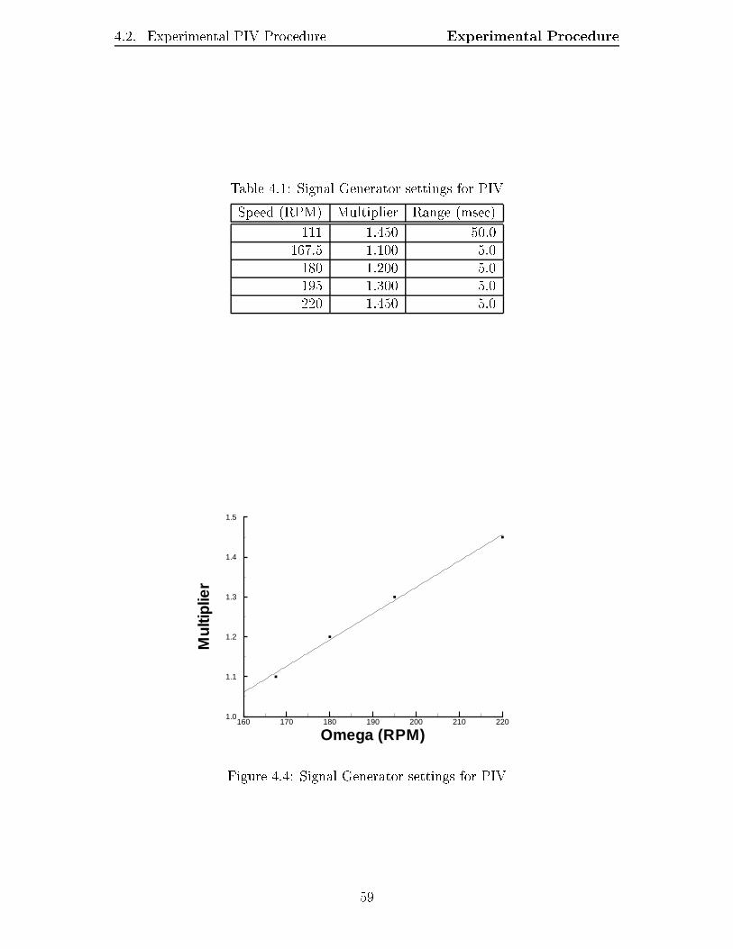
4.2. Experimental PIV Procedure Experimental ProcedureTable 4.1: Signal Generator settings for PIVSpeed (RPM) Multiplier Range (msec)111 1.450 50.0167.5 1.100 5.0180 1.200 5.0195 1.300 5.0220 1.450 5.0

Omega (RPM)

Mu

ltipl

ier

160 170 180 190 200 210 2201.0

1.1

1.2

1.3

1.4

1.5

Figure 4.4: Signal Generator settings for PIV59

4.2. Experimental PIV Procedure Experimental ProcedureTable 4.2: Theoretical and experimental interframe ratesFan Speed

(Hz)V elocity(m/s)

MaxTheo. Rate(µs)

Exp. Rate(µs)35 6.4 200 7545 8.4 152 6060 11.1 115 404.2.5 Interframe RateThe user specied the inter-frame timing which refers to the time between the twoframes, or image pairs, which are captured in each burst. The exact time betweenframes must be known in order to convert the distance a particle cloud travels to avelocity. The total number of image pairs to be captured can also be specied bythe user.The theoretical interframe rate was calculated for all wind speed and rotationalspeeds which would be used in testing. Based on theory the maximum interframerate would allow a particle to move 8 pixels, 25% of the interrogation area width,from the rst to the second frame [21]. With the pixels per metre and overallcamera resolution known from the nal focus image taken previously the maximuminterframe rate could be found using equation 4.6 from section 3.7.2. In practicethe experimental interframe rate was far below the recommended maximum valueand was found through trial and error until acceptable correlations were found foreach test case. The resulting maximum theoretical and experimental frame ratesused can be found in table 4.2.

tmax =0.00128

U∞

(4.6)Additionally, the time which will elapse between bursts can be specied. Thisvalue can either be a minimum time or based on a set number of trigger pulses.Alternatively the user can also specify the system to capture images as fast aspossible which then limits the time between bursts to the physical capabilities ofthe camera and laser. Although the system literature [41, 23] states that the cameraand laser are capable of capturing images at 15 Hz; experimentation found that theacquisition rate, on average, was between 1 Hz and 0.5 Hz. This discrepancy islikely due to the time the system requires to transfer the image data from thecamera, through the processor and into the user's computer.4.2.6 Image CorrelationThe Flow Manager software was able to take the images captured during each testand perform the cross-correlation on the image pair to produce a velocity vector60

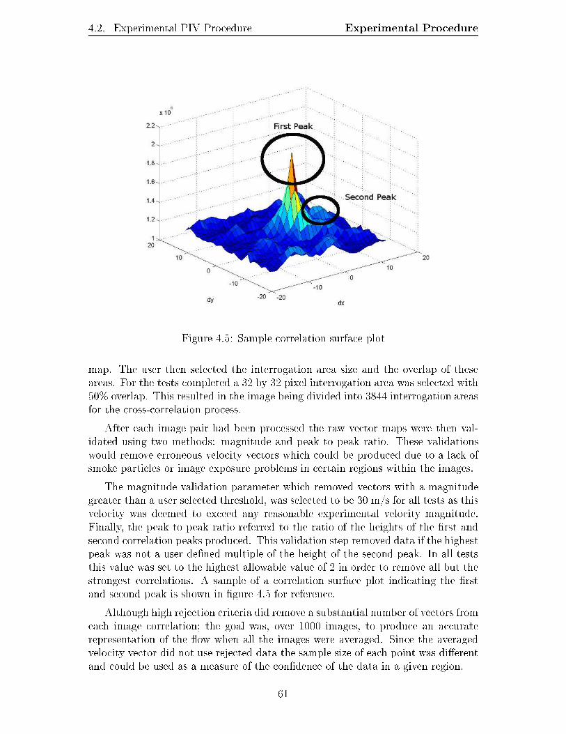
4.2. Experimental PIV Procedure Experimental Procedure

Figure 4.5: Sample correlation surface plotmap. The user then selected the interrogation area size and the overlap of theseareas. For the tests completed a 32 by 32 pixel interrogation area was selected with50% overlap. This resulted in the image being divided into 3844 interrogation areasfor the cross-correlation process.After each image pair had been processed the raw vector maps were then val-idated using two methods: magnitude and peak to peak ratio. These validationswould remove erroneous velocity vectors which could be produced due to a lack ofsmoke particles or image exposure problems in certain regions within the images.The magnitude validation parameter which removed vectors with a magnitudegreater than a user selected threshold, was selected to be 30 m/s for all tests as thisvelocity was deemed to exceed any reasonable experimental velocity magnitude.Finally, the peak to peak ratio referred to the ratio of the heights of the rst andsecond correlation peaks produced. This validation step removed data if the highestpeak was not a user dened multiple of the height of the second peak. In all teststhis value was set to the highest allowable value of 2 in order to remove all but thestrongest correlations. A sample of a correlation surface plot indicating the rstand second peak is shown in gure 4.5 for reference.Although high rejection criteria did remove a substantial number of vectors fromeach image correlation; the goal was, over 1000 images, to produce an accuraterepresentation of the ow when all the images were averaged. Since the averagedvelocity vector did not use rejected data the sample size of each point was dierentand could be used as a measure of the condence of the data in a given region.61

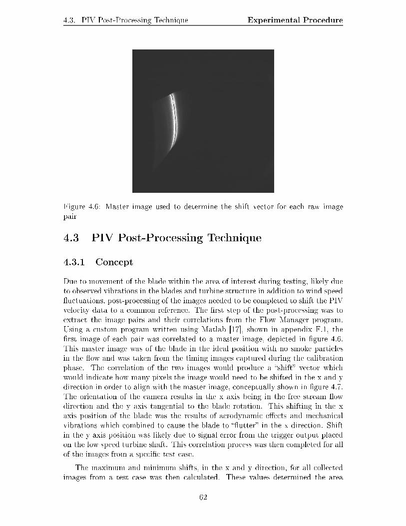
4.3. PIV Post-Processing Technique Experimental Procedure

Figure 4.6: Master image used to determine the shift vector for each raw imagepair4.3 PIV Post-Processing Technique4.3.1 ConceptDue to movement of the blade within the area of interest during testing, likely dueto observed vibrations in the blades and turbine structure in addition to wind speeductuations, post-processing of the images needed to be completed to shift the PIVvelocity data to a common reference. The rst step of the post-processing was toextract the image pairs and their correlations from the Flow Manager program.Using a custom program written using Matlab [17], shown in appendix F.1, therst image of each pair was correlated to a master image, depicted in gure 4.6.This master image was of the blade in the ideal position with no smoke particlesin the ow and was taken from the timing images captured during the calibrationphase. The correlation of the two images would produce a shift vector whichwould indicate how many pixels the image would need to be shifted in the x and ydirection in order to align with the master image, conceptually shown in gure 4.7.The orientation of the camera results in the x axis being in the free stream owdirection and the y axis tangential to the blade rotation. This shifting in the xaxis position of the blade was the results of aerodynamic eects and mechanicalvibrations which combined to cause the blade to utter in the x direction. Shiftin the y axis position was likely due to signal error from the trigger output placedon the low speed turbine shaft. This correlation process was then completed for allof the images from a specic test case.The maximum and minimum shifts, in the x and y direction, for all collectedimages from a test case was then calculated. These values determined the area62

4.3. PIV Post-Processing Technique Experimental Procedure

Figure 4.7: Shift vector conceptthat was common in all images. This concept is shown in gure 4.8 with the cross-hatched area representing the common overlap area. The cross-hatched area wouldlater be used to crop the PIV data for averaging. In order to limit the loss ofPIV data from images that were closely aligned with the master image, duringthe cropping process, two criteria were implemented to removed data. The rstcriterion was based on Chauvenet's criterion [46] which rejected data with x or yshifts that exceeded limits based on the mean, standard deviation and sample size.The second criterion removed data with a calculated shift in the x or y directionof more than 100 pixels. Both of these methods were applied in order to increasethe common area of the results. A sample of a shifted image is shown in gure 4.9,this particular image was shifted 26 pixels in the negative x direction and 50 pixelsin the negative y direction.With the shift vector for each image pair determined, the PIV data from FlowManager could be shifted to match. However, this presented a problem as the PIVcorrelation vectors are stored for each interrogation area, which were each 32 pixelssquare, and the shift results were calculated in pixels. Due to the 50% interrogationarea overlap, dened by the user, each vector represented an area 16 pixels in width.The calculated shift in pixels for each direction was therefore divided by 16 andthe results was rounded to the nearest integer; this value represented the numberof interrogation areas to move the vector prior to averaging. For example if theshift was calculated to be 36 pixels in the X direction and 57 in the Y directionthe velocity vector would get moved 2 interrogation areas to the right and 4 areasup prior to averaging. This rounding could introduce more error but with aninterrogation area every 16 pixels the maximum rounding error will be 8 pixelswhich represents approximately 1 mm. this was deemed acceptable in order toavoid the added complexity that interpolation would have added.63

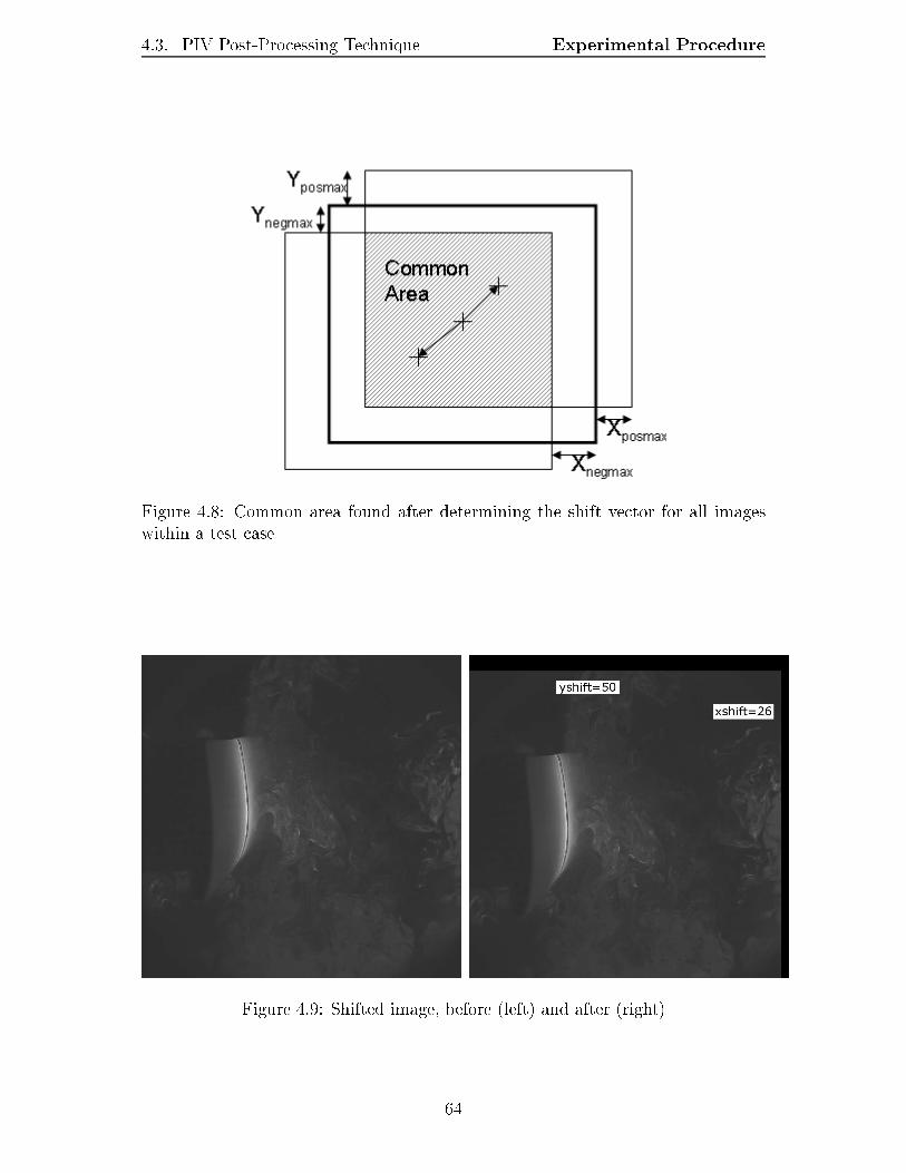
4.3. PIV Post-Processing Technique Experimental Procedure

Figure 4.8: Common area found after determining the shift vector for all imageswithin a test case

Figure 4.9: Shifted image, before (left) and after (right)64

4.3. PIV Post-Processing Technique Experimental ProcedureThe rounded shift vector was then applied to the raw PIV data which theo-retically resulted in with multiple sets of velocity data which were spatial aligned.The aligned PIV velocity vectors were then averaged to produce an overall velocitymap representative of the ow over the blade in each test case. The results of thisaveraging can be found in section 5.3.4.3.2 Image Shift Program VericationPrior to the application of the image shift program on all collected images andtheir correlations the program was rst veried against a manual determination ofthe required shift. The manual method required loading the master image and tensample images into a image editing program and manually reading coordinates of acommon point on the trailing edge of the blade within the image each image. Theimages used were from tests at the highest free stream velocity of 11.8 m/s and arotational rate of 198 rpm which were expected to represent the most variability inthe blades position due to the higher loading on the turbine.The dierence between the master image coordinates and the ten sample PIVimage coordinates can be found in table 4.3 with the values determined numericallyby the image shift program and also manually. This table also indicates the averagenumber of pixels that the images in this sample data set needed to be shifted in orderto match the master image. As previously discussed some shift values calculatedby the image shift program that exceeded the rejection criteria were removed fromconsideration as they represented a shift that was deemed excessive and likely dueto erroneous data. Rejected images in some data sets amounted to approximately30% of the original data set based on this criteria while in other data sets therejection was as low as 0.2% with the amount of rejected data independent of theow conditions. Specically in images 1 and 5, although the blade's position couldbe determined manually it could be seen that the tip of the blade was exingenough to block most of the laser light from reaching the camera and thus a strongnumerical correlation would be hard to achieve. These two images would be rejectedby the program based on the erroneous calculated shift values.Excluding the rejected values the average dierence in shift values between themanual and numerical methods was found to be approximately 8.5% in the X andY directions which in absolute terms represents 1 mm in the X direction and 0.3mm in the Y direction. While there was a discrepancy between the manual methodand the numerical approach this was deemed acceptable when also considering theshorter time required to process images and the volume of images to be processed.4.3.3 Experimental Image ProcessingThe results presented in this section attempt to show the progression from rawexperimental PIV images through to velocity vector maps of the ow over theblades. During testing approximately 1000 images at each operational state were65

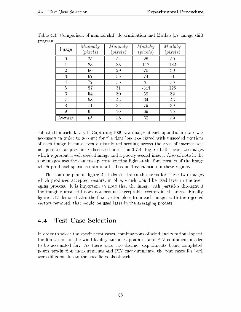
4.4. Test Case Selection Experimental ProcedureTable 4.3: Comparison of manual shift determination and Matlab [17] image shiftprogram Image ManualX(pixels)

ManualY(pixels)

MatlabX

(pixels)MatlabY

(pixels)0 25 54 26 501 83 33 117 1322 66 29 70 303 67 35 74 414 72 33 81 385 87 31 -444 1256 54 30 59 327 58 42 64 438 71 34 79 399 65 36 69 36Average 65 36 65 39collected for each data set. Capturing 1000 raw images at each operational state wasnecessary in order to account for the data loss associated with unseeded portionsof each image because evenly distributed seeding across the area of interest wasnot possible, as previously discussed in section 3.7.4. Figure 4.10 shows two imageswhich represent a well seeded image and a poorly seeded image. Also of note in theraw images was the camera aperture cutting light at the four corners of the imagewhich produced spurious data in all subsequent calculation in these regions.The contour plot in gure 4.11 demonstrates the areas for these two imageswhich produced accepted vectors, in blue, which would be used later in the aver-aging process. It is important to note that the image with particles throughoutthe imaging area still does not produce acceptable vectors in all areas. Finally,gure 4.12 demonstrates the nal vector plots from each image, with the rejectedvectors removed, that would be used later in the averaging process.4.4 Test Case SelectionIn order to select the specic test cases, combinations of wind and rotational speed,the limitations of the wind facility, turbine apparatus and PIV equipment neededto be accounted for. As there were two distinct experiments being completed,power production measurements and PIV measurements, the test cases for bothwere dierent due to the specic goals of each.66

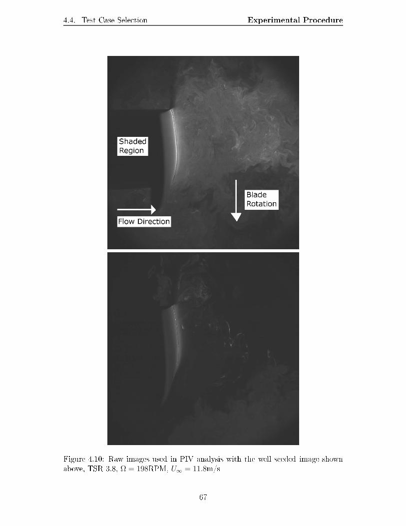
4.4. Test Case Selection Experimental Procedure

Figure 4.10: Raw images used in PIV analysis with the well seeded image shownabove, TSR 3.8, Ω = 198RPM, U∞ = 11.8m/s67

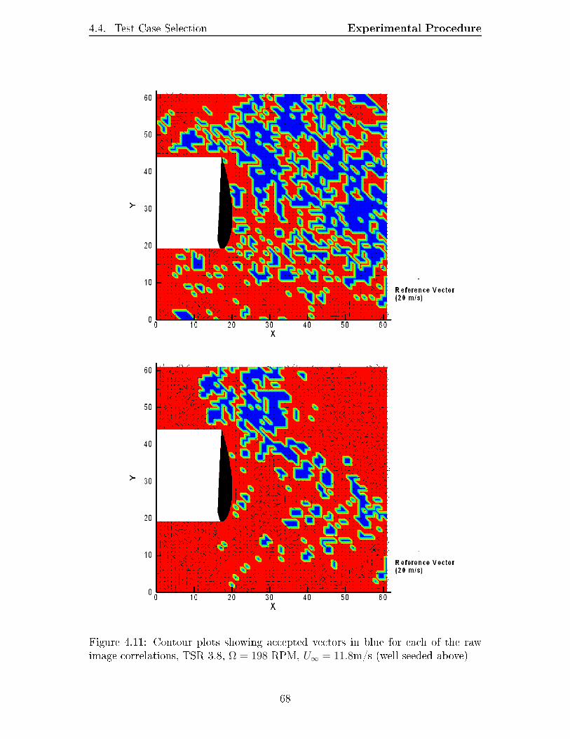
4.4. Test Case Selection Experimental Procedure

Figure 4.11: Contour plots showing accepted vectors in blue for each of the rawimage correlations, TSR 3.8, Ω = 198 RPM, U∞ = 11.8m/s (well seeded above)68

4.4. Test Case Selection Experimental Procedure

X

Y

0 10 20 30 40 50

10

20

30

40

50

Reference Vector(20 m/s)

X

Y

0 10 20 30 40 50

10

20

30

40

50

Reference Vector(20 m/s)

Figure 4.12: Vector plots from individual image pairs, TSR 3.8, Ω = 198 RPM,U∞ = 11.8m/s (well seeded above) 69

4.4. Test Case Selection Experimental ProcedureTable 4.4: Five test cases used in PIV experimentationTest number Omega (RPM) V (m/s) TSR1 195.0 11.0 42 111.0 6.4 43 167.5 6.4 64 220.0 6.4 85 220.0 7.5 64.4.1 Performance TestingAs stated previously the wind facility, in it's current conguration, was limitedto a maximum wind speed of 11 m/s. Although, based on the testing results,speeds below 6.4 m/s did not produce usable power data using the current dataacquisition system, data was still collected down to 0.5 m/s or 5 Hz on the fansettings. The turbine apparatus could not be rotated beyond 220 rpm and theacquisition system could not reliably measure the speed below 40 rpm. These valueslimited the theoretical range of TSR to between 2.5 and 13.5 for the lowest windspeed and 0.8 and 4.5 for the highest wind speed. Ultimately six wind velocitieswere chosen, nominally between 6.4 m/s and 11 m/s, which would be used in thepower production experiments to produce CP vs TSR plots.4.4.2 PIV TestingFor the PIV portion of the experiment time limitations, due to the time requiredto setup individual tests, and the mechanical limitations of the apparatus, limitingrotational speed, aected the number of tests which could be completed. Therewere two goals in the PIV portion of the testing: compare the eect of changingthe TSR value on the ow characteristics; and maintaining a constant TSR whilechanging the wind and rotational speed combination. Five test cases were selectedwhich represented four dierent rotational rates, three dierent wind speeds andthree TSRs. These ve dierent test cases were each completed on two separatedays to attempt to demonstrate repeatability of the results. Table 4.4 demonstratesthe ve test cases selected and their respective rotational speed, wind speed andresultant TSR.

70

Chapter 5Results5.1 Experimental PerformanceBased on power generation experiments conducted in the wind facility with theturbine apparatus over a range of wind speeds, 6.4 m/s to 11 m/s, and rotationalrates, 40 RPM to 220 RPM, outlined previously, the experimental performance ofthe blades could be evaluated. Drivetrain and aerodynamic power losses were rstquantied before blade power production could be evaluated.5.1.1 OutliersData pertaining to the drivetrain loss section, 5.1.2, had outlier data points, withina data set, removed using Chauvenet's criterion as suggested by Holman [46]. Sincethe measured RPM was transient each data set was taken as the nominal rotationalspeed +/- 5 rpm; for example, at a nominal rotational speed of 130 rpm, data from125 to 135 was considered part of the same data set. Chauvenet's criterion statesthat the probability of a reading, within a data set, based on a normal distribution,occurring must be greater than 1/2NS where NS is the number of readings in thedata set. This criteria was used to eliminate both outlying power and rotationalrate data.The outlier analysis was not completed for all of the blade power generationdata due to the shear volume of data present; however, the results from the 11m/s ow condition were analyzed in order to determine representative error valuesfor power generation data. The outlier analysis resulted in 4.5% of the data beingremoved from the data or 28 data points. A detailed error analysis for this dataset is outlined in appendix B.

71

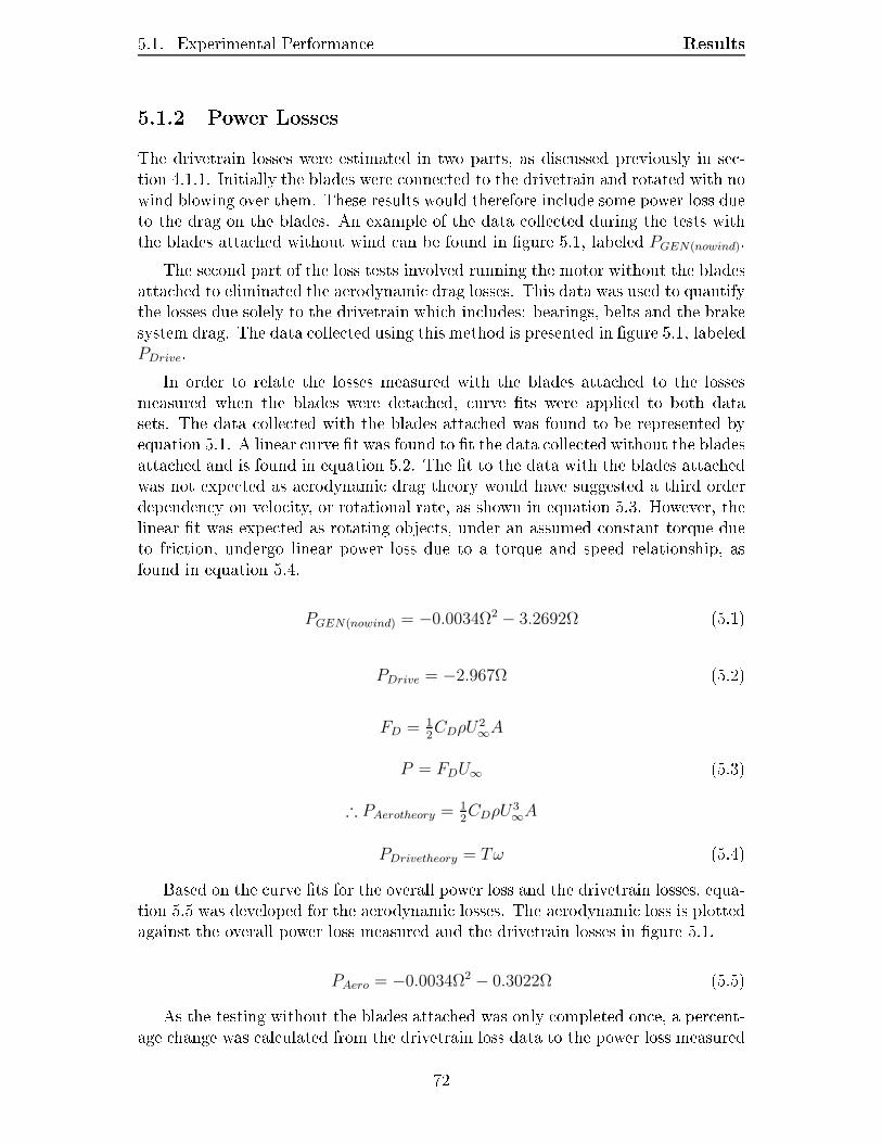
5.1. Experimental Performance Results5.1.2 Power LossesThe drivetrain losses were estimated in two parts, as discussed previously in sec-tion 4.1.1. Initially the blades were connected to the drivetrain and rotated with nowind blowing over them. These results would therefore include some power loss dueto the drag on the blades. An example of the data collected during the tests withthe blades attached without wind can be found in gure 5.1, labeled PGEN(nowind).The second part of the loss tests involved running the motor without the bladesattached to eliminated the aerodynamic drag losses. This data was used to quantifythe losses due solely to the drivetrain which includes: bearings, belts and the brakesystem drag. The data collected using this method is presented in gure 5.1, labeledPDrive.In order to relate the losses measured with the blades attached to the lossesmeasured when the blades were detached, curve ts were applied to both datasets. The data collected with the blades attached was found to be represented byequation 5.1. A linear curve t was found to t the data collected without the bladesattached and is found in equation 5.2. The t to the data with the blades attachedwas not expected as aerodynamic drag theory would have suggested a third orderdependency on velocity, or rotational rate, as shown in equation 5.3. However, thelinear t was expected as rotating objects, under an assumed constant torque dueto friction, undergo linear power loss due to a torque and speed relationship, asfound in equation 5.4.

PGEN(nowind) = −0.0034Ω2 − 3.2692Ω (5.1)PDrive = −2.967Ω (5.2)FD = 1

2CDρU2

∞A

P = FDU∞

∴ PAerotheory = 12CDρU3

∞A

(5.3)PDrivetheory = Tω (5.4)Based on the curve ts for the overall power loss and the drivetrain losses, equa-tion 5.5 was developed for the aerodynamic losses. The aerodynamic loss is plottedagainst the overall power loss measured and the drivetrain losses in gure 5.1.

PAero = −0.0034Ω2 − 0.3022Ω (5.5)As the testing without the blades attached was only completed once, a percent-age change was calculated from the drivetrain loss data to the power loss measured72

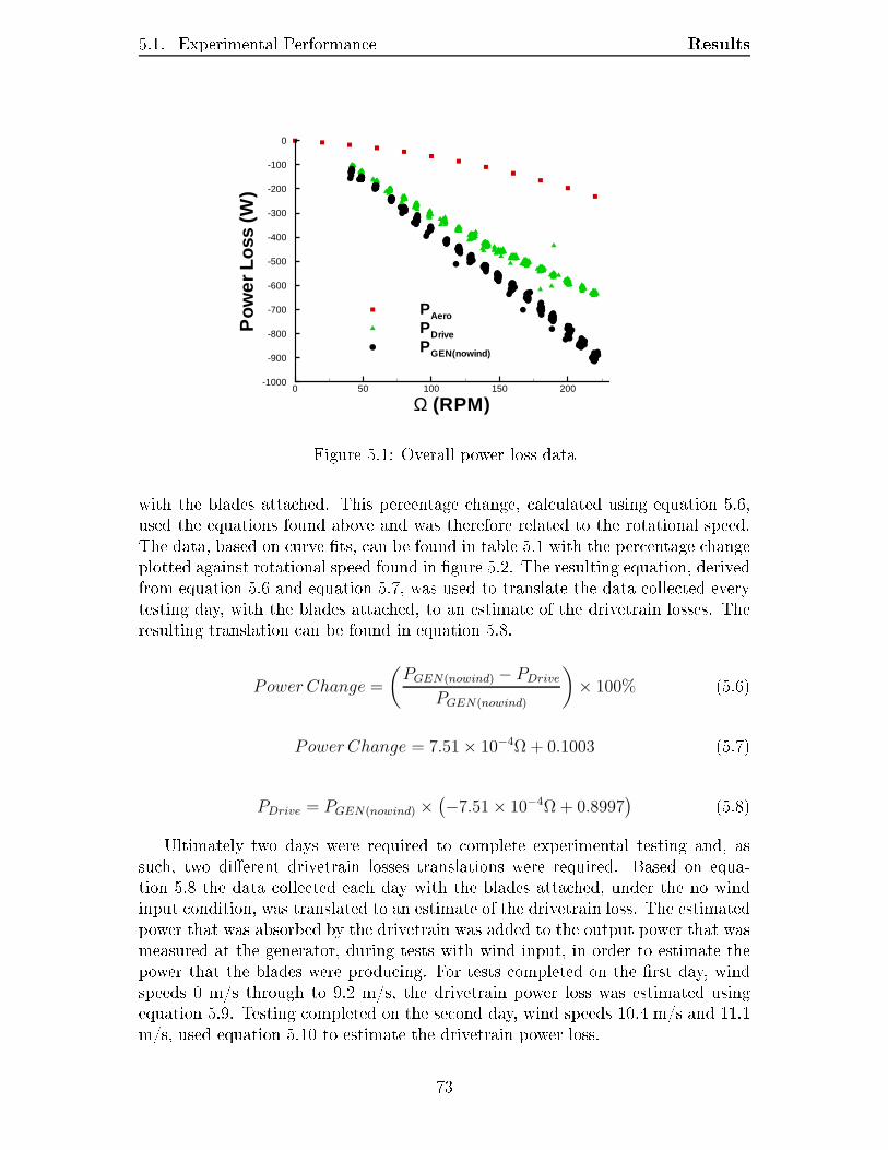
5.1. Experimental Performance Results

Ω (RPM)

Pow

erLo

ss(W

)

0 50 100 150 200-1000

-900

-800

-700

-600

-500

-400

-300

-200

-100

0

PAero

PDrive

PGEN(nowind)

Figure 5.1: Overall power loss datawith the blades attached. This percentage change, calculated using equation 5.6,used the equations found above and was therefore related to the rotational speed.The data, based on curve ts, can be found in table 5.1 with the percentage changeplotted against rotational speed found in gure 5.2. The resulting equation, derivedfrom equation 5.6 and equation 5.7, was used to translate the data collected everytesting day, with the blades attached, to an estimate of the drivetrain losses. Theresulting translation can be found in equation 5.8.Power Change =

(

PGEN(nowind) − PDrive

PGEN(nowind)

)

× 100% (5.6)Power Change = 7.51 × 10−4Ω + 0.1003 (5.7)

PDrive = PGEN(nowind) ×(

−7.51 × 10−4Ω + 0.8997) (5.8)Ultimately two days were required to complete experimental testing and, assuch, two dierent drivetrain losses translations were required. Based on equa-tion 5.8 the data collected each day with the blades attached, under the no windinput condition, was translated to an estimate of the drivetrain loss. The estimatedpower that was absorbed by the drivetrain was added to the output power that wasmeasured at the generator, during tests with wind input, in order to estimate thepower that the blades were producing. For tests completed on the rst day, windspeeds 0 m/s through to 9.2 m/s, the drivetrain power loss was estimated usingequation 5.9. Testing completed on the second day, wind speeds 10.4 m/s and 11.1m/s, used equation 5.10 to estimate the drivetrain power loss.73

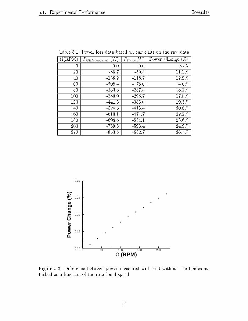
5.1. Experimental Performance ResultsTable 5.1: Power loss data based on curve ts on the raw dataΩ(RPM) PGEN(nowind) (W) PDrive(W) Power Change (%)0 0.0 0.0 N/A20 -66.7 -59.3 11.1%40 -136.2 -118.7 12.9%60 -208.4 -178.0 14.6%80 -283.3 -237.4 16.2%100 -360.9 -296.7 17.8%120 -441.3 -356.0 19.3%140 -524.3 -415.4 20.8%160 -610.1 -474.7 22.2%180 -698.6 -534.1 23.6%200 -789.8 -593.4 24.9%220 -883.8 -652.7 26.1%

Ω (RPM)

Po

wer

Ch

ange

(%)

0 50 100 150 2000.10

0.15

0.20

0.25

0.30

Figure 5.2: Dierence between power measured with and without the blades at-tached as a function of the rotational speed74

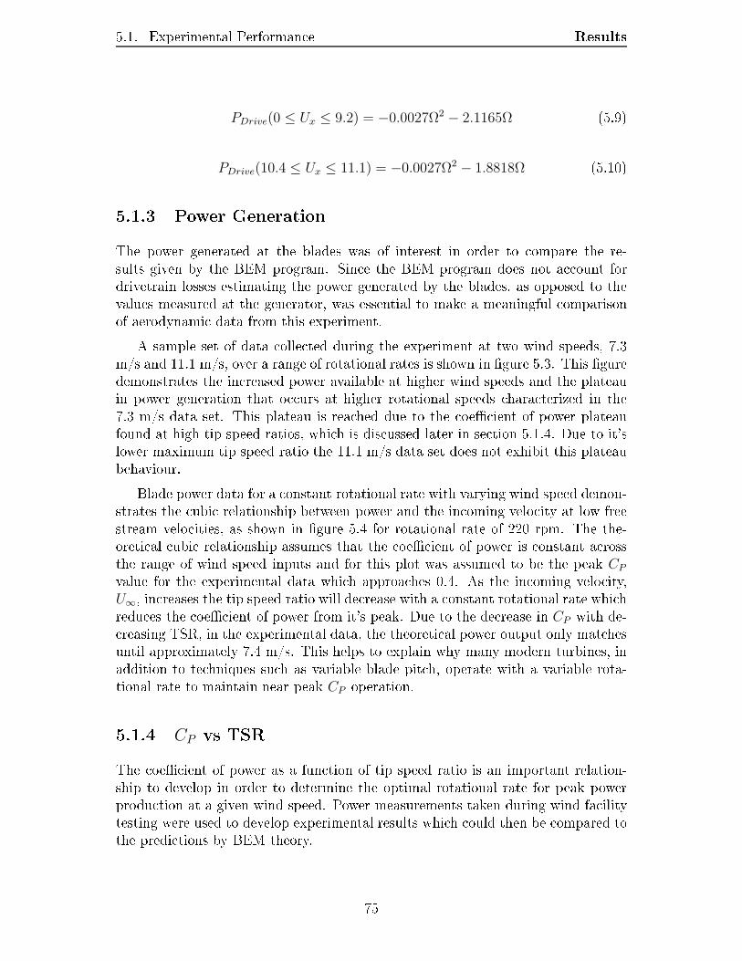
5.1. Experimental Performance ResultsPDrive(0 ≤ Ux ≤ 9.2) = −0.0027Ω2 − 2.1165Ω (5.9)

PDrive(10.4 ≤ Ux ≤ 11.1) = −0.0027Ω2 − 1.8818Ω (5.10)5.1.3 Power GenerationThe power generated at the blades was of interest in order to compare the re-sults given by the BEM program. Since the BEM program does not account fordrivetrain losses estimating the power generated by the blades, as opposed to thevalues measured at the generator, was essential to make a meaningful comparisonof aerodynamic data from this experiment.A sample set of data collected during the experiment at two wind speeds, 7.3m/s and 11.1 m/s, over a range of rotational rates is shown in gure 5.3. This guredemonstrates the increased power available at higher wind speeds and the plateauin power generation that occurs at higher rotational speeds characterized in the7.3 m/s data set. This plateau is reached due to the coecient of power plateaufound at high tip speed ratios, which is discussed later in section 5.1.4. Due to it'slower maximum tip speed ratio the 11.1 m/s data set does not exhibit this plateaubehaviour.Blade power data for a constant rotational rate with varying wind speed demon-strates the cubic relationship between power and the incoming velocity at low freestream velocities, as shown in gure 5.4 for rotational rate of 220 rpm. The the-oretical cubic relationship assumes that the coecient of power is constant acrossthe range of wind speed inputs and for this plot was assumed to be the peak CPvalue for the experimental data which approaches 0.4. As the incoming velocity,U∞, increases the tip speed ratio will decrease with a constant rotational rate whichreduces the coecient of power from it's peak. Due to the decrease in CP with de-creasing TSR, in the experimental data, the theoretical power output only matchesuntil approximately 7.4 m/s. This helps to explain why many modern turbines, inaddition to techniques such as variable blade pitch, operate with a variable rota-tional rate to maintain near peak CP operation.5.1.4 CP vs TSRThe coecient of power as a function of tip speed ratio is an important relation-ship to develop in order to determine the optimal rotational rate for peak powerproduction at a given wind speed. Power measurements taken during wind facilitytesting were used to develop experimental results which could then be compared tothe predictions by BEM theory. 75

5.1. Experimental Performance Results

Ω (RPM)

PB

lade

(W)

0 50 100 150 200 2500

500

1000

1500

2000

2500

3000

3500

11.1 m/s7.3 m/s

Figure 5.3: Power generated by the blades

Velocity, UX (m/s)

PB

lade

(W)

0 1 2 3 4 5 6 7 8 9 10 11 120

500

1000

1500

2000

2500

3000

3500

ExperimentalTheory

Figure 5.4: Power at the blades with varying wind speed, Ω= 220 rpm76

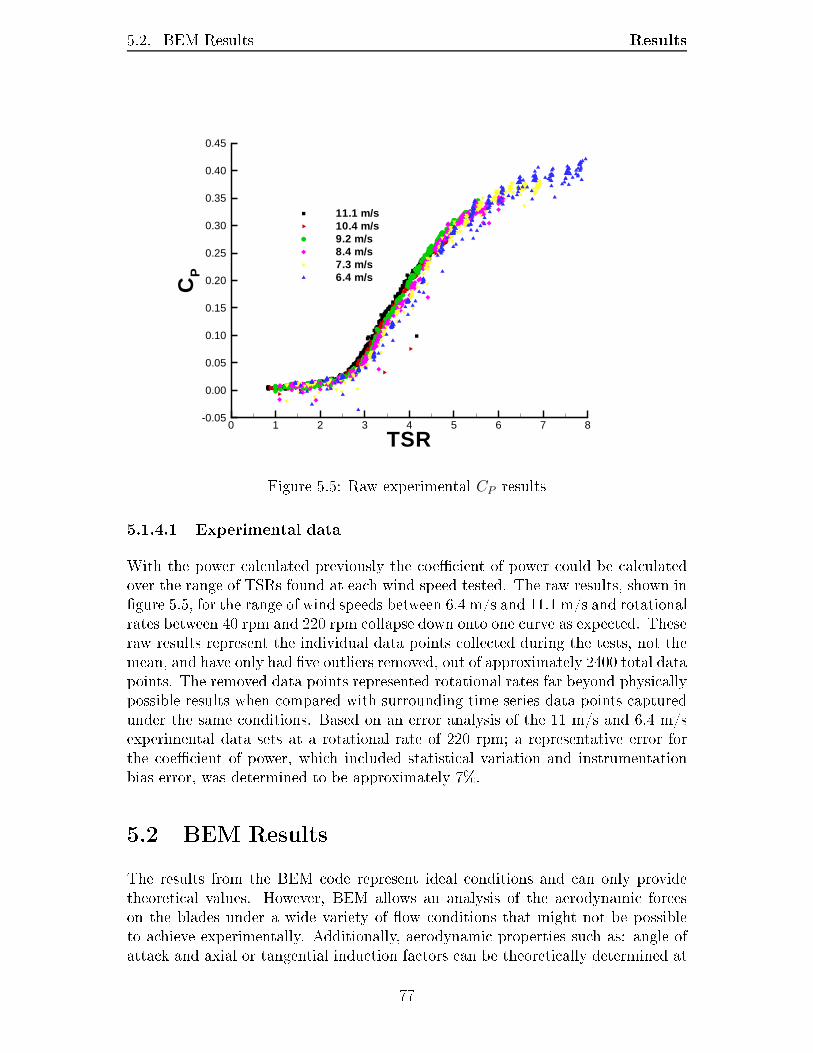
5.2. BEM Results Results

TSR

CP

0 1 2 3 4 5 6 7 8-0.05

0.00

0.05

0.10

0.15

0.20

0.25

0.30

0.35

0.40

0.45

11.1 m/s10.4 m/s9.2 m/s8.4 m/s7.3 m/s6.4 m/s

Figure 5.5: Raw experimental CP results5.1.4.1 Experimental dataWith the power calculated previously the coecient of power could be calculatedover the range of TSRs found at each wind speed tested. The raw results, shown ingure 5.5, for the range of wind speeds between 6.4 m/s and 11.1 m/s and rotationalrates between 40 rpm and 220 rpm collapse down onto one curve as expected. Theseraw results represent the individual data points collected during the tests, not themean, and have only had ve outliers removed, out of approximately 2400 total datapoints. The removed data points represented rotational rates far beyond physicallypossible results when compared with surrounding time series data points capturedunder the same conditions. Based on an error analysis of the 11 m/s and 6.4 m/sexperimental data sets at a rotational rate of 220 rpm; a representative error forthe coecient of power, which included statistical variation and instrumentationbias error, was determined to be approximately 7%.5.2 BEM ResultsThe results from the BEM code represent ideal conditions and can only providetheoretical values. However, BEM allows an analysis of the aerodynamic forceson the blades under a wide variety of ow conditions that might not be possibleto achieve experimentally. Additionally, aerodynamic properties such as: angle ofattack and axial or tangential induction factors can be theoretically determined at77

5.2. BEM Results ResultsTable 5.2: Eect of increasing the number of elementsElem Peak CPPower(W )

Peak TSR Tconverge

(s)10 0.3877 4590 9.4 450 0.3776 4470 9.2 14100 0.3757 4450 9.2 26110 0.3755 4450 9.2 29150 0.3749 4440 9.2 38200 0.3745 4440 9.2 51dierent points along the blade which are also dicult to quantify experimentally.Prior to these analyses the eect of the number of elements used in the code wasrst completed as well as a study which determined an appropriate convergencecriteria based on the axial induction factor.5.2.1 Eect of the number of elementsThe number of discrete elements, which divide the blade radially, used in the BEManalysis was determined prior to any nal results being produced. The numberof evenly spaced elements was increased until convergence, based on the CP , wasreached. Table 5.2 shows the eect of changing the number of elements on the CP ,tip speed ratio and the power produced. Although table 5.2 represents CP withfour signicant digits this is only shown to demonstrate the small changes whichwere calculated with the program as this level of accuracy could not be achieved inexperimental results. This analysis was completed for a three bladed congurationusing the Abbot Original lift and drag parameters from the manufactured bladesand a constant wind speed of 11.0 m/s as the input. At a value of 110 elementsthe CP changed by 0.05% from the previous value at 100 elements. In all furtheranalysis the blades were divided into 110 elements. The eects of increasing theelements is also shown in gure 5.6 with only the maximum CP shown, as the powergenerated changes at the same rate as the CP . The time required to run the BEMprogram was also monitored as this could have been a criterion in selecting thenumber of elements to be used.5.2.2 Axial Induction Convergence StudyA study was completed to determine the percentage change in axial induction factor,between iterations, which would be used in the BEM analysis to signify convergencefor each element. This minimum percentage change was altered from 10% to 0.1%and the eect on the CP is tabulated in table 5.3. The table shows the criterionused, the overall CP and the change in CP from the previous criterion used. It wasfound that when the criterion was changed from 10% to 0.1% only a 0.25% change78

5.2. BEM Results Results

Number of Elements

CP

0 50 100 150 2000.374

0.376

0.378

0.380

0.382

0.384

0.386

0.388

Figure 5.6: The eect of the number of elements used in the BEM analysis on theCP Table 5.3: Convergence studyConverge Criteria CP Change CP10.00% 0.3745 N/A5.00% 0.3750 0.128%1.00% 0.3754 0.099%0.50% 0.3755 0.024%0.10% 0.3755 0.003%in the CP was found. The change between a 0.5% criterion and 0.1% criterion wasfound to be 0.003% and thus 0.1% was chosen as the convergence criterion whichwould be used in the BEM analysis. The overall change of the CP between theconvergence criterion used in this study can be found in gure 5.7.5.2.3 Eects of Tip lossesFor this analysis the number of blades was set to three to correspond with thedesign which was tested in the wind facility. Also, the wind speed was again set to11.0 m/s and the number of elements set to 110 with the Abbot Original data set.The tip loss was calculated using the Prandtl tip loss factor calculation previouslyshown in section 2.2.3. This factor will increase the axial induction factor towardsthe tip of the blade which eectively reduces incoming air velocity and thus thepower that can be extracted at the tip. The tip losses can have a signicant eecton the overall power produced as the tip is the area of the blade with the mostpotential for power production. This is due to the larger amount of torque that79

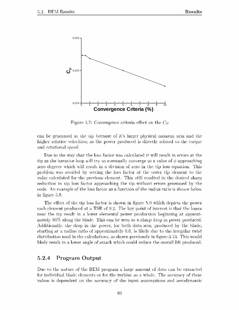
5.2. BEM Results Results

Convergence Criteria (%)

CP

0 1 2 3 4 5 6 7 8 9 100.374

0.375

0.376

Figure 5.7: Convergence criteria eect on the CPcan be generated at the tip because of it's larger physical moment arm and thehigher relative velocities; as the power produced is directly related to the torqueand rotational speed.Due to the way that the loss factor was calculated it will result in errors at thetip as the iterative loop will try to eventually converge to a value of φ approachingzero degrees which will result in a division of zero in the tip loss equation. Thisproblem was avoided by setting the loss factor at the outer tip element to thevalue calculated for the previous element. This still resulted in the desired sharpreduction in tip loss factor approaching the tip without errors generated by thecode. An example of the loss factor as a function of the radius ratio is shown belowin gure 5.8.The eect of the tip loss factor is shown in gure 5.9 which depicts the powereach element produced at a TSR of 9.2. The key point of interest is that the lossesnear the tip result in a lower elemental power production beginning at approxi-mately 80% along the blade. This can be seen as a sharp drop in power produced.Additionally, the drop in the power, for both data sets, produced by the blade,starting at a radius ratio of approximately 0.6, is likely due to the irregular twistdistribution used in the calculations, as shown previously in gure 3.13. This wouldlikely result in a lower angle of attack which could reduce the overall lift produced.5.2.4 Program OutputDue to the nature of the BEM program a large amount of data can be extractedfor individual blade elements or for the turbine as a whole. The accuracy of thesevalues is dependent on the accuracy of the input assumptions and aerodynamic80

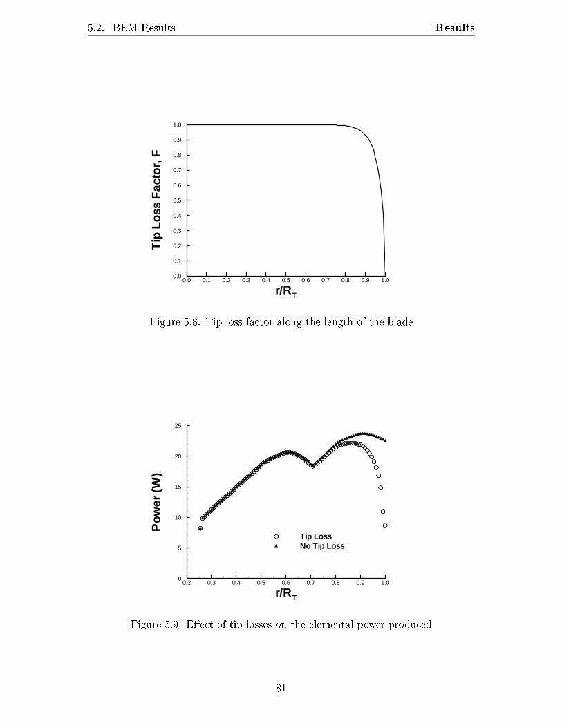
5.2. BEM Results Results

r/RT

Tip

Los

sF

acto

r,F

0.0 0.1 0.2 0.3 0.4 0.5 0.6 0.7 0.8 0.9 1.00.0

0.1

0.2

0.3

0.4

0.5

0.6

0.7

0.8

0.9

1.0

Figure 5.8: Tip loss factor along the length of the blade

r/RT

Pow

er(W

)

0.2 0.3 0.4 0.5 0.6 0.7 0.8 0.9 1.00

5

10

15

20

25

Tip LossNo Tip Loss

Figure 5.9: Eect of tip losses on the elemental power produced81

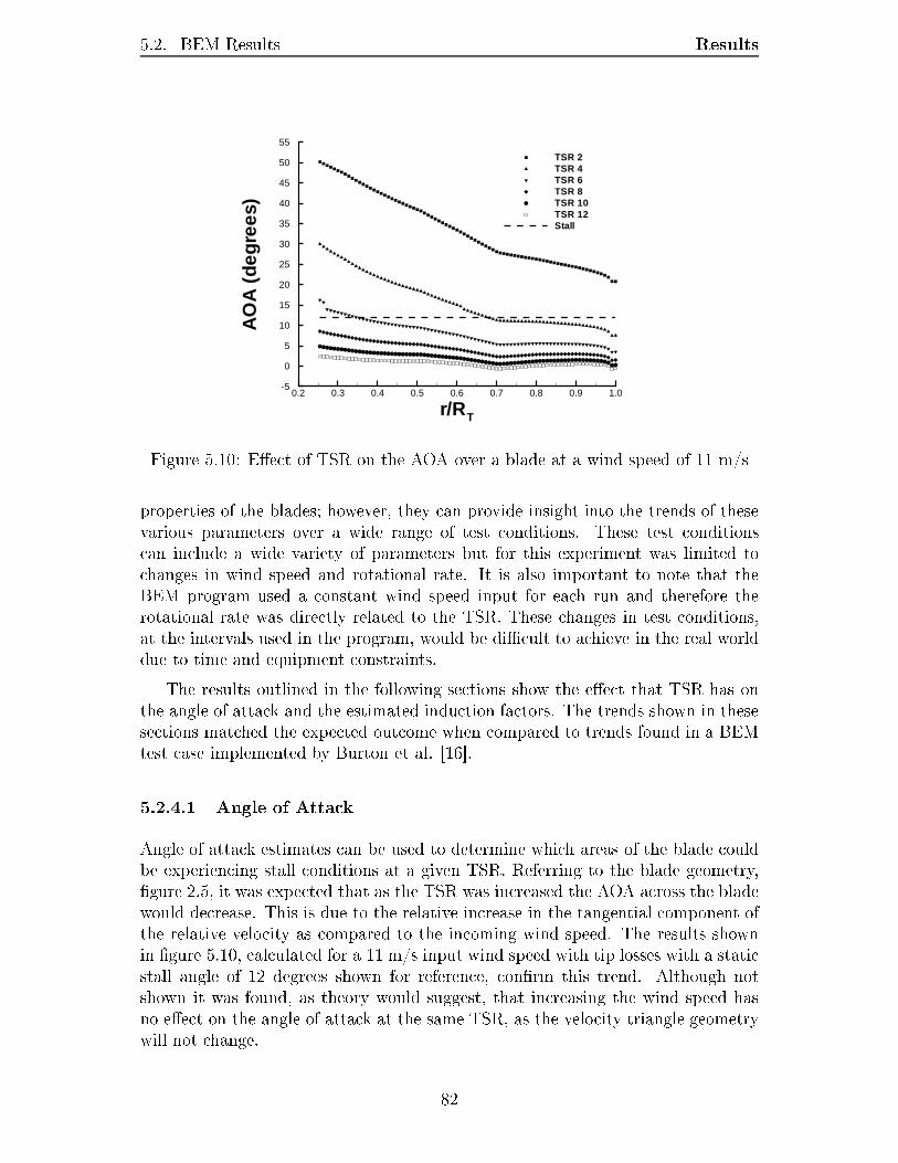
5.2. BEM Results Results

r/RT

AO

A(d

egre

es)

0.2 0.3 0.4 0.5 0.6 0.7 0.8 0.9 1.0-5

0

5

10

15

20

25

30

35

40

45

50

55

TSR 2TSR 4TSR 6TSR 8TSR 10TSR 12Stall

Figure 5.10: Eect of TSR on the AOA over a blade at a wind speed of 11 m/sproperties of the blades; however, they can provide insight into the trends of thesevarious parameters over a wide range of test conditions. These test conditionscan include a wide variety of parameters but for this experiment was limited tochanges in wind speed and rotational rate. It is also important to note that theBEM program used a constant wind speed input for each run and therefore therotational rate was directly related to the TSR. These changes in test conditions,at the intervals used in the program, would be dicult to achieve in the real worlddue to time and equipment constraints.The results outlined in the following sections show the eect that TSR has onthe angle of attack and the estimated induction factors. The trends shown in thesesections matched the expected outcome when compared to trends found in a BEMtest case implemented by Burton et al. [16].5.2.4.1 Angle of AttackAngle of attack estimates can be used to determine which areas of the blade couldbe experiencing stall conditions at a given TSR. Referring to the blade geometry,gure 2.5, it was expected that as the TSR was increased the AOA across the bladewould decrease. This is due to the relative increase in the tangential component ofthe relative velocity as compared to the incoming wind speed. The results shownin gure 5.10, calculated for a 11 m/s input wind speed with tip losses with a staticstall angle of 12 degrees shown for reference, conrm this trend. Although notshown it was found, as theory would suggest, that increasing the wind speed hasno eect on the angle of attack at the same TSR, as the velocity triangle geometrywill not change. 82

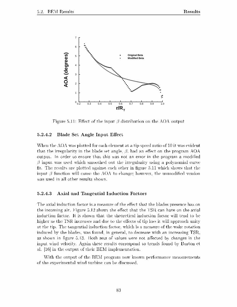
5.2. BEM Results Results

r/RT

AO

A(d

egre

es)

0.2 0.3 0.4 0.5 0.6 0.7 0.8 0.9 1.00

1

2

3

4

5

6

7

Original BetaModified Beta

Figure 5.11: Eect of the input β distribution on the AOA output5.2.4.2 Blade Set Angle Input EectWhen the AOA was plotted for each element at a tip speed ratio of 10 it was evidentthat the irregularity in the blade set angle, β, had an eect on the program AOAoutput. In order to ensure that this was not an error in the program a modiedβ input was used which smoothed out the irregularity using a polynomial curvet. The results are plotted against each other in gure 5.11 which shows that theinput β function will cause the AOA to change; however, the unmodied versionwas used in all other results shown.5.2.4.3 Axial and Tangential Induction FactorsThe axial induction factor is a measure of the eect that the blades presence has onthe incoming air. Figure 5.12 shows the eect that the TSR can have on the axialinduction factor. It is shown that the theoretical induction factor will tend to behigher as the TSR increases and due to the eects of tip loss it will approach unityat the tip. The tangential induction factor, which is a measure of the wake rotationinduced by the blades, was found, in general, to decrease with an increasing TSR,as shown in gure 5.13. Both sets of values were not aected by changes in theinput wind velocity. Again these results correspond to trends found by Burton etal. [16] in the output of their BEM implementation.With the output of the BEM program now known performance measurementsof the experimental wind turbine can be discussed.

83

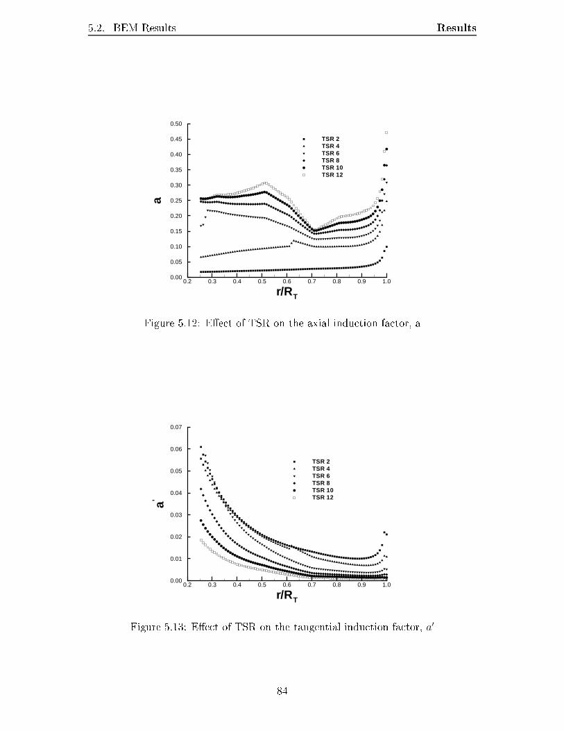
5.2. BEM Results Results

r/RT

a

0.2 0.3 0.4 0.5 0.6 0.7 0.8 0.9 1.00.00

0.05

0.10

0.15

0.20

0.25

0.30

0.35

0.40

0.45

0.50

TSR 2TSR 4TSR 6TSR 8TSR 10TSR 12

Figure 5.12: Eect of TSR on the axial induction factor, a

r/RT

a’

0.2 0.3 0.4 0.5 0.6 0.7 0.8 0.9 1.00.00

0.01

0.02

0.03

0.04

0.05

0.06

0.07

TSR 2TSR 4TSR 6TSR 8TSR 10TSR 12

Figure 5.13: Eect of TSR on the tangential induction factor, a′

84

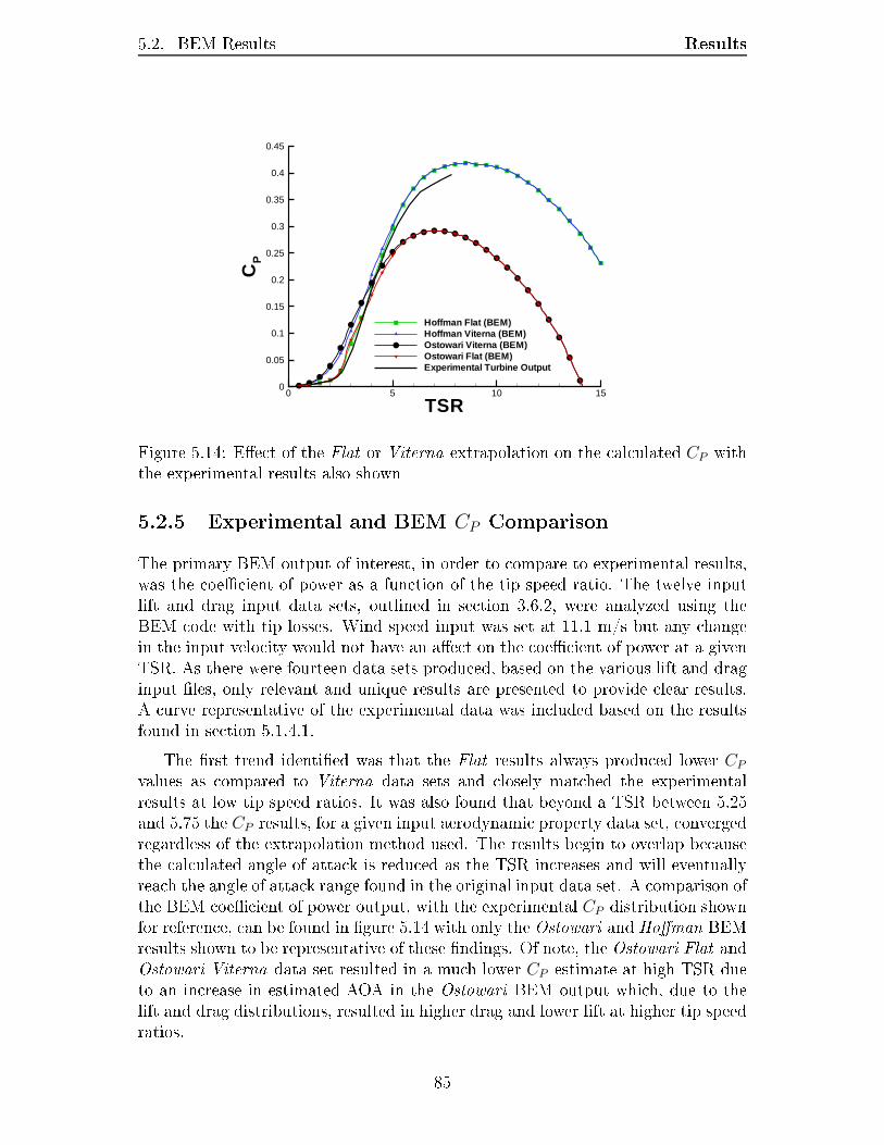
5.2. BEM Results Results

TSR

CP

0 5 10 150

0.05

0.1

0.15

0.2

0.25

0.3

0.35

0.4

0.45

Hoffman Flat (BEM)Hoffman Viterna (BEM)Ostowari Viterna (BEM)Ostowari Flat (BEM)Experimental Turbine Output

Figure 5.14: Eect of the Flat or Viterna extrapolation on the calculated CP withthe experimental results also shown5.2.5 Experimental and BEM CP ComparisonThe primary BEM output of interest, in order to compare to experimental results,was the coecient of power as a function of the tip speed ratio. The twelve inputlift and drag input data sets, outlined in section 3.6.2, were analyzed using theBEM code with tip losses. Wind speed input was set at 11.1 m/s but any changein the input velocity would not have an aect on the coecient of power at a givenTSR. As there were fourteen data sets produced, based on the various lift and draginput les, only relevant and unique results are presented to provide clear results.A curve representative of the experimental data was included based on the resultsfound in section 5.1.4.1.The rst trend identied was that the Flat results always produced lower CPvalues as compared to Viterna data sets and closely matched the experimentalresults at low tip speed ratios. It was also found that beyond a TSR between 5.25and 5.75 the CP results, for a given input aerodynamic property data set, convergedregardless of the extrapolation method used. The results begin to overlap becausethe calculated angle of attack is reduced as the TSR increases and will eventuallyreach the angle of attack range found in the original input data set. A comparison ofthe BEM coecient of power output, with the experimental CP distribution shownfor reference, can be found in gure 5.14 with only the Ostowari and Homan BEMresults shown to be representative of these ndings. Of note, the Ostowari Flat andOstowari Viterna data set resulted in a much lower CP estimate at high TSR dueto an increase in estimated AOA in the Ostowari BEM output which, due to thelift and drag distributions, resulted in higher drag and lower lift at higher tip speedratios. 85

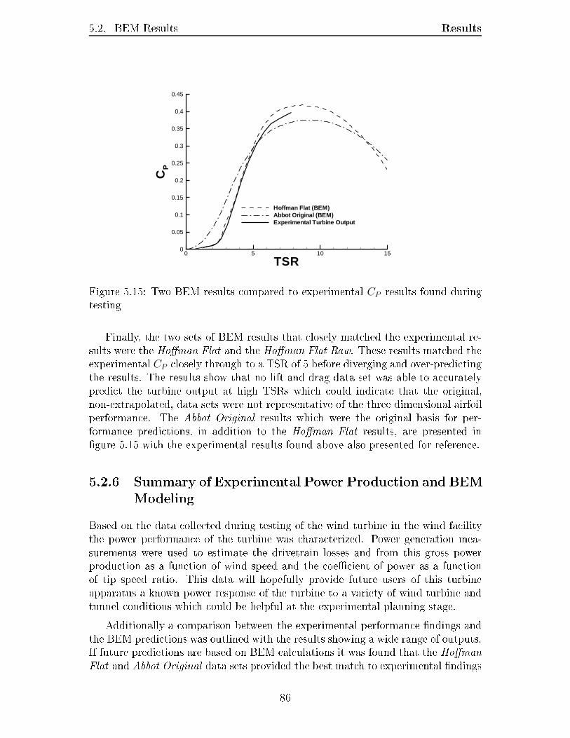
5.2. BEM Results Results

TSR

CP

0 5 10 150

0.05

0.1

0.15

0.2

0.25

0.3

0.35

0.4

0.45

Hoffman Flat (BEM)Abbot Original (BEM)Experimental Turbine Output

Figure 5.15: Two BEM results compared to experimental CP results found duringtestingFinally, the two sets of BEM results that closely matched the experimental re-sults were the Homan Flat and the Homan Flat Raw. These results matched theexperimental CP closely through to a TSR of 5 before diverging and over-predictingthe results. The results show that no lift and drag data set was able to accuratelypredict the turbine output at high TSRs which could indicate that the original,non-extrapolated, data sets were not representative of the three dimensional airfoilperformance. The Abbot Original results which were the original basis for per-formance predictions, in addition to the Homan Flat results, are presented ingure 5.15 with the experimental results found above also presented for reference.5.2.6 Summary of Experimental Power Production and BEMModelingBased on the data collected during testing of the wind turbine in the wind facilitythe power performance of the turbine was characterized. Power generation mea-surements were used to estimate the drivetrain losses and from this gross powerproduction as a function of wind speed and the coecient of power as a functionof tip speed ratio. This data will hopefully provide future users of this turbineapparatus a known power response of the turbine to a variety of wind turbine andtunnel conditions which could be helpful at the experimental planning stage.Additionally a comparison between the experimental performance ndings andthe BEM predictions was outlined with the results showing a wide range of outputs.If future predictions are based on BEM calculations it was found that the HomanFlat and Abbot Original data sets provided the best match to experimental ndings86

5.3. PIV Results Resultsin the current wind facility.5.3 PIV ResultsWith the experimental power ndings outlined above a discussion of the ow aroundthe turbine, as found using PIV, can now be made. The particle image velocimetryresults taken during testing have the potential to determine the nature of the owaround the blade at various turbine operational states. In total ve operationalstates were chosen for this portion of the experiment which represented three ex-pected tip speed ratios, 4, 6 and 8. The three tip speed ratios would be achievedwith three wind speed settings, 6.4, 7.5 and 11 m/s; and four rotational rates 111rpm, 167 rpm, 195 rpm and 220 rpm. The goal of the PIV testing was to determineif the PIV technique could resolve the ow conditions of an external ow over ablade at dierent tip speed ratios as well as those present at common tip speedratios.As shown in the BEM results the angle of attack of a blade element and coef-cient of power at a given tip speed ratio should remain constant. Experimentalresults given in section 5.1.4 conrm the coecient of power theory but PIV resultshad the potential to determine ow characteristics such as angle of attack at a pointalong the blade.After the data had been post processed, as outlined in section 4.3, averagedvelocity maps in the absolute reference frame could be produced. Additionally,ow parameters such as angle of attack could then be extracted from the relativevelocity vector map and streamlines could be produced to aid in the visualizationof the ow at the various operational states. Finally, repeatability between testdays and within data sets is discussed.5.3.1 Averaged Flow ResultsFrom the raw images captured during each test a vector map was produced, asdiscussed in section 4.3. Since each raw velocity correlation could not representthe ow within the entire imaging area it was necessary to average the acceptedvectors within each interrogation area to produce a complete vector map. Due tothe blade movement within the frame from one image to another the vector mapscould not be directly averaged without introducing additional error. As discussedin section 4.3, each image pair was correlated against a master image to determinethe relative position of the blade within the frame and shift the vector map tomatch. Both shifted and unshifted results are initially presented in this section todemonstrate the eect of the blades movement but in all subsequent discussionsthe shifted results were used.With the amount of shift determined for each image the corresponding PIV datacould be shifted to match. Figures 5.16 and 5.17 represent the unshifted and shifted87

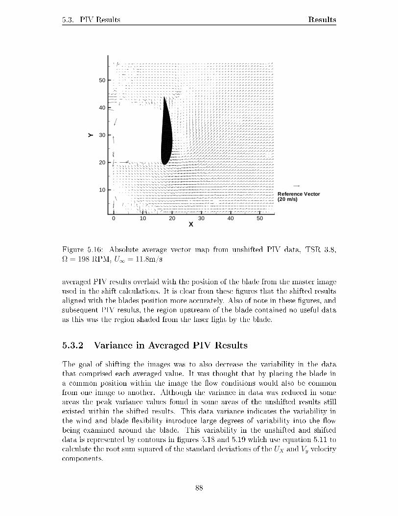
5.3. PIV Results Results

X

Y

0 10 20 30 40 50

10

20

30

40

50

Reference Vector(20 m/s)

Figure 5.16: Absolute average vector map from unshifted PIV data, TSR 3.8,Ω = 198 RPM, U∞ = 11.8m/saveraged PIV results overlaid with the position of the blade from the master imageused in the shift calculations. It is clear from these gures that the shifted resultsaligned with the blades position more accurately. Also of note in these gures, andsubsequent PIV results, the region upstream of the blade contained no useful dataas this was the region shaded from the laser light by the blade.5.3.2 Variance in Averaged PIV ResultsThe goal of shifting the images was to also decrease the variability in the datathat comprised each averaged value. It was thought that by placing the blade ina common position within the image the ow conditions would also be commonfrom one image to another. Although the variance in data was reduced in someareas the peak variance values found in some areas of the unshifted results stillexisted within the shifted results. This data variance indicates the variability inthe wind and blade exibility introduce large degrees of variability into the owbeing examined around the blade. This variability in the unshifted and shifteddata is represented by contours in gures 5.18 and 5.19 which use equation 5.11 tocalculate the root sum squared of the standard deviations of the UX and Vy velocitycomponents. 88

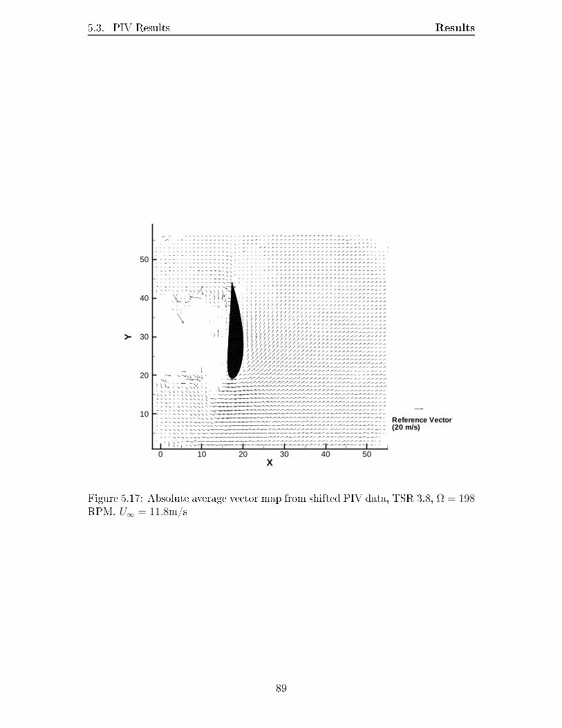
5.3. PIV Results Results

X

Y

0 10 20 30 40 50

10

20

30

40

50

Reference Vector(20 m/s)

Figure 5.17: Absolute average vector map from shifted PIV data, TSR 3.8, Ω = 198RPM, U∞ = 11.8m/s

89

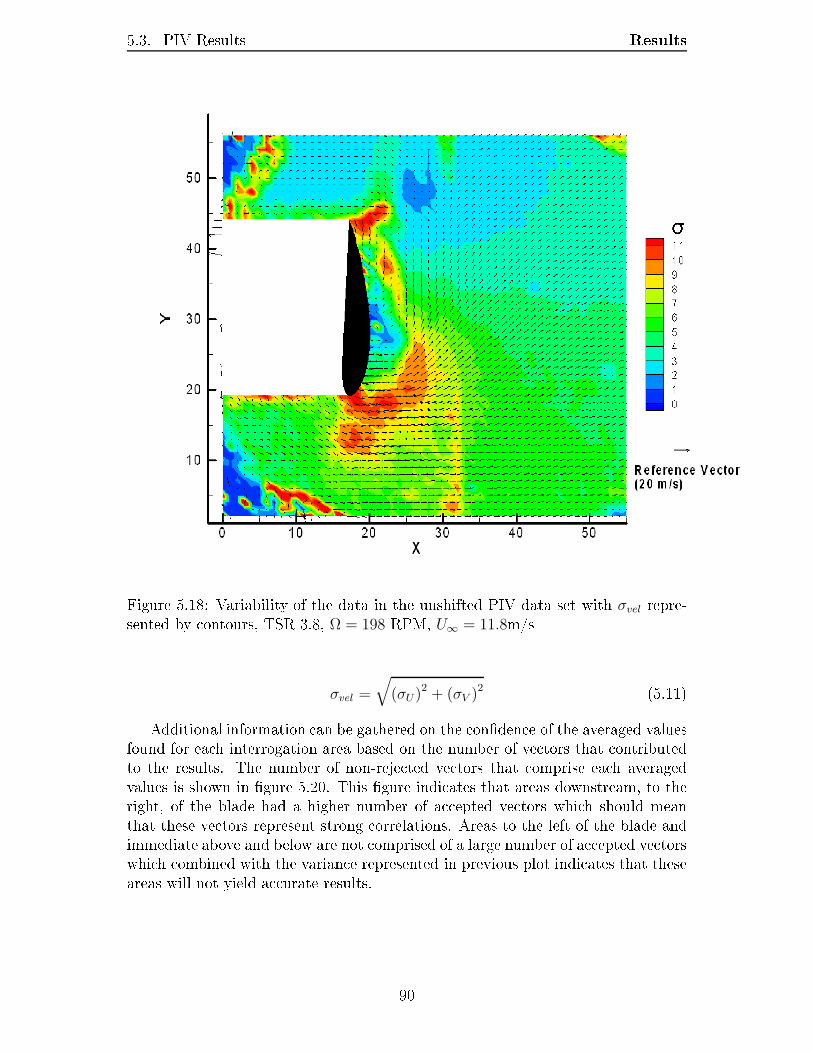
5.3. PIV Results Results

Figure 5.18: Variability of the data in the unshifted PIV data set with σvel repre-sented by contours, TSR 3.8, Ω = 198 RPM, U∞ = 11.8m/sσvel =

√

(σU)2 + (σV )2 (5.11)Additional information can be gathered on the condence of the averaged valuesfound for each interrogation area based on the number of vectors that contributedto the results. The number of non-rejected vectors that comprise each averagedvalues is shown in gure 5.20. This gure indicates that areas downstream, to theright, of the blade had a higher number of accepted vectors which should meanthat these vectors represent strong correlations. Areas to the left of the blade andimmediate above and below are not comprised of a large number of accepted vectorswhich combined with the variance represented in previous plot indicates that theseareas will not yield accurate results.90

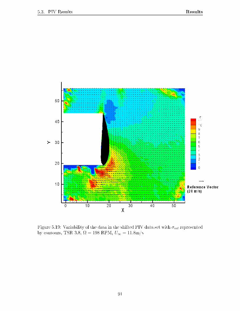
5.3. PIV Results Results

Figure 5.19: Variability of the data in the shifted PIV data set with σvel representedby contours, TSR 3.8, Ω = 198 RPM, U∞ = 11.8m/s

91

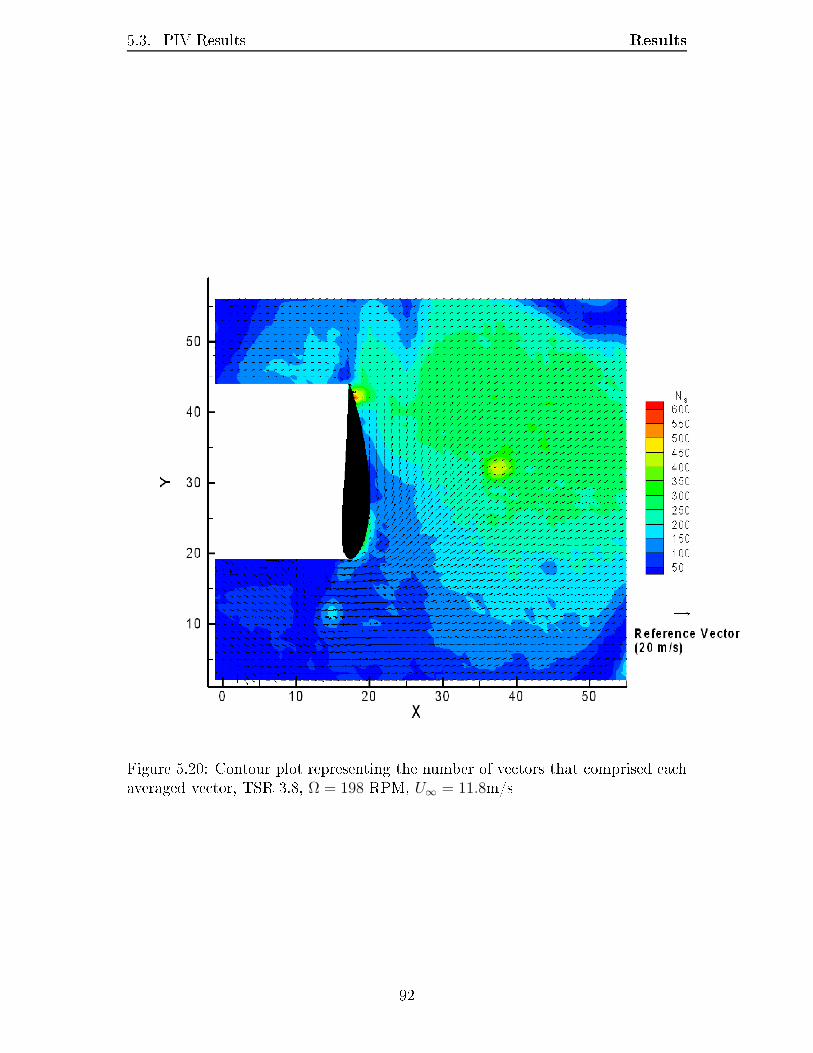
5.3. PIV Results Results

Figure 5.20: Contour plot representing the number of vectors that comprised eachaveraged vector, TSR 3.8, Ω = 198 RPM, U∞ = 11.8m/s

92

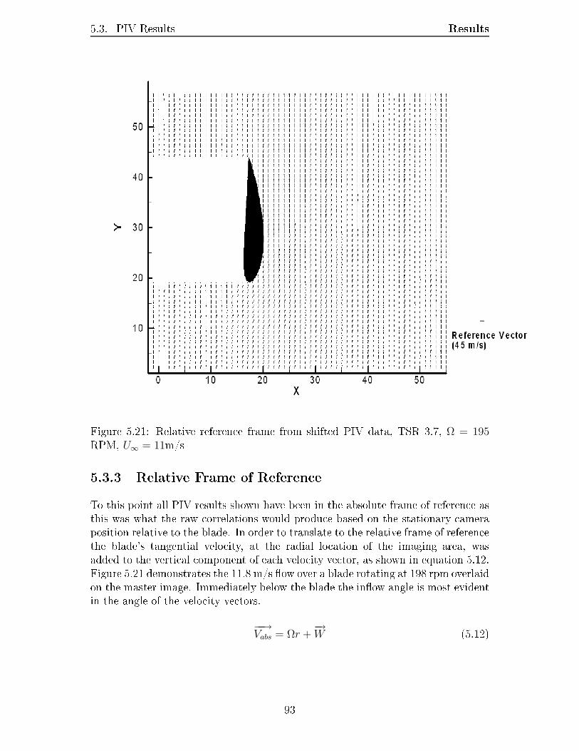
5.3. PIV Results Results

Figure 5.21: Relative reference frame from shifted PIV data, TSR 3.7, Ω = 195RPM, U∞ = 11m/s5.3.3 Relative Frame of ReferenceTo this point all PIV results shown have been in the absolute frame of reference asthis was what the raw correlations would produce based on the stationary cameraposition relative to the blade. In order to translate to the relative frame of referencethe blade's tangential velocity, at the radial location of the imaging area, wasadded to the vertical component of each velocity vector, as shown in equation 5.12.Figure 5.21 demonstrates the 11.8 m/s ow over a blade rotating at 198 rpm overlaidon the master image. Immediately below the blade the inow angle is most evidentin the angle of the velocity vectors.−−→Vabs = Ωr +

−→W (5.12)

93

5.3. PIV Results Results5.3.3.1 Angle of AttackIn the relative reference frame the angle of attack can also be found based on thevelocity triangle geometry. The velocity triangle denes the angle between therelative velocity and the tangential direction as the inow angle. From physicalmeasurements the blade set angle, β, was known at the radial location as 3.6degrees. With the inow and blade angle known the angle of attack could becalculated. Figure 5.22 shows the ow over the blade at a tip speed ratio of 3.8,11.8 m/s and rotational rate of 198 rpm, with the angle of attack shown by contoursand streamlines added to aid in the ow visualization. Testing completed at a tipspeed ratio of 3.7 under dierent input conditions, 6.8 m/s and 111 rpm, wascompleted to determine if the angle of attack would remain relatively constant asgiven by theory from the velocity triangle. The results of this second test at thesame tip speed ratio can be found in gure 5.23 which indicates that while theangle of attack is not identical in all interrogation areas the trends are similar.Additional testing completed at a tip speed ratio of 7.4, 6.8 m/s and 220 rpm,was expected to have an angle of attack approximately half that of those foundin the TSR 3.8 testing, based on the velocity triangle. The results found at thetip speed ratio of 7.4 are shown in gure 5.24 which does indicate a reduction inangle of attack in many areas except in large angles indicated near the leading andtrailing edges which were areas previously found to contain data that was suspectedto be less accurate.5.3.4 RepeatabilityThe repeatability of PIV results was a concern due to the high level of variabilityin the wind speed and to a certain degree the rotational rate of the turbine blade.In order to quantify the repeatability of PIV results two separate comparisons weremade: the rst between two separate tests on dierent days and the second compar-ison was made using two dierent sample sizes of the same velocity correlation datato comprise the averaged results. The rst test would determine if environmentalconditions on dierent days could aect the results. The second comparison woulddetermine the aect of the sample size on the results. Again the data sets usedwere from a tip speed ratio of 3.8, 11.8 m/s and 198 rpm, to represent the expectedworst case scenario for repeatability under high turbine loading.The full velocity correlation data from two dierent test days was shifted tothe master image location and averaged to produce vector maps, using techniquespreviously outlined. The results from the rst test were comprised of 769 corre-lations and the second test was comprised of 1027 correlations. The resulting Uand V components of the mean vector at each interrogation area were subtractedand the change in velocity was quantied as a percentage, given by equation 5.13.Results of this comparison can be found in gure 5.25 with red areas representingdata which was more that 100% dierent between the data sets and blue values94

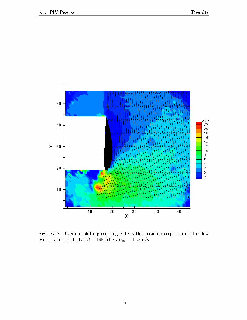
5.3. PIV Results Results

Figure 5.22: Contour plot representing AOA with streamlines representing the owover a blade, TSR 3.8, Ω = 198 RPM, U∞ = 11.8m/s

95

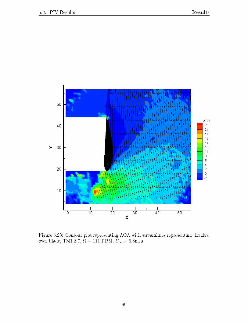
5.3. PIV Results Results

Figure 5.23: Contour plot representing AOA with streamlines representing the owover blade, TSR 3.7, Ω = 111 RPM, U∞ = 6.8m/s

96

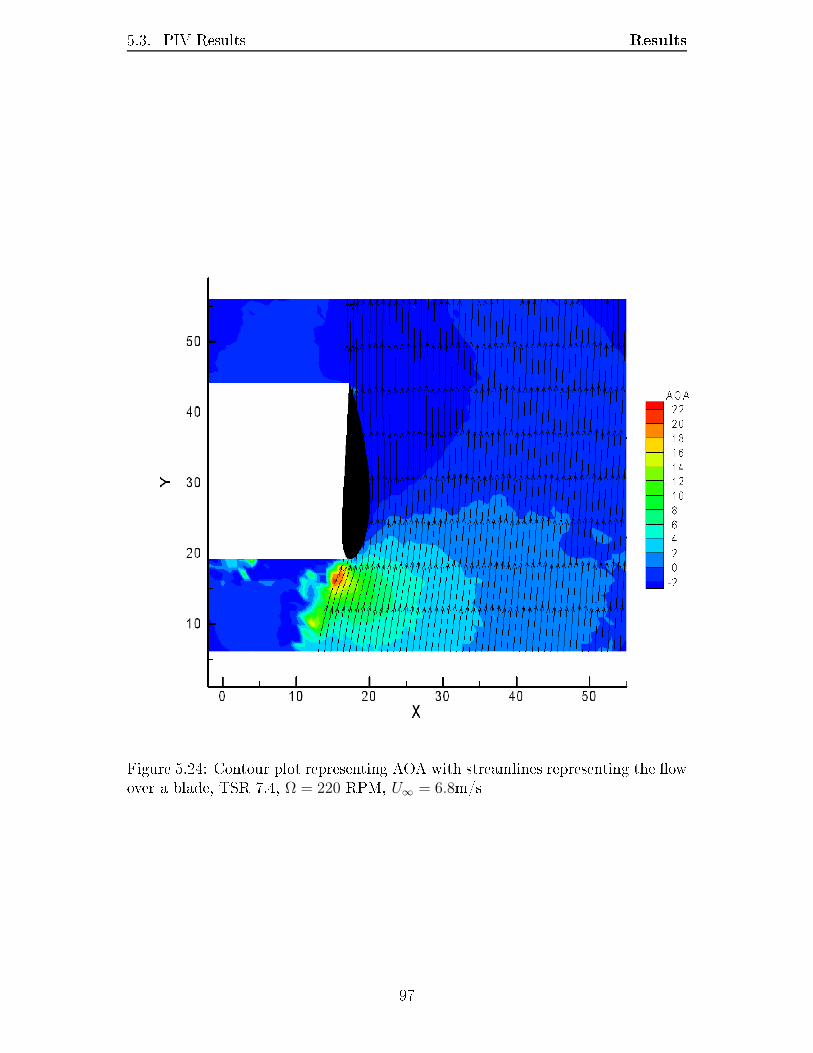
5.3. PIV Results Results

Figure 5.24: Contour plot representing AOA with streamlines representing the owover a blade, TSR 7.4, Ω = 220 RPM, U∞ = 6.8m/s

97

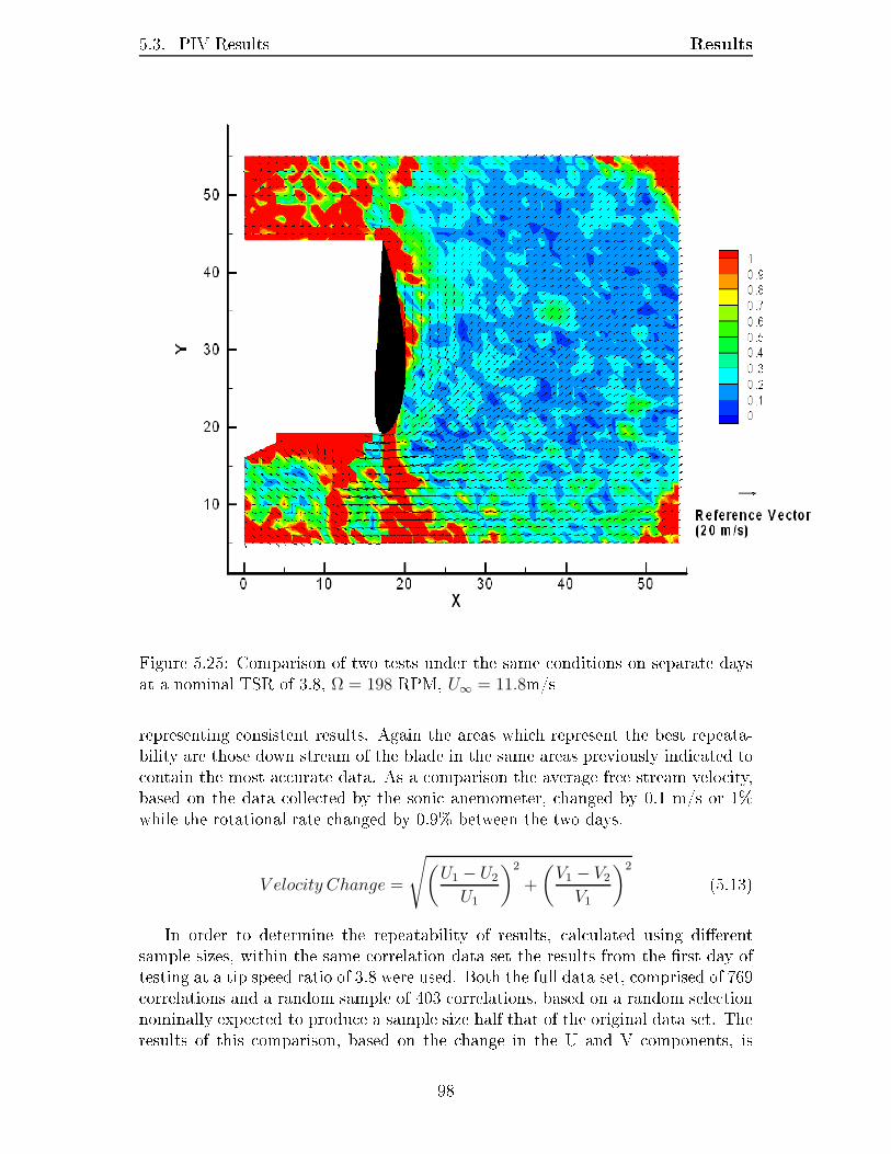
5.3. PIV Results Results

Figure 5.25: Comparison of two tests under the same conditions on separate daysat a nominal TSR of 3.8, Ω = 198 RPM, U∞ = 11.8m/srepresenting consistent results. Again the areas which represent the best repeata-bility are those down stream of the blade in the same areas previously indicated tocontain the most accurate data. As a comparison the average free stream velocity,based on the data collected by the sonic anemometer, changed by 0.1 m/s or 1%while the rotational rate changed by 0.9% between the two days.V elocity Change =

√

(

U1 − U2

U1

)2

+

(

V1 − V2

V1

)2 (5.13)In order to determine the repeatability of results, calculated using dierentsample sizes, within the same correlation data set the results from the rst day oftesting at a tip speed ratio of 3.8 were used. Both the full data set, comprised of 769correlations and a random sample of 403 correlations, based on a random selectionnominally expected to produce a sample size half that of the original data set. Theresults of this comparison, based on the change in the U and V components, is98

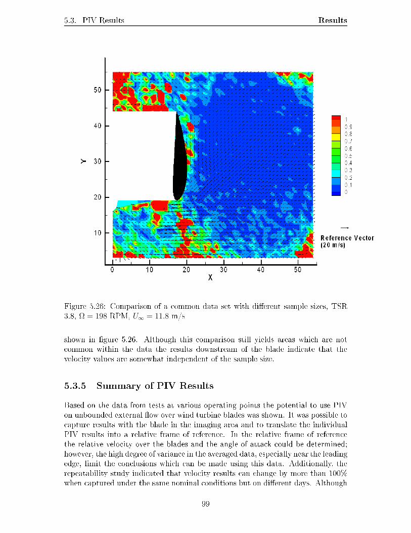
5.3. PIV Results Results

Figure 5.26: Comparison of a common data set with dierent sample sizes, TSR3.8, Ω = 198 RPM, U∞ = 11.8 m/sshown in gure 5.26. Although this comparison still yields areas which are notcommon within the data the results downstream of the blade indicate that thevelocity values are somewhat independent of the sample size.5.3.5 Summary of PIV ResultsBased on the data from tests at various operating points the potential to use PIVon unbounded external ow over wind turbine blades was shown. It was possible tocapture results with the blade in the imaging area and to translate the individualPIV results into a relative frame of reference. In the relative frame of referencethe relative velocity over the blades and the angle of attack could be determined;however, the high degree of variance in the averaged data, especially near the leadingedge, limit the conclusions which can be made using this data. Additionally, therepeatability study indicated that velocity results can change by more than 100%when captured under the same nominal conditions but on dierent days. Although99

5.3. PIV Results Resultsthe variance and repeatability indicate that improvements to the PIV technique,for this application, need to be made, as a proof of concept study the results areencouraging and represent the potential for further studies.

100

Chapter 6ConclusionsThe initial objectives of this project were to: measure the power output of a set ofturbine blades; evaluate BEM predictions against experimental data; and evaluatethe PIV technique for use in an unbounded rotational ow and if possible determinethe ow around a turbine blade. All of these goals were achieved and the resultswere presented in the previous chapter. Outlined below are the conclusions whichcan be drawn from the presented results. Additionally, improvements to the currentapparatus and future work which could be completed are also discussed.6.1 Wind Turbine Power ProductionWith basic power data from voltage and current measurements at the generatorand load bank the power production of the wind turbine was evaluated. Due to theability to vary both the incoming wind speed and the rotational rate a unique rangeof tip speed ratios could be evaluated. The raw power output was calculated as afunction of input wind velocity, peaking at 3080 W for a wind speed of 11.1 m/s.The eect of the tip speed ratio on the power coecient was also of interest as thisindicated the peak power production range for this particular turbine. While thetest apparatus was limited in it's rotational speed, and thus peak tip speed ratio,the peak coecient of power was approaching 40%.Although the variability in the wind facility free stream velocity was highthe power production results, specically in the non-dimensional power coecientcurve, demonstrate repeatability. This repeatability in the power measurementswas likely due to the inertia of the rotating turbine damping out the high frequencyvariation in the input wind speed.6.2 BEM PredictionsAs the results found in section 5.2.5 show the BEM prediction results are highlyvariable and dependent on the input airfoil aerodynamic properties. While some101

6.3. PIV ConclusionsBEM results were found to match experimental results at certain points in thepower curve, the variability between data sets conrmed the limited use theseresults can have for design purposes. However, it is a useful tool to determinetrends in parameters such as angle of attack and induction when evaluating theeects of dierent operating conditions involving combinations of wind speed androtational rate. If experimental time is limited this can help to determine whichoperating conditions should be tested to maximize the potential of the output data.For example if the objective of a test is to determine changes in the angle of attackalong a blade the rate of change of angle of attack is much higher at low tip speedratios than at higher tip speed ratios, as shown in gure 5.10, which could indicatemore testing would be required at low tip speed ratios to capture this rate of change.6.3 PIVThe experimental application of the PIV technique on the unbounded externalow over a rotating turbine blade presented unique challenges in addition to thetechnical challenges normally associated with the PIV technique. Despite thesechallenges, the PIV results presented show the potential to quantify the ow aroundthe blade and represented a unique application of the PIV technique; however,the movement of the blade within the imaging plane, primarily in the streamwisedirection, and the velocity uctuations in the free stream were likely the cause ofthe limited repeatability of the results. It was shown through post-processing ofthe images that the PIV results could be shifted to correspond to a common masterimage but this did not signicantly improve the variance in the data.The PIV results could be translated into a relative frame of reference which hadthe potential to extract inow angle, relative velocity and angle of attack values.Although the variance in the data did not allow a specic value to be found withany condence the technique was considered viable. Improvements to the tunnelow conditions and a reduction in turbine vibrations could allow PIV could be aviable technique in accurately quantifying the ow around this turbine. Althoughthe nal PIV results are only valid as a proof of concept they do represent a unique,and rst known, measurement of the ow eld over a rotating turbine blade.6.4 Equipment ImprovementsWhile the results found using the current equipment allowed power production andow measurements to be collected; inevitably, equipment improvements will allowan increased amount of unique data sets to be collected and analyzed. Improve-ments to: the structure of the nacelle, blades, wind facility, instrumentation andPIV equipment could all help to increase the accuracy and repeatability of theresults and allow a greater range of operating conditions to be tested.102

6.4. Equipment Improvements Conclusions6.4.1 Turbine and Blade AssemblyAs discussed previously the current turbine apparatus and blades do not allow forrotational rates beyond 220 RPM to be achieved without an excessive level of vibra-tion. This has been mostly attributed to the dynamic balance of the blade assemblyas the vibrations tend to increase with increasing rotational rate independent of anyinput wind from the fan banks. As the nacelle and tower structure were originallydesigned for a two bladed rotor with shorter blades installed more design analy-sis could be completed to help identify areas where structural improvements couldbe made to help reduce the potential for vibrations at common blade rotationalfrequencies which could be encountered during future tests.The blades themselves also experienced a noticeable amount of exing at thetip due to the loading at high wind speeds and rotational rates. This exing wasexpected but likely added to the variability of the PIV results near the tip of theblade. While nothing can be done to improve the structure of the existing bladesmitigating this exibility in future blade designs would likely improve any resultswhether they are power, pressure or PIV based. To this end the MEXICO project[6] used milled aluminum blades for all testing to help improve the stiness of theblades and thus the repeatability of their tests which could be used as a model forfuture experimental blade structure.Signicant improvements could also be made to the rotational speed control ofthe blades. Currently this control is manual and relies on the operator trackingthe speed of the rotor with a computer readout and adjusting the input voltage tothe eld and armature to achieve the desired rotational rate. Ideally this would beaccomplished automatically with an electronic speed controller which would allowthe operator to have greater control over the speed of the rotor. Alternatively, orin conjunction with a speed controller, greater control over the turbine loading,currently in the form of a xed resistance load bank, could be achieved using avariable resistive load. As the load bank currently has a xed resistance it mustbe able to absorb the maximum expected power output of the turbine for anygiven test. With a variable resistive load on the turbine the power absorbed by theload bank could be dynamically altered to provide speed control to the turbine,essentially acting as an electric braking system.6.4.2 Wind FacilityThe wind tunnel streamwise velocity characteristics, outline in section 3.2.1, in-dicated that there was a high level of turbulence present in the ow which wasalso observed during PIV testing in the smoke particle stream motion. This tur-bulence was seen as one of the leading contributors to the challenges encounteredwhile attempting PIV measurements on the blades and ultimately to the limitedrepeatability of the PIV results. While this facility will likely not achieve very lowturbulence levels often found in purpose built wind tunnels, improvements to the103

6.4. Equipment Improvements Conclusionsfacility and the layout could improve the ow conditions for wind turbine testing.These improvements could include, but are not limited to, the ow straighteningsection of the facility, fan outlets and moving semi-permanent objects which cur-rently obstruct the ow path.6.4.3 InstrumentationWhile current instrumentation allows the power into and out of the generator tobe measured the power produced by the blades can only be estimated from thesemeasurements. A torque sensor placed on the low speed shaft, combined withan improved rotational rate sensor, would provide a more accurate measurementof the torque and power that the blades are producing. Additionally pressuresensors on the blades and load cells attached to each blade could help to providemore information on the individual blade loading. As blade pressure and loadmeasurements were made during the NREL [5] and MEXICO [6] studies; futuretesting, with the current apparatus, which incorporated similar sensors could onlyimprove the condence in the results and conclusions.6.4.4 PIV EquipmentFinally, improvements to the PIV equipment will help to gain a better under-standing of the complex ow which is present around a turbine blade. Based oncurrent results the improvements, outlined above, to the tunnel and turbine as-sembly should be made in order to improve the repeatability and quality of thePIV results. If these improvements are made the camera and laser used to capturethe images could then be upgraded. These upgrades would primarily involve thespeed at which images are captured which can ultimately lead to time-resolved PIVimages. Time-resolved PIV would be able to capture any transient eects as theblade moves through the imaging plane.Movement of the camera and laser sheet to various radial locations along theblade as well as traversing upstream and downstream of the blade would be thenext logical step in PIV experimentation on this apparatus. Imaging at dierentpoints along the blade would provide insight into the ow patterns closer to theroot of the blade. Additionally imaging completed upstream and downstream ofthe rotor plane would allow the aect of the rotors presence on the free stream to bequantied. These tests would be similar to the MEXICO project goals and results[15] and could yield PIV based measurements of parameters such as the axial andtangential induction factors.104

6.5. Recommendations for Future Research Projects Conclusions6.5 Recommendations for Future Research ProjectsIn most experimental studies more work can be done and further analysis of theresulting data is likely possible. The equipment improvements outlined above listsome of the limitations of the current experimental apparatus and some of theimprovements which can be made to rectify those limitations. With the relevantequipment improvements in place the potential for future research projects study-ing power production and blade ow aerodynamics are endless. Research projectsrelated to power production, BEM modeling and PIV are proposed below.6.5.1 Power Production StudiesSome future studies which could yield interesting power production results for ex-amination could include: dierent blade congurations, yawed rotor plane, higherwind speeds and rotational rates and thus a wider range of tip speed ratios. Customblade congurations would allow studies which could determine the eects of: tipdesign, surface roughness or twist distributions on the power production. Basedon the previous studies by NREL and MEXICO, as outlined in section 2.1, thepower production of a wind turbine in yawed conditions is of interest to the windturbine research community. Finally, testing conducted over a wider range of tipspeed ratios will allow the peak power to be determine for the current rotor designas current limitations on wind speed and rotational rates were a limiting factor fortesting. Overall the exibility inherent in the design of the turbine structure andthe electrical system should yield useful data through a wide range of applications.6.5.2 BEM Model StudiesThe inability of the basic BEM model, implemented for this study, to accuratelypredict the output of the wind turbine's experimental power output demonstrateda need for an improved model. For future experiments an approximation of theturbine performance and loading will be useful if dierent blade designs or operat-ing conditions are studied. With the experimental power production of the currentturbine conguration now known it may be possible to adjust the model input pa-rameters such as the tip loss factor or aerodynamic lift and drag curves to improvethe correlation to the experimental data. Studies could also be completed deter-mine the eect of dividing the blades into dierent airfoils instead of the currentimplementation which assumes the blade can be represented by a single NACAprole. Additionally, implementing advanced models which attempt to account forthree dimensional eects and wake ow conditions could help to improve the ac-curacy of the predictions, although even advanced models struggle to consistentlypredict turbine output, as discussed in section 2.1.1.3.105

6.5. Recommendations for Future Research Projects Conclusions6.5.3 PIV StudiesThe PIV experimentation shows promise for further study due to the unique ap-plication of the technique when used to measure the ow around the blades. Ifthe issues related to seeding and free stream turbulence are solved studies relatedto the ow in and around the blade and rotor plane would yield unique resultsand data for the wind turbine research community. Specic areas of research couldinclude: chordwise ow measurements captured at various radial locations; mea-suring span wise (radial) ow which may be present during some operation points;nally, placement of the camera in the rotating domain to allow image capture atvarious azimuth points and to allow time resolved PIV measurements of the bladeow.

106

References[1] Abbot, Ira H. and Albert E. Von Doenho, Theory of Wing Sections. DoverPublications Inc., New York, NY, 1959. iii, xiii, 35, 37, 39, 40[2] Homan, M. J., R.R. Ramsay and G.M. Gregorek, Eects of Grit Roughnessand Pitch Oscillations on the NACA 4415 Airfoil. Tech. Rep. NREL/TP-442-7815, NREL, Golden, Colorado, July 1996. iii, xiii, 35, 38, 39, 40[3] IEA Wind Energy Annual Report 2007. Tech. rep., IEA Wind, July 2008. 1[4] Energy Statistics Handbook: Fourth Quarter 2008. Tech. Rep. 57-601-X2008004, Statistics Canada, May 2009. 1[5] Hand, M. M., D. A. Simms, L. J. Fingersh, D. W. Jager, J. R. Cotrell,S. Schreck and S. M. Larwood, Unsteady Aerodynamics Experiment Phase VI:Wind Tunnel Test Congurations and Available Data Campaigns. Tech. Rep.NREL/TP-500-29955, NREL, December 2001. xi, 4, 5, 7, 104[6] Schepers, J. G. and H. Snel, Model Experiments in Controlled Conditions:Final Report. Tech. Rep. ECN-E07-042, ECN, June 2007. xi, xii, 4, 9, 10, 11,12, 20, 103, 104[7] Somers, D. M., Design and Experimental results for the S809 Airfoil. Tech.Rep. NREL/SR-440-6918, Airfoils Inc. for NREL, January 1997. 5[8] Schreck, Scott, The NREL Full-Scale Wind Tunnel Experiment: Introductionto the Special Issue. Wind Energy, 5:7784, 2002. xii, 6[9] Schepers, J. G. and R.P.J.O.M. van Rooij, Analysis of aerodynamic measure-ments on a model wind turbine placed in the NASA-Ames tunnel: ECN's andTUD's contribution to IEA Wind Task XX. Tech. Rep. ECN-E08-052, ECN,2008. xii, 7[10] Simms, D., S. Schreck, M. Hand and L. J. Fingersh, NREL Unsteady Aerody-namics Experiment in the NASA-Ames Wind Tunnel: A Comparison of thePredictions to Measurements. Tech. Rep. NREL/TP-500-29494, NREL, 2001.8 107

References REFERENCES[11] Coton, Frank N., Tongguang Wang and Roderic A McD. Galbraith, An Ex-amination of Key Aerodynamic Modelling Issues Raised by the NREL BlindComparison. Wind Energy, 5:199212, 2002. 8[12] Breton, Simon-Philippe, Frank N. Coton and Geir Moe, A Study on Rota-tional Eects and Dierent Stall Delay Models Using a Prescribed Wake Vor-tex Scheme and NREL Phase VI Experiment Data. Wind Energy, 11:459482,2008. 8[13] Laino, David J., A. Craig Hansen and Je E. Minnema, Validation of theAeroDyn Subroutines Using NREL Unsteady Aerodynamics Experiment Data.Wind Energy, 5:227244, 2002. 8[14] Schreck, Scott J., Niels N. Sorensen and Michael C. Robinson, AerodynamicStructures and Processes in Rotationally Augmented Flow Fields. Wind Energy,10:159178, 2007. 9[15] Snel, H., J.G. Schepers and B. Montgomerie, The MEXICO project (ModelExperiments in Controlled Conditions): The database and rst results of dataprocessing and interpretation. Journal of Physics: Conference Series The Sci-ence of Making Torque from Wind, 75:111, 2007. xii, 9, 11, 12, 20, 104[16] Burton, Tony, David Sharpe, Nick Jenkins and Ervin Bossanyi, Wind EnergyHandbook. John Wiley and Sons Canada Ltd., 2006. xv, 13, 15, 82, 83, 111,112[17] The Mathworks Inc., Matlab. xi, 14, 62, 66, 113[18] Martinez, Jaime, Luca Bernabini, Oliver Probst and Ciro Rodriguez, An Im-proved BEM Model for the Power Curve Prediction of Stall-regulated WindTurbines. Wind Energy, 8:385402, 2005. 16[19] Glauert, H., 'Airplane Propellers', Aerodynamic Theory: A General Reviewof Progress, vol. IV. (ed. William Frederick Durand), Dover Publications Inc.,New York, 1963. 16[20] Shen, Wen Zhong, Robert Mikkelsen and Jens Norkaer Sorensen, Tip Losscorrections for Wind Turbine Computations. Wind Energy, 8:457475, 2005.16[21] Dantec Dynamics Inc., FlowMap Particle Image Velocimetry Instrumentation:Installation and User's Guide, 1999. 18, 60[22] Melling, A, Tracer particles and seeding for particle image velocimetry. Mea-surement Science Technology, 8:14061416, 1997. 18[23] New Wave Research, Solo PIV Nd:YAG Laser System Operator's Manual,April 2006. 19, 42, 60 108

References REFERENCES[24] Particle Image Velocimetry (PIV) Principles. Dantec Dynamic Inc., May 2009,http://www.dantecdynamics.com/. xii, 19[25] Altaf, Ammar Mohammadnour, Experimental Investigation of the Flow Be-haviour Inside a Centrifugal Impeller Channel at Design and O-Design FlowRates. Master's thesis, University of Waterloo, 2007. 19[26] Sante, Alberto Di, Raf Theunissen and Rene A. Van den Braembussche, A newfacility for time-resolved PIV measurements in rotating channels. ExperimentalFluids, 44:179188, 2008. 19[27] Ferreira, Carlos Simao, Gijs van Kuik, Gerard van Sussel and Fulvio Scarano,Visualization by PIV of dynamic stall on a vertical axis wind turbine. Experi-mental Fluids, 46:97108, 2009. 20[28] McWilliam, Michael K., Development of a Wind Turbine Test Apparatus forHorizontal Axis Wind Turbine Rotor Testing. Master's thesis, University ofWaterloo, Waterloo, ON, 2008. xii, 21, 25, 26, 30[29] Johnson, David, Wind Energy Laboratory. University of Waterloo, De-partment of Mechanical and Mechatronics Engineering, September 2006,http://www.mme.uwaterloo.ca/~da3johns/johnfacility.html. 21[30] Wraith, Chris, Personal Correspondence. Composotech Structures Inc., 2007-2008, http://www.composotech.com. 30, 124, 126, 127[31] Whisper 500. Southwest Windpower Inc, February 2007,http://www.windpower.com/products/whisper_500.htm. 30[32] SolidWorks Corporation, SolidWorks, 2006. 32[33] Trapp, Jens and Robert Zores, NACA 4 Digit series, April 2008,http://www.pagendarm.de/trapp/programming/java/profiles/NACA4.html.34[34] Ostowari, C. and D. Naik, Post Stall Studies of Untwisted Varying AspectRatio Blades with an NACA 4415 Airfoil Section - Part I. Wind Engineering,8(3):176194, 1984. xiii, 35, 38, 39, 40, 41[35] Drela, Mark and Harold Youngren, Xfoil 6.96, 2006,http://web.mit.edu/drela/Public/web/xfoil/. xiii, 35, 38, 39, 40[36] Hansen, Craig, NWTC Design Codes: AirfoilPrep, January 2007,http://wind.nrel.gov/designcodes/preprocessors/airfoilprep/. 35[37] Viterna, L.A. and D.C. Janetzke, Theoretical and Experimental Power fromLarge Horizontal-Axis Wind Turbines. Tech. Rep. NASA TM-82944, NASA,September 1982. 36 109

References REFERENCES[38] Moriarty, Patrick J. and A. Craig Hansen, AeroDyn Theory Manual. Tech.Rep. NREL/EL-500-36881, National Renewable Energy Laboratory, Colorado,December 2005. 36[39] Laino, David J. and A. Craig Hansen, User's Guide to the Wind Turbine Aero-dynamics Computer software: AeroDyn. Windward Engineering, Salt LakeCity, Utah, 12.50 ed., December 2002. 36[40] Dantec Dynamics Inc., FlowManager, 1999. 41, 137[41] National Instruments Corp, Kodak Megaplus ES 1.0 Camera Manual. 372259a-01 ed., November 1998. 42, 60[42] Keithley Instruments Inc., Model 2700 Multimeter/Switch System User's Man-ual, 2001. xi, 48, 49, 118[43] National Instruments Corp., NI 6251 Specications. 371291h-01 ed., 2007. 48,119[44] Campbell Scientic Canada Corp, 3-D Sonic Anemometer User Manual, 2004.48[45] National Instruments Corp., Labview. vii, 50[46] Holman, J.P., Experimental Methods for Engineers. McGraw Hill, Toronto,1966. 63, 71[47] Moat, Robert J., Describing the Uncertainties in Experimental Results. Ex-perimental Thermal and Fluid Science, 1:317, 1988. 116[48] Seglenieks, Frank, Waterloo Weather Station. University of Water-loo, Department of Civil and Environmental Engineering, 2008,http://weather.uwaterloo.ca. 120[49] CoREZYN COR61-AA-340 Resin. Interplastic Corporation: ThermosetResins Division, http://www.interplastic.com/corezyn_TR.html. 126[50] Hydrophilic Amorphous Fumed SIlica: HC0043040. Wacker Chemie AG,http://www.wacker.com. 126[51] Econostitch 5445 Data Sheet. Tech. rep., Airtech Advanced Materials Group,Huntington Beach, CA, November 2008, www.peelply.com. 130110

Appendix ABEMA.1 Betz Limit DerivationThe BEM theory, as the name implies, was based on a momentum analysis of arotor which is modeled as a momentum sink. This rotor will decrease the streamwisevelocity along a streamtube and have a sharp pressure drop across the rotor plane,as shown in gure A.1 from Burton et al. [16]. A streamwise momentum analysiswill yield equation A.3 based on the terms outlined in gure A.1 and the denitionof the axial induction factor found in equation A.1.[16]

a =U∞ − Ud

U∞

(A.1)∑

Fx =(

P+d − P−

d

)

Ad = (U∞ − UW ) ρAdUd (A.2)∑

Fx =(

P+d − P−

d

)

Ad = (U∞ − UW ) ρAdU∞ (1 − a) (A.3)The Bernoulli equation was then used to determine a relationship, found inequation A.6, between the pressure dierence across the rotor plane and the airvelocity upstream and downstream of the turbine.1

2ρU2

∞+ P∞ =

1

2ρU2

d + P+d (A.4)

1

2ρU2

W + P∞=1

2ρU2

d + P−

d (A.5)P+

d − P−

d =1

2ρ

(

U2∞− U2

W

) (A.6)111

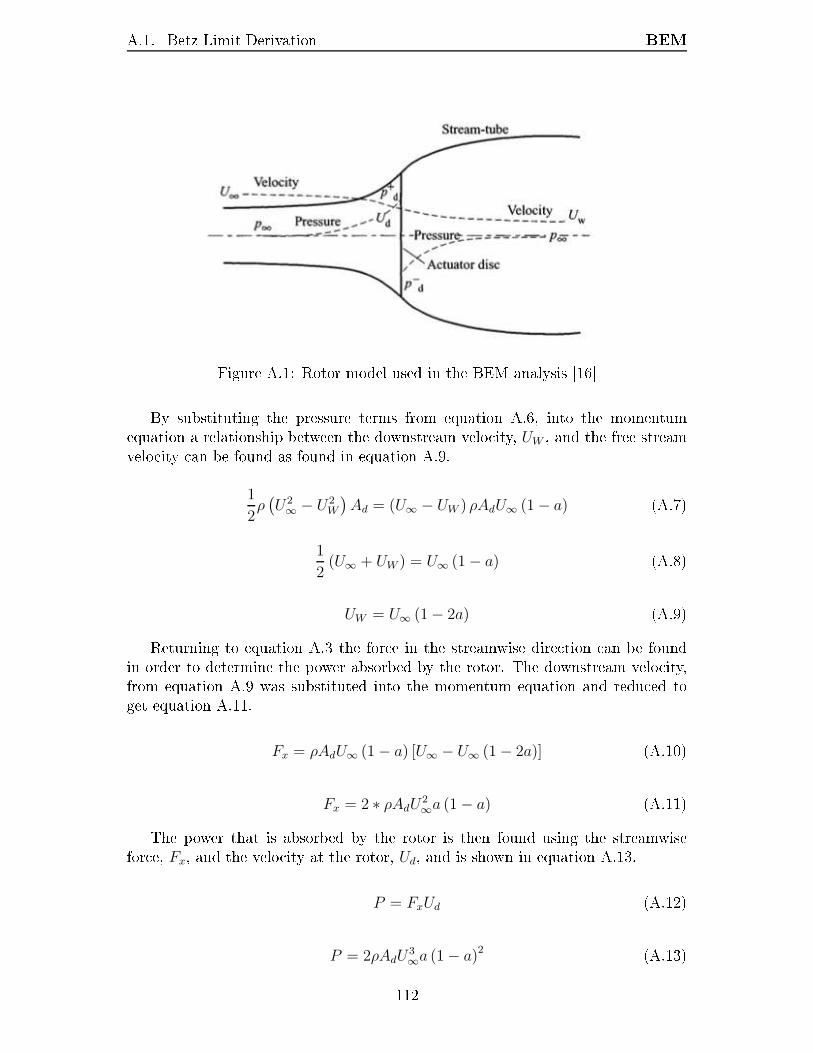
A.1. Betz Limit Derivation BEM

Figure A.1: Rotor model used in the BEM analysis [16]By substituting the pressure terms from equation A.6, into the momentumequation a relationship between the downstream velocity, UW , and the free streamvelocity can be found as found in equation A.9.1

2ρ

(

U2∞− U2

W

)

Ad = (U∞ − UW ) ρAdU∞ (1 − a) (A.7)1

2(U∞ + UW ) = U∞ (1 − a) (A.8)

UW = U∞ (1 − 2a) (A.9)Returning to equation A.3 the force in the streamwise direction can be foundin order to determine the power absorbed by the rotor. The downstream velocity,from equation A.9 was substituted into the momentum equation and reduced toget equation A.11.Fx = ρAdU∞ (1 − a) [U∞ − U∞ (1 − 2a)] (A.10)

Fx = 2 ∗ ρAdU2∞

a (1 − a) (A.11)The power that is absorbed by the rotor is then found using the streamwiseforce, Fx, and the velocity at the rotor, Ud, and is shown in equation A.13.P = FxUd (A.12)

P = 2ρAdU3∞

a (1 − a)2 (A.13)112

A.2. BEM Matlab Code BEMThe coecient of power can then be found, as dened by equation A.14, usingthe power derived above. The coecient of power based on this momentum analysis,is shown in equation A.16, was found to only be a function of the axial inductionfactor.CP =

P12ρAdU3

∞

(A.14)CP =

2ρAdU3∞

a (1 − a)2

12ρAdU3

∞

(A.15)CP = 4a (1 − a)2 (A.16)The maximum coecient of power was then determined by dierentiating equa-tion A.16 with respect to the axial induction factor. The maximum power coecientwas found to be 59.3% at an induction factor of 1/3 and is referred to as the Betzlimit.A.2 BEM Matlab CodeOutlined below is the code used to implement the BEM theory in Matlab [17].clear ;close a l l ;t ic%Air fo i l parameters found from actual bladeR_t=2.1735; %metresN=3; % number of b ladesex c l =0.246719; %amount to exclude , hub areau_inf =11.13; %free stream ve l oc i t y (m/s )rho =1.2 ; %density (kg/m^3)%use ' chord (r_rat) ' function to get chord at r/R value%use ' setangle (r_rat , exc l ) ' function to get beta at r/R value%use ' force ( alpha ) ' to get c l and cd at angle of attack in degrees%choose number of elements to divide bladeelem=110;m=1; %in i t i a l i z e t ip speed i tera t ion counterfor k=0 .1 : 0 . 1 : 1 5lamda_t=k ;%in i t i a l i z e arraysphi=zeros (1 ) ;beta_val=zeros (1 ) ;alpha=zeros (1 ) ;sigma=zeros (1 ) ;c l=zeros (1 ) ;cd=zeros (1 ) ;a=zeros (1 ) ;a_prime=zeros (1 ) ;f a c t o r=zeros (1 ) ;F=zeros (1 ) ;%in i t i a l i z e t o t a l valuesT=0;Th=0;P=0;%find i n i t i a l va lues based on optimum rotorfor i =1:elemr_rat=i / elem ;lamda (1 , i )=lamda_t∗ r_rat ; %element speed rat ioa (1 , i ) =1/3;a_prime (1 , i )=0; 113

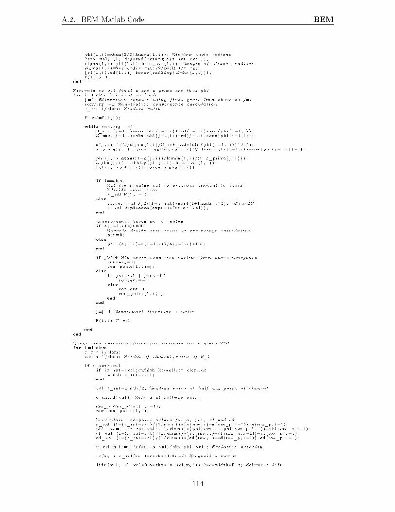
A.2. BEM Matlab Code BEMphi (1 , i )=atan(2/3/ lamda (1 , i ) ) ; %inf low angle , radiansbeta_val (1 , i )=deg2rad ( s e t ang l e ( r_rat , e xc l ) ) ;alpha (1 , i )=phi (1 , i )−beta_val (1 , i ) ; %angle of attack , radianssigma (1 , i )=N∗ chord ( r_rat ) /2/pi /R_t/ r_rat ;[ c l ( 1 , i ) ,cd (1 , i ) ]= f o r c e ( rad2deg ( alpha (1 , i ) ) ) ;F(1 , i )=1;end%it e ra t e to get f i n a l a and a_prime and thus phifor i =1:elem %element on bladej =2; %itera t ion counter using f i r s t guess from above as j=1converg=−1; %in i t i a l i z e convergence ca lcu la t ionr_rat=i / elem ; %radius ra t ioF_val=F(1 , i ) ;while converg==−1C_n=c l ( j −1, i )∗cos ( phi ( j −1, i ) )+cd ( j −1, i )∗ sin ( phi ( j −1, i ) ) ;C_t=c l ( j −1, i )∗ sin ( phi ( j −1, i ) )−cd ( j −1, i )∗cos ( phi ( j −1, i ) ) ;a ( j , i ) =1/(4/ sigma (1 , i ) /C_n∗F_val∗( sin ( phi ( j −1, i ) ) )^2+1) ;a_prime ( j , i )=1/(4∗F_val/ sigma (1 , i ) /C_t∗ sin ( phi ( j −1, i ) )∗cos ( phi ( j −1, i ) )−1) ;phi ( j , i )=atan((1−a ( j , i ) ) / lamda (1 , i ) /(1+a_prime ( j , i ) ) ) ;alpha ( j , i )=rad2deg ( phi ( j , i )−beta_val (1 , i ) ) ;[ c l ( j , i ) ,cd ( j , i ) ]= f o r c e ( alpha ( j , i ) ) ;i f i==elem%at t ip F value se t to previous element to avoid%divide zero errorF_val=F(1 , i −1) ;else f a c to r_va l=N/2∗(1− r_rat )∗sqrt (1+lamda_t^2) ; %PrandtlF_val=2/pi∗acos (exp(−1∗ f a c to r_va l ) ) ;end%convergence based on 'a ' valuei f a ( j −1, i ) <0.0001%avoids divide zero error in percentage ca lcu la t ionper=0;else per=(a ( j , i )−a ( j −1, i ) ) /a ( j −1, i ) ∗100;endi f j >100 %to avoid excessive runtime from non−convergenceconverg =1;con_point (1 , i )=j ;else i f per >0.1 | per <−0.1converg=−1;else converg =1;con_point (1 , i )=j ;endendj=j +1; %increment i tera t ion counterF(1 , i )=F_val ;endend%loop used ca lcu la te force for elements for a given TSRfor i =1:elemr_rat=i / elem ;width=1/elem ; %width of element , ra t io of R_ti f r_rat>ex c li f ( r_rat−e xc l )<width %smal lest elementwidth=r_rat−e xc l ;endval=r_rat−width /2 ; %radius ra t io at ha l f way point of elementc=chord ( val ) ; %chord at halfway pointrow_p=con_point (1 , i −1) ;row=con_point (1 , i ) ;%calcu la te mid−point values for a , phi , c l and cda_val=(1−(r_rat−val ) /(1/ elem ) ) ∗(a ( row , i )−a (row_p , i −1) )+a (row_p , i −1) ;phi_val=(1−(r_rat−val ) /(1/ elem ) ) ∗( phi ( row , i )−phi (row_p , i −1) )+phi (row_p , i −1) ;c l_val=(1−(r_rat−val ) /(1/ elem ) ) ∗( c l ( row , i )−c l (row_p , i −1) )+c l (row_p , i −1) ;cd_val=(1−(r_rat−val ) /(1/ elem ) ) ∗(cd ( row , i )−cd (row_p , i −1) )+cd (row_p , i −1) ;v_rel (m, i )=u_inf∗(1−a_val ) / sin ( phi_val ) ; %re l a t i v e ve l o c i t yre (m, i )=v_rel (m, i )∗c∗ rho /1.8 e−5; %reynold ' s numberl i f t (m, i )=cl_val ∗0.5∗ rho ∗( v_rel (m, i ) )^2∗c∗width∗R_t ; %element l i f t114

A.2. BEM Matlab Code BEMdrag (m, i )=cd_val∗0.5∗ rho ∗( v_rel (m, i ) )^2∗c∗width∗R_t ; %element dragF_tan (m, i )= l i f t (m, i )∗ sin ( phi_val )−drag (m, i )∗cos ( phi_val ) ; %element tangent ia l forceF_n(m, i )=l i f t (m, i )∗cos ( phi_val )+drag (m, i )∗ sin ( phi_val) ; %element normal forcedT(m, i )=F_tan (m, i )∗ val ∗R_t ; %element torquedP(m, i )=dT(m, i )∗lamda_t∗u_inf /R_t; %element power%to ta l torque , power and thrust from one bladeT=T+dT(m, i ) ; % torqueP=P+dP(m, i ) ;% powerTh=Th+F_n(m, i ) ; % thrust%bui ld data arrays for exportphi_data (m, i )=phi_val ;alpha_val (m, i )=alpha ( row , i ) ;a_val_data (m, i )=a_val ;a_prime_data (m, i )=a_prime ( row , i ) ;endend%values at a given t ip speed rat io mul t ip l i ed by number of b ladestorque (1 ,m)=k ;torque (2 ,m)=T∗N;power (1 ,m)=k ;power (2 ,m)=P∗N;cpower (1 ,m)=k ;cpower (2 ,m)=power (2 ,m) ∗2/ rho/pi /R_t^2/u_inf ^3;th rus t (1 ,m)=k ;thrus t (2 ,m)=Th∗N;m=m+1; %increase t sr counterend%matlab output for quick assessment of re levant data[maxcp , index ]=max( cpower ( 2 , : ) ) ;Nu_infelemmaxcp_tsr=cpower (1 , index )maxcpmax_power=power (2 , index )max_torque=torque (2 , index )max_thrust=thrus t (2 , index )%figure , p lo t ( torque (1 , : ) , torque (2 , : ) ) , x l a be l ( 'TSR') , y l a be l ( 'Torque (Nm) ') ;%figure , p lo t (power(1 , : ) ,power (2 , : ) ) , x l a be l ( 'TSR') , y l a be l ( 'Power (W) ') ;figure , plot ( cpower ( 1 , : ) , cpower ( 2 , : ) ) , xlabel ( 'TSR ' ) , ylabel ( 'Cp ' ) ;%figure , p lo t ( thrust (1 , : ) , thrust (2 , : ) ) , x l a be l ( 'TSR') , y l a be l ( 'Thrust (N) ') ;%data f i l e outputf i l e c p=cpower ' ;f i l e p=power ' ;f i l e T=torque ' ;f i l eTh=thrust ' ;t o p l in e =[maxcp_tsr , maxcp ,max_power , max_torque , max_thrust ]f i l e o v =[ t o p l in e ; f i l e c p ( : , 1 ) , f i l e c p ( : , 2 ) , f i l e p ( : , 2 ) , f i l e T ( : , 2 ) , f i l eTh ( : , 2 ) ] ;f i l e n =[ ' data\bem_' , int2str (N) , '_' , int2str ( elem ) , '_ ' , int2str ( u_inf ) , ' _loss . txt ' ] ;dlmwrite ( f i l e n , f i l e o v , ' \ t ' )t=toc

115

Appendix BError AnalysisIn all the error analysis presented in this section both bias and precision componentsof error are found. The bias component of error accounts for instrumentation errorswhich are usually specied by the manufacturer of a given device. The bias error isunique for each instrument and in some cases if the magnitude of the output aectsthe error each data point can have a specic bias error. Precision error on the otherhand is calculated based on the statistical variance in the data and accounts foructuations in the instrument output but is constant for a sample population. Thegeneral calculation for the precision error used for this experiment is given belowin equation B.1 with the standard deviation, t-value and the sample size requiredto determine this component of error. The t-value used in all error calculations forthis experiment was based on the two-tailed Student's t distribution and assumes a95% condence interval. The total error for a given measurement is a combinationof the bias and precision error and is found using equation B.2.The methodology and equations used in this analysis are based on worked out-lined by Moat [47].∆Prec =

tSσS√NS

(B.1)∆ =

√

∆Bias + ∆Prec (B.2)B.1 Velocity ErrorThe error in the velocity measurements can be broken into two components: theerror of single point measurements and the error of the mean velocity. The biaserror for both single measurement and the mean is calculated the same way asshown in equation B.3. The precision error can be calculated in two dierent wayswith the single point measurement error accounting for the number of samples, asin equation B.4, and the mean velocity precision error found using equation B.5.116

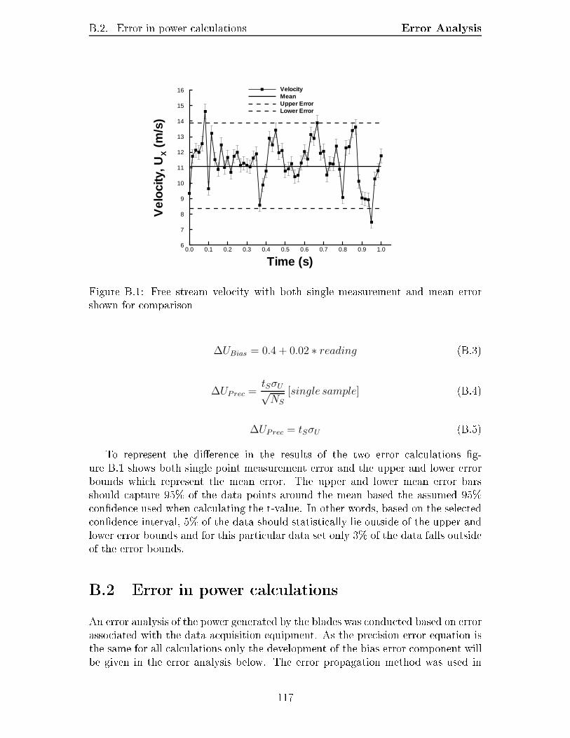
B.2. Error in power calculations Error Analysis

Time (s)

Vel

ocity

,UX

(m/s

)

0.0 0.1 0.2 0.3 0.4 0.5 0.6 0.7 0.8 0.9 1.06

7

8

9

10

11

12

13

14

15

16 VelocityMeanUpper ErrorLower Error

Figure B.1: Free stream velocity with both single measurement and mean errorshown for comparison∆UBias = 0.4 + 0.02 ∗ reading (B.3)∆UPrec =

tSσU√NS

[single sample] (B.4)∆UPrec = tSσU (B.5)To represent the dierence in the results of the two error calculations g-ure B.1 shows both single point measurement error and the upper and lower errorbounds which represent the mean error. The upper and lower mean error barsshould capture 95% of the data points around the mean based the assumed 95%condence used when calculating the t-value. In other words, based on the selectedcondence interval, 5% of the data should statistically lie outside of the upper andlower error bounds and for this particular data set only 3% of the data falls outsideof the error bounds.B.2 Error in power calculationsAn error analysis of the power generated by the blades was conducted based on errorassociated with the data acquisition equipment. As the precision error equation isthe same for all calculations only the development of the bias error component willbe given in the error analysis below. The error propagation method was used in117

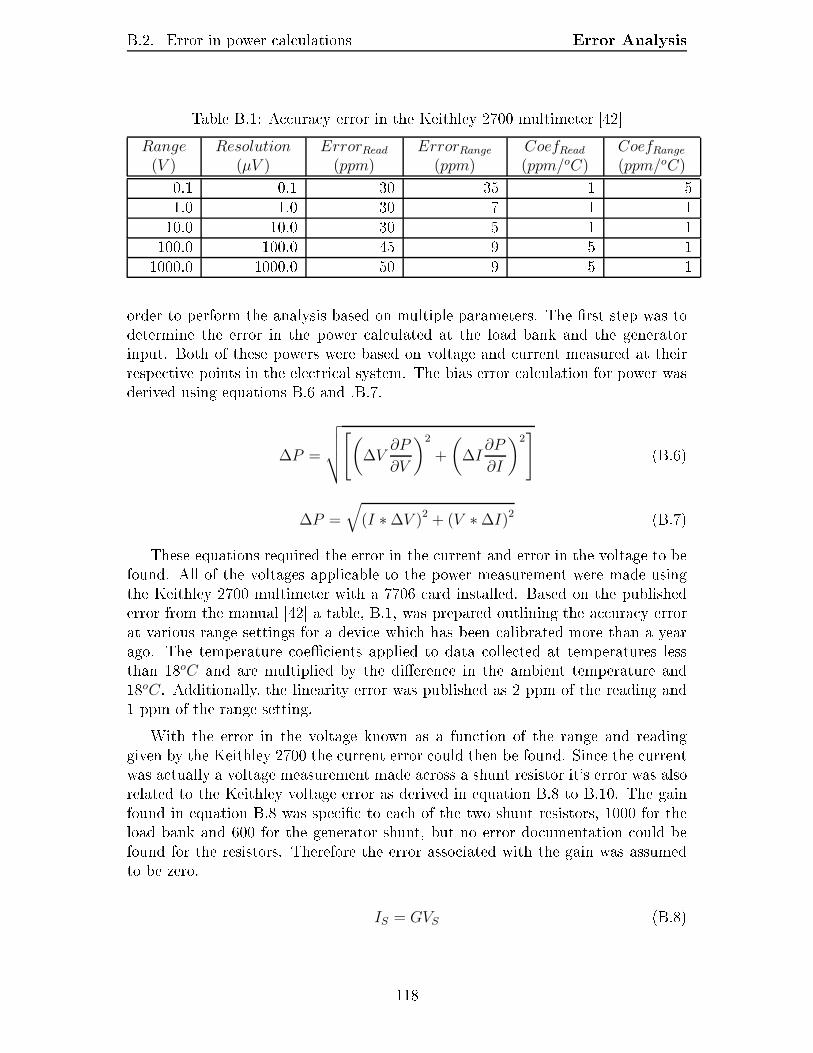
B.2. Error in power calculations Error AnalysisTable B.1: Accuracy error in the Keithley 2700 multimeter [42]Range(V )

Resolution(µV )

ErrorRead

(ppm)ErrorRange

(ppm)CoefRead

(ppm/oC)CoefRange

(ppm/oC)0.1 0.1 30 35 1 51.0 1.0 30 7 1 110.0 10.0 30 5 1 1100.0 100.0 45 9 5 11000.0 1000.0 50 9 5 1order to perform the analysis based on multiple parameters. The rst step was todetermine the error in the power calculated at the load bank and the generatorinput. Both of these powers were based on voltage and current measured at theirrespective points in the electrical system. The bias error calculation for power wasderived using equations B.6 and .B.7.∆P =

√

√

√

√

[

(

∆V∂P

∂V

)2

+

(

∆I∂P

∂I

)2] (B.6)

∆P =

√

(I ∗ ∆V )2 + (V ∗ ∆I)2 (B.7)These equations required the error in the current and error in the voltage to befound. All of the voltages applicable to the power measurement were made usingthe Keithley 2700 multimeter with a 7706 card installed. Based on the publishederror from the manual [42] a table, B.1, was prepared outlining the accuracy errorat various range settings for a device which has been calibrated more than a yearago. The temperature coecients applied to data collected at temperatures lessthan 18oC and are multiplied by the dierence in the ambient temperature and18oC. Additionally, the linearity error was published as 2 ppm of the reading and1 ppm of the range setting.With the error in the voltage known as a function of the range and readinggiven by the Keithley 2700 the current error could then be found. Since the currentwas actually a voltage measurement made across a shunt resistor it's error was alsorelated to the Keithley voltage error as derived in equation B.8 to B.10. The gainfound in equation B.8 was specic to each of the two shunt resistors, 1000 for theload bank and 600 for the generator shunt, but no error documentation could befound for the resistors. Therefore the error associated with the gain was assumedto be zero.IS = GVS (B.8)118

B.3. Error in coecient of power calculations Error Analysis∆I =

√

(

∆GδI

δG

)2

+

(

∆VδI

δV

)2 (B.9)∆I = G∆V (B.10)The error in the power generation value could then be found as the sum ofthe errors from the load bank power and the generator input power as these twovalues were subtracted when rst nding the generation power. The drivetrainpower loss was found to be a function of the rotational speed, as given by equa-tion B.11 and B.12, and therefore the drivetrain error was based on error in rota-tional speed and found using equations B.11 and B.12. The error in the rotationalspeed measurements, required to determine the power loss error, was solely dueto the clock accuracy in the digital counter which was specied as 50 ppm of thereading.[43]

∆PDrive =

√

(

∆ΩδPDrive

δΩ

)2 (B.11)∆PDrive =

√

(∆Ω (−0.0054 ∗ Ω − 2.1165))2 (B.12)The estimated power at the blades was derived from dierence between thepower measured during testing and the drivetrain power loss estimate so the overallerror was found by summing the two error values, found in equation B.13.∆PBlade = ∆PGEN + ∆PDrive (B.13)Since the bias error was specic to each reading there was no set value to applyto all data points. But the error range for the blade power was typically on theorder of 1 to 2% after outlier points are removed which can skew the precision errorestimate.B.3 Error in coecient of power calculationsThe error propagation calculations for the coecient of power were derived fromequation 2.11 and are outlined in equations B.14 to B.15.

∆CP =

√

(

∆PBlade

δCP

δPBlade

)2

+

(

∆ρδCP

δρ

)2

+

(

∆UδCP

δU

)2

+

(

∆RT

δCP

δRT

)2(B.14)119

B.3. Error in coecient of power calculations Error Analysis∆CP =

2PBlade

πρU3R2

√

(

∆PBlade

PBlade

)2

+

(

∆ρ

ρ

)2

+

(

3∆U

U

)2

+

(

2∆R

R

)2 (B.15)The error in the blade power estimates is detailed above. While the error in thedensity calculation was determined using the equations B.16 through to B.17. Thepressure data used in the density calculations were from the University of Water-loo weather station based on the average of the data collected during the testinghours.[48] This pressure data has a stated error of +/- 20 Pa. The temperaturedata was collected by a thermocouple found in the CSAT3 anemometer and wascollected at the same frequency as the velocity data and has an error of +/- 0.4 oC.ρ =

P

RT(B.16)

∆ρ =

√

(

∆P1

RT

)2

+

(

∆TP

RT 2

)2 (B.17)The error in the velocity data collected using the CSAT3 sonic anemometer wasgiven in the device specications as +/- 0.04 m/s with a gain error of +/- 2% ofthe reading. The blade radius error was taken as half the smallest increment onthe tape measure used and was therefore +/- 0.5 mm.The resulting error in the coecient of power was specic to each data point butwas representative error values were typically around 7% of the calculated value.

120

Appendix CInstallation and Decommissioning ofthe Wind TurbineThe installation of the nacelle and tower was a multi-stage process with decommis-sioning being completed in the reverse order. The tower was initially assembled ina horizontal position with both sets of axial legs and one set of lateral legs boltedonto the base of the tower poles. The tower was then raised so that the towerpoles were in a vertical position and the nal set of lateral legs were bolted to thestructure. The tower base was then moved to the nal position in the wind facilityand bolted to the ground using concrete mounts. The axial thrust bracing was theninstalled to stien the structure. Torque bracing must be installed after the nacelleis mounted to the towers as the guy wires interfered with the material lift used toraise the nacelle.In order to install the nacelle onto the tower a mechanical material lift wasutilized as the nal height of the mounting point was approximately 3 m fromground level and the nacelle weighed approximately 230 kg. After the lift wascompleted the nacelle was xed to the tower by eight bolts on matching mountingplates. The manually operated material lift raising the nacelle to the mountingpoint is shown in gures C.1 and C.2.The three turbine blades were then mounted to the low speed shaft on thenacelle. All three blades were mounted to the adapter plate, which interfaces withthe plate welded to the low speed shaft, while on level ground. Then using thematerial lift all three blades are lifted into position on the low speed shaft. Thismethod was used as it was dicult to achieve the correct blade alignment whenmounting the blades individually while at the 3.5 m shaft height. Overall theinstallation process, when completed eciently and with an adequate number ofpeople, can be completed in approximately two to three hours.

121

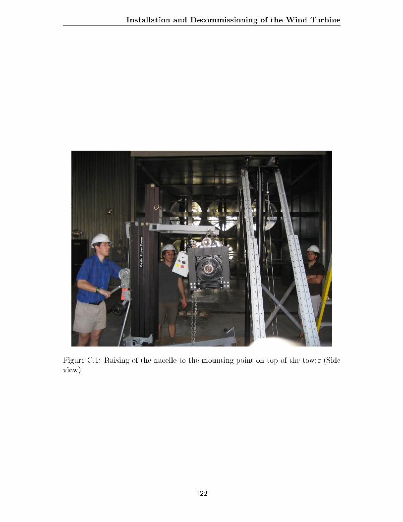
Installation and Decommissioning of the Wind Turbine

Figure C.1: Raising of the nacelle to the mounting point on top of the tower (Sideview)

122

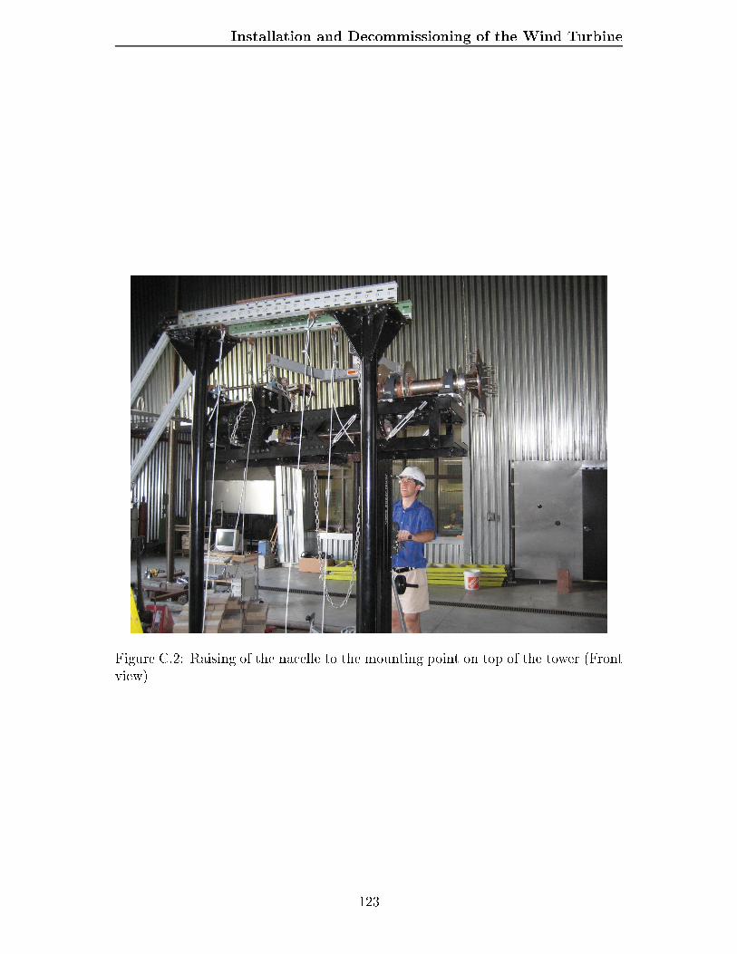
Installation and Decommissioning of the Wind Turbine

Figure C.2: Raising of the nacelle to the mounting point on top of the tower (Frontview)

123

Appendix DTurbine Blade FabricationThe turbine blade fabrication process was completed using the technique outlinedin the following sections.D.1 Mould and Material PreparationThe mould, shown in gure D.1, was a two piece structure with three locating pinsfor joining the two sides. The two mould halves were not identical as one was muchdeeper at the root section and will be referred to as the bottom half with theshallow side being the top half. Before each blade was manufactured the twosided mould was prepared for the moulding process by ensuring the mould was freeof debris and applying a high temperature mould release wax to the inner surfaces.Based on the lamination schedule, produced by Composotech [30], various typesof breglass were cut and prepared for all three blades. Each blade required sevendierent layers of breglass with three dierent materials used. For each blademould half the following material was cut: a skin layer, three structural layers,three spar support layers and one spar cover layer. An overview of the blade andthe positions used in the placement of the layers is shown in gure D.2.The skin layer, while providing some structure, is primarily to form the aerody-namic shape of the blade. It was comprised of 300 g/m2 chopped strand mat (csm)breglass 30.5 cm wide and 226 cm long. The three structural layers were madeusing a 600 g/m2 triax material which has strands in the chordwise direction and at+/- 45 degrees to the chord. This layer provides shear and torsional strength to theblades. All three structural layers of triax were 20.3 cm wide prior to trimming andhad varying lengths which went to positions one, three and ve, from gure D.2.The spar support layers are made of a UD (uni-directional) strand material withbres running span-wise along the blade. These layers provide strength against thebending moment from thrust loading. The three layers of UD were cut to be 6.4cm wide and went to positions two, four and six. Finally the spar cover layer wasmade from triax 20.3 cm wide prior to trimming and went to position one.124

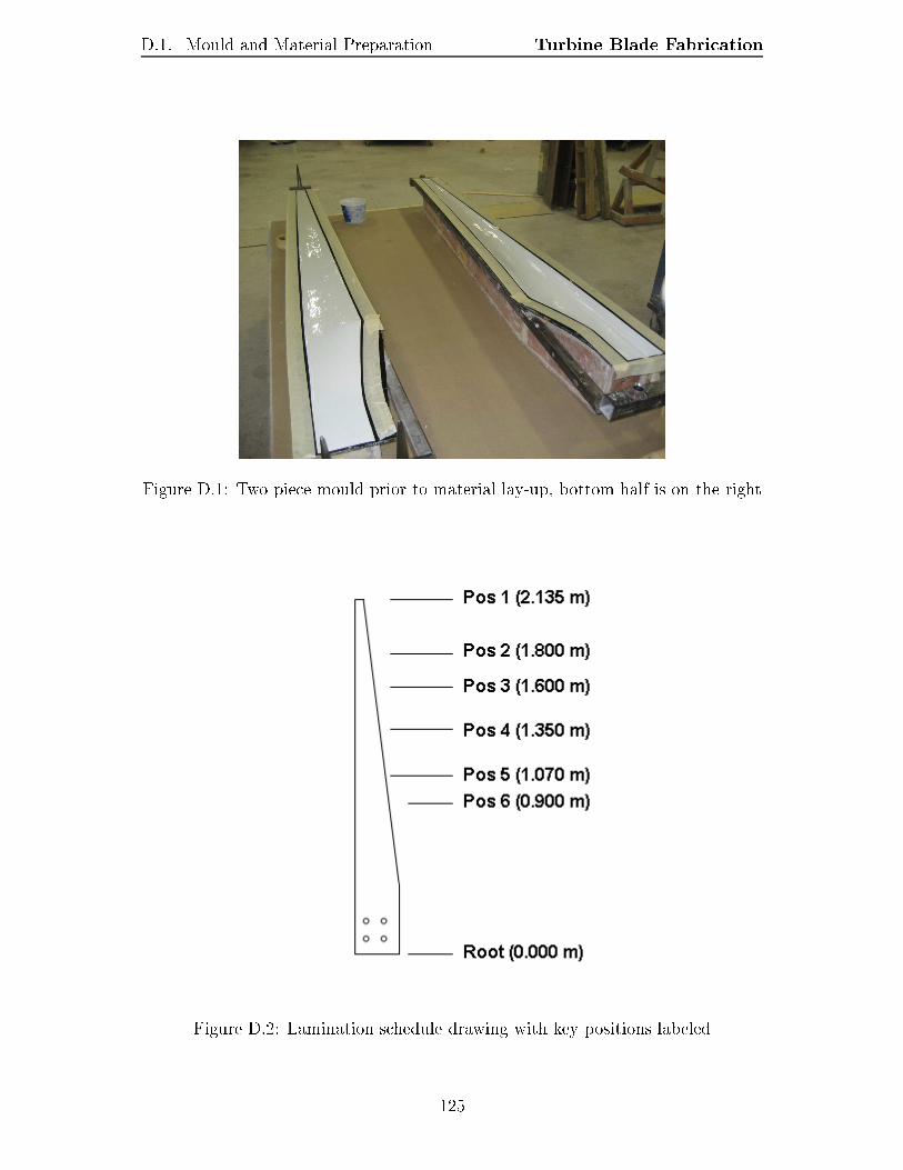
D.1. Mould and Material Preparation Turbine Blade Fabrication

Figure D.1: Two piece mould prior to material lay-up, bottom half is on the right

Figure D.2: Lamination schedule drawing with key positions labeled125

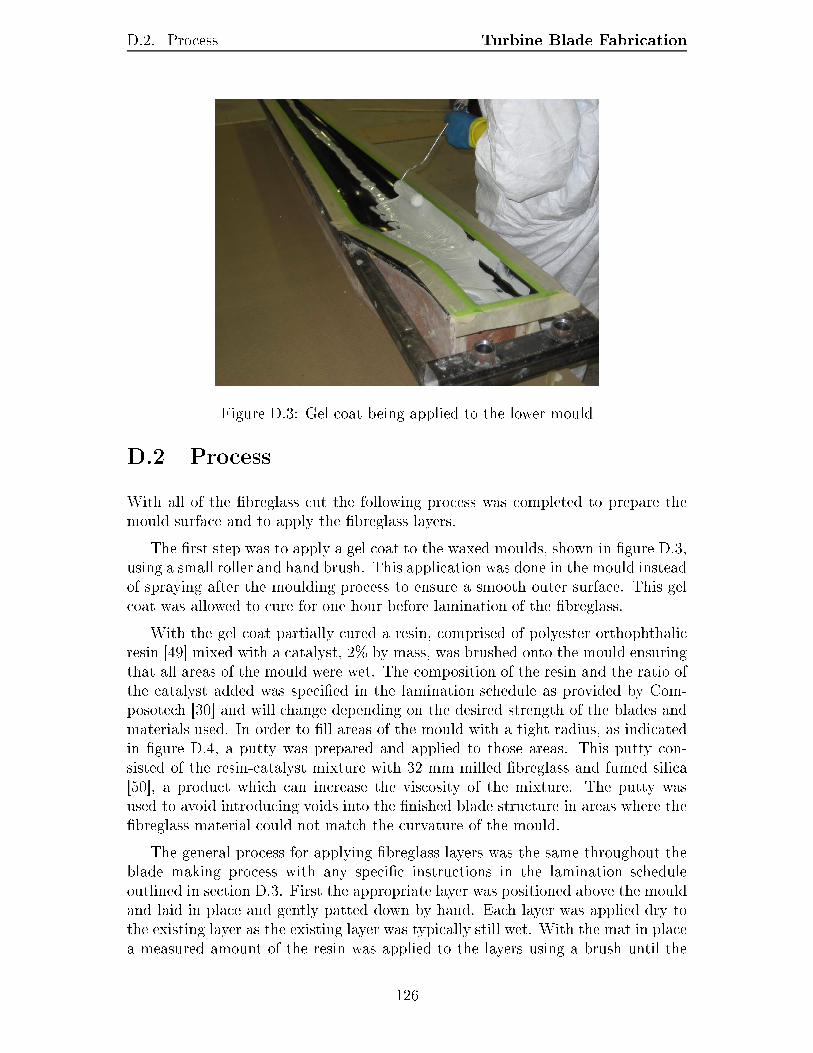
D.2. Process Turbine Blade Fabrication

Figure D.3: Gel coat being applied to the lower mouldD.2 ProcessWith all of the breglass cut the following process was completed to prepare themould surface and to apply the breglass layers.The rst step was to apply a gel coat to the waxed moulds, shown in gure D.3,using a small roller and hand brush. This application was done in the mould insteadof spraying after the moulding process to ensure a smooth outer surface. This gelcoat was allowed to cure for one hour before lamination of the breglass.With the gel coat partially cured a resin, comprised of polyester orthophthalicresin [49] mixed with a catalyst, 2% by mass, was brushed onto the mould ensuringthat all areas of the mould were wet. The composition of the resin and the ratio ofthe catalyst added was specied in the lamination schedule as provided by Com-posotech [30] and will change depending on the desired strength of the blades andmaterials used. In order to ll areas of the mould with a tight radius, as indicatedin gure D.4, a putty was prepared and applied to those areas. This putty con-sisted of the resin-catalyst mixture with 32 mm milled breglass and fumed silica[50], a product which can increase the viscosity of the mixture. The putty wasused to avoid introducing voids into the nished blade structure in areas where thebreglass material could not match the curvature of the mould.The general process for applying breglass layers was the same throughout theblade making process with any specic instructions in the lamination scheduleoutlined in section D.3. First the appropriate layer was positioned above the mouldand laid in place and gently patted down by hand. Each layer was applied dry tothe existing layer as the existing layer was typically still wet. With the mat in placea measured amount of the resin was applied to the layers using a brush until the126

D.3. Fibreglass Lamination Schedule Turbine Blade Fabrication

Figure D.4: Areas of the mould which required putty to ll small radius areasmat was saturated. The level of saturation in the breglass will aect the colourit has and an experienced worker can apply the correct amount of resin based onthis colour. Visible bubbles in the breglass were then removed using a metal rollerwhich allows the resin to be evenly distributed along the blade. If required a smallbrush with resin on it or a exible putty blade can be used to remove any remainingbubbles. Some bubbles under the breglass layers at the edges of the mould werenot required to be removed as they were outside of the nished blade area as shownin gure D.5. Care was taken throughout this process to monitor how much resinwas being used to avoid a resin rich or bre rich blade. If too much resin is usedthe blade can become brittle whereas too little resin could make the blade weakand in the extreme will result in delamination. The desired breglass to resin ratio,by mass, for this blade was 50/50 by Composotech design [30].D.3 Fibreglass Lamination ScheduleThe lamination schedule prepared by Compostech is outlined below with details ofeach layer's application and the techniques used during the process. A cutaway ofthe nal structure can be found in gure D.6, with the solid line representing theskin layer, the dashes representing triax, dots with a line representing UD and thehatched area representing the foam core.127

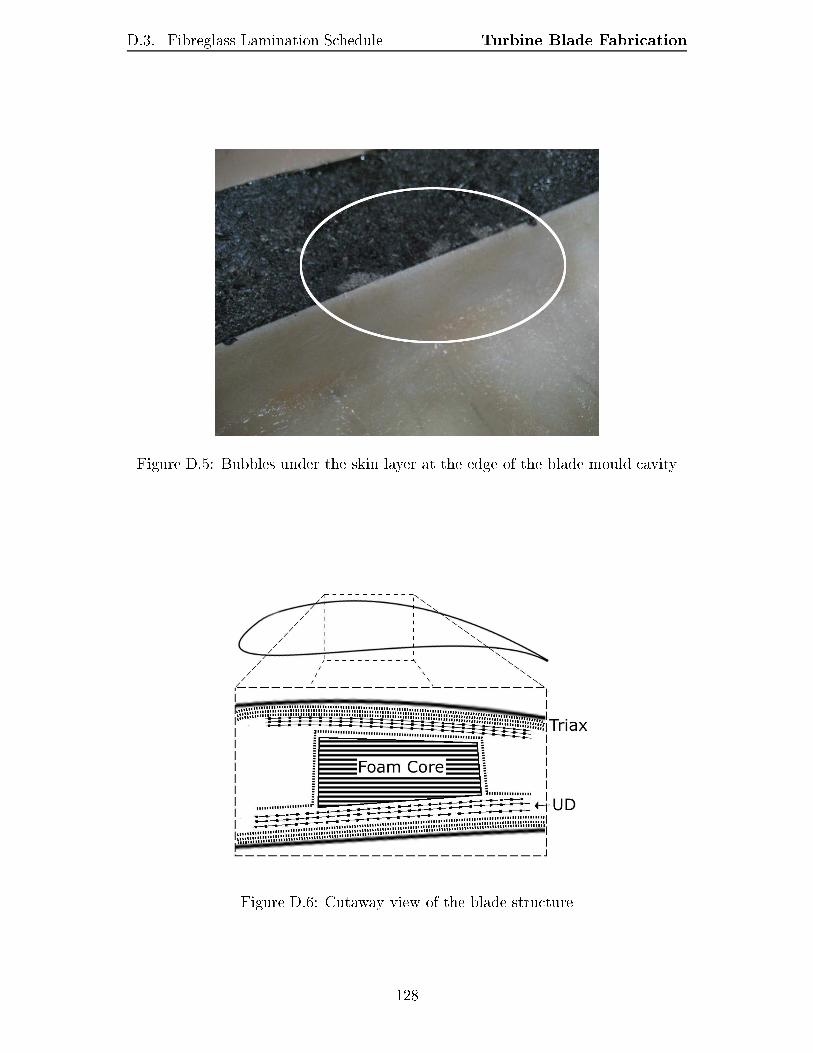
D.3. Fibreglass Lamination Schedule Turbine Blade Fabrication

Figure D.5: Bubbles under the skin layer at the edge of the blade mould cavity

Figure D.6: Cutaway view of the blade structure128

D.4. Skin Layer Turbine Blade Fabrication

Figure D.7: Skin layer cuts made to avoid wrinkles in bottom half of the mouldD.4 Skin LayerThe 300 csm skin layer was the rst layer of breglass applied to the mould and assuch the mould was coating in resin prior to it's application. Excess material was cutfrom around the edge of the mould plates which left an area on each side of the bladecavity covered. Cuts are made to the skin layer on the bottom half perpendicularto the mould edge to avoid wrinkles in the surface, shown in gure D.7. The skinlayer was allowed to cure for one hour prior to further application of breglass.D.4.1 Second Lamination - triaxThe second layer of breglass was a triax layer applied directly to the skin layerusing the longest of the triax mats. It was applied with one of the edges of themat aligned with the leading edge of the blade cavity in the mould. The trailingedge of the mat was then trimmed to be 1 cm from the mould edge at the tip, asshown in gure D.8, and approximately 2 cm at the root. This is done to achievea sharp trailing edge at the end of the process. Alternatively, the trailing edge canbe sanded down to achieve the desired thickness.D.4.2 Third and Fourth Lamination - triaxBoth the third and fourth laminations were applied while the previous layer wasstill wet with each layer becoming progressively shorter with excess resin removedor redistributed. The moulds with the breglass layers to this point can be seen129

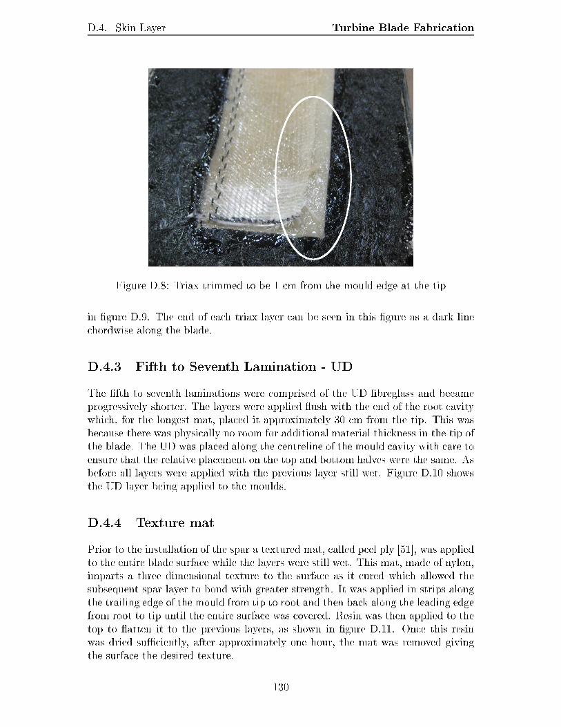
D.4. Skin Layer Turbine Blade Fabrication

Figure D.8: Triax trimmed to be 1 cm from the mould edge at the tipin gure D.9. The end of each triax layer can be seen in this gure as a dark linechordwise along the blade.D.4.3 Fifth to Seventh Lamination - UDThe fth to seventh laminations were comprised of the UD breglass and becameprogressively shorter. The layers were applied ush with the end of the root cavitywhich, for the longest mat, placed it approximately 30 cm from the tip. This wasbecause there was physically no room for additional material thickness in the tip ofthe blade. The UD was placed along the centreline of the mould cavity with care toensure that the relative placement on the top and bottom halves were the same. Asbefore all layers were applied with the previous layer still wet. Figure D.10 showsthe UD layer being applied to the moulds.D.4.4 Texture matPrior to the installation of the spar a textured mat, called peel ply [51], was appliedto the entire blade surface while the layers were still wet. This mat, made of nylon,imparts a three dimensional texture to the surface as it cured which allowed thesubsequent spar layer to bond with greater strength. It was applied in strips alongthe trailing edge of the mould from tip to root and then back along the leading edgefrom root to tip until the entire surface was covered. Resin was then applied to thetop to atten it to the previous layers, as shown in gure D.11. Once this resinwas dried suciently, after approximately one hour, the mat was removed givingthe surface the desired texture. 130

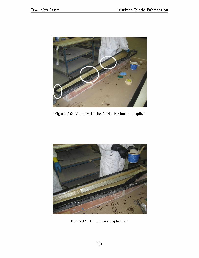
D.4. Skin Layer Turbine Blade Fabrication

Figure D.9: Mould with the fourth lamination applied

Figure D.10: UD layer application131

D.5. Spar Turbine Blade Fabrication

Figure D.11: Textured mat applicationD.5 SparThe nal component of the blades to be made was the spar. This spar provided acore to the blade and helped to connect the top and the bottom halves. Structurallythe spar was similar to the web of an I-beam with the nal three layers of UD oneach blade acting as the anges. The spar consisted of a foam core with triax600 g/m2 breglass laid on top. The rst step to making the core section was tomeasure the depth of the mould halves at regular intervals from root to tip. Thedepths were added together to determine the required thickness of foam to contactthe two halves when they were mated with 4 mm subtracted from this value tocompensate for the thickness of the nal triax layer applied to the foam core. Eachblades core was hand cut based on depth measurements of the mould halves whichresulted in a wedge shaped foam block. The spar block was then placed in thebottom of the mould and the nal triax layer was wrapped over it with a similartechnique as previous layers. Excess triax material was trimmed from the sides ofthe spar while maintaining a minimum of 25 mm on each side of the foam block.D.6 Mating MouldsThe rst step of the mating process is to determine the gaps in between the mouldhalves. The spar was rst positioned in the bottom mould dry. With the spar inplace plasticine balls were placed along the top of the spar and around the perimeterof the trailing and leading edges. The two mould halves were then compressedtogether and then released. The thickness of the plasticine after being compressedwill then represent the gap between the two moulds. Ideally this gap is 2 mm which132

D.6. Mating Moulds Turbine Blade Fabricationallows for sucient putty to remain in the joint to bond the halves.The perimeter of the mould, spar and spar contact areas on the top and bottomof the mould were then coated in resin to prime the surfaces. Putty was appliedalong the outside of the blade cavity and along the spar contact areas. The sparwas then positioned in the bottom mould half and the two halves were joined andcompressed. They were held together for approximately twelve hours and thenseparated. At this point any excess breglass, resin or irregularities were removedand repaired.

133

Appendix EPIV Smoke Injection MethodsIn order to aid future PIV work which may be completed using this facility an at-tempt to catalogue some of the failed smoke injection methods for PIV are outlinedin this section.A failed attempt is depicted in gure E.1. The failed method shown placed thesmoke generator in the ow straightening section of the tunnel. This particularmethod was unsuccessful because the smoke generator was too far upstream fromthe turbine which resulted the smoke stream becoming too diuse giving a lowseeding particle density. In gure E.1 the smoke is shown to cover at least half ofthe blade at the rotor plane.The second method shown in gure E.2 placed the smoke generator approxi-mately 2 m upstream of the rotor plane with the smoke traveling through a 1 cmplastic tube into a straightening manifold. This method also resulting in the smokebeing too diuse while also having an excessive amount of condensate buildup whichblocked the ow of smoke within the tube.

134

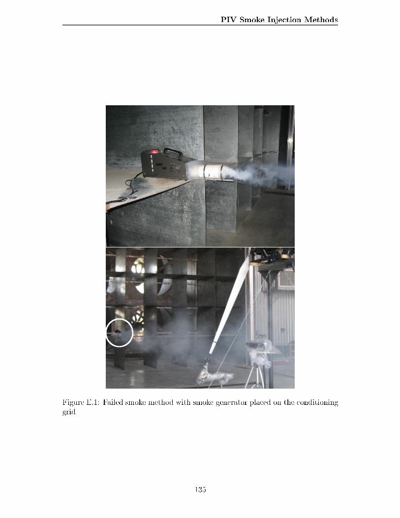
PIV Smoke Injection Methods

Figure E.1: Failed smoke method with smoke generator placed on the conditioninggrid135

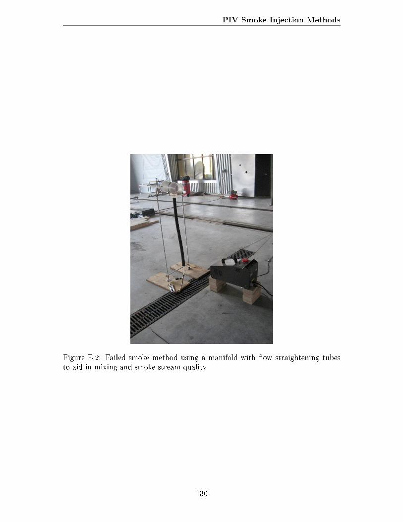
PIV Smoke Injection Methods

Figure E.2: Failed smoke method using a manifold with ow straightening tubesto aid in mixing and smoke stream quality

136

Appendix FPost Processing CodeThe post processing code used for the PIV analysis was comprised of two maincomponents: image shift determination, PIV data shift and shifted image output.F.1 Image Shift DeterminationThe following code is used to determine the number of pixels that each image wasshifted from a master image. These x and y shift values were then used to shift thePIV results calculated from the Flow Manager software [40].function output=s h i f t ( s ta r t ,num, f i l e n )shi f t_data=zeros (1 ) ;j=s t a r t ; %f i r s t imageth re s =100; %out l i e r thresholdimA='master_A . t i f ' ;for i =1:numimB0=' e : \ Test 1 export \ ' ;i f j <10imB1=' second_1_ .1 qqao5n5 .00000 ' ;e l s e i f j >=10 & j <100imB1=' second_1_ .1 qqao5n5 .0000 ' ;e l s e i f j >=100 & j <1000imB1=' second_1_ .1 qqao5n5 .000 ' ;else imB1=' second_1_ .1 qqao5n5 .00 ' ;endimB2=int2str ( j ) ;imB3=' . t i f ' ;imB=[imB0 , imB1 , imB2 , imB3 ] ;A=imread (imA) ;B=imread (imB) ;R = real ( i f f t 2 ( f f t2 (B) .∗ conj ( f f t2 (A) ) ) ) ;F=f f t s h i f t (R) ;[ maxval_F1 , I_F1 ] = max(F) ;[ maxval_F2 , I_F2 ] = max(maxval_F1 ) ;Xpos=I_F2 ;Ypos=I_F1(1 , I_F2) ;%Shi f t ing p lo t axes to correspond to corre lat ion p lo t[X,Y]=meshgrid (−504:503 ,−509:508) ;x s h i f t=X(1 ,Xpos ) ;y s h i f t=Y(Ypos , 1 ) ∗−1;x in t=round( x s h i f t /16) ;y in t=round( y s h i f t /16) ; 137

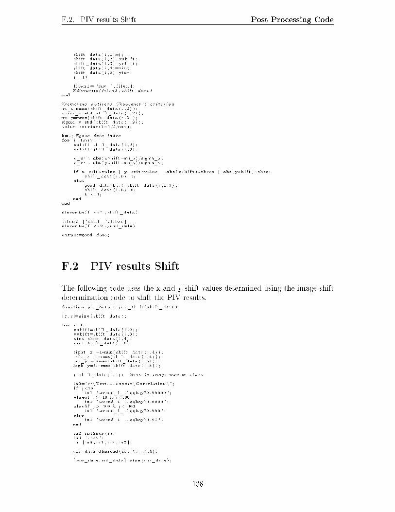
F.2. PIV results Shift Post Processing Codeshi f t_data ( i , 1 )=j ;shi f t_data ( i , 2 )=x s h i f t ;sh i f t_data ( i , 3 )=y s h i f t ;sh i f t_data ( i , 4 )=x int ;sh i f t_data ( i , 5 )=y int ;j=j+1f i l e n 1 =[ 'raw_ ' , f i l e n ] ;%dlmwrite ( f i l en1 , shift_data )end%removing ou t l i er s Chauvenet ' s cr i t er ionmu_x=mean( shi f t_data ( : , 2 ) ) ;sigma_x=std ( shi f t_data ( : , 2 ) ) ;mu_y=mean( shi f t_data ( : , 3 ) ) ;sigma_y=std ( shi f t_data ( : , 2 ) ) ;va lue=norminv (1−1/4/num) ;k=1; %good data indexfor i =1:numx s h i f t=shi f t_data ( i , 2 ) ;y s h i f t=shi f t_data ( i , 3 ) ;x_cr it=abs ( x s h i f t−mu_x)/sigma_x ;y_cr it=abs ( y s h i f t−mu_y)/sigma_y ;i f x_crit>value | y_crit>value | abs ( x s h i f t )>thre s | abs ( y s h i f t )>thre sshi f t_data ( i , 6 ) =1;else good_data (k , : )=shi f t_data ( i , 1 : 5 ) ;sh i f t_data ( i , 6 ) =0;k=k+1;endenddlmwrite ( f i l e n 1 , shi f t_data )f i l e n 2 =[ ' sh i f t_ ' , f i l e n ] ;dlmwrite ( f i l e n 2 , good_data )output=good_data ;F.2 PIV results ShiftThe following code uses the x and y shift values determined using the image shiftdetermination code to shift the PIV results.function piv_output=piv_sh i f t ( shi f t_data )[ r , c ]= s ize ( shi f t_data ) ;for i =1: rx s h i f t=shi f t_data ( i , 2 ) ;y s h i f t=shi f t_data ( i , 3 ) ;x in t=shi f t_data ( i , 4 ) ;y in t=shi f t_data ( i , 5 ) ;right_x=−1∗min( shi f t_data ( : , 4 ) ) ;l e f t_x=61−max( shi f t_data ( : , 4 ) ) ;low_y=−1∗min( shi f t_data ( : , 5 ) ) ;high_y=61−max( shi f t_data ( : , 5 ) ) ;j=shi f t_data ( i , 1 ) ; %set to image number s t a r tin0=' e : \ Test 1 export \ Cor r e l a t i on \ ' ;i f j <10in1=' second_1_ .1 qqkqy79 .00000 ' ;e l s e i f j >=10 & j <100in1=' second_1_ .1 qqkqy79 .0000 ' ;e l s e i f j >=100 & j <1000in1=' second_1_ .1 qqkqy79 .000 ' ;else in1=' second_1_ .1 qqkqy79 .00 ' ;endin2=int2str ( j ) ;in3=' . txt ' ;in=[ in0 , in1 , in2 , in3 ] ;cor_data=dlmread ( in , ' \ t ' , 5 , 0 ) ;[ row_data , col_data ]= s ize ( cor_data ) ; 138

F.3. Image Shifting Post Processing Codek=1;for m=1:row_datax_num=cor_data (m, 1 )−x int ;y_num=cor_data (m, 2 )−y int ;i f x_num>=right_x & x_num<=le f t_x & y_num>=low_y & y_num<=high_ynew_cor_data (k , 1 )=x_num;new_cor_data (k , 2 )=y_num;new_cor_data (k , 3 )=cor_data (m,1 0 ) ;new_cor_data (k , 4 )=cor_data (m,1 1 ) ;new_cor_data (k , 5 )=cor_data (m, 3 )−x s h i f t ;new_cor_data (k , 6 )=cor_data (m, 4 )−y s h i f t ;new_cor_data (k , 7 )=cor_data (m,1 2 ) ;k=k+1;endendout1=' co r_sh i f t \second_1_ ' ;out=[out1 , in2 , in3 ] ;%dlmwrite (out ,new_cor_data , '\ t ' ) ;piv_output ( : , : , i )=new_cor_data ;j=j +1;iendF.3 Image ShiftingFor program verication and for the presentation of results a program was alsowritten to crop and shift the images based on the x and y shift results.shi f t_data=dlmread ( ' shift_0_9 . txt ' ) ;[ r , c ]= s ize ( shi f t_data ) ;for i =1: rj=shi f t_data ( i , 1 ) ;imB0=' t e s t 1 \ ' ;i f j <10imB1=' second_1_ .1 qqao5n5 .00000 ' ;e l s e i f j >=10 & j <100imB1=' second_1_ .1 qqao5n5 .0000 ' ;e l s e i f j >=100 & j <1000imB1=' second_1_ .1 qqao5n5 .000 ' ;else imB1=' second_1_ .1 qqao5n5 .00 ' ;endimB2=int2str ( j ) ;imB3=' . t i f ' ;imB=[imB0 , imB1 , imB2 , imB3 ] ;A=imread (imB) ;%figure ; imshow(A) ;x s h i f t=shi f t_data ( i , 2 ) ;y s h i f t=shi f t_data ( i , 3 ) ;for k=1:1018for m=1:1008i f (k−y s h i f t )>0 & (m+x s h i f t )>0 & (k−y s h i f t )<=1018 & (m+x s h i f t )<=1008new_A(k ,m)=A(k−y sh i f t ,m+x s h i f t ) ;elsenew_A(k ,m)=0;endendend%figure ; imshow(new_A) ;f i l e n =[ ' imsh i f t \ shi f ted_ ' , int2str ( j ) , ' . t i f ' ]imwrite (new_A, f i l e n )end139