Winner of the 2018 PROSE Award in Engineering & Technology

Fully Updated Hydrology Principles, Methods, and Applications

This industry-standard resource has been completely revised for the first time since Ven Te Chow'sclassic edition was published over 50 years ago. Compiled by a colleague of the late Dr. Chow andfeaturing chapter contributions from a “who’s who” of international hydrology experts, Handbookof Applied Hydrology, Second Edition, covers scientific and engineering fundamentals and presents all-new methods, processes, and technologies. Complete details are provided for the fullrange of ecosystems and models. Advanced chapters look to the future of hydrology, includingclimate change impacts, extraterrestrial water, social hydrology, and water security.

Publisher : McGraw-Hill Education; 2nd Edition (November 1, 2016)ISBN: 9780071835091

34-1

ABSTRACT

Adomian’s decomposition method (ADM) constitutes a useful alternative to model linear, and especially nonlinear, equations in surface, subsurface, and contaminant hydrology. ADM offers the advantages of both analytical and numerical procedures, while minimizing many of their disadvantages. It exhibits the simplicity, stability, and spatial and temporal continuity of ana-lytical solutions, in addition to the ability to handle irregularly shaped domains, and nonlinearity typical of numerical solutions. The most impor-tant feature in ADM is its simplicity; many problems that were considered tractable by complex numerical methods only, are now easily approached with ADM. This chapter presents a simple introduction to the features of ADM with some application examples to the modeling of various phenomena in hydrology. These include nonlinear kinematic and dynamic flood waves, infiltration under variable rainfall, nonlinear soil moisture propagation, groundwater flow in irregularly shaped aquifers, groundwater flow in hetero-geneous aquifers subject to pumping and recharge, stream-aquifer interac-tion, propagation of nonlinear hydraulic transients in aquifers, contaminant transport in soils and aquifers subject to nonlinear reactions, and stochastic analysis in hydrology without small perturbation restrictions.

34.1 INTRODUCTION: ADOMIAN’S DECOMPOSITIONS METHOD

The fundamental building blocks of hydrologic models are usually made of partial differential equations governing fundamental laws in a watershed, a soil, or an aquifer. Traditionally, these equations must be solved analytically or numerically. Classical analytical solutions (e.g., Fourier series and Laplace transform) are simple to program, are usually stable, and offer a spatially and temporally continuous description of hydrologic variables (e.g., Steward et al., 2009; Read, 2007; Read and Volker, 1993; Chapman and Dressler, 1984; Kirkham, 1957; and Philip, 1957). However, classical ana-lytical solutions require regular domain shapes (e.g., simple one-dimension-al or rectangular geometries), and cannot handle nonlinearities. On the other hand, numerical solutions (e.g., finite differences, finite elements, and finite volume) reduce the differential equations to a simpler system of alge-braic equations, can manage irregular domain shapes, and may deal with numerical approximations of nonlinearities. However, numerical solutions yield the state variables at discrete nodes only (i.e., they require a grid), are difficult to program (i.e., they require specialized computer software), and often have difficulties with instabilities and round-off errors. An alternative method, Adomian’s decomposition method (ADM; Adomian, 1994, 1991, 1986, 1983), offers the simplicity, stability, and spatial continuity of analyti-cal solutions, in addition to the ability to handle system nonlinearities and irregular geometries typical of numerical solutions. Many studies have reported new solutions to a wide class of equations (ordinary, partial, dif-ferential, integral, integrodifferential, linear, nonlinear, deterministic, or stochastic) in a variety of fields of mathematical physics, science, and engi-neering (see, e.g., Rach, Wazwaz, and Duan, 2013; Duan and Rach, 2011;

Rach, 2008; Wazwaz, 2000; Adomian, 1994, 1991). For nonlinear equations in particular, decomposition is one of the few systematic solution proce-dures available. Other analytical methods to solve nonlinear equations have been proposed, such as the homotopy perturbation method (e.g., He, 2006), and the variational iterations method (e.g., He, 1999), with few published applications in hydrology as yet.

ADM consists in deriving an infinite series that in many cases converge to an exact solution. The convergence of decomposition series has been rigor-ously established in the mathematical community (Gabet, 1994, 1993, 1992; Abbaoui and Cherruault, 1994; Cherruault, 1989; Cherruault et al., 1992), and in the hydrologic community (Serrano, 2003c, 1998). In many complex linear and nonlinear problems, an exact closed form solution is difficult to obtain. However, in these cases the usual fast convergence rate of decomposition series provides the modeler with a sufficiently accurate approximate solution. A convergent decomposition series made of the first few terms usually pro-vides an effective model in practical applications. With the concepts of partial decomposition and of double decomposition (Adomian, 1994, 1991), the process of obtaining an approximate solution was further simplified. Also, recent contributions suggest that the choice of the initial term greatly influ-ences the rate of convergence and the complexity in the calculation of indi-vidual terms, especially for nonlinear equations (Wazwaz and Gorguiz, 2004; Wazwaz, 2000). Thus, as long as the initial term in a decomposition series, usually the forcing function or the initial condition, is described in analytic form, a partial decomposition procedure may offer a simplified approximate solution to many modeling problems.

In hydrology, several fundamental works using decomposition have been published on groundwater flow (Moutsopoulos, 2007; Serrano, 1995; Serrano and Unny, 1987); analytical steady and transient groundwater modeling in irregularly shaped aquifers (Serrano, 2013, 2012; Patel and Serrano, 2011; Tiaiff and Serrano, 2014); fracture flow (Moutsopoulos, 2009); contaminant transport (Serrano, 1988; Adomian and Serrano, 1998; Serrano and Adomian, 1996); special problems involving non-Fickian and scale-dependent contami-nant transport (Serrano, 1997b, 1996, 1995b); hydraulics of wells in heteroge-neous aquifers (Serrano, 1997a); stream-aquifer interaction (Serrano and Workman, 2008, 1998; Serrano et al., 2007; Srivastava et al., 2006); modeling in heterogeneous aquifers (Srivastava and Serrano, 2007; Serrano, 1995a); nonlinear moving boundaries in unconfined aquifers (Serrano, 2003a); infil-tration in unsaturated and hysteretic soils (Serrano, 2004, 2003b, 2001, 1998, 1990a); catchment hydrology and nonlinear flood propagation (Serrano, 2006; Sarino and Serrano, 1990); nonlinear reactive contaminant transport (Serrano, 2003c); and sediment transport in alluvial streams (Tayfur and Singh, 2011). Several fundamental problems that were considered tractable with numerical methods only have been easily approached with decomposi-tion. Besides simplicity, an analytical solution offers a continuous spatio temporal distribution in heads, gradients, velocities and fluxes, thus reducing instability. Combination of analytical decomposition with numerical methods offers an ideal modeling scenario that exhibits the advantages of both ana-lytical and numerical procedures (Serrano, 1992).

Chapter 34

Decomposition Methods

BY

SERGIO E. SERRANO

34_Singh_ch34_p34.1-34.6.indd 1 29/06/16 6:54 pm

34-2 DECOMPOSITION METHODS

where the integration “constants,” k3 and k4, are found from the y boundary conditions (34.2)

= + − +

−( ) ( ) ( )2 20 2

3 22

h f x f x f xl

R lT

yR y

Tyy

g y g (34.11)

The y-partial solution satisfies the differential Eq. (34.1) and the y bound-ary conditions in Eq. (34.2), but not necessarily those in the x direction. We now have two partial solutions to Eq. (34.1): the x-partial solution (34.7), and the y-partial solution (34.11). Since both are solutions to h, a combination of the two partial solutions yields

=

+

( , )

( , ) ( , )20

0 0h x yh x y h x yx y (34.12)

where h0 is the first combined term. Higher-order terms are derived similarly. The ith order term in the x-partial solution, hxi, may be derived from Eq. (34.5) as:

= + −+ +

−−( ) ( )4 1 4 2

11h k y k y x Lxi i i x L hy i (34.13)

where hi – 1 is the previous combined term in the decomposition series, and k4i + 1 k4i + 2 are such that homogeneous x boundary conditions in Eq. (34.2) are satisfied. Similarly, the ith-order term in the y-partial solution, hyi, may be derived from Eq. (34.9)

= + −+ +

−−( ) ( )4 3 4 4

11k x k x y L L hi i y x ihyi (34.14)

where hi – 1 is the previous combined term in the decomposition series, and k4i + 3 and k4i + 4 are such that homogeneous y boundary conditions in Eq. (34.2) are satisfied. Similarly to Eq. (34.12), the ith combined term is given by

=

+

( , )

( , ) ( , )2

h x yh x y h x y

ixi yi

(34.15)

Lastly, approximate the final solution with N terms, h ≈ h0 + h1 + …+ hN , where each term in the series is a combination of two partial solutions, one in x and one in y. The aforementioned procedure may be extended to three-dimensional transient problems. In such case, each combined term in the decomposition series has four components, one in each spatial coordinate, and one in the temporal coordinate. Due the high rate of convergence of decomposition solutions, the hydrologist often finds that few terms in the above iteration might be reasonably accurate in many practical applications.

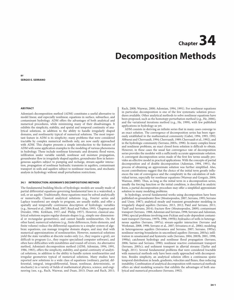
In this example, the first three terms at the center of the aquifer x = lx/2, y = ly/2 are h0 = 248.52 m, h1 = 5.46 m, and h2 = 2.13 m. It is easy to program the aforementioned solution in any standard mathematics software, such as Maple. Figure 34.1 shows the regional groundwater flow distribution. Patel and Serrano (2011) showed that the maximum relative error of a four-term decomposition solution with respect to the exact analytical solution of a similar problem is less than 2%. Serrano (2012) also showed similar results when comparing a transient regional groundwater flow with respect to its exact analytical solution. Consideration of pumping wells at known coordi-nates in the aquifer is an easy extension to the aforementioned description. Similarly, aquifer heterogeneity, nonlinearity in the differential equation, and irregular aquifer geometries can be incorporated into the analysis (Tiaif and Serrano, 2014, 2013; Patel and Serrano, 2011). For practical examples with detailed programs, see Serrano (2010).

34.3 PROPAGATION OF NONLINEAR KINEMATIC FLOOD WAVES IN RIVERS

This section illustrates the application of ADM series, double decomposition, and successive approximation to the solution of nonlinear hydrologic prob-lems. Consider the following nonlinear kinematic flood routing equation that combines the continuity and momentum equations, when the acceleration and the pressure terms in the latter are neglected:

αβ∂

∂+ ∂

∂

= = =β− , (0, ) ( ), ( ,0) (0)1Q

xQ Q

TQ Q t Q t Q x QL I I (34.16)

where Q(x, t) is the flow rate (m3/s); QL is the lateral flow into the channel per unit length (m3/s); x is the distance from a streamflow station with a known hydrograph; t is time (hour); a is a constant with dimensions (m2 – 3bsb); QI(t) is the inflow hydrograph at t = 0; and b is a dimensionless constant. Using the

34.2 REGIONAL FLOW IN AN UNCONFINED AQUIFER

This section illustrates the basis of ADM with a simple problem. For detailed introduction, practical examples in hydrology, and computer programs, see Serrano (2011, 2010). Consider the two-dimensional regional groundwater flow in an unconfined aquifer with Dupuit assumptions. The governing equa-tion is given by

hx

hy

x l y lx yRTg , 0 , 0

2

2

2

2∂∂

+ ∂∂

= − ≤ ≤ ≤ ≤ (34.1)

where h(x, y) is the hydraulic head; x and y are the planar coordinates with respect to an origin; the aquifer dimensions are lx = 860 m and ly = 2000 m, respectively; the aquifer transmissivity is T = 700 m2/month, and the mean recharge from rainfall is Rg = 10 mm/month. Equation (34.1) is subject to a mixed set of boundary conditions given by

h y f y h

xl y h x f x h x l f xx y(0, ) ( ), ( , ) 0, ( ,0) ( ), ( , ) ( )1 2 3= ∂

∂= = = (34.2)

where f1( y) = 241 – 0.001y, f2(x) = Cx2 + Ax + f1(0), f3(x) = Ex2 + Bx + f1(ly), C = –Rg /(2T), A = –2Clx, B = –2Elx, and E = –Rg /T. The functions f1, f2, and f3 have been derived from field measurements of the stage of the boundary rivers. Now define the operators Lx = ∂2/∂x2 and Ly = ∂2/∂y2. The inverse operators −1Lx and −1Ly are the corresponding twofold indefinite integrals with respect to x and y, respectively. Thus, Eq. (34.1) reduces to

L h L hx y

RTg+ = − (34.3)

Two partial decomposition expansions are possible: The x-partial solution and the y-partial solution. The x-partial solution, hx, results from operating with −1Lx on Eq. (34.3) and rearranging.

L hy xh L

RT

Lx xg

x1 1= − −− − (34.4)

Expanding hx in the right side as an infinite series hx = hx0 + hx1 + hx2 +… , Eq. (34.4) becomes

L h h hy x x xh L

RT

Lx xg

x ( )0 1 21 1= − − + + +− − (34.5)

The choice of hx0 often determines the level of difficulty in calculating subsequent terms and the rate of convergence (Adomian, 1994; Wazwaz, 2000). A simple choice is to set hx0 as equal to the first term in the right side of Eq. (34.5). Thus, the first approximation to the solutions is

h k y k y x

R xTx

gLRTxg ( ) ( )

20 1 2

21= − = + −− (34.6)

where the integration “constants,” k1 and k2, must be found from the x bound-ary conditions in Eq. (34.2). Hence, Eq. (34.6) becomes

h f y

R l xT

R xTx

g x g( )20 1

2

= + − (34.7)

Equation (34.7) satisfies the governing Eq. (34.1) and the x boundary con-ditions in Eq. (34.2), but not necessarily the ones in the y direction. Now, to obtain the y-partial solution to Eq. (34.3), hy, operate with Ly

−1 on Eq. (34.3) and rearrange

L hx yh L

RT

Ly yg

y1 1= − −− −

(34.8)

Expanding hy in the right side as an infinite series hy = hy0 + hy1 + hy2 +…, Eq. (34.8) becomes

L h h hx y y yh L

RT

Ly yg

y ( )0 1 21 1= − − + + +− − (34.9)

Taking hy0 as the first term in the right side of Eq. (34.9) one obtains the first approximation

h k x k x y

R yTy

gLRTyg ( ) ( )

20 3 4

21= − = + −− (34.10)

34_Singh_ch34_p34.1-34.6.indd 2 29/06/16 6:54 pm

PROPAGATION OF NONLINEAR KINEMATIC FLOOD WAVES IN RIVERS 34-3 

As stated, the convergence rate of ADM series is so high that only a few terms are needed to assure an accurate solution. Thus, if, for instance, Q02 is a reasonable approximation, then

≈ ≈ − + + + = −( [ ( ) ( ) ( )]) , ( , )0 0 0 1 0 2 0 0 02Q Q Q t x F f F f F f Q x f Q x t Q xI L L (34.21)

As an illustration, assume that a = 5/3, b = 3/5, QL = 0, and an inflow hydrograph given by

= + −

( )−( ) ( )0 max 0

max

1maxQ t q q q t

teI

tt (34.22)

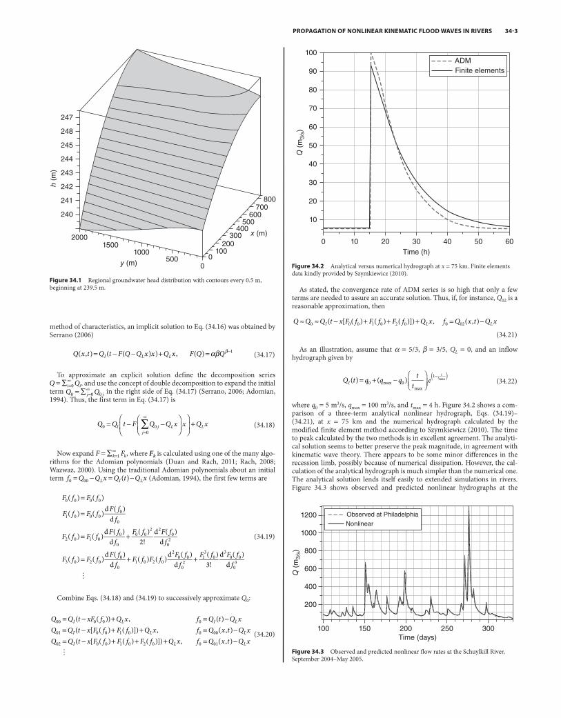
where q0 = 5 m3/s, qmax = 100 m3/s, and tmax = 4 h. Figure 34.2 shows a com-parison of a three-term analytical nonlinear hydrograph, Eqs. (34.19)–(34.21), at x = 75 km and the numerical hydrograph calculated by the modified finite element method according to Szymkiewicz (2010). The time to peak calculated by the two methods is in excellent agreement. The analyti-cal solution seems to better preserve the peak magnitude, in agreement with kinematic wave theory. There appears to be some minor differences in the recession limb, possibly because of numerical dissipation. However, the cal-culation of the analytical hydrograph is much simpler than the numerical one. The analytical solution lends itself easily to extended simulations in rivers. Figure 34.3 shows observed and predicted nonlinear hydrographs at the

method of characteristics, an implicit solution to Eq. (34.16) was obtained by Serrano (2006)

αβ= − − + = β−( , ) ( ( ) ) , ( ) 1Q x t Q t F Q Q x x Q x F Q QI L L (34.17)

To approximate an explicit solution define the decomposition series = ∑ =

∞0Q Qi i, and use the concept of double decomposition to expand the initial

term = ∑ =∞

0 0 0Q Qj j in the right side of Eq. (34.17) (Serrano, 2006; Adomian, 1994). Thus, the first term in Eq. (34.17) is

∑= − −

+

=

∞

0 00

Q Q t F Q Q x x Q xl j Lj

L (34.18)

Now expand = ∑ =∞

1F Fk k, where Fk is calculated using one of the many algo-rithms for the Adomian polynomials (Duan and Rach, 2011; Rach, 2008; Wazwaz, 2000). Using the traditional Adomian polynomials about an initial term = − = −( )0 00f Q Q x Q t Q xL I L (Adomian, 1994), the first few terms are

F f F f

F f F f F ff

F f F f F ff

F f F ff

F f F f F ff

F f F f F ff

F f F ff

( ) ( )

( ) ( )d ( )d

( ) ( )d ( )d

( )2!

d ( )d

( ) ( )d ( )d

( ) ( )d ( )d

( )3!

d ( )d

0 0 0 0

1 0 0 00

0

2 0 1 00

0

0 02 2

0

02

3 0 2 00

01 0 2 0

20 0

02

13

03

0 0

03

=

=

= +

= + +

(34.19)

Combine Eqs. (34.18) and (34.19) to successively approximate Q0:

= − + = −= − + + = −= − + + + = −

( ( )) , ( )( [ ( ) ( )]) , ( , )( [ ( ) ( ) ( )]) , ( , )

00 0 0 0

01 0 0 1 0 0 00

02 0 0 1 0 2 0 0 01

Q Q t xF f Q x f Q t Q xQ Q t x F f F f Q x f Q x t Q xQ Q t x F f F f F f Q x f Q x t Q x

I L I L

I L L

I L L

(34.20)

Figure 34.1 Regional groundwater head distribution with contours every 0.5 m, beginning at 239.5 m.

15002000

240

241

242

243

h (m

)

244

245

248

247

1000500y (m)

x (m)

00

100200

300400

500600

700800

Figure 34.2 Analytical versus numerical hydrograph at x = 75 km. Finite elements data kindly provided by Szymkiewicz (2010).

0

10

20

30

40

50

60

70

80

90

100

10 20 30Time (h)

Q (

m3/

s)

40 50 60

Finite elementsADM

Figure 34.3 Observed and predicted nonlinear flow rates at the Schuylkill River, September 2004–May 2005.

100

200

400

600

800

1000

1200

150 200Time (days)

250 300

Q (

m3/

s)

Observed at Philadelphia

Nonlinear

34_Singh_ch34_p34.1-34.6.indd 3 29/06/16 6:54 pm

34-4 DECOMPOSITION METHODS

This process may be continued: from Eq. (34.25), calculate D2, obtain an improved diffusivity D(q) ≈ D0 + D1 + D2, then similar to Eq. (34.28) derive θ ′3, then similar to Eq. (34.29) derive q3. Many studies report that ADM series converges fast and only a few terms are needed. Thus, q ≈ q3 may be a good approximation to the water content. Figure 34.4 shows profiles of the water content versus distance profiles at t = 1 h according to four sources: ADM, the classical numerical solution of Philip (1955), the numerical solu-tion of Parlange (1971), and laboratory observations (Serrano, 2004). The ADM solution appears to better predict the position of the wetting front, and the subsequent shape of the tail, than Philip’s (1955) or Parlange’s (1971) solutions. The decomposition solution is simpler; it provides a continuous spatio-temporal description, and it does not exhibit the stability and dis-cretization restrictions of numerical solutions. Extensions of ADM to physi-cally based vertical infiltration and distribution were derived by Serrano (2004). Simple physically based ADM models of infiltration in watersheds subject to variable rainfall have been proposed (Serrano, 2010, 2004). Explicit ADM solutions to the Green and Ampt equation were derived by Serrano (2003b, 2001).

34.5 SUMMARY AND CONCLUSIONS

The basic features of hydrologic modeling with ADM have been presented via three simple examples: regional groundwater flow in aquifers, the propagation of nonlinear kinematic flood waves in rivers, and nonlinear infiltration in unsaturated soils. ADM offers the advantages of both ana-lytical and numerical procedures, while minimizing many of their disad-vantages. It exhibits the simplicity, stability, and spatial and temporal continuity of analytical solutions, in addition to the ability to handle irregularly shaped domains, and nonlinearity typical of numerical solu-tions. ADM may be applied to a wide class of problems in hydrology, including, infiltration under variable rainfall, groundwater flow in irregu-larly shaped aquifers, groundwater flow in heterogeneous aquifers subject to pumping and recharge, stream-aquifer interaction, propagation of non-linear hydraulic transients in aquifers, contaminant transport in soils and aquifers subject to nonlinear reactions, and stochastic analysis in hydrology without small perturbation restrictions. Expanded references to such work, including practical computer programs, have been included. The most important feature in ADM is its simplicity; many problems that were con-sidered tractable by complex numerical methods only, are now easily approached with ADM. The method has proved invaluable to hydrologic analysis and preliminary design under scarce data. Future work should be devoted to the application of ADM to unresolved problems in nonlinear hydrology. As new algorithms for the Adomian polynomials continue to appear in the research literature, the possibilities to solved increasingly complex problems are promising.

Philadelphia station in the Schuylkill River (Southeast Pennsylvania), given an inflow hydrograph at the Norristown station (Serrano, 2006). The simula-tions included variable lateral flow that included groundwater flow and vari-able effective precipitation. The standard deviation of the absolute error between observed and predicted was only 13.21 m3/s.

34.4 NONLINEAR INFILTRATION IN UNSATURATED SOILS

This section presents a combination of ADM with a successive approximation (Serrano, 2004) that yields a simple approximate solution to a highly nonlin-ear equation, when traditional numerical solutions present numerous accuracy, complexity, and instability problems. Consider the horizontal infil-tration equation in a semi-infinite homogeneous soil with a constant bound-ary condition maintained on one end:

θ θ θ θ θ θ θ θ θ∂∂

− ∂∂

∂∂

= < < ∞ < = ∞ = =( ) 0, 0 , 0 , (0, ) , ( , ) , ( ,0)t x

Dx

x t t t xb i i

(34.23)

where q = soil volumetric water content; x = horizontal distance (m); t = time (h); qb = 0.458 is the water content at the left boundary; qi = 0.086 is the initial water content; θ = λθα

( ) e1D c is the soil-water diffusivity (m2/h); c1 = 1 m2/h; l = 500; and a = 11 (Serrano, 1998). Expanding the nonlinear diffusivity as the series θ = ∑ =

∞( ) 0D Di i , Eq. (34.23) becomes

∑θ θ∂

∂− ∂

∂

∂∂

==

∞

00t x

Dxi

i (34.24)

Similar to Eq. (34.19), the Adomian polynomials about the first term, q0, are given by (Adomian, 1994)

D D

D D

D D D

D D D D

b

( )d ( )

d

d ( )d 2!

d ( )d

d ( )d

d ( )d 3!

d ( )d

0

1 10

0

2 20

0

02 2

0

02

3 30

01 2

20

02

13 3

0

03

θ

θ θθ

θ θθ

θ θθ

θ θθ

θ θ θθ

θ θθ

=

=

= +

= + +

(34.25)

Now recursively calculate each Di, which is used to approximate the next qi. Calculations end when the water content distribution reaches a desired accuracy. From Eq. (34.25), use the left boundary condition, q ≈ qb, as an initial estimate of the water content. With the approximation D(q) ≈ D0 = D(q b), Eq. (34.24) reduces to the classical heat flow equation with constant coefficient whose solution is (Zauderer, 1983)

θ θ θ θ= + −

( )erfc

400

xD ti b i (34.26)

where erfc( ) denotes the “complementary error function.” With q ≈ q0, an improved estimate of the water content, calculate

θ θ θ θ

θ= + −

( )erfc4 ( )1

0

xD ti b i (34.27)

Now from Eq. (34.25), calculate D1 and obtain an improved diffusivity D(q) ≈ D0 + D1. The improved

xD D ti b i( )erfc

4( )20 1

θ θ θ θ′ = + −+

(34.28)

solution to Eq. (34.24) becomesWith θ θ≈ ′2, an improved estimate of the water content, calculate

xD ti b i( )erfc

4( ( )22

θ θ θ θθ

≈ + −′

(34.29)

Figure 34.4 Water content versus distance at t = 1 h according to ADM, two numeri-cal solutions, and laboratory observation.

00

0.10

0.15

0.20

0.25

0.30q

0.35

0.40

0.45

0.50

0.05 0.10 0.15 0.20

Distance, x (m)

0.25 0.30 0.35 0.40

ObservedPhilip (1955)

Parlange (1971) ADM

34_Singh_ch34_p34.1-34.6.indd 4 29/06/16 6:54 pm

REFERENCES 34-5 

REFERENCES

Abbaoui, K. and Y. Cherruault, “Convergence of Adomian’s method applied to differential equations,” Computers & Mathematics with Applications, 28 (5): 103–109, 1994.

Adomian, G., Solving Frontier Problems in Physics: The Decomposition Method, Kluwer Academic Publishers, Dordrecht, The Netherlands, 1994.

Adomian, G., “A review of the decomposition method and some recent results for nonlinear equations,” Computers & Mathematics with Applications, 21 (5): 101–127, 1991.

Adomian, G., Non-Linear Stochastic Operator Equations, Academic Press, New York, 1986.

Adomian, G., Stochastic Systems, Academic Press, New York, 1983.Adomian, G. and S. E. Serrano, “Stochastic contaminant transport equation

in porous media,” Applied Mathematics Letters, 1191: 53–55, 1998.Chapman, T. G. and R. F. Dressler, “Unsteady shallow groundwater flow

over a curved impermeable boundary,” Water Resources Research, 20: 1427–1434, 1984.

Cherruault, Y., “Convergence of Adomian’s method,” Kybernetes, 18 (2): 31–38, 1989.

Cherruault, Y., G. Saccomardi, and B. Some, “New results for convergence of Adomian’s method applied to integral equations,” Mathematical and Computer Modelling, 16 (2): 85–93, 1992.

Duan, J.-S. and R. Rach, “A new modification of the Adomian decomposi-tion method for solving boundary value problems for higher-order nonlinear differential equations,”Applied Mathematics and Computation, 218: 4090–4118, 2011.

Gabet, L., “The decomposition method and distributions,” Computers and Mathematics with Applications, 27 (3): 41–49, 1994.

Gabet, L., “The decomposition method and linear partial differential equa-tions,” Mathematical and Computer Modelling, 17 (6): 11–22, 1993.

Gabet, L., Equissed’uneThéorieDécompositionnelleet Application aux Equations aux DérivéesPartialles, Dissertation, Ecole Centrale de Paris, France, 1992.

He, J-H.,“Homotopy perturbation method for solving boundary value problems,” Physics Letters A, 350: 87–88, 2006.

He, J-H.,“Variational iteration method—a kind of non-linear analytical technique: some examples,” International Journal of Non-Linear Mechanics, 34: 699–708, 1999.

Kirkham, D., Theory of land drainage, Drainage of Agricultural Lands, AgronomyMonograph7, ASA, CSSA, and SSSA, Madison, WI, 1957.

Moutsopoulos, K. N., “Exact and approximate analytical solutions for unsteady fully developed turbulent flow in porous media and fractures for time dependent boundary conditions,” Journal of Hydrology, 369 (1–2): 78–89, 2009.

Moutsopoulos, K. N., “One-dimensional unsteady inertial flow in phreatic aquifers, induced by a sudden change of the boundary head,” Transport in Porous Media, 70: 97–125, 2007.

Parlange, J. Y., “Theory of water movement in soils: I. One-dimensional absorption,” Soil Science, 111 (2): 134–137, 1971.

Patel, A. and S. E. Serrano, “Decomposition solution of multidimensional groundwater equations,” Journal of Hydrology, 397: 202–2109, 2011.

Philip, J. R., “The theory of infiltration: 1. The infiltration equation and its solution,” Soil Science, 83: 345–358, 1957.

Philip, J. R., “Numerical solution of equations of the diffusion type with diffusivity concentration-dependent,” Transactions of the Faraday Society, 51 (7): 391, 1995.

Rach, R., “A new definition of the Adomian polynomials,” Kybernetes, 37 (7): 910–955, 2008.

Read, W. W., “An analytical series method for Laplacian problems with mixed boundary conditions,” Journal of Computational and Applied Mathematics, 209: 22–32, 2007.

Read, W. W. and R. E. Volker, “Series solutions for steady seepage through hillsides with arbitrary flow boundaries,” Water Resources Research, 29: 2871–2880, 1993.

Sarino, and Serrano, S. E., “Development of the instantaneous unit hydro-graph using stochastic differential equations,” Stochastic Hydrology and Hydraulics, 4 (2): 151–160, 1990.

Tiaiff, S. and Serrano, S. E., “Regional groundwater flow in the Louisville aquifer: new analytical solution in irregular domains,” Ground Water, 53: 550–557, 2014, doi:10.1111/gwat.12242.

Serrano, S. E., “A simple approach to groundwater modeling with decom-position,” Hydrological Sciences Journal, 58 (1): 1–9, 2003, doi:10.1080/02626667.2012.745938.

Serrano, S. E., “New approaches to the propagation of nonlinear transients in porous media,” Transport in Porous Media, 93 (2): 331–346, 2012.

Serrano, S. E., Engineering Uncertainty and Risk Analysis, 2nd ed., A Balanced Approach to Probability, Statistics, Stochastic Models and Stochastic Differential Equations, HydroScience Inc., Ambler, PA, 2011.

Serrano, S. E., Hydrology for Engineers, Geologists, and Environmental Professionals, 2nd ed., An Integrated Treatment of Surface, Subsurface, and Contaminant Hydrology, HydroScience Inc., Ambler, PA, 2010.

Serrano, S. E., “Development and verification of an analytical solution for forecasting nonlinear kinematic flood waves,” Journal of Hydrologic Engineering, ASCE, 11 (4): 347–353, 2006.

Serrano, S. E., “Modeling infiltration with approximate solutions to Richard’s equation.” Journal of Hydrologic Engineering, ASCE, 9 (5): 421–432, 2004.

Serrano, S. E., “Modeling groundwater flow under a transient non-linear free surface,” Journal of Hydrologic Engineering, ASCE, 8 (3): 123–132, 2003a.

Serrano, S. E., “Improved decomposition solution to Green and Ampt equation,” Journal of Hydrologic Engineering, ASCE, 8 (3): 158–160, 2003b.

Serrano, S. E., “Propagation of nonlinear reactive contaminants in porous media,” Water Resources Research, 39 (8): 1228–1242, 2003c.

Serrano, S. E., “An explicit solution to the Green and Ampt infiltration equation,” Journal of Hydrologic Engineering, ASCE, 6 (4): 336–340, 2001.

Serrano, S. E., “Analytical decomposition of the non-linear infiltration equation,” Water Resources Research, 34 (3): 397–407, 1998.

Serrano, S. E., “The Theis solution in heterogeneous aquifers,” Ground Water, 35 (3): 463–467, 1997a.

Serrano, S. E., “Non-Fickian transport in heterogeneous saturated porous media,” Journal of Engineering Mechanics, ASCE, 123 (1): 70–76, 1997b.

Serrano, S. E., “Hydrologic theory of dispersion in heterogeneous aquifers,” Journal of Hydrologic Engineering, ASCE, 1 (4): 144–151, 1996.

Serrano, S. E., “Analytical solutions of the nonlinear groundwater flow equation in unconfined aquifers and the effect of heterogeneity,” Water Resources Research, 31 (11): 2733–2742, 1995a.

Serrano, S. E., “Forecasting scale-dependent dispersion from spills in het-erogeneous aquifers,” Journal of Hydrology, 169: 151–169, 1995b.

Serrano. S. E., “Semi-analytical methods in stochastic groundwater trans-port,” Applied Mathematical Modelling, 16: 181–191, 1992.

Serrano, S. E., “Modeling infiltration in hysteretic,” Soil and Advanced Water Resources, 13 (1): 12–23, 1990a.

Serrano, S. E., “Stochastic differential equation models of erratic infiltra-tion,” Water Resources Research, 26 (4): 703–711, 1990b.

Serrano, S. E., “General solution to random advective-dispersive equation in porous media. Part II: Stochasticity in the parameters,” Stochastic Hydrology and Hydraulics, 2 (2): 99–112, 1988.

Serrano, S. E. and S. R. Workman, “Experimental verification of models of nonlinear stream aquifer transients,” Journal of Hydrologic Engineering, ASCE, 13 (12): 1119–1124, 2008.

Serrano, S. E., S. R. Workman, K. Srivastava, and B. Miller-Van Cleave, “Models of nonlinear stream aquifer transients,” Journal of Hydrology, 336 (1–2): 199–205, 2007.

Serrano, S. E. and S. R. Workman, “Modeling transient stream/aquifer interaction with the nonlinear Boussinesq equation and its analytical solu-tion,” Journal of Hydrology, 206: 245–255, 1998.

Serrano, S. E. and G. Adomian, “New contributions to the solution of trans-port equations in porous media,” Mathematical and Computer Modelling, 24 (4): 15–25, 1996.

Serrano, S. E. and T. E. Unny, “Semi group solutions of the unsteady groundwater flow equation with stochastic parameters,” Stochastic Hydrology and Hydraulics, 1 (4): 281–296, 1987.

Srivastava, K. and S. E. Serrano, “Uncertainty analysis of linear and nonlin-ear groundwater flow in a heterogeneous aquifer,” Journal of Hydrologic Engineering, ASCE, 12 (3): 306–318, 2007, doi:10.1061/(ASCE)1084-0699(2007)12:3(306).

Srivastava, K., S. E. Serrano, and S. R. Workman, “Stochastic modeling of stream-aquifer interaction with the nonlinear Boussinesq equation,” Journal of Hydrology, 328: 538–547, 2006, doi:10.1016/j.jhydrol.2005.12.035.

Steward, D. R., X. Yang, and S. Chacon, “Groundwater response to chang-ing water-use practices in sloping aquifers using convolution of transient response functions,” Water Resources Research, 45: 2009, doi:10.1029/ 2007WR006775.

Szymkiewicz, R., Numerical modeling in open channel hydraulics, Water Science and Technology Library, Springer, New York, 2010.

34_Singh_ch34_p34.1-34.6.indd 5 29/06/16 6:54 pm

34-6 DECOMPOSITION METHODS

Tayfur, G. and V. P. Singh, “Simulating transient sediment waves in aggrad-ed alluvial channels by double-decomposition method,” Journal of Hydrologic Engineering, ASCE, 16 (4): 362–370, 2011.

Workman, S. R., S. E. Serrano, and K. Liberty, “Development and applica-tion of analytical model of stream/aquifer interaction,” Journal of Hydrology, 200: 149–63, 1997.

Wazwaz, A-M.,“A new algorithm for calculating Adomian polynomials for nonlinear operators,” Applied Mathematics and Computation, 111: 53–69, 2000.

Wazwaz, A.M. and A. Gorguis A., “Exact solutions for heat like and wave like equations with variable coefficients,” Applied Mathematics and Computation, 149, 15–29, 2004.

Zauderer, E., Partial Differential Equations of Applied Mathematics. John Wiley, New York, 1983.

34_Singh_ch34_p34.1-34.6.indd 6 29/06/16 6:54 pm