Embed Size (px)
Citation preview
Winter 2013 EECS 332 Digital Image Analysis
Machine Problem 1Connect Component Analysis
Jiangtao GouDepartment of Statistics, Northwestern University
Instructor: Prof. Ying Wu
22 January 2013
1 Introduction
In this report, I applied the sequential algorithm for connect componentlabelling which was introduced in class on January 15th, 2013.
There are four programs: CCL.m, E table.m, size filter.m, and show result.m.
2 Algorithm Description
In CCL.m, I realized the sequential solution which was described on slide 9and 10, Lecture ”Binary Image Analysis II”. Basically I followed the pseudo-codes provided by professor, scanned the image from left to right and fromtop to bottom. There is one trick which I used. Suppose that the size ofimage is m × n, then I add one zero-column to the left and one zero-rowon the top to expand the size of image to (m + 1) × (n + 1), in the end, Itransferred the image to the original size. This trick is necessary when anycomponent touched the edges of the image.
In E table.m, I used an array to store the equivalent table. It is thesimplest way to realize the equivalent table as professor suggested. If neitherthe index of upper pixel nor the index of left pixel has been changed, we onlyneed to make these two indices equal. Otherwise, we need to go over thewhole equivalent table to update all indices.
In size filter.m, when the area of one region is less than a pre-determinedparameter, we treat this area as noises, and change this area to background.
In show result.m, I showed the result of component detection by usinga grey figure.
1
3 Results analysis
I applied my program onto three test file, with and without size filter.The results are presented in Figure 1 and 2. I also drew one graph to testthe algorithm, which is shown in Figure 3.
Figure 1: test.bmp and face.bmp
Figure 2: gun.bmp (Left: without filter, Right: with filter, threshold = 50)
4 MATLAB codes
1 function MP1 main2 % Jiangtao Gou3 % 2013−01−224 f i l ename = ’ f a c e ’ ;
2
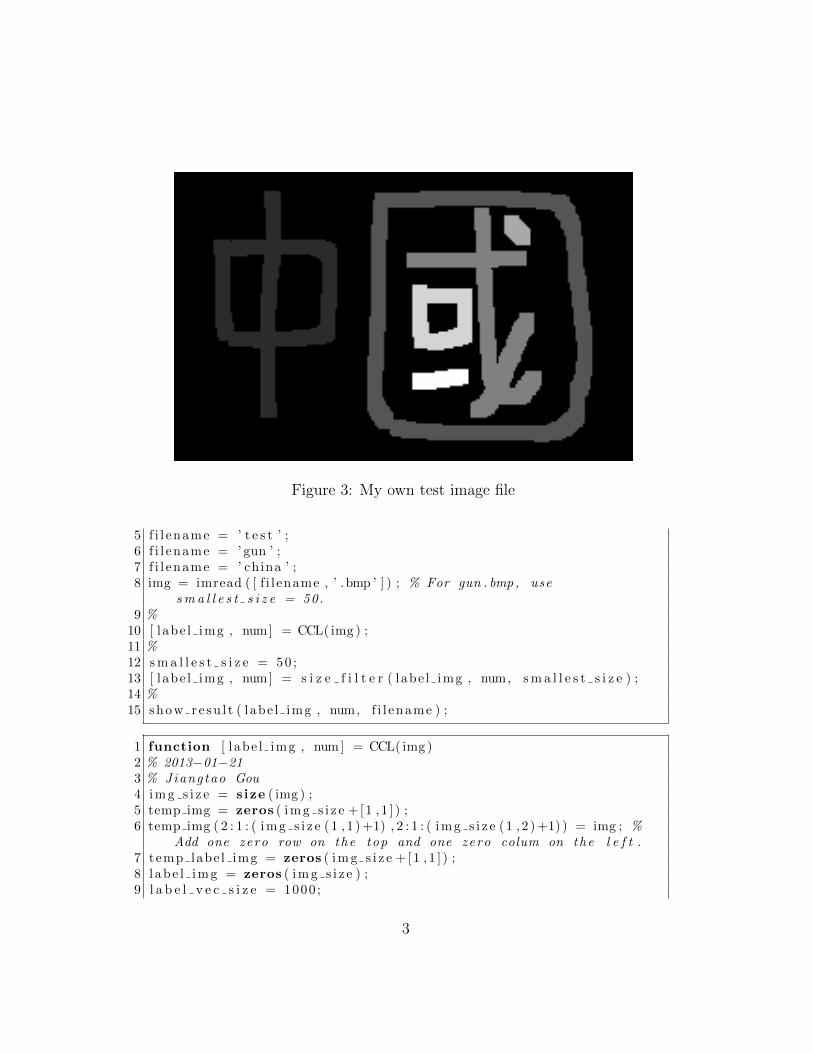
Figure 3: My own test image file
5 f i l ename = ’ t e s t ’ ;6 f i l ename = ’ gun ’ ;7 f i l ename = ’ china ’ ;8 img = imread ( [ f i l ename , ’ .bmp ’ ] ) ; % For gun . bmp , use
sm a l l e s t s i z e = 50.9 %
10 [ labe l img , num] = CCL( img ) ;11 %12 sma l l e s t s i z e = 50 ;13 [ l abe l img , num] = s i z e f i l t e r ( labe l img , num, sma l l e s t s i z e ) ;14 %15 show re su l t ( l abe l img , num, f i l ename ) ;
1 function [ l abe l img , num] = CCL( img )2 % 2013−01−213 % Jiangtao Gou4 img s i z e = s ize ( img ) ;5 temp img = zeros ( img s i z e + [1 , 1 ] ) ;6 temp img ( 2 : 1 : ( img s i z e (1 , 1 )+1) , 2 : 1 : ( img s i z e (1 , 2 )+1) ) = img ; %
Add one zero row on the top and one zero colum on the l e f t .7 temp labe l img = zeros ( img s i z e + [1 , 1 ] ) ;8 l abe l img = zeros ( img s i z e ) ;9 l a b e l v e c s i z e = 1000 ;
3
10 l a b e l v e c = 1 : 1 : l a b e l v e c s i z e ;11 num = 0 ;12 l a b e l = 0 ;13 for u = 2 : 1 : ( img s i z e (1 , 1 )+1)14 for v = 2 : 1 : ( img s i z e (1 , 2 )+1)15 i f temp img (u , v ) == 116 uppe r l abe l = temp labe l img (u−1,v ) ; % Upper l a b e l17 l e f t l a b e l = temp labe l img (u , v−1) ; % Le f t l a b e l18 i f ( uppe r l abe l == l e f t l a b e l ) && ( uppe r l abe l ˜= 0)
&& ( l e f t l a b e l ˜= 0) % The same l a b e l19 temp labe l img (u , v ) = uppe r l abe l ;20 e l s e i f ( uppe r l abe l ˜= l e f t l a b e l ) && ˜( uppe r l abe l
&& l e f t l a b e l ) % Either i s 021 temp labe l img (u , v ) = max( upper l abe l , l e f t l a b e l
) ;22 e l s e i f ( uppe r l abe l ˜= l e f t l a b e l ) && ( uppe r l abe l >
0) && ( l e f t l a b e l > 0) % Both23 temp labe l img (u , v ) = min( upper l abe l , l e f t l a b e l
) ;24 l a b e l v e c = E tab le ( l abe l , l ab e l v e c ,
upper l abe l , l e f t l a b e l ) ;25 else26 l a b e l = l a b e l + 1 ;27 temp labe l img (u , v ) = l a b e l ;28 i f l a b e l > l a b e l v e c s i z e29 error ( ’The S i z e o f Equiva lent Table i s NOT
big enough . Please In c r ea s e i t . ’ ) ;30 end31 end32 end33 end34 end35 l abe l img = temp labe l img ( 2 : 1 : ( img s i z e (1 , 1 )+1) , 2 : 1 : ( img s i z e
(1 , 2 )+1) ) ;36 l a b e l v e c = l a b e l v e c ( 1 : 1 : l a b e l ) ;37 un i qu e l ab e l = unique ( l a b e l v e c ) ;38 for u = 1 : 1 : img s i z e (1 , 1 )39 for v = 1 : 1 : img s i z e (1 , 2 )40 i f img (u , v ) == 141 l abe l img (u , v ) = l a b e l v e c ( l abe l img (u , v ) ) ; % Merger
Regions42 l abe l img (u , v ) = find ( un i qu e l ab e l == labe l img (u , v )
) ; % Use 1 , 2 , 3 , . . . as the reg ion numbers .43 end44 end
4
45 end46 num = length ( un i qu e l ab e l ) ;
1 function l a b e l v e c = E tab le ( l abe l , l ab e l v e c , L u , L l )2 % 2013−01−213 % Jiangtao Gou4 min L = min( l a b e l v e c ( L u ) , l a b e l v e c ( L l ) ) ;5 i f ( l a b e l v e c ( L u ) == L u ) && ( l a b e l v e c ( L l ) == L l ) % Nei ther
o f indexes has been changed6 l a b e l v e c ( L u ) = min L ;7 l a b e l v e c ( L l ) = min L ;8 else9 for i =1:1 : l a b e l
10 i f ( l a b e l v e c ( i ) == l a b e l v e c ( L u ) ) | | ( l a b e l v e c ( i ) ==l a b e l v e c ( L l ) )
11 l a b e l v e c ( i ) = min L ;12 end13 end14 end
1 function [ l abe l img , num] = s i z e f i l t e r ( labe l img , num,sma l l e s t s i z e )
2 % 2013−01−223 % Jiangtao Gou4 img s i z e = s ize ( l abe l img ) ;5 p i x e l p o i n t c oun t e r = zeros (1 ,num) ;6 for i =1:1 :num7 p i x e l p o i n t c oun t e r ( i ) = length ( find ( l abe l img == i ) ) ;8 end9 i f sum( p i x e l p o i n t c oun t e r < sm a l l e s t s i z e )
10 n o t n o i s e l a b e l = ( p i x e l p o i n t c oun t e r >= sma l l e s t s i z e ) ;11 n o t n o i s e l a b e l l o c = find ( n o t n o i s e l a b e l > 0) ;12 for u = 1 : 1 : img s i z e (1 , 1 )13 for v = 1 : 1 : img s i z e (1 , 2 )14 i f l abe l img (u , v ) > 015 i f n o t n o i s e l a b e l ( l abe l img (u , v ) ) == 016 l abe l img (u , v ) = 0 ;17 else18 l abe l img (u , v ) = find ( n o t n o i s e l a b e l l o c ==
labe l img (u , v ) ) ;19 end20 end21 end22 end23 else
5
24 n o t n o i s e l a b e l l o c = ones ( s ize ( p i x e l p o i n t c oun t e r ) ) ;25 end26 num = length ( n o t n o i s e l a b e l l o c ) ;
1 function show re su l t ( l abe l img , num, f i l ename )2 % 2013−01−223 % Jiangtao Gou4 img s i z e = s ize ( l abe l img ) ;5 gray img = labe l img ;6 for u = 1 : 1 : img s i z e (1 , 1 )7 for v = 1 : 1 : img s i z e (1 , 2 )8 i f l abe l img (u , v ) > 09 gray img (u , v ) = round( l abe l img (u , v ) /num∗255) ;
10 end11 end12 end13 imshow( gray img , [ 0 255 ] ) ;14 set ( gcf , ’ p ape r s i z e ’ , [ 5 5 ] ) ;15 picname = [ ’mp1 ’ , f i l ename , ’ . eps ’ ] ;16 saveas ( gcf , picname , ’ epsc ’ ) ;17 eps2pdf ( picname ) ;
6
Winter 2013 EECS 332 Digital Image Analysis
Machine Problem 2Morphological Operators
Jiangtao GouDepartment of Statistics, Northwestern University
Instructor: Prof. Ying Wu
24 January 2013
1 Introduction
In this report, I realized some basic morphological operators which wereintroduction on January 17th. By following slides ”Binary Image AnalysisIII” by Prof Wu, and Jain, Kasturi and Schunck’s ”Machine Vision” (1995),page 61-69, the following morphological operators are defined below.
ErosionAB = {p|Bp ⊆ A}. (1)
DilationA⊕B = ∪bi∈BAbi . (2)
OpeningA ◦B = (AB)⊕B. (3)
ClosingA •B = (A⊕B)B. (4)
BoundaryβB(A) = A− (AB) . (5)
In order to get clear boundary, I tried to combine those morphologicaloperators above. In the end, this one below worked well, and I called it”Clear Boundary”, as shown below.
Clear Boundary
γB(A) = (A⊕B)− (AB) . (6)
Meanwhile, in order to get rid of the noise, I used the techniques inMachine Problem 1, where I labelled different component, and treated thesmall components as noise.
1
2 Algorithm Description
For erosion and dilation, I went through the whole picture, and decidedthe output image.
For opening, closing, boundary, and clear boundary, I simply used thecombination of erosion and dilation.
In order to get rid of the noise, I ran the size filter at first, then I ranclear boundary function. The threshold need to be specified ahead.
3 Results analysis
First, I tried to apply a 3 by 3 square structure element (Figure 1) ongun.bmp.
Figure 1: Structure Element: 3 by 3 Square
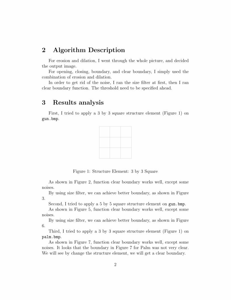
As shown in Figure 2, function clear boundary works well, except somenoises.
By using size filter, we can achieve better boundary, as shown in Figure3.
Second, I tried to apply a 5 by 5 square structure element on gun.bmp.As shown in Figure 5, function clear boundary works well, except some
noises.By using size filter, we can achieve better boundary, as shown in Figure
6.Third, I tried to apply a 3 by 3 square structure element (Figure 1) on
palm.bmp.As shown in Figure 7, function clear boundary works well, except some
noises. It looks that the boundary in Figure 7 for Palm was not very clear.We will see by change the structure element, we will get a clear boundary.
2
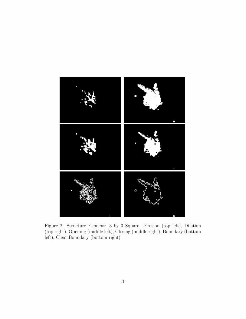
Figure 2: Structure Element: 3 by 3 Square. Erosion (top left), Dilation(top right), Opening (middle left), Closing (middle right), Boundary (bottomleft), Clear Boundary (bottom right)
3
Figure 3: Structure Element: 3 by 3 Square. Clear Boundary after Filtering.Threshold = 9 (left), Threshold = 100 (right)
Figure 4: Structure Element: 5 by 5 Square
4

Figure 5: Structure Element: 5 by 5 Square. Erosion (top left), Dilation(top right), Opening (middle left), Closing (middle right), Boundary (bottomleft), Clear Boundary (bottom right)
5
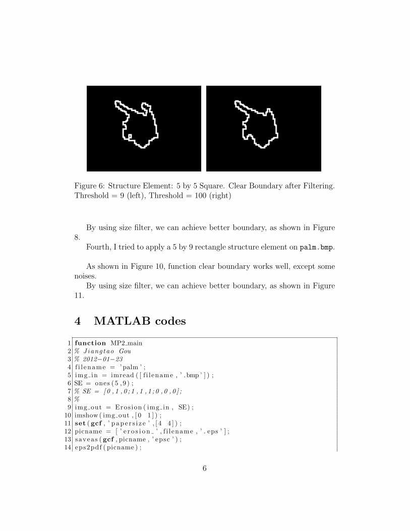
Figure 6: Structure Element: 5 by 5 Square. Clear Boundary after Filtering.Threshold = 9 (left), Threshold = 100 (right)
By using size filter, we can achieve better boundary, as shown in Figure8.
Fourth, I tried to apply a 5 by 9 rectangle structure element on palm.bmp.
As shown in Figure 10, function clear boundary works well, except somenoises.
By using size filter, we can achieve better boundary, as shown in Figure11.
4 MATLAB codes
1 function MP2 main2 % Jiangtao Gou3 % 2012−01−234 f i l ename = ’palm ’ ;5 img in = imread ( [ f i l ename , ’ .bmp ’ ] ) ;6 SE = ones (5 , 9 ) ;7 % SE = [0 , 1 , 0 ; 1 , 1 , 1 ; 0 , 0 , 0 ] ;8 %9 img out = Eros ion ( img in , SE) ;
10 imshow( img out , [ 0 1 ] ) ;11 set ( gcf , ’ p ape r s i z e ’ , [ 4 4 ] ) ;12 picname = [ ’ e r o s i o n ’ , f i l ename , ’ . eps ’ ] ;13 saveas ( gcf , picname , ’ epsc ’ ) ;14 eps2pdf ( picname ) ;
6
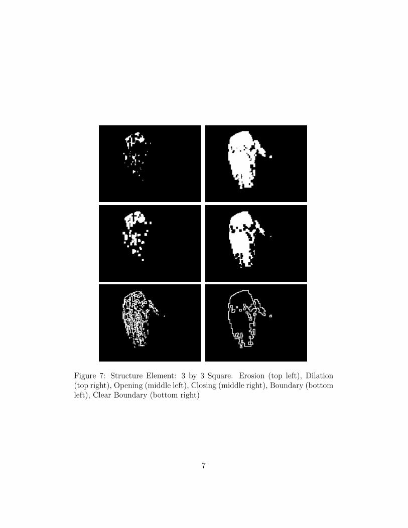
Figure 7: Structure Element: 3 by 3 Square. Erosion (top left), Dilation(top right), Opening (middle left), Closing (middle right), Boundary (bottomleft), Clear Boundary (bottom right)
7
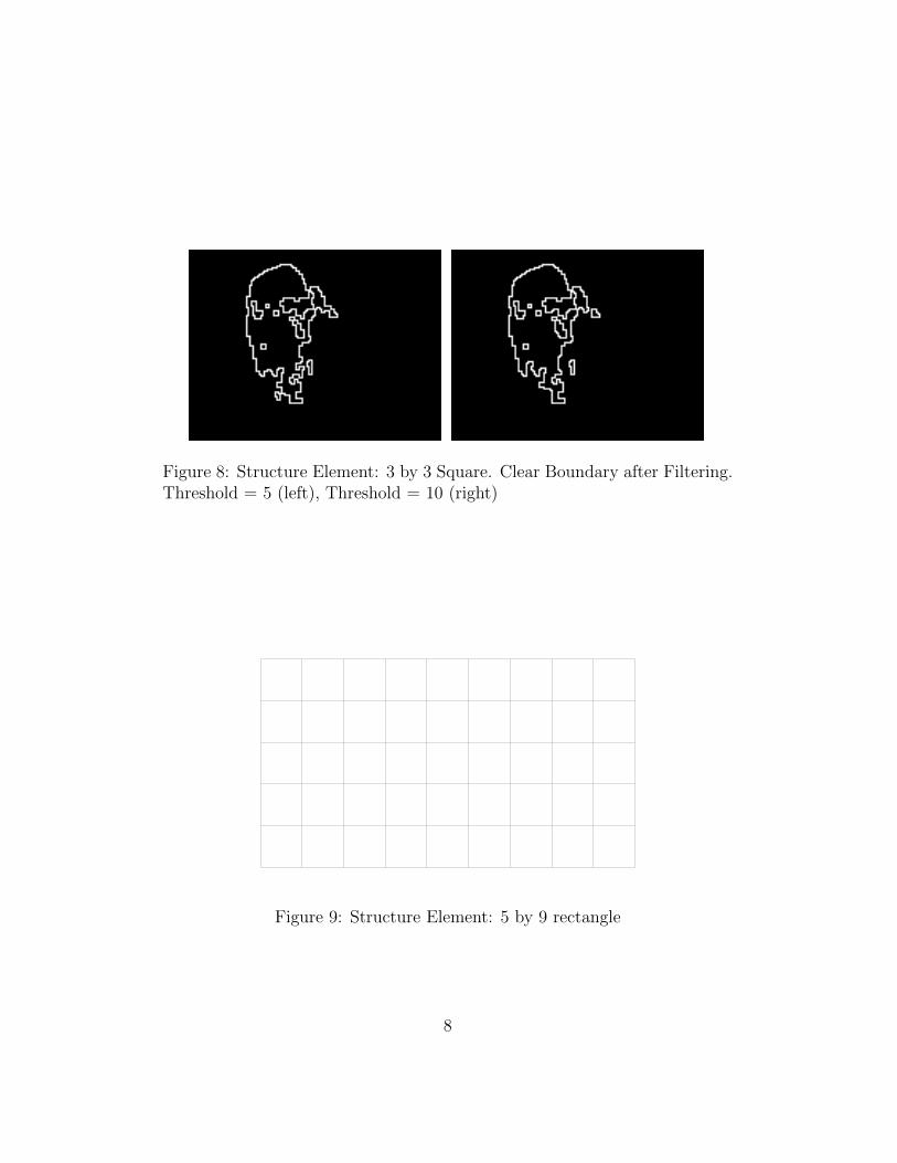
Figure 8: Structure Element: 3 by 3 Square. Clear Boundary after Filtering.Threshold = 5 (left), Threshold = 10 (right)
Figure 9: Structure Element: 5 by 9 rectangle
8
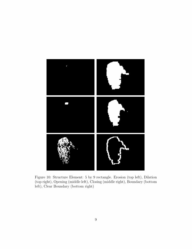
Figure 10: Structure Element: 5 by 9 rectangle. Erosion (top left), Dilation(top right), Opening (middle left), Closing (middle right), Boundary (bottomleft), Clear Boundary (bottom right)
9
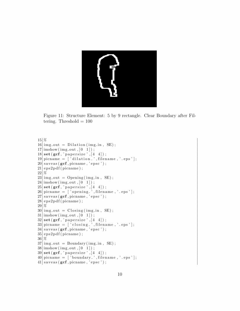
Figure 11: Structure Element: 5 by 9 rectangle. Clear Boundary after Fil-tering. Threshold = 100
15 %16 img out = Di l a t i on ( img in , SE) ;17 imshow( img out , [ 0 1 ] ) ;18 set ( gcf , ’ p ape r s i z e ’ , [ 4 4 ] ) ;19 picname = [ ’ d i l a t i o n ’ , f i l ename , ’ . eps ’ ] ;20 saveas ( gcf , picname , ’ epsc ’ ) ;21 eps2pdf ( picname ) ;22 %23 img out = Opening ( img in , SE) ;24 imshow( img out , [ 0 1 ] ) ;25 set ( gcf , ’ p ape r s i z e ’ , [ 4 4 ] ) ;26 picname = [ ’ opening ’ , f i l ename , ’ . eps ’ ] ;27 saveas ( gcf , picname , ’ epsc ’ ) ;28 eps2pdf ( picname ) ;29 %30 img out = Clos ing ( img in , SE) ;31 imshow( img out , [ 0 1 ] ) ;32 set ( gcf , ’ p ape r s i z e ’ , [ 4 4 ] ) ;33 picname = [ ’ c l o s i n g ’ , f i l ename , ’ . eps ’ ] ;34 saveas ( gcf , picname , ’ epsc ’ ) ;35 eps2pdf ( picname ) ;36 %37 img out = Boundary ( img in , SE) ;38 imshow( img out , [ 0 1 ] ) ;39 set ( gcf , ’ p ape r s i z e ’ , [ 4 4 ] ) ;40 picname = [ ’ boundary ’ , f i l ename , ’ . eps ’ ] ;41 saveas ( gcf , picname , ’ epsc ’ ) ;
10
42 eps2pdf ( picname ) ;43 %44 img temp = Di l a t i on ( img in , SE) ;45 img out = Boundary ( img temp , SE) ;46 imshow( img out , [ 0 1 ] ) ;47 set ( gcf , ’ p ape r s i z e ’ , [ 4 4 ] ) ;48 picname = [ ’ c learBoundary ’ , f i l ename , ’ . eps ’ ] ;49 saveas ( gcf , picname , ’ epsc ’ ) ;50 eps2pdf ( picname ) ;51 %52 % F i l t e r i n g at f i r s t53 img = imread ( [ f i l ename , ’ .bmp ’ ] ) ; % For gun . bmp , use
sm a l l e s t s i z e = 50.54 [ labe l img , num] = CCL( img ) ;55 sm a l l e s t s i z e = 100 ;56 [ l abe l img , num] = s i z e f i l t e r ( labe l img , num, sma l l e s t s i z e ) ;57 s i z e img = s ize ( l abe l img ) ;58 img in = labe l img59 for i = 1 : 1 : s i z e img (1 , 1 )60 for j = 1 : 1 : s i z e img (1 , 2 )61 i f l abe l img ( i , j ) > 062 img in ( i , j ) = 1 ;63 end64 end65 end66 img temp = Di l a t i on ( img in , SE) ;67 img out = Boundary ( img temp , SE) ;68 imshow( img out , [ 0 1 ] ) ;69 set ( gcf , ’ p ape r s i z e ’ , [ 4 4 ] ) ;70 picname = [ ’ f i l t e rBounda ry ’ , f i l ename , ’ . eps ’ ] ;71 saveas ( gcf , picname , ’ epsc ’ ) ;72 eps2pdf ( picname ) ;
1 function img out = Eros ion ( img in , SE)2 % Note : SEs s i d e l e n g t h s shou ld be odd numbers , e . g . , 3by3 , 1by3
, 5by7 . . .3 % Jiangtao Gou4 % 2012−01−235 s i z e SE = s ize (SE) ;6 extenderR = ( s i z e SE (1 , 2 )−1) /2 ;7 extenderC = ( s i z e SE (1 , 1 )−1) /2 ;8 s i z e img = s ize ( img in ) ;9 img out = zeros ( s ize ( img in ) ) ;
10 for i = ( extenderC+1) : 1 : ( s i z e img (1 , 1 )−extenderC )11 for j = ( extenderR+1) : 1 : ( s i z e img (1 , 2 )−extenderR )
11
12 i f sum(sum( img in ( ( i−extenderC ) : 1 : ( i+extenderC ) , ( j−extenderR ) : 1 : ( j+extenderR ) ) .∗SE) ) == sum(sum(SE) )
13 img out ( i , j ) = 1 ;14 else15 img out ( i , j ) = 0 ;16 end17 end18 end19 % Test data20 % img in = [0 , 0 , 1 , 0 , 0 ; 0 , 1 , 1 , 1 , 0 ; 0 , 0 , 1 , 0 , 0 ; 0 , 1 , 1 , 1 , 1 ; 0 , 0 , 0 , 0 , 0 ] ;21 % SE = [ 1 , 1 , 1 ] ;
1 function img out = Di l a t i on ( img in , SE)2 % Note : SEs s i d e l e n g t h s shou ld be odd numbers , e . g . , 3by3 , 1by3
, 5by7 . . .3 % Jiangtao Gou4 % 2012−01−235 s i z e SE = s ize (SE) ;6 extenderR = ( s i z e SE (1 , 2 )−1) /2 ;7 extenderC = ( s i z e SE (1 , 1 )−1) /2 ;8 s i z e img = s ize ( img in ) ;9 img out temp = zeros ( s ize ( img in )+[2∗ extenderC ,2∗ extenderR ] ) ;
10 for i = ( extenderC+1) : 1 : ( s i z e img (1 , 1 )+extenderC )11 for j = ( extenderR+1) : 1 : ( s i z e img (1 , 2 )+extenderR )12 i f img in ( i−extenderC , j−extenderR ) == 113 for k1 = 1 : 1 : s i z e SE (1 , 1 )14 for k2 = 1 : 1 : s i z e SE (1 , 2 )15 i f SE(k1 , k2 ) == 116 img out temp ( i+k1−extenderC−1, j+k2−
extenderR−1) = 1 ;17 end18 end19 end20 end21 end22 end23 img out = img out temp ( ( extenderC+1) : 1 : ( s i z e img (1 , 1 )+extenderC )
, ( extenderR+1) : 1 : ( s i z e img (1 , 2 )+extenderR ) ) ;
1 function img out = Opening ( img in , SE)2 % Note : SEs s i d e l e n g t h s shou ld be odd numbers3 % Jiangtao Gou4 % 2012−01−235 img temp = Eros ion ( img in , SE) ;6 img out = Di l a t i on ( img temp ,SE) ;
12
1 function img out = Clos ing ( img in , SE)2 % Note : SEs s i d e l e n g t h s shou ld be odd numbers3 % Jiangtao Gou4 % 2012−01−235 img temp = Di l a t i on ( img in , SE) ;6 img out = Eros ion ( img temp , SE) ;
1 function img out = Boundary ( img in , SE)2 % Note : SEs s i d e l e n g t h s shou ld be odd numbers3 % Jiangtao Gou4 % 2012−01−235 img temp = Eros ion ( img in , SE) ;6 img out = img in − img temp ;
13
Winter 2013 EECS 332 Digital Image Analysis
Machine Problem 3Histogram Techniques
Jiangtao GouDepartment of Statistics, Northwestern University
Instructor: Prof. Ying Wu
27 January 2013
1 Introduction
In this report, I implied the histogram equalization and the lighting cor-rection to adjust the gray scale of pictures, and made it easy to be distin-guished by human eyes.
Histogram equalization is a technique to stretch the histogram of the pix-els’ grayscale, and make the histogram as uniform as possible. In statistics,when a p-value is used as a test statistic for a simple null hypothesis, thenfor any continuously distributed test statistic, the p-value is uniformly dis-tributed between 0 and 1 if the null hypothesis is true. Similarly, histogramequalization normalizes the original grayscale histogram at first, then usesthe distribution function as the new variables, and scales the new variablebetween 0 and 255 to form a new histogram. This histogram is approximatelyuniformly distribution. A new picture is got correspondingly.
Lighting correction is used to set the brightness all over a certain pictureto a nearly same level. By treating the grayscale as a function of the positionof pixels, a plan and quadratic surface can be estimated as the background.By submitting the background from the original picture, we will get a lightingcorrection. In application, I added the median of the estimated backgroundsurface back, and then either used truncation technique, where I set all num-ber bigger than 255 as 255 and all number smaller than 0 as 0, or used scaletechnique, where I set the biggest number as 255 and smallest number as 0,then all other number were determined linearly by linear interpolation.
1
2 Algorithm Description
Code in HistoEqualization.m is for histogram equalization, where ahistogram of original picture is constructed at first, then the grayscale isstretched in order to make the new histogram approximately uniform.
Code in LightingCorrection.m calls either LightingCorrectionLinear.mor LightingCorrectionQuadratic.m.
Code in LightingCorrectionLinear.m applies a linear lighting correc-tion. First a plane is estimated by using the least square estimation toestimate a, b and const.
P (R,C) = aR + bC + const. (1)
Then get the correction CGp(R,C) this way.
CGp(R,C) = G(R,C)− P (R,C) + medianR,C (P (R,C)) . (2)
In the end, either a truncated version
CGpt(R,C) =
0, if CGp(R,C) < 0,
CGp(R,C), if 0 ≤ CGp(R,C) ≤ 255,
255, if CGp(R,C) > 255,
(3)
or a scaled version
CGps(R,C) = 255 · CGp(R,C)−minCGp(R,C)
maxCGp(R,C)−minCGp(R,C)(4)
gives the corrected pictures.Similarly, code in LightingCorrectionQuadratic.m applies a quadratic
lighting correction. First a quadratic surface is estimated by using the leastsquare estimation to estimate a, b, c, d, e and const.
S(R,C) = aR2 + bRC + cC2 + dR + eC + const. (5)
Then get the correction CGs(R,C) by using the formula below.
CGs(R,C) = G(R,C)− S(R,C) + medianR,C (S(R,C)) . (6)
In the end, either a truncated version
CGst(R,C) =
0, if CGs(R,C) < 0,
CGs(R,C), if 0 ≤ CGs(R,C) ≤ 255,
255, if CGs(R,C) > 255,
(7)
2
or a scaled version
CGss(R,C) = 255 · CGs(R,C)−minCGs(R,C)
maxCGs(R,C)−minCGs(R,C)(8)
gives the pictures after correction.
3 Results analysis
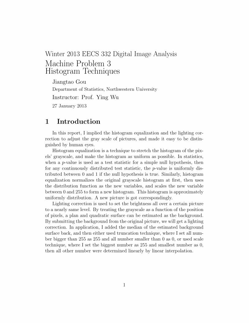
Figure 1 shows the original moon.bmp and its Histogram.
0 50 100 150 200 2500
0.01
0.02
0.03
0.04
0.05
0.06
0.07
0.08
Gray Scale
Den
sity
Figure 1: The original moon.bmp and its Histogram.
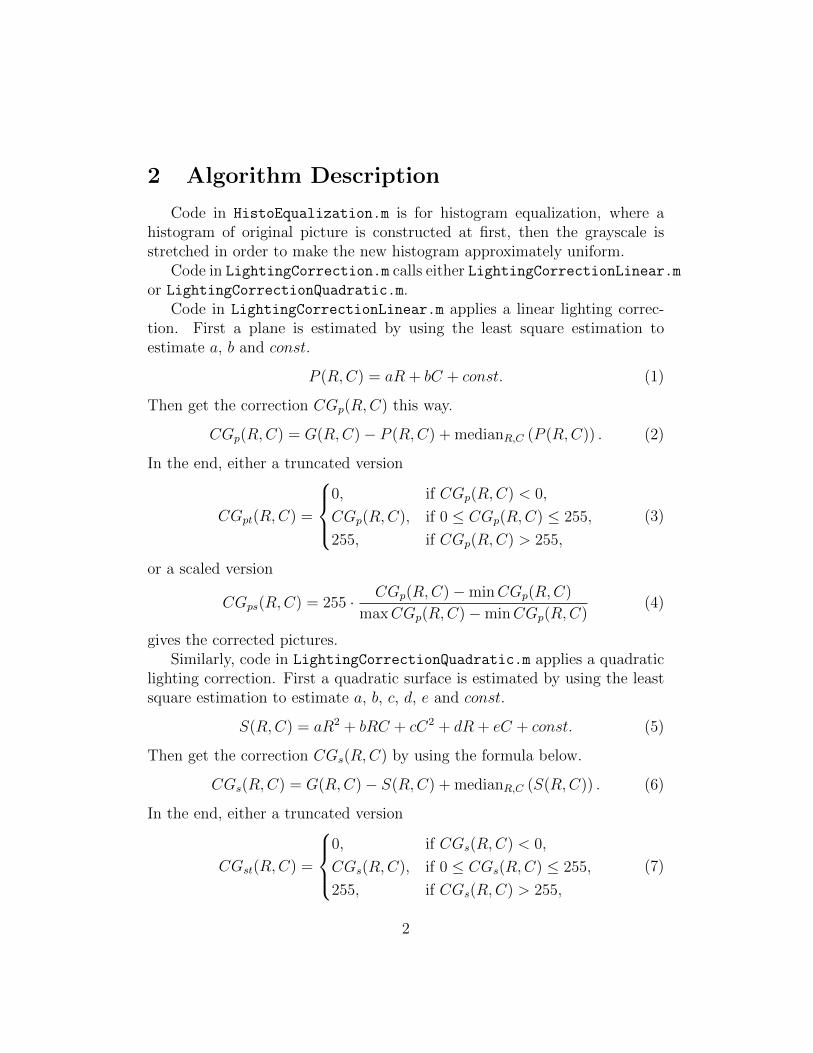
Figure 2 represents the distribution function and the transformation ofmoon.bmp.
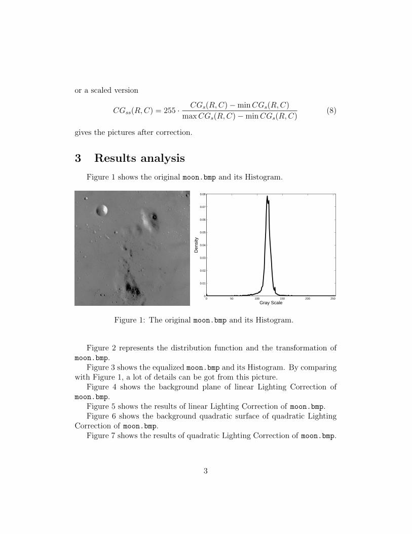
Figure 3 shows the equalized moon.bmp and its Histogram. By comparingwith Figure 1, a lot of details can be got from this picture.
Figure 4 shows the background plane of linear Lighting Correction ofmoon.bmp.
Figure 5 shows the results of linear Lighting Correction of moon.bmp.Figure 6 shows the background quadratic surface of quadratic Lighting
Correction of moon.bmp.Figure 7 shows the results of quadratic Lighting Correction of moon.bmp.
3
0 50 100 150 200 2500
0.1
0.2
0.3
0.4
0.5
0.6
0.7
0.8
0.9
1
Gray Scale
Dis
trib
utio
n F
unct
ion
Figure 2: Distribution Function and the Transformation of moon.bmp.
0 50 100 150 200 2500
0.01
0.02
0.03
0.04
0.05
0.06
0.07
0.08
Gray Scale
Den
sity
Figure 3: The equalized moon.bmp and its Histogram.
4
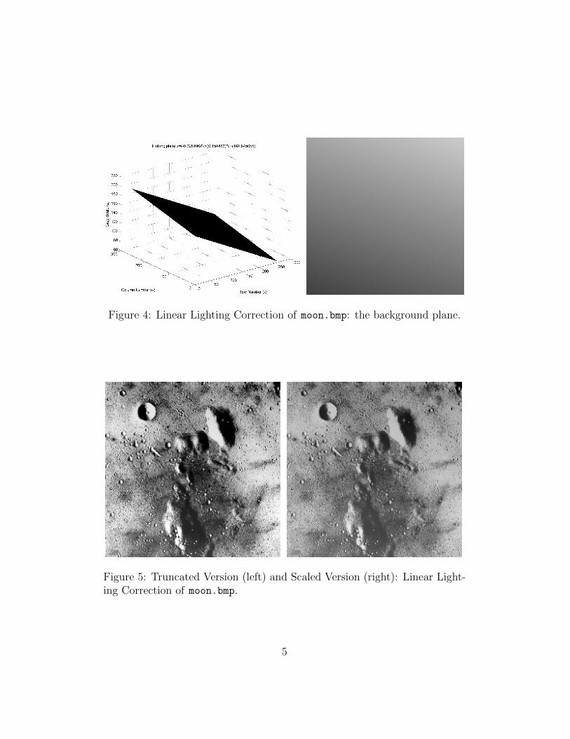
Figure 4: Linear Lighting Correction of moon.bmp: the background plane.
Figure 5: Truncated Version (left) and Scaled Version (right): Linear Light-ing Correction of moon.bmp.
5
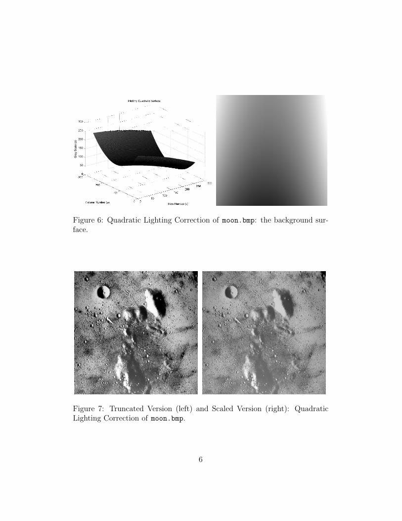
Figure 6: Quadratic Lighting Correction of moon.bmp: the background sur-face.
Figure 7: Truncated Version (left) and Scaled Version (right): QuadraticLighting Correction of moon.bmp.
6
By comparing with Figure 3, pictures in Figure 5 and Figure 7 have moreuniformly distributed grayscales.
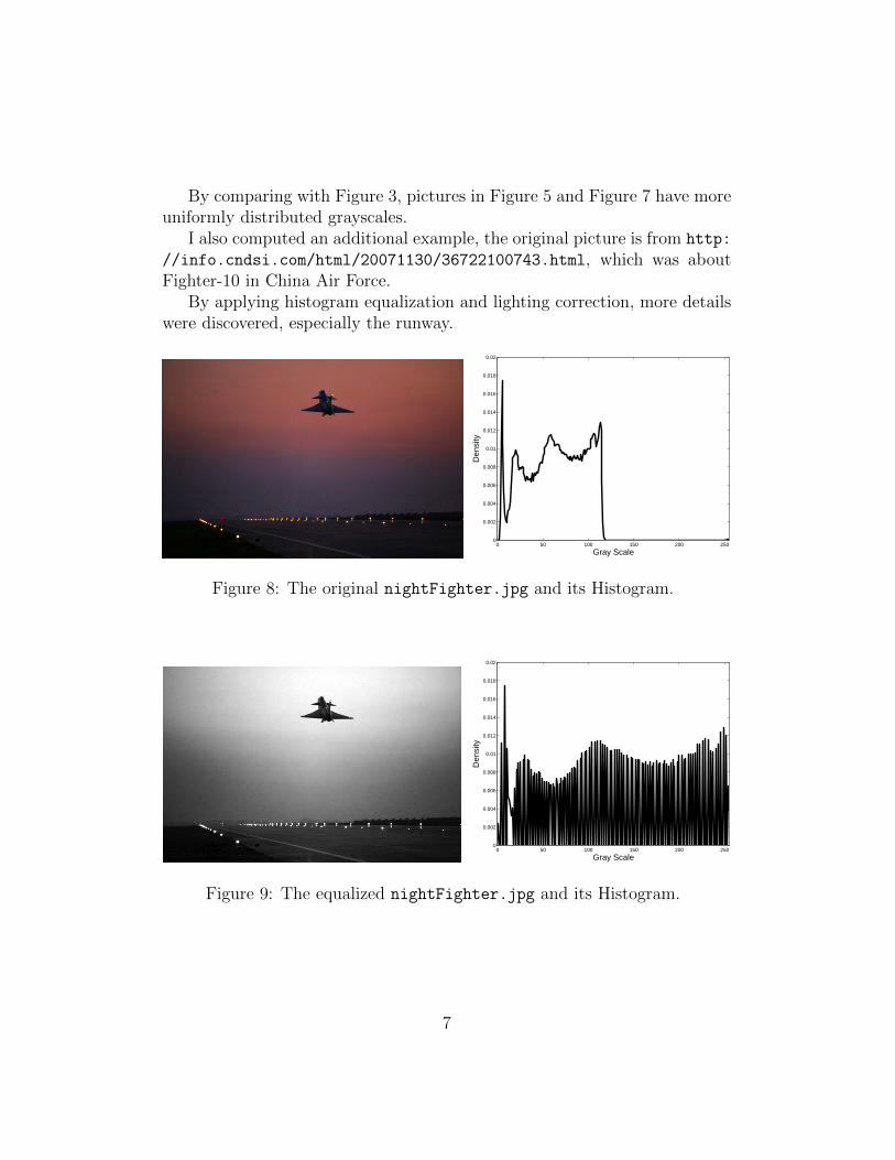
I also computed an additional example, the original picture is from http:
//info.cndsi.com/html/20071130/36722100743.html, which was aboutFighter-10 in China Air Force.
By applying histogram equalization and lighting correction, more detailswere discovered, especially the runway.
0 50 100 150 200 2500
0.002
0.004
0.006
0.008
0.01
0.012
0.014
0.016
0.018
0.02
Gray Scale
Den
sity
Figure 8: The original nightFighter.jpg and its Histogram.
0 50 100 150 200 2500
0.002
0.004
0.006
0.008
0.01
0.012
0.014
0.016
0.018
0.02
Gray Scale
Den
sity
Figure 9: The equalized nightFighter.jpg and its Histogram.
7
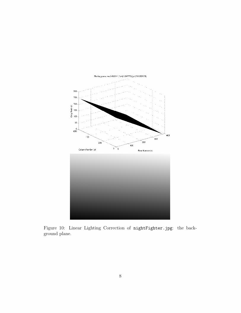
Figure 10: Linear Lighting Correction of nightFighter.jpg: the back-ground plane.
8
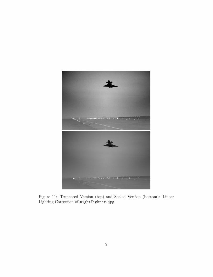
Figure 11: Truncated Version (top) and Scaled Version (bottom): LinearLighting Correction of nightFighter.jpg.
9
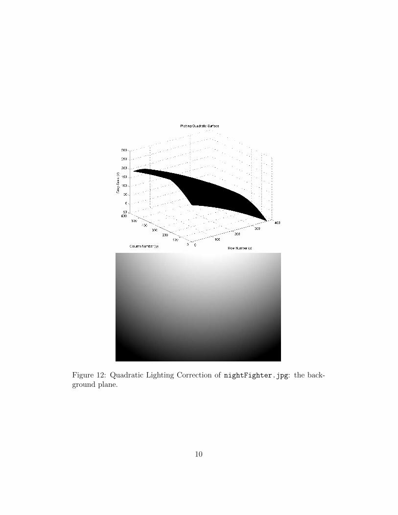
Figure 12: Quadratic Lighting Correction of nightFighter.jpg: the back-ground plane.
10
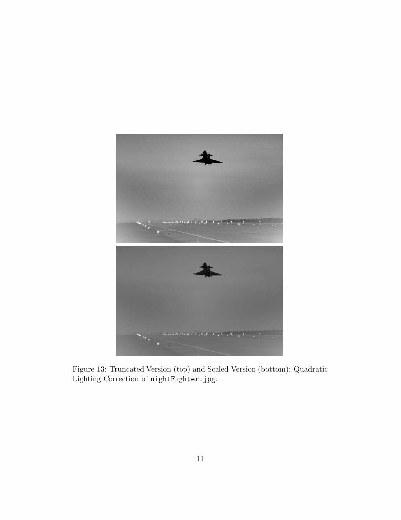
Figure 13: Truncated Version (top) and Scaled Version (bottom): QuadraticLighting Correction of nightFighter.jpg.
11
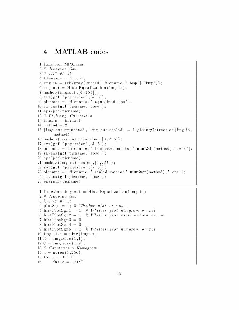
4 MATLAB codes
1 function MP3 main2 % Jiangtao Gou3 % 2013−01−254 f i l ename = ’moon ’ ;5 img in = rgb2gray ( imread ( [ f i l ename , ’ .bmp ’ ] , ’bmp ’ ) ) ;6 img out = Hi s toEqua l i z a t i on ( img in ) ;7 imshow ( img out , [ 0 , 2 5 5 ] ) ;8 set ( gcf , ’ p ape r s i z e ’ , [ 5 5 ] ) ;9 picname = [ f i l ename , ’ e qua l i z e d . eps ’ ] ;
10 saveas ( gcf , picname , ’ epsc ’ ) ;11 eps2pdf ( picname ) ;12 % Ligh t ing Correct ion13 img in = img out ;14 method = 2 ;15 [ img out truncated , img out s ca l ed ] = L ight ingCor r ec t i on ( img in ,
method ) ;16 imshow( img out truncated , [ 0 , 2 5 5 ] ) ;17 set ( gcf , ’ p ape r s i z e ’ , [ 5 5 ] ) ;18 picname = [ f i l ename , ’ truncated method ’ ,num2str(method ) , ’ . eps ’ ] ;19 saveas ( gcf , picname , ’ epsc ’ ) ;20 eps2pdf ( picname ) ;21 imshow( img out sca l ed , [ 0 , 2 5 5 ] ) ;22 set ( gcf , ’ p ape r s i z e ’ , [ 5 5 ] ) ;23 picname = [ f i l ename , ’ sca led method ’ ,num2str(method ) , ’ . eps ’ ] ;24 saveas ( gcf , picname , ’ epsc ’ ) ;25 eps2pdf ( picname ) ;
1 function img out = Hi s toEqua l i z a t i on ( img in )2 % Jiangtao Gou3 % 2013−01−254 plotSgn = 1 ; % Whether p l o t or not5 h i s tP lotSgn1 = 1 ; % Whether p l o t h is tgram or not6 h i s tP lotSgn2 = 1 ; % Whether p l o t d i s t r i b u t i o n or not7 h i s tP lotSgn3 = 0 ;8 h i s tP lotSgn4 = 0 ;9 h i s tP lotSgn5 = 1 ; % Whether p l o t h is tgram or not
10 img s i z e = s ize ( img in ) ;11 R = img s i z e (1 , 1 ) ;12 C = img s i z e (1 , 2 ) ;13 % Construct a Histogram14 h = zeros (1 ,256) ;15 for r = 1 : 1 :R16 for c = 1 : 1 :C
12
17 h( img in ( r , c )+1) = h( img in ( r , c )+1)+1;18 end19 end20 x = 0 : 1 : 2 5 5 ;21 y1 = h ;22 y2 = 1/sum(h) ∗h ;23 i f plotSgn && his tP lotSgn124 plot (x , y2 , ’−k ’ , ’ LineWidth ’ , 3 ) ;25 axis ( [ 0 255 0 0 . 0 8 ] ) ;26 xlabel ( ’Gray Sca l e ’ , ’ f o n t s i z e ’ , 16) ;27 ylabel ( ’ Density ’ , ’ f o n t s i z e ’ , 16) ;28 set ( gcf , ’ p ape r s i z e ’ , [ 5 8 ] ) ;29 picname = [ ’ h i s t o r i g i n a l . eps ’ ] ;30 saveas ( gcf , picname , ’ epsc ’ ) ;31 eps2pdf ( picname ) ;32 end33 %x = reshape ( img in , R∗C,1 ) ; [ f , x i ] = k s d en s i t y ( x ) ; p l o t ( xi , f ) ;34 y3 = zeros ( s ize ( y2 ) ) ;35 y3 (1 ) = y2 (1 ) ;36 for i =2:1 : length (h)37 y3 ( i ) = y3 ( i −1)+y2 ( i ) ;38 end39 i f plotSgn && his tP lotSgn240 plot (x , y3 , ’−k ’ , ’ LineWidth ’ , 3 ) ;41 axis ( [ 0 255 0 1 ] ) ;42 xlabel ( ’Gray Sca l e ’ , ’ f o n t s i z e ’ , 16) ;43 ylabel ( ’ D i s t r i bu t i on Function ’ , ’ f o n t s i z e ’ , 16) ;44 set ( gcf , ’ p ape r s i z e ’ , [ 5 8 ] ) ;45 picname = [ ’ d i s t r o r i g i n a l . eps ’ ] ;46 saveas ( gcf , picname , ’ epsc ’ ) ;47 eps2pdf ( picname ) ;48 end49 x2 = round( y3 ∗255) ;50 i f plotSgn && his tP lotSgn351 plot ( x2 , y2 , ’−r ’ , ’ LineWidth ’ , 3 ) ;52 axis ( [ 0 255 0 0 . 0 8 ] ) ;53 xlabel ( ’Gray Sca l e ’ , ’ f o n t s i z e ’ , 16) ;54 ylabel ( ’ Density ’ , ’ f o n t s i z e ’ , 16) ;55 set ( gcf , ’ p ape r s i z e ’ , [ 5 8 ] ) ;56 picname = [ ’ h i s t e q u a l i z e d t r y . eps ’ ] ;57 saveas ( gcf , picname , ’ epsc ’ ) ;58 eps2pdf ( picname ) ;59 end60 i f plotSgn && his tP lotSgn461 plot ( x2 , y3 , ’−r ’ , ’ LineWidth ’ , 3 ) ;
13
62 axis ( [ 0 255 0 1 ] ) ;63 xlabel ( ’Gray Sca l e ’ , ’ f o n t s i z e ’ , 16) ;64 ylabel ( ’ D i s t r i bu t i on Function ’ , ’ f o n t s i z e ’ , 16) ;65 set ( gcf , ’ p ape r s i z e ’ , [ 5 8 ] ) ;66 picname = [ ’ d i s t r e q u a l i z e d . eps ’ ] ;67 saveas ( gcf , picname , ’ epsc ’ ) ;68 eps2pdf ( picname ) ;69 end70 for r = 1 : 1 :R71 for c = 1 : 1 :C72 img out ( r , c ) = x2 ( img in ( r , c )+1) ;73 end74 end75 % Construct an Equa l i z ed Histogram76 hh = zeros (1 ,256) ;77 for r = 1 : 1 :R78 for c = 1 : 1 :C79 hh( img out ( r , c )+1) = hh( img out ( r , c )+1)+1;80 end81 end82 yy1 = hh ;83 yy2 = 1/sum(hh) ∗hh ;84 i f plotSgn && his tP lotSgn585 plot (x , yy2 , ’−k ’ , ’ LineWidth ’ , 3 ) ;86 axis ( [ 0 255 0 0 . 0 8 ] ) ;87 xlabel ( ’Gray Sca l e ’ , ’ f o n t s i z e ’ , 16) ;88 ylabel ( ’ Density ’ , ’ f o n t s i z e ’ , 16) ;89 set ( gcf , ’ p ape r s i z e ’ , [ 5 8 ] ) ;90 picname = [ ’ h i s t e q u a l i z e d . eps ’ ] ;91 saveas ( gcf , picname , ’ epsc ’ ) ;92 eps2pdf ( picname ) ;93 end
1 function [ img out truncated , img out s ca l ed ] =L ight ingCor r ec t i on ( img in , method )
2 % img in i s an e qua l i z e d image3 % Jiangtao Gou4 % 2013−01−265 switch method6 case 17 [ img out truncated , img out s ca l ed ] =
L ight ingCor r ec t i onL inea r ( img in ) ;8 case 29 [ img out truncated , img out s ca l ed ] =
Light ingCorrec t ionQuadrat i c ( img in ) ;
14
10 otherwi se11 error ( ’Only Linear method and Quadratic method are
a v a i l a b l e temporar i ly . ’ )12 end
1 function [ img out truncated , img out s ca l ed ] =L ight ingCor r ec t i onL inea r ( img in )
2 % Jiangtao Gou3 % 2013−01−274 imgSgn = 1 ;5 img s i z e = s ize ( img in ) ;6 R = img s i z e (1 , 1 ) ;7 C = img s i z e (1 , 2 ) ;8 xyz = zeros (R∗C, 3 ) ;9 for r = 1 : 1 :R
10 for c = 1 : 1 :C11 xyz ( ( r−1)∗C+c , 1 ) = r ;12 xyz ( ( r−1)∗C+c , 2 ) = c ;13 xyz ( ( r−1)∗C+c , 3 ) = img in ( r , c ) ;14 end15 end16 x = xyz ( : , 1 ) ;17 y = xyz ( : , 2 ) ;18 z = xyz ( : , 3 ) ;19 const = ones ( s ize ( xyz ( : , 1 ) ) ) ; % Vector o f ones f o r cons tant term20 Co e f f i c i e n t s = [ x y const ]\ z ; % Find the c o e f f i c i e n t s21 XCoeff = Co e f f i c i e n t s (1 ) ; % X c o e f f i c i e n t22 YCoeff = Co e f f i c i e n t s (2 ) ; % X c o e f f i c i e n t23 CCoeff = Co e f f i c i e n t s (3 ) ; % cons tant term24 xx = ( 1 : 1 :R) ’∗ ones (1 ,C) ;25 yy = ones (R, 1 ) ∗ ( 1 : 1 :C) ;26 %[ yy , xx ] = meshgrid ( 1 : 1 :C, 1 : 1 :R) ; % Generating a r e gu l a r g r i d
f o r p l o t t i n g27 zz = XCoeff ∗ xx + YCoeff ∗ yy + CCoeff ;28 i f imgSgn == 129 surf ( xx , yy , zz ) % P lo t t i n g the su r f a c e30 t i t l e ( sprintf ( ’ P l o t t i ng plane z=(%f ) ∗x+(%f ) ∗y+(%f ) ’ , XCoeff ,
YCoeff , CCoeff ) ) ;31 xlabel ( ’Row Number (x ) ’ ) ; ylabel ( ’Column Number (y ) ’ ) ; zlabel (
’Gray Sca l e ( z ) ’ ) ;32 set ( gcf , ’ p ape r s i z e ’ , [ 5 6 ] ) ;33 picname = [ ’ LinearPlane . eps ’ ] ;34 saveas ( gcf , picname , ’ epsc ’ ) ;35 eps2pdf ( picname ) ;36 end
15
37 %38 zzRound = round( zz ) ;39 i f imgSgn == 140 imshow( zzRound , [ 0 , 2 5 5 ] ) ;41 set ( gcf , ’ p ape r s i z e ’ , [ 5 5 ] ) ;42 picname = [ ’ LinearPlaneGray . eps ’ ] ;43 saveas ( gcf , picname , ’ epsc ’ ) ;44 eps2pdf ( picname ) ;45 end46 img plane = zz ;47 midPoint = median(median( img plane ) ) ;48 img out = midPoint + img in − img plane ;49 img out truncated = round( img out ) ;50 % imshow( img out t runca ted , [ 0 , 2 5 5 ] ) ;51 for r = 1 : 1 :R52 for c = 1 : 1 :C53 i f img out truncated ( r , c ) > 25554 img out truncated ( r , c ) = 255 ;55 e l s e i f img out truncated ( r , c ) < 056 img out truncated ( r , c ) = 0 ;57 end58 end59 end60 grayMax = max(max( img out ) ) ;61 grayMin = min(min( img out ) ) ;62 img out s ca l ed = round (255/( grayMax − grayMin ) ∗( img out −
grayMin∗ ones ( s ize ( img out ) ) ) ) ;
1 function [ img out truncated , img out s ca l ed ] =Light ingCorrec t ionQuadrat i c ( img in )
2 % Jiangtao Gou3 % 2013−01−274 imgSgn = 1 ;5 img s i z e = s ize ( img in ) ;6 R = img s i z e (1 , 1 ) ;7 C = img s i z e (1 , 2 ) ;8 xyz = zeros (R∗C, 3 ) ;9 for r = 1 : 1 :R
10 for c = 1 : 1 :C11 xyz ( ( r−1)∗C+c , 1 ) = r ;12 xyz ( ( r−1)∗C+c , 2 ) = c ;13 xyz ( ( r−1)∗C+c , 3 ) = img in ( r , c ) ;14 end15 end16 x = xyz ( : , 1 ) ;
16
17 y = xyz ( : , 2 ) ;18 z = xyz ( : , 3 ) ;19 xy = x .∗ y ;20 xSquare = x .∗ x ;21 ySquare = y .∗ y ;22 const = ones ( s ize ( xyz ( : , 1 ) ) ) ; % Vector o f ones f o r cons tant term23 Co e f f i c i e n t s = [ xSquare xy ySquare x y const ]\ z ; % Find the
c o e f f i c i e n t s24 xSquareCoef f = Co e f f i c i e n t s (1 ) ;25 xyCoef f = Co e f f i c i e n t s (2 ) ;26 ySquareCoef f = Co e f f i c i e n t s (3 ) ;27 XCoeff = Co e f f i c i e n t s (4 ) ; % X c o e f f i c i e n t28 YCoeff = Co e f f i c i e n t s (5 ) ; % X c o e f f i c i e n t29 CCoeff = Co e f f i c i e n t s (6 ) ; % cons tant term30 xx = ( 1 : 1 :R) ’∗ ones (1 ,C) ;31 yy = ones (R, 1 ) ∗ ( 1 : 1 :C) ;32 %[ yy , xx ] = meshgrid ( 1 : 1 :C, 1 : 1 :R) ; % Generating a r e gu l a r g r i d
f o r p l o t t i n g33 zz = zeros (R,C) ;34 for r = 1 : 1 :R35 for c = 1 : 1 :C36 zz ( r , c ) = xSquareCoef f ∗xSquare ( ( r−1)∗C+c , 1 ) + xyCoef f ∗xy
( ( r−1)∗C+c , 1 ) + ySquareCoef f ∗ySquare ( ( r−1)∗C+c , 1 ) +XCoeff∗x ( ( r−1)∗C+c , 1 ) + YCoeff∗y ( ( r−1)∗C+c , 1 ) +CCoeff ;
37 end38 end39 %zz = xSquareCoef f ∗ xSquare + xyCoef f ∗xy + ySquareCoef f ∗ySquare +
XCoeff∗ xx + YCoeff ∗ yy + CCoeff ;40 i f imgSgn == 141 surf ( xx , yy , zz ) % P lo t t i n g the su r f a c e42 t i t l e ( sprintf ( ’ P l o t t i ng Quadratic Sur face ’ ) ) ;43 xlabel ( ’Row Number (x ) ’ ) ; ylabel ( ’Column Number (y ) ’ ) ; zlabel (
’Gray Sca l e ( z ) ’ ) ;44 set ( gcf , ’ p ape r s i z e ’ , [ 5 6 ] ) ;45 picname = [ ’ QuadraticPlane . eps ’ ] ;46 saveas ( gcf , picname , ’ epsc ’ ) ;47 eps2pdf ( picname ) ;48 end49 %50 zzRound = round( zz ) ;51 i f imgSgn == 152 imshow( zzRound , [ 0 , 2 5 5 ] ) ;53 set ( gcf , ’ p ape r s i z e ’ , [ 5 5 ] ) ;54 picname = [ ’ QuadraticPlaneGray . eps ’ ] ;
17
55 saveas ( gcf , picname , ’ epsc ’ ) ;56 eps2pdf ( picname ) ;57 end58 img plane = zz ;59 midPoint = median(median( img plane ) ) ;60 img out = midPoint + img in − img plane ;61 img out truncated = round( img out ) ;62 % imshow( img out t runca ted , [ 0 , 2 5 5 ] ) ;63 for r = 1 : 1 :R64 for c = 1 : 1 :C65 i f img out truncated ( r , c ) > 25566 img out truncated ( r , c ) = 255 ;67 e l s e i f img out truncated ( r , c ) < 068 img out truncated ( r , c ) = 0 ;69 end70 end71 end72 grayMax = max(max( img out ) ) ;73 grayMin = min(min( img out ) ) ;74 img out s ca l ed = round (255/( grayMax − grayMin ) ∗( img out −
grayMin∗ ones ( s ize ( img out ) ) ) ) ;75 %% Test Example76 % img in = [0 ,100 ,200 ;50 ,255 ,150 ] ;
18
Winter 2013 EECS 332 Digital Image Analysis
Machine Problem 4Color Models and Color Segmentation
Jiangtao GouDepartment of Statistics, Northwestern University
Instructor: Prof. Ying Wu
31 January 2013
1 Introduction
In this report, I applied Histogram methods based on RGB, N-RGB, HSIsystems. Meanwhile, I applied Gaussian methods based on HSI systems aswell.
The first step is to collect flesh tone training data.My flesh tone training data were collected from the 19 pictures which
were shown in Figure 1. I took 2 rectangular patches from each picture byusing MATLAB imcrop() function. I got 100,725 pixels in total.
The second step is to choose a color space among all three choices whichwe mentioned in class.
For HSI system, I applied MATLAB functions rgb2hsv() and hsv2rgb().Finally we either use histogram method or Gaussian method.
2 Algorithm Description
For histogram method, basically there are two parameters need to betuned.
The first one is the grid of histogram, I used 16×16 grid up to 256×256.The second one is the threshold of percentage. I assume the top 90%,
95% or 99% pixels should represent the skin color.After I decided these two parameters, I could got whether one point in a
color space belongs skin color or not. Then we use this criteria to find theskin in our test examples.
For Gaussian method, it is easier to program than histogram method.
1
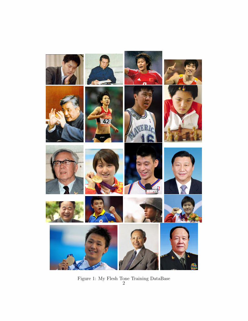
Figure 1: My Flesh Tone Training DataBase2
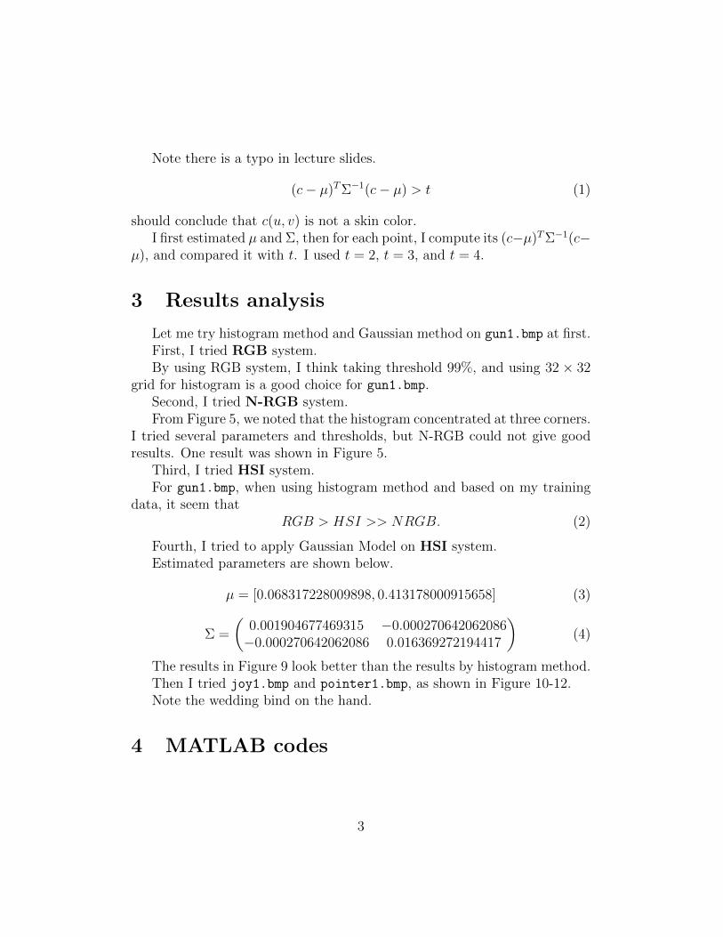
Note there is a typo in lecture slides.
(c− µ)TΣ−1(c− µ) > t (1)
should conclude that c(u, v) is not a skin color.I first estimated µ and Σ, then for each point, I compute its (c−µ)TΣ−1(c−
µ), and compared it with t. I used t = 2, t = 3, and t = 4.
3 Results analysis
Let me try histogram method and Gaussian method on gun1.bmp at first.First, I tried RGB system.By using RGB system, I think taking threshold 99%, and using 32 × 32
grid for histogram is a good choice for gun1.bmp.Second, I tried N-RGB system.From Figure 5, we noted that the histogram concentrated at three corners.
I tried several parameters and thresholds, but N-RGB could not give goodresults. One result was shown in Figure 5.
Third, I tried HSI system.For gun1.bmp, when using histogram method and based on my training
data, it seem thatRGB > HSI >> NRGB. (2)
Fourth, I tried to apply Gaussian Model on HSI system.Estimated parameters are shown below.
µ = [0.068317228009898, 0.413178000915658] (3)
Σ =
(0.001904677469315 −0.000270642062086−0.000270642062086 0.016369272194417
)(4)
The results in Figure 9 look better than the results by histogram method.Then I tried joy1.bmp and pointer1.bmp, as shown in Figure 10-12.Note the wedding bind on the hand.
4 MATLAB codes
3
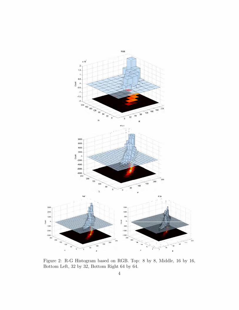
Figure 2: R-G Histogram based on RGB. Top: 8 by 8, Middle, 16 by 16,Bottom Left, 32 by 32, Bottom Right 64 by 64.
4
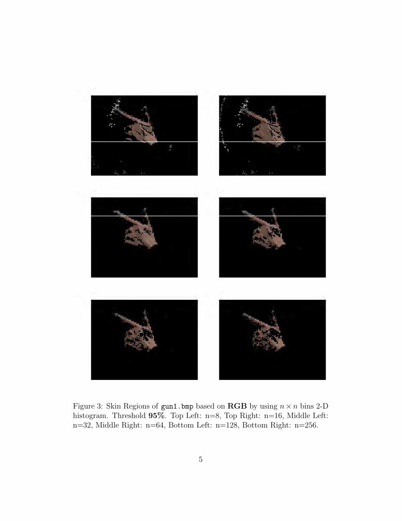
Figure 3: Skin Regions of gun1.bmp based on RGB by using n×n bins 2-Dhistogram. Threshold 95%. Top Left: n=8, Top Right: n=16, Middle Left:n=32, Middle Right: n=64, Bottom Left: n=128, Bottom Right: n=256.
5
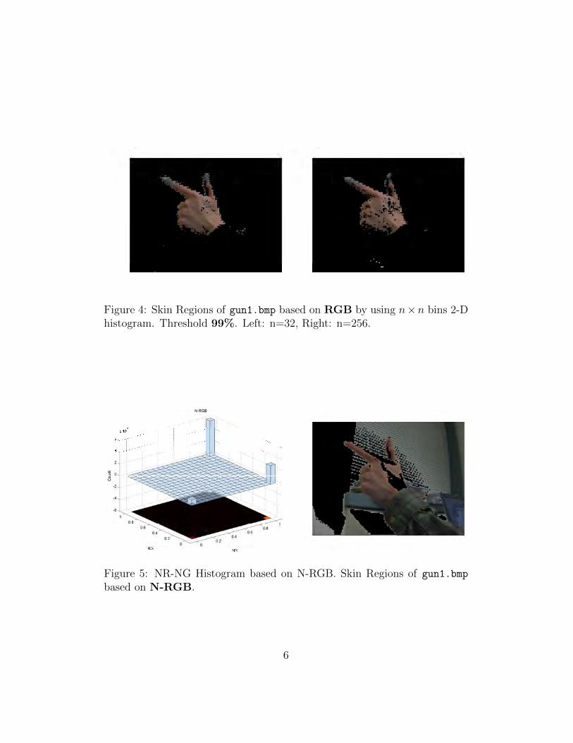
Figure 4: Skin Regions of gun1.bmp based on RGB by using n×n bins 2-Dhistogram. Threshold 99%. Left: n=32, Right: n=256.
Figure 5: NR-NG Histogram based on N-RGB. Skin Regions of gun1.bmp
based on N-RGB.
6
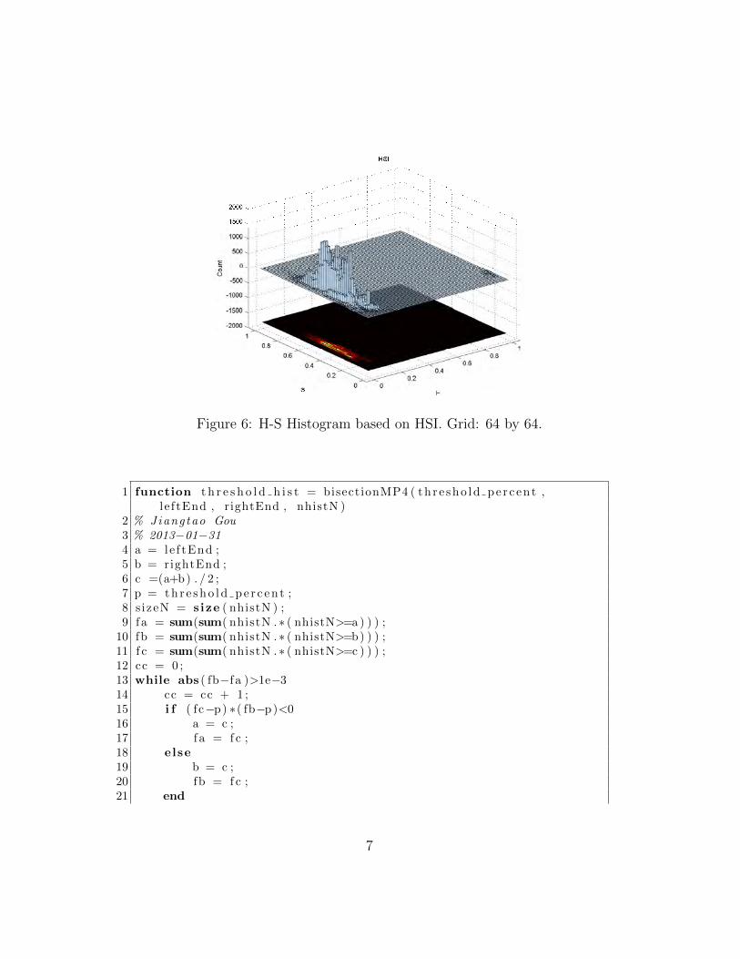
Figure 6: H-S Histogram based on HSI. Grid: 64 by 64.
1 function t h r e s h o l d h i s t = bisectionMP4 ( th r e sho ld pe r c en t ,le f tEnd , rightEnd , nhistN )
2 % Jiangtao Gou3 % 2013−01−314 a = le f tEnd ;5 b = rightEnd ;6 c =(a+b) . / 2 ;7 p = th r e sho l d pe r c en t ;8 s izeN = s ize ( nhistN ) ;9 f a = sum(sum( nhistN . ∗ ( nhistN>=a ) ) ) ;
10 fb = sum(sum( nhistN . ∗ ( nhistN>=b) ) ) ;11 f c = sum(sum( nhistN . ∗ ( nhistN>=c ) ) ) ;12 cc = 0 ;13 while abs ( fb−f a )>1e−314 cc = cc + 1 ;15 i f ( fc−p) ∗( fb−p)<016 a = c ;17 fa = f c ;18 else19 b = c ;20 fb = f c ;21 end
7
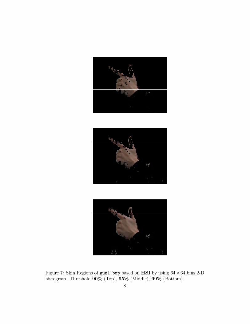
Figure 7: Skin Regions of gun1.bmp based on HSI by using 64×64 bins 2-Dhistogram. Threshold 90% (Top), 95% (Middle), 99% (Bottom).
8
00.2
0.40.6
0.81
0
0.2
0.4
0.6
0.8
10
5
10
15
20
25
H
HSI−Gaussian
S
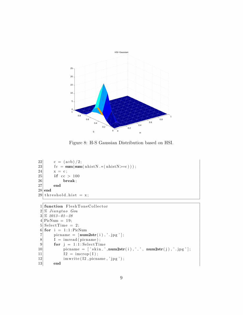
Figure 8: H-S Gaussian Distribution based on HSI.
22 c = ( a+b) /2 ;23 f c = sum(sum( nhistN . ∗ ( nhistN>=c ) ) ) ;24 x = c ;25 i f cc > 10026 break ;27 end28 end29 t h r e s h o l d h i s t = x ;
1 function FleshToneCol l ector2 % Jiangtao Gou3 % 2013−01−284 PicNum = 19 ;5 SelectTime = 2 ;6 for i = 1 : 1 : PicNum7 picname = [num2str( i ) , ’ . jpg ’ ] ;8 I = imread ( picname ) ;9 for j = 1 : 1 : SelectTime
10 picname = [ ’ s k i n ’ ,num2str( i ) , ’ ’ , num2str( j ) , ’ . jpg ’ ] ;11 I2 = imcrop ( I ) ;12 imwrite ( I2 , picname , ’ jpg ’ ) ;13 end
9
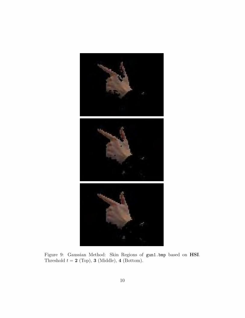
Figure 9: Gaussian Method: Skin Regions of gun1.bmp based on HSI.Threshold t = 2 (Top), 3 (Middle), 4 (Bottom).
10
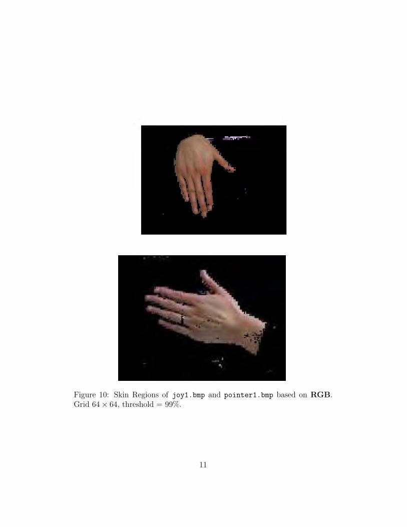
Figure 10: Skin Regions of joy1.bmp and pointer1.bmp based on RGB.Grid 64× 64, threshold = 99%.
11
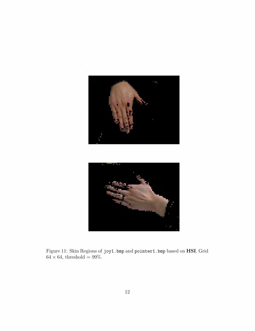
Figure 11: Skin Regions of joy1.bmp and pointer1.bmp based on HSI. Grid64× 64, threshold = 99%.
12

Figure 12: Gaussian Method: Skin Regions of joy1.bmp and pointer1.bmp
based on HSI. Threshold t = 4 .
13
14 end
1 function t h r e sho l d pe r c en t = ver i fyBisect ionMP4 ( th r e s ho l d h i s t ,nhistN )
2 % Jiangtao Gou3 % 2013−01−314 t = th r e s h o l d h i s t ;5 th r e sho l d pe r c en t = sum(sum( nhistN . ∗ ( nhistN>=t ) ) ) ;
1 function colorSpaceData = co lo rSpaceDataCo l l e c to r ( spaceType )2 % Jiangtao Gou3 % 2013−01−294 switch spaceType5 case 16 colorSpaceData = colorSpaceDataCollectorRGB ;7 case 28 colorSpaceData = colorSpaceDataCollectorNRGB ;9 case 3
10 colorSpaceData = co lorSpaceDataCol l ectorHSI ;11 otherwi se12 error ( ’Only RGB, nRGB, HSI are a v a i l a b l e temporar i ly . ’ )13 end
1 function colorSpaceData = colorSpaceDataCollectorRGB2 % Jiangtao Gou3 % 2013−01−304 PicNum = 19 ;5 SelectTime = 2 ;6 colorSpaceData = [ ] ;7 for i = 1 : 1 : PicNum8 for j = 1 : 1 : SelectTime9 picname = [ ’ s k i n ’ ,num2str( i ) , ’ ’ , num2str( j ) , ’ . jpg ’ ] ;
10 J = imread ( picname ) ;11 s i z e J = s ize ( J ) ;12 % A Faster way13 mat2D1 = J ( : , : , 1 ) ;14 mat2D2 = J ( : , : , 2 ) ;15 mat1D1 = reshape (mat2D1 , s i z e J (1 , 1 ) ∗ s i z e J (1 , 2 ) ,1 ) ;16 mat1D2 = reshape (mat2D2 , s i z e J (1 , 1 ) ∗ s i z e J (1 , 2 ) ,1 ) ;17 colorSpaceData = [ colorSpaceData ; [ mat1D1 ,mat1D2 ] ] ;18 % A Slower way19 % for k1 = 1 : 1 : s i z e J (1 ,1)20 % for k2 = 1 : 1 : s i z e J (1 ,2)21 % colorSpaceData = [ colorSpaceData ; [ J ( k1 , k2 , 1 ) ,
J ( k1 , k2 , 2 ) ] ] ;
14
22 % end23 % end24 end25 end26 colorSpaceData = double ( colorSpaceData ) ;27 %% Test28 % mat3D ( : , : , 1 ) = [ 1 , 3 , 5 , 6 ; 2 , 8 , 4 , 9 ] ;29 % mat3D ( : , : , 2 ) = [17 ,37 ,57 ,67 ;27 ,87 ,47 ,97 ] ;30 % mat2D1 = mat3D ( : , : , 1 ) ;31 % mat2D2 = mat3D ( : , : , 2 ) ;32 % mat1D1 = reshape (mat2D1 , prod ( s i z e (mat2D1) ) ,1) ;33 % mat1D2 = reshape (mat2D2 , prod ( s i z e (mat2D2) ) ,1) ;34 % mat1D = [mat1D1 ,mat1D2 ] ;
1 function colorSpaceData = colorSpaceDataCollectorNRGB2 % Jiangtao Gou3 % 2013−01−314 PicNum = 19 ;5 SelectTime = 2 ;6 colorSpaceData = [ ] ;7 for i = 1 : 1 : PicNum8 for j = 1 : 1 : SelectTime9 picname = [ ’ s k i n ’ ,num2str( i ) , ’ ’ , num2str( j ) , ’ . jpg ’ ] ;
10 J = imread ( picname ) ;11 s i z e J = s ize ( J ) ;12 mat2Dsum = J ( : , : , 1 )+J ( : , : , 2 )+J ( : , : , 3 ) ;13 mat2D1 = J ( : , : , 1 ) . /mat2Dsum ;14 mat2D2 = J ( : , : , 2 ) . /mat2Dsum ;15 mat1D1 = reshape (mat2D1 , s i z e J (1 , 1 ) ∗ s i z e J (1 , 2 ) ,1 ) ;16 mat1D2 = reshape (mat2D2 , s i z e J (1 , 1 ) ∗ s i z e J (1 , 2 ) ,1 ) ;17 colorSpaceData = [ colorSpaceData ; [ mat1D1 ,mat1D2 ] ] ;18 end19 end20 colorSpaceData = double ( colorSpaceData ) ;
1 function colorSpaceData = co lorSpaceDataCol l ectorHSI2 % Jiangtao Gou3 % 2013−01−314 PicNum = 19 ;5 SelectTime = 2 ;6 colorSpaceData = [ ] ;7 for i = 1 : 1 : PicNum8 for j = 1 : 1 : SelectTime9 picname = [ ’ s k i n ’ ,num2str( i ) , ’ ’ , num2str( j ) , ’ . jpg ’ ] ;
10 J = imread ( picname ) ;
15
11 rgb image = J ;12 hsv image = rgb2hsv ( rgb image ) ;13 J = hsv image ;14 s i z e J = s ize ( J ) ;15 mat2D1 = J ( : , : , 1 ) ;16 mat2D2 = J ( : , : , 2 ) ;17 mat1D1 = reshape (mat2D1 , s i z e J (1 , 1 ) ∗ s i z e J (1 , 2 ) ,1 ) ;18 mat1D2 = reshape (mat2D2 , s i z e J (1 , 1 ) ∗ s i z e J (1 , 2 ) ,1 ) ;19 colorSpaceData = [ colorSpaceData ; [ mat1D1 ,mat1D2 ] ] ;20 end21 end22 colorSpaceData = double ( colorSpaceData ) ;
1 function nh i s t = h i s tP l o t 1 ( colorSpaceData , nBins )2 % From MATLAB ” h i s t 3 ” B i va r i a t e his togram3 % Jiangtao Gou4 % 2013−01−315 dat = colorSpaceData ;6 kk = 256/ nBins ;7 %h i s t 3 ( dat , [ nBins nBins ] , ’ FaceAlpha ’ , . 6 5 ) ; % Draw histogram in 2
D8 h i s t 3 ( dat , { 0 : kk :255 0 : kk :255} , ’ FaceAlpha ’ , . 6 5 ) ;9 hold on ;
10 xlabel ( ’R ’ ) ;11 ylabel ( ’G’ ) ;12 %n = h i s t 3 ( dat , [ nBins nBins ] , ’ FaceAlpha ’ , . 6 5 ) ; % Extrac t
his togram data ;13 n= h i s t 3 ( dat , { 0 : kk :255 0 : kk :255} , ’ FaceAlpha ’ , . 6 5 ) ;14 n1 = n ’ ;15 n1 ( s ize (n , 1 ) + 1 , s ize (n , 2 ) + 1 ) = 0 ;16 % Generate g r i d f o r 2−D pro j e c t e d view o f i n t e n s i t i e s17 xb = linspace (min( dat ( : , 1 ) ) ,max( dat ( : , 1 ) ) , s ize (n , 1 ) +1) ;18 yb = linspace (min( dat ( : , 2 ) ) ,max( dat ( : , 2 ) ) , s ize (n , 1 ) +1) ;19 % Make a pseudoco lor p l o t on t h i s g r i d20 h = pcolor (xb , yb , n1 ) ;21 % Set the z− l e v e l and colormap o f the d i s p l a y ed g r i d22 set (h , ’ zdata ’ , ones ( s ize ( n1 ) ) ∗ −max(max(n) ) )23 colormap (hot ) % heat map24 t i t l e ( ’RGB’ ) ;25 zlabel ( ’Count ’ ) ;26 set ( gcf , ’ r ende re r ’ , ’ opengl ’ ) ;27 grid on28 % Disp lay the d e f a u l t 3−D pe r s p e c t i v e view29 view (3 ) ;30 hold o f f ;
16
31 nh i s t = n ;32 %%33 set ( gcf , ’ p ape r s i z e ’ , [ 5 8 ] ) ;34 picname = [ ’ h i s t . eps ’ ] ;35 saveas ( gcf , picname , ’ epsc ’ ) ;36 eps2pdf ( picname ) ;
1 function nh i s t = h i s tP l o t 2 ( colorSpaceData , nBins )2 % Jiangtao Gou3 % 2013−01−314 dat = colorSpaceData ;5 kk = 1/nBins ;6 %h i s t 3 ( dat , [ nBins nBins ] , ’ FaceAlpha ’ , . 6 5 ) ; % Draw histogram in 2
D7 h i s t 3 ( dat , { 0 : kk : 1 0 : kk : 1} , ’ FaceAlpha ’ , . 6 5 ) ;8 hold on ;9 xlabel ( ’NR’ ) ;
10 ylabel ( ’NG’ ) ;11 %n = h i s t 3 ( dat , [ nBins nBins ] , ’ FaceAlpha ’ , . 6 5 ) ; % Extrac t
his togram data ;12 n= h i s t 3 ( dat , { 0 : kk : 1 0 : kk : 1} , ’ FaceAlpha ’ , . 6 5 ) ;13 n1 = n ’ ;14 n1 ( s ize (n , 1 ) + 1 , s ize (n , 2 ) + 1 ) = 0 ;15 % Generate g r i d f o r 2−D pro j e c t e d view o f i n t e n s i t i e s16 xb = linspace (min( dat ( : , 1 ) ) ,max( dat ( : , 1 ) ) , s ize (n , 1 ) +1) ;17 yb = linspace (min( dat ( : , 2 ) ) ,max( dat ( : , 2 ) ) , s ize (n , 1 ) +1) ;18 % Make a pseudoco lor p l o t on t h i s g r i d19 h = pcolor (xb , yb , n1 ) ;20 % Set the z− l e v e l and colormap o f the d i s p l a y ed g r i d21 set (h , ’ zdata ’ , ones ( s ize ( n1 ) ) ∗ −max(max(n) ) )22 colormap (hot ) % heat map23 t i t l e ( ’N−RGB’ ) ;24 zlabel ( ’Count ’ ) ;25 set ( gcf , ’ r ende re r ’ , ’ opengl ’ ) ;26 grid on27 % Disp lay the d e f a u l t 3−D pe r s p e c t i v e view28 view (3 ) ;29 hold o f f ;30 nh i s t = n ;31 %%32 set ( gcf , ’ p ape r s i z e ’ , [ 5 8 ] ) ;33 picname = [ ’ h i s t n . eps ’ ] ;34 saveas ( gcf , picname , ’ epsc ’ ) ;35 eps2pdf ( picname ) ;
17
1 function nh i s t = h i s tP l o t 3 ( colorSpaceData , nBins )2 % Jiangtao Gou3 % 2013−01−314 dat = colorSpaceData ;5 minH = min( dat ( : , 1 ) ) ;6 maxH = max( dat ( : , 1 ) ) ;7 minS = min( dat ( : , 2 ) ) ;8 maxS = max( dat ( : , 2 ) ) ;9 kH = (maxH−minH) /nBins ;
10 kS = (maxS−minS) /nBins ;11 %h i s t 3 ( dat , [ nBins nBins ] , ’ FaceAlpha ’ , . 6 5 ) ; % Draw histogram in 2
D12 h i s t 3 ( dat ,{minH :kH:maxH minS : kS :maxS} , ’ FaceAlpha ’ , . 6 5 ) ;13 hold on ;14 xlabel ( ’H ’ ) ;15 ylabel ( ’S ’ ) ;16 %n = h i s t 3 ( dat , [ nBins nBins ] , ’ FaceAlpha ’ , . 6 5 ) ; % Extrac t
his togram data ;17 n= h i s t 3 ( dat ,{minH :kH:maxH minS : kS :maxS} , ’ FaceAlpha ’ , . 6 5 ) ;18 n1 = n ’ ;19 n1 ( s ize (n , 1 ) + 1 , s ize (n , 2 ) + 1 ) = 0 ;20 % Generate g r i d f o r 2−D pro j e c t e d view o f i n t e n s i t i e s21 xb = linspace (min( dat ( : , 1 ) ) ,max( dat ( : , 1 ) ) , s ize (n , 1 ) +1) ;22 yb = linspace (min( dat ( : , 2 ) ) ,max( dat ( : , 2 ) ) , s ize (n , 1 ) +1) ;23 % Make a pseudoco lor p l o t on t h i s g r i d24 h = pcolor (xb , yb , n1 ) ;25 % Set the z− l e v e l and colormap o f the d i s p l a y ed g r i d26 set (h , ’ zdata ’ , ones ( s ize ( n1 ) ) ∗ −max(max(n) ) )27 colormap (hot ) % heat map28 t i t l e ( ’HSI ’ ) ;29 zlabel ( ’Count ’ ) ;30 set ( gcf , ’ r ende re r ’ , ’ opengl ’ ) ;31 grid on32 % Disp lay the d e f a u l t 3−D pe r s p e c t i v e view33 view (3 ) ;34 hold o f f ;35 nh i s t = n ;36 %%37 set ( gcf , ’ p ape r s i z e ’ , [ 5 8 ] ) ;38 picname = [ ’ h i s t h s . eps ’ ] ;39 saveas ( gcf , picname , ’ epsc ’ ) ;40 eps2pdf ( picname ) ;
1 function [ r e su l tP i c , r e s u l tP i cCo l o r ] = skinRegionSearcherRGB (
18
picname , sgnHist , nBins )2 % Jiangtao Gou3 % 2013−01−314 k = 256/ nBins ;5 sgnRGB = kron ( sgnHist , ones (k , k ) ) ;6 % picname = ’ gun1 . bmp ’ ;7 SK = imread ( picname ) ;8 r e su l tP i cCo l o r = SK;9 sizeSK = s ize (SK) ;
10 r e s u l tP i c = zeros ( s izeSK (1 , 1 ) , s izeSK (1 , 2 ) ) ;11 for i = 1 : 1 : s izeSK (1 , 1 )12 for j = 1 : 1 : s izeSK (1 , 2 )13 i f sgnRGB(SK( i , j , 1 ) +1,SK( i , j , 2 ) +1) == 114 r e s u l tP i c ( i , j ) = 1 ;15 else16 r e s u l tP i c ( i , j ) = 0 ;17 r e su l tP i cCo l o r ( i , j , 1 ) = 0 ;18 r e su l tP i cCo l o r ( i , j , 2 ) = 0 ;19 r e su l tP i cCo l o r ( i , j , 3 ) = 0 ;20 end21 end22 end
1 function [ r e su l tP i c , r e s u l tP i cCo l o r ] = skinRegionSearcherNrgb (picname , sgnHist , nBins )
2 % Jiangtao Gou3 % 2013−01−314 k = 1/nBins ;5 % picname = ’ gun1 . bmp ’ ;6 SK = imread ( picname ) ;7 SKsum = SK( : , : , 1 )+SK( : , : , 2 )+SK( : , : , 3 ) ;8 SKN1 = SK( : , : , 1 ) . /SKsum;9 SKN2 = SK( : , : , 2 ) . /SKsum;
10 r e su l tP i cCo l o r = SK;11 sizeSK = s ize (SK) ;12 r e s u l tP i c = zeros ( s izeSK (1 , 1 ) , s izeSK (1 , 2 ) ) ;13 for i = 1 : 1 : s izeSK (1 , 1 )14 for j = 1 : 1 : s izeSK (1 , 2 )15 xx = ce i l (SKN1( i , j ) /k ) ;16 yy = ce i l (SKN2( i , j ) /k ) ;17 i f xx == 018 xx = 1 ;19 end20 i f yy == 021 yy = 1 ;
19
22 end23 i f sgnHist ( xx , yy ) == 124 r e s u l tP i c ( i , j ) = 1 ;25 else26 r e s u l tP i c ( i , j ) = 0 ;27 r e su l tP i cCo l o r ( i , j , 1 ) = 0 ;28 r e su l tP i cCo l o r ( i , j , 2 ) = 0 ;29 r e su l tP i cCo l o r ( i , j , 3 ) = 0 ;30 end31 end32 end
1 function [ r e su l tP i c , r e s u l tP i cCo l o r ] = skinRegionSearcherHSI (picname , sgnHist , nBins , colorSpaceData )
2 % Jiangtao Gou3 % 2013−01−314 dat = colorSpaceData ;5 minH = min( dat ( : , 1 ) ) ;6 maxH = max( dat ( : , 1 ) ) ;7 minS = min( dat ( : , 2 ) ) ;8 maxS = max( dat ( : , 2 ) ) ;9 kH = (maxH−minH) /nBins ;
10 kS = (maxS−minS) /nBins ;11 % picname = ’ gun1 . bmp ’ ;12 SK = imread ( picname ) ;13 rgb image = SK;14 hsv image = rgb2hsv ( rgb image ) ;15 SK = hsv image ;16 r e su l tP i cCo l o r = SK;17 sizeSK = s ize (SK) ;18 r e s u l tP i c = zeros ( s izeSK (1 , 1 ) , s izeSK (1 , 2 ) ) ;19 for i = 1 : 1 : s izeSK (1 , 1 )20 for j = 1 : 1 : s izeSK (1 , 2 )21 hh = ce i l ( (SK( i , j , 1 )−minH) /kH) ;22 s s = ce i l ( (SK( i , j , 2 )−minS) /kS ) ;23 i f (SK( i , j , 1 ) >= maxH) | | ( SK( i , j , 1 ) <= minH) | | ( SK( i , j , 2 )
>= maxS) | | ( SK( i , j , 2 ) <= minS)24 r e s u l tP i c ( i , j ) = 0 ;25 r e su l tP i cCo l o r ( i , j , 1 ) = 0 ;26 r e su l tP i cCo l o r ( i , j , 2 ) = 0 ;27 r e su l tP i cCo l o r ( i , j , 3 ) = 0 ;28 e l s e i f sgnHist (hh , s s ) == 029 r e s u l tP i c ( i , j ) = 0 ;30 r e su l tP i cCo l o r ( i , j , 1 ) = 0 ;31 r e su l tP i cCo l o r ( i , j , 2 ) = 0 ;
20
32 r e su l tP i cCo l o r ( i , j , 3 ) = 0 ;33 else34 r e s u l tP i c ( i , j ) = 1 ;35 end36 end37 end38 r e su l tP i cCo l o r = hsv2rgb ( r e su l tP i cCo l o r ) ;
1 function r e su l tP i cCo l o r = skinRegionSearcherGauss ian ( picname ,mu,sigma , colorSpaceData , c )
2 % For HSI only3 % Jiangtao Gou4 % 2013−01−315 SK = imread ( picname ) ;6 rgb image = SK;7 hsv image = rgb2hsv ( rgb image ) ;8 SK = hsv image ;9 r e su l tP i cCo l o r = SK;
10 sizeSK = s ize (SK) ;11 for i = 1 : 1 : s izeSK (1 , 1 )12 for j = 1 : 1 : s izeSK (1 , 2 )13 vec = [SK( i , j , 1 ) ; SK( i , j , 2 ) ] − mu’ ;14 normDev = vec ’∗ inv ( sigma ) ∗vec ;15 i f normDev > c16 r e su l tP i cCo l o r ( i , j , 1 ) = 0 ;17 r e su l tP i cCo l o r ( i , j , 2 ) = 0 ;18 r e su l tP i cCo l o r ( i , j , 3 ) = 0 ;19 end20 end21 end22 r e su l tP i cCo l o r = hsv2rgb ( r e su l tP i cCo l o r ) ;
1 function MP4 main2 % Jiangtao Gou3 % 2013−01−314 FleshToneCol l ec tor ;5 % 1−RGB, 2−nRGB, 3−HSI6 colorSpaceData = co lo rSpaceDataCo l l e c to r (1 ) ;7 nBins = 64 ;8 nh i s t = h i s tP l o t 1 ( colorSpaceData , nBins ) ;9 nhistN = 1/sum(sum( nh i s t ) ) ∗ nh i s t ;
10 l e f tEnd = min(min( nhistN ) ) ;11 rightEnd = max(max( nhistN ) ) /4 ;12 th r e sho l d pe r c en t = 0 . 9 9 ;
21
13 t h r e s h o l d h i s t = bisectionMP4 ( th r e sho ld pe r c en t , le f tEnd ,rightEnd , nhistN ) ;
14 %15 th r e sho l d pe r c en t = ver i fyBisect ionMP4 ( th r e s ho l d h i s t , nhistN ) ;16 %17 sgnHist = ( nhistN >= th r e s h o l d h i s t ) ;18 %19 picname1 = ’ po in t e r1 .bmp ’ ;20 f i l ename1 = ’ po in te r1 ’ ;21 [ r e su l tP i c , r e su l tP i cCo l o r ] = skinRegionSearcherRGB ( picname1 ,
sgnHist , nBins ) ;22 %imshow( r e su l tP i c , [ 0 , 1 ] ) ;23 imshow( r e su l tP i cCo l o r ) ;24 f i l ename = f i l ename1 ;25 set ( gcf , ’ p ape r s i z e ’ , [ 5 6 ] ) ;26 picname = [ f i l ename , ’ . eps ’ ] ;27 saveas ( gcf , picname , ’ epsc ’ ) ;28 eps2pdf ( picname ) ;
1 function MP4 main 22 % Jiangtao Gou3 % 2013−01−314 % 1−RGB, 2−nRGB, 3−HSI5 colorSpaceData = co lo rSpaceDataCo l l e c to r (2 ) ;6 nBins = 16 ;7 nh i s t = h i s tP l o t 2 ( colorSpaceData , nBins ) ;8 nhistN = 1/sum(sum( nh i s t ) ) ∗ nh i s t ;9 l e f tEnd = min(min( nhistN ) ) ;
10 rightEnd = max(max( nhistN ) ) ;11 th r e sho l d pe r c en t = 0 . 9 2 ;12 t h r e s h o l d h i s t = bisectionMP4 ( th r e sho ld pe r c en t , le f tEnd ,
rightEnd , nhistN ) ;13 %14 th r e sho l d pe r c en t = ver i fyBisect ionMP4 ( th r e s ho l d h i s t , nhistN ) ;15 %16 sgnHist = ( nhistN >= th r e s h o l d h i s t ) ;17 %18 picname1 = ’ gun1 .bmp ’ ;19 f i l ename1 = ’ gun1 n ’ ;20 [ r e su l tP i c , r e su l tP i cCo l o r ] = skinRegionSearcherNrgb ( picname1 ,
sgnHist , nBins ) ;21 %imshow( r e su l tP i c , [ 0 , 1 ] ) ;22 imshow( r e su l tP i cCo l o r ) ;23 f i l ename = f i l ename1 ;24 set ( gcf , ’ p ape r s i z e ’ , [ 5 6 ] ) ;
22
25 picname = [ f i l ename , ’ . eps ’ ] ;26 saveas ( gcf , picname , ’ epsc ’ ) ;27 eps2pdf ( picname ) ;
1 function MP4 main 32 % Jiangtao Gou3 % 2013−01−314 % 1−RGB, 2−nRGB, 3−HSI5 colorSpaceData = co lo rSpaceDataCo l l e c to r (3 ) ;6 nBins = 64 ;7 nh i s t = h i s tP l o t 3 ( colorSpaceData , nBins ) ;8 %9 nhistN = 1/sum(sum( nh i s t ) ) ∗ nh i s t ;
10 l e f tEnd = min(min( nhistN ) ) ;11 rightEnd = max(max( nhistN ) ) ;12 th r e sho l d pe r c en t = 0 . 9 9 ;13 t h r e s h o l d h i s t = bisectionMP4 ( th r e sho ld pe r c en t , le f tEnd ,
rightEnd , nhistN ) ;14 %15 th r e sho l d pe r c en t = ver i fyBisect ionMP4 ( th r e s ho l d h i s t , nhistN ) ;16 %17 sgnHist = ( nhistN >= th r e s h o l d h i s t ) ;18 %19 picname1 = ’ joy1 .bmp ’ ;20 f i l ename1 = ’ joy1 hs ’ ;21 [ r e su l tP i c , r e su l tP i cCo l o r ] = skinRegionSearcherHSI ( picname1 ,
sgnHist , nBins , colorSpaceData ) ;22 %imshow( r e su l tP i c , [ 0 , 1 ] ) ;23 imshow( r e su l tP i cCo l o r ) ;24 f i l ename = f i l ename1 ;25 set ( gcf , ’ p ape r s i z e ’ , [ 5 6 ] ) ;26 picname = [ f i l ename , ’ . eps ’ ] ;27 saveas ( gcf , picname , ’ epsc ’ ) ;28 eps2pdf ( picname ) ;
1 function MP4 main Gaussian2 % For HSI only3 % Jiangtao Gou4 % 2013−01−315 colorSpaceData = colorSpaceDataCol l ectorHSI ;6 mu = mean( colorSpaceData ) ;7 sigma = cov ( colorSpaceData ) ;8 %9 c = 4 ;
10 picname1 = ’ po in t e r1 .bmp ’ ;
23
11 f i l ename1 = ’ po in t e r 1 gau s s i an ’ ;12 r e su l tP i cCo l o r = skinRegionSearcherGauss ian ( picname1 ,mu, sigma ,
colorSpaceData , c ) ;13 imshow( r e su l tP i cCo l o r ) ;14 f i l ename = f i l ename1 ;15 set ( gcf , ’ p ape r s i z e ’ , [ 5 6 ] ) ;16 picname = [ f i l ename , ’ . eps ’ ] ;17 saveas ( gcf , picname , ’ epsc ’ ) ;18 eps2pdf ( picname ) ;19 %20 minHS = min( colorSpaceData ) ;21 maxHS = max( colorSpaceData ) ;22 x = minHS(1) : ( (maxHS(1)−minHS(1) ) /10) :maxHS(1) ;23 y = minHS(2) : ( (maxHS(2)−minHS(2) ) /10) :maxHS(2) ;24 [X,Y]=meshgrid (x , y ) ;25 p=mvnpdf ( [X( : ) ,Y( : ) ] ,mu, sigma ) ;26 P=reshape (p , s ize (X) ) ;27 surf (X,Y,P)28 shading f l a t29 xlabel ( ’H ’ ) ;30 ylabel ( ’S ’ ) ;31 t i t l e ( ’HSI−Gaussian ’ ) ;32 set ( gcf , ’ p ape r s i z e ’ , [ 5 8 ] ) ;33 picname = [ ’ gaus s i an hs . eps ’ ] ;34 saveas ( gcf , picname , ’ epsc ’ ) ;35 eps2pdf ( picname ) ;36 %
24
Winter 2013 EECS 332 Digital Image Analysis
Machine Problem 5Canny Edge Detector
Jiangtao GouDepartment of Statistics, Northwestern University
Instructor: Prof. Ying Wu
26 February 2013
1 Introduction
In this report, I implemented the Canny edge detector by using MATLAB.
2 Algorithm Description
The first step is to use Gaussian smoothing as a filter to get rid of imagenoise by using Gaussian kernel.
When the picture is relatively smooth, I compute the image gradient bySobel operators, which used 3 by 3 grid to compute, and should give betterresults than Robert Cross operators, which used 2 by 2 grid.
Then I choose high and low thresholds. As Professor suggested, I choosehigh threshold to achieve 80% above, and choose low threshold as half ofhigh threshold.
The fourth step is to supress non-maxima. In the following I linked theedges by using the recursive algorithm, where I randomly choose the startpoint, and link edges.
Parameter N and σ were changed to see the different effects.
3 Results analysis
Some computation could be slow. The results are shown in those picturesbelow.
1
I tested my edge detector on all four pictures which provided by professor.Meanwhile, I use the whole body picture of Lena as the case of my own totest this edge detector.
The results are presented in these pictures.
4 MATLAB codes
1 function E=EdgeLinking (Mag low , Mag high )23 [ row , c o l ]= find (Mag high>0) ;4 for t =1:1 : s ize ( c o l )5 i f ( row ( t )<s ize ( c o l ) & co l ( t )<s ize ( c o l ) )6 i f (Mag low ( row ( t )+1, c o l ( t ) )>0)7 Mag high ( row ( t )+1, c o l ( t ) )=1;8 Mag low ( row ( t )+1, c o l ( t ) )=0;9 end
10 i f (Mag low ( row ( t ) , c o l ( t )+1)>0)11 Mag high ( row ( t ) , c o l ( t )+1)=1;12 Mag low ( row ( t ) , c o l ( t )+1)=0;13 end14 i f (Mag low ( row ( t )+1, c o l ( t )+1)>0)15 Mag high ( row ( t )+1, c o l ( t )+1)=1;16 Mag low ( row ( t )+1, c o l ( t )+1)=0;17 end18 i f (Mag low ( row ( t )−1, c o l ( t )−1)>0)19 Mag high ( row ( t )−1, c o l ( t )−1)=1;20 Mag low ( row ( t )−1, c o l ( t )−1)=0;21 end22 i f (Mag low ( row ( t )+1, c o l ( t )−1)>0)23 Mag high ( row ( t )+1, c o l ( t )−1)=1;24 Mag low ( row ( t )+1, c o l ( t )−1)=0;25 end26 i f (Mag low ( row ( t )−1, c o l ( t )+1)>0)27 Mag high ( row ( t )−1, c o l ( t )+1)=1;28 Mag low ( row ( t )−1, c o l ( t )+1)=0;29 end30 i f (Mag low ( row ( t )−1, c o l ( t ) )>0)31 Mag high ( row ( t )−1, c o l ( t ) )=1;32 Mag low ( row ( t )−1, c o l ( t ) )=0;33 end34 i f (Mag low ( row ( t ) , c o l ( t )−1)>0)35 Mag high ( row ( t ) , c o l ( t )−1)=1;36 Mag low ( row ( t ) , c o l ( t )−1)=0;
2
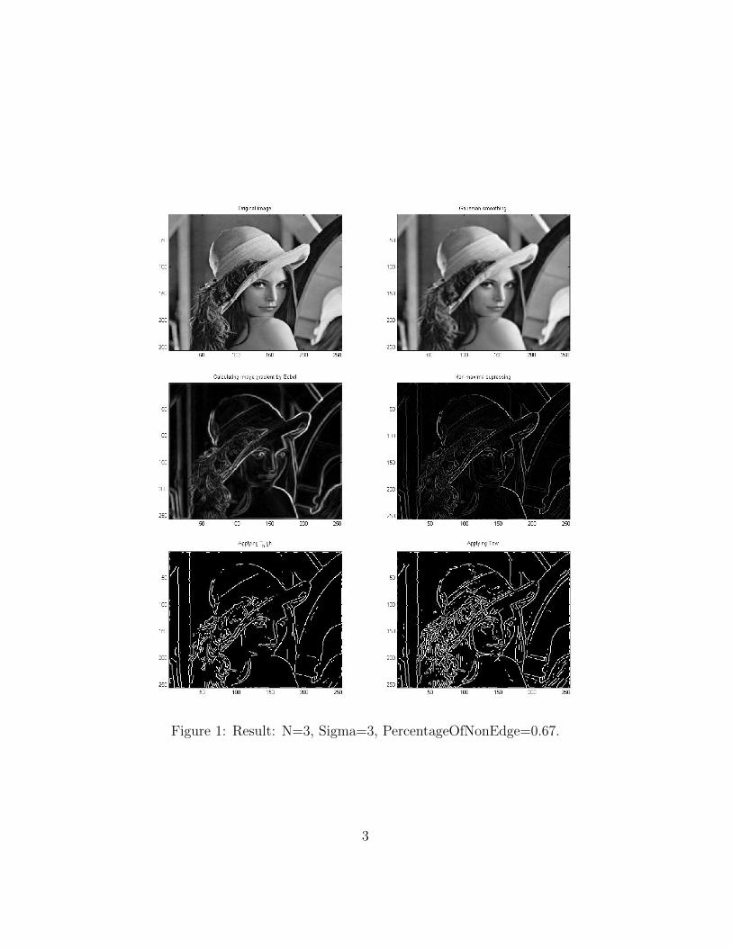
Figure 1: Result: N=3, Sigma=3, PercentageOfNonEdge=0.67.
3
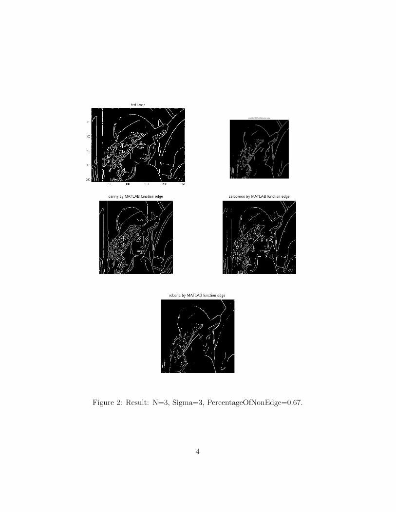
Figure 2: Result: N=3, Sigma=3, PercentageOfNonEdge=0.67.
4
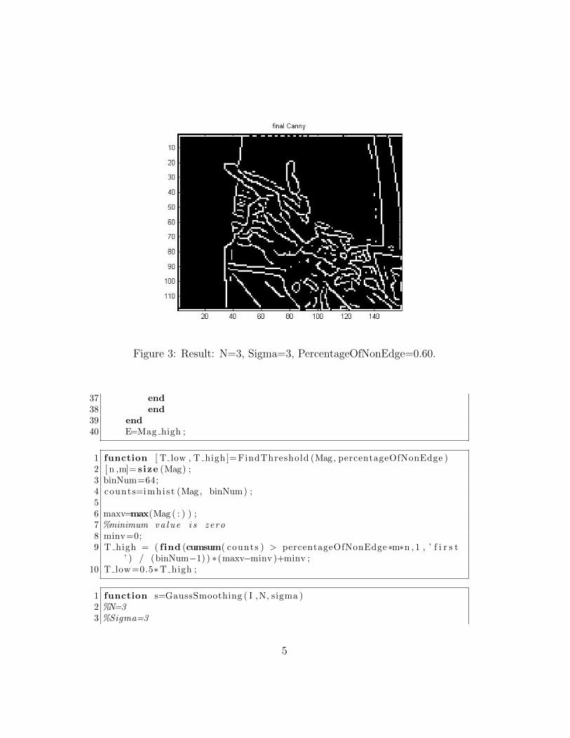
Figure 3: Result: N=3, Sigma=3, PercentageOfNonEdge=0.60.
37 end38 end39 end40 E=Mag high ;
1 function [ T low , T high ]=FindThreshold (Mag, percentageOfNonEdge )2 [ n ,m]= s ize (Mag) ;3 binNum=64;4 counts=imhis t (Mag, binNum) ;56 maxv=max(Mag ( : ) ) ;7 %minimum va lue i s zero8 minv=0;9 T high = ( find (cumsum( counts ) > percentageOfNonEdge∗m∗n , 1 , ’ f i r s t
’ ) / (binNum−1) ) ∗(maxv−minv )+minv ;10 T low=0.5∗T high ;
1 function s=GaussSmoothing ( I ,N, sigma )2 %N=33 %Sigma=3
5
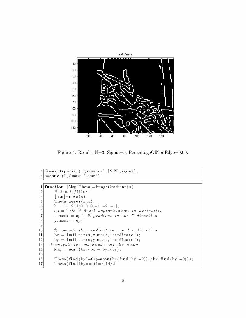
Figure 4: Result: N=3, Sigma=5, PercentageOfNonEdge=0.60.
4 Gmask=f s p e c i a l ( ’ gauss ian ’ , [N,N] , sigma ) ;5 s=conv2 ( I ,Gmask , ’ same ’ ) ;
1 function [Mag, Theta ]=ImageGradient ( s )2 % Sobe l f i l t e r3 [ n ,m]= s ize ( s ) ;4 Theta=zeros (n ,m) ;5 h = [1 2 1 ;0 0 0;−1 −2 −1];6 op = h/8 ; % Sobe l approximation to d e r i v a t i v e7 x mask = op ’ ; % grad i en t in the X d i r e c t i o n8 y mask = op ;9
10 % compute the g rad i en t in x and y d i r e c t i o n11 bx = im f i l t e r ( s , x mask , ’ r e p l i c a t e ’ ) ;12 by = im f i l t e r ( s , y mask , ’ r e p l i c a t e ’ ) ;13 % compute the magnitude and d i r e c t i o n14 Mag = sqrt ( bx .∗ bx + by .∗ by ) ;1516 Theta ( find ( by˜=0) )=atan ( bx ( find ( by˜=0) ) . / by ( find ( by˜=0) ) ) ;17 Theta ( find ( by==0)) =3.14/2;
6
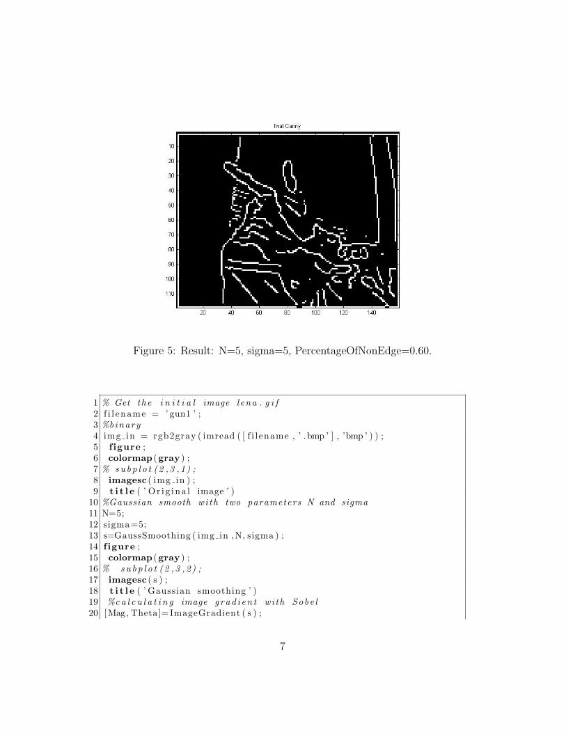
Figure 5: Result: N=5, sigma=5, PercentageOfNonEdge=0.60.
1 % Get the i n i t i a l image lena . g i f2 f i l ename = ’ gun1 ’ ;3 %binary4 img in = rgb2gray ( imread ( [ f i l ename , ’ .bmp ’ ] , ’bmp ’ ) ) ;5 f igure ;6 colormap (gray ) ;7 % subp l o t (2 ,3 ,1) ;8 imagesc ( img in ) ;9 t i t l e ( ’ Or i g ina l image ’ )
10 %Gaussian smooth wi th two parameters N and sigma11 N=5;12 sigma=5;13 s=GaussSmoothing ( img in ,N, sigma ) ;14 f igure ;15 colormap (gray ) ;16 % subp l o t (2 ,3 ,2) ;17 imagesc ( s ) ;18 t i t l e ( ’ Gaussian smoothing ’ )19 %ca l c u l a t i n g image g rad i en t wi th Sobe l20 [Mag, Theta ]=ImageGradient ( s ) ;
7
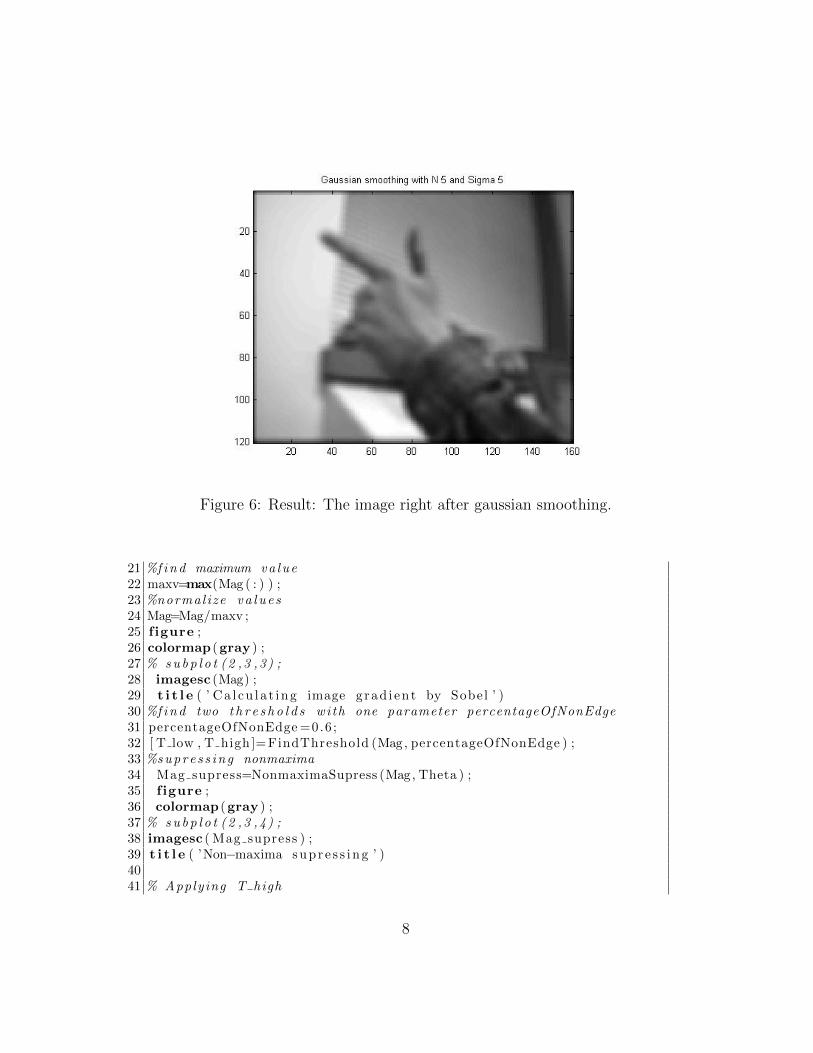
Figure 6: Result: The image right after gaussian smoothing.
21 %f ind maximum va lue22 maxv=max(Mag ( : ) ) ;23 %normal ize va l u e s24 Mag=Mag/maxv ;25 f igure ;26 colormap (gray ) ;27 % subp l o t (2 ,3 ,3) ;28 imagesc (Mag) ;29 t i t l e ( ’ Ca l cu l a t ing image grad i en t by Sobel ’ )30 %f ind two t h r e s h o l d s wi th one parameter percentageOfNonEdge31 percentageOfNonEdge =0.6 ;32 [ T low , T high ]=FindThreshold (Mag, percentageOfNonEdge ) ;33 %supre s s ing nonmaxima34 Mag supress=NonmaximaSupress (Mag, Theta ) ;35 f igure ;36 colormap (gray ) ;37 % subp l o t (2 ,3 ,4) ;38 imagesc ( Mag supress ) ;39 t i t l e ( ’Non−maxima supr e s s i ng ’ )4041 % Applying T high
8
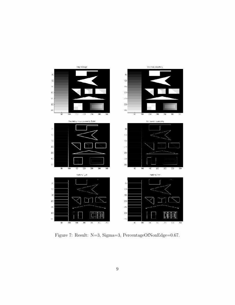
Figure 7: Result: N=3, Sigma=3, PercentageOfNonEdge=0.67.
9
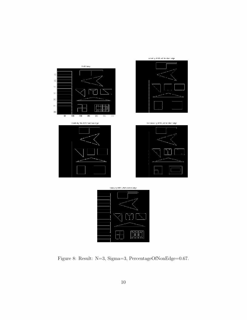
Figure 8: Result: N=3, Sigma=3, PercentageOfNonEdge=0.67.
10
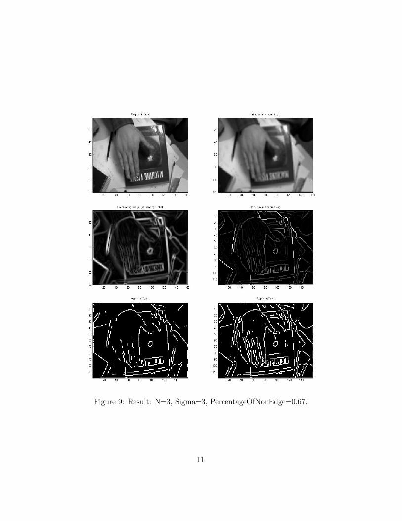
Figure 9: Result: N=3, Sigma=3, PercentageOfNonEdge=0.67.
11
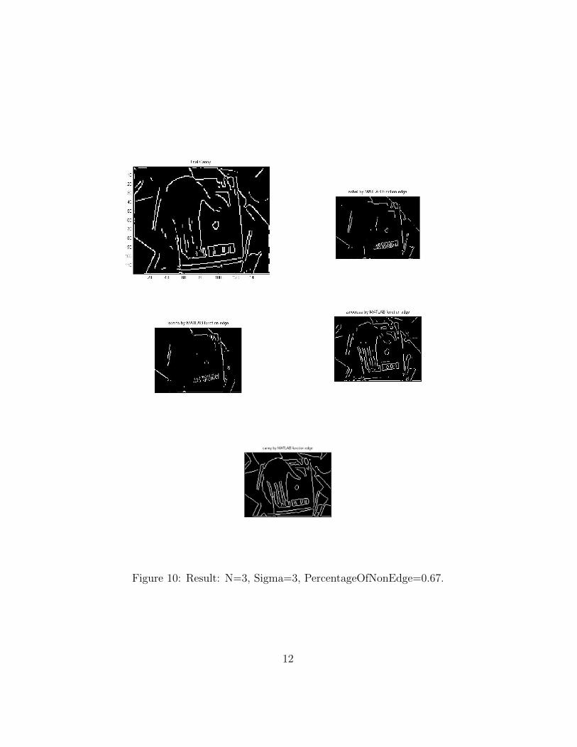
Figure 10: Result: N=3, Sigma=3, PercentageOfNonEdge=0.67.
12
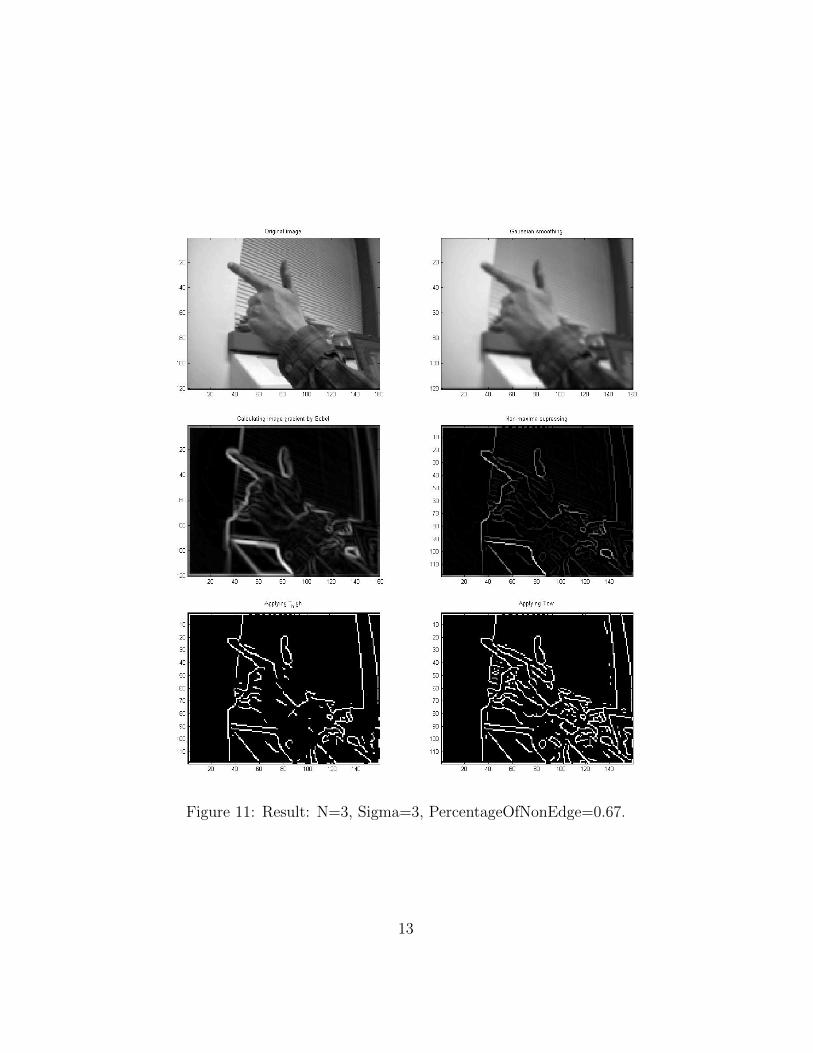
Figure 11: Result: N=3, Sigma=3, PercentageOfNonEdge=0.67.
13

Figure 12: Result: N=3, Sigma=3, PercentageOfNonEdge=0.67.
14
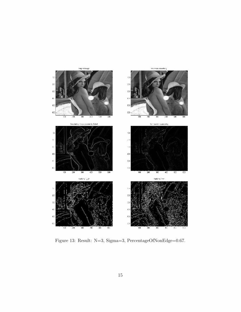
Figure 13: Result: N=3, Sigma=3, PercentageOfNonEdge=0.67.
15
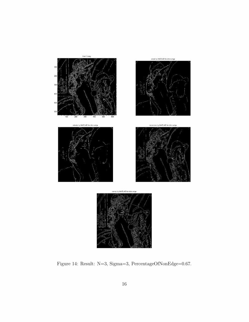
Figure 14: Result: N=3, Sigma=3, PercentageOfNonEdge=0.67.
16
42 Mag high=Mag supress ;43 Mag high ( find ( Mag supress<T high ) )=0;44 Mag high ( find ( Mag supress>=T high ) )=1;45 f igure ;46 colormap (gray )47 % subp l o t (2 ,3 ,5) ;48 imagesc (Mag high ) ;49 t i t l e ( ’ Applying T high ’ ) ;5051 % Applying T low52 Mag low=Mag supress ;53 Mag low ( find ( Mag supress<T low ) )=0;54 Mag low ( find ( Mag supress>=T low ) )=1;55 f igure ;56 colormap (gray )57 % subp l o t (2 ,3 ,6) ;58 imagesc (Mag low )59 t i t l e ( ’ Applying T low ’ ) ;60 %Edge l i n k i n g61 E=EdgeLinking (Mag low , Mag high ) ;62 f igure63 colormap (gray )64 imagesc (E) ;65 t i t l e ( ’ f i n a l Canny ’ ) ;6667 f igure68 edge ( img in , ’ s obe l ’ )69 t i t l e ( ’ s obe l by MATLAB func t i on edge ’ )70 f igure71 edge ( img in , ’ r ob e r t s ’ )72 t i t l e ( ’ r ob e r t s by MATLAB func t i on edge ’ )73 f igure74 edge ( img in , ’ z e r o c r o s s ’ )75 t i t l e ( ’ z e r o c r o s s by MATLAB func t i on edge ’ )76 f igure77 edge ( img in , ’ canny ’ )78 t i t l e ( ’ canny by MATLAB func t i on edge ’ )7980 t t =1;
1 function Mag supress=NonmaximaSupress (Mag, Theta )2 %supre s s ing nonmaxima by the i n t e r p o l a t i o n method3 [ n ,m]= s ize (Mag) ;4 for i =2:n−1,5 for j =2:m−1,
17
67 X=[−1 ,0 ,+1;−1 ,0 ,+1;−1 ,0 ,+1];8 Y=[−1 ,−1 ,−1;0 ,0 ,0;+1 ,+1 ,+1];9 Z=[Mag( i −1, j−1) ,Mag( i −1, j ) ,Mag( i −1, j +1) ;
10 Mag( i , j−1) ,Mag( i , j ) ,Mag( i , j +1) ;11 Mag( i +1, j−1) ,Mag( i +1, j ) ,Mag( i +1, j +1) ] ;12 XI=[ sin ( Theta ( i , j ) ) , −sin ( Theta ( i , j ) ) ] ;13 YI=[cos ( Theta ( i , j ) ) , −cos ( Theta ( i , j ) ) ] ;1415 ZI=interp2 (X,Y, Z , XI , YI ) ;16 i f Mag( i , j ) >= ZI (1 ) & Mag( i , j ) >= ZI (2 )17 Mag supress ( i , j )=Mag( i , j ) ;18 else19 Mag supress ( i , j ) =0.0 ;20 end2122 end23 end
18
Winter 2013 EECS 332 Digital Image Analysis
Machine Problem 6Hough Transform: Line Detection
Jiangtao GouDepartment of Statistics, Northwestern University
Instructor: Prof. Ying Wu
4 March 2013
1 Introduction
In this report, I implemented Hough transform, which is an algorithmfor line detection. My main references are Prof. Wu’s lecture notes HoughTransform and Jain, Kasturi and Schunck’s book Machine Vision, section6.8.4, Hough Transform.
For Hough Transform itself, I basically followed Algorithm 6.4 HoughTransform Algorithm, which is described on page 220 of the book MachineVision.
The basic idea is to use the dual space, where points and lines are dualelements to each other. For line detection, we can either use rectangularcoordinate system or polar system. In this report, I use polar system (ρ, θ).
2 Algorithm Description
The first step is edge detection. We can either use the programs in Ma-chine Problem 5 last time or use edge(), which is a MATLAB function. HereI directly use edge().
For each edge point (x, y) in original image (size R× C), I will use
ρ = x cos θ + y sin θ
to transform the point (x, y) to a curve in ρ-θ space, where ρ ∈ (−√R2 + C2,
√R2 + C2)
and θ ∈ (−π/2, π/2). Accumulators will count how many times each pointhas satisfied the curve equation.
In the third step, I will choose a threshold, choose the points in ρ-θ spacewhich have large count numbers.
1
Finally, I transform these points in ρ-θ space back to several lines in x-yspace.
x =ρ− y sin θ
cos θ.
It is really a very smart idea to use dual elements.
3 Results analysis
In this report, without special claim, I use a 768×1024 picture as my ρ-θpicture.
In the plot of significant intersections, I enlarged each intersection in orderto make each point easy to be observed.
3.1 Picture test.bmp
For Picture test.bmp, I used ’canny’ as the edge detector, and the accu-mulator got 119 as the maximal count.
3.2 Picture test2.bmp
For Picture test2.bmp, I used ’canny’ as the edge detector, and the accu-mulator got 122 as the maximal count.
3.3 Picture input.bmp
For Picture input.bmp, when I used ’canny’ as the edge detector, and theaccumulator got 54 as the maximal count.
The results by using Canny edge detector as a pre-processor were pre-sented in Figure 5 and 6. We could see that it was OK to detect the paper,but it is relatively difficult to detect the finger (or you need to bring in a lotof noise lines).
We need to change the edge detector.Now I used ’sobel’ as the edge detector, and the accumulator got 56 as
the maximal count.The results by using Sobel edge detector as a pre-processor were presented
in Figure 7 and 8.
2
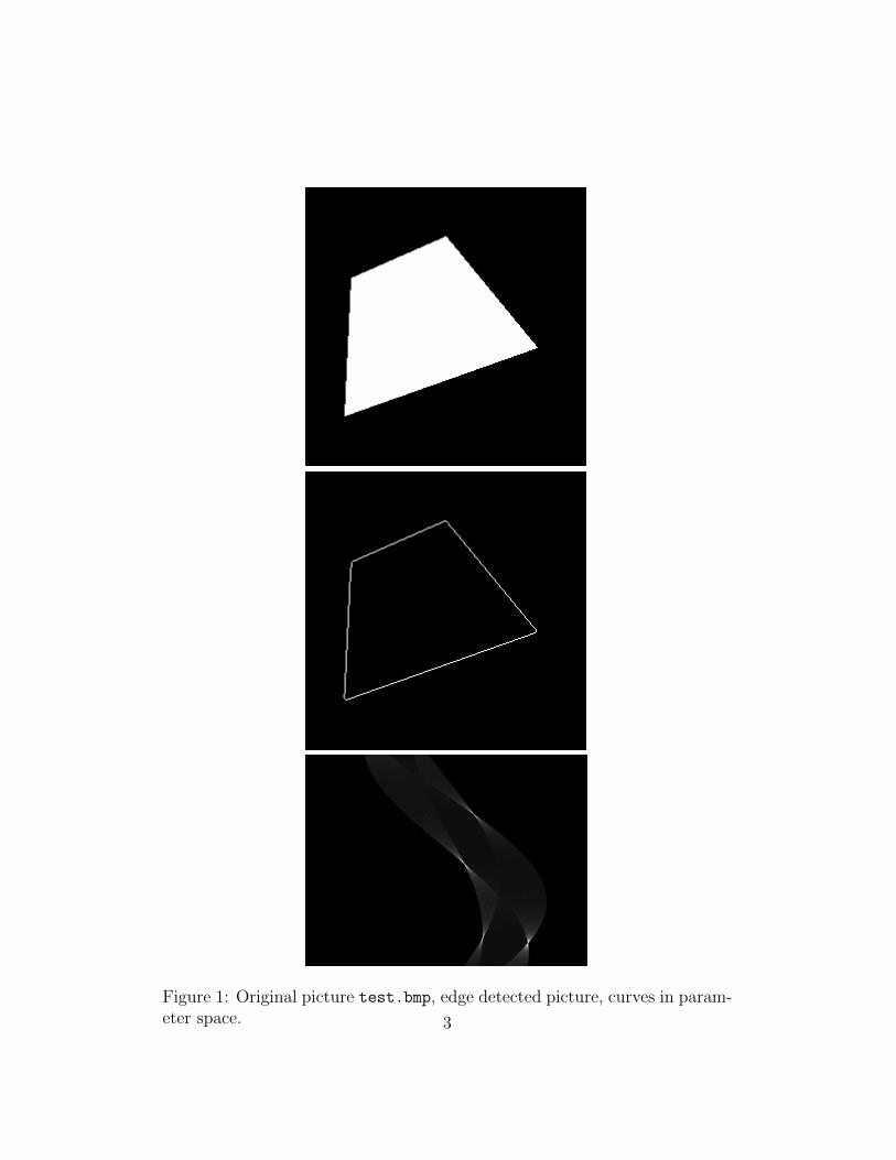
Figure 1: Original picture test.bmp, edge detected picture, curves in param-eter space. 3
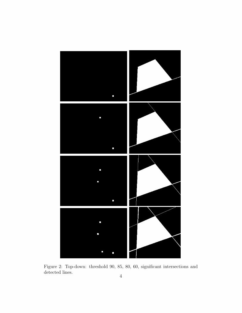
Figure 2: Top-down: threshold 90, 85, 80, 60, significant intersections anddetected lines.
4
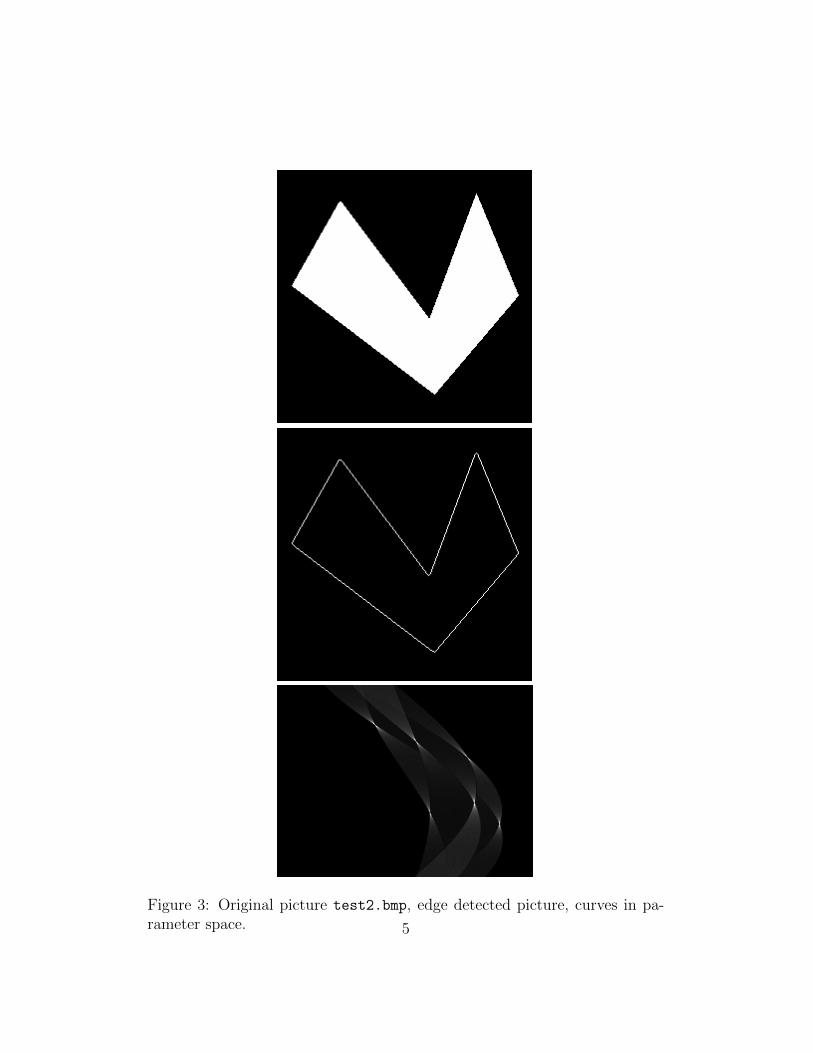
Figure 3: Original picture test2.bmp, edge detected picture, curves in pa-rameter space. 5
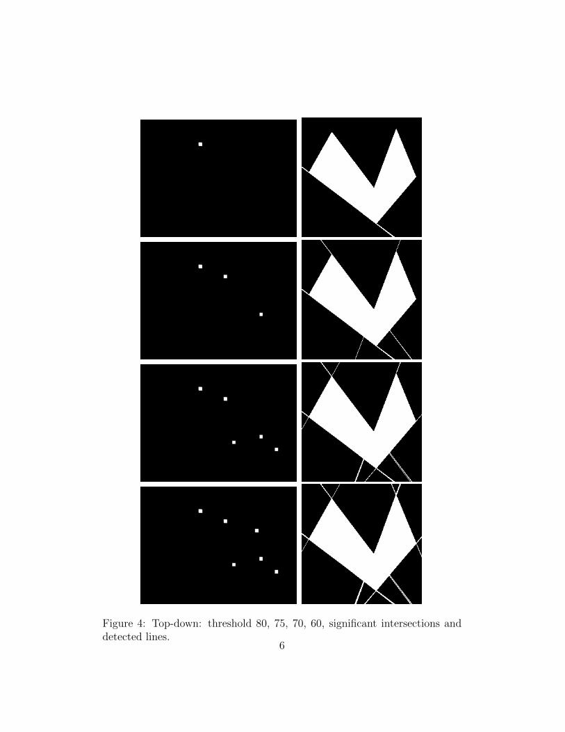
Figure 4: Top-down: threshold 80, 75, 70, 60, significant intersections anddetected lines.
6
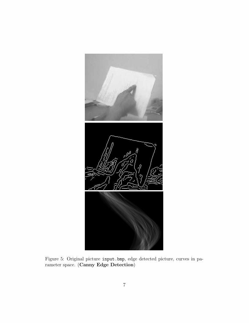
Figure 5: Original picture input.bmp, edge detected picture, curves in pa-rameter space. (Canny Edge Detection)
7
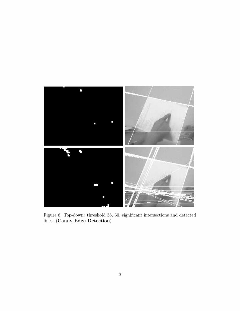
Figure 6: Top-down: threshold 38, 30, significant intersections and detectedlines. (Canny Edge Detection)
8
By using Sobel edge detector, detecting finger is still not easy, but wecan observe that Sobel edge detector achieved better result than Canny edgedetector.
I also tried different quantization scheme.I tried 768× 1024, 480× 640, 120× 180, and 30× 45.I felt that 480 × 640 gave the best results. So neither using too coarse
nor too fine quantization achieve good result.
3.4 2013 Nissan Altima 2.5 SV
I got a picture from http://savageonwheels.com/2012/09/15/2013-nissan-altima-2-5-sv/.I used ’sobel’ as the edge detector, and the accumulator got 244 as the
maximal count, as shown in Figure 12.By setting the threshold as 195, we got the detected lines, as shown in
Figure 13.The result looks good. We can observe that the edges of windshield, the
edge of front door, the edge of shift selector area and the edge of glove boxare all detected.
4 MATLAB codes
1 % main MP62 f i l ename = ’ alt ima−i n t 2 ’ ;3 picname = [ f i l ename , ’ . jpg ’ ] ;4 %5 I1 = imread ( picname ) ;6 I2 = rgb2gray ( I1 ) ;7 %8 imshow( I2 , [ 0 , 2 5 5 ] ) ;9 set ( gcf , ’ p ape r s i z e ’ , [ 5 5 ] ) ;
10 picname = [ f i l ename , ’ 1 . eps ’ ] ;11 saveas ( gcf , picname , ’ epsc ’ ) ;12 eps2pdf ( picname ) ;13 %14 % BW = edge ( I2 , ’ canny ’ ) ;15 BW = edge ( I2 , ’ s obe l ’ ) ;16 %17 imshow(BW, [ 0 , 1 ] ) ;18 set ( gcf , ’ p ape r s i z e ’ , [ 5 5 ] ) ;19 picname = [ f i l ename , ’ 2 . eps ’ ] ;
9
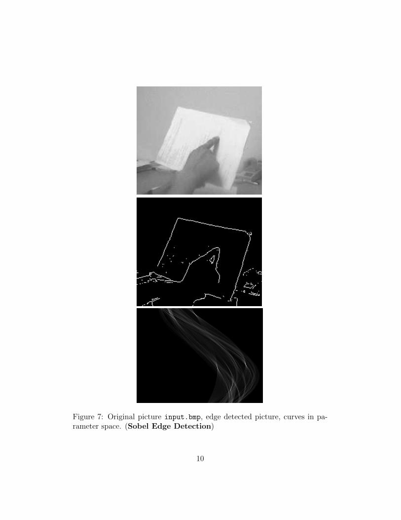
Figure 7: Original picture input.bmp, edge detected picture, curves in pa-rameter space. (Sobel Edge Detection)
10
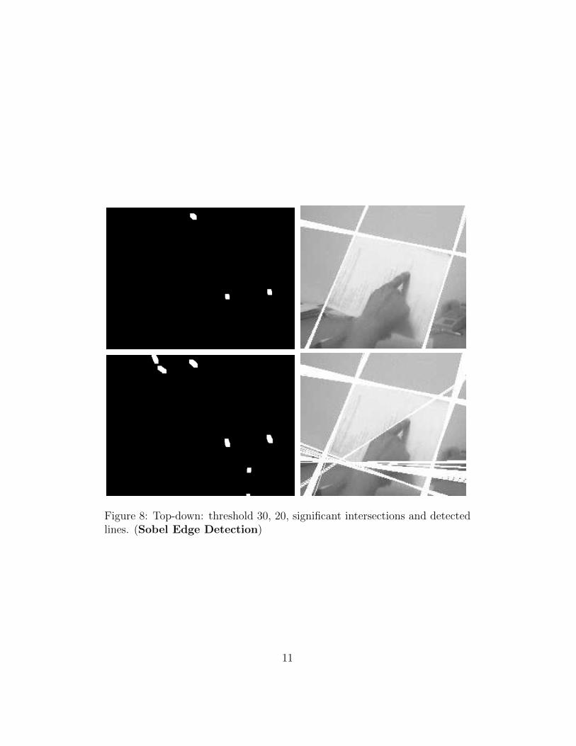
Figure 8: Top-down: threshold 30, 20, significant intersections and detectedlines. (Sobel Edge Detection)
11
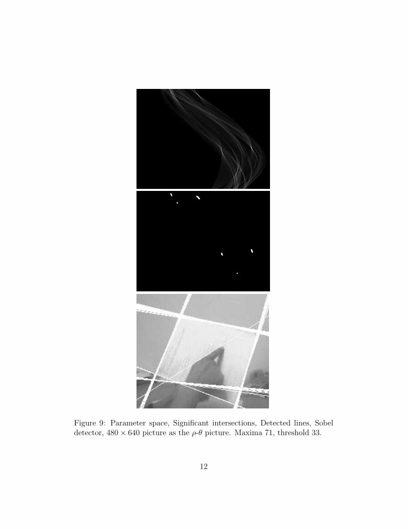
Figure 9: Parameter space, Significant intersections, Detected lines, Sobeldetector, 480× 640 picture as the ρ-θ picture. Maxima 71, threshold 33.
12
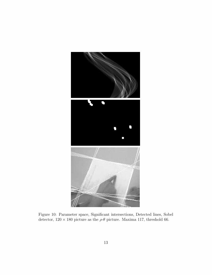
Figure 10: Parameter space, Significant intersections, Detected lines, Sobeldetector, 120× 180 picture as the ρ-θ picture. Maxima 117, threshold 66.
13
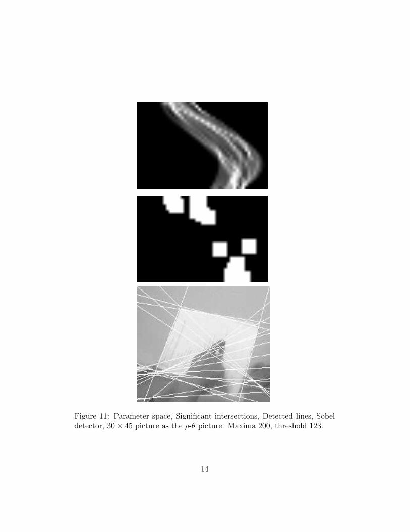
Figure 11: Parameter space, Significant intersections, Detected lines, Sobeldetector, 30× 45 picture as the ρ-θ picture. Maxima 200, threshold 123.
14
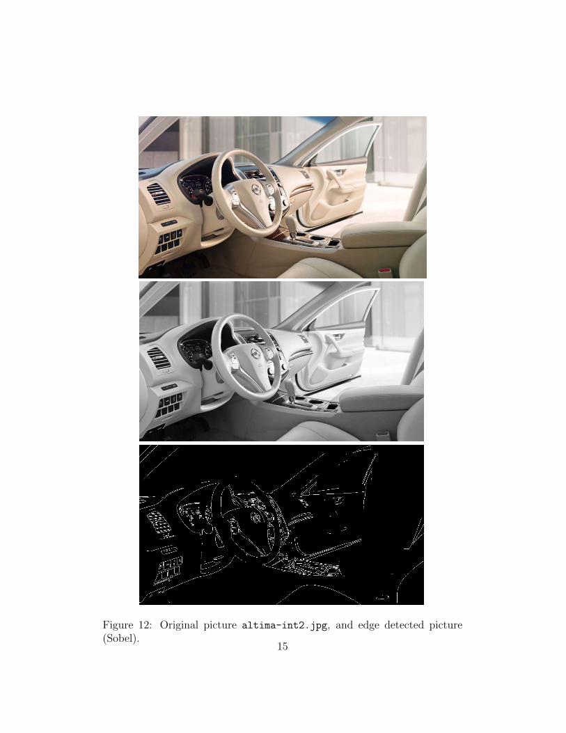
Figure 12: Original picture altima-int2.jpg, and edge detected picture(Sobel).
15
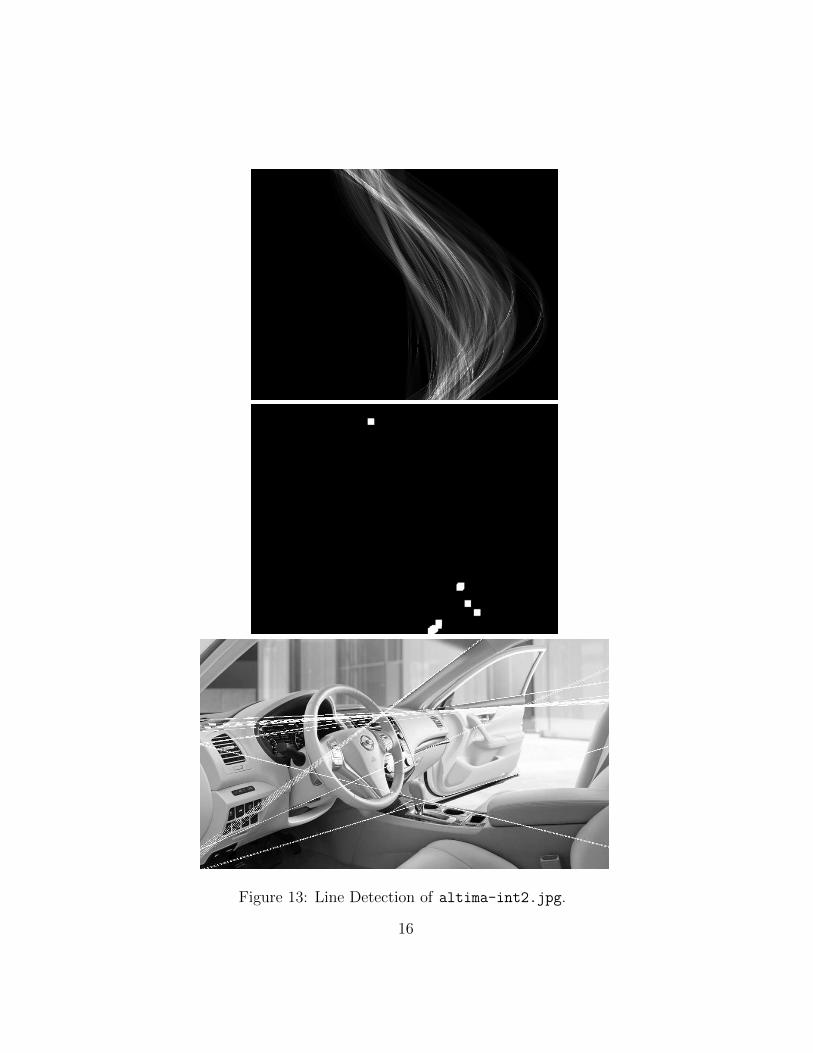
Figure 13: Line Detection of altima-int2.jpg.
16
20 saveas ( gcf , picname , ’ epsc ’ ) ;21 eps2pdf ( picname ) ;22 %23 paramTheta = 768 ;24 paramRho = 1024 ;25 midTheta = (1+paramTheta ) /2 ;26 midRho = (1+paramRho) /2 ;27 paramPic = zeros ( paramTheta , paramRho) ;28 %29 [ imY, imX ] = s ize (BW) ;30 %31 TL = −pi /2 ; TU = pi /2 ;32 RL = −sqrt (imYˆ2+imXˆ2) ;33 RU = sqrt (imYˆ2+imXˆ2) ;34 %35 for i =1:1 :imY36 for j =1:1 :imX37 i f BW( i , j ) == 138 for k=1:1: paramTheta39 theta = (k−midTheta ) /paramTheta∗pi ;40 rho = j ∗cos ( theta )+i ∗ sin ( theta ) ;41 kk = round( rho/RU∗(midRho−1) + midRho) ;42 paramPic (k , kk ) = paramPic (k , kk )+1;43 end44 end45 end46 end47 %48 maxCum = max(max( paramPic ) ) ;49 maxNum = 0 ;50 for k=1:1 : paramTheta51 for kk=1:1:paramRho52 i f paramPic (k , kk ) == maxCum53 maxNum = maxNum + 1 ;54 end55 end56 end57 %58 maxCum59 %60 %imshow( paramPic , [ 0 , round (maxCum∗0 .2) ] ) ;61 %imshow( paramPic , [ 0 , round (maxCum∗0.75) ] ) ;62 %imshow( paramPic , [ 0 , round (maxCum∗0.50) ] ) ;63 imshow( paramPic , [ 0 , round(maxCum∗0 . 75 ) ] ) ;64 set ( gcf , ’ p ape r s i z e ’ , [ 5 5 ] ) ;
17
65 picname = [ f i l ename , ’ 3 . eps ’ ] ;66 saveas ( gcf , picname , ’ epsc ’ ) ;67 eps2pdf ( picname ) ;68 %69 c r i t i c a lV a l u e = 195 ;70 count = 0 ;71 for k=1:1 : paramTheta72 for kk=1:1:paramRho73 i f paramPic (k , kk ) >= c r i t i c a lV a l u e74 count = count + 1 ;75 end76 end77 end78 count79 %80 i n c r S i z e = 10 ;81 imSig Inte r = zeros ( paramTheta , paramRho) ;82 for k=1:1 : paramTheta83 for kk=1:1:paramRho84 i f paramPic (k , kk ) >= c r i t i c a lV a l u e85 for mm = max(1 , k−i n c r S i z e ) : 1 :min( paramTheta , k+
i n c r S i z e )86 for nn = max(1 , kk−i n c r S i z e ) : 1 :min(paramRho , kk+
i n c r S i z e )87 imSig Inte r (mm, nn) = 1 ;88 end89 end90 end91 end92 end93 %94 imshow( imSigInter , [ 0 , 1 ] ) ;95 set ( gcf , ’ p ape r s i z e ’ , [ 5 5 ] ) ;96 picname = [ f i l ename , ’ 4 . eps ’ ] ;97 saveas ( gcf , picname , ’ epsc ’ ) ;98 eps2pdf ( picname ) ;99 %100 I3 = I2 ;101 for k=1:1 : paramTheta102 for kk=1:1:paramRho103 i f paramPic (k , kk ) >= c r i t i c a lV a l u e104 theta = (k−midTheta ) /paramTheta∗pi ;105 rho = (kk − midRho) /(midRho−1)∗RU;106 for i =1:1 :imY107 j = round ( ( rho−i ∗ sin ( theta ) ) /cos ( theta ) ) ;
18
108 i f j>0109 i f j<=imX110 I3 ( i , j ) = 255 ;111 end112 end113 end114 for j =1:1 :imX115 i = round ( ( rho−j ∗cos ( theta ) ) / sin ( theta ) ) ;116 i f i>0117 i f i<=imY118 I3 ( i , j ) = 255 ;119 end120 end121 end122 end123 end124 end125 imshow( I3 , [ 0 , 2 5 5 ] ) ;126 set ( gcf , ’ p ape r s i z e ’ , [ 5 5 ] ) ;127 picname = [ f i l ename , ’ 5 . eps ’ ] ;128 saveas ( gcf , picname , ’ epsc ’ ) ;129 eps2pdf ( picname ) ;
19