Embed Size (px)
Citation preview
Faculdade de Engenharia da Universidade do Porto
Wireless Mesh Networks for Smart-grids
Ivo Tiago da Silva Leitão
Mestrado Integrado em Engenharia Electrotécnica e de Computadores Major Telecomunicações
Orientador: Prof. Manuel Ricardo Co-orientador: Eng. Mohammad Abdellatif
Outubro 2012

ii
© Ivo Leitão, 2012

iii
Resumo
Wireless Sensor Networks é considerada uma das áreas com maior potencial dentro da
chamada “Internet das Coisas”, providenciando várias aplicações para as mais variadas áreas,
tais como monitoração industrial ou ambiental, cuidados de saúde pessoais, automação de
casas e edifícios ou aplicações de medição inteligente. Contudo, sendo estas tecnologias
ainda algo recentes, vários desafios são ainda encontrados. Nos últimos anos tem-se vindo a
assistir a um aumento do esforço em providenciar standards de forma a unificar as várias
soluções então existentes, bem como aumentar a interoperabilidade com outras redes. O
objetivo desta dissertação consiste em avaliar a performance de duas implementações
diferentes de Wireless Sensor Networks, usando protocolos como IEEE 802.15.4, 6LoWPAN,
RPL, software baseado no Sistema Operativo Contiki e um ambiente de comunicação em
multi-hop.

iv
v
Abstract
Wireless sensor networks is considered one of the areas with more potential in the
“Internet of Things”, providing several applications for the most varied areas, such as
industrial and environment monitoring, personal health care, home and building automation
or smart-metering. However, since these are still recent technologies, several issues are still
being found. In the last years there’s been a greater effort to provide standards to unify the
several different solutions available, and increase the interoperability with other networks.
The objective of this Dissertation is to evaluate the performance of two different Wireless
Sensors Networks implementations, using protocols such as IEEE 802.15.4, 6LoWPAN, RPL,
software based on the Contiki Operating System and a multi-hop communication environment.

vi
vii
Acknowledgements
I would like to thank my coordinators Prof. Manuel Ricardo and Eng. Mohammad Abdellatif
for all the time and help offered in the writing of this document.

viii
ix
Index
Resumo ............................................................................................ iii
Abstract ............................................................................................. v
Acknowledgements .............................................................................. vii
Index ............................................................................................... ix
List of figures ..................................................................................... xi
List of tables ...................................................................................... xv
Acronyms ........................................................................................ xvii
Chapter 1 ........................................................................................... 1
Introduction ....................................................................................................... 1
Chapter 2 ........................................................................................... 3
State of the Art .................................................................................................. 3 2.1 Solutions Research ..................................................................................... 3 2.1.1 Contiki+6LoWPAN+RPL ................................................................................ 3 2.1.2 TinyOS+6LoWPAN+RPL ................................................................................ 4 2.1.3 Contiki and TinyOS comparison ..................................................................... 5 2.1.4 Low-power WiFi WSN’s ................................................................................ 7 2.1.5 ZigBee device: Bytesnap ZMM-01 ................................................................... 9 2.2 Technologies research .............................................................................. 11 2.2.1 IEEE 802.15.4-2006 .................................................................................. 11 2.2.2 6LoWPAN .............................................................................................. 14 2.2.3 RPL 16 2.2.4 IEEE 802.11 ............................................................................................ 19 2.2.5 ZigBee .................................................................................................. 21 2.2.6 Advanticsys MTM-CM5000-MSP sensor mote ..................................................... 23
Chapter 3 .......................................................................................... 25
Self-PVP Project ................................................................................................ 25 3.1 System Description .................................................................................. 25 3.2 Methodology .......................................................................................... 27 3.2.1 Technique 1 ........................................................................................... 28 3.2.2 Technique 2 ........................................................................................... 29
x
3.2.3 Technique 3 ........................................................................................... 30 3.3 Results and discussion .............................................................................. 31 3.3.1 Technique 1 ........................................................................................... 34 3.3.2 Technique 3 ........................................................................................... 36 3.3.3 Technique 2 ........................................................................................... 38
Chapter 4 .......................................................................................... 41
Smart Electric Counters Project ............................................................................ 41 4.1 System Description .................................................................................. 41 4.2 Methodology .......................................................................................... 45 4.3 Results and discussion .............................................................................. 52 4.3.1 Preliminary Results .................................................................................. 52 4.3.2 Cooja simulations results ........................................................................... 54 4.3.3 Cooja simulations with 2 simultaneous processes results .................................... 56
Chapter 5 .......................................................................................... 59
Conclusions ..................................................................................................... 59
References ........................................................................................ 61
xi
List of figures
Figure 1 - The Contiki Architecture......................................................................... 4
Figure 2 - The TinyOS 6LoWPAN/RPL Stack ............................................................... 5
Figure 3 - Results of tests performed on three 6LoWPAN implementations. At the left, the time to send an UDP message, at the right, the energy required to send the same messages. ................................................................................................. 6
Figure 4 - Average packet reception ratios for Tiny RPL (left) and Contiki RPL (right) ........... 7
Figure 5 - GS1011 Hardware description ................................................................... 8
Figure 6 - Redpine Signals SenSiFi hardware architecture ............................................. 9
Figure 7 - Bytesnap ZMM-01 Device ....................................................................... 10
Figure 8 - Basic topologies for 802.15.4 ................................................................. 11
Figure 9 - Cluster tree topology for 802.15.4 ........................................................... 12
Figure 10 - Communication in a beacon enabled PAN ................................................. 13
Figure 11 - 6LoWPAN Architecture ........................................................................ 14
Figure 12 - RFC6282 Header compression example .................................................... 15
Figure 13 - Typical Neighbor Discovery message exchange .......................................... 16
Figure 14 - RPL Architecture ............................................................................... 17
Figure 15 - RPL Node Rank ................................................................................. 18
Figure 16 - IEEE 802.11 Operation modes ............................................................... 19
Figure 17 - The hidden node problem .................................................................... 21
Figure 18 - Zigbee Stack Architecture ................................................................... 21
Figure 19 - Block diagram for TelosB general architecture .......................................... 23
Figure 20 - System Topology ............................................................................... 26
Figure 21 - Network topology .............................................................................. 27
xii
Figure 22 - Technique 1 .................................................................................... 28
Figure 23 - Technique 1 initialization .................................................................... 29
Figure 24 - Technique 2 .................................................................................... 30
Figure 25 - Technique 3 .................................................................................... 30
Figure 26 - Incorrect routing table ....................................................................... 31
Figure 27 - Motes position used to perform the tests in this chapter. ............................. 32
Figure 28 - Average packet loss for Technique 1 ....................................................... 34
Figure 29 - Throughput for Technique 1 ................................................................. 35
Figure 30 - Average packet loss for Technique 3 ....................................................... 36
Figure 31 - Average throughput for Technique 3 ....................................................... 37
Figure 32 - Preliminary packet loss for Technique 2 .................................................. 38
Figure 33 - Preliminary throughput for Technique 2 .................................................. 39
Figure 34 - Throughput for Technique 2 ................................................................. 40
Figure 35 - Application scenario .......................................................................... 42
Figure 36 - RPL-Border Router webpage ................................................................. 43
Figure 37 - Sensor mote homepage ....................................................................... 43
Figure 38 - Screenshot of the sensing data charts available at each sensor mote ............... 44
Figure 39 - Network map. The IPv6 Addresses are tunslip6/Cooja generated .................... 45
Figure 40 - tunslip6 initialization ......................................................................... 46
Figure 41 - Algorithm for script to run HTTP and ping6 requests ................................... 47
Figure 42 - wget HTTP delay measurement process ................................................... 48
Figure 43 - Effective delay for HTTP requests calculation technique .............................. 49
Figure 44 - An example from a wget log file ............................................................ 50
Figure 45 - Differences from script 1 to script 2 ....................................................... 51
Figure 46 - Screenshot from shell window running the script ....................................... 51
Figure 47 - HTTP request delay and average number of connection attempts for each node, using a Contiki 2.5 based configuration ................................................... 52
Figure 48 - Average number of connection attempts using a contiki 2.5 based configuration but with a maximum 1 TCP connection allowed per node ................... 53
Figure 49 - Plot for the HTTP requests delay simulated in Cooja with Contiki 2.6 .............. 54
Figure 50- Plot for the PING6 requests delay simulated in Cooja with Contiki 2.6 .............. 55
xiii
Figure 51 - Delay for HTTP requests with 2 simultaneous scripts ................................... 57
Figure 52 - Average number of connection attempts per node ...................................... 57
Figure 53 - Packet loss for ping6 requests ............................................................... 58

xiv
xv
List of tables
Table 1 - Comparison of 6LoWPAN implementations .................................................... 6
Table 2 - Comparison of classic and low-power Wi-Fi performance values ......................... 8
Table 3 - PHY modes for 802.15.4-2006 ................................................................. 12
Table 4 - IEEE 802.11 protocols comparison ............................................................ 20
Table 5 - Advanticsys MTM-CM5000-MSP general characteristics .................................... 24
Table 6 - Packet loss and Throughput results for Technique 1 ...................................... 34
Table 7 - Average test time for Technique 1 ........................................................... 35
Table 8 - Packet loss and Throughput results for Technique 3 ...................................... 36
Table 9 - Average test time for Technique 3 ........................................................... 37
Table 10 - Preliminary Results for Technique 2 ........................................................ 38
Table 11 - Packet loss and throughput results for Technique 2 ..................................... 39
Table 12 - Average test times for Technique 2 ......................................................... 40
Table 13 - Obtained values for the HTTP requests in the Cooja simulation tests running on Contiki 2.6 .............................................................................................. 54
Table 14 - Obtained values for the ping6 messages in the Cooja simulation tests running on Contiki 2.6 .......................................................................................... 55
Table 15 - Obtained values for the HTTP requests in the Cooja simulation tests running on Contiki 2.6 with 2 simultaneous processes ....................................................... 56
Table 16 - Results for ping6 requests with 2 simultaneous processes .............................. 58

xvi
xvii
Acronyms
List of acronyms (ordered alphabetically)
6LoWPAN – IPv6 over Low Power Wireless Personal Network
AES – Advanced Encryption Standard
AODV – Ad-hoc On-Demand Distance Vector Routing
CAP – Contention Access Period
CFP – Contention Free Period
CSMA/CA – Carrier Sense Multiple Access with Collision Avoidance
CTS – Clear to Send
DCF - Distributed Coordination Function
DODAG - Destination-Oriented Directed Acyclic Graph
DSSS – Direct Sequence Spread Spectrum
DYMO – Dynamic MANET On-Demand
FFD – Full Function Device
FHSS – Frequency Hopping Spread Spectrum
GTS – Guaranteed Time Slot
HTTP – Hypertext Transfer Protocol
ICMP - Internet Control Message Protocol
IEEE – Institute of Electrical and Electronics Engineers
IETF – Internet Engineering Task Force
IFS - Inter-Frame Space
INESC – Instituto de Engenharia de Sistemas e Computadores
IP – Internet Protocol
LLN – Low Power, Lossy Network
MAC – Medium Access Control
MIMU – Multiple-Input, Multiple-Output
MTU – Maximum Transfer Unit
OFDM – Orthogonal Frequency Division Multiplexing
PAN – Personal Area Network

xviii
PCF - Point Coordination Function
PHY – Physical Layer
RFD – Reduced Function Device
RPL - Routing Protocol for Low Power Lossy Networks
RTS – Request to Send
SICS - Swedish Institute of Computer Science
SELF-PVP - Self-organizing power management for photo-voltaic power plants
SLIP - Serial Line Internet Protocol
TCP – Transmission Control Protocol
UDP – User Datagram Protocol
USB – Universal Serial Bus
Chapter 1
Introduction
Communication networks have been experiencing a great development over the past few
years. One of such areas is the area of “The Internet of Things”, where embedded “smart
objects” devices are becoming an important part of the Internet. Wireless Sensor Networks
(WSNs) is one area with an immense potential in future applications. Industrial “machine
health” monitoring and automation, environmental monitoring of areas such as volcanos and
forests, personal healthcare devices, tracking devices for objects and people and smart
energy metering applications are examples of areas where the “Internet of Things” and WSNs
can be applied.
Wireless Sensor Networks consist of several small and highly power-efficient (often
battery powered) wireless devices capable of communicating sensor data using low-power
and low-bandwidth links often in an autonomous fashion, through a root or a sink node. Since
the 1990s until early 2000s several proprietary wireless and low-power networking
technologies have surfaced, but it was only in 2003 that the Institute of Electrical and
Electronic Engineers (IEEE) released the first low-power wireless personal area network
(WPAN) standard: IEEE 802.15.4, defining the Physical and Medium Access Control layers from
the OSI model. Based on that standard, ZigBee Alliance developed its own specification for
the higher layers, providing commercial wireless embedded networking solutions for various
areas. Other specifications based on IEEE 802.15.4 have surfaced as well, such as ISA100.11a
and WirelessHART. However these proprietary solutions still have problems regarding the
scalability and Internet Integration. IP is the de-facto Internet layer protocol widely used in
the Internet today, and most of the WSN solutions didn’t provide IP support, often using
special designed gateways to provide interoperability across WSNs and outside networks. With
the appearance of IPv6 and the 3.4×1038 different addresses it supports, the addressing space
to support billions of embedded devices is now available. However, the complexity of
providing IPv6 for highly memory and processing constrained devices has become a
formidable challenge. IETF has assigned two different task groups to integrate IPv6 on WSN
devices: 6LoWPAN is the adaptation layer for IPv6 packets on IEEE 802.15.4 MAC messages,
while RPL provides power-efficient routing mechanisms.
2 Introduction
2
Beside closed-group commercial solutions, there are other “open source” solutions
regarding WSNs. Operating systems for embedded devices such as TinyOS and Contiki are
open-source and provide implementations of the IEEE 802.15.4, IETF 6LoWPAN and RPL
routing for several different memory and power constrained devices. These approaches offer
more freedom in developing solutions for specific network requirements.
Recently there’s been an adaptation of IEEE 802.11 protocols towards WSNs. While Wi-Fi
devices are targeted for non-power restricted and high data-rate, reliable networks,
traditional Wi-Fi devices were not an efficient solution to deploy WSNs. However, several
manufacturers have started to produce highly efficient 802.11 compliant devices, with
power-consumptions close to the IEEE 802.15.4 counterparts, with the higher data-rates and
the mature interoperability of IEEE 802.11 devices. Although this “low-power WiFi” is still a
very recent technology and not fully tested, it is an interesting alternative that will be more
described in the next chapters.
This Dissertation will cover two different analyses. The first is a confirmation of
simulation results by Mohammad Abdellatif covered by his paper, while the second problem
addressed relies on the Contiki Operating system communication stack and how its
parameters affect the communication performance for TCP through HTTP requests and ICMP
messages. Chapter 2 is dedicated to the state of the art research, being divided on two
different sections. The first section describes some solutions found that are able to tackle the
Dissertation’s problems, while the second section describes the technologies that are behind
those solutions. Chapter 3 and Chapter 4 cover the Dissertation different projects. Chapter 3
is related to Mohammad Abdellatif’s Ph.D work on the Self-PVP Project, in which three data
collection techniques are analyzed, while Chapter 4 covers the Smart Electric Counters
Project. Both chapters are divided in three different sections, one for the system description,
another for the methodology followed for proceeding with the tests, and the final section
providing the results and discussion. Finally, Chapter 5 concludes and suggests future work.
Chapter 2
State of the Art
2.1 Solutions Research
In this chapter, some commercial solutions to address the Dissertation objective will be
listed and detailed. On the first part, solutions using open source Operating Systems on motes
operating in IEEE 802.15.4 standard will be addressed, such as Contiki and TinyOS. The
second part will compare the 6LoWPAN and RPL implementations of the former sensor nodes
operating systems. The third part will detail some commercial solutions found using low
power WiFi architectures. Finally, the last part in this chapter will briefly mention other
solutions available using other technologies such as ZigBee.
2.1.1 Contiki+6LoWPAN+RPL
Contiki is an open source operating system designed for memory-constrained devices,
from embedded microcontroller systems to wireless sensor network motes. Its development
was started by Adam Dunkels of the Networked Embedded Systems Group at the Swedish
Institute of Computer Science (SICS), and since then several other developers worked on the
OS to provide it several new features.
The Contiki OS general features are as follows:
Full IPv4 and IPv6 support for IP communication, using the uIPv6 Stack.
It has a multitasking kernel, with support for multithreading programming using
pre-emptive multithreading and protothreads.
Power efficient radio and network mechanisms, 6lowpan header compression, RPL
routing and CoAP application layer protocol.
Included applications such as an HTTP server and Telnet client
4 State of the Art
4
Supports several simulators such as Cooja, to aid in the software development
and debugging process.
A proprietary file system for data storage
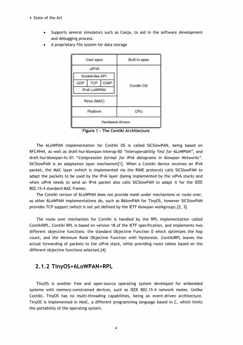
Figure 1 - The Contiki Architecture
The 6LoWPAN implementation for Contiki OS is called SICSlowPAN, being based on
RFC4944, as well as draft-hui-6lowpan-interop-00 “Interoperability Test for 6LoWPAN”, and
draft-hui-6lowpan-hc-01 “Compression format for IPv6 datagrams in 6lowpan Networks”.
SICSlowPAN is an adaptation layer mechanism[1]. When a Contiki device receives an IPv6
packet, the MAC layer (which is implemented via the RIME protocol) calls SICSlowPAN to
adapt the packets to be used by the IPv6 layer (being implemented by the uIPv6 stack) and
when uIPv6 needs to send an IPv6 packet also calls SICSlowPAN to adapt it for the IEEE
802.15.4 standard MAC frames.
The Contiki version of 6LoWPAN does not provide mesh under mechanisms or route over,
as other 6LoWPAN implementations do, such as B6lowPAN for TinyOS, however SICSlowPAN
provides TCP support (which is not yet defined by the IETF 6lowpan workgroup).[2, 3]
The route over mechanism for Contiki is handled by the RPL implementation called
ContikiRPL. Contiki RPL is based on version 18 of the IETF specification, and implements two
different objective functions: the standard Objective Function 0 which optimizes the hop
count, and the Minimum Rank Objective Function with Hysteresis. ContikiRPL leaves the
actual forwarding of packets to the uIPv6 stack, while providing route tables based on the
different objective functions selected.[4]
2.1.2 TinyOS+6LoWPAN+RPL
TinyOS is another free and open-source operating system developed for embedded
systems with memory-constrained devices, such as IEEE 802.15.4 network motes. Unlike
Contiki, TinyOS has no multi-threading capabilities, being an event-driven architecture.
TinyOS is implemented in NesC, a different programming language based in C, which limits
the portability of the operating system.
Solutions research 5
5
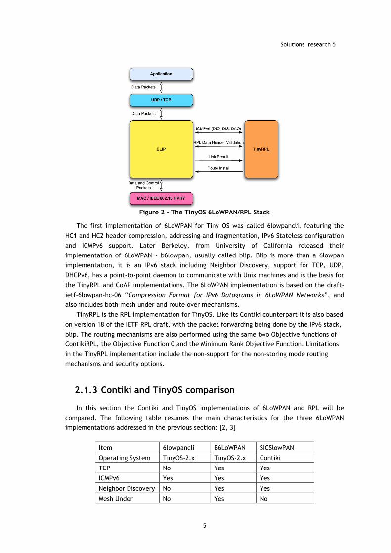
Figure 2 - The TinyOS 6LoWPAN/RPL Stack
The first implementation of 6LoWPAN for Tiny OS was called 6lowpancli, featuring the
HC1 and HC2 header compression, addressing and fragmentation, IPv6 Stateless configuration
and ICMPv6 support. Later Berkeley, from University of California released their
implementation of 6LoWPAN - b6lowpan, usually called blip. Blip is more than a 6lowpan
implementation, it is an IPv6 stack including Neighbor Discovery, support for TCP, UDP,
DHCPv6, has a point-to-point daemon to communicate with Unix machines and is the basis for
the TinyRPL and CoAP implementations. The 6LoWPAN implementation is based on the draft-
ietf-6lowpan-hc-06 “Compression Format for IPv6 Datagrams in 6LoWPAN Networks”, and
also includes both mesh under and route over mechanisms.
TinyRPL is the RPL implementation for TinyOS. Like its Contiki counterpart it is also based
on version 18 of the IETF RPL draft, with the packet forwarding being done by the IPv6 stack,
blip. The routing mechanisms are also performed using the same two Objective functions of
ContikiRPL, the Objective Function 0 and the Minimum Rank Objective Function. Limitations
in the TinyRPL implementation include the non-support for the non-storing mode routing
mechanisms and security options.
2.1.3 Contiki and TinyOS comparison
In this section the Contiki and TinyOS implementations of 6LoWPAN and RPL will be
compared. The following table resumes the main characteristics for the three 6LoWPAN
implementations addressed in the previous section: [2, 3]
Item 6lowpancli B6LoWPAN SICSlowPAN
Operating System TinyOS-2.x TinyOS-2.x Contiki
TCP No Yes Yes
ICMPv6 Yes Yes Yes
Neighbor Discovery No Yes Yes
Mesh Under No Yes No
6 State of the Art
6
Route Over No Yes No (Contiki RPL)
Table 1 - Comparison of 6LoWPAN implementations
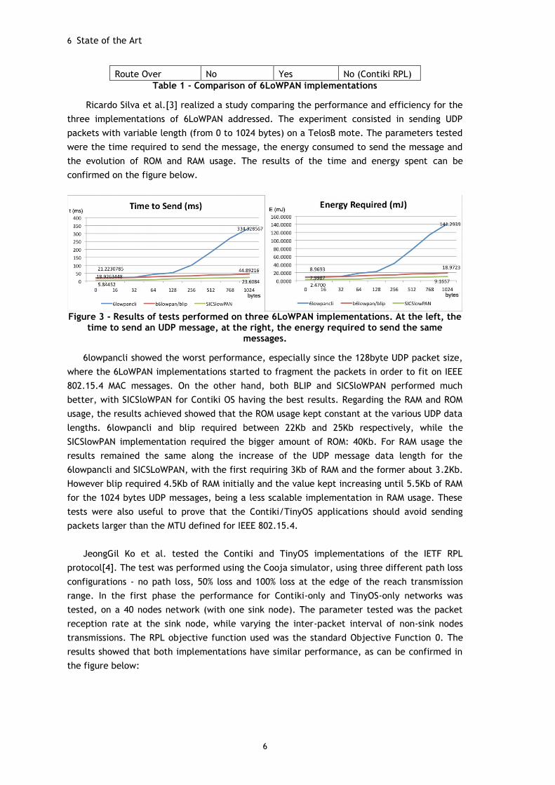
Ricardo Silva et al.[3] realized a study comparing the performance and efficiency for the
three implementations of 6LoWPAN addressed. The experiment consisted in sending UDP
packets with variable length (from 0 to 1024 bytes) on a TelosB mote. The parameters tested
were the time required to send the message, the energy consumed to send the message and
the evolution of ROM and RAM usage. The results of the time and energy spent can be
confirmed on the figure below.
Figure 3 - Results of tests performed on three 6LoWPAN implementations. At the left, the
time to send an UDP message, at the right, the energy required to send the same messages.
6lowpancli showed the worst performance, especially since the 128byte UDP packet size,
where the 6LoWPAN implementations started to fragment the packets in order to fit on IEEE
802.15.4 MAC messages. On the other hand, both BLIP and SICSloWPAN performed much
better, with SICSloWPAN for Contiki OS having the best results. Regarding the RAM and ROM
usage, the results achieved showed that the ROM usage kept constant at the various UDP data
lengths. 6lowpancli and blip required between 22Kb and 25Kb respectively, while the
SICSlowPAN implementation required the bigger amount of ROM: 40Kb. For RAM usage the
results remained the same along the increase of the UDP message data length for the
6lowpancli and SICSLoWPAN, with the first requiring 3Kb of RAM and the former about 3.2Kb.
However blip required 4.5Kb of RAM initially and the value kept increasing until 5.5Kb of RAM
for the 1024 bytes UDP messages, being a less scalable implementation in RAM usage. These
tests were also useful to prove that the Contiki/TinyOS applications should avoid sending
packets larger than the MTU defined for IEEE 802.15.4.
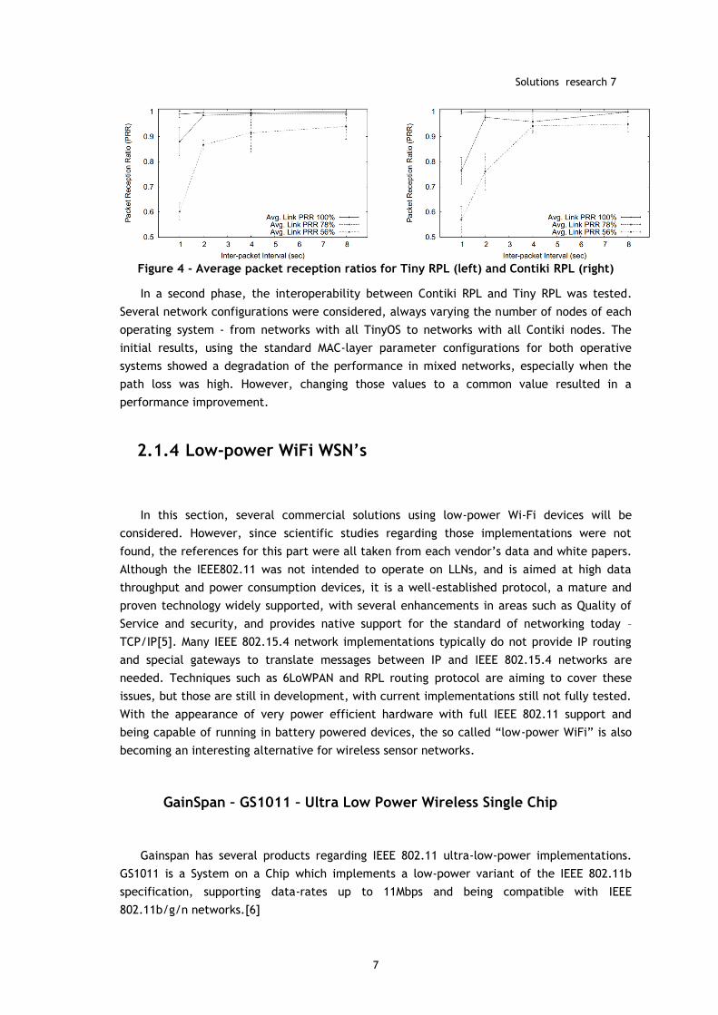
JeongGil Ko et al. tested the Contiki and TinyOS implementations of the IETF RPL
protocol[4]. The test was performed using the Cooja simulator, using three different path loss
configurations - no path loss, 50% loss and 100% loss at the edge of the reach transmission
range. In the first phase the performance for Contiki-only and TinyOS-only networks was
tested, on a 40 nodes network (with one sink node). The parameter tested was the packet
reception rate at the sink node, while varying the inter-packet interval of non-sink nodes
transmissions. The RPL objective function used was the standard Objective Function 0. The
results showed that both implementations have similar performance, as can be confirmed in
the figure below:
Solutions research 7
7
Figure 4 - Average packet reception ratios for Tiny RPL (left) and Contiki RPL (right)
In a second phase, the interoperability between Contiki RPL and Tiny RPL was tested.
Several network configurations were considered, always varying the number of nodes of each
operating system - from networks with all TinyOS to networks with all Contiki nodes. The
initial results, using the standard MAC-layer parameter configurations for both operative
systems showed a degradation of the performance in mixed networks, especially when the
path loss was high. However, changing those values to a common value resulted in a
performance improvement.
2.1.4 Low-power WiFi WSN’s
In this section, several commercial solutions using low-power Wi-Fi devices will be
considered. However, since scientific studies regarding those implementations were not
found, the references for this part were all taken from each vendor’s data and white papers.
Although the IEEE802.11 was not intended to operate on LLNs, and is aimed at high data
throughput and power consumption devices, it is a well-established protocol, a mature and
proven technology widely supported, with several enhancements in areas such as Quality of
Service and security, and provides native support for the standard of networking today –
TCP/IP[5]. Many IEEE 802.15.4 network implementations typically do not provide IP routing
and special gateways to translate messages between IP and IEEE 802.15.4 networks are
needed. Techniques such as 6LoWPAN and RPL routing protocol are aiming to cover these
issues, but those are still in development, with current implementations still not fully tested.
With the appearance of very power efficient hardware with full IEEE 802.11 support and
being capable of running in battery powered devices, the so called “low-power WiFi” is also
becoming an interesting alternative for wireless sensor networks.
GainSpan – GS1011 – Ultra Low Power Wireless Single Chip
Gainspan has several products regarding IEEE 802.11 ultra-low-power implementations.
GS1011 is a System on a Chip which implements a low-power variant of the IEEE 802.11b
specification, supporting data-rates up to 11Mbps and being compatible with IEEE
802.11b/g/n networks.[6]
8 State of the Art
8
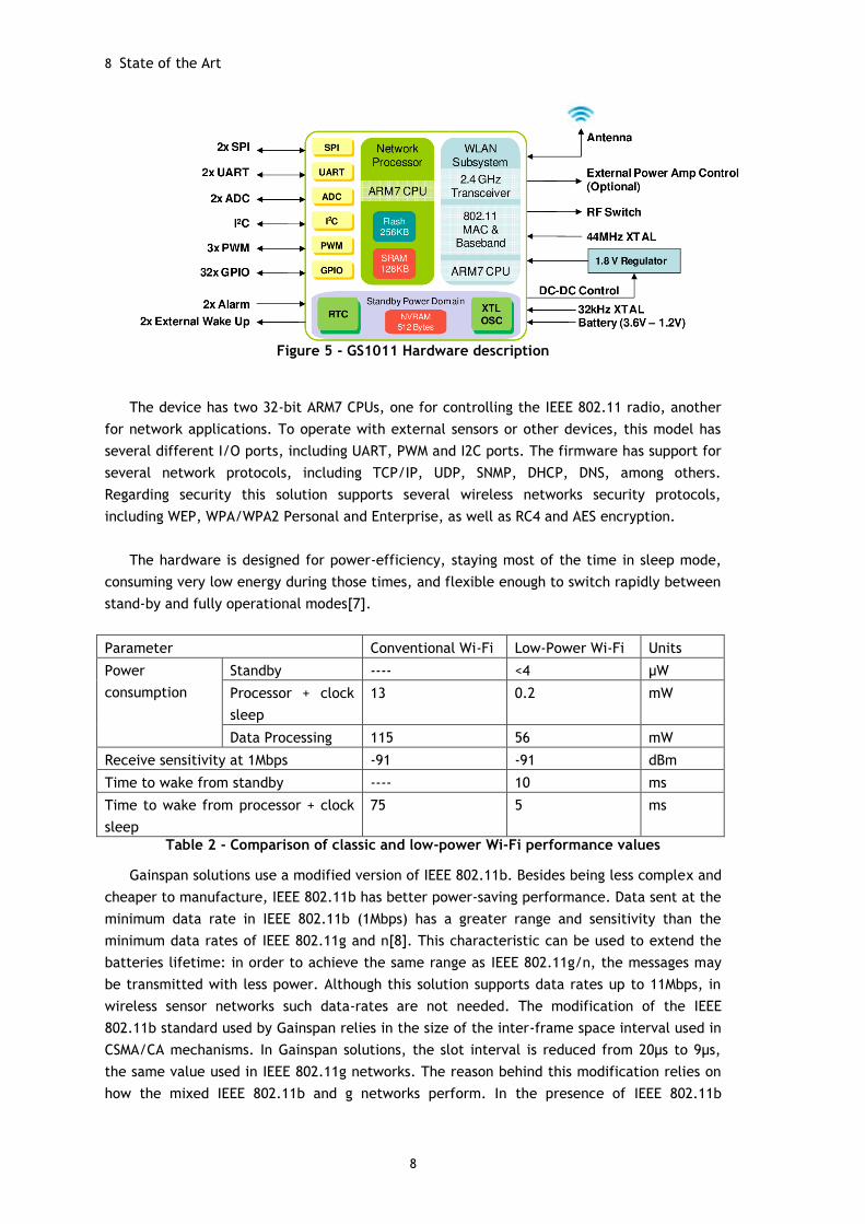
Figure 5 - GS1011 Hardware description
The device has two 32-bit ARM7 CPUs, one for controlling the IEEE 802.11 radio, another
for network applications. To operate with external sensors or other devices, this model has
several different I/O ports, including UART, PWM and I2C ports. The firmware has support for
several network protocols, including TCP/IP, UDP, SNMP, DHCP, DNS, among others.
Regarding security this solution supports several wireless networks security protocols,
including WEP, WPA/WPA2 Personal and Enterprise, as well as RC4 and AES encryption.
The hardware is designed for power-efficiency, staying most of the time in sleep mode,
consuming very low energy during those times, and flexible enough to switch rapidly between
stand-by and fully operational modes[7].
Parameter Conventional Wi-Fi Low-Power Wi-Fi Units
Power
consumption
Standby ---- <4 µW
Processor + clock
sleep
13 0.2 mW
Data Processing 115 56 mW
Receive sensitivity at 1Mbps -91 -91 dBm
Time to wake from standby ---- 10 ms
Time to wake from processor + clock
sleep
75 5 ms
Table 2 - Comparison of classic and low-power Wi-Fi performance values
Gainspan solutions use a modified version of IEEE 802.11b. Besides being less complex and
cheaper to manufacture, IEEE 802.11b has better power-saving performance. Data sent at the
minimum data rate in IEEE 802.11b (1Mbps) has a greater range and sensitivity than the
minimum data rates of IEEE 802.11g and n[8]. This characteristic can be used to extend the
batteries lifetime: in order to achieve the same range as IEEE 802.11g/n, the messages may
be transmitted with less power. Although this solution supports data rates up to 11Mbps, in
wireless sensor networks such data-rates are not needed. The modification of the IEEE
802.11b standard used by Gainspan relies in the size of the inter-frame space interval used in
CSMA/CA mechanisms. In Gainspan solutions, the slot interval is reduced from 20µs to 9µs,
the same value used in IEEE 802.11g networks. The reason behind this modification relies on
how the mixed IEEE 802.11b and g networks perform. In the presence of IEEE 802.11b
Solutions research 9
9
devices, IEEE 802.11g devices use IEEE 802.11b slot intervals to communicate with 11b
devices. Using 11g slot times, the maximum throughput in a mixed b and g network can be
maximized.
Redpine Signals – SenSiFi 802.11n Sensor Network Module
Redpine Signals has several products with low-power WiFi technology. The SenSiFi module
(referenced as RS9110-N-11-31) is a sensor node compatible with IEEE 802.11b/g/n
specifications, while only operates on a single stream for IEEE 802.11n with a maximum data
rate of 65Mbps. The SenSiFi module also implements IEEE 802.11i specifications for Wireless
security, such as AES encryption, WEP, TKIP, WPA and WPA2[9].
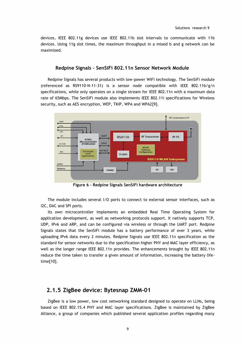
Figure 6 - Redpine Signals SenSiFi hardware architecture
The module includes several I/O ports to connect to external sensor interfaces, such as
I2C, DAC and SPI ports.
Its own microcontroller implements an embedded Real Time Operating System for
application development, as well as networking protocols support. It natively supports TCP,
UDP, IPv6 and ARP, and can be configured via wireless or through the UART port. Redpine
Signals states that the SenSiFi module has a battery performance of over 3 years, while
uploading IPv6 data every 2 minutes. Redpine Signals use IEEE 802.11n specification as the
standard for sensor networks due to the specification higher PHY and MAC layer efficiency, as
well as the longer range IEEE 802.11n provides. The enhancements brought by IEEE 802.11n
reduce the time taken to transfer a given amount of information, increasing the battery life-
time[10].
2.1.5 ZigBee device: Bytesnap ZMM-01
ZigBee is a low power, low cost networking standard designed to operate on LLNs, being
based on IEEE 802.15.4 PHY and MAC layer specifications. ZigBee is maintained by ZigBee
Alliance, a group of companies which published several application profiles regarding many
10 State of the Art
10
different areas, from Home and Building Automation, Health Care to Smart Energy control
and metering. One of the many companies releasing ZigBee Certified Products is Bytesnap.
The ZMM-01 device is a ZigBee Smart Energy module, designed to act as metering electric
device and controller for several different application scenarios[11].
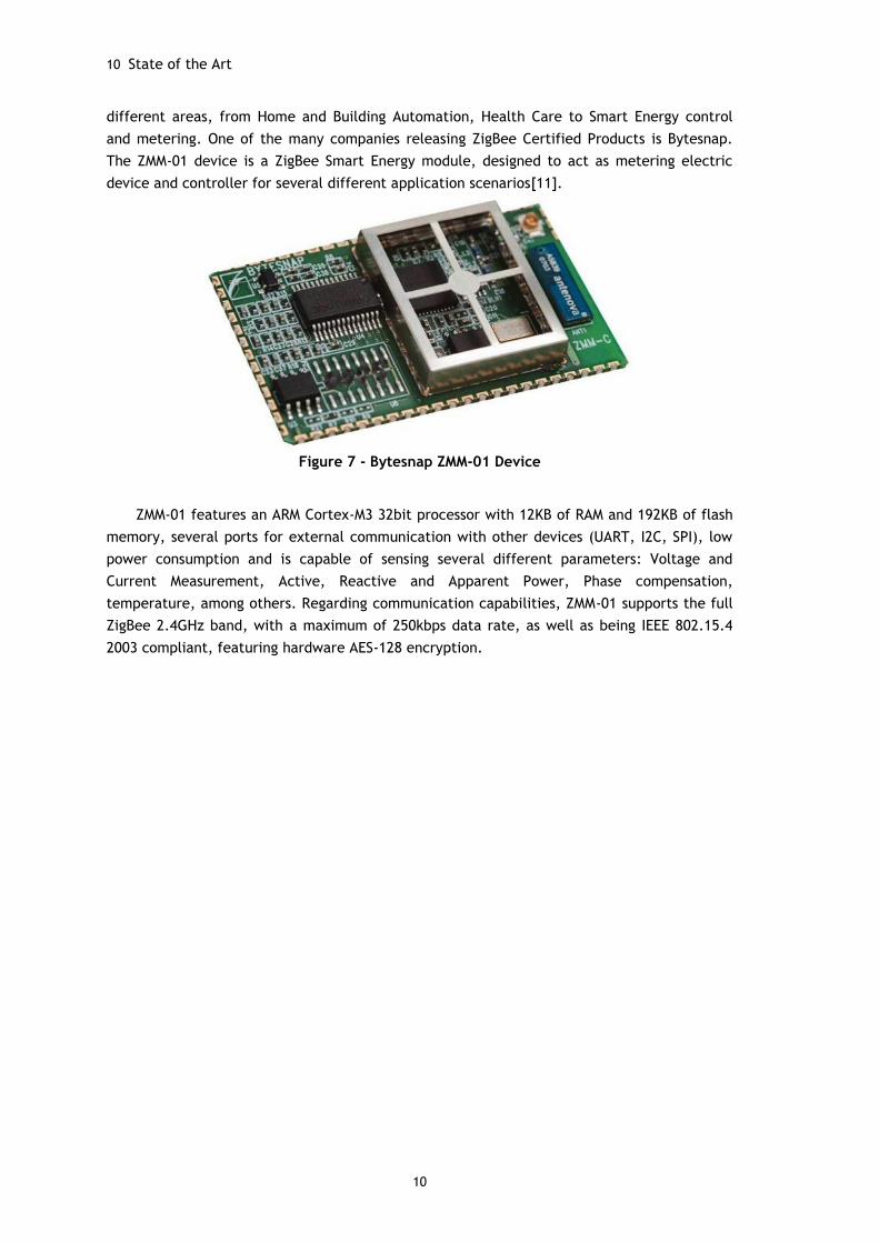
Figure 7 - Bytesnap ZMM-01 Device
ZMM-01 features an ARM Cortex-M3 32bit processor with 12KB of RAM and 192KB of flash
memory, several ports for external communication with other devices (UART, I2C, SPI), low
power consumption and is capable of sensing several different parameters: Voltage and
Current Measurement, Active, Reactive and Apparent Power, Phase compensation,
temperature, among others. Regarding communication capabilities, ZMM-01 supports the full
ZigBee 2.4GHz band, with a maximum of 250kbps data rate, as well as being IEEE 802.15.4
2003 compliant, featuring hardware AES-128 encryption.
Technologies research 11
11
2.2 Technologies research
In this chapter the technologies behind the solutions addressed in the previous chapter
will be described in more detail. IEEE 802.15.4, 6LoWPAN and RPL Routing Protocol are
technologies relevant to the Contiki solution, while IEEE 802.11 refers to the low-power WiFi
solutions. Other technologies such as ZigBee will also be described, although with less detail.
2.2.1 IEEE 802.15.4-2006
IEEE 802.15.4 is a standard defined by IEEE especially designed to operate on Low Rate
Wireless Personal Area Networks. It focuses on providing low cost, short-range, low power
and low speed communication for a ubiquitous sensor network. IEEE 802.15.4 defines both
the PHY and MAC layers according to the OSI model, while the upper layers are out of scope
for this standard, being defined by other architectures such as ZigBee, ISA100.11a,
WirelessHART or MiWi.
The standard defines two different types of nodes: a full-function device (FFD) and a
reduced-function device (RFD)[12]. RFDs are very basic nodes with little processing and
memory resources, therefore only act as end-systems in the network. RFDs don't implement
many of the standard functionalities, being able to communicate only to FFDs. FFDs are
devices with more capabilities and are able to fully implement the standard. FFDs can
communicate with both FFDs and RFDs and can act as coordinators (PAN or full network
coordinators).
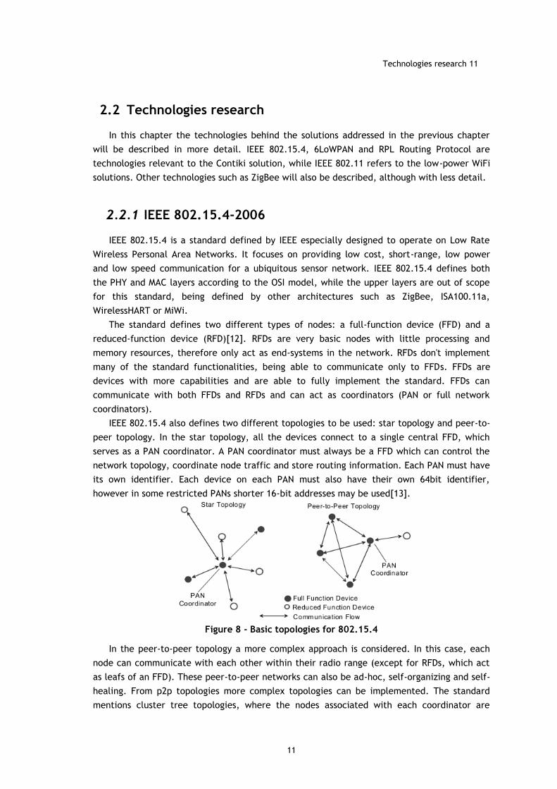
IEEE 802.15.4 also defines two different topologies to be used: star topology and peer-to-
peer topology. In the star topology, all the devices connect to a single central FFD, which
serves as a PAN coordinator. A PAN coordinator must always be a FFD which can control the
network topology, coordinate node traffic and store routing information. Each PAN must have
its own identifier. Each device on each PAN must also have their own 64bit identifier,
however in some restricted PANs shorter 16-bit addresses may be used[13].
Figure 8 - Basic topologies for 802.15.4
In the peer-to-peer topology a more complex approach is considered. In this case, each
node can communicate with each other within their radio range (except for RFDs, which act
as leafs of an FFD). These peer-to-peer networks can also be ad-hoc, self-organizing and self-
healing. From p2p topologies more complex topologies can be implemented. The standard
mentions cluster tree topologies, where the nodes associated with each coordinator are
12 State of the Art
12
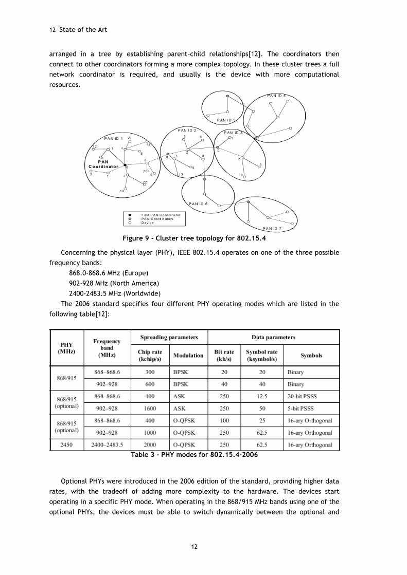
arranged in a tree by establishing parent-child relationships[12]. The coordinators then
connect to other coordinators forming a more complex topology. In these cluster trees a full
network coordinator is required, and usually is the device with more computational
resources.
Figure 9 - Cluster tree topology for 802.15.4
Concerning the physical layer (PHY), IEEE 802.15.4 operates on one of the three possible
frequency bands:
868.0-868.6 MHz (Europe)
902-928 MHz (North America)
2400-2483.5 MHz (Worldwide)
The 2006 standard specifies four different PHY operating modes which are listed in the
following table[12]:
Table 3 - PHY modes for 802.15.4-2006
Optional PHYs were introduced in the 2006 edition of the standard, providing higher data
rates, with the tradeoff of adding more complexity to the hardware. The devices start
operating in a specific PHY mode. When operating in the 868/915 MHz bands using one of the
optional PHYs, the devices must be able to switch dynamically between the optional and
Technologies research 13
13
regular operating modes. Furthermore, standard revisions 4a, 4c and 4d were released with
several additional PHY operating modes and frequencies [14-16].
The MAC sublayer provides both MAC Data and MAC Management services, with features
such as channel access, association and dissociation of the nodes in the PAN, beacon and
Guaranteed Time Slot (GTS) management, frame validation and acknowledgment. The MAC
sublayer also provides the upper layers with tools to provide security mechanisms, such as
AES-128.
The standard supports two operation modes, namely the beacon-enabled mode and the
non-beacon enabled mode. The first uses the superframe structure, which can have both
active and inactive portions. The superframe is bounded by beacons, sent by the PAN
coordinator in order to synchronize the network nodes and define the superframe structure.
The active portion of the superframe may be divided in Contention Access Period (CAP) and
Contention Free Period (CFP). In the CAP the devices use a slotted CSMA/CA algorithm to gain
access to the channel, while in the CFP there are GTS for the devices to use. CFP is used by
devices with specific bandwidth and latency requirements. The inactive portion of the
superframe is a measure to enable the nodes to enter a coordinated power-saving mode. The
non-beacon enabled mode is entirely based on contention access, using unslotted CSMA/CA
algorithms to gain channel access[12, 17].
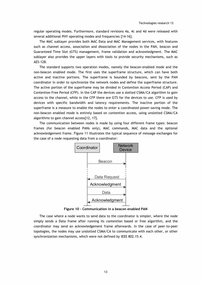
The communication between nodes is made by using four different frame types: beacon
frames (for beacon enabled PANs only), MAC commands, MAC data and the optional
acknowledgement frame. Figure 11 illustrates the typical sequence of message exchanges for
the case of a node requesting data from a coordinator:
Figure 10 - Communication in a beacon enabled PAN
The case where a node wants to send data to the coordinator is simpler, where the node
simply sends a Data frame after running its contention based or free algorithm, and the
coordinator may send an acknowledgement frame afterwards. In the case of peer-to-peer
topologies, the nodes may use unslotted CSMA/CA to communicate with each other, or other
synchronization mechanisms, which were not defined by IEEE 802.15.4.
14 State of the Art
14
2.2.2 6LoWPAN
6LoWPAN is a standard defined by IETF which infers to IPv6 over Low power Wireless
Personal Area Networks. It was developed to adapt IPv6 communication on top of IEEE
802.15.4 networks. The IPv6 protocol is the successor of the older IPv4 protocol and while it
was primarily developed to solve the inevitable IPv4 address exhaustion (IPv6 has a 128bit
address range as opposed to IPv4’s 32bit), it introduced several new features and redesigns.
IPv6 was developed in the context of high powered devices and capable networks. However,
the IEEE 802.15.4 is the total opposite, operating on LLNs with very low powered and
constrained devices. Integrating all the IPv6 features on such constrained networks
represents a formidable challenge that is still currently being addressed by the IETF
workgroup 6lowpan. 6lowpan already released three RFCs defining the 6LoWPAN protocol,
and 4 more drafts are being developed to extend the 6LoWPAN capabilities, such as
implementing adapting IPv6 Neighbor Discovery mechanisms, or even adapting 6LoWPAN to
Bluetooth networks.
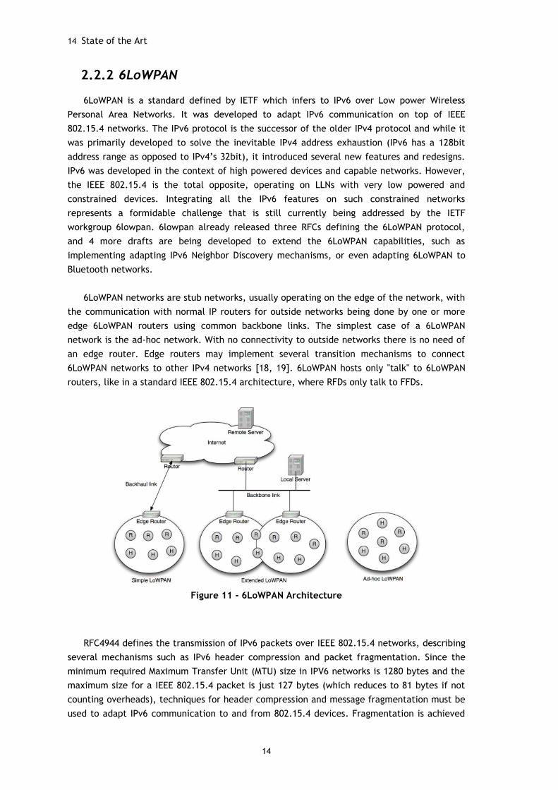
6LoWPAN networks are stub networks, usually operating on the edge of the network, with
the communication with normal IP routers for outside networks being done by one or more
edge 6LoWPAN routers using common backbone links. The simplest case of a 6LoWPAN
network is the ad-hoc network. With no connectivity to outside networks there is no need of
an edge router. Edge routers may implement several transition mechanisms to connect
6LoWPAN networks to other IPv4 networks [18, 19]. 6LoWPAN hosts only "talk" to 6LoWPAN
routers, like in a standard IEEE 802.15.4 architecture, where RFDs only talk to FFDs.
Figure 11 - 6LoWPAN Architecture
RFC4944 defines the transmission of IPv6 packets over IEEE 802.15.4 networks, describing
several mechanisms such as IPv6 header compression and packet fragmentation. Since the
minimum required Maximum Transfer Unit (MTU) size in IPV6 networks is 1280 bytes and the
maximum size for a IEEE 802.15.4 packet is just 127 bytes (which reduces to 81 bytes if not
counting overheads), techniques for header compression and message fragmentation must be
used to adapt IPv6 communication to and from 802.15.4 devices. Fragmentation is achieved
Technologies research 15
15
with the inclusion of a fragmentation subheader in the messages, including fields such as
Datagram Tag and Datagram offset, which are used to identify the set of unfragmented
payload the fragments belong, or the offset of the fragmented packet within the
unfragmented payload, respectively. Even if 6LoWPAN has message fragmentation
mechanisms, the applications should not allow the transmission of big packets that require
fragmentation, due to performance issues. Since the target environment of operation are
lossy networks, the loss of a fragment means the retransmission of the full packet[19].
The addresses in IPv6 consist of a 64 bit prefix, which is common to all the devices in the
network, and a 64 bit Interface ID. RFC4994 introduced the concept of IPv6 header
compression (HC1) and UDP header compression (HC2). Regarding the address compression,
the prefix is known to all the devices and therefore is elided, and the IDs are also elided for
link-local communication. A standard UDP/IPv6 header is 48 bytes long, using both HC1 and
HC2 mechanisms the header is compressed to only ~7 bytes, considering the simplest case
where a datagram is sent inside the PAN, using the 16-bit addresses. However, outside of the
unicast link-local scope the HC1 and HC2 mechanisms do not efficiently compress the
headers. In a link-local multicast IPv6 header the full destination address must be included,
bringing down a ~23 bytes long header in the best case. When communicating with an outside
node, the header must include the source prefix and the full destination address, resulting in
a ~31 bytes long header[20].
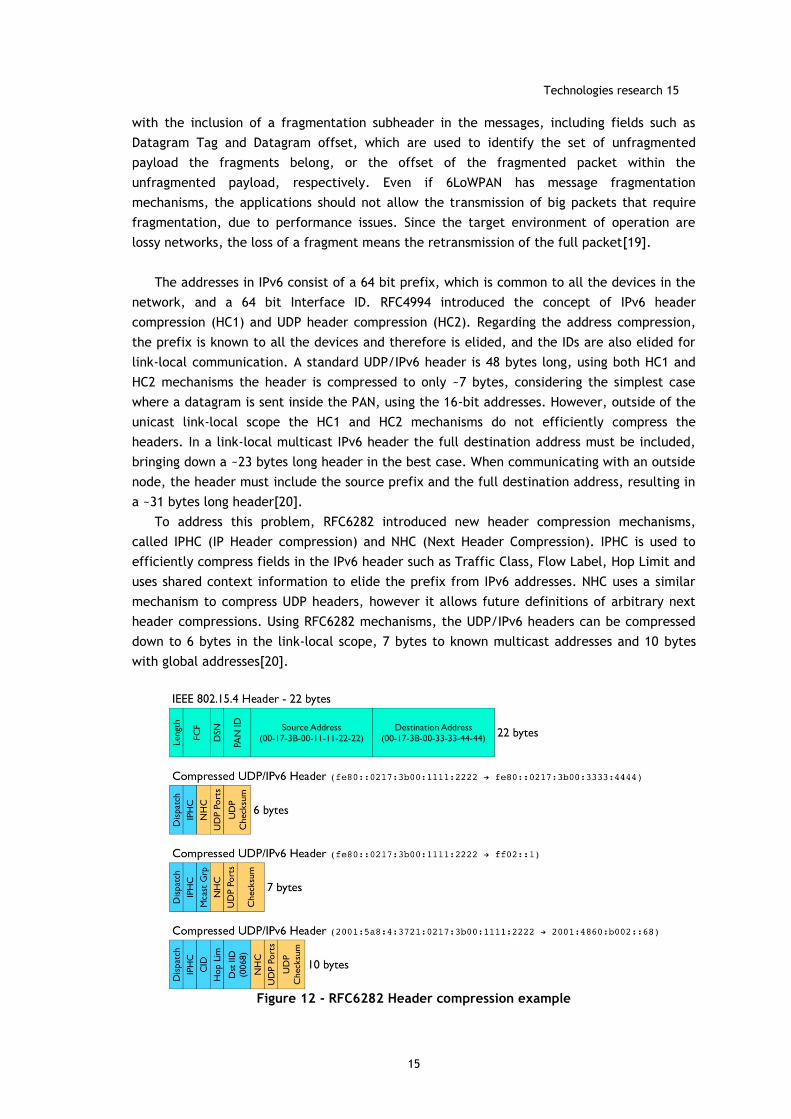
To address this problem, RFC6282 introduced new header compression mechanisms,
called IPHC (IP Header compression) and NHC (Next Header Compression). IPHC is used to
efficiently compress fields in the IPv6 header such as Traffic Class, Flow Label, Hop Limit and
uses shared context information to elide the prefix from IPv6 addresses. NHC uses a similar
mechanism to compress UDP headers, however it allows future definitions of arbitrary next
header compressions. Using RFC6282 mechanisms, the UDP/IPv6 headers can be compressed
down to 6 bytes in the link-local scope, 7 bytes to known multicast addresses and 10 bytes
with global addresses[20].
Figure 12 - RFC6282 Header compression example
16 State of the Art
16
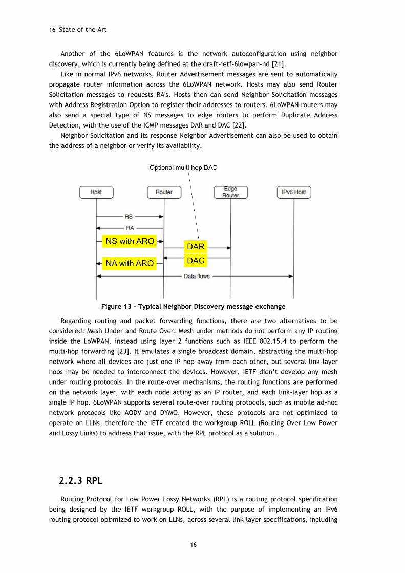
Another of the 6LoWPAN features is the network autoconfiguration using neighbor
discovery, which is currently being defined at the draft-ietf-6lowpan-nd [21].
Like in normal IPv6 networks, Router Advertisement messages are sent to automatically
propagate router information across the 6LoWPAN network. Hosts may also send Router
Solicitation messages to requests RA's. Hosts then can send Neighbor Solicitation messages
with Address Registration Option to register their addresses to routers. 6LoWPAN routers may
also send a special type of NS messages to edge routers to perform Duplicate Address
Detection, with the use of the ICMP messages DAR and DAC [22].
Neighbor Solicitation and its response Neighbor Advertisement can also be used to obtain
the address of a neighbor or verify its availability.
Figure 13 - Typical Neighbor Discovery message exchange
Regarding routing and packet forwarding functions, there are two alternatives to be
considered: Mesh Under and Route Over. Mesh under methods do not perform any IP routing
inside the LoWPAN, instead using layer 2 functions such as IEEE 802.15.4 to perform the
multi-hop forwarding [23]. It emulates a single broadcast domain, abstracting the multi-hop
network where all devices are just one IP hop away from each other, but several link-layer
hops may be needed to interconnect the devices. However, IETF didn’t develop any mesh
under routing protocols. In the route-over mechanisms, the routing functions are performed
on the network layer, with each node acting as an IP router, and each link-layer hop as a
single IP hop. 6LoWPAN supports several route-over routing protocols, such as mobile ad-hoc
network protocols like AODV and DYMO. However, these protocols are not optimized to
operate on LLNs, therefore the IETF created the workgroup ROLL (Routing Over Low Power
and Lossy Links) to address that issue, with the RPL protocol as a solution.
2.2.3 RPL
Routing Protocol for Low Power Lossy Networks (RPL) is a routing protocol specification
being designed by the IETF workgroup ROLL, with the purpose of implementing an IPv6
routing protocol optimized to work on LLNs, across several link layer specifications, including
Technologies research 17
17
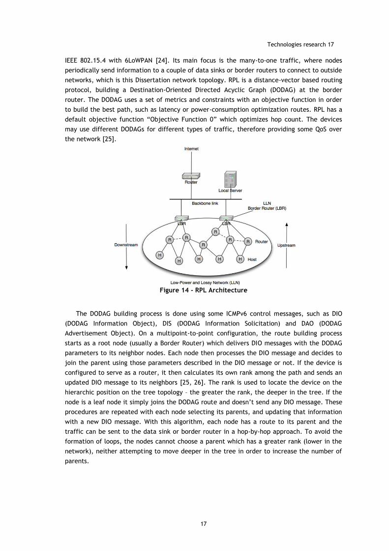
IEEE 802.15.4 with 6LoWPAN [24]. Its main focus is the many-to-one traffic, where nodes
periodically send information to a couple of data sinks or border routers to connect to outside
networks, which is this Dissertation network topology. RPL is a distance-vector based routing
protocol, building a Destination-Oriented Directed Acyclic Graph (DODAG) at the border
router. The DODAG uses a set of metrics and constraints with an objective function in order
to build the best path, such as latency or power-consumption optimization routes. RPL has a
default objective function “Objective Function 0” which optimizes hop count. The devices
may use different DODAGs for different types of traffic, therefore providing some QoS over
the network [25].
Figure 14 - RPL Architecture
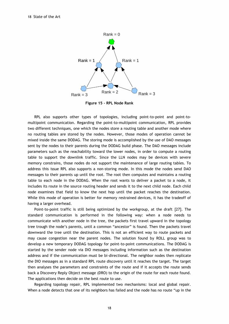
The DODAG building process is done using some ICMPv6 control messages, such as DIO
(DODAG Information Object), DIS (DODAG Information Solicitation) and DAO (DODAG
Advertisement Object). On a multipoint-to-point configuration, the route building process
starts as a root node (usually a Border Router) which delivers DIO messages with the DODAG
parameters to its neighbor nodes. Each node then processes the DIO message and decides to
join the parent using those parameters described in the DIO message or not. If the device is
configured to serve as a router, it then calculates its own rank among the path and sends an
updated DIO message to its neighbors [25, 26]. The rank is used to locate the device on the
hierarchic position on the tree topology – the greater the rank, the deeper in the tree. If the
node is a leaf node it simply joins the DODAG route and doesn’t send any DIO message. These
procedures are repeated with each node selecting its parents, and updating that information
with a new DIO message. With this algorithm, each node has a route to its parent and the
traffic can be sent to the data sink or border router in a hop-by-hop approach. To avoid the
formation of loops, the nodes cannot choose a parent which has a greater rank (lower in the
network), neither attempting to move deeper in the tree in order to increase the number of
parents.
18 State of the Art
18
Figure 15 - RPL Node Rank
RPL also supports other types of topologies, including point-to-point and point-to-
multipoint communication. Regarding the point-to-multipoint communication, RPL provides
two different techniques, one which the nodes store a routing table and another mode where
no routing tables are stored by the nodes. However, those modes of operation cannot be
mixed inside the same DODAG. The storing mode is accomplished by the use of DAO messages
sent by the nodes to their parents during the DODAG build phase. The DAO messages include
parameters such as the reachability toward the lower nodes, in order to compute a routing
table to support the downlink traffic. Since the LLN nodes may be devices with severe
memory constrains, those nodes do not support the maintenance of large routing tables. To
address this issue RPL also supports a non-storing mode. In this mode the nodes send DAO
messages to their parents up until the root. The root then computes and maintains a routing
table to each node in the DODAG. When the root wants to deliver a packet to a node, it
includes its route in the source routing header and sends it to the next child node. Each child
node examines that field to know the next hop until the packet reaches the destination.
While this mode of operation is better for memory restrained devices, it has the tradeoff of
having a larger overhead.
Point-to-point traffic is still being optimized by the workgroup, at the draft [27]. The
standard communication is performed in the following way: when a node needs to
communicate with another node in the tree, the packets first travel upward in the topology
tree trough the node’s parents, until a common “ancestor” is found. Then the packets travel
downward the tree until the destination. This is not an efficient way to route packets and
may cause congestion near the parent nodes. The solution found by ROLL group was to
develop a new temporary DODAG topology for point-to-point communications. The DODAG is
started by the sender node via DIO messages including information such as the destination
address and if the communication must be bi-directional. The neighbor nodes then replicate
the DIO messages as in a standard RPL route discovery until it reaches the target. The target
then analyses the parameters and constraints of the route and if it accepts the route sends
back a Discovery Reply Object message (DRO) to the origin of the route for each route found.
The applications then decide on the best route to use.
Regarding topology repair, RPL implemented two mechanisms: local and global repair.
When a node detects that one of its neighbors has failed and the node has no route “up in the
Technologies research 19
19
tree”, a local repair is executed on that node to find an alternate route, with no implications
to the global topology. However, successive local repairs may lead to a non-efficient tree
topology, and the root may perform a global repair, reshaping the entire tree [25].
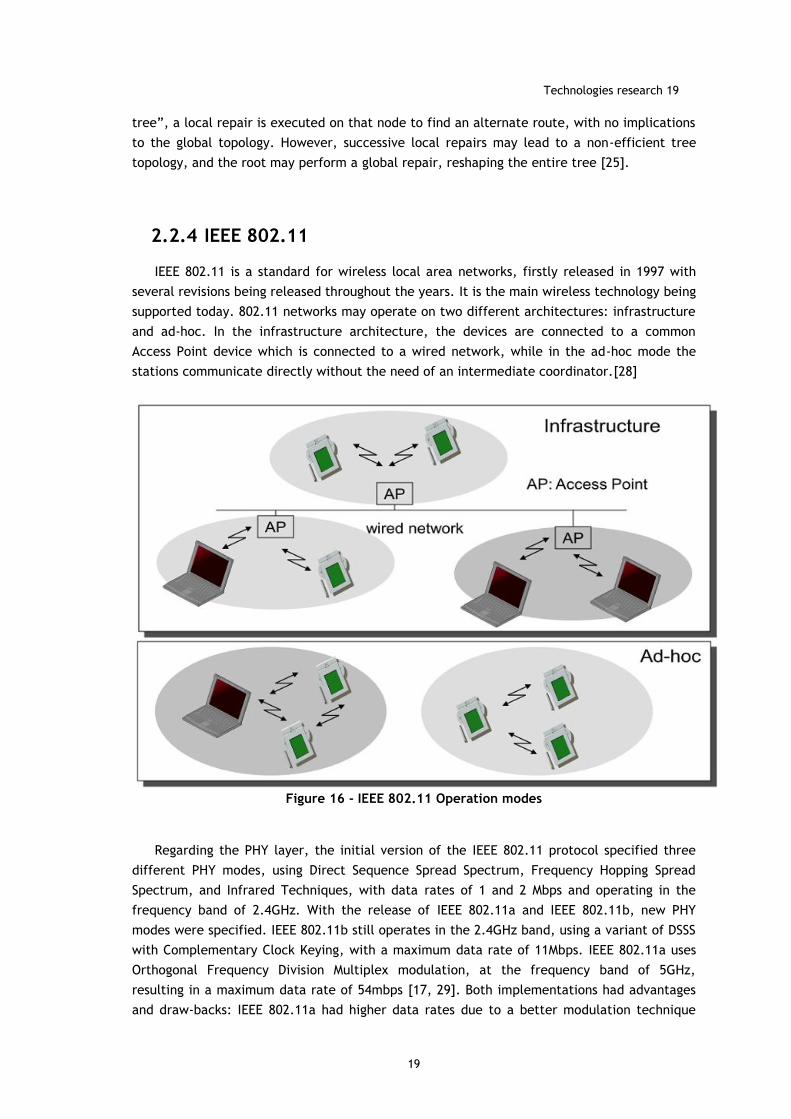
2.2.4 IEEE 802.11
IEEE 802.11 is a standard for wireless local area networks, firstly released in 1997 with
several revisions being released throughout the years. It is the main wireless technology being
supported today. 802.11 networks may operate on two different architectures: infrastructure
and ad-hoc. In the infrastructure architecture, the devices are connected to a common
Access Point device which is connected to a wired network, while in the ad-hoc mode the
stations communicate directly without the need of an intermediate coordinator.[28]
Figure 16 - IEEE 802.11 Operation modes
Regarding the PHY layer, the initial version of the IEEE 802.11 protocol specified three
different PHY modes, using Direct Sequence Spread Spectrum, Frequency Hopping Spread
Spectrum, and Infrared Techniques, with data rates of 1 and 2 Mbps and operating in the
frequency band of 2.4GHz. With the release of IEEE 802.11a and IEEE 802.11b, new PHY
modes were specified. IEEE 802.11b still operates in the 2.4GHz band, using a variant of DSSS
with Complementary Clock Keying, with a maximum data rate of 11Mbps. IEEE 802.11a uses
Orthogonal Frequency Division Multiplex modulation, at the frequency band of 5GHz,
resulting in a maximum data rate of 54mbps [17, 29]. Both implementations had advantages
and draw-backs: IEEE 802.11a had higher data rates due to a better modulation technique
20 State of the Art
20
and operating on a higher frequency band, however IEEE 802.11b had higher transmission
ranges. IEEE 802.11g was the next specification, which also works in the 2.4GHz band and is
able to use the modulation techniques of IEEE 802.11a, having a maximum data rate of
54Mbps, besides being compatible with the older IEEE 802.11b devices. While the theoretical
maximum data rate is the same of IEEE 802.11a, IEEE 802.11b and g devices suffer from
interference from other devices operating in the same 2.4 GHz band, such as Bluetooth and
IEEE 802.15.4 devices, cordless phones or even microwave ovens, which degrades the
performance [30]. Another disadvantage is that in the 2.4GHz band there are 3 non
overlapping channels of 20/22MHz to be used (IEEE 802.11g/b), while in the 5GHz band there
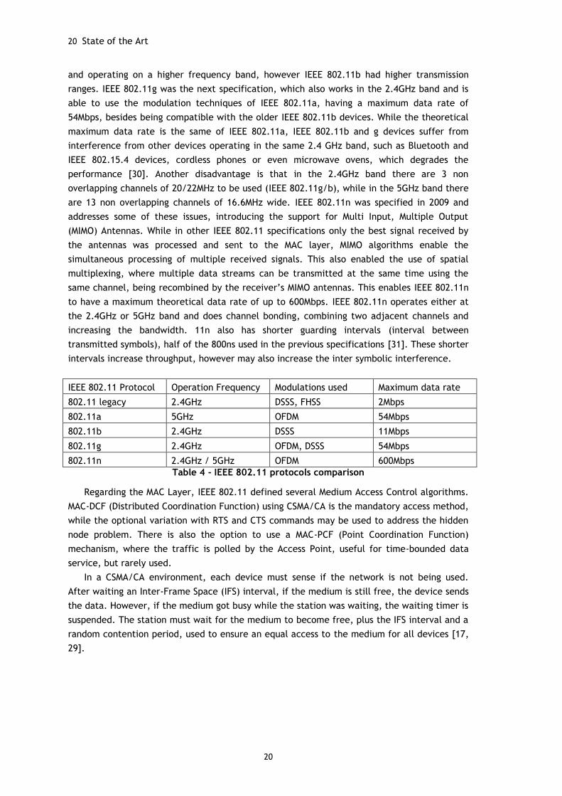
are 13 non overlapping channels of 16.6MHz wide. IEEE 802.11n was specified in 2009 and
addresses some of these issues, introducing the support for Multi Input, Multiple Output
(MIMO) Antennas. While in other IEEE 802.11 specifications only the best signal received by
the antennas was processed and sent to the MAC layer, MIMO algorithms enable the
simultaneous processing of multiple received signals. This also enabled the use of spatial
multiplexing, where multiple data streams can be transmitted at the same time using the
same channel, being recombined by the receiver’s MIMO antennas. This enables IEEE 802.11n
to have a maximum theoretical data rate of up to 600Mbps. IEEE 802.11n operates either at
the 2.4GHz or 5GHz band and does channel bonding, combining two adjacent channels and
increasing the bandwidth. 11n also has shorter guarding intervals (interval between
transmitted symbols), half of the 800ns used in the previous specifications [31]. These shorter
intervals increase throughput, however may also increase the inter symbolic interference.
IEEE 802.11 Protocol Operation Frequency Modulations used Maximum data rate
802.11 legacy 2.4GHz DSSS, FHSS 2Mbps
802.11a 5GHz OFDM 54Mbps
802.11b 2.4GHz DSSS 11Mbps
802.11g 2.4GHz OFDM, DSSS 54Mbps
802.11n 2.4GHz / 5GHz OFDM 600Mbps
Table 4 - IEEE 802.11 protocols comparison
Regarding the MAC Layer, IEEE 802.11 defined several Medium Access Control algorithms.
MAC-DCF (Distributed Coordination Function) using CSMA/CA is the mandatory access method,
while the optional variation with RTS and CTS commands may be used to address the hidden
node problem. There is also the option to use a MAC-PCF (Point Coordination Function)
mechanism, where the traffic is polled by the Access Point, useful for time-bounded data
service, but rarely used.
In a CSMA/CA environment, each device must sense if the network is not being used.
After waiting an Inter-Frame Space (IFS) interval, if the medium is still free, the device sends
the data. However, if the medium got busy while the station was waiting, the waiting timer is
suspended. The station must wait for the medium to become free, plus the IFS interval and a
random contention period, used to ensure an equal access to the medium for all devices [17,
29].
Technologies research 21
21
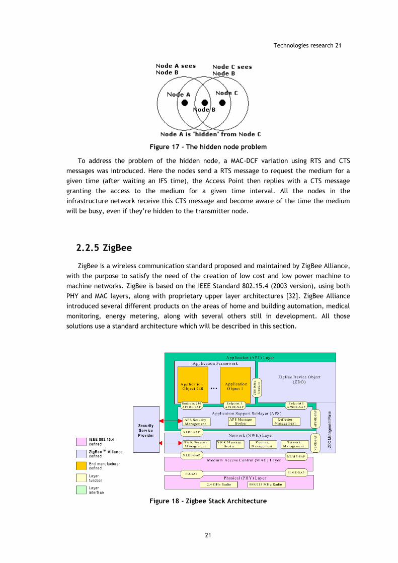
Figure 17 - The hidden node problem
To address the problem of the hidden node, a MAC-DCF variation using RTS and CTS
messages was introduced. Here the nodes send a RTS message to request the medium for a
given time (after waiting an IFS time), the Access Point then replies with a CTS message
granting the access to the medium for a given time interval. All the nodes in the
infrastructure network receive this CTS message and become aware of the time the medium
will be busy, even if they’re hidden to the transmitter node.
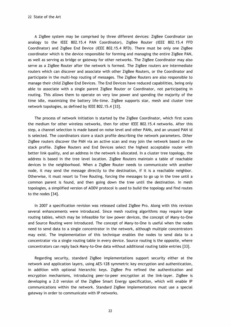
2.2.5 ZigBee
ZigBee is a wireless communication standard proposed and maintained by ZigBee Alliance,
with the purpose to satisfy the need of the creation of low cost and low power machine to
machine networks. ZigBee is based on the IEEE Standard 802.15.4 (2003 version), using both
PHY and MAC layers, along with proprietary upper layer architectures [32]. ZigBee Alliance
introduced several different products on the areas of home and building automation, medical
monitoring, energy metering, along with several others still in development. All those
solutions use a standard architecture which will be described in this section.
Figure 18 - Zigbee Stack Architecture
22 State of the Art
22
A ZigBee system may be comprised by three different devices: ZigBee Coordinator (an
analogy to the IEEE 802.15.4 PAN Coordinator), ZigBee Router (IEEE 802.15.4 FFD
Coordinator) and ZigBee End Device (IEEE 802.15.4 RFD). There must be only one ZigBee
coordinator which is the device responsible for forming and managing the entire ZigBee PAN,
as well as serving as bridge or gateway for other networks. The ZigBee Coordinator may also
serve as a ZigBee Router after the network is formed. The ZigBee routers are intermediate
routers which can discover and associate with other ZigBee Routers, or the Coordinator and
participate in the multi-hop routing of messages. The ZigBee Routers are also responsible to
manage their child ZigBee End Devices. The End Devices have reduced capabilities, being only
able to associate with a single parent ZigBee Router or Coordinator, not participating in
routing. This allows them to operate on very low power and spending the majority of the
time idle, maximizing the battery life-time. ZigBee supports star, mesh and cluster tree
network topologies, as defined by IEEE 802.15.4 [33].
The process of network initiation is started by the ZigBee Coordinator, which first scans
the medium for other wireless networks, then for other IEEE 802.15.4 networks. After this
step, a channel selection is made based on noise level and other PANs, and an unused PAN id
is selected. The coordinators store a stack profile describing the network parameters. Other
ZigBee routers discover the PAN via an active scan and may join the network based on the
stack profile. ZigBee Routers and End Devices select the highest acceptable router with
better link quality, and an address in the network is allocated. In a cluster tree topology, the
address is based in the tree level location. ZigBee Routers maintain a table of reachable
devices in the neighborhood. When a ZigBee Router needs to communicate with another
node, it may send the message directly to the destination, if it is a reachable neighbor.
Otherwise, it must resort to Tree Routing, forcing the messages to go up in the tree until a
common parent is found, and then going down the tree until the destination. In mesh
topologies, a simplified version of AODV protocol is used to build the topology and find routes
to the nodes [34].
In 2007 a specification revision was released called ZigBee Pro. Along with this revision
several enhancements were introduced. Since mesh routing algorithms may require large
routing tables, which may be infeasible for low power devices, the concept of Many-to-One
and Source Routing were introduced. The concept of Many-to-One is useful when the nodes
need to send data to a single concentrator in the network, although multiple concentrators
may exist. The implementation of this technique enables the nodes to send data to a
concentrator via a single routing table in every device. Source routing is the opposite, where
concentrators can reply back Many-to-One data without additional routing table entries [33].
Regarding security, standard ZigBee implementations support security either at the
network and application layers, using AES-128 symmetric key encryption and authentication,
in addition with optional hierarchic keys. ZigBee Pro refined the authentication and
encryption mechanisms, introducing peer-to-peer encryption at the link-layer. ZigBee is
developing a 2.0 version of the ZigBee Smart Energy specification, which will enable IP
communications within the network. Standard ZigBee implementations must use a special
gateway in order to communicate with IP networks.
Technologies research 23
23
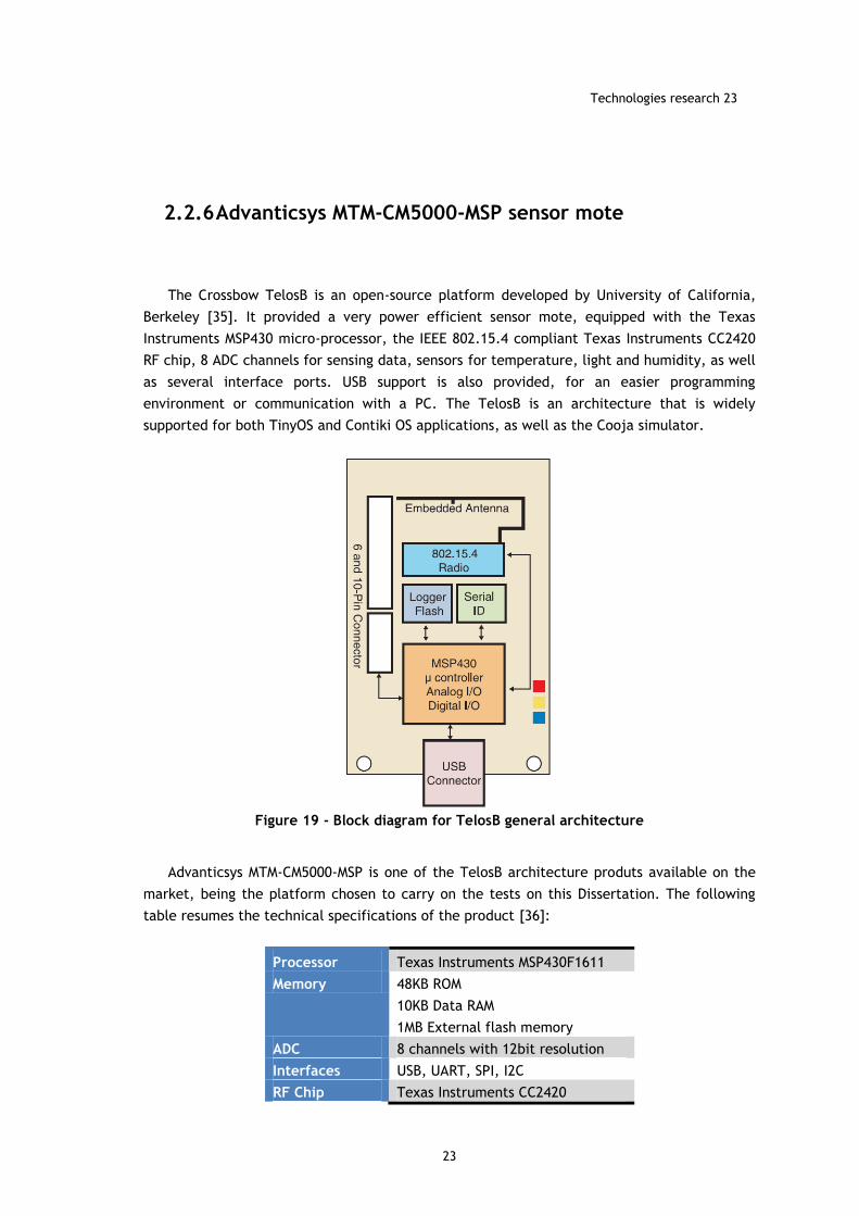
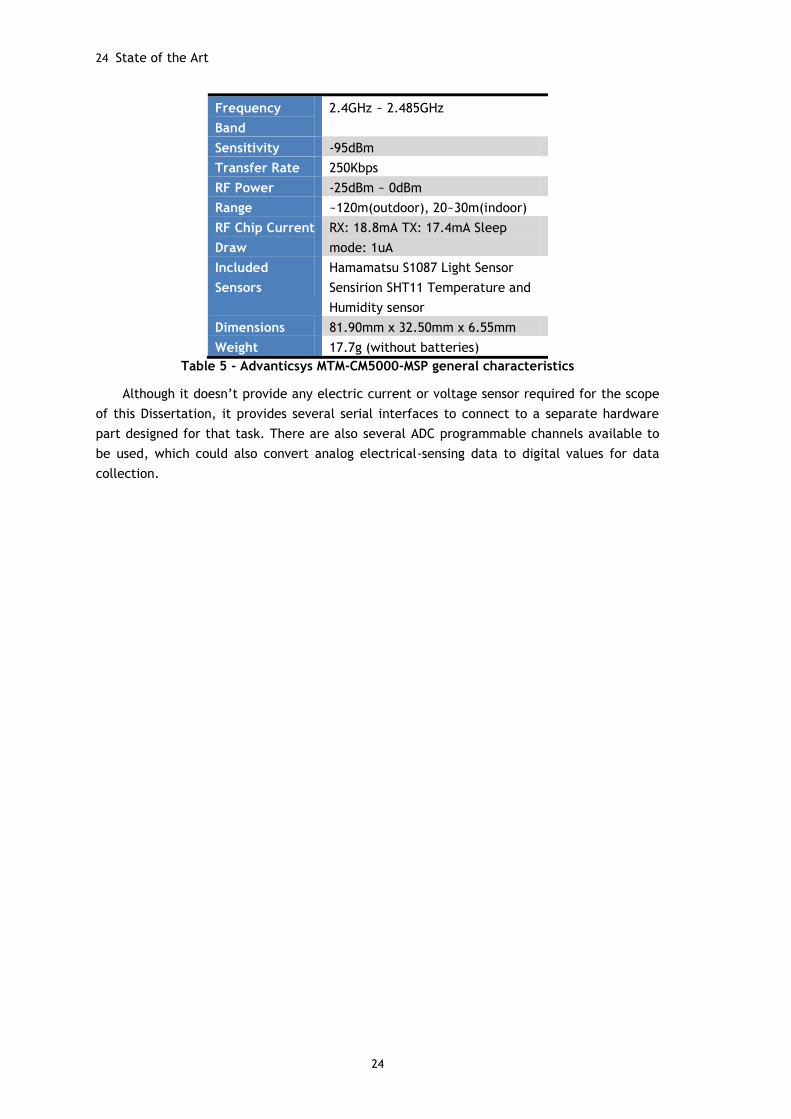
2.2.6 Advanticsys MTM-CM5000-MSP sensor mote
The Crossbow TelosB is an open-source platform developed by University of California,
Berkeley [35]. It provided a very power efficient sensor mote, equipped with the Texas
Instruments MSP430 micro-processor, the IEEE 802.15.4 compliant Texas Instruments CC2420
RF chip, 8 ADC channels for sensing data, sensors for temperature, light and humidity, as well
as several interface ports. USB support is also provided, for an easier programming
environment or communication with a PC. The TelosB is an architecture that is widely
supported for both TinyOS and Contiki OS applications, as well as the Cooja simulator.
Figure 19 - Block diagram for TelosB general architecture
Advanticsys MTM-CM5000-MSP is one of the TelosB architecture produts available on the
market, being the platform chosen to carry on the tests on this Dissertation. The following
table resumes the technical specifications of the product [36]:
Processor Texas Instruments MSP430F1611
Memory 48KB ROM
10KB Data RAM
1MB External flash memory
ADC 8 channels with 12bit resolution
Interfaces USB, UART, SPI, I2C
RF Chip Texas Instruments CC2420
24 State of the Art
24
Frequency
Band
2.4GHz ~ 2.485GHz
Sensitivity -95dBm
Transfer Rate 250Kbps
RF Power -25dBm ~ 0dBm
Range ~120m(outdoor), 20~30m(indoor)
RF Chip Current
Draw
RX: 18.8mA TX: 17.4mA Sleep
mode: 1uA
Included
Sensors
Hamamatsu S1087 Light Sensor
Sensirion SHT11 Temperature and
Humidity sensor
Dimensions 81.90mm x 32.50mm x 6.55mm
Weight 17.7g (without batteries)
Table 5 - Advanticsys MTM-CM5000-MSP general characteristics
Although it doesn’t provide any electric current or voltage sensor required for the scope
of this Dissertation, it provides several serial interfaces to connect to a separate hardware
part designed for that task. There are also several ADC programmable channels available to
be used, which could also convert analog electrical-sensing data to digital values for data
collection.
System description 25
25
Chapter 3
Self-PVP Project
3.1 System Description
As mentioned before, one of the main objectives regarding this dissertation is to validate
the simulation results from Mohammad Abdellatif’s et al SELF-PVP paper [37]. SELF-PVP,
which relates to “Self organizing power management for photo-voltaic power plants”, is a
project concerning the implementation of a large photovoltaic power station, equipped with
smart photovoltaic panels, capable of sensing local variables and communicating among each
other to optimize the general performance of the solar panels arrangement. Mohammad
Abdellatif’s work scope relies in the implementation of a scalable and self-organizing
communication solution for such a large wireless sensor network.
The main system architecture is comprised of a grid network with approximately 200000
solar panels, scattered across an area of 2.5km2, in which each solar panel acts as a node in a
wireless sensor network, having attached a IEEE 802.15.4 compliant sensor for sensing and
communication purposes.
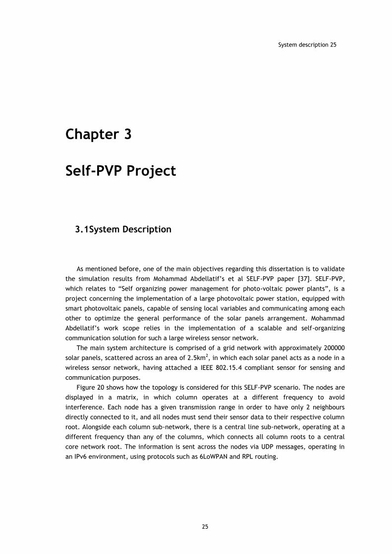
Figure 20 shows how the topology is considered for this SELF-PVP scenario. The nodes are
displayed in a matrix, in which column operates at a different frequency to avoid
interference. Each node has a given transmission range in order to have only 2 neighbours
directly connected to it, and all nodes must send their sensor data to their respective column
root. Alongside each column sub-network, there is a central line sub-network, operating at a
different frequency than any of the columns, which connects all column roots to a central
core network root. The information is sent across the nodes via UDP messages, operating in
an IPv6 environment, using protocols such as 6LoWPAN and RPL routing.
26 Self-PVP Project
26
Figure 20 - System Topology
Three different techniques were presented in Mohammad Abdellatif’s paper to implement
the data collection, with each one being tested 10 times in the Cooja simulator, using
different parameters such as number of nodes in the column and offered load.
Technique 1 consists in having all the nodes in the network to send sensing information
towards the sink node at a constant rate. In Technique 2, the column root nodes send a
broadcast poll to their neighbours, requesting the data. In this case the nodes send the data
towards the root before forwarding the poll to their further neighbour. Technique 3 sends
two different polls for each side of the network, waiting for all the data to be collected from
one side of the network before sending the poll to the other side.
In this dissertation, a small network was initially planned to be deployed in the INESC-
Porto building in order to perform similar tests to validate Mohammad Abdellatif’s
simulations results [37], which will be addressed in the next sections.
Methodology 27
27
3.2 Methodology
The sensors used in the experiments were the Advanticsys MTM-CM5000-MSP motes,
described in the section 2.2.6. The motes are based on the Tmote Sky configuration, and the
Contiki OS 2.5 release was used. The PHY layer used was IEEE 802.15.4, among the nullRDC
MAC layer implementation. This MAC layer implementation enables the nodes to be “awake”
at all time, in order to reduce packet loss and delay in the data transmission process. As in
Mohammad Abdellatif’s SELF-PVP paper, the CSMA-CA mechanism with no acknowledgment
messages was also used in order to avoid unnecessary traffic [37].
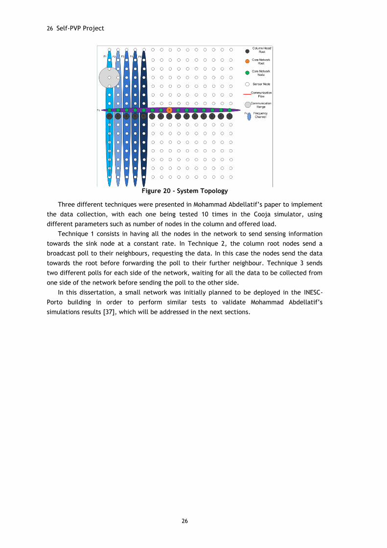
Sink node
Sensor 3
Sensor 4
Sensor 1
Sensor 2
bbbb::212:7400:13b7:6e7e
bbbb::212:7400:13b7:6437
bbbb::212:7400:13b7:7bf2
bbbb::212:7400:13b7:7c91
bbbb::212:7400:13b7:6426
Figure 21 - Network topology
For all Techniques, a network composing of a sink node connected to a linux PC and
several sensor nodes was initially planned to be deployed in INESC-Porto. Mohammad
Abdellatif’s original code was modified in order to be adapted for real-life implementations.
This was necessary because in a Cooja simulation environment all the data regarding each
node in the network can easily be obtained. In a real-life implementation, only the data
“printed” by the sink node can be obtained, or else each other node should also be
connected to a linux PC. The changes in the code will be further explained in the different
Technique sections. As in its original paper, the tests for each Technique were performed 10
times, varying the offered load from 1 packet per second, 2 packets per second and 4 packets
per second. The transport layer protocol used for all Techniques is UDP, due to its
connectionless properties. Figure 21 illustrates the network studied in this chapter.
The parameters evaluated on these tests were the average packet loss and average
throughput for each mote sending sensing data. Delay calculations were possible in a Cooja
simulation environment due to all the information being able to be printed and time stamped
in a Cooja log file. In a real-life scenario, such timestamp information is not possible to
obtain since the motes are not synchronized.
In order to get the information from the sink node, the sink node was programmed with
both the Mohammad Abdellatif’s Techniques source code, but as well as the Serial SHELL
application, which enabled to login to the sink node via an Universal Serial BUS (USB) cable.
With this setup, it is possible to see the information at the sink node being printed in a shell
window. For all the tests in this chapter, the tests were performed using this command:
28 Self-PVP Project
28
make login TARGET=sky | tee logx.txt
The login parameter enables the user to access the information being printed in the shell
by the sink node. The TARGET parameter is just an indication to the makefile in order to set
it to a telosB/sky device, such as the one that is being used in this Dissertation. The tee
parameter is used to save everything that is being printed in the shell window to a given log
file. The x value is changed every test.
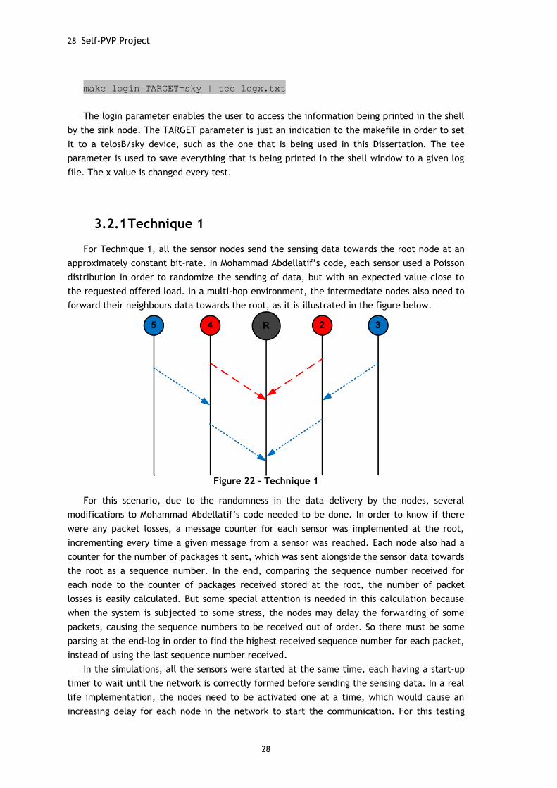
3.2.1 Technique 1
For Technique 1, all the sensor nodes send the sensing data towards the root node at an
approximately constant bit-rate. In Mohammad Abdellatif’s code, each sensor used a Poisson
distribution in order to randomize the sending of data, but with an expected value close to
the requested offered load. In a multi-hop environment, the intermediate nodes also need to
forward their neighbours data towards the root, as it is illustrated in the figure below.
Figure 22 - Technique 1
For this scenario, due to the randomness in the data delivery by the nodes, several
modifications to Mohammad Abdellatif’s code needed to be done. In order to know if there
were any packet losses, a message counter for each sensor was implemented at the root,
incrementing every time a given message from a sensor was reached. Each node also had a
counter for the number of packages it sent, which was sent alongside the sensor data towards
the root as a sequence number. In the end, comparing the sequence number received for
each node to the counter of packages received stored at the root, the number of packet
losses is easily calculated. But some special attention is needed in this calculation because
when the system is subjected to some stress, the nodes may delay the forwarding of some
packets, causing the sequence numbers to be received out of order. So there must be some
parsing at the end-log in order to find the highest received sequence number for each packet,
instead of using the last sequence number received.
In the simulations, all the sensors were started at the same time, each having a start-up
timer to wait until the network is correctly formed before sending the sensing data. In a real
life implementation, the nodes need to be activated one at a time, which would cause an
increasing delay for each node in the network to start the communication. For this testing
Methodology 29
29
scenario, in order to have the sensors to start sending the sensing data at the same time, it
was implemented a special multicast poll in order to trigger that process. Every time the user
button available on the sink node is pressed, the network map is displayed, with the direct
neighbours identified and all the routes to the sensors in the network, the destination node
and the next hop. If the expected number of nodes is already mapped in the routing table,
then the trigger poll is broadcasted. Otherwise, pressing the button wouldn’t trigger this poll,
printing only the routing table information. The poll is broadcasted to all the neighbours, and
each neighbour starts sending their sensing data towards the root before forwarding the poll
to the next hop.
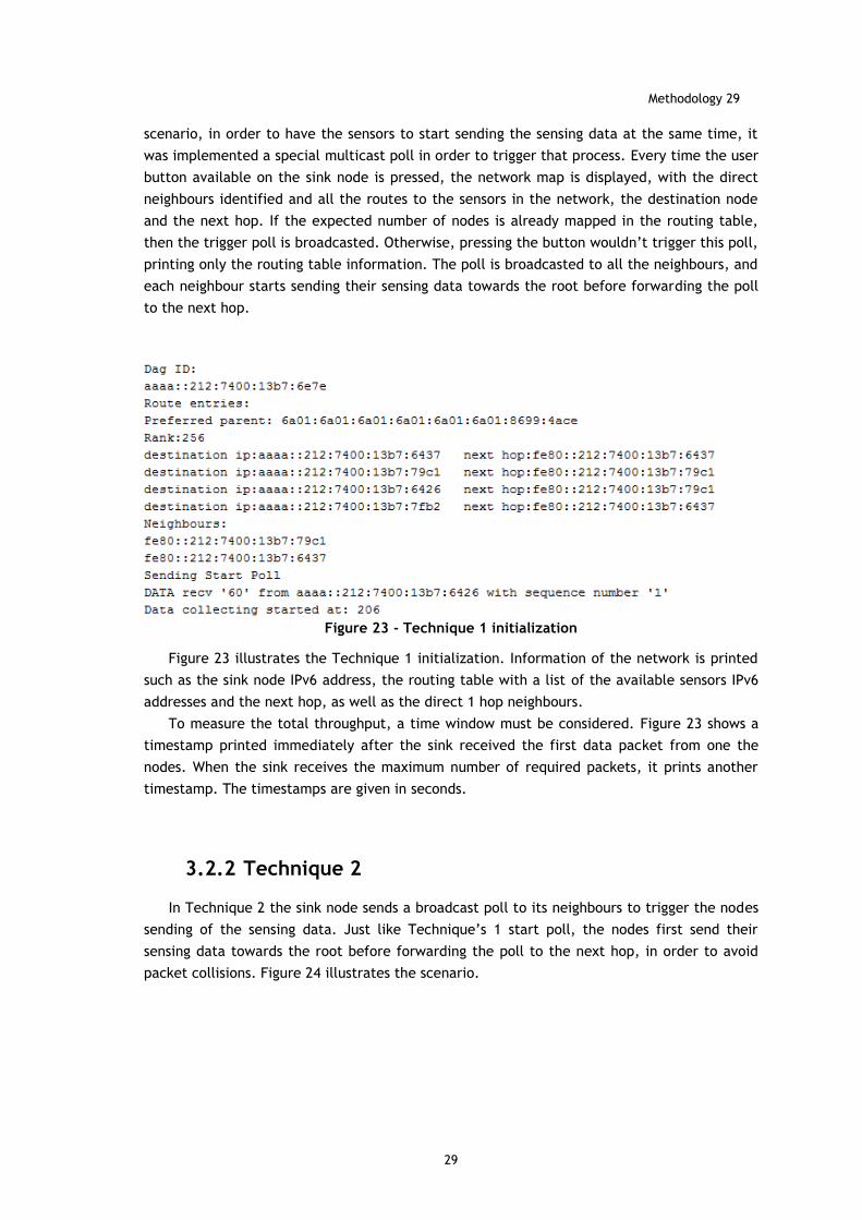
Figure 23 - Technique 1 initialization
Figure 23 illustrates the Technique 1 initialization. Information of the network is printed
such as the sink node IPv6 address, the routing table with a list of the available sensors IPv6
addresses and the next hop, as well as the direct 1 hop neighbours.
To measure the total throughput, a time window must be considered. Figure 23 shows a
timestamp printed immediately after the sink received the first data packet from one the
nodes. When the sink receives the maximum number of required packets, it prints another
timestamp. The timestamps are given in seconds.
3.2.2 Technique 2
In Technique 2 the sink node sends a broadcast poll to its neighbours to trigger the nodes
sending of the sensing data. Just like Technique’s 1 start poll, the nodes first send their
sensing data towards the root before forwarding the poll to the next hop, in order to avoid
packet collisions. Figure 24 illustrates the scenario.
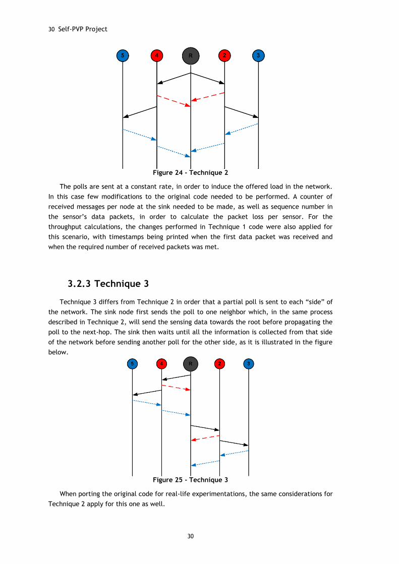
30 Self-PVP Project
30
Figure 24 - Technique 2
The polls are sent at a constant rate, in order to induce the offered load in the network.
In this case few modifications to the original code needed to be performed. A counter of
received messages per node at the sink needed to be made, as well as sequence number in
the sensor’s data packets, in order to calculate the packet loss per sensor. For the
throughput calculations, the changes performed in Technique 1 code were also applied for
this scenario, with timestamps being printed when the first data packet was received and
when the required number of received packets was met.
3.2.3 Technique 3
Technique 3 differs from Technique 2 in order that a partial poll is sent to each “side” of
the network. The sink node first sends the poll to one neighbor which, in the same process
described in Technique 2, will send the sensing data towards the root before propagating the
poll to the next-hop. The sink then waits until all the information is collected from that side
of the network before sending another poll for the other side, as it is illustrated in the figure
below.
Figure 25 - Technique 3
When porting the original code for real-life experimentations, the same considerations for
Technique 2 apply for this one as well.
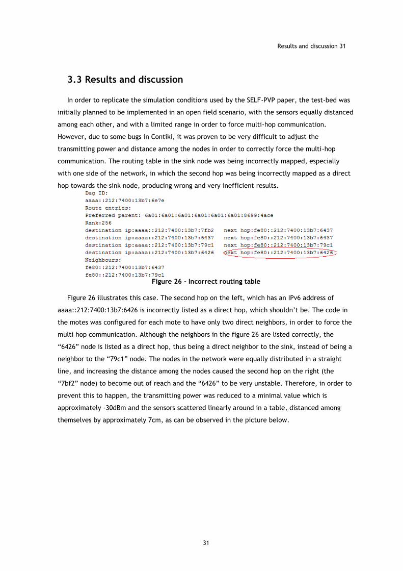
Results and discussion 31
31
3.3 Results and discussion
In order to replicate the simulation conditions used by the SELF-PVP paper, the test-bed was
initially planned to be implemented in an open field scenario, with the sensors equally distanced
among each other, and with a limited range in order to force multi-hop communication.
However, due to some bugs in Contiki, it was proven to be very difficult to adjust the
transmitting power and distance among the nodes in order to correctly force the multi-hop
communication. The routing table in the sink node was being incorrectly mapped, especially
with one side of the network, in which the second hop was being incorrectly mapped as a direct
hop towards the sink node, producing wrong and very inefficient results.
Figure 26 - Incorrect routing table
Figure 26 illustrates this case. The second hop on the left, which has an IPv6 address of
aaaa::212:7400:13b7:6426 is incorrectly listed as a direct hop, which shouldn’t be. The code in
the motes was configured for each mote to have only two direct neighbors, in order to force the
multi hop communication. Although the neighbors in the figure 26 are listed correctly, the
“6426” node is listed as a direct hop, thus being a direct neighbor to the sink, instead of being a
neighbor to the “79c1” node. The nodes in the network were equally distributed in a straight
line, and increasing the distance among the nodes caused the second hop on the right (the
“7bf2” node) to become out of reach and the “6426” to be very unstable. Therefore, in order to
prevent this to happen, the transmitting power was reduced to a minimal value which is
approximately -30dBm and the sensors scattered linearly around in a table, distanced among
themselves by approximately 7cm, as can be observed in the picture below.
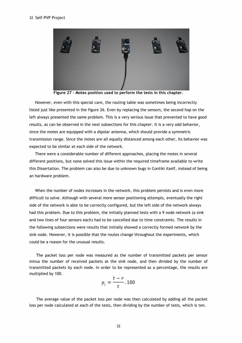
32 Self-PVP Project
32
Figure 27 - Motes position used to perform the tests in this chapter.
However, even with this special care, the routing table was sometimes being incorrectly
listed just like presented in the figure 26. Even by replacing the sensors, the second hop on the
left always presented the same problem. This is a very serious issue that prevented to have good
results, as can be observed in the next subsections for this chapter. It is a very odd behavior,
since the motes are equipped with a dipolar antenna, which should provide a symmetric
transmission range. Since the motes are all equally distanced among each other, its behavior was
expected to be similar at each side of the network.
There were a considerable number of different approaches, placing the motes in several
different positions, but none solved this issue within the required timeframe available to write
this Dissertation. The problem can also be due to unknown bugs in Contiki itself, instead of being
an hardware problem.
When the number of nodes increases in the network, this problem persists and is even more
difficult to solve. Although with several more sensor positioning attempts, eventually the right
side of the network is able to be correctly configured, but the left side of the network always
had this problem. Due to this problem, the initially planned tests with a 9 node network (a sink
and two lines of four sensors each) had to be cancelled due to time constraints. The results in
the following subsections were results that initially showed a correctly formed network by the
sink node. However, it is possible that the routes change throughout the experiments, which
could be a reason for the unusual results.
The packet loss per node was measured as the number of transmitted packets per sensor
minus the number of received packets at the sink node, and then divided by the number of
transmitted packets by each node. In order to be represented as a percentage, the results are
multiplied by 100.
The average value of the packet loss per node was then calculated by adding all the packet
loss per node calculated at each of the tests, then dividing by the number of tests, which is ten.

Results and discussion 33
33
The throughput per node is calculated by dividing the number of packets received per node
by the test time. The test time was possible to obtain by changing the original sink source codes
to print on the screen a timestamp of when the first data packet from any other mote in the
network arrived, and then another timestamp when the number of received data packets has
reached 4000.
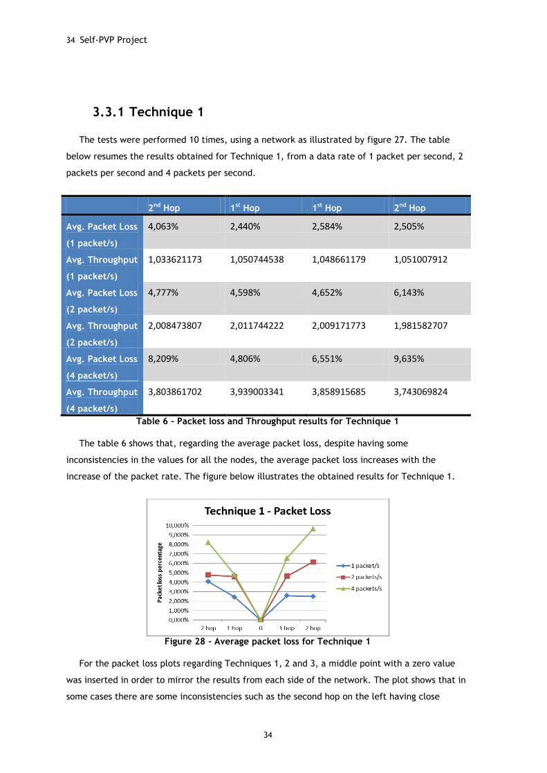
34 Self-PVP Project
34
3.3.1 Technique 1
The tests were performed 10 times, using a network as illustrated by figure 27. The table
below resumes the results obtained for Technique 1, from a data rate of 1 packet per second, 2
packets per second and 4 packets per second.
2nd Hop 1st Hop 1st Hop 2nd Hop
Avg. Packet Loss
(1 packet/s)
4,063% 2,440% 2,584% 2,505%
Avg. Throughput
(1 packet/s)
1,033621173 1,050744538 1,048661179 1,051007912
Avg. Packet Loss
(2 packet/s)
4,777% 4,598% 4,652% 6,143%
Avg. Throughput
(2 packet/s)
2,008473807 2,011744222 2,009171773 1,981582707
Avg. Packet Loss
(4 packet/s)
8,209% 4,806% 6,551% 9,635%
Avg. Throughput
(4 packet/s)
3,803861702 3,939003341 3,858915685 3,743069824
Table 6 - Packet loss and Throughput results for Technique 1
The table 6 shows that, regarding the average packet loss, despite having some
inconsistencies in the values for all the nodes, the average packet loss increases with the
increase of the packet rate. The figure below illustrates the obtained results for Technique 1.
Figure 28 - Average packet loss for Technique 1
For the packet loss plots regarding Techniques 1, 2 and 3, a middle point with a zero value
was inserted in order to mirror the results from each side of the network. The plot shows that in
some cases there are some inconsistencies such as the second hop on the left having close
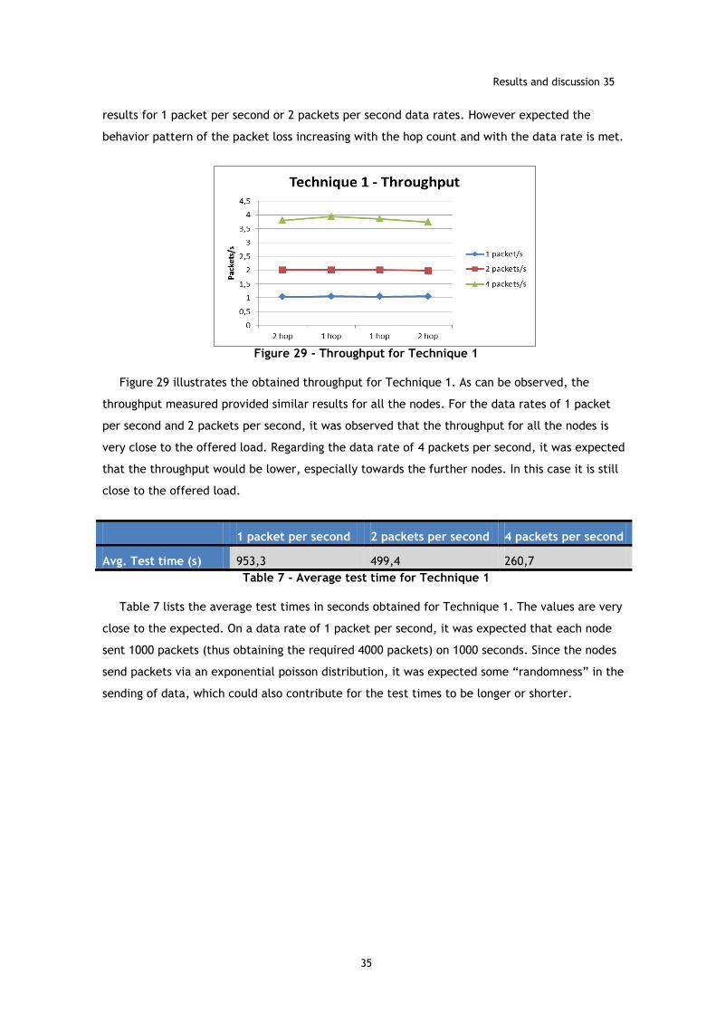
Results and discussion 35
35
results for 1 packet per second or 2 packets per second data rates. However expected the
behavior pattern of the packet loss increasing with the hop count and with the data rate is met.
Figure 29 - Throughput for Technique 1
Figure 29 illustrates the obtained throughput for Technique 1. As can be observed, the
throughput measured provided similar results for all the nodes. For the data rates of 1 packet
per second and 2 packets per second, it was observed that the throughput for all the nodes is
very close to the offered load. Regarding the data rate of 4 packets per second, it was expected
that the throughput would be lower, especially towards the further nodes. In this case it is still
close to the offered load.
1 packet per second 2 packets per second 4 packets per second
Avg. Test time (s) 953,3 499,4 260,7
Table 7 - Average test time for Technique 1
Table 7 lists the average test times in seconds obtained for Technique 1. The values are very
close to the expected. On a data rate of 1 packet per second, it was expected that each node
sent 1000 packets (thus obtaining the required 4000 packets) on 1000 seconds. Since the nodes
send packets via an exponential poisson distribution, it was expected some “randomness” in the
sending of data, which could also contribute for the test times to be longer or shorter.
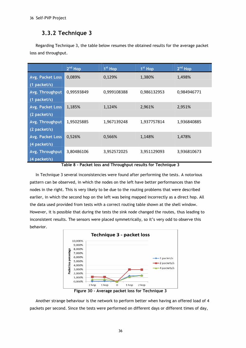
36 Self-PVP Project
36
3.3.2 Technique 3
Regarding Technique 3, the table below resumes the obtained results for the average packet
loss and throughput.
2nd Hop 1st Hop 1st Hop 2nd Hop
Avg. Packet Loss
(1 packet/s)
0,089% 0,129% 1,380% 1,498%
Avg. Throughput
(1 packet/s)
0,99593849 0,999108388 0,986132953 0,984946771
Avg. Packet Loss
(2 packet/s)
1,185% 1,124% 2,961% 2,951%
Avg. Throughput
(2 packet/s)
1,95025885 1,967139248 1,937757814 1,936840885
Avg. Packet Loss
(4 packet/s)
0,526% 0,566% 1,148% 1,478%
Avg. Throughput
(4 packet/s)
3,80486106 3,952572025 3,951129093 3,936810673
Table 8 - Packet loss and Throughput results for Technique 3
In Technique 3 several inconsistencies were found after performing the tests. A notorious
pattern can be observed, in which the nodes on the left have better performances than the
nodes in the right. This is very likely to be due to the routing problems that were described
earlier, in which the second hop on the left was being mapped incorrectly as a direct hop. All
the data used provided from tests with a correct routing table shown at the shell window.
However, it is possible that during the tests the sink node changed the routes, thus leading to
inconsistent results. The sensors were placed symmetrically, so it’s very odd to observe this
behavior.
Figure 30 - Average packet loss for Technique 3
Another strange behaviour is the network to perform better when having an offered load of 4
packets per second. Since the tests were performed on different days or different times of day,
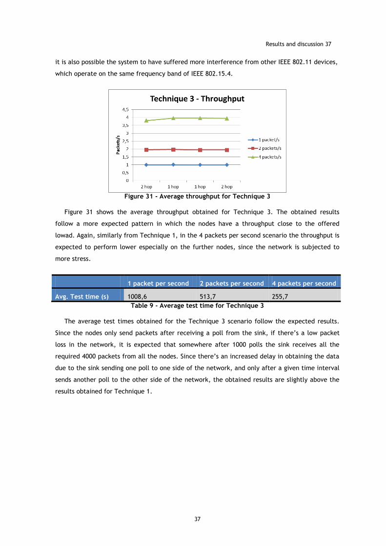
Results and discussion 37
37
it is also possible the system to have suffered more interference from other IEEE 802.11 devices,
which operate on the same frequency band of IEEE 802.15.4.
Figure 31 - Average throughput for Technique 3
Figure 31 shows the average throughput obtained for Technique 3. The obtained results
follow a more expected pattern in which the nodes have a throughput close to the offered
lowad. Again, similarly from Technique 1, in the 4 packets per second scenario the throughput is
expected to perform lower especially on the further nodes, since the network is subjected to
more stress.
1 packet per second 2 packets per second 4 packets per second
Avg. Test time (s) 1008,6 513,7 255,7
Table 9 - Average test time for Technique 3
The average test times obtained for the Technique 3 scenario follow the expected results.
Since the nodes only send packets after receiving a poll from the sink, if there’s a low packet
loss in the network, it is expected that somewhere after 1000 polls the sink receives all the
required 4000 packets from all the nodes. Since there’s an increased delay in obtaining the data
due to the sink sending one poll to one side of the network, and only after a given time interval
sends another poll to the other side of the network, the obtained results are slightly above the
results obtained for Technique 1.
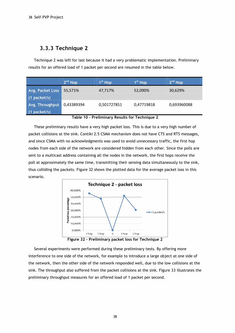
38 Self-PVP Project
38
3.3.3 Technique 2
Technique 2 was left for last because it had a very problematic implementation. Preliminary
results for an offered load of 1 packet per second are resumed in the table below.
2nd Hop 1st Hop 1st Hop 2nd Hop
Avg. Packet Loss
(1 packet/s)
55,571% 47,717% 52,090% 30,629%
Avg. Throughput
(1 packet/s)
0,43389394 0,501727851 0,47719818 0,693960088
Table 10 - Preliminary Results for Technique 2
These preliminary results have a very high packet loss. This is due to a very high number of
packet collisions at the sink. Contiki 2.5 CSMA mechanism does not have CTS and RTS messages,
and since CSMA with no acknowledgments was used to avoid unnecessary traffic, the first hop
nodes from each side of the network are considered hidden from each other. Since the polls are
sent to a multicast address containing all the nodes in the network, the first hops receive the
poll at approximately the same time, transmitting their sensing data simultaneously to the sink,
thus colliding the packets. Figure 32 shows the plotted data for the average packet loss in this
scenario.
Figure 32 - Preliminary packet loss for Technique 2
Several experiments were performed during these preliminary tests. By offering more
interference to one side of the network, for example to introduce a large object at one side of
the network, then the other side of the network responded well, due to the low collisions at the
sink. The throughput also suffered from the packet collisions at the sink. Figure 33 illustrates the
preliminary throughput measures for an offered load of 1 packet per second.
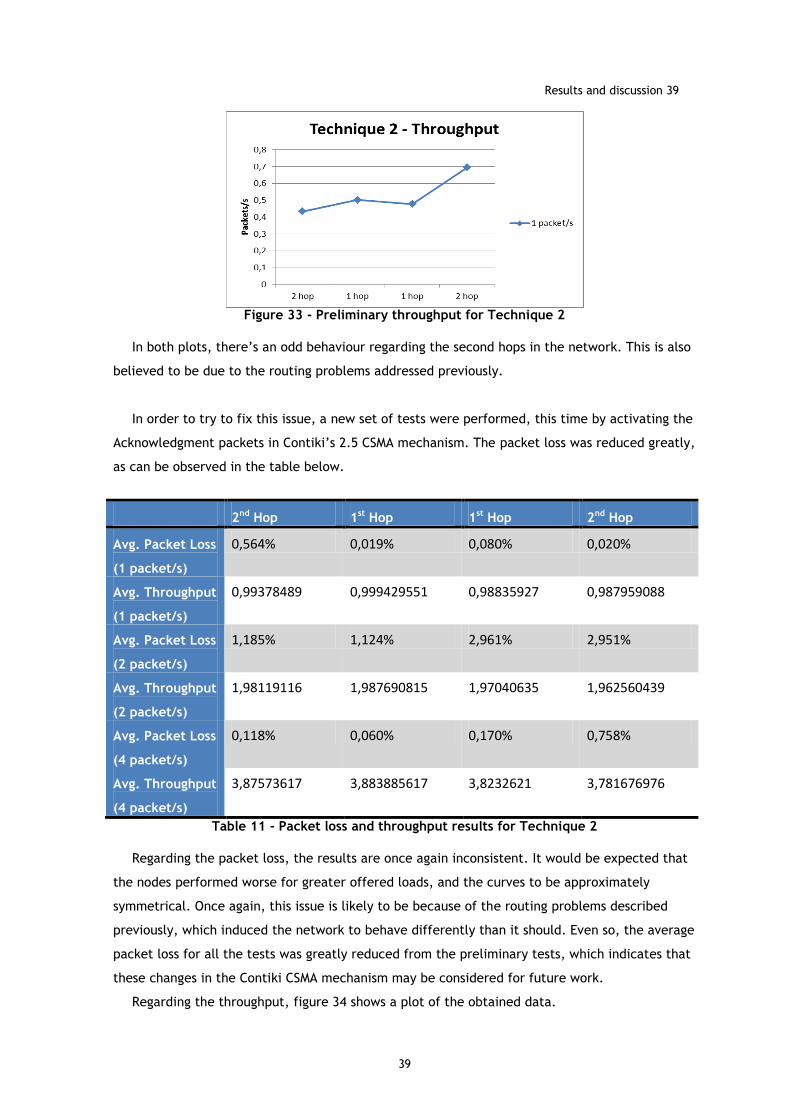
Results and discussion 39
39
Figure 33 - Preliminary throughput for Technique 2
In both plots, there’s an odd behaviour regarding the second hops in the network. This is also
believed to be due to the routing problems addressed previously.
In order to try to fix this issue, a new set of tests were performed, this time by activating the
Acknowledgment packets in Contiki’s 2.5 CSMA mechanism. The packet loss was reduced greatly,
as can be observed in the table below.
2nd Hop 1st Hop 1st Hop 2nd Hop
Avg. Packet Loss
(1 packet/s)
0,564% 0,019% 0,080% 0,020%
Avg. Throughput
(1 packet/s)
0,99378489 0,999429551 0,98835927 0,987959088
Avg. Packet Loss
(2 packet/s)
1,185% 1,124% 2,961% 2,951%
Avg. Throughput
(2 packet/s)
1,98119116 1,987690815 1,97040635 1,962560439
Avg. Packet Loss
(4 packet/s)
0,118% 0,060% 0,170% 0,758%
Avg. Throughput
(4 packet/s)
3,87573617 3,883885617 3,8232621 3,781676976
Table 11 - Packet loss and throughput results for Technique 2
Regarding the packet loss, the results are once again inconsistent. It would be expected that
the nodes performed worse for greater offered loads, and the curves to be approximately
symmetrical. Once again, this issue is likely to be because of the routing problems described
previously, which induced the network to behave differently than it should. Even so, the average
packet loss for all the tests was greatly reduced from the preliminary tests, which indicates that
these changes in the Contiki CSMA mechanism may be considered for future work.
Regarding the throughput, figure 34 shows a plot of the obtained data.
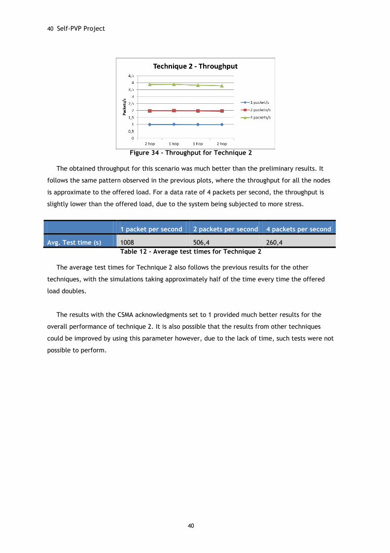
40 Self-PVP Project
40
Figure 34 - Throughput for Technique 2
The obtained throughput for this scenario was much better than the preliminary results. It
follows the same pattern observed in the previous plots, where the throughput for all the nodes
is approximate to the offered load. For a data rate of 4 packets per second, the throughput is
slightly lower than the offered load, due to the system being subjected to more stress.
1 packet per second 2 packets per second 4 packets per second
Avg. Test time (s) 1008 506,4 260,4
Table 12 - Average test times for Technique 2
The average test times for Technique 2 also follows the previous results for the other
techniques, with the simulations taking approximately half of the time every time the offered
load doubles.
The results with the CSMA acknowledgments set to 1 provided much better results for the
overall performance of technique 2. It is also possible that the results from other techniques
could be improved by using this parameter however, due to the lack of time, such tests were not
possible to perform.
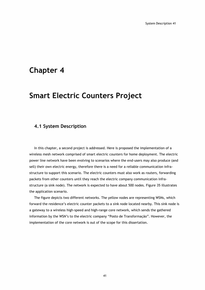
System Description 41
41
Chapter 4
Smart Electric Counters Project
4.1 System Description
In this chapter, a second project is addressed. Here is proposed the implementation of a
wireless mesh network comprised of smart electric counters for home deployment. The electric
power line network have been evolving to scenarios where the end-users may also produce (and
sell) their own electric energy, therefore there is a need for a reliable communication infra-
structure to support this scenario. The electric counters must also work as routers, forwarding
packets from other counters until they reach the electric company communication infra-
structure (a sink node). The network is expected to have about 500 nodes. Figure 35 illustrates
the application scenario.
The figure depicts two different networks. The yellow nodes are representing WSNs, which
forward the residence’s electric counter packets to a sink node located nearby. This sink node is
a gateway to a wireless high-speed and high-range core network, which sends the gathered
information by the WSN’s to the electric company “Posto de Transformação”. However, the
implementation of the core network is out of the scope for this dissertation.
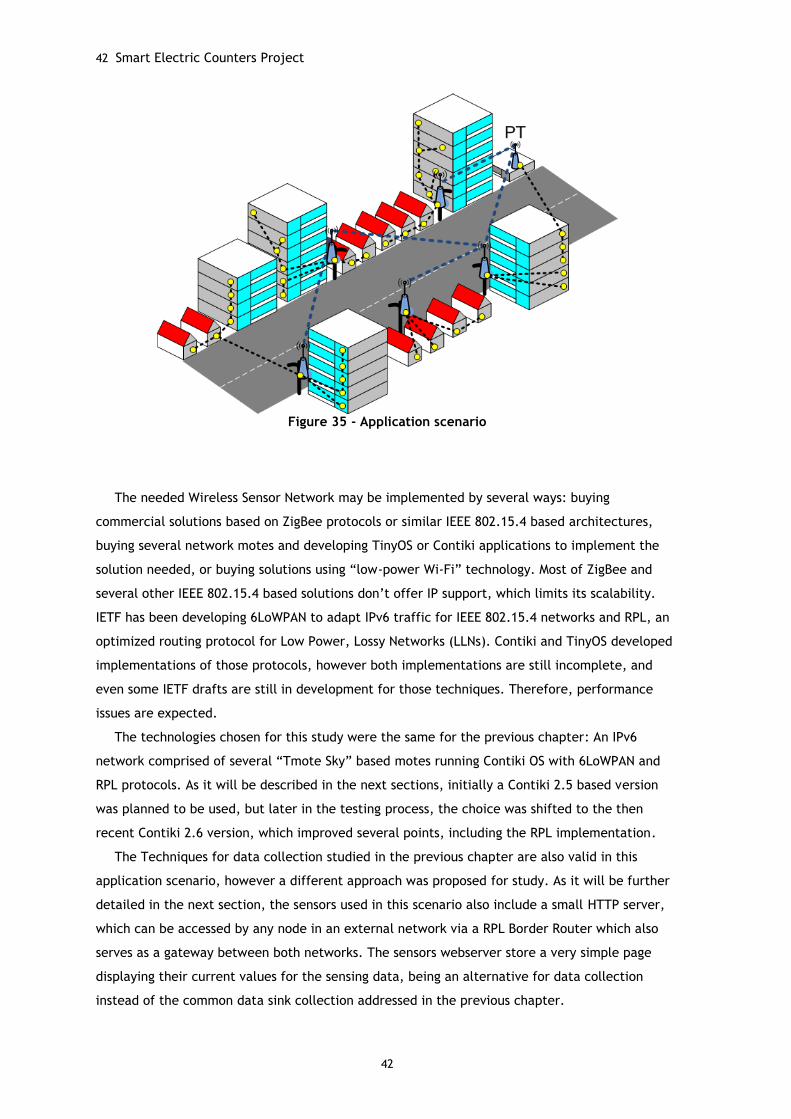
42 Smart Electric Counters Project
42
Figure 35 - Application scenario
The needed Wireless Sensor Network may be implemented by several ways: buying
commercial solutions based on ZigBee protocols or similar IEEE 802.15.4 based architectures,
buying several network motes and developing TinyOS or Contiki applications to implement the
solution needed, or buying solutions using “low-power Wi-Fi” technology. Most of ZigBee and
several other IEEE 802.15.4 based solutions don’t offer IP support, which limits its scalability.
IETF has been developing 6LoWPAN to adapt IPv6 traffic for IEEE 802.15.4 networks and RPL, an
optimized routing protocol for Low Power, Lossy Networks (LLNs). Contiki and TinyOS developed
implementations of those protocols, however both implementations are still incomplete, and
even some IETF drafts are still in development for those techniques. Therefore, performance
issues are expected.
The technologies chosen for this study were the same for the previous chapter: An IPv6
network comprised of several “Tmote Sky” based motes running Contiki OS with 6LoWPAN and
RPL protocols. As it will be described in the next sections, initially a Contiki 2.5 based version
was planned to be used, but later in the testing process, the choice was shifted to the then
recent Contiki 2.6 version, which improved several points, including the RPL implementation.
The Techniques for data collection studied in the previous chapter are also valid in this
application scenario, however a different approach was proposed for study. As it will be further
detailed in the next section, the sensors used in this scenario also include a small HTTP server,
which can be accessed by any node in an external network via a RPL Border Router which also
serves as a gateway between both networks. The sensors webserver store a very simple page
displaying their current values for the sensing data, being an alternative for data collection
instead of the common data sink collection addressed in the previous chapter.
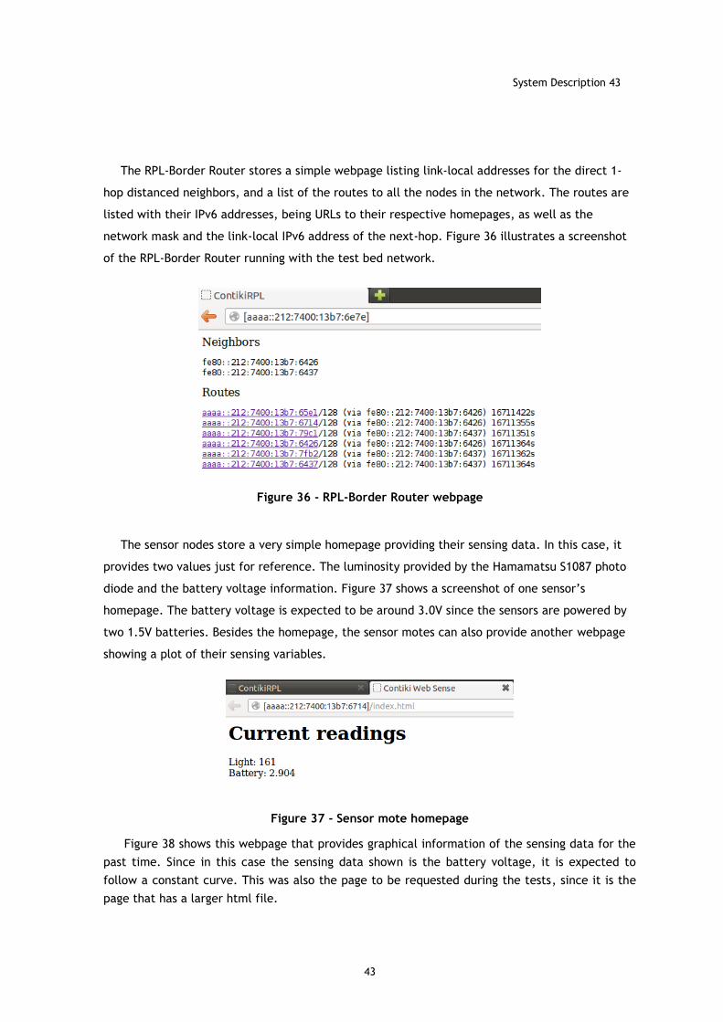
System Description 43
43
The RPL-Border Router stores a simple webpage listing link-local addresses for the direct 1-
hop distanced neighbors, and a list of the routes to all the nodes in the network. The routes are
listed with their IPv6 addresses, being URLs to their respective homepages, as well as the
network mask and the link-local IPv6 address of the next-hop. Figure 36 illustrates a screenshot
of the RPL-Border Router running with the test bed network.
Figure 36 - RPL-Border Router webpage
The sensor nodes store a very simple homepage providing their sensing data. In this case, it
provides two values just for reference. The luminosity provided by the Hamamatsu S1087 photo
diode and the battery voltage information. Figure 37 shows a screenshot of one sensor’s
homepage. The battery voltage is expected to be around 3.0V since the sensors are powered by
two 1.5V batteries. Besides the homepage, the sensor motes can also provide another webpage
showing a plot of their sensing variables.
Figure 37 - Sensor mote homepage
Figure 38 shows this webpage that provides graphical information of the sensing data for the
past time. Since in this case the sensing data shown is the battery voltage, it is expected to
follow a constant curve. This was also the page to be requested during the tests, since it is the
page that has a larger html file.
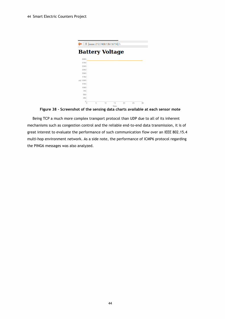
44 Smart Electric Counters Project
44
Figure 38 - Screenshot of the sensing data charts available at each sensor mote
Being TCP a much more complex transport protocol than UDP due to all of its inherent
mechanisms such as congestion control and the reliable end-to-end data transmission, it is of
great interest to evaluate the performance of such communication flow over an IEEE 802.15.4
multi-hop environment network. As a side note, the performance of ICMP6 protocol regarding
the PING6 messages was also analyzed.
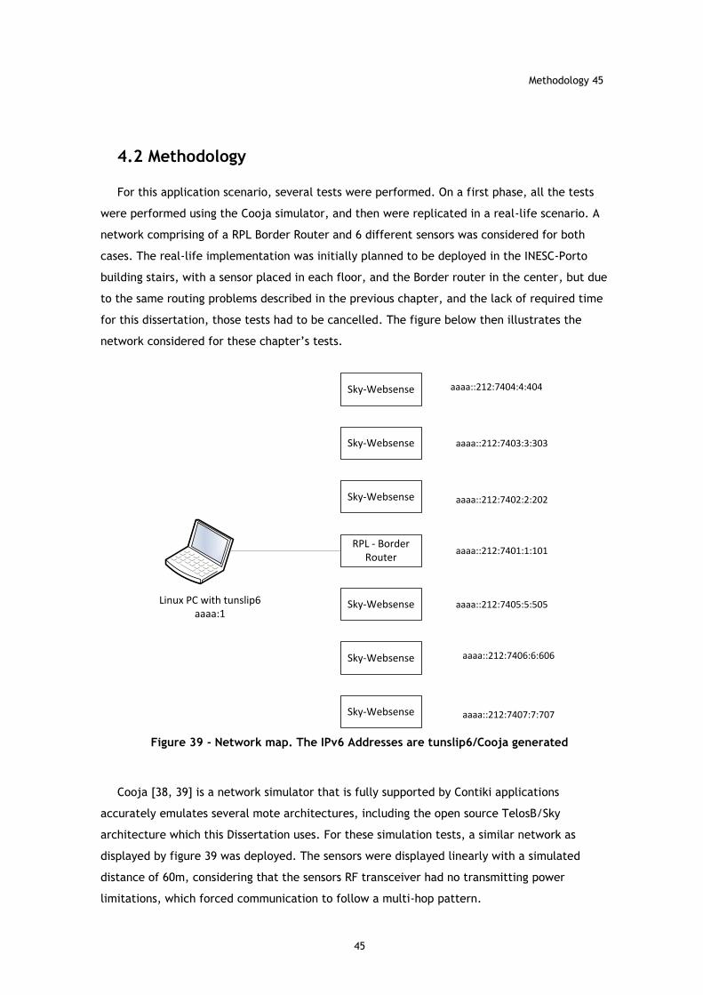
Methodology 45
45
4.2 Methodology
For this application scenario, several tests were performed. On a first phase, all the tests
were performed using the Cooja simulator, and then were replicated in a real-life scenario. A
network comprising of a RPL Border Router and 6 different sensors was considered for both
cases. The real-life implementation was initially planned to be deployed in the INESC-Porto
building stairs, with a sensor placed in each floor, and the Border router in the center, but due
to the same routing problems described in the previous chapter, and the lack of required time
for this dissertation, those tests had to be cancelled. The figure below then illustrates the
network considered for these chapter’s tests.
RPL - Border Router
Sky-Websense
Sky-Websense
Sky-Websense
Sky-Websense
Sky-Websense
Sky-Websense
Linux PC with tunslip6aaaa:1
aaaa::212:7401:1:101
aaaa::212:7405:5:505
aaaa::212:7406:6:606
aaaa::212:7407:7:707
aaaa::212:7402:2:202
aaaa::212:7403:3:303
aaaa::212:7404:4:404
Figure 39 - Network map. The IPv6 Addresses are tunslip6/Cooja generated
Cooja [38, 39] is a network simulator that is fully supported by Contiki applications
accurately emulates several mote architectures, including the open source TelosB/Sky
architecture which this Dissertation uses. For these simulation tests, a similar network as
displayed by figure 39 was deployed. The sensors were displayed linearly with a simulated
distance of 60m, considering that the sensors RF transceiver had no transmitting power
limitations, which forced communication to follow a multi-hop pattern.
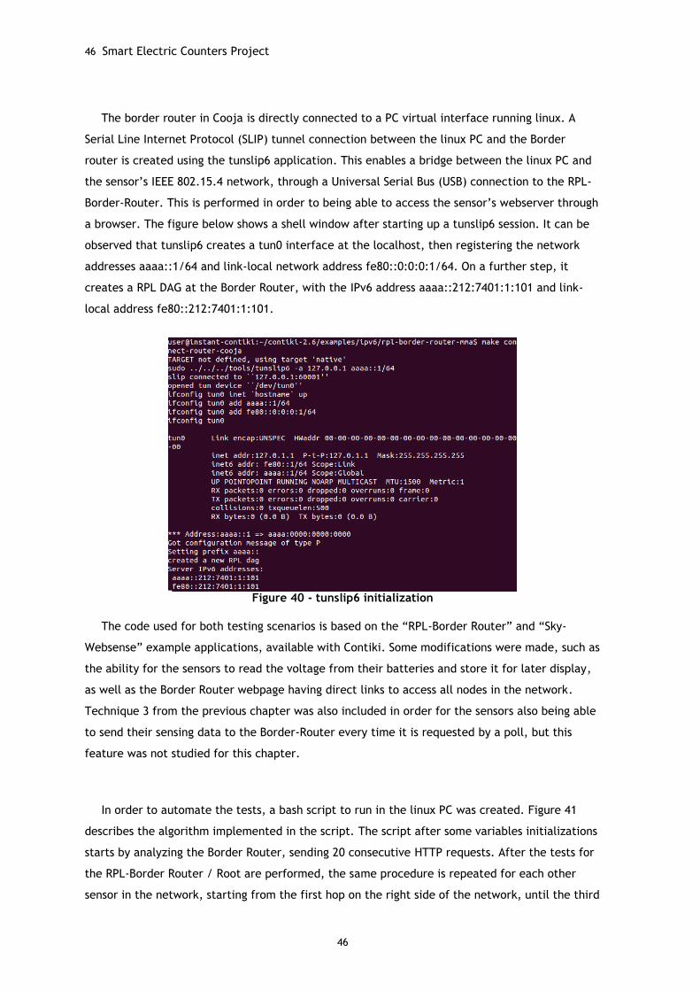
46 Smart Electric Counters Project
46
The border router in Cooja is directly connected to a PC virtual interface running linux. A
Serial Line Internet Protocol (SLIP) tunnel connection between the linux PC and the Border
router is created using the tunslip6 application. This enables a bridge between the linux PC and
the sensor’s IEEE 802.15.4 network, through a Universal Serial Bus (USB) connection to the RPL-
Border-Router. This is performed in order to being able to access the sensor’s webserver through
a browser. The figure below shows a shell window after starting up a tunslip6 session. It can be
observed that tunslip6 creates a tun0 interface at the localhost, then registering the network
addresses aaaa::1/64 and link-local network address fe80::0:0:0:1/64. On a further step, it
creates a RPL DAG at the Border Router, with the IPv6 address aaaa::212:7401:1:101 and link-
local address fe80::212:7401:1:101.
Figure 40 - tunslip6 initialization
The code used for both testing scenarios is based on the “RPL-Border Router” and “Sky-
Websense” example applications, available with Contiki. Some modifications were made, such as
the ability for the sensors to read the voltage from their batteries and store it for later display,
as well as the Border Router webpage having direct links to access all nodes in the network.
Technique 3 from the previous chapter was also included in order for the sensors also being able
to send their sensing data to the Border-Router every time it is requested by a poll, but this
feature was not studied for this chapter.
In order to automate the tests, a bash script to run in the linux PC was created. Figure 41
describes the algorithm implemented in the script. The script after some variables initializations
starts by analyzing the Border Router, sending 20 consecutive HTTP requests. After the tests for
the RPL-Border Router / Root are performed, the same procedure is repeated for each other
sensor in the network, starting from the first hop on the right side of the network, until the third
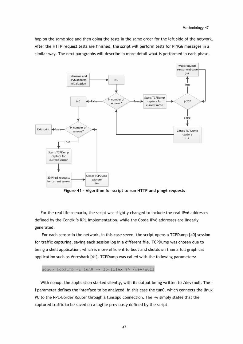
Methodology 47
47
hop on the same side and then doing the tests in the same order for the left side of the network.
After the HTTP request tests are finished, the script will perform tests for PING6 messages in a
similar way. The next paragraphs will describe in more detail what is performed in each phase.
Filename and IPv6 address initialization
i< number of sensors?
Starts TCPDump capture for
current moteTrue j<20?
wget requests sensor webpage
j++
True
Closes TCPDump capture
i++
False
i=0 False
i< number of sensors?
Starts TCPDump capture for
current sensor
True
20 Ping6 requests for current sensor
Closes TCPDump capture
i++
Exit script False
i=0
Figure 41 - Algorithm for script to run HTTP and ping6 requests
For the real life scenario, the script was slightly changed to include the real IPv6 addresses
defined by the Contiki’s RPL implementation, while the Cooja IPv6 addresses are linearly
generated.
For each sensor in the network, in this case seven, the script opens a TCPDump [40] session
for traffic capturing, saving each session log in a different file. TCPDump was chosen due to
being a shell application, which is more efficient to boot and shutdown than a full graphical
application such as Wireshark [41]. TCPDump was called with the following parameters:
nohup tcpdump -i tun0 -w logfilex &> /dev/null
With nohup, the application started silently, with its output being written to /dev/null. The –
i parameter defines the interface to be analyzed, in this case the tun0, which connects the linux
PC to the RPL-Border Router through a tunslip6 connection. The –w simply states that the
captured traffic to be saved on a logfile previously defined by the script.
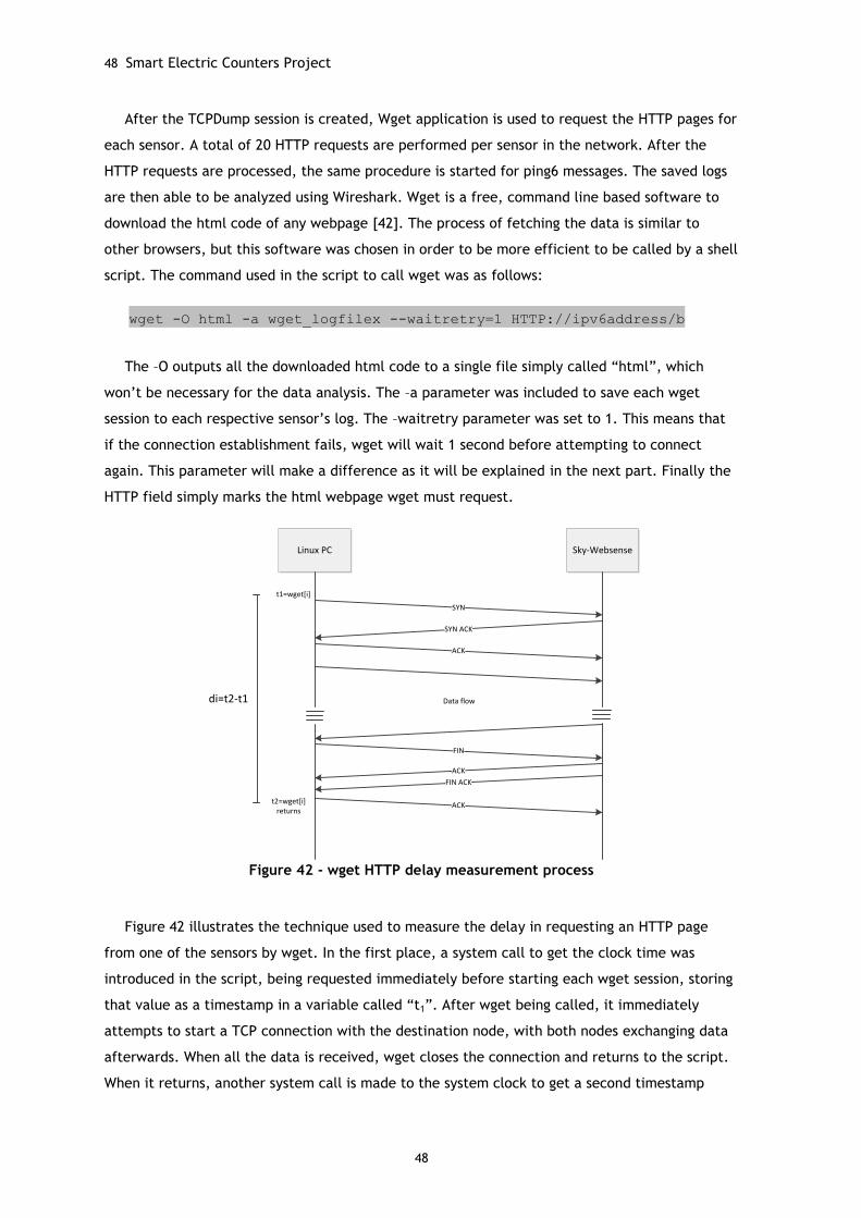
48 Smart Electric Counters Project
48
After the TCPDump session is created, Wget application is used to request the HTTP pages for
each sensor. A total of 20 HTTP requests are performed per sensor in the network. After the
HTTP requests are processed, the same procedure is started for ping6 messages. The saved logs
are then able to be analyzed using Wireshark. Wget is a free, command line based software to
download the html code of any webpage [42]. The process of fetching the data is similar to
other browsers, but this software was chosen in order to be more efficient to be called by a shell
script. The command used in the script to call wget was as follows:
wget -O html -a wget_logfilex --waitretry=1 HTTP://ipv6address/b
The –O outputs all the downloaded html code to a single file simply called “html”, which
won’t be necessary for the data analysis. The –a parameter was included to save each wget
session to each respective sensor’s log. The –waitretry parameter was set to 1. This means that
if the connection establishment fails, wget will wait 1 second before attempting to connect
again. This parameter will make a difference as it will be explained in the next part. Finally the
HTTP field simply marks the html webpage wget must request.
t2=wget[i] returns
Linux PC Sky-Websense
SYN
SYN ACK
ACK
FIN
t1=wget[i]
Data flow
ACK
ACK
FIN ACK
di=t2-t1
Figure 42 - wget HTTP delay measurement process
Figure 42 illustrates the technique used to measure the delay in requesting an HTTP page
from one of the sensors by wget. In the first place, a system call to get the clock time was
introduced in the script, being requested immediately before starting each wget session, storing
that value as a timestamp in a variable called “t1”. After wget being called, it immediately
attempts to start a TCP connection with the destination node, with both nodes exchanging data
afterwards. When all the data is received, wget closes the connection and returns to the script.
When it returns, another system call is made to the system clock to get a second timestamp
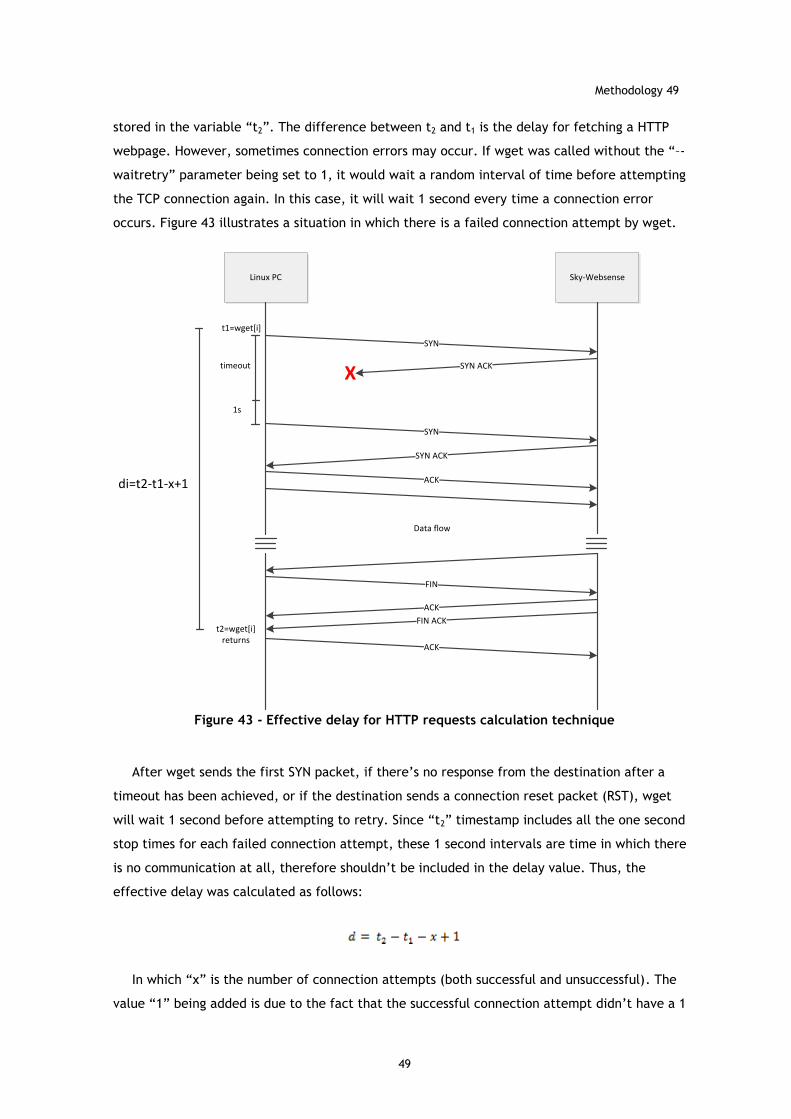
Methodology 49
49
stored in the variable “t2”. The difference between t2 and t1 is the delay for fetching a HTTP
webpage. However, sometimes connection errors may occur. If wget was called without the “–-
waitretry” parameter being set to 1, it would wait a random interval of time before attempting
the TCP connection again. In this case, it will wait 1 second every time a connection error
occurs. Figure 43 illustrates a situation in which there is a failed connection attempt by wget.
t2=wget[i] returns
Linux PC Sky-Websense
SYN
SYN ACK
ACK
FIN
t1=wget[i]
Data flow
ACK
ACK
FIN ACK
di=t2-t1-x+1
X
SYN
SYN ACK
timeout
1s
Figure 43 - Effective delay for HTTP requests calculation technique
After wget sends the first SYN packet, if there’s no response from the destination after a
timeout has been achieved, or if the destination sends a connection reset packet (RST), wget
will wait 1 second before attempting to retry. Since “t2” timestamp includes all the one second
stop times for each failed connection attempt, these 1 second intervals are time in which there
is no communication at all, therefore shouldn’t be included in the delay value. Thus, the
effective delay was calculated as follows:
In which “x” is the number of connection attempts (both successful and unsuccessful). The
value “1” being added is due to the fact that the successful connection attempt didn’t have a 1
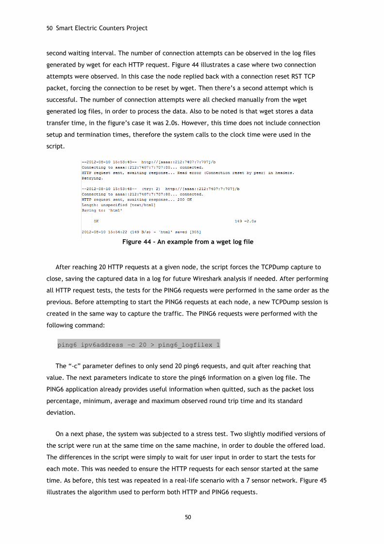
50 Smart Electric Counters Project
50
second waiting interval. The number of connection attempts can be observed in the log files
generated by wget for each HTTP request. Figure 44 illustrates a case where two connection
attempts were observed. In this case the node replied back with a connection reset RST TCP
packet, forcing the connection to be reset by wget. Then there’s a second attempt which is
successful. The number of connection attempts were all checked manually from the wget
generated log files, in order to process the data. Also to be noted is that wget stores a data
transfer time, in the figure’s case it was 2.0s. However, this time does not include connection
setup and termination times, therefore the system calls to the clock time were used in the
script.
Figure 44 - An example from a wget log file
After reaching 20 HTTP requests at a given node, the script forces the TCPDump capture to
close, saving the captured data in a log for future Wireshark analysis if needed. After performing
all HTTP request tests, the tests for the PING6 requests were performed in the same order as the
previous. Before attempting to start the PING6 requests at each node, a new TCPDump session is
created in the same way to capture the traffic. The PING6 requests were performed with the
following command:
ping6 ipv6address –c 20 > ping6_logfilex 1
The “-c” parameter defines to only send 20 ping6 requests, and quit after reaching that
value. The next parameters indicate to store the ping6 information on a given log file. The
PING6 application already provides useful information when quitted, such as the packet loss
percentage, minimum, average and maximum observed round trip time and its standard
deviation.
On a next phase, the system was subjected to a stress test. Two slightly modified versions of
the script were run at the same time on the same machine, in order to double the offered load.
The differences in the script were simply to wait for user input in order to start the tests for
each mote. This was needed to ensure the HTTP requests for each sensor started at the same
time. As before, this test was repeated in a real-life scenario with a 7 sensor network. Figure 45
illustrates the algorithm used to perform both HTTP and PING6 requests.
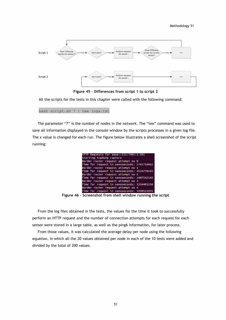
Methodology 51
51
Perform requests for sensor i
Perform requests for sensor i
Start TCPDump session for sensor i?
Start tests?Close TCPDump
session for current sensor?
i++
Start tests? i++
Yes Yes Yes
Yes
Script 1
Script 2
Figure 45 - Differences from script 1 to script 2
All the scripts for the tests in this chapter were called with the following command:
bash script.sh 7 | tee logx.txt
The parameter “7” is the number of nodes in the network. The “tee” command was used to
save all information displayed in the console window by the scripts processes in a given log file.
The x value is changed for each run. The figure below illustrates a shell screenshot of the script
running:
Figure 46 - Screenshot from shell window running the script
From the log files obtained in the tests, the values for the time it took to successfully
perform an HTTP request and the number of connection attempts for each request for each
sensor were stored in a large table, as well as the ping6 information, for later process.
From those values, it was calculated the average delay per node using the following
equation, in which all the 20 values obtained per node in each of the 10 tests were added and
divided by the total of 200 values.
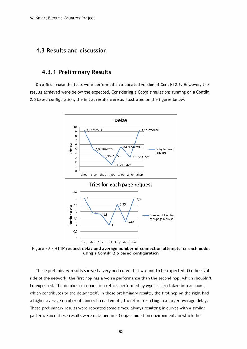
52 Smart Electric Counters Project
52
4.3 Results and discussion
4.3.1 Preliminary Results
On a first phase the tests were performed on a updated version of Contiki 2.5. However, the
results achieved were below the expected. Considering a Cooja simulations running on a Contiki
2.5 based configuration, the initial results were as illustrated on the figures below.
Figure 47 - HTTP request delay and average number of connection attempts for each node,
using a Contiki 2.5 based configuration
These preliminary results showed a very odd curve that was not to be expected. On the right
side of the network, the first hop has a worse performance than the second hop, which shouldn’t
be expected. The number of connection retries performed by wget is also taken into account,
which contributes to the delay itself. In these preliminary results, the first hop on the right had
a higher average number of connection attempts, therefore resulting in a larger average delay.
These preliminary results were repeated some times, always resulting in curves with a similar
pattern. Since these results were obtained in a Cooja simulation environment, in which the
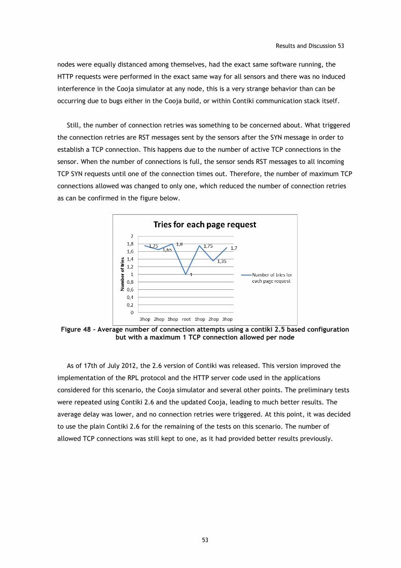
Results and Discussion 53
53
nodes were equally distanced among themselves, had the exact same software running, the
HTTP requests were performed in the exact same way for all sensors and there was no induced
interference in the Cooja simulator at any node, this is a very strange behavior than can be
occurring due to bugs either in the Cooja build, or within Contiki communication stack itself.
Still, the number of connection retries was something to be concerned about. What triggered
the connection retries are RST messages sent by the sensors after the SYN message in order to
establish a TCP connection. This happens due to the number of active TCP connections in the
sensor. When the number of connections is full, the sensor sends RST messages to all incoming
TCP SYN requests until one of the connection times out. Therefore, the number of maximum TCP
connections allowed was changed to only one, which reduced the number of connection retries
as can be confirmed in the figure below.
Figure 48 - Average number of connection attempts using a contiki 2.5 based configuration
but with a maximum 1 TCP connection allowed per node
As of 17th of July 2012, the 2.6 version of Contiki was released. This version improved the
implementation of the RPL protocol and the HTTP server code used in the applications
considered for this scenario, the Cooja simulator and several other points. The preliminary tests
were repeated using Contiki 2.6 and the updated Cooja, leading to much better results. The
average delay was lower, and no connection retries were triggered. At this point, it was decided
to use the plain Contiki 2.6 for the remaining of the tests on this scenario. The number of
allowed TCP connections was still kept to one, as it had provided better results previously.
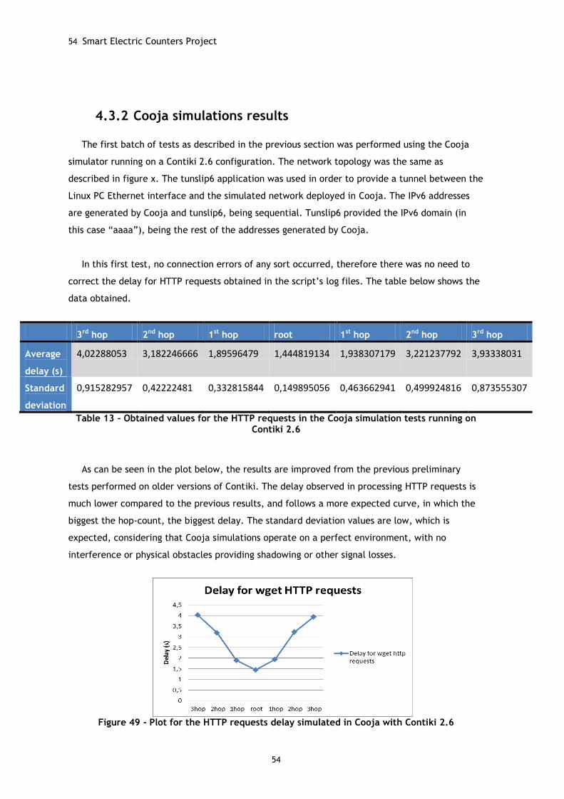
54 Smart Electric Counters Project
54
4.3.2 Cooja simulations results
The first batch of tests as described in the previous section was performed using the Cooja
simulator running on a Contiki 2.6 configuration. The network topology was the same as
described in figure x. The tunslip6 application was used in order to provide a tunnel between the
Linux PC Ethernet interface and the simulated network deployed in Cooja. The IPv6 addresses
are generated by Cooja and tunslip6, being sequential. Tunslip6 provided the IPv6 domain (in
this case “aaaa”), being the rest of the addresses generated by Cooja.
In this first test, no connection errors of any sort occurred, therefore there was no need to
correct the delay for HTTP requests obtained in the script’s log files. The table below shows the
data obtained.
3rd hop 2nd hop 1st hop root 1st hop 2nd hop 3rd hop
Average
delay (s)
4,02288053 3,182246666 1,89596479 1,444819134 1,938307179 3,221237792 3,93338031
Standard
deviation
0,915282957 0,42222481 0,332815844 0,149895056 0,463662941 0,499924816 0,873555307
Table 13 - Obtained values for the HTTP requests in the Cooja simulation tests running on Contiki 2.6
As can be seen in the plot below, the results are improved from the previous preliminary
tests performed on older versions of Contiki. The delay observed in processing HTTP requests is
much lower compared to the previous results, and follows a more expected curve, in which the
biggest the hop-count, the biggest delay. The standard deviation values are low, which is
expected, considering that Cooja simulations operate on a perfect environment, with no
interference or physical obstacles providing shadowing or other signal losses.
Figure 49 - Plot for the HTTP requests delay simulated in Cooja with Contiki 2.6
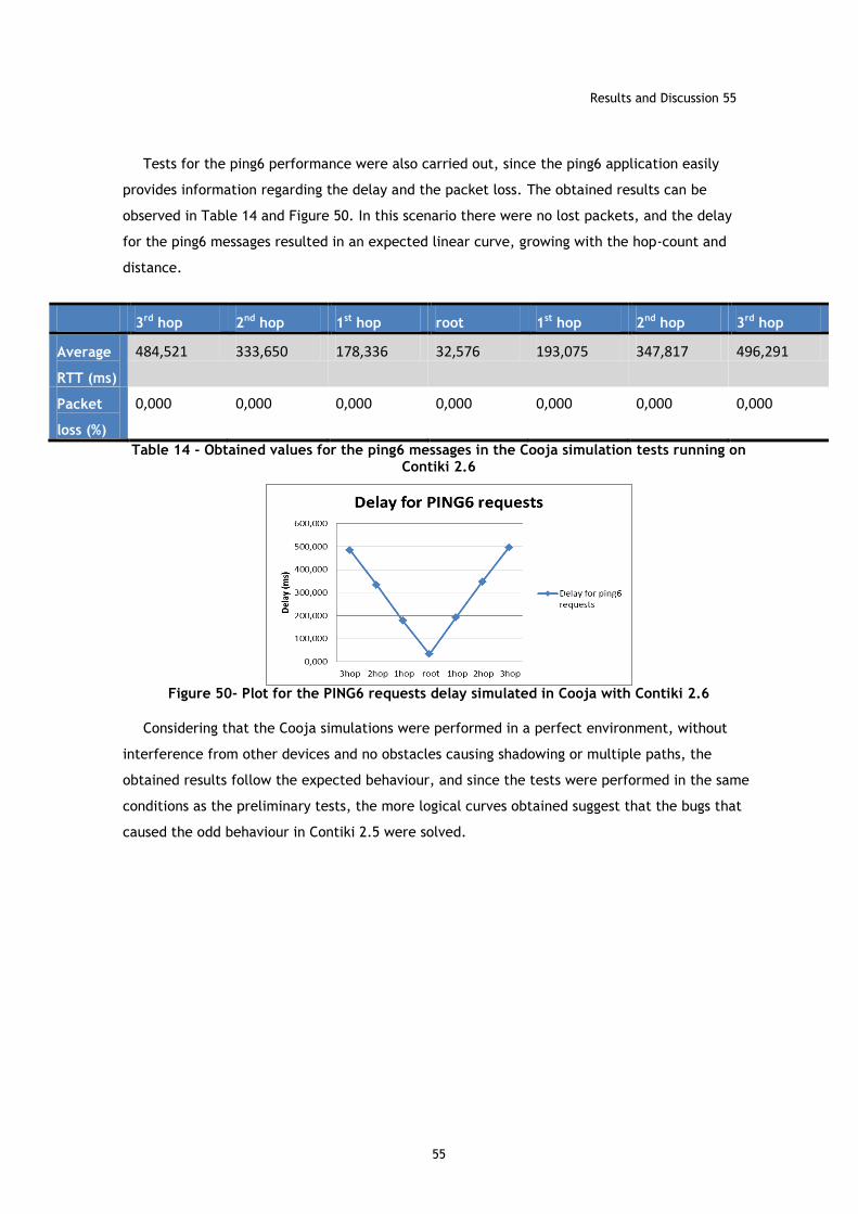
Results and Discussion 55
55
Tests for the ping6 performance were also carried out, since the ping6 application easily
provides information regarding the delay and the packet loss. The obtained results can be
observed in Table 14 and Figure 50. In this scenario there were no lost packets, and the delay
for the ping6 messages resulted in an expected linear curve, growing with the hop-count and
distance.
3rd hop 2nd hop 1st hop root 1st hop 2nd hop 3rd hop
Average
RTT (ms)
484,521 333,650 178,336 32,576 193,075 347,817 496,291
Packet
loss (%)
0,000 0,000 0,000 0,000 0,000 0,000 0,000
Table 14 - Obtained values for the ping6 messages in the Cooja simulation tests running on Contiki 2.6
Figure 50- Plot for the PING6 requests delay simulated in Cooja with Contiki 2.6
Considering that the Cooja simulations were performed in a perfect environment, without
interference from other devices and no obstacles causing shadowing or multiple paths, the
obtained results follow the expected behaviour, and since the tests were performed in the same
conditions as the preliminary tests, the more logical curves obtained suggest that the bugs that
caused the odd behaviour in Contiki 2.5 were solved.
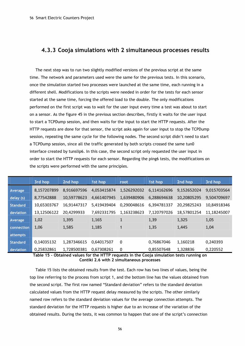
56 Smart Electric Counters Project
56
4.3.3 Cooja simulations with 2 simultaneous processes results
The next step was to run two slightly modified versions of the previous script at the same
time. The network and parameters used were the same for the previous tests. In this scenario,
once the simulation started two processes were launched at the same time, each running in a
different shell. Modifications to the scripts were needed in order for the tests for each sensor
started at the same time, forcing the offered load to the double. The only modifications
performed on the first script was to wait for the user input every time a test was about to start
on a sensor. As the figure 45 in the previous section describes, firstly it waits for the user input
to start a TCPDump session, and then waits for the input to start the HTTP requests. After the
HTTP requests are done for that sensor, the script asks again for user input to stop the TCPDump
session, repeating the same cycle for the following nodes. The second script didn’t need to start
a TCPDump session, since all the traffic generated by both scripts crossed the same tun0
interface created by tunslip6. In this case, the second script only requested the user input in
order to start the HTTP requests for each sensor. Regarding the ping6 tests, the modifications on
the scripts were performed with the same principles.
3rd hop 2nd hop 1st hop root 1st hop 2nd hop 3rd hop
Average
delay (s)
8,157207899
8,77542888
8,916697596
10,59778623
4,053415874
4,661407945
1,526292032
1,639480906
6,114162696
6,288694638
9,152652024
10,20805295
9,015703564
9,504709697
Standard
deviation
10,65303767
13,12506122
16,91447317
20,4299933
5,419439404
7,692331795
0,290048616
1,163238623
6,394781337
7,120797026
20,29825243
18,57801254
10,84918346
11,18245007
Average
connection
attempts
1,02
1,06
1,395
1,585
1,165
1,185
1
1
1,39
1,35
1,325
1,445
1,05
1,04
Standard
deviation
0,14035132
0,25832861
1,287346615
1,728500381
0,64017507
0,67308261
0
0
0,76867046
0,85507648
1,160218
1,328836
0,240393
0,220552
Table 15 - Obtained values for the HTTP requests in the Cooja simulation tests running on Contiki 2.6 with 2 simultaneous processes
Table 15 lists the obtained results from the test. Each row has two lines of values, being the
top line referring to the process from script 1, and the bottom line has the values obtained from
the second script. The first row named “Standard deviation” refers to the standard deviation
calculated values from the HTTP request delay measured by the scripts. The other similarly
named row refers to the standard deviation values for the average connection attempts. The
standard deviation for the HTTP requests is higher due to an increase of the variation of the
obtained results. During the tests, it was common to happen that one of the script’s connection
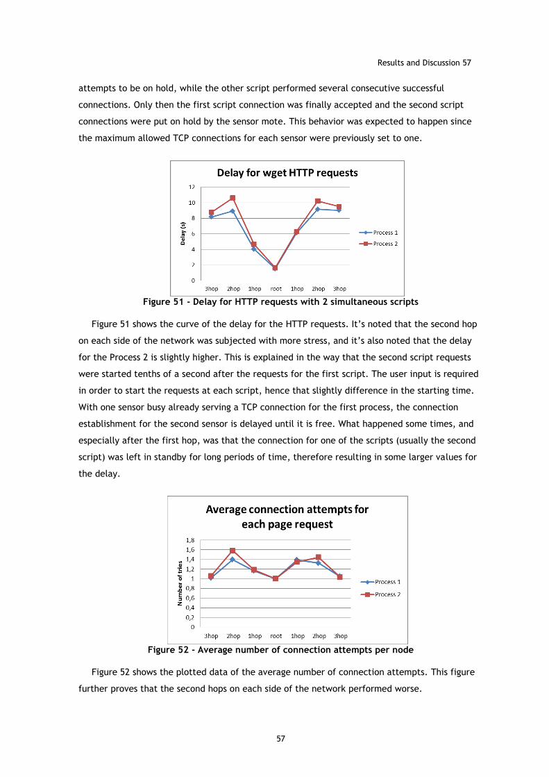
Results and Discussion 57
57
attempts to be on hold, while the other script performed several consecutive successful
connections. Only then the first script connection was finally accepted and the second script
connections were put on hold by the sensor mote. This behavior was expected to happen since
the maximum allowed TCP connections for each sensor were previously set to one.
Figure 51 - Delay for HTTP requests with 2 simultaneous scripts
Figure 51 shows the curve of the delay for the HTTP requests. It’s noted that the second hop
on each side of the network was subjected with more stress, and it’s also noted that the delay
for the Process 2 is slightly higher. This is explained in the way that the second script requests
were started tenths of a second after the requests for the first script. The user input is required
in order to start the requests at each script, hence that slightly difference in the starting time.
With one sensor busy already serving a TCP connection for the first process, the connection
establishment for the second sensor is delayed until it is free. What happened some times, and
especially after the first hop, was that the connection for one of the scripts (usually the second
script) was left in standby for long periods of time, therefore resulting in some larger values for
the delay.
Figure 52 - Average number of connection attempts per node
Figure 52 shows the plotted data of the average number of connection attempts. This figure
further proves that the second hops on each side of the network performed worse.
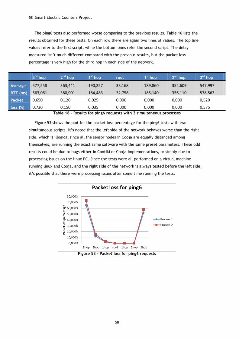
58 Smart Electric Counters Project
58
The ping6 tests also performed worse comparing to the previous results. Table 16 lists the
results obtained for these tests. On each row there are again two lines of values. The top line
values refer to the first script, while the bottom ones refer the second script. The delay
measured isn’t much different compared with the previous results, but the packet loss
percentage is very high for the third hop in each side of the network.
3rd hop 2nd hop 1st hop root 1st hop 2nd hop 3rd hop
Average
RTT (ms)
577,558
563,061
363,441
380,901
190,257
184,483
33,168
32,758
189,860
185,140
352,609
356,110
547,997
578,563
Packet
loss (%)
0,650
0,730
0,120
0,150
0,025
0,035
0,000
0,000
0,000
0,000
0,000
0,000
0,520
0,575
Table 16 - Results for ping6 requests with 2 simultaneous processes
Figure 53 shows the plot for the packet loss percentage for the ping6 tests with two
simultaneous scripts. It’s noted that the left side of the network behaves worse than the right
side, which is illogical since all the sensor nodes in Cooja are equally distanced among
themselves, are running the exact same software with the same preset parameters. These odd
results could be due to bugs either in Contiki or Cooja implementations, or simply due to
processing issues on the linux PC. Since the tests were all performed on a virtual machine
running linux and Cooja, and the right side of the network is always tested before the left side,
it’s possible that there were processing issues after some time running the tests.
Figure 53 - Packet loss for ping6 requests
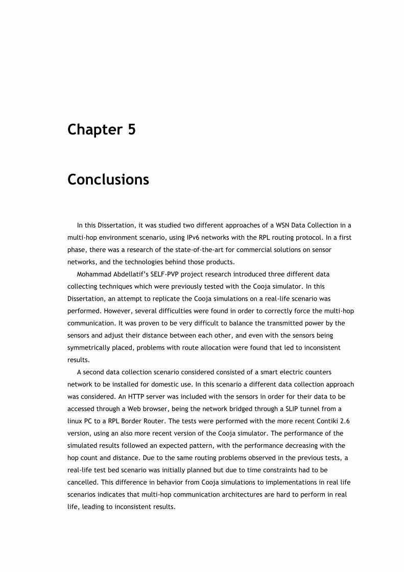
Chapter 5
Conclusions
In this Dissertation, it was studied two different approaches of a WSN Data Collection in a
multi-hop environment scenario, using IPv6 networks with the RPL routing protocol. In a first
phase, there was a research of the state-of-the-art for commercial solutions on sensor
networks, and the technologies behind those products.
Mohammad Abdellatif’s SELF-PVP project research introduced three different data
collecting techniques which were previously tested with the Cooja simulator. In this
Dissertation, an attempt to replicate the Cooja simulations on a real-life scenario was
performed. However, several difficulties were found in order to correctly force the multi-hop
communication. It was proven to be very difficult to balance the transmitted power by the
sensors and adjust their distance between each other, and even with the sensors being
symmetrically placed, problems with route allocation were found that led to inconsistent
results.
A second data collection scenario considered consisted of a smart electric counters
network to be installed for domestic use. In this scenario a different data collection approach
was considered. An HTTP server was included with the sensors in order for their data to be
accessed through a Web browser, being the network bridged through a SLIP tunnel from a
linux PC to a RPL Border Router. The tests were performed with the more recent Contiki 2.6
version, using an also more recent version of the Cooja simulator. The performance of the
simulated results followed an expected pattern, with the performance decreasing with the
hop count and distance. Due to the same routing problems observed in the previous tests, a
real-life test bed scenario was initially planned but due to time constraints had to be
cancelled. This difference in behavior from Cooja simulations to implementations in real life
scenarios indicates that multi-hop communication architectures are hard to perform in real
life, leading to inconsistent results.
60 Conclusions
60
But since technologies such as 6LoWPAN and RPL are still very recent, and their ports for
Contiki Operating System are yet not complete, performance issues were still expected to be
found.
Even so, with erratic results, and without necessarily resorting to multi-hop
communication, the nodes can communicate with each other, even if there’s a low
performance. Also to be taken in consideration is the offered load in the network. In most of
WSNs it is not required that the sensors transmit their information at rates higher than one
packet per second. Most of the time the sensors are in sleep mode, only sending their sensing
data once in a while. Since the sensors are equipped with very low processing power and
available RAM, it’s expected the network to perform worse when in more stressful
environments.
As future work, more tests should be done using different transmitting powers and
placement of the sensors in order to find an optimal sensor distribution to correctly perform
multi-hop communication. There should also be some debugging at the RPL and MAC level in
order to find and fix the routing issues.
Testing the performance of the network without resorting to a forced multi-hop
communication should also be considered. A more realistic test bed such as an inner staircase
of a building for the smart electric counters should be considered, placing the sensors at one
floor each, without limitations in the transmitted power or in the number of neighbors per
each node.
References
[1] Contiki. (2008). 6LoWPAN implementation. Available: http://www.sics.se/~adam/contiki/docs-uipv6/a01109.html
[2] Y. Chen, H. Kun-Mean, Z. Haiying, S. Hong-ling, L. Xing, D. Xunxing, D. Hao, L. Jian-Jin, and C. de Vaulx, "6LoWPAN Stacks: A Survey," in Wireless Communications, Networking and Mobile Computing (WiCOM), 2011 7th International Conference on, 2011, pp. 1-4.
[3] R. Silva, JS Silva, and Fernando Boavida, "Evaluating 6lowPAN implementations in WSNs," in Proceedings of 9th Conferncia sobre Redes de Computadores, Oeiras Portugal, 2009, pp. 1-5.
[4] J. Ko, J. Eriksson, N. Tsiftes, S. Dawson-Haggerty, A. Terzis, A. Dunkels, and D. Culler. (2011, ContikiRPL and TinyRPL: Happy Together. Available: http://www.sics.se/~adam/ko11contikirpl.pdf
[5] L. Adams. (2007, Capitalizing on 802.11 For Sensor Networks. Available: http://www.gainspan.com/docs2/GS_80211_networks-WP.pdf
[6] G. Corporation. (2011, GS1011 Ultra Low-Power Wireless System on Chip (SoC) Available: http://www.gainspan.com/docs2/GS1011-PB.pdf
[7] D. M. Dobkin and B. Aboussouan. (2009, Low Power Wi-Fi™ (IEEE 802.11) For IP Smart Objects. Available: http://www.gainspan.com/docs2/Low_Power_Wi-Fi_for_Smart_IP_Objects_WP_cmp.pdf
[8] G. Corporation. 11b is better. Available: http://www.gainspan.com/docs2/11b_is_Better_v1_0.pdf
[9] R. Signals. (2008, SenSiFi Product Brief. Available: http://www.redpinesignals.com/pdfs/RS9110-N-11-31.pdf
[10] R. Signals. (2010). Why 11n? Available: http://www.redpinesignals.com/Solutions/Wi-Fi_Design_Center/why11n.html
[11] B. D. Ltd. ZMM-01 ZigBee Smart Energy Module. Available: http://www.bytesnap.co.uk/assets/Uploads/Documents/ZMM01/Module-Brief-v2-0-Sept2011-FINAL.pdf
[12] "IEEE Standard for Information Technology- Telecommunications and Information Exchange Between Systems- Local and Metropolitan Area Networks- Specific Requirements Part 15.4: Wireless Medium Access Control (MAC) and Physical Layer (PHY) Specifications for Low-Rate Wireless Personal Area Networks (WPANs)," IEEE Std 802.15.4-2006 (Revision of IEEE Std 802.15.4-2003), pp. 0_1-305, 2006.
[13] N. Salman, I. Rasool, and A. H. Kemp, "Overview of the IEEE 802.15.4 standards family for Low Rate Wireless Personal Area Networks," in Wireless Communication Systems (ISWCS), 2010 7th International Symposium on, 2010, pp. 701-705.
[14] "IEEE Standard for Information Technology - Telecommunications and Information Exchange Between Systems - Local and Metropolitan Area Networks - Specific Requirement Part 15.4: Wireless Medium Access Control (MAC) and Physical Layer (PHY) Specifications for Low-Rate Wireless Personal Area Networks (WPANs)," IEEE Std 802.15.4a-2007 (Amendment to IEEE Std 802.15.4-2006), pp. 1-203, 2007.
[15] "IEEE Standard for Information technology-Telecommunications and information exchange between systems-Local and metropolitan area networks-Specific
62
requirements Part 15.4: Wireless Medium Access Control (MAC) and Physical Layer (PHY) Specifications for Low-Rate Wireless Personal Area Networks (WPANs) Amendment 3: Alternative Physical Layer Extension to support the Japanese 950 MHz bands," IEEE Std 802.15.4d-2009 (Amendment to IEEE Std 802.15.4-2006), pp. c1-27, 2009.
[16] "IEEE Standard for Information technology-Telecommunications and information exchange between systems-Local and metropolitan area networks-Specific requirements Part 15.4: Wireless Medium Access Control (MAC) and Physical Layer (PHY) Specifications for Low-Rate Wireless Personal Area Networks (WPANs) Amendment 2: Alternative Physical Layer Extension to support one or more of the Chinese 314-316 MHz, 430-434 MHz, and 779-787 MHz bands," IEEE Std 802.15.4c-2009 (Amendment to IEEE Std 802.15.4-2006), pp. c1-21, 2009.
[17] M. Ricardo, "Wireless Local Area Networks Wireless Personal Area Networks," in Acetatos de Comunicações Móveis, ed. FEUP, 2009/10. [18] G. Montenegro, N. Kushalnagar, J. Hui, and D. Culler, "Transmission of IPv6 Packets
over IEEE 802.15.4 Networks," ed. IETF RFC4994, 2007. [19] Z. Shelby and C. Bormann, 6LoWPAN: The Wireless Embedded Internet. Wiley
Publishing, 2010. [20] J. Hui and D. Culler, "6LoWPAN: Incorporating IEEE 802.15.4 into the IP architecture,"
ed. Internet Protocol for Smart Objects (IPSO) Alliance, White paper # 3, 2009. [21] Z. Shelby, S. Chakrabarti, and E. Nordmark, "Neighbor Discovery Optimization for Low
Power and Lossy Networks," ed. draft-ietf-6lowpan-nd-18: work in progress, IETF, 2011.
[22] C. Bormann. (2011, Getting Started with IPv6 in Low-P ower Wireless “Personal Area” Networks (6LoWPAN). Available: http://6lowpan.net/wp-content/uploads/2011/03/6lowpan-tutorial-ietf80-7-sanitized.pdf
[23] A. H. Chowdhury, M. Ikram, H.-S. Cha, H. Redwan, S. M. S. Shams, K.-H. Kim, and S.-W. Yoo, "Route-over vs mesh-under routing in 6LoWPAN," presented at the Proceedings of the 2009 International Conference on Wireless Communications and Mobile Computing: Connecting the World Wirelessly, Leipzig, Germany, 2009.
[24] T. Winter, P. Thubert, A. Brandt, J. Hui, R. Kelsey, P. Levis, K. Pister, R. Struik, J. Vasseur, and R. Alexander, "RPL: IPv6 Routing Protocol for Low power and Lossy Networks," ed. RFC6550: IETF.
[25] J. Vasseur, N. Agarwal, J. Hui, Z. Shelby, P. Bertrand, and C. Chauvenet, "RPL: The IP routing protocol designed for low power and lossy networks," Internet Protocol for Smart Objects (IPSO) Alliance, 2011.
[26] J. Hui, "RPL: IPv6 Routing Protocol for Low Power and Lossy Networks, ROLL WG Meeting, 76th IETF Meeting, Hiroshima, Japan," ed, 2009.
[27] M. Goyal, E. Baccelli, M. Philipp, A. Brandt, and J. Martocci, "Reactive Discovery of Point-to-Point Routes in Low Power and Lossy Networks," draft-ietf-roll-p2p-rpl-07, work in progress, IETF, 2012.
[28] I. S. Association. (Fevereiro 7). IEEE 802.11™: WIRELESS LOCAL AREA NETWORKS (LANs). Available: http://standards.ieee.org/about/get/802/802.11.html
[29] J. Ruela, "Wireless LANs - IEEE 802.11 e 802.11e," in Acetatos de Redes de Banda Larga, ed. FEUP, 2009/10.
[30] J. M. Tjensvold. (2007, IEEE Standard for Comparison of the IEEE 802.11, 802.15.1, 802.15.4 and 802.15.6 wireless standards. Available: http://janmagnet.files.wordpress.com/2008/07/comparison-ieee-802-standards.pdf
[31] E. Perahia, "IEEE 802.11n Development: History, Process, and Technology," Communications Magazine, IEEE, vol. 46, pp. 48-55, 2008.
[32] W. C. Craig, "ZigBee: "Wireless Control that Simply Works"," 2004. [33] S. Ashton, "ZigBee Technology Overview," 2009. [34] I. Mardsen, "ZigBee Alliance - Network Layer Overview," Embedded Systems Show,
Birmingham, 2006. [35] Crossbow. TelosB Mote Platform. Available:
http://www.willow.co.uk/TelosB_Datasheet.pdf [36] Advanticsys, "MTM-CM5000-MSP Features." [37] J. O. Mohammad Abdellatif, Manuel Ricardo, Peter Steenkiste, "Impact of Data
Collecting Techniques on the Performance of a Wireless Sensor Network," presented
References 63
63
at the Proceedings of the ISWCS 2012, the Ninth International Symposium on Wireless Communication Systems, Paris, France, August 28-31, 2012.
[38] COOJA. Available: http://wiki.contiki-os.org/doku.php?id=an_introduction_to_cooja [39] F. Österlind, "A Sensor Network Simulator for the Contiki OS," SICS2006. [40] TCPDump. TCPDump software. Available: http://www.tcpdump.org/ [41] Wireshark. Wireshark software. Available: http://www.wireshark.org/ [42] Wget. Wget software. Available: http://www.gnu.org/software/wget/