Wireless Network Capacity

8/3/2019 Wireless Network Capacity

http://slidepdf.com/reader/full/wireless-network-capacity 1/142

A (Cynic‟s) Recent History of Wireless Network Capacity

Research

Stavros Toumpis(Informatics Dept., ΩΠΑ!)

TUC, Summer 2010

1



Organization

1. Introduction2. A few basic questions

3. Asymptotic Capacity of Wireless

Networks with Immobile Nodes

4. Asymptotic Capacity of Wireless

Networks with Mobile Nodes

5. Capacity of Massive Wireless Networks

2

P R OB A

B I L I S T I C

T O

OL S

OP

T I MI Z A T I ON

T O OL S



1. Introduction

3



Cellular Wireless Networks

• Mobile terminals communicate with othersexclusively through base stations.

• Mobile terminals have very little responsibility.

• A wireless access network.

PSTN,

Internet,

etc.

Α Β



Truly Wireless Networks

• Mobile Terminals communicate through their

neighbors.• Mobile Terminals have many responsibilities.

– For example, they must forward other terminals‟ data.

• Much more challenging.

PSTN,

Internet,

etc.

Α

Β



Prehistory

• Research started in the 70‟s – ARPA Project

– Some military communications systems came outof it (ΕΡΜΗ!)

• Interest cooled off in the 80‟s

• Renewed interest in the 90‟s – Wireless communications very popular

– Technology became more powerful and couldsupport algorithms.

• Currently, interest is still going strong.

6



Preprehistory : NavalCommunications at

the Turn of the(Previous) Century

• Problem: Stop the German High Seas

Fleet going in/out of Denmark Strait• Setting:

– You are in 1914, most of your ships have no wireless. Must

depend on visual communication.

– Fog, i.e., fading

• Solution: A Hierarchical, Mobile, Visual Sensor

Network.

• Many other examples in history, even in antiquity 7

http://en.wikipedia.org/wiki/History_of_communication

http://en.wikipedia.org/wiki/History_of_communication



Many names for the same thing

1. Packet Radio Networks (70‟s)2. Multihop Wireless Networks (80‟s)3. Wireless ad hoc networks (90‟s)

– Mostly EE people4. Mobile Ad Hoc Networks - MANETs (90‟s)

– Mostly CS people

5. Wireless Networks (future?)

Question: What do you think is the reason for this constant change of names?

8



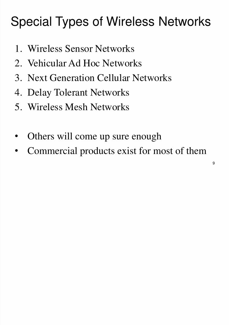
Special Types of Wireless Networks

1. Wireless Sensor Networks

2. Vehicular Ad Hoc Networks

3. Next Generation Cellular Networks4. Delay Tolerant Networks

5. Wireless Mesh Networks

• Others will come up sure enough

• Commercial products exist for most of them9



1. Wireless Sensor Networks

SINK

SINK

Task Manager

Internet,Satellite,

UAV



• Applications:

– Sensing forest fires – Monitoring earthquakes

– Military applications

– Agricultural Applications• Challenges

– Integrate data collection / compression with

communications

– Low energy

– High lifetime requirement

11

http://www.tovima.gr/default.asp?pid=2&artid=337579&ct=1&dt=15/06/2010

http://www.tovima.gr/default.asp?pid=2&artid=337579&ct=1&dt=15/06/2010



2. Wireless Mesh Networks

INTERNET

Question: Why do you think AMWN is so large?

http://www.awmn.net/

http://www.awmn.net/



3. Next Generation Wireless Access

(Hybrid) Networks

Under current 3G technology, mobilephones only communicate with thebase stations

In next generation wireless accessnetworks, mobile terminals willexchange information directly witheach other, saving energy andbandwidth.

With 3G technology, user A looses

connectivity

Α

Β

In next generation networks, userB will forward user A‟s data

http://www.wireless-world-research.org/index.php?id=141







4. Vehicular Ad Hoc Networks

(VANETs)



• Applications

– Security (for example, car notifies when there is an

accident 300 meters ahead)

– Infotainment

• Challenges

– Topology changes fast

– Security, QoS

• Obvious interest from auto companies

15

http://www.worldcarfans.com/10510278356/general-motors-develops-vehicle-to-vehicle-communication

http://www.worldcarfans.com/10510278356/general-motors-develops-vehicle-to-vehicle-communication



5. Delay Tolerant Networks

• Basic Idea: Delays in the communication areso large, topology changes

• Some times, delays are unavoidable

– Partitioned Networks

• Some times, delays are acceptable

– Data is not time critical

• Applications – Space telecommunication

– Wildlife tracking, for zebras, whales, etc.

16

http://papers/fall03.pdf

http://papers/space.pdf

http://papers/zebranet.pdf

http://papers/whales.pdf







Peculiarities of the wireless channel

1. Communication links are coupled

– i.e., wireless medium is inherently broadcast

2. Bandwidth is limited

– 106

times less bandwidth than optical networks3. Communication is localized, because signals decay

with distance

– The graphs that describes who can talk to whom directly is

embedded in a 2D space.

Question: Which one do you think is the mostimportant from a networking perspective?

17



Two Main Research Areas

• Protocols research: Trying to achieve the

capacity

– Media Access, Routing, Transport, etc.

– Also cross layer: Routing/MAC protocols, etc.

• Capacity research: trying to find the capacity

in the first place

18



Caveat: Capacity means different

things to different people

• Information Theoretic Capacity

– “What is the maximum rate of communication under allmodulation schemes in the AWGN channel?”

• Media Access Capacity – “What is the maximum probability of success in Slotted

Aloha?”

• Cellular Capacity („When not to spread spectrum…‟)

• Erlang Capacity

– “How many restrooms do I need a cinema with 500 seats,so that blockage probability is less than 1%”?

• Network Capacity 19



Network Capacity (roughly)

• Consider a complete network model:

– Node placements (regular, arbitrary)

– Channel/Transceiver model (see next slides)

– Assume perfect coordination:

– Perfect medium access (we never have collisions) – Optimal routing (no routing overhead)

– Perfect power control (no unnecessary interference anywhere)

• How to think about: GOD tells everyone when to transmit,

to whom, what data, with what power, rate, etc.

• Network Capacity is the traffic carrying capability of the

network under this condition.

20



• Network Capacity Research is necessarily cross-layer.

• We need to simplify! Otherwise the problem becomes

impossible to solve.

• Next, we see two common simplifications1 of the

PHY layer (Information Theorists, brace yourselves.)1. “Protocol Model”

2. “Physical Model”

– Also known as SINR model and Interference Model

• Others exist. They all exhibit tradeoff

between accuracy and simplicity

21

1 P. Gupta and P. R. Kumar, „The Capacity of Wireless Networks,‟IEEE Trans. On Information Theory, Vol. 46, No. 2, Mar. 2000, pp 388-404.

Simplified PHY

http://papers/gupta_kumar.pdf











1. Protocol Model

• A transmission from node X i to node X j is

successful iff

– | X i - X j |<r

– For all other simultaneously transmitting nodes X k

we have | X k - X j |>(1+Δ)r (First Option)

– For all other simultaneously transmitting nodes X k

we have | X k - X j |>(1+Δ) | X i - X j | (Second Option)• All transmissions are with rate W

22



Critique

• According to the model, the transmission onthe left is a success, and that on the right leads

to a collision.

• In reality, the inverse is more probable. 23



2. Physical Model

• When node X i transmits with power Pi, node X jreceives a signal with power Pr,j=GijPi.

– Commonly, Gij=K(d ij)-a , a>2

• Reception in node X j is successful provided that

R j ≤ f R(γ j ) ≡Wlog 2(1+γ j / Γ )

where

γ j = GijPi /(η+ Σ k ϵ T , k ≠i Gkj Pk )

and T is the set of transmitting nodes.

• Obviously more realistic than protocol model. Effects

of interference are now additive.

24



2. A few basic questions

25



Basic Question 1

• Assume a source, a sink, and many nodes inbetween that can act as relays.

• Basic Question 1: Is it better to transmit withone long hop, or with many small ones?

• An obvious tradeoff exists: – With one long hops, you use the channel once, but

need to transmit with high power, so you interferemore.

– With many short hops, you transmit many times, butwith less power.

– Is there a “sweet spot”?

26



Answer

• Many small hops are better,because they occupy less area.

• Unfortunately, this complicates

both the design protocols and the

capacity calculationstremendously.

• Explanation carries through

under most reasonable models.• Two basic resources: Bandwidth

and Area!!

27



Basic Question 2

• Basic Question 2: So, given we use shorthops (see Basic Question 1) how many hopson the average is the distance between twonodes in a network of n nodes?

• If all nodes were on a square grid, we wouldneed on the order of n1/2 hops

• But this is too restricting.

• What happens when nodes are placedrandomly?

28



Quick Lemma

• n nodes

• n/(k 1log n) cells C

1 ,C

2 ,…

• m j nodes in cell C j

• On the average we have

k 1log n nodes per cell• In fact, something stronger holds:

P{k 1log n /2 ≤ m j ≤2k 1 log n for all j}→1, n→∞.

29



Overview of Proof

• Bound probability that one cell is empty.

• Use union bound to bound probability that

there is an empty cell among all:

• Problem related to Coupon Collector’sProblem

n

i

i

n

i

i E P E P11

)()(

30

http://en.wikipedia.org/wiki/Coupon_collector's_problem






Basic Question 3

• Basic Question 3: Given we use short hops (see Basic

Question 1), how many transmitter receiver pairs can

be active simultaneously?• Easy answer with protocol model when we have a grid of

m2 nodes

• But happens in random case and more realistic models?31



Useful Lemma1

• Let a large number n of transmitters be placed onan area

• Let a receiver at the center of the area

• Physical protocol

• Assume Rician/Rayleigh/log-normal/etc. fading

• Then power coming from closest transmitter is

comparable to sum of powers of all else.

32

1 B. Hajek and A. Krishna and R. O LaMaire, „On the Capture Probability for aLarge Number of Stations,‟ IEEE Trans. Communications, Vol. 45, No. 2, Feb.

1997.

http://papers/HajekKrishnaLaMaire97.pdf













Explanation

• Random placement of nodes forces morevariation in the signal than fading!

• Proof: by use of order statistics.

33



A direct corollary1

• Let n nodes

• Let everyone transmit to closest neighbor with

probability θ

– Obviously, 0<θ<1.

• Then on the average φn successful

transmissions (with SINR>γ), with 0<φ<θ !!!!

34

1 M. Grossglauser, D.N.C. Tse, „Mobility increases the capacity of ad hocwireless networks,‟ IEEE/ACM Transactions on Networking, Vol. 10, No. 4, pp.

477-486, Aug. 2002.


http://papers/grossglauser_tse.pdf











Alternative, less smart proof1

• Divide area in lattice of n cells

• Divide cells in 9 regular

sub-lattices• Divide time frame in 9

slots

• Use law of smallnumbers

35

1 S. Toumpis, „Capacity Bounds for Three Classes of Wireless Networks:Asymmetric, Cluster, and Hybrid,‟ in Proc. ACM Mobihoc, May 2004,

Roppongi, Japan.


http://papers/toumpis04a.pdf









• In each slot, a single receiver in each cell of

the corresponding sub-lattice receives, from a

single transmitter placed in a nearby cell

(assuming they exist).

• Trivial to bound useful signal.

• Easy to bound interference.

• So we have O(n) transmissions at any given

time.

36



So what do we know so far?

1. To achieve capacity, always transmit across

small distances.

2. In a network of n nodes, two random nodes

are roughly n1/2 hops away.

3. In a network of n nodes, there can be O(n)

simultaneous transmissions (with finite, non-

decreasing SINR), provided they are between

nearest neighbors.

37



3. Asymptotic Capacity of

Networks with ImmobileNodes1

38

1 P. Gupta and P. R. Kumar, „The Capacity of Wireless Networks,‟ IEEE Trans.On Information Theory, Vol. 46, No. 2, Mar. 2000, pp 388-404.

O











Overall Methodology• Capacity is a random quantity if we assume that:

– Placement of nodes is random.

– Each node has random traffic requirements.

• So we only derive bounds on the capacity that hold

with high probability (w. h. p.), i.e., with probability

going to 1 as the number of nodes goes to infinity.• This allows the use of tools like the law of large

numbers.

• Therefore, these bounds do not hold only for a given

network realization, but for whole classes of

networks.

• This approach also sheds light to the capabilities of

networks with a modest number of nodes. 39



Setting

• n immobile nodes X 1 ,…X n

uniformly and independently

placed in unit square.• Each node has a single

destination node, chosen

randomly.

• All nodes require common

end-to-end rate λ( n).

• We define the capacity C(n) as the maximum achievable

λ(n), multiplied by the number of nodes n.40



Back-of-the-envelope calculation

• There can be O(n) simultaneous transmissions,

so aggregate throughput is O(n).

• Each packet needs n1/2 hops so aggregate

thoughput without counting retransmissions is

O(n) /n1/2=O(n1/2)

• Per node throughput is λ(n)= O(n1/2) /n=O(n-1/2)

• Gupta and Kumar were (almost1) the first to

formalize this train of thought.

41

1 A. Silvester and L. Kleinrick, „On the Capacity of Multihop Slotted ALOHANetworks with Regular Structure,‟ in IEEE Trans. On Communications,Vol. COM-31, No. 8, Aug. 1983, pp. 974-982.

B i R lt

http://papers/sharma.pdf

http://papers/silvester.pdf














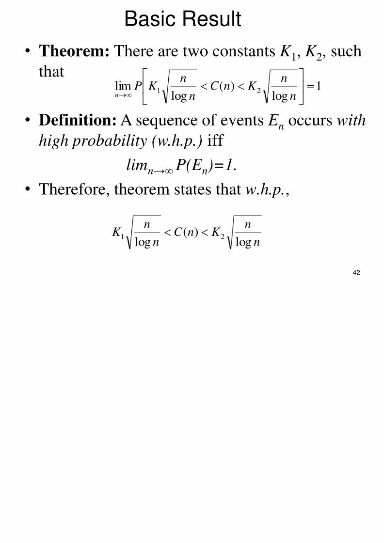
Basic Result

• Theorem: There are two constants K 1, K 2, such

that

• Definition: A sequence of events E n occurs with

high probability (w.h.p.) iff

limn→∞ P(E n)=1.

• Therefore, theorem states that w.h.p.,

42

1log

)(log

lim 21

n

nK nC

n

nK P

n

n

nK nC

n

nK

log)(

log21



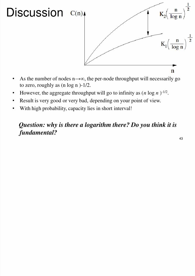
Discussion

• As the number of nodes n→∞, the per -node throughput will necessarily go

to zero, roughly as (n log n )-1/2.

• However, the aggregate throughput will go to infinity as (n log n )-1/2.

• Result is very good or very bad, depending on your point of view.

• With high probability, capacity lies in short interval!

Question: why is there a logarithm there? Do you think it is

fundamental?43



Sketch of Proofof Upper Bound:

44

1 P. Gupta and P. R. Kumar, „The Capacity of Wireless Networks,‟ IEEE Trans.On Information Theory, Vol. 46, No. 2, Mar. 2000, pp 388-404.

.1log

)(lim 2

n

nK nC Pn











• Assume protocol model with

max distance r(n)

• Each transmission consumes

an area around the receiver :

no other receiver can be in

the shaded disk.

• Number of simultaneous

transmissions T(n) multiplied by π ( Δr(n)/2)2 must be less

than area of networks (equal to 1):

T(n) ≤4/[πΔ2r(n)2].

• Therefore, at most 4W/[πΔ2(r(n))2] bps are transmitted by

the network at any given time. 45

Off d T ffi



Offered Traffic

• If every node creates traffic with rate λ( n),

aggregate created traffic is n λ(n).

• Each packet must be transmitted L/r(n) times,

where L is the average distance between

source and destination nodes.

• Offered traffic: n λ(n)L/r(n).

• Offered traffic must be less than achievable

traffic, so

46

)(

4)(

))((

4

)()(

222 nnr L

W n

nr

W

nr

Lnn

C i i R i



Connectivity Requirement

• We must have r(n)>[log n /n]1/2, otherwise

some of the nodes will be out of the range of

everyone else!

• Sketch of Proof:

• Setting the minimum value for r(n), we get the

upper bound. 47

n

i n ji

ii

n

i

i

X P X P

X PP

1 1

j

1

})isolatedareX,({})isolatedis({

}isolatedis {[]nodeisolatedanisthere[



Sketch of Proofof Lower Bound:

48

1 S. Toumpis and A. J. Goldsmith, Large Wireless Networks under Fading,Mobility, and Delay Constraints,‟ in IEEE Infocom 2004, Hong Kong, China,mar. 2004, vol.1, pp 609-619.

.1)(log

lim 1

nC

n

nK Pn

Proof Overview


http://papers/toumpis04b.pdf











Proof Overview• We know that many transmissions over small

distances are better than a few transmissions overa large distance.

• We will construct a scheme that uses the

principle.

– The basic complication is that node positions are

random.

• The per-node throughput of the scheme will be

better than K 1 /(n log n )1/2.

• The capacity is the supremum of all achievable

aggregate throughputs, so necessarily

C (n)>nK 1 /(n log n)1/2. 49

St 1 C ll



Step 1: CellLattice

• n nodes

• n/(k 1

log n) cells C 1

,C2,…

• m j nodes in cell C j

• On the average we have

k 1log n nodes per cell• In fact, as we saw:

P{k 1log n /2 ≤ m j ≤2k 1 log n for all j}→1, n→∞.

50

St 2 R ti



Step 2: Routing

• n nodes

• n/(k 1 log n) cells C 1 , C 2 ,…

• Nodes only transmit

to neighboring cells

• Hops per route

< 2(n/k 1 log n)1/2

• l j routes through cell C j

• W.h.p., for large enough k 2 ,

l j < (k 2 n log n)1/2 for all j

• Proof: again, Union Bound

51

Step 3: Time • Divide area in lattice of



Step 3: TimeDivision

• Divide area in lattice of

cells

• Divide cells in 9 regularsub-lattices

• Divide time frame in 9

slots• In each slot, a single

receiver in each cell of

the corresponding

sublattice receives data

from a single

transmitter.52



Throughput Calculation

• Guaranteed throughput per cell: T(n)=W/D.

• Routes per cell: l(n)<(k 2 n log n)1/2

• Guaranteed throughput per route (i.e., node):

λ(n)=T(n)/l(n)

• The capacity is the supremum of all achievable

throughputs, so

53

.log)(

)()( 1

n

nK

nl

nT nnC



Next: Some Extensions

1. Getting rid of the logarithm

2. Getting rid of the square root

3. Tougher traffic patterns

54



1. Getting Rid of the Logarithm1

• Question: do you think the logarithm is due

to the problem, or due to the solution?

• If we use the more realistic physical model, we

can dispense with the logarithm!

• But we need more advance mathematics.

• In fact, we need…

55

1 M. Franceschetti and O. Dousse and D. N. C. Tse and P. Thiran, „Closingthe Gap in the Capacity of Wireless Networks Via Percolation Theory,‟ in

IEEE Trans. On Information Theory, Vol. 53, No. 3, Mar. 2

http://papers/percolation.pdf











Percolation Theory

• Motivation: what is the rate with which water

trickles through the porous material?

56



TypicalResult

• Each node is connected with each of its neighbors, with

probability p.

• If p>0.5, an infinite connected cluster exists almost surely.

• If p<0.5, an infinite connected cluster does not exist,

almost surely. 57



Highway

System

• By reducing the size of the cells, we can have enough

of them full, so that a „highway system‟ is formed,consisting of around n1/2 horizontal and n1/2 vertical

highways.

• Using this construction, and the physical model, we

can get rid of the logarithm. 58



2. Getting Rid of the Square Root1,2

• Basic implicit assumption so far: nodes are not

allowed to cooperate in the coding/decoding

phase.

• If we use distributed MIMO, gains can be

impressive: Capacity increases faster than n1-ϵ ,

for any ϵ >0.

59

1 S. Aeron and V. Saligramma, „Wireless ad hoc networks: Strategies and scalinglaws for the fixed SNR regime,‟ IEEE Trans. Inf. Theory, vol. 53, no. 6, pp. 2044-2059, Jun. 20072 A. Özgür , O. Lévêque, and David N. C. Tse, ‘Hierarchical Cooperation Achieves

Optimal Capacity Scaling in Ad Hoc networks,’ in IEEE Trans. on Information

Theory, Vol. 53, No. 10, Oct. 2007, pp. 3549-3572.

T i k Hi hi l C ti

http://papers/aeron.pdf






http://papers/hierarchical_it.pdf





































Trick: Hierarchical Cooperation

• We divide nodes in hierarchical set of clusters.• Within same hierarchical level, nodes

communicate as follows:

1. Phase 1: Within each cluster, nodes distributetheir information to other nodes

2. Phase 2: Long Range MIMO transmissions

across many clusters3. Phase 3: Within each cluster, nodes distribute

information to recipients.

60

3 Asymmetric Traffic



3. Asymmetric Traffic • n source nodes, placed

uniformly and

independently.

• nd destination nodes

placed uniformly and

independently, where

the destination

exponent d ϵ (0,1).

• Each source node

chooses a random

destination node, so

there are around n1-d

sources for each

destination

• All sources require

end-to-end rate λ( n).61

Capacity of Asymmetric Networks



Capacity of Asymmetric Networks• Let the capacity C(n) =n sup λ(n)

• With probability going to 1 as the number of source nodesn→∞:

• To avoid the formation of bottlenecks in a network with n nodes, we need at least n 1/2 destinations.

• If destinations are costly and we want to minimize theirnumber, the network has a sweet spot:

– More than n 1/2 will not improve the capacity significantly

– Less than that, and bottlenecks start to form.

62

.2

1d0 ,log

,12

1 ,

)(log)(log

3

2 / 3

2 / 1

2

1

n

nK

d n

nK

nC nnK d

d

More Extensions



More Extensions• What happens if the network is three dimensional?

– Capacity increases like (n /log n)^2/3 – Gupta and P. R. Kumar, „Internets in the Sky: The Capacity of Three

Dimensional Wireless Networks,‟ Communications in Information andSystems, vol. 1, issue 1, pp. 33-49, Jan. 2001.

• What happens if there is fading?

– Performance of scheme that achieves lower bound is not reduced morethan a factor of log n, for many types of fading models

– S. Toumpis and A. J. Goldsmith, Large Wireless Networks under

Fading, Mobility, and Delay Constraints,‟ in IEEE Infocom 2004, HongKong, China, Mar. 2004, vol.1, pp 609-619.

• What happens if the bandwidth goes to infinity?

– Capacity increases like (n /log n)^2/3

– R. Negi and A. Rajeswaran, „Capacity of power constrained ad-hoc

networks,‟ in Proc. IEEE Infocom, Hong Kong, China, Mar. 2004.

63

More Extensions

http://papers/internet_sky.pdf






http://papers/negi.pdf






















More Extensions

• What happens when we have multicast traffic?

• What happens when traffic is localized?

• What happens when movement is constrainedor localized?

• Currently, Gupta/Kumar has 4602 citations, so

obviously no stone has been left unturned.

64



4. Asymptotic Capacity of

Networks with Mobile Nodes1

65

1 M. Grossglauser, D.N.C. Tse, „Mobility increases the capacity of ad hocwireless networks,‟ IEEE/ACM Transactions on Networking, Vol. 10, No. 4, pp.477-486, Aug. 2002.













Basic Idea

• Traditional thinking is that mobility has an adverse

effect on the capacity of networks.

– Overhead of routing protocols increases roughly linearly

with level of mobility.

• On the other hand, if we are willing to tolerate very

large delays, then we can take advantage of the

mobility to deliver our packets through physical

transport, rather than over the wireless channel.• Idea currently very hot (Delay Tolerant Networks).

66



Wishful Thinking (?)

• We know order O(n) simultaneous

transmissions are possible

• With immobile nodes, it is necessary to have

O(n1/2) such transmissions to reach destination

• With mobile nodes, if I find a way to only need

K , then total throughput will be O(n)/K=O(n)

• Grossglauser/Tse managed this, with K=2.

67

Network Model



Network Model

• Nodes placed in a disk of unit

area A = 1.

• Nodes move independently

of each other, according to

a stationary and ergodic

random process.

– Brownian motion, random walk are both acceptable.

• Each node has a random destination node (who is alsomoving).

• Nodes create traffic with a common rate λ(n) bps.

• Physical Transceiver Model 68

First Try (K 1)



First Try (K=1)• Since nodes are mobile, sources should wait

for destinations to come close, then transmit. – No relaying is needed.

• This idea is very simple, but does not perform

very well. In fact, any scheme that does notuse relaying can not do better than:

lim n →∞ P{ λ( n)=cn-1/(1+a/2) }=0 (1)

• Intuition: – It is best to transmit over small distances.

– At any given time, very few nodes are close to

their final destination. 69

Sketch of Proof



Sketch of Proof

• The following inequality holds:

• Where X j(i) is the destination of node X i, C is a constant,

and S is the set of successful transmissions.• Intuition: we cannot have too many transmissions over

too large distances, or SINR will be violated

somewhere.

• To exceed (1), we need more than cn-1/(1+a/2)

simultaneously successful transmissions.

• But then it is impossible to satisfy (2).

70

)2()(

Si

a

i ji C X X



Second try: Scheduling policy π (K=2)

• We slot time, and index slots by t .

• In each slot, each node transmits with

probability θ .

• Each transmits to its closest neighbor a packet

intended for its destination.

• There will be a lot of collisions, but by

previous result of Hajek et al., on the average

there will be φn successful transmissions.

71



But what do we transmit?

• In even slots, we transmit packets (to our

nearest neighbor) intended for our destination,

that he will give to our destination later on.

• In odd slots, we transmit packets intended forour nearest neighbor, that we received some

time in the past.

72

The book analogy



The book analogy

• Imagine a large number of people moving around in a

city.

• Each one carries a stack of books for a friend of his. The

stack is very high.

• Whenever I bump on any other person on the street: – I either give him a book for him to give to my buddy,

– or I give him a book that his buddy gave to me some time in

the past.

• Chances that I bump on my own buddy are negligible.

• Question: What is the average number of people that

their destinations are also nearest neighbors? This is

related to the famous hat (or wife) problem. 73

But Delay is Terrible!



But Delay is Terrible!

• Each node has to wait at the queue of the source

before it gets transmitted. – This delay is not very large.

• Each packet will also have to wait at the queue of

the relay: – With n nodes, the probability that any the destination will be

the closest neighbor of the receiver is only around 1/n.

– Therefore, on the average a packet will have to wait for n slots.

– The average delay per packet E[d]~ n.

• To summarize:

– The aggregate throughput is great: T(n) ~n packets at any time.

– The packet delay is terrible: E[d]~ n slots. 74

Throughput-Delay Tradeoff



Throughput Delay Tradeoff

• The scheme performs very well in terms of

throughput but very bad in terms of delay.• Can we exchange the two?

• One way to reduce delay, is to have more nodes act as

relays. – In the original scheme, only one node acts as the relay of the packet.

– If many nodes act as potential relays, statistically the packet will arrive

– faster.

– But for more nodes to act as relays, some sort of redundancy must be

used. This redundancy will inescapably reduce the throughput.

• Another way is to allow not two, but many hops from

the source to the destination.

• Next, we take a look at the various schemes that exist.75

1



First Scheme1

• Unrealistic mobility model

• Instead of a node giving the packet only to a single relay, it

successively gives na copies of the packet to na consecutive

relays, where the parameter a lies in (0, 1).

• All of the relays must be nearest neighbors.

• Delay increases like n1−a.

• Aggregate throughput increases like n1−a.

• We affect the delay-throughput tradeoff by modifying a.

76

1 M. Neely and E. Modiano, „Capacity and Delay Tradeoffs for Ad-HocMobile Networks,‟ in IEEE Trans. On Information Theory, Vol. 51, No. 6,June 2005.

Second scheme1

http://papers/neely.pdf













Second scheme

• Packets are duplicated, and at any given time, multiple relays

exist for the same packet.

• Instead of transmitting the packet multiple times (as in the first

scheme), nodes transmit their packets only once.

• But fewer transmissions are allowed at the same time, so

transmissions reach further away!

• The fewer the simultaneously allowed transmissions, the

smaller the aggregate throughput, but the smaller the delay.

• Aggregate throughput increases like na, 1/2 < a < 1.

• Delay increases like n2a−1.

77

1S. Toumpis and A. J. Goldsmith, Large Wireless Networks under Fading, Mobility,and Delay Constraints,‟ in IEEE Infocom 2004, Hong Kong, China, mar. 2004,vol.1, pp 609-619.

Third Scheme2













• Packets are not duplicated: at any given time, there is only one

copy of the packet in the network.• But: packets are allowed to make multiple hops to reach their

destination, once they are close enough.

• So this scheme is a combination of the schemes of Gupta/Kumar

and Grossglauser/Tse.• The more hops packets are allowed to make, the smaller the

aggregate throughput becomes, but the smaller the average delay

also becomes.

• Aggregate throughput increases like na

, where 1/2 < a < 1.• Delay increases like na−1/2

78

2A. El Gamal, J. Mamen, B. Prabhakar, D. Shah, „Throughput-DelayTrade-off in Wireless Networks,‟ in Proc. ACM/IEEE Infocom, Hong Kong,

China, Mar. 2004.

Tradeoff of

http://papers/mammen.pdf
















Tradeoff ofExponents

• Per node throughput λ(n) ~nt , packet delay d(n) ~nd .

• Differences in the curves are mostly due to different

assumptions on mobility models, and not so much on

any inherent advantage of any of the schemes. 79

The 2nd scheme



The 2 scheme,

in greater detail

• Nodes placed in square area.

• Node movements are

independent and uniform.

• For simplicity: – Within B secs, nodes do not move.

– Every S = NB secs, nodes get

perfectly reshuffled.

• (But results also hold for Brownian motion, various random walks,etc.)

• Experiment lasts for 2Nn D frames of duration B, where D is

integer, greater than 1.

• Physical Channel Model 80

C ll L i



Cell Lattice• n nodes.

• ( n1+d /k 1 log n)1/2 cells

C 1 ,C 2, . . .

• d is a design parameter,

with 0 < d < 1.• Let mij be the number of

nodes in cell C i, in frame j.

Then

E[mij] =(k 1n1−d log n)1/2.

• Lemma: With high probability, for all i, j,

k 2(n1−d log n)1/2 < mij < k 3(n

1−d log n)1/2

• Proof: Union bound.81

Time Division



Time Division

• Divide cells in 4 regular

sub-lattices.

• Divide frames in 4 slots

of duration B /4 .

• In each slot, a singlereceiver in each cell of the

corresponding sub-lattice

receives, from a single transmitter.• Lemma: With high probability, the SINRs of at least 50%

of the links at all slots are greater than k 4 log n.

• Proof: Straightforward.82

Tentative Frame Format



Tentative Frame Format

• By assumption, nodes are not moving for the

duration of a frame.

• After a frame passes, no nodes transmit

anything until nodes get perfectly reshuffled

again.83

Packet Transmissions



• Odd frames: Source-Relay Communication.

– Each node transmits a single packet, intended for its destination.

– Nodes that receive it will act as relays in subsequent even frames.

– Data rate used: R(n) = f R( k 5 log n).

– Packet duration: D(n) = k 6 n(d−1)/2 (log n)−3/2

– W. h. p., all nodes will get their chance to transmit a packet.

• Even frames: Relay-Destination Communication.

• Packets in the same cell with their destination are

delivered.

• W. h. p., all packets will have the time to be

transmitted.84

Final Frame Format



• Instead of waiting for node to be reshuffled,

we execute the same algorithm in parallel, N

times.85

Throughput and Delay Calculation



g p y

• Throughput calculation:

– Every 2B seconds, each node creates a packet. – Each packet has a size of R(n) × D(n) bits.

– Per-node throughput is λ(n) = R(n)× D(n) /2Β=k 6n(d−1)/2 (log n)−5/2

• Delay calculation:

– Each message is carried by around r(n) = (k 1n1−d log n)1/2 relays.

– These relays spread out in c(n) = ( n1+d k 1 log n)1/2 cells

– Probability that a packet will make it in a frame is only

r(n)/c(n) << 1.

– We need around c(n)/r(n) frames, or 2Nsc(n)/r(n) seconds.

– Lemma: W. h. p., all packets delivered with a delay smaller than

d max = (4Ns)nd .

86

Sanity Check



y

• All previous results involve serious

idealizations: – Number of nodes goes to zero

– Delay goes to infinity

– Throughput per node goes to zero – Size of buffers goes to infinity

– Node movements are independent, etc.

• So is it worth it? What do we get out of it?• Justification: these are all capacity results, which

express ultimate bounds, and abstract ways of

achieving them. 87



5. Capacity of Massive

Networks1

88

1 S. Toumpis, „Mother Nature knows Best: A survey of recent results onwireless networks based on Analogies with Physics,‟ Computer Networks, Vol52, Feb. 2008, pp. 360-383.

Underlying Theme


http://papers/mother_nature.pdf











Underlying Theme

• In the modeling phase we frequently arriveat equations / tradeoffs / concepts

occurring in nature

• Analogies with Physics should beexploited

1. We gain intuition

2. We end up with problems beaten to death!

• Especially true in wireless networks

– Spatial component

In this Part



In this PartA. “Packetoptics”

– Optimal route design using analogies with Optics

B. “Packetostatics”

– Optimal placement of nodes in wireless sensornetworks using analogies with Electrostatics

C. Cooperative Transmissions

D. Energy Efficient RoutingE. Load Balancing



A. “Packetoptics”1,2

1 P. Jacquet, „Geometry of Information Propagation in Massively Dense AdHoc Networks,‟ in Proc. ACM Mobihoc, May 2004, Roppongi, Japan, 157-

162.2 R. Catanuto, S. Toumpis, and Giacomo Morabito, “On AsymptoticallyOptimal Routing in Large Wireless Networks and Geometrical OpticsAnalogy,” Computer Networks, vol. 53, no. 11, pp. 1939-1955, July 2009.

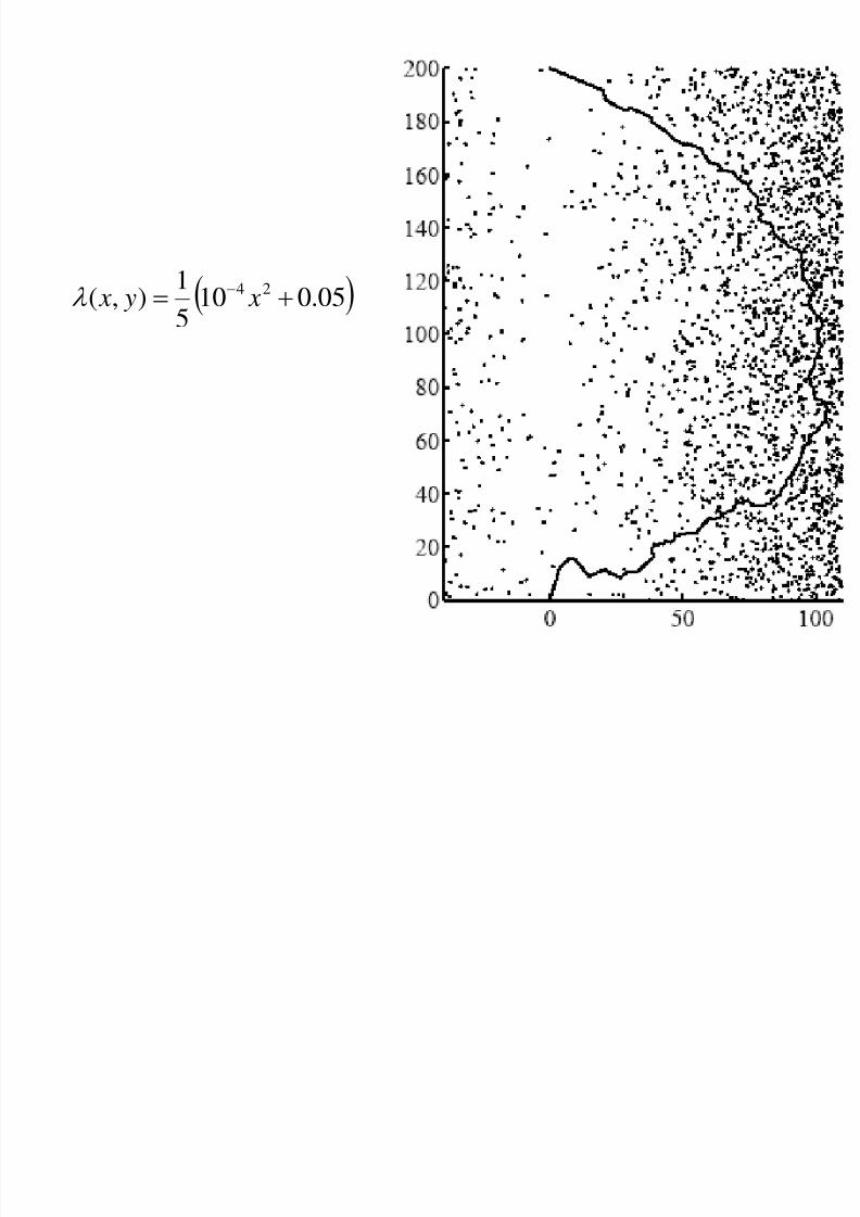
Appetizer

http://papers/jacquet.pdf





http://papers/catanuto.pdf



















pp

05.01030

1),( 24

x y x

Problem: Find route

between (0,0) and (0,200)with minimum cost.

Nodes distributed accordingto spatial Poisson process

Cost per hop increasesquadratically with hoplength:

.)( 2ad d c



05.010

10

1),( 24 x y x



05.0105

1),( 24

x y x



05.0102

1),(

24 x y x

Question: whathappens in the limit?

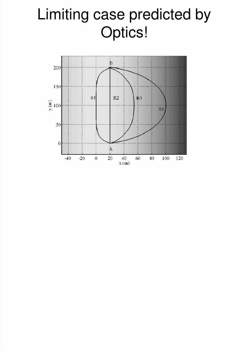
Limiting case predicted by



g p yOptics!

Macroscopic formulation



Macroscopic formulation

• Cost Function:

• Cost of route C that starts at A and ends at B:

• Problem: Find route from A to B that minimizes cost.

.),(

lim)(0

r

r

dcc

.)(][ B

A

C d c AB rr

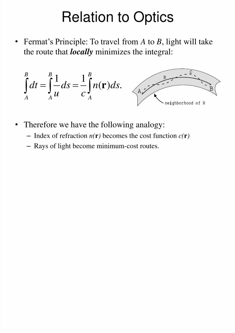
Relation to Optics



Relation to Optics

• Fermat‟s Principle: To travel from A to B, light will takethe route that locally minimizes the integral:

• Therefore we have the following analogy: – Index of refraction n(r) becomes the cost function c(r)

– Rays of light become minimum-cost routes.

.)(

11

B

A

B

A

B

Adsncdsudt r

Advantages of Optical Routing



Advantages of Optical Routing

• We can use the rich body of math thatalready exists in Optics for our setting.

– For example, we know that light satisfies the

following equations:

• We can use the intuition that already exists.

– For example, we know that rays of light bend

toward optically denser materials.

.||,)( nSnds

d n

ds

d

r

Various Choices for the Cost



Function

1. Promoting long hops

2. Promoting short hops

3. Promoting energy efficiency

4. Etc.

)()( rr c

)(

1)(

r

r

c

.,)(,0,)(

)),(()(

xconst x f x x f

f c rr

Choice of cost function very important!



R1: Jacquet, R2: Constant cost,

R3: Energy limited, R4: Bandwidth limited

Broadcast Routing



Broadcast RoutingThe optimal propagation of a packet resembles the

propagation of light emanating from a light source

Any practical gain by knowing the limit?



y p g y g

• With finite but many nodes, the optimum route is

hard to find• So let us find the optimum route in the

macroscopic limit, and use it to create a near

optimum route

What the Optics-Networking Analogy



does not tell us

• How does the source know the initial anglewith which the packet/ray should be launched?

• In some nonhomogeneous environments, there

are multiple rays connecting two points

– All of them local minimums

– One of them global minimum

Route



RouteDiscovery

• Basic idea: Nodes launch multiple rays

• Intersection points notify pairs of node



B. “Packetostatics”1,2

1 M. Kalantari, M. Shayman, „Energy Efficient Routing in Wireless Sensor

Networks,‟ in Proc. Conference on Information Sciences and Systems,Princeton University, NJ, Mar. 2004.2 S. Toumpis and L. Tassiulas, “Optimal Deployment of Large WirelessSensor Networks,” IEEE Trans. on Inform.Theory , vol. 52, no. 7, pp. 2935-2953, July 2006.

Setting

http://papers/kalantari.pdf







http://papers/toumpis06.pdf

































































































































Setting

• Wireless Sensor Network:

1. Sense the data at the source2. Transport the data from the sources to the sinks.

3. Deliver the data to the sinks.

• Problem: Minimize number of nodes needed

• What is the best placement for the wireless nodes? Whatis the traffic flow it induces?

Macroscopic View



p

• This problem is way too complicated to be

solved without proper abstractions

• Standard approach is based on microscopic

quantities: individual node placement,

individual link properties, etc.

• We can take a novel macroscopic approach,

using macroscopic quantities: node density,

data creation density, etc.

The Program



The Program1. Macroscopic quantities are connected with

each other through ‘constitutive laws’

– Microscopic considerations enter only through theformulation of these laws.

2. Approach opens gateway to new (or old,depending on how you look at it) Math:

– Calculus of Variations, Partial DifferentialEquations, Optics, Electrostatics, etc.

• Results are not as detailed as with standardapproach, but detailed enough to remainuseful

Macroscopic Quantities



Macroscopic Quantities• Node Density Function d(x,y), measured in nodes/m2.

– In area of size dA centered at (x,y) there are d(x,y)dA nodes• Information Density Function ρ(x,y), measured in

bps/m2.

– If ρ(x,y)>0 (<0), information is created (absorbed) with rate ρdA

over an area of size dA, centered at (x,y).• Traffic flow function T(x,y),

measured in bps/m.

– Traffic through incremental

line segment is |T(x,y)|dl.

What goes in must come out



What goes in, must come out• The net amount of information leaving a

surface A0 through its boundary B(A0), must

be equal to the net amount of information

created in that surface:

• Taking |A0|→0, we get the requirement:

)( 0 0

),()(ˆ

A B A

dS y xdss nT

(1)

y x

y x TTT

Special Case



Special Case1. Nodes only need to transfer data from

sources to sinks

1. They do not need to sense them at the sources

2. They do not need to deliver them to the sinks once

their location is reached

2. The traffic flow function and the node

density function are related by:

(2) ),(|),(| max y xd c y x T

Traffic must be irrotational



Traffic must be irrotational

• We must minimize the number of nodes

• If (2) is satisfied, then the traffic must beirrotational:

• Easy proof by contradiction.

.),( dA y xd N

.0

y x

x y TTT

„Packetostatics‟



Packetostatics• The traffic flow T and information density ρ must

satisfy:

• In free space, the electric field E and the charge

density ρ are uniquely determined by:

• Therefore, the optimal traffic distribution is the same

with the electric field when we substitute the sourcesand sinks with positive and negative charges!

.0 , TT

.0 , EE

Example: A point source and a lineari k



sink

Analogy is uncanny!



a ogy s u ca y

Electrostatics NetworksPotential differences Number of hops

Non-homogeneous

dielectrics

Non-homogeneous

propagation environmentsConductors Mobile sources and sinks

Thomson‟s theorem Source/Sink placement

optimizationIntersection of electric fieldlines and equipotentiallines

Node locations

Generalized Problem



Generalized Problem• Let

be the density of nodes needed to support thesensing/transport/delivery

• Optimization Problem:

• Minimization over all possible traffic flows T(x,y) that satisfythe constraint

• Standard tool for such problems: Calculus of Variations

|)),(|,,(),( y x y xG y xd T

).,(),( :subject to

)|),(,|,( :minimize 2

y x y x

dS y x y xG N

T

T

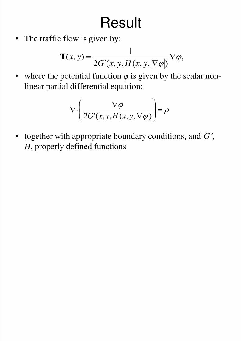
Result



Result• The traffic flow is given by:

• where the potential function φ is given by the scalar non-

linear partial differential equation:

• together with appropriate boundary conditions, and G’,

H , properly defined functions

,),,(,,(2

1),(

y x H y xG y xT

),,(,,(2 y x H y xG

Example: Gupta/Kumar physicall



layer

2

1

1max),(),( y xd c y x T

Example: Super Gupta/Kumar



Example: Super Gupta/Kumar

3

2


Example: Sub Gupta/Kumar



Example: Sub Gupta/Kumar

8

3


Example:



pMixedcase

below),(

above),(),(

8

3

1

3

2

1

max

y xd c

y xd c y xT

A final look at the optimization



problem

).,(),( :subject to

,)|),(,|,( :minimize 2

y x y x

dS y x y xG N

T

T

The integrant can have alternative

interpretations: delay, energy, etc. This is a problem in optimal

transportation



C. Cooperative

Transmissions1

1 B. Sirkeci-Mergen, A. Scaglione, and G. Mergen, “Asymptotic analysis ofmultistage cooperative broadcast in wireless networks,” IEEE/ACMTransactions on Networking, Vol. 14, Issue SI, June 2006, pp. 2531-2550

SettingT l l d l ft id f t i


http://papers/sirkeci.pdf













































































• Topology: source placed on left side of strip,

destination placed on right side of strip, relays

are placed in strip, Poisson distributed.

• Reception model: nodes susceptible to

thermal noise, power decays with distance as

pr (d)=kd -2 , reception successful if SINR>γ.

• Protocol: We slot time. In first slot, source

transmits. In i-th slot, everyone transmits if he

received for first time in previous slot.

Transmission powers add up at potential

receivers.



What the simulations say



y

• For sufficiently low threshold, a wave isformed that propagates along the strip. After a

while, wave achieves fixed width and goes on

for ever.• For high threshold, wave eventually dies out,

irrespective of how many nodes initially had

the packet.• Position of initial relays critical.

The massively densem ti



assumption

• Analysis very hard because of random

placement of nodes.

• Assumption: We have so many nodes, that

there is a node practically everywhere.

• Not interested in which node receives in i-th

slot.

• Interested in which region of space receives

in i-th slot.

The result



• Region that receives successfully in i-th slot is

vertical strip of width di=h(di-1).



D. Energy Efficient

Routing1

1 M. Kalantari, M. Shayman, „Energy Efficient Routing in Wireless SensorNetworks,‟ in Proc. Conference on Information Sciences and Systems,Princeton University, NJ, Mar. 2004.

Setting































































g

• A Wireless Sensor Network with multiplesources and a central sink.

• A very large number of nodes

– Modeled by node density function. – Not subject to optimization.

• Problem: Find routes from sources to the sink

that are energy efficient.• Intuition: Avoid concentration of traffic in any

given location.

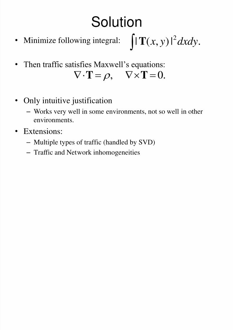
Solution



• Minimize following integral:

• Then traffic satisfies Maxwell‟s equations:

• Only intuitive justification

– Works very well in some environments, not so well in other

environments.

• Extensions:

– Multiple types of traffic (handled by SVD)

– Traffic and Network inhomogeneities

.|),(| 2dxdy y x

T

.0 , TT

Example



p



E. Load Balancing1

1 E. Hyytia and J. Virtamo, „On traffic load distribution and load balancing indense wireless multihop networks,‟ in EURASIP Journal on WirelessCommunications and Networking, Vol. 2007, No. 1, Jan. 2007.

Setting


http://papers/hyytia.pdf















































































g

• Until now, we supposed only one type of traffic, or at most a few.

• In general case, if there are n nodes, there will

be n(n-1) distinct traffics (and that ignoringmulticasting!)

• Macroscopic approach: Location r1 creates

traffic for location r2 with rate λ(r1 ,r2),measured in bps/m4.

Problem Formulation



• Set of all paths is P .

• Traffic through location r with direction θ has angular

flux Φ(P ,r,θ ), measured in bps/m/rad.

• Total volume that passes through location r is given by

scalar flux Φ(P ,r):

• Problem: Find optimal distribution of paths, so that

maximum traffic load is minimized:

.),,),2

0

d rr P P Φ( Φ(

).,maxargminopt rr

P P P

Φ(

Results



• Problem still very hard, even for highlysymmetric networks.

• Clever, sharp upper and lower bounds can be

found.• Insightful closed form expressions for angular

flux.

• Methods borrowed from the modeling of particle fluxes in Physics.

Conclusions



• New framework for studying problems, basedon macroscopic approach.

• Many optimization problems with a

pronounced spatial aspect can be handled.• Some detail is sacrificed, but solutions areinsightful.

• Math borrowed from Physics.

• Elephant in the room: we do not haveconvergence rates!

Parting CommentsA l i i h Ph i ll h



• Analogies with Physics are well worth

investigating• The field is particularly promising in wireless

networks due to their spatial aspect

• I showed you two examples of such analogies• Many more exit1

• Can you come up with others, in your own

research?

1A. Silva, E. Altman, P. Bernhard, M. Debbah, „Continuum Equilibria andGlobal Optimization for Routing in Dense Static Ad Hoc Networks,‟Computer Networks, In-Press, DOI: 10.1016/j.comnet.2009.10.019

Bibliography1. S. Aeron and V. Saligramma, „Wireless ad hoc networks: Strategies and scaling laws for the

fixed SNR regime,‟ IEEE Trans. Inf. Theory, vol. 53, no. 6, pp. 2044-2059, Jun. 2007.

http://papers/silva.pdf





















































































http://papers/mesh.pdf














































































g , y, , , pp ,

2. I. F. Akyildiz, X. Wang, and W. Wang, „Wireless Mesh Networks: a survey,‟ Computer

Networks, Vol. 47, 2005, pp. 445-487.

3. S. Burleigh, A. Hooke, L. Torgerson, K. Fall, V. Cerf, B. Durst, K. Scott and H. Weiss,„Delay-Tolerant Networking: An Approach to Interplanetary Internet,‟ IEEE

Communications Magazine, pp. 128-136, June 2003.

4. R. Catanuto, S. Toumpis, and Giacomo Morabito, “On Asymptotically Optimal Routing in

Large Wireless Networks and Geometrical Optics Analogy,” Computer Networks, vol. 53,

no. 11, pp. 1939-1955, July 2009.

5. A. El Gamal, J. Mamen, B. Prabhakar, D. Shah, „Throughput-Delay Trade-off in Wireless Networks,‟ in Proc. ACM/IEEE Infocom, Hong Kong, China, Mar. 2004.

6. K. Fall, „A Delay-Tolerant Architecture for Challenged Internets‟, ACM SIGCOMM, Aug.

2003, Karlsruhe, Germany.

7. M. Franceschetti and O. Dousse and D. N. C. Tse and P. Thiran, „Closing the Gap in the

Capacity of Wireless Networks Via Percolation Theory,‟ in IEEE Trans. On Information

Theory, Vol. 53, No. 3, Mar. 2007.8. M. Grossglauser, D.N.C. Tse, „Mobility increases the capacity of ad hoc wireless networks,‟

IEEE/ACM Transactions on Networking, Vol. 10, No. 4, pp. 477-486, Aug. 2002.

9. P. Gupta and P. R. Kumar, „The Capacity of Wireless Networks,‟ IEEE Trans. On

Information Theory, Vol. 46, No. 2, Mar. 2000, pp 388-404.

140

10. P. Gupta and P. R. Kumar, „Internets in the Sky: The Capacity of Three Dimensional

Wireless Networks,‟ Communications in Information and Systems, vol. 1, issue 1, pp. 33-

49, Jan. 2001.

11 B H j k d A K i h d R O L M i „O h C P b bili f L









































































































































































































































































































































































































































































































































































































































































































































11. B. Hajek and A. Krishna and R. O LaMaire, „On the Capture Probability for a Large

Number of Stations,‟ IEEE Trans. Communications, Vol. 45, No. 2, Feb. 1997.

12. E. Hyytia and J. Virtamo, „On traffic load distribution and load balancing in dense wirelessmultihop networks,‟ in EURASIP Journal on Wireless Communications and Networking,

Vol. 2007, No. 1, Jan. 2007.

13. P. Jacquet, „Geometry of Information Propagation in Massively Dense Ad Hoc Networks,‟in Proc. ACM Mobihoc, May 2004, Roppongi, Japan, 157-162.

14. P. Juang, H. Oki, Y. Wang, M. Martonosi, L.-S. Peh, and D. Rubenstein, „Energy-Efficient

Computing for Wildlife Tracking: Design Tradeoffs and Early Experiences with ZebraNet,‟in Proc. ACM ASPLOS 2002.

15. M. Kalantari, M. Shayman, „Energy Efficient Routing in Wireless Sensor Networks,‟ in

Proc. Conference on Information Sciences and Systems, Princeton University, NJ, Mar.

2004.

16. R. Negi and A. Rajeswaran, „Capacity of power constrained ad-hoc networks,‟ in Proc.

IEEE Infocom, Hong Kong, China, Mar. 2004.

17. M. Neely and E. Modiano, „Capacity and Delay Tradeoffs for Ad-Hoc Mobile Networks,‟ in

IEEE Trans. On Information Theory, Vol. 51, No. 6, June 2005.

18. A. Özgür , O. Lévêque , and David N. C. Tse , ‘Hierarchical Cooperation Achieves Optimal

Capacity Scaling in Ad Hoc networks,’ in IEEE Trans. On Information Theory, Vol. 53, No.

10, Oct. 2007, pp. 3549-3572.

141

19. A. Silva, E. Altman, P. Bernhard, M. Debbah, „Continuum Equilibria and GlobalOptimization for Routing in Dense Static Ad Hoc Networks,‟ Computer Networks, In-Press,

DOI: 10.1016/j.comnet.2009.10.019

20. B. Sirkeci-Mergen, A. Scaglione, and G. Mergen, “Asymptotic analysis of multistage

i b d i i l k ” IEEE/ACM T i N ki V l























































































































































































































































































































































































































































































































































































































































































































cooperative broadcast in wireless networks,” IEEE/ACM Transactions on Networking, Vol.

14, Issue SI, June 2006, pp. 2531-2550.

21. J. A. Silvester and L. Kleinrick, „On the Capacity of Multihop Slotted ALOHA Networkswith Regular Structure,‟ in IEEE Trans. On Communications, Vol. COM-31, No. 8, Aug.

1983, pp. 974-982.

22. G. Sharma, R. Mazumdar, N. B. Shroff, “Delay and Capacity trade-offs in mobile ad hoc

Networks,‟ in IEEE.ACM Trans. On Networking, Vol. 15, No. 5, Oct. 2007, pp. 981-992.

23. T. Small and Z. J. Haas, „The Shared Wireless Infostation Model – A New Ad Hoc

Networking Paradigm (or where there is a Whale, there is a Way),‟ in Proc. ACM Mobihoc

2003, June 2003, Annapolis, MD.

24. S. Toumpis, „Capacity Bounds for Three Classes of Wireless Networks: Asymmetric,

Cluster, and Hybrid,‟ in Proc. ACM Mobihoc, May 2004, Roppongi, Japan.

25. S. Toumpis, „Mother Nature knows Best: A survey of recent results on wireless networks

based on Analogies with Physics,‟ Computer Networks, Vol 52, Feb. 2008, pp. 360-383.

26. S. Toumpis and A. J. Goldsmith, Large Wireless Networks under Fading, Mobility, and

Delay Constraints,‟ in IEEE Infocom 2004, Hong Kong, China, mar. 2004, vol.1, pp 609-

619.
















































































































































































































































































































































































































































































































Documents

Wireless Network Capacity