Embed Size (px)
Citation preview
Wireless Network Design: Wireless Network Design: Implicit Loss Models, PHY Feedback, Implicit Loss Models, PHY Feedback,
Performance SensitivitiesPerformance Sensitivities
John S. Baras
Institute for Systems Research
Department of Electrical and Computer Engineering
Department bof Computer Science
Fischell Department of Bioengineering
University of Maryland College Park
USC Workshop on Wireless NetworksLos Angeles, May 20-21, 2008
Maryland Hybrid Networks Center Maryland Hybrid Networks Center (HyNet)(HyNet)
1Copyright © John S. Baras 2008
Network Science - 1Network Science - 1• What is a Network?
– In several fields or contexts: social, economic, communication, sensor, biological, physics and materials
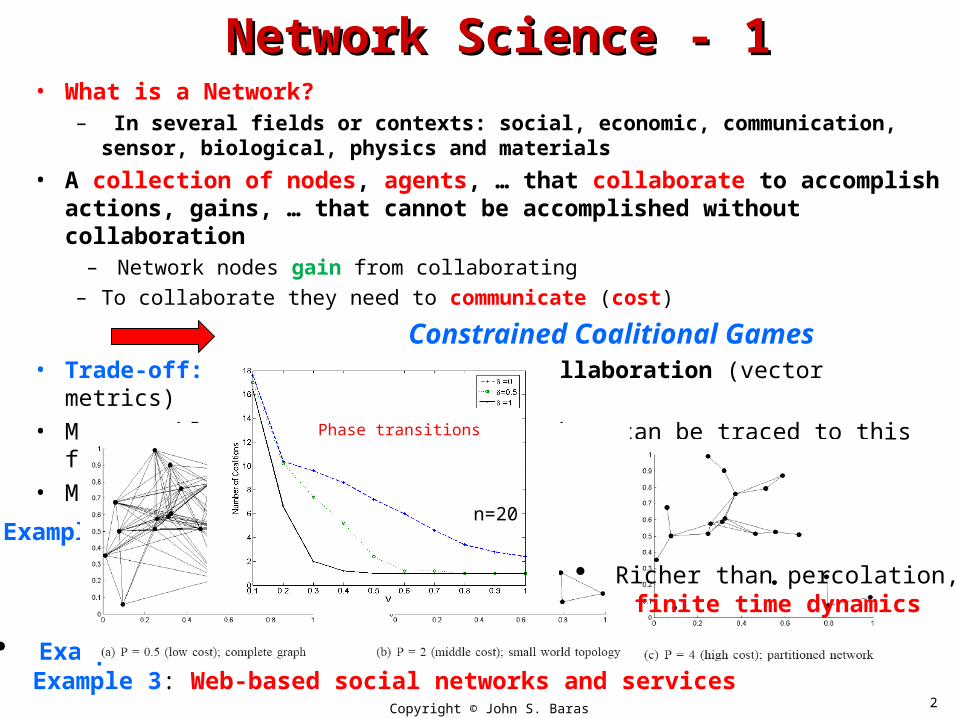
• A collection of nodes, agents, … that collaborate to accomplish actions, gains, … that cannot be accomplished without collaboration
– Network nodes gain from collaborating
– To collaborate they need to communicate (cost)
Constrained Coalitional Games • Trade-off: gain from vs cost of collaboration (vector metrics)• Many problems in networks (all fields), can be traced to this fundamental
trade off • Most significant principle for autonomic networks
Copyright © John S. Baras 2008 2
Example 1: Network Formation -- Effects on Topology
Example 2: Collaborative communications Example 3: Web-based social networks and services
Richer than percolation, finite time dynamics
Phase transitions
n=20
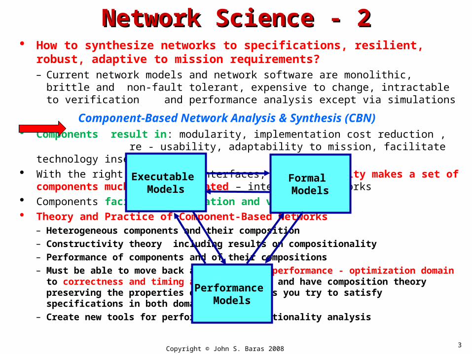
How to synthesize networks to specifications, resilient, robust, adaptive to mission requirements?– Current network models and network software are monolithic, brittle and non-
fault tolerant, expensive to change, intractable to verification and performance analysis except via simulations
Component-Based Network Analysis & Synthesis (CBN) Components result in: modularity, implementation cost reduction ,
re - usability, adaptability to mission, facilitate technology insertion With the right (powerful) interfaces, programmability makes a set of
components much more integrated – intelligent networks Components facilitate validation and verification Theory and Practice of Component-Based Networks
– Heterogeneous components and their composition– Constructivity theory including results on compositionality– Performance of components and of their compositions – Must be able to move back and forth form performance - optimization domain to
correctness and timing analysis domain and have composition theory preserving the properties of components as you try to satisfy specifications in both domains
– Create new tools for performance and functionality analysis
Copyright © John S. Baras 2008 3
Network Science - 2Network Science - 2
Executable Models
Performance Models
Formal Models
Qo
S D
rive
n D
esig
n
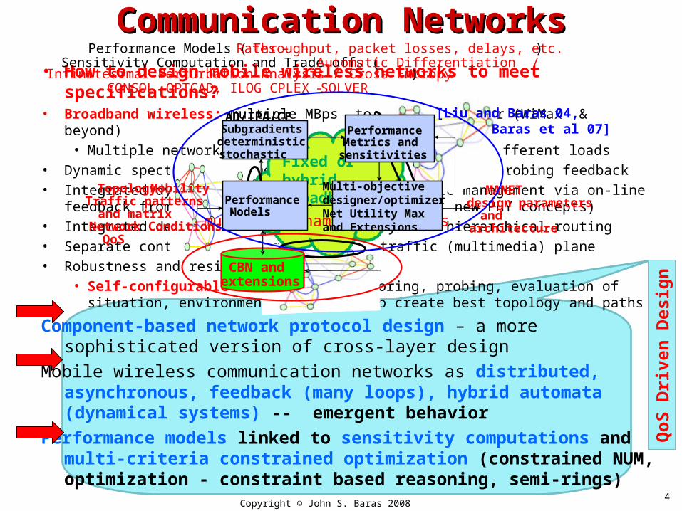
• How to design mobile wireless networks to meet specifications?• Broadband wireless: multiple MBps to the mobile user (WiMax & beyond)
• Multiple networks-multiple routes optimized for different loads• Dynamic spectrum management and allocation based on probing feedback • Integrated dynamic coordination of interference management via on-line feedback from
PHY (MIMO, directional antennas, new PHY concepts)• Integrated design of adaptive MAC and dynamic hierarchical routing• Separate control-signaling plane from traffic (multimedia) plane• Robustness and resiliency
• Self-configurable networks -- Monitoring, probing, evaluation of situation, environment and demand to create best topology and paths
Component-based network protocol design – a more sophisticated version of cross-layer design
Mobile wireless communication networks as distributed, asynchronous, feedback (many loops), hybrid automata (dynamical systems) -- emergent behavior
Performance models linked to sensitivity computations and multi-criteria constrained optimization (constrained NUM, optimization - constraint based reasoning, semi-rings)
Copyright © John S. Baras 2008 4
Communication NetworksCommunication Networks
Fixed or hybrid broadband
multiple dynamic interfaces
CBN and extensions
Performance Models ( Rates – Throughput, packet losses, delays, etc. )Sensitivity Computation and Trade offs ( Automatic Differentiation / Infinitesimal Perturbation Analysis / Cross Entropy ) CONSOL -OPTCAD, ILOG CPLEX -SOLVER
Topology-MobilityTraffic patternsand matrix
Network ConditionsQoS
MANET design parameters and architecture
Performance Models
Multi-objectivedesigner/optimizerNet Utility Max and Extensions
AD/IPA/CE Subgradientsdeterministicstochastic
Performance Metrics and sensitivities
[Liu and Baras 04, Baras et al 07]
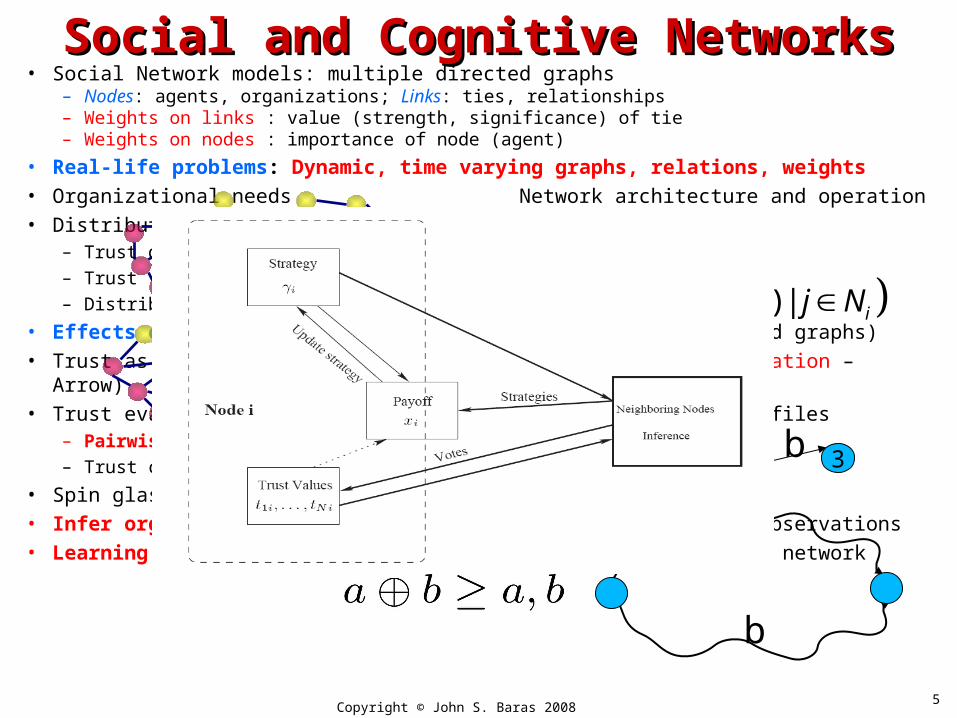
Social and Cognitive NetworksSocial and Cognitive Networks• Social Network models: multiple directed graphs
– Nodes: agents, organizations; Links: ties, relationships– Weights on links : value (strength, significance) of tie– Weights on nodes : importance of node (agent)
• Real-life problems: Dynamic, time varying graphs, relations, weights• Organizational needs Network architecture and operation • Distributed trust management systems in autonomic networks
– Trust document distribution, trust metrics, trust management– Trust (and Mistrust) spreading, dynamics, voting, policies– Distributed, high integrity reputation and recommender systems
• Effects of topology on convergence (efficiency -- small world graphs)• Trust as incentive for collaboration (lubricant for collaboration – Arrow)• Trust evaluation: direct and indirect ways; reputations, profiles
– Pairwise games on graphs with players of many types– Trust computation via linear iterations in ordered semirings
• Spin glasses (from statistical physics), phase transitions• Infer organizational structure from partial communications observations • Learning on graphs and network games: behavior, adversaries, network
Copyright © John S. Baras 2008 5
2 31 a b
b
a
ˆ( 1) , ( ) |i ji j is k f J s k j N
Implicit Loss Models and ADImplicit Loss Models and AD
• Simple approximate loss network model that couples the physical, MAC and routing layers to estimate the total network throughput
• Optimization framework using Automatic Differentiation (AD) for sensitivity analysis; applications to robustness, to maximizing throughput w.r.t. routing parameters, etc.
• Substantial extensions to include multiple paths, non-saturated flows, hidden nodes, scheduling, MAC/PHY failures
6Copyright © John S. Baras 2008
MotivationMotivation
• Discrete packet simulation tools (e.g. ns2, OPNET) take too much time even for simple network configurations and light traffic
• Our objective: to develop models that estimate the performance of a MANET fast. Design for predicatble performance bounds (specifications)
• Inputs: network topology (could be time varying), neighborhood relations (channel conditions), traffic demand (source-destination pairs, data rates, number of paths).
7Copyright © John S. Baras 2008
ApproachApproach
• We define two sets of equations:– The first set describes the specific MAC and PHY models we
consider and expresses the loss parameters and the outgoing rate of a link in terms of the incoming rates and the interference from neighboring links
– The second set describes the relations between flows and the scheduling parameters at each node
• Two sets are coupled iteratively, on the entire network, in a fixed point setting till they converge to a consistent solution
• Then, we evaluate the robustness of the solution using AD:– AD provides the partial derivatives of the performance metric
(throughput) w.r.t. design parameters (e.g. routing probabilities)– Using these partial derivatives with the gradient projection
method we solve for the design parameters that maximize the total network throughput
8Copyright © John S. Baras 2008
PreliminariesPreliminaries
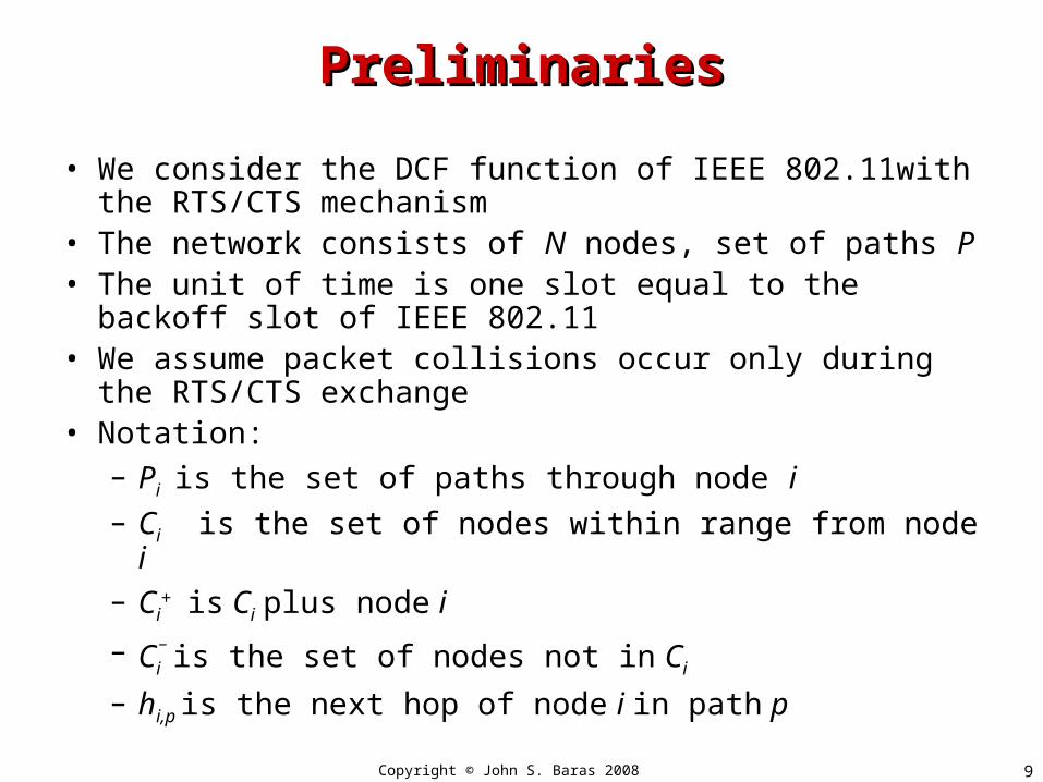
• We consider the DCF function of IEEE 802.11with the RTS/CTS mechanism
• The network consists of N nodes, set of paths P• The unit of time is one slot equal to the backoff slot of
IEEE 802.11• We assume packet collisions occur only during the
RTS/CTS exchange• Notation:
– Pi is the set of paths through node i– Ci is the set of nodes within range from node i– Ci
+ is Ci plus node i
– Ci
_ is the set of nodes not in Ci
– hi,p is the next hop of node i in path p9Copyright © John S. Baras 2008

Prior Related WorkPrior Related Work
• Bianchi [2000]
• Kumar, Altman, et al [2005]
• Garetto, Salonidis, Knightly [2006]
• Medepalli, Tobagi [2006]
• Hira, et al [2006]
• Liu, Baras [2004]
10Copyright © John S. Baras 2008
PHY/MAC ParametersPHY/MAC Parameters
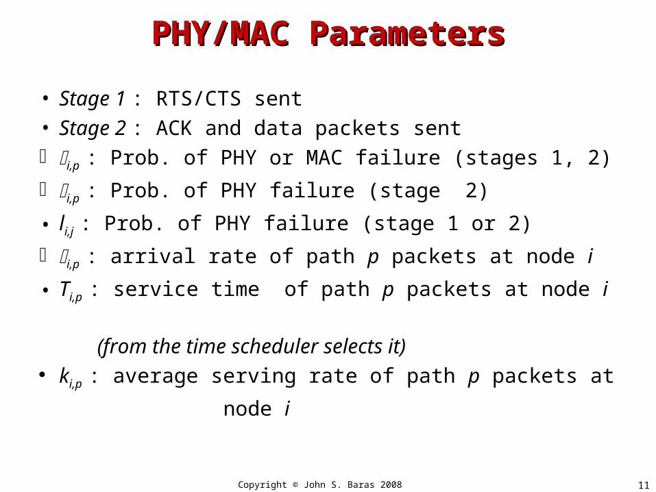
• Stage 1 : RTS/CTS sent• Stage 2 : ACK and data packets sent i,p : Prob. of PHY or MAC failure (stages 1, 2)
i,p : Prob. of PHY failure (stage 2)
• li,j : Prob. of PHY failure (stage 1 or 2)
i,p : arrival rate of path p packets at node i
• Ti,p : service time of path p packets at node i
(from the time scheduler selects it) ki,p : average serving rate of path p packets at
node i11Copyright © John S. Baras 2008
Scheduler CoefficientsScheduler Coefficients
, , '
, '', , '
,,
,
, '
, '' , '
, if E( ) 1 (1 ) (1 )
(1 ), otherwise
E( )(1 )
i
i
i p i p
i pm mp Pi p i p
i pi p m
i p
i p
i pmp P i p
T
k
T
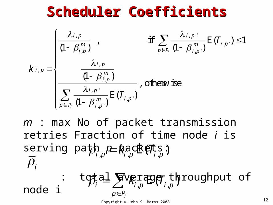
m : max No of packet transmission retries Fraction of time node i is serving path p packets:
: total average throughput of node i, , ,E( )i p i p i pk T
i
, ,E( )i
i i p i pp P
k T
12Copyright © John S. Baras 2008
Collision and Hidden Collision and Hidden Nodes Modeling (1)Nodes Modeling (1)
,'',
, , ,
2(1 )
(1 2 ) ( 1)(1 (2 ) )i p
i p Li p i p i p
aW W
,
, , , ,
, ,
, , , , ', , ',' '
1 (1 )(1 ) (1 ) (1 ) i p
i p i p i p i p
j jh i h ii p i p
V
i p i h h i j p h j p hp P p Pj C C j C C
l a a
'', , , , ,(1 )i p j i p i j i pa a
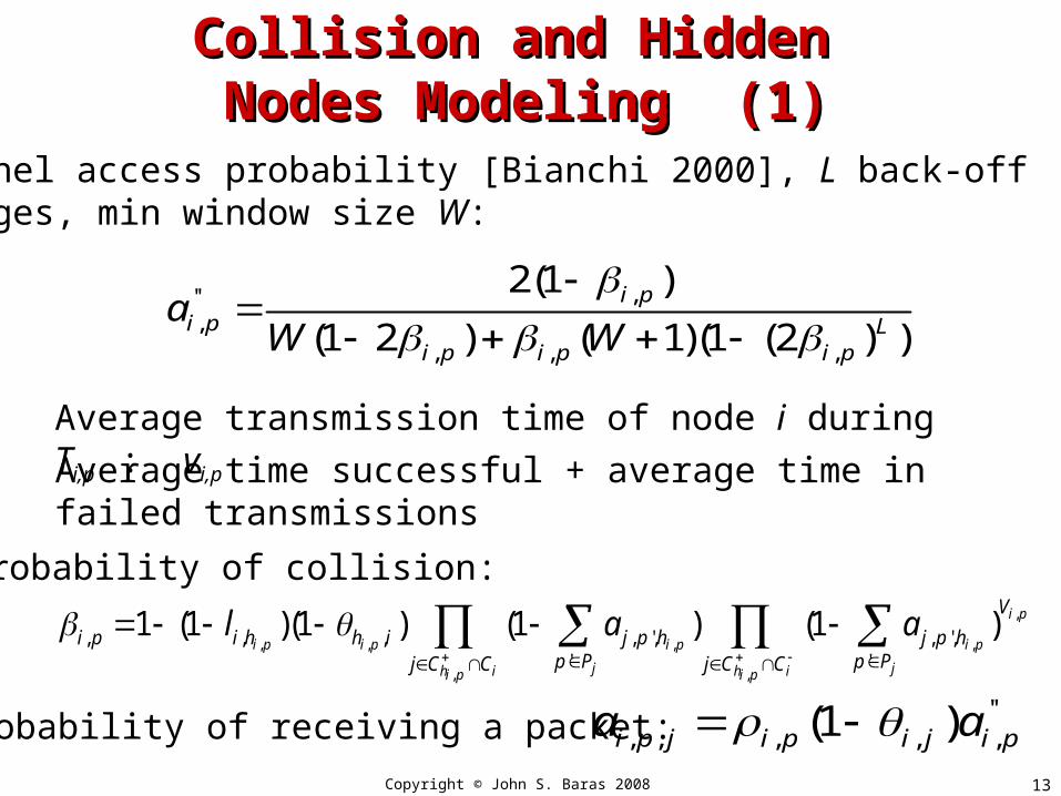
Channel access probability [Bianchi 2000], L back-off stages, min window size W:
Probability of collision:
Probability of receiving a packet:
Average transmission time of node i during Ti,p : vi,p
Average time successful + average time in failed transmissions
13Copyright © John S. Baras 2008
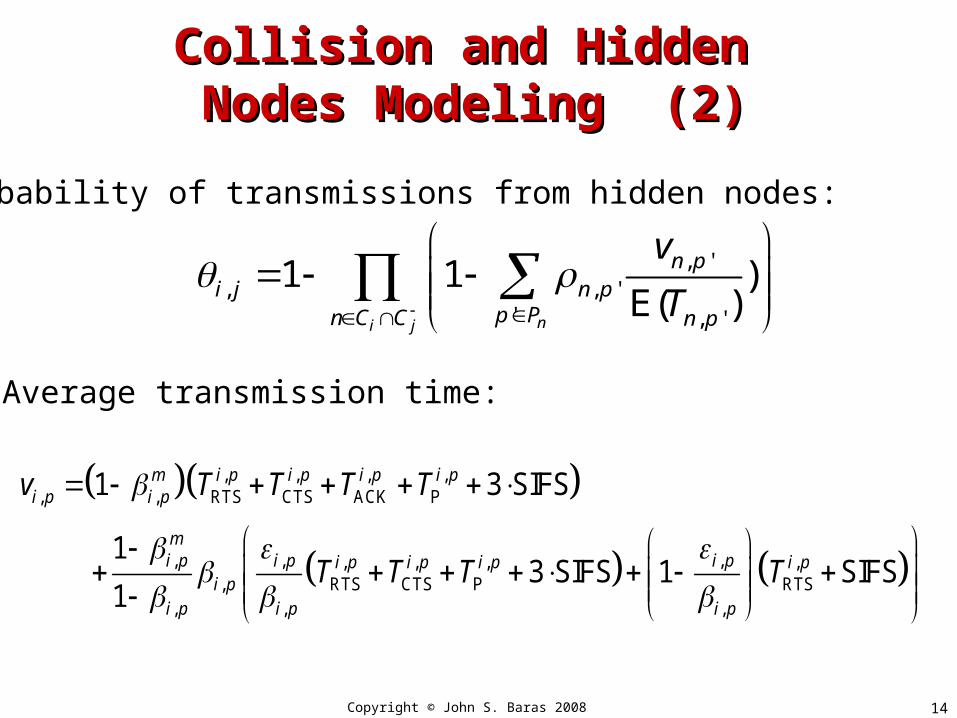
Collision and Hidden Collision and Hidden Nodes Modeling (2)Nodes Modeling (2)
, ', , '
' , '
1 1 )E( )
ni j
n pi j n p
p Pn C C n p
v
T
Probability of transmissions from hidden nodes:
Average transmission time:
, , , ,, , RTS CTS ACK P
, , ,, , , ,, RTS CTS P RTS
, , ,
1 3 SIFS
1 3 SIFS 1 SIFS
1
m i p i p i p i pi p i p
mi p i p i pi p i p i p i p
i pi p i p i p
v T T T T
T T T T
14Copyright © John S. Baras 2008
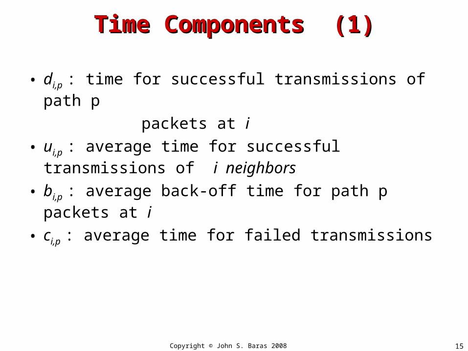
• di,p : time for successful transmissions of path p
packets at i
• ui,p : average time for successful transmissions of i neighbors
• bi,p : average back-off time for path p packets at i
• ci,p : average time for failed transmissions
Time Components (1)Time Components (1)
15Copyright © John S. Baras 2008
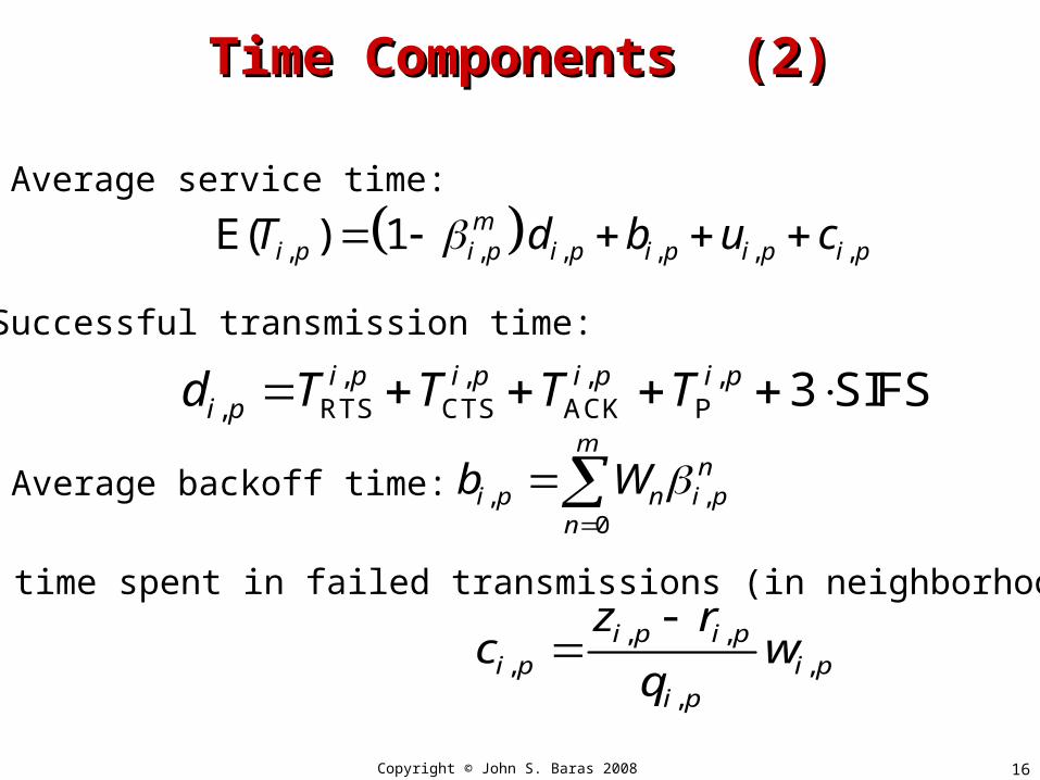
Time Components (2)Time Components (2)
, , , , , ,E( ) 1 mi p i p i p i p i p i pT d b u c
, , , ,, RTS CTS ACK P 3 SIFSi p i p i p i pi pd T T T T
, ,0
mn
i p n i pn
b W
Average service time:
Successful transmission time:
Average backoff time:
Average time spent in failed transmissions (in neighborhood of i ):
, ,, ,
,
i p i pi p i p
i p
z rc w
q
16Copyright © John S. Baras 2008
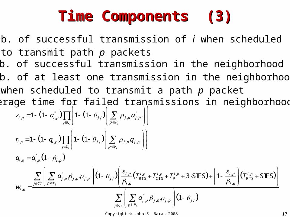
Time Components (3)Time Components (3)
'' '', , , , ' , '
'
, , , , ' , ''
'', , ,
,'' ,, ' , ' , ' , RTS
' ,
,
1 1 1 1
1 1 1 1
1
1
ji
ji
ji
i p i p j i j p j pp Pj C
i p i p j i j p j pp Pj C
i p i p i p
i p i pj p j p j p j i
p Pj C i p
i p
z a a
r q q
q a
a T
w
,, , ,CTS P RTS
,
'', ' , ' , ' ,
'
3 SIFS 1 SIFS
1ji
i pi p i p i p
i p
j p j p j p j ip Pj C
T T T
a
qi,p: Prob. of successful transmission of i when scheduled to transmit path p packetsri,p: Prob. of successful transmission in the neighborhood of izi,p: Prob. of at least one transmission in the neighborhood of i , when scheduled to transmit a path p packetwi,p: average time for failed transmissions in neighborhood of i
17Copyright © John S. Baras 2008
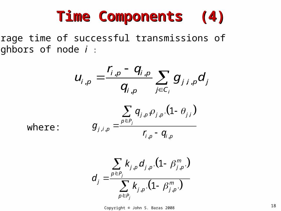
Time Components (4)Time Components (4)
, ,, , ,
, i
i p i pi p j i p j
j Ci p
r qu g d
q
Average time of successful transmissions of neighbors of node i :
where:
, ' , ' ,'
, ,, ,
, ' , ' , ''
, ' , ''
1
1
1
j
j
j
j p j p j ip P
j i pi p i p
mj p j p j p
p P
j mj p j p
p P
q
gr q
k d
dk
18Copyright © John S. Baras 2008
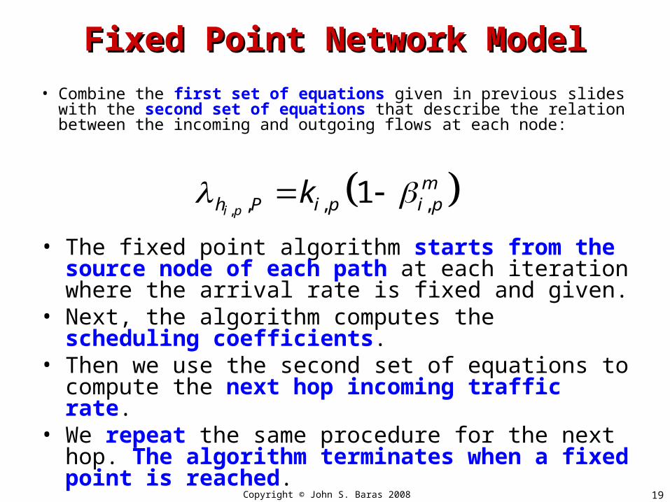
Fixed Point Network ModelFixed Point Network Model
• Combine the first set of equations given in previous slides with the second set of equations that describe the relation between the incoming and outgoing flows at each node:
, , , ,1i p
mh P i p i pk
• The fixed point algorithm starts from the source node of each path at each iteration where the arrival rate is fixed and given.
• Next, the algorithm computes the scheduling coefficients.
• Then we use the second set of equations to compute the next hop incoming traffic rate.
• We repeat the same procedure for the next hop. The algorithm terminates when a fixed point is reached.
19Copyright © John S. Baras 2008
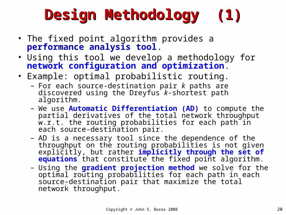
Design Methodology (1)Design Methodology (1)
• The fixed point algorithm provides a performance analysis tool.
• Using this tool we develop a methodology for network configuration and optimization.
• Example: optimal probabilistic routing.– For each source-destination pair k paths are discovered using
the Dreyfus k-shortest path algorithm.– We use Automatic Differentiation (AD) to compute the partial
derivatives of the total network throughput w.r.t. the routing probabilities for each path in each source-destination pair.
– AD is a necessary tool since the dependence of the throughput on the routing probabilities is not given explicitly, but rather implicitly through the set of equations that constitute the fixed point algorithm.
– Using the gradient projection method we solve for the optimal routing probabilities for each path in each source-destination pair that maximize the total network throughput.
20Copyright © John S. Baras 2008
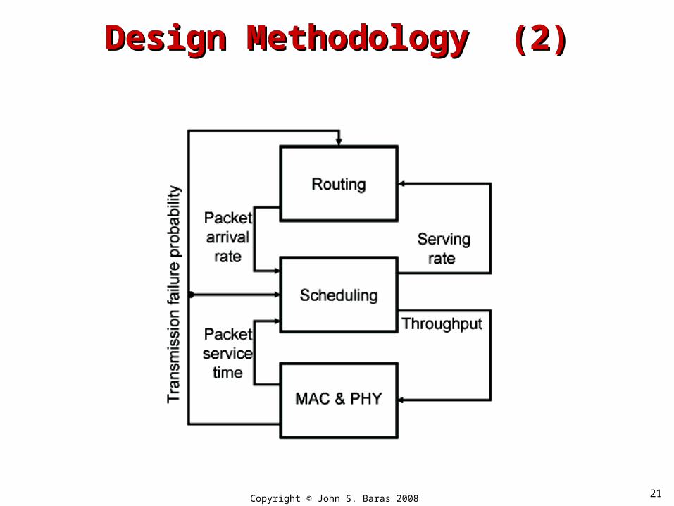
Design Methodology (2)Design Methodology (2)
21Copyright © John S. Baras 2008
Automatic Differentiation (AD)Automatic Differentiation (AD)
• Goal: maximize network throughput w.r.t. the routing probabilities.
• There is no analytic expression that gives the throughput as a function of the routing probabilities; instead, the code that computes the fixed point for the set of equations presented above provides such description (implicitly).
• Thus, AD is necessary: it repeatedly applies the chain rule to combine the local partial derivatives of each executed operator in the code.
• The optimization method used is Gradient Projection.
22Copyright © John S. Baras 2008
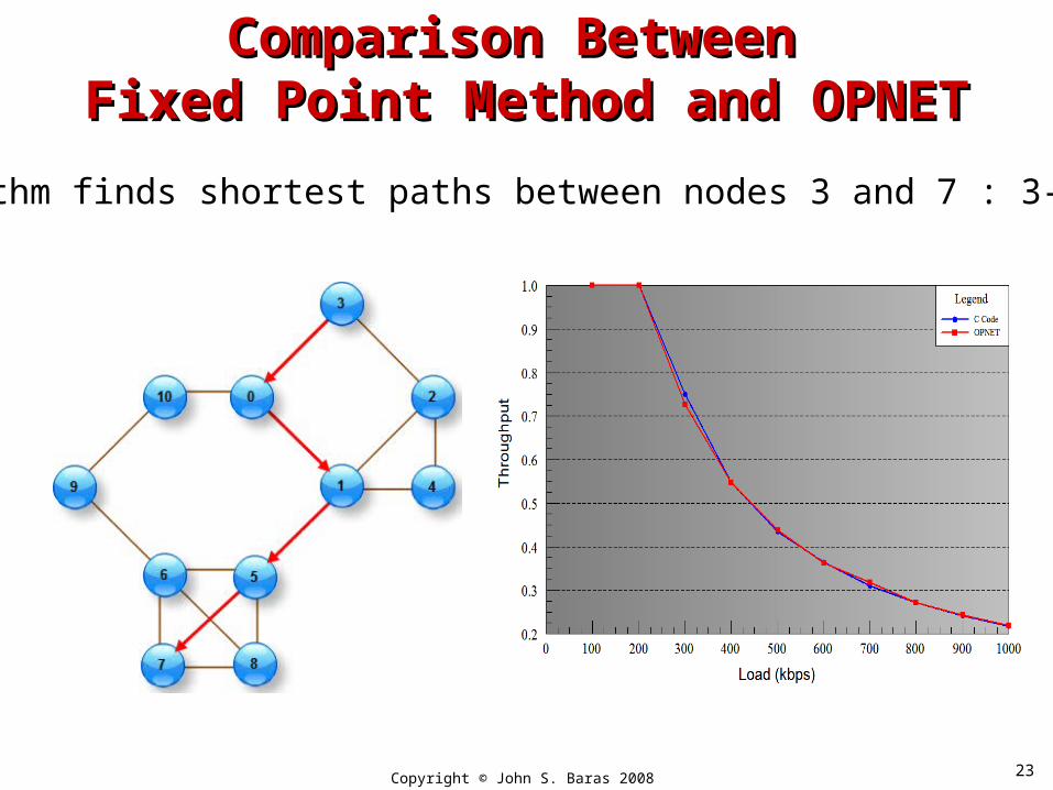
Comparison Between Comparison Between Fixed Point Method and OPNETFixed Point Method and OPNET
Algorithm finds shortest paths between nodes 3 and 7 : 3-0-1-5-7
23Copyright © John S. Baras 2008
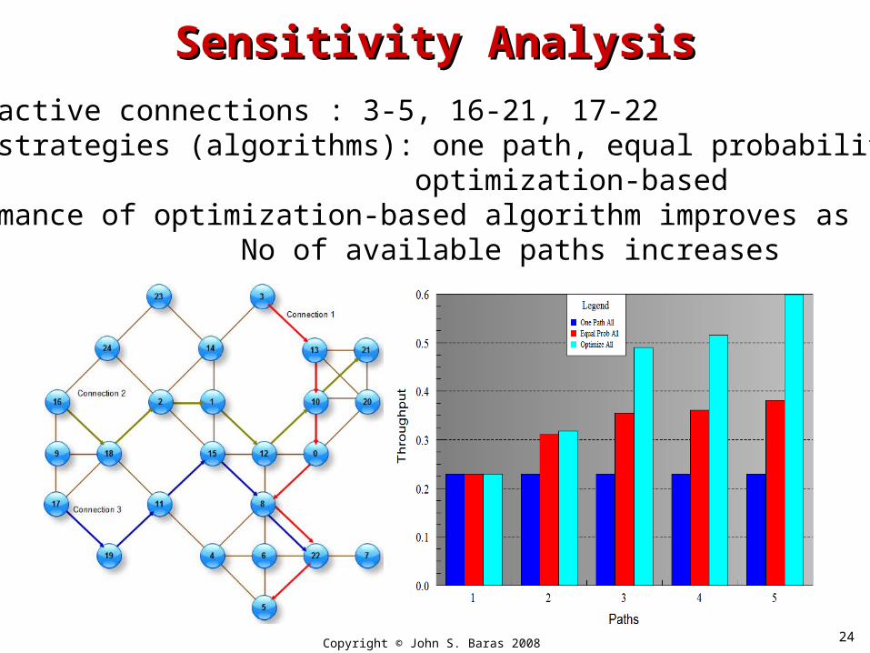
Sensitivity AnalysisSensitivity Analysis
Three active connections : 3-5, 16-21, 17-22Three strategies (algorithms): one path, equal probabilities,
optimization-basedPerformance of optimization-based algorithm improves as
No of available paths increases
24Copyright © John S. Baras 2008
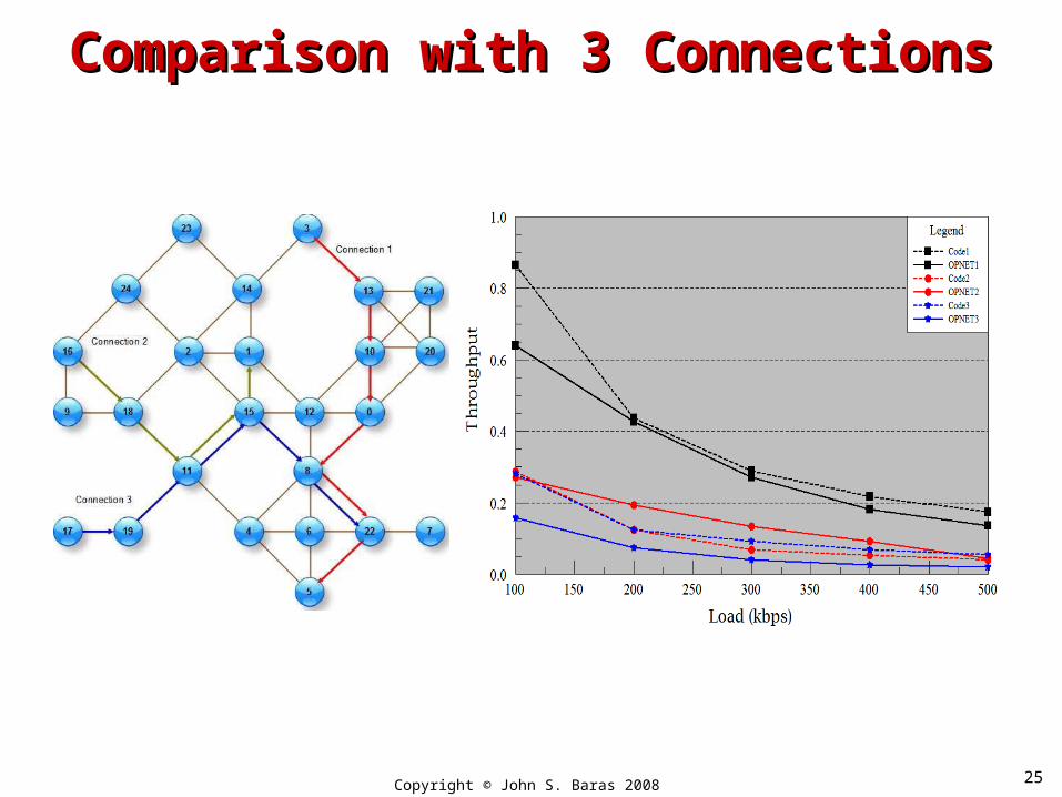
Comparison with 3 ConnectionsComparison with 3 Connections
25Copyright © John S. Baras 2008
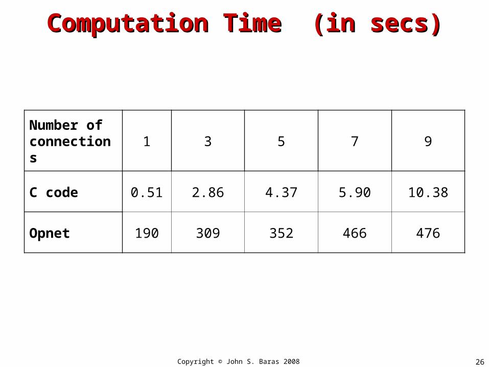
Computation Time (in secs)Computation Time (in secs)
Number of connections
1 3 5 7 9
C code 0.51 2.86 4.37 5.90 10.38
Opnet 190 309 352 466 476
26Copyright © John S. Baras 2008
27
CBN -- Beyond ModularityCBN -- Beyond Modularity
• With the right interfaces, programmability makes the set of components much more integrated – intelligent networks
• Like in networked embedded systems• Insisting on orthogonallity of concerns for
components is not correct• Components will interact – We need to control
the interaction through integration – possible only with new more powerful interfaces
5/30/2007 28
CBR -- Performance Metrics for CBR -- Performance Metrics for
Routing ComponentsRouting Components • Component selection: how to evaluate and
compare different components under different environments (Network topology, Traffic scenario, Mobility profile, Link states)?
• Meaningful Component Metrics are crucial for components performance evaluation, comparison, selection
• Finer metrics than System Performance Metrics (Latency, Throughput, Packet Loss Ratio)
• Statistics can be collected during network activities
5/30/2007 29
CBR -- Routing Protocol Metrics CBR -- Routing Protocol Metrics vsvs Component Derivative Metrics Component Derivative Metrics
• Goal: Evaluate the components against relevant metrics that will not only differentiate the various components but will also relate the performance of the component with the routing protocol performance.
Also link to other layer metrics (e.g. MAC)
• Derivative Metrics: • Route selection latency (sec)• Route selection overhead (packets/sec)• Number of routes found and ranking• Quality of the routes (stability, E2E rate delay loss)
30
Modeling and Performance of Modeling and Performance of MANET Routing (and MANET Routing (and
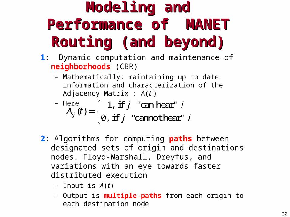
beyond)beyond)1: Dynamic computation and maintenance of
neighborhoods (CBR)– Mathematically: maintaining up to date information and
characterization of the Adjacency Matrix : A(t )
– Here
2: Algorithms for computing paths between designated sets of origin and destinations nodes. Floyd-Warshall, Dreyfus, and variations with an eye towards faster distributed execution– Input is A(t)
– Output is multiple-paths from each origin to each destination node
1, if "can hear" ( )
0, if "cannot hear" ij
j iA t
j i
31
Modeling and Performance (cont.)Modeling and Performance (cont.)
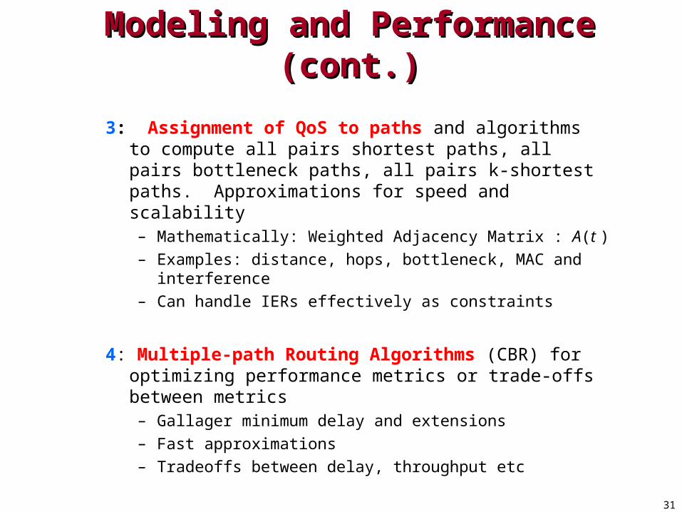
3: Assignment of QoS to paths and algorithms to compute all pairs shortest paths, all pairs bottleneck paths, all pairs k-shortest paths. Approximations for speed and scalability– Mathematically: Weighted Adjacency Matrix : A(t )
– Examples: distance, hops, bottleneck, MAC and interference
– Can handle IERs effectively as constraints
4: Multiple-path Routing Algorithms (CBR) for optimizing performance metrics or trade-offs between metrics– Gallager minimum delay and extensions
– Fast approximations
– Tradeoffs between delay, throughput etc
32
Modeling and Performance (cont.)Modeling and Performance (cont.)
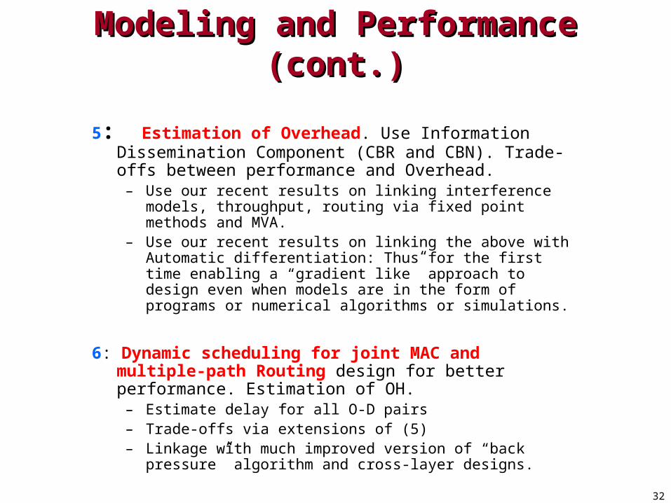
5: Estimation of Overhead. Use Information Dissemination Component (CBR and CBN). Trade-offs between performance and Overhead.
– Use our recent results on linking interference models, throughput, routing via fixed point methods and MVA.
– Use our recent results on linking the above with Automatic differentiation: Thus for the first time enabling a “gradient like” approach to design even when models are in the form of programs or numerical algorithms or simulations.
6: Dynamic scheduling for joint MAC and multiple-path Routing design for better performance. Estimation of OH.
– Estimate delay for all O-D pairs– Trade-offs via extensions of (5)– Linkage with much improved version of “back pressure”
algorithm and cross-layer designs.
5/30/2007 33
Modularity of Routing ProtocolsModularity of Routing Protocols
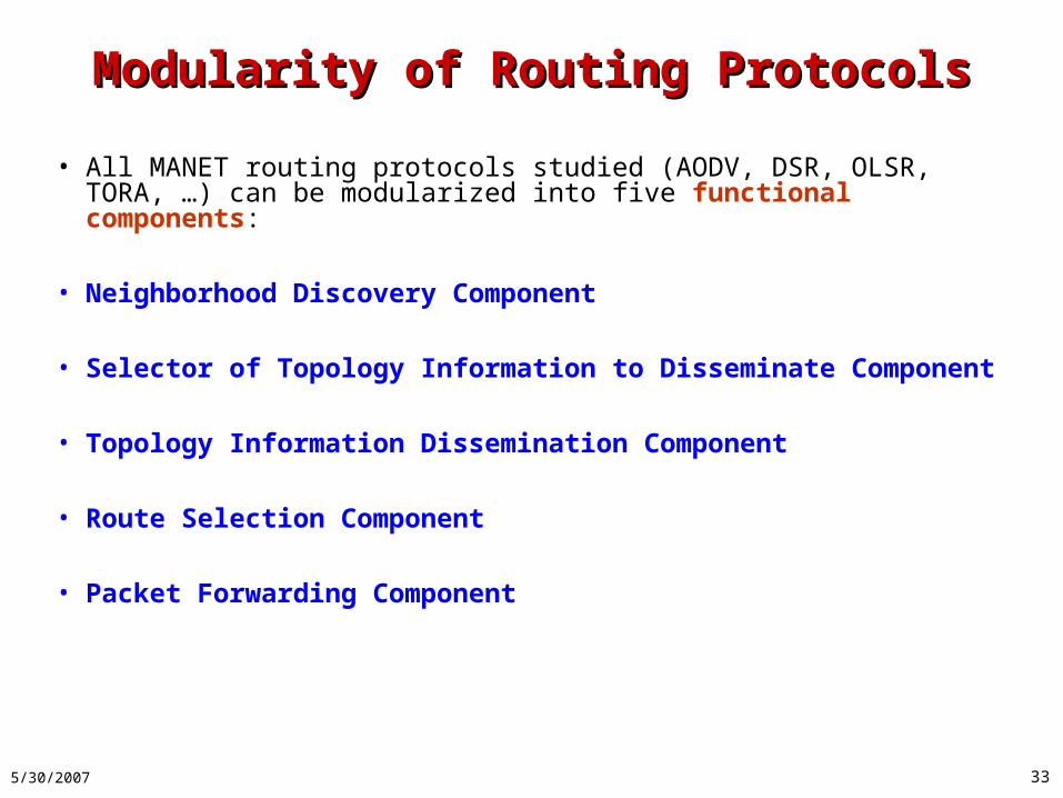
• All MANET routing protocols studied (AODV, DSR, OLSR, TORA, …) can be modularized into five functional components:
• Neighborhood Discovery Component
• Selector of Topology Information to Disseminate Component
• Topology Information Dissemination Component
• Route Selection Component
• Packet Forwarding Component
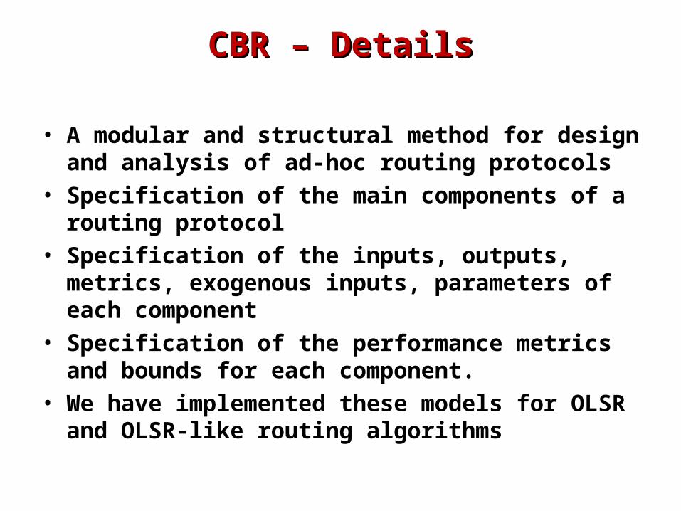
CBR – DetailsCBR – Details
• A modular and structural method for design and analysis of ad-hoc routing protocols
• Specification of the main components of a routing protocol
• Specification of the inputs, outputs, metrics, exogenous inputs, parameters of each component
• Specification of the performance metrics and bounds for each component.
• We have implemented these models for OLSR and OLSR-like routing algorithms
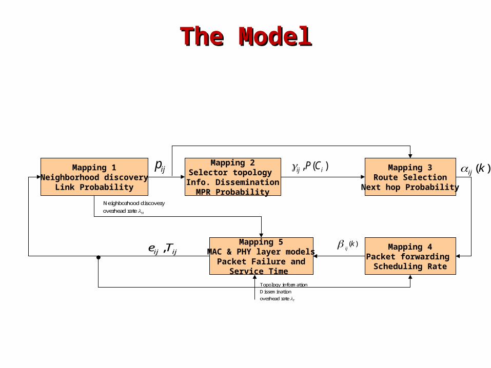
The ModelThe Model
,ij ije T
Mapping 1Neighborhood discovery
Link Probability
Mapping 2Selector topology Info. Dissemination
MPR Probability
Mapping 3Route Selection
Next hop Probability
Mapping 4Packet forwarding
Scheduling Rate
Mapping 5MAC & PHY layer models
Packet Failure andService Time
ijp ( )ij k
( )ijk
, ( )ij iP C
Neighborhood discovery
overhead rate H
Topology information
Dissemination
overhead rate T
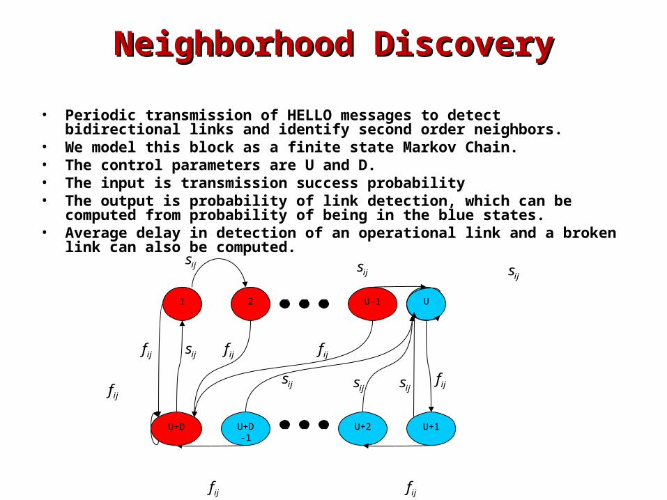
Neighborhood DiscoveryNeighborhood Discovery
• Periodic transmission of HELLO messages to detect bidirectional links and identify second order neighbors.
• We model this block as a finite state Markov Chain.• The control parameters are U and D.• The input is transmission success probability• The output is probability of link detection, which can be computed from
probability of being in the blue states.• Average delay in detection of an operational link and a broken link can also be
computed.
1 2 U
U+2 U+1U+D-1
U-1
U+D
ijfijf
ijf ijf ijf
ijf
ijsijs ijs
ijs ijs ijsijf
ijs
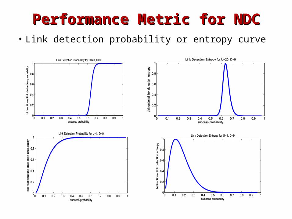
Performance Metric for NDCPerformance Metric for NDC• Link detection probability or entropy curve
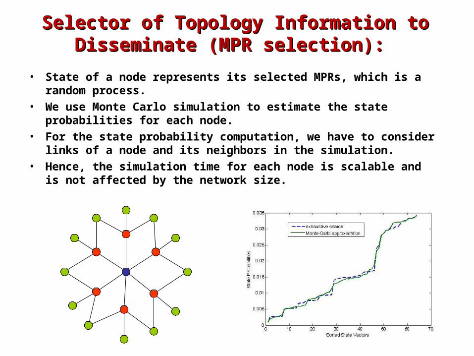
Selector of Topology Information to Disseminate Selector of Topology Information to Disseminate (MPR selection): (MPR selection):
• State of a node represents its selected MPRs, which is a random process.
• We use Monte Carlo simulation to estimate the state probabilities for each node.
• For the state probability computation, we have to consider links of a node and its neighbors in the simulation.
• Hence, the simulation time for each node is scalable and is not affected by the network size.
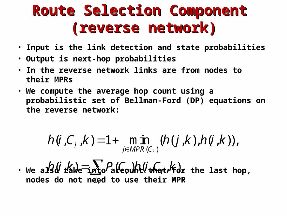
Route Selection Component Route Selection Component (reverse network)(reverse network)
• Input is the link detection and state probabilities• Output is next-hop probabilities• In the reverse network links are from nodes to their MPRs• We compute the average hop count using a probabilistic
set of Bellman-Ford (DP) equations on the reverse network:
• We also take into account that for the last hop, nodes do not need to use their MPR
( )( , , ) 1 min ( ( , ), ( , )),
( , ) ( ) ( , , ).i
i
ij MPR C
i iC
h i C k h j k h i k
h i k P C h i C k
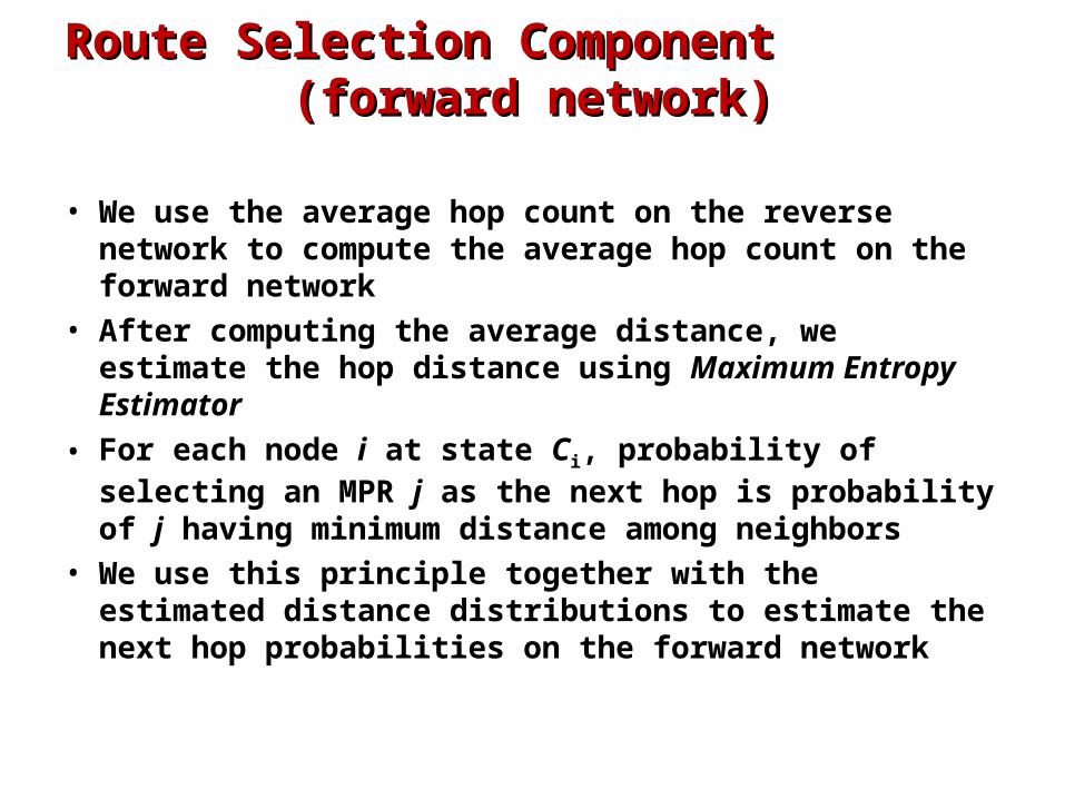
Route Selection Component Route Selection Component (forward network)(forward network)
• We use the average hop count on the reverse network to compute the average hop count on the forward network
• After computing the average distance, we estimate the hop distance using Maximum Entropy Estimator
• For each node i at state Ci, probability of selecting an MPR j as the next hop is probability of j having minimum distance among neighbors
• We use this principle together with the estimated distance distributions to estimate the next hop probabilities on the forward network
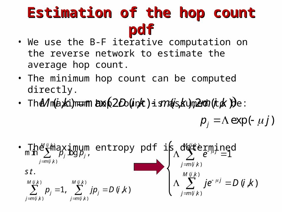
Estimation of the hop count pdfEstimation of the hop count pdf• We use the B-F iterative computation on the reverse
network to estimate the average hop count.• The minimum hop count can be computed directly.• The maximum hop count is assumed to be:
• The maximum entropy pdf is determined
( , ) max 2 ( , ) ( , ),2 ( , )M i k D i k m i k m i k
( , )
( , )
( , ) ( , )
( , ) ( , )
min log ,
. .
1, ( , )
M i k
j jj m i k
M i k M i k
j jj m i k j m i k
p p
s t
p jp D i k
( , )
( , )
( , )
( , )
1
( , )
M i kj
j m i k
M i kj
j m i k
e
je D i k
exp( )jp j
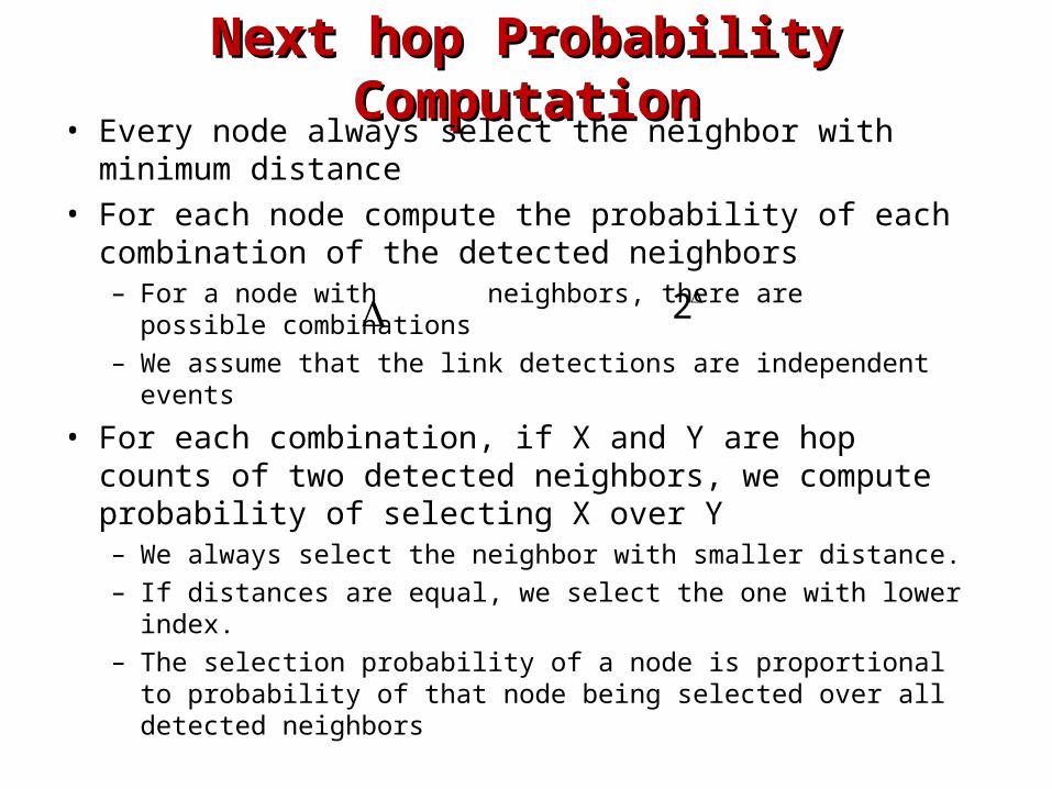
Next hop Probability ComputationNext hop Probability Computation• Every node always select the neighbor with minimum
distance• For each node compute the probability of each
combination of the detected neighbors– For a node with neighbors, there are possible
combinations– We assume that the link detections are independent events
• For each combination, if X and Y are hop counts of two detected neighbors, we compute probability of selecting X over Y– We always select the neighbor with smaller distance.– If distances are equal, we select the one with lower index.– The selection probability of a node is proportional to probability
of that node being selected over all detected neighbors
2
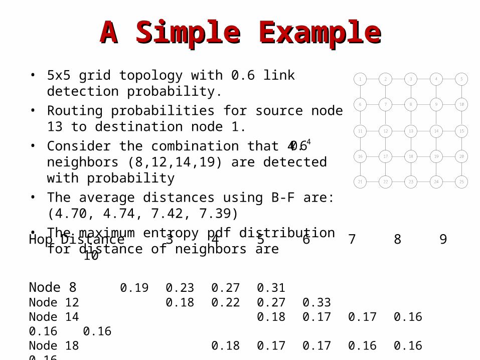
A Simple ExampleA Simple Example• 5x5 grid topology with 0.6 link detection probability.• Routing probabilities for source node 13 to
destination node 1.• Consider the combination that 4 neighbors
(8,12,14,19) are detected with probability• The average distances using B-F are: (4.70, 4.74,
7.42, 7.39) • The maximum entropy pdf distribution for distance
of neighbors are
1 2 3 4 5
6 7 8 9 10
11 12 13 14 15
16 17 18 19 20
21 22 23 24 25
40.6
Hop Distance 3 4 5 6 7 8 9 10
Node 8 0.19 0.23 0.27 0.31Node 12 0.18 0.22 0.27 0.33Node 14 0.18 0.17 0.17 0.16 0.16 0.16Node 18 0.18 0.17 0.17 0.16 0.16 0.16
A Simple Example (cont)A Simple Example (cont)
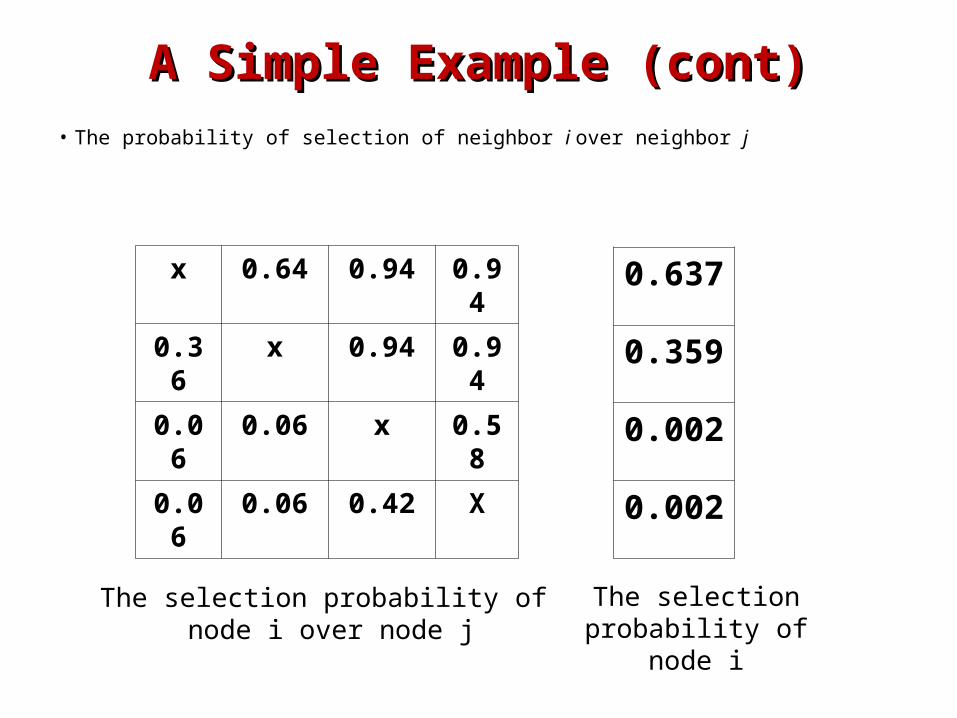
• The probability of selection of neighbor i over neighbor j
x 0.64 0.94 0.94
0.36 x 0.94 0.94
0.06 0.06 x 0.58
0.06 0.06 0.42 X
0.637
0.359
0.002
0.002
The selection probability of node i over node j
The selection probability of node i
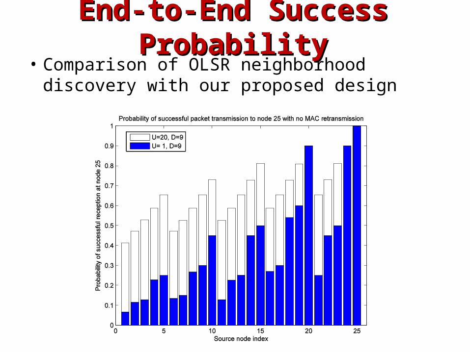
End-to-End Success ProbabilityEnd-to-End Success Probability• Comparison of OLSR neighborhood discovery
with our proposed design
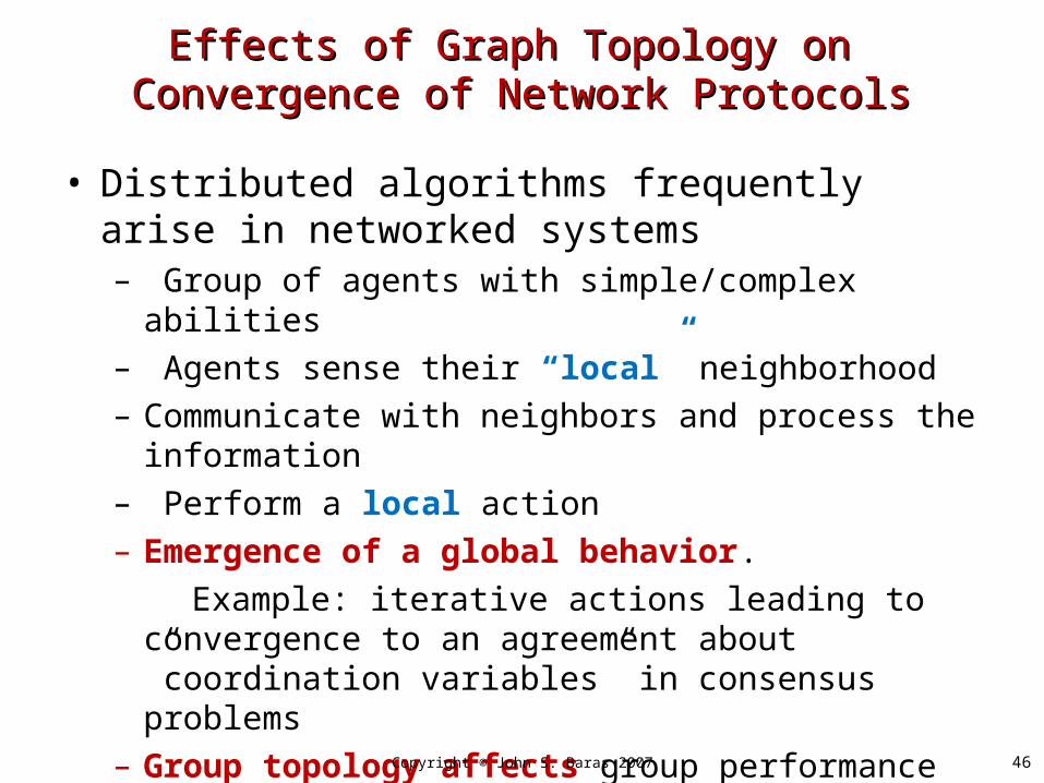
• Distributed algorithms frequently arise in networked systems – Group of agents with simple/complex abilities – Agents sense their “local” neighborhood– Communicate with neighbors and process the
information– Perform a local action– Emergence of a global behavior.
Example: iterative actions leading to convergence to an agreement about ”coordination variables” in consensus problems
– Group topology affects group performance46
Effects of Graph Topology on Effects of Graph Topology on Convergence of Network ProtocolsConvergence of Network Protocols
Copyright © John S. Baras 2007
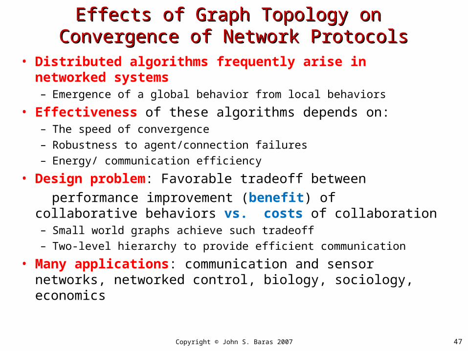
• Distributed algorithms frequently arise in networked systems – Emergence of a global behavior from local behaviors
• Effectiveness of these algorithms depends on:– The speed of convergence– Robustness to agent/connection failures– Energy/ communication efficiency
• Design problem: Favorable tradeoff between
performance improvement (benefit) of collaborative behaviors vs. costs of collaboration– Small world graphs achieve such tradeoff– Two-level hierarchy to provide efficient communication
• Many applications: communication and sensor networks, networked control, biology, sociology, economics
47Copyright © John S. Baras 2007
Effects of Graph Topology on Effects of Graph Topology on Convergence of Network ProtocolsConvergence of Network Protocols

The Importance of Being The Importance of Being Well-ConnectedWell-Connected
• Local majority voting (Peleg ’96)– Each of n citizens has an opinion about voting
Yes or No– Rule: Each citizen’s vote is based on the
majority of its neighbors, including itself– What is the minimum number of No-voters
that can guarantee a No result?– A few number of well connected nodes can
determine the outcome of the process!
48Copyright © John S. Baras 2007
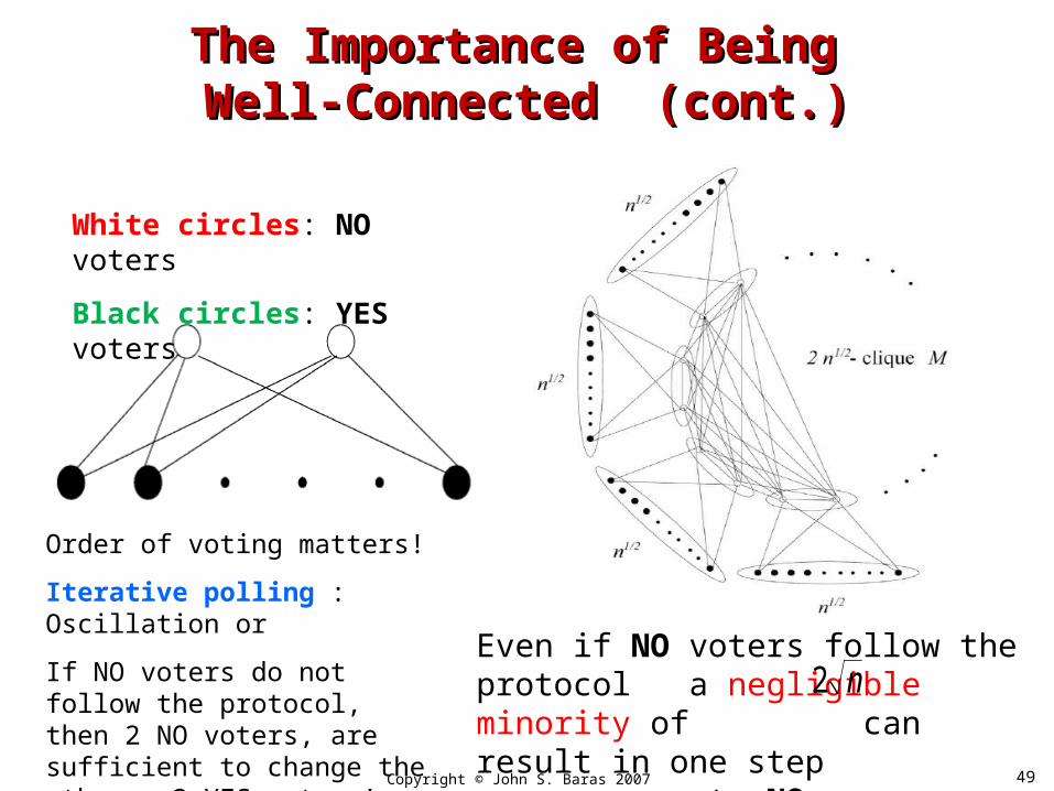
Order of voting matters!
Iterative polling : Oscillation or
If NO voters do not follow the protocol, then 2 NO voters, are sufficient to change the other n-2 YES voters’ opinion.
White circles: NO voters
Black circles: YES voters
Even if NO voters follow the protocol a negligible minority of can result in one step convergence to NO
n2
49Copyright © John S. Baras 2007
The Importance of Being The Importance of Being Well-Connected (cont.)Well-Connected (cont.)
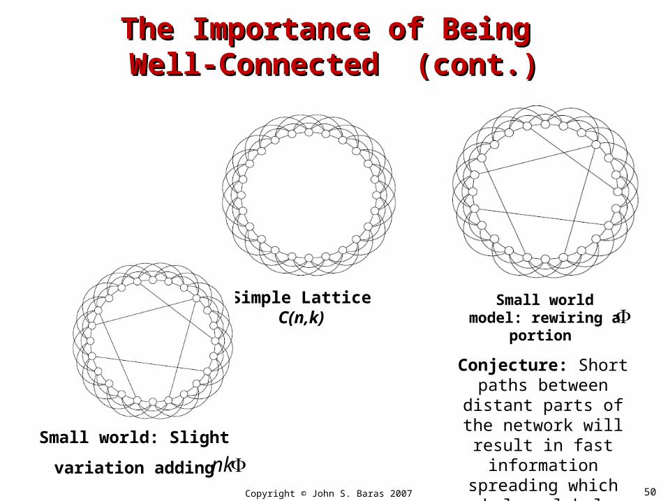
Simple Lattice C(n,k)
Small world model: rewiring a portion
Small world: Slight
variation adding
Conjecture: Short paths between distant parts of the network will result in
fast information spreading which helps global
coordination
nk50
The Importance of Being The Importance of Being Well-Connected (cont.)Well-Connected (cont.)
Copyright © John S. Baras 2007
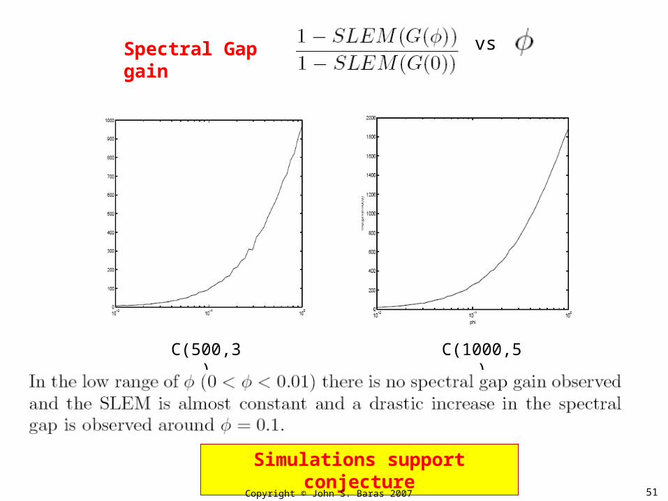
C(500,3) C(1000,5)
Spectral Gap gain vs
Simulations support conjecture
51Copyright © John S. Baras 2007
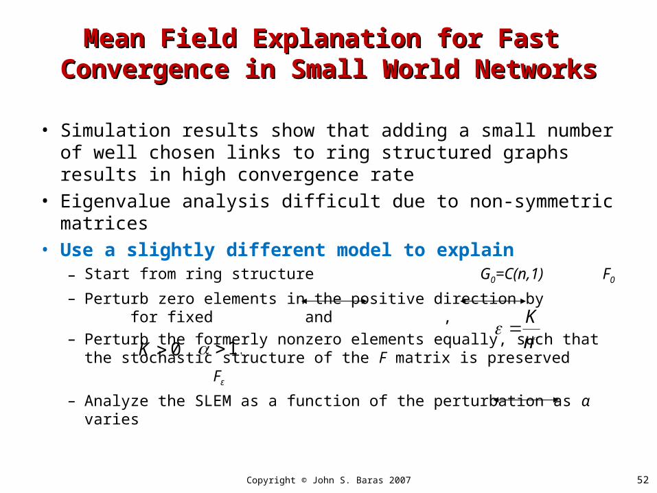
Mean Field Explanation for Fast Mean Field Explanation for Fast Convergence in Small World NetworksConvergence in Small World Networks
• Simulation results show that adding a small number of well chosen links to ring structured graphs results in high convergence rate
• Eigenvalue analysis difficult due to non-symmetric matrices
• Use a slightly different model to explain– Start from ring structure G0=C(n,1) F0
– Perturb zero elements in the positive direction by for fixed and ,
– Perturb the formerly nonzero elements equally, such that the stochastic structure of the F matrix is preserved Fε
– Analyze the SLEM as a function of the perturbation as α varies
n
K0K .1
52Copyright © John S. Baras 2007
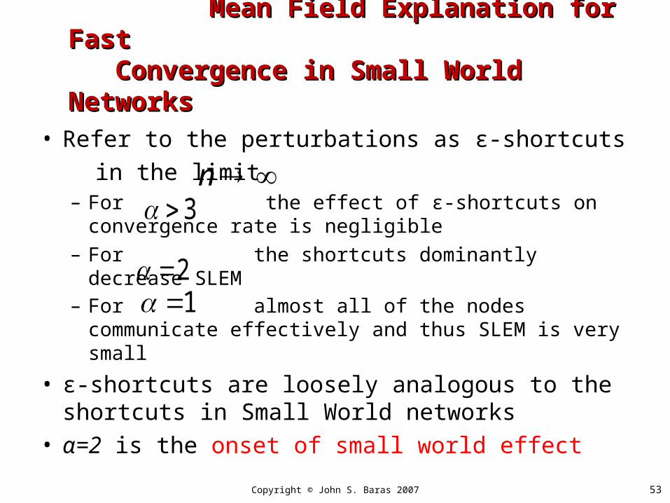
• Refer to the perturbations as ε-shortcuts
in the limit– For the effect of ε-shortcuts on convergence
rate is negligible– For the shortcuts dominantly decrease SLEM– For almost all of the nodes communicate
effectively and thus SLEM is very small
• ε-shortcuts are loosely analogous to the shortcuts in Small World networks
• α=2 is the onset of small world effect
n3
21
53
Mean Field Explanation for Fast Mean Field Explanation for Fast Convergence in Small World Networks Convergence in Small World Networks
Copyright © John S. Baras 2007

54Copyright © John S. Baras 2008
Thank you!
301- 405- 6606
http://www.isr.umd.edu/~baras
Questions?


![Student’s t Sensitivities: GreeksfortheGossetFormulaearXiv:1003.1344v2 [q-fin.PR] 16 Jul 2010 Student’st-DistributionBasedOption Sensitivities: GreeksfortheGossetFormulae Daniel](https://img.pdfslide.net/doc/110x75/5fa1f5e65b7bfb78540e321a/studentas-t-sensitivities-greeksforthegossetformulae-arxiv10031344v2-q-finpr.jpg)