Embed Size (px)
Citation preview
Wireless Physical Layer Security: TowardsPractical Assumptions and Requirements
Biao He
June 2016
A Thesis Submitted for the Degree of
Doctor of Philosophy
of The Australian National University
Research School of Engineering
College of Engineering and Computer Science
The Australian National University
c© Copyright by Biao He 2016


Declaration
The contents of this thesis are the results of original research and have not been submitted for
a higher degree to any other university or institution.
Much of the work in this thesis has been published or has been submitted for publication as
journal papers or conference proceedings.
The research work presented in this thesis has been performed jointly with Dr. Xiangyun Zhou
(The Australian National University), Dr. Nan Yang (The Australian National University),
Prof. Thushara D. Abhayapala (The Australian National University), Prof. Jinhong Yuan (The
University of New South Wales), and Prof. A. Lee Swindlehurst (University of California,
Irvine). The substantial majority of this work was my own.
Biao He
Research School of Engineering,
College of Engineering and Computer Science,
The Australian National University,
Canberra, ACT 2601,
Australia.
iii


Acknowledgments
I would like to express my sincere gratitude to my principal supervisor Dr. Xiangyun Zhou
for his guidance, support, and encouragement throughout my entire PhD journey. I could not
imagine having a better advisor and mentor for my PhD study. I would also like to thank the
chair of my supervision panel Dr. Salman Durrani for his valuable advice on my thesis.
My sincere thanks go to Dr. Nan Yang (The Australian National University), Prof. Thushara
D. Abhayapala (The Australian National University), and Prof. A. Lee Swindlehurst (Univer-
sity of California, Irvine) for their constructive guidance and suggestion on some of the work
produced during my PhD study. I would also like to thank Prof. Parastoo Sadeghi (The Aus-
tralian National University) and Prof. Mark C. Reed (The University of New South Wales,
Canberra) for their valuable career advice.
I would like to thank Prof. Jinhong Yuan from The University of New South Wales, Prof.
Zhu Han from University of Houston, Prof. Lingyang Song from Peking University, and Prof.
Zesong Fei from Beijing Institute of Technology for kindly welcoming me to visit their groups.
The valuable discussion with Prof. Yuan led to part of the work presented in this thesis and the
precious discussion with Prof. Han stimulated many interesting ideas in my work.
Thanks must go to The Australian National University for providing the PhD scholarship
and a great environment supporting my research. It is my great pleasure to study in the Applied
Signal Processing (ASP) group at the Research School of Engineering. I would like to thank
all my friends at the ASP group who made my study here fun and enjoyable.
I would like to give my most sincere thanks to my parents for their continuous support in
general. Last but not the least, I would like to give my special thanks to my partner Yimeng
Jiang for her company, encouragement, and understanding.
v

Abstract
The current research on physical layer security is far from implementations in practical net-
works, arguably due to impractical assumptions in the literature and the limited applicability
of physical layer security. Aiming to reduce the gap between theory and practice, this thesis
focuses on wireless physical layer security towards practical assumptions and requirements.
In the first half of the thesis, we reduce the dependence of physical layer security on imprac-
tical assumptions. The secrecy enhancements and analysis based on impractical assumptions
cannot lead to any true guarantee of secrecy in practical networks. The current study of phys-
ical layer security was often based on the idealized assumption of perfect channel knowledge
on both legitimate users and eavesdroppers. We study the impact of channel estimation errors
on secure transmission designs. We investigate the practical scenarios where both the trans-
mitter and the receiver have imperfect channel state information (CSI). Our results show how
the optimal transmission design and the achievable throughput vary with the amount of knowl-
edge on the eavesdropper’s channel. Apart from the assumption of perfect CSI, the analysis
of physical layer security often ideally assumed the number of eavesdropper antennas to be
known. We develop an innovative approach to study secure communication systems without
knowing the number of eavesdropper antennas by introducing the concept of spatial constraint
into physical layer security. That is, the eavesdropper is assumed to have a limited spatial re-
gion to place (possibly an infinite number of) antennas. We show that a non-zero secrecy rate
is achievable with the help of a friendly jammer, even if the eavesdropper places an infinite
number of antennas in its spatial region.
In the second half of the thesis, we improve the applicability of physical layer security. The
current physical layer security techniques to achieve confidential broadcasting were limited to
application in single-cell systems. The primary challenge to achieve confidential broadcasting
in the multi-cell network is to deal with not only the inter-cell but also the intra-cell information
leakage and interference. To tackle this challenge, we design linear precoders performing con-
fidential broadcasting in multi-cell networks. We optimize the precoder designs to maximize
the secrecy sum rate with based on the large-system analysis. Finally, we improve the appli-
cability of physical layer security from a fundamental aspect. The analysis of physical layer
security based on the existing secrecy metric was often not applicable in practical networks.
We propose new metrics for evaluating the secrecy of transmissions over fading channels to ad-
dress the practical limitations of using existing secrecy metrics for such evaluations. The first
metric establishes a link between the concept of secrecy outage and the eavesdropper’s ability
to decode confidential messages. The second metric provides an error-probability-based se-
vii

viii
crecy metric which is often used for the practical implementation of secure wireless systems.
The third metric characterizes how much or how fast the confidential information is leaked
to the eavesdropper. We show that the proposed secrecy metrics enable one to appropriately
design secure communication systems with different views on how secrecy is measured.
List of Publications
Journal Articles
J1. B. He and X. Zhou, “Secure on-off transmission design with channel estimation errors,"
IEEE Trans. Inf. Forensics Security, vol. 8, no. 12, pp. 1923–1936, Dec. 2013.
J2. B. He, N. Yang, X. Zhou, and J. Yuan, “Base station cooperation for confidential broad-
casting in multi-cell networks," IEEE Trans. Wireless Commun., vol. 14, no. 10, pp.
5287–5299, Oct. 2015.
J3. B. He, X. Zhou, and T. D. Abhayapala, “Achieving secrecy without knowing the number
of eavesdropper antennas," IEEE Trans. Wireless Commun., vol. 14, no. 12, pp. 7030–
7043, Dec. 2015.
J4. B. He, X. Zhou, and A. L. Swindlehurst, “On secrecy metrics for physical layer security
over quasi-static fading channels," submitted to IEEE Trans. Wireless Commun., Jan.
2016.
J5. B. He, X. Zhou, and T. D. Abhayapala, “Wireless physical layer security with imperfect
channel state information: A survey,” ZTE Communications, vol. 11, no. 3, pp. 11–19,
Sept. 2013. (invited paper)
J6. X. Xu, B. He, W. Yang, X. Zhou, and Y. Cai, “Secure transmission design for cognitive
radio networks with Poisson distributed eavesdroppers,” IEEE Trans. Inf. Forensics
Security, vol. 11, no. 2, pp. 373–387, Feb. 2016. (not included in the thesis)
Conference Papers
C1. B. He and X. Zhou, “Impact of channel estimation error on secure transmission design,”
in Proc. IEEE AusCTW, Adelaide, SA, Jan. 2013, pp. 19–24.
C2. B. He and X. Zhou, “New physical layer security measures for wireless transmissions
over fading channels,” in Proc. IEEE GLOBECOM, Austin, TX, Dec. 2014, pp. 722–
727.
C3. B. He, N. Yang, X. Zhou, and J. Yuan, “Confidential broadcasting via coordinated beam-
forming in two-cell networks,” in Proc. IEEE ICC, London, UK, June 2015, pp. 7376–
7382.
ix

x
C4. B. He and X. Zhou, “On the placement of RF energy harvesting node in wireless networks
with secrecy considerations,” in Proc. IEEE GLOBECOM Workshop, Austin, TX, Dec.
2014, pp. 1355–1360. (not included in the thesis)
C5. Y. Cai, X. Xu, B. He, W. Yang, and X. Zhou, “Protecting cognitive radio networks against
Poisson distributed eavesdroppers,” in Proc. IEEE ICC, Kuala Lumpur, Malaysia, May
2016, pp. 4035–4041. (not included in the thesis)

Acronyms
AN artificial noise
AWGN additive white Gaussian noise
BD block diagonalization
BS base station
CBf coordinated beamforming
CSI channel state information
dB decibel
i.i.d. independent and identically distributed
MCP multi-cell processing
MIMO multi-input multi-output
MISO multi-input single-output
MMSE minimum mean square error
MRT maximum ratio transmission
RCI regularized channel inversion
RZF regularized zero forcing
SINR signal-to-interference-plus-noise ratio
SNR signal-to-noise ratio
UCA uniform circular array
ULA uniform linear array
2D two-dimensional
3D three-dimensional
xi


Notations
| · | magnitude of an element
|X| determinant of matrix X
‖ · ‖ Euclidean norm of a vector
In identity matrix with size n×n
(·)T transpose of a vector or a matrix
(·)H conjugate transpose of a vector or a matrix
logn() logarithm to base n
ln(·) natural logarithm
d·e ceiling operator
b·c floor operator
E{·} expectation operator
P{·} probability measure
Tr(·) trace of a matrix
[x]+ max(x,0)
a.s−→ almost sure convergence
i.p−→ convergence in probability
CN(µ ,σ2
)circularly symmetric complex Gaussian distribution with mean µ and variance σ2
max{·} maximization
min{·} minimization
W0 {·} the principal branch of the Lambert W function
xiii

Contents
Declaration iii
Acknowledgments v
Abstract vii
List of Publications ix
Acronyms xi
Notations xiii
1 Introduction 11.1 Fundamentals and Background . . . . . . . . . . . . . . . . . . . . . . . . . . 2
1.1.1 Information-Theoretic Secrecy and Wiretap Channel . . . . . . . . . . 2
1.1.2 Secrecy Metrics for Wireless Transmissions . . . . . . . . . . . . . . . 4
1.1.2.1 Ergodic Secrecy Capacity . . . . . . . . . . . . . . . . . . . 4
1.1.2.2 Secrecy Outage Probability . . . . . . . . . . . . . . . . . . 5
1.1.3 Signal Processing Secrecy Enhancements . . . . . . . . . . . . . . . . 6
1.1.3.1 Secure On-Off Transmission Scheme . . . . . . . . . . . . . 6
1.1.3.2 Beamforming with AN . . . . . . . . . . . . . . . . . . . . 7
1.1.3.3 Linear Precoding for Confidential Broadcasting . . . . . . . 9
1.2 Motivation and Challenges . . . . . . . . . . . . . . . . . . . . . . . . . . . . 10
1.2.1 Impractical Assumptions . . . . . . . . . . . . . . . . . . . . . . . . . 10
1.2.2 Limited Applicability . . . . . . . . . . . . . . . . . . . . . . . . . . . 11
1.3 Thesis Outline and Contributions . . . . . . . . . . . . . . . . . . . . . . . . . 12
2 Secure On-Off Transmission Design with Channel Estimation Errors 192.1 Introduction . . . . . . . . . . . . . . . . . . . . . . . . . . . . . . . . . . . . 19
2.2 System Model . . . . . . . . . . . . . . . . . . . . . . . . . . . . . . . . . . . 20
2.2.1 Channel Estimation . . . . . . . . . . . . . . . . . . . . . . . . . . . . 22
2.2.2 Channel Knowledge . . . . . . . . . . . . . . . . . . . . . . . . . . . 23
2.2.3 Secure Encoding . . . . . . . . . . . . . . . . . . . . . . . . . . . . . 24
2.3 On-Off Transmission Design . . . . . . . . . . . . . . . . . . . . . . . . . . . 25
xv
xvi Contents
2.3.1 Scenario One . . . . . . . . . . . . . . . . . . . . . . . . . . . . . . . 26
2.3.2 Scenario Two . . . . . . . . . . . . . . . . . . . . . . . . . . . . . . . 29
2.3.3 Scenario Three . . . . . . . . . . . . . . . . . . . . . . . . . . . . . . 31
2.4 Joint Rate and On-Off Transmission Design . . . . . . . . . . . . . . . . . . . 32
2.4.1 Non-Adaptive Rate Scheme . . . . . . . . . . . . . . . . . . . . . . . 33
2.4.2 Adaptive Rate Scheme . . . . . . . . . . . . . . . . . . . . . . . . . . 35
2.5 Numerical Results . . . . . . . . . . . . . . . . . . . . . . . . . . . . . . . . . 37
2.5.1 On-Off Transmission Design . . . . . . . . . . . . . . . . . . . . . . . 37
2.5.2 Joint Rate and On-Off Transmission Design . . . . . . . . . . . . . . . 40
2.6 Summary . . . . . . . . . . . . . . . . . . . . . . . . . . . . . . . . . . . . . 42
3 Achieving Secrecy without Knowing the Number of Eavesdropper Antennas 453.1 Introduction . . . . . . . . . . . . . . . . . . . . . . . . . . . . . . . . . . . . 45
3.2 System Model . . . . . . . . . . . . . . . . . . . . . . . . . . . . . . . . . . . 46
3.2.1 Wiretap-Channel System . . . . . . . . . . . . . . . . . . . . . . . . . 47
3.2.2 Jammer-Assisted System . . . . . . . . . . . . . . . . . . . . . . . . . 49
3.2.2.1 Case 1: Basic Jammer-Assisted System . . . . . . . . . . . . 49
3.2.2.2 Case 2: AN Jammer-Assisted System . . . . . . . . . . . . . 50
3.3 Introducing Spatial Constraints into Secrecy Capacity Calculation . . . . . . . 51
3.3.1 Secrecy Capacity of Wiretap-Channel System . . . . . . . . . . . . . . 52
3.3.2 Secrecy Capacity of Basic Jammer-Assisted System . . . . . . . . . . 53
3.3.3 Secrecy Capacity of AN Jammer-Assisted System . . . . . . . . . . . 53
3.3.4 Secrecy Capacity with Legitimate CSI Available at Alice . . . . . . . . 54
3.3.5 Numerical Results . . . . . . . . . . . . . . . . . . . . . . . . . . . . 55
3.4 Worst-Case Analysis for Jammer-Assisted Systems . . . . . . . . . . . . . . . 58
3.4.1 Wiretap-Channel System . . . . . . . . . . . . . . . . . . . . . . . . . 58
3.4.2 Basic Jammer-Assisted System . . . . . . . . . . . . . . . . . . . . . 59
3.4.2.1 Worst-Case Secrecy Capacity . . . . . . . . . . . . . . . . . 59
3.4.2.2 Optimal Jamming Power . . . . . . . . . . . . . . . . . . . 60
3.4.3 AN Jammer-Assisted System . . . . . . . . . . . . . . . . . . . . . . 61
3.4.4 Numerical Results . . . . . . . . . . . . . . . . . . . . . . . . . . . . 62
3.5 Summary . . . . . . . . . . . . . . . . . . . . . . . . . . . . . . . . . . . . . 66
4 Base Station Cooperation for Confidential Broadcasting in Multi-Cell Networks 674.1 Introduction . . . . . . . . . . . . . . . . . . . . . . . . . . . . . . . . . . . . 67
4.2 Network Model . . . . . . . . . . . . . . . . . . . . . . . . . . . . . . . . . . 68
4.2.1 Confidential Broadcasting and Performance Metric . . . . . . . . . . . 70
4.2.2 Multi-Cell Processing with RCI Precoder . . . . . . . . . . . . . . . . 71
Contents xvii
4.2.3 Coordinated Beamforming with Generalized RCI Precoder . . . . . . . 73
4.3 Secrecy Sum Rate in the Large-System Regime . . . . . . . . . . . . . . . . . 75
4.3.1 Large-System Analysis . . . . . . . . . . . . . . . . . . . . . . . . . . 75
4.3.2 Numerical Results . . . . . . . . . . . . . . . . . . . . . . . . . . . . 76
4.4 Optimization of Secrecy Sum Rate . . . . . . . . . . . . . . . . . . . . . . . . 78
4.4.1 Optimal Regularization Parameter . . . . . . . . . . . . . . . . . . . . 78
4.4.1.1 α∗MCP for MCP . . . . . . . . . . . . . . . . . . . . . . . . . 79
4.4.1.2 α∗CBf for CBf . . . . . . . . . . . . . . . . . . . . . . . . . . 79
4.4.1.3 Numerical Results . . . . . . . . . . . . . . . . . . . . . . . 79
4.4.2 Power-Reduction Strategy . . . . . . . . . . . . . . . . . . . . . . . . 84
4.4.2.1 Power Reduction for MCP . . . . . . . . . . . . . . . . . . 85
4.4.2.2 Power Reduction for CBf . . . . . . . . . . . . . . . . . . . 85
4.4.2.3 Numerical Results . . . . . . . . . . . . . . . . . . . . . . . 86
4.5 Summary . . . . . . . . . . . . . . . . . . . . . . . . . . . . . . . . . . . . . 87
5 New Secrecy Metrics for Wireless Transmission over Fading Channels 895.1 Introduction . . . . . . . . . . . . . . . . . . . . . . . . . . . . . . . . . . . . 89
5.2 Perfect Secrecy and Partial Secrecy . . . . . . . . . . . . . . . . . . . . . . . . 90
5.2.1 Perfect Secrecy . . . . . . . . . . . . . . . . . . . . . . . . . . . . . . 90
5.2.2 Partial Secrecy . . . . . . . . . . . . . . . . . . . . . . . . . . . . . . 91
5.3 New Secrecy Metrics for Wireless Transmissions . . . . . . . . . . . . . . . . 92
5.3.1 Fractional Equivocation for a Given Fading Realization . . . . . . . . . 92
5.3.2 New Secrecy Metrics . . . . . . . . . . . . . . . . . . . . . . . . . . . 93
5.3.2.1 Generalized Secrecy Outage Probability . . . . . . . . . . . 93
5.3.2.2 Average Fractional Equivocation . . . . . . . . . . . . . . . 93
5.3.2.3 Average Information Leakage Rate . . . . . . . . . . . . . . 94
5.4 Wireless Transmissions with Non-Adaptive Rate Wiretap Codes: An Example . 94
5.4.1 System Model . . . . . . . . . . . . . . . . . . . . . . . . . . . . . . 94
5.4.2 Secrecy Performance Evaluation . . . . . . . . . . . . . . . . . . . . . 95
5.4.2.1 Generalized Secrecy Outage Probability . . . . . . . . . . . 96
5.4.2.2 Average Fractional Equivocation . . . . . . . . . . . . . . . 97
5.4.2.3 Average Information Leakage Rate . . . . . . . . . . . . . . 97
5.4.3 Numerical Results . . . . . . . . . . . . . . . . . . . . . . . . . . . . 97
5.5 Impact on System Designs . . . . . . . . . . . . . . . . . . . . . . . . . . . . 100
5.5.1 Problem Formulation . . . . . . . . . . . . . . . . . . . . . . . . . . . 101
5.5.2 Feasibility of the Constraint . . . . . . . . . . . . . . . . . . . . . . . 102
5.5.3 Optimal Rate Parameters . . . . . . . . . . . . . . . . . . . . . . . . . 102
5.5.4 Numerical Results . . . . . . . . . . . . . . . . . . . . . . . . . . . . 103

xviii Contents
5.6 Summary . . . . . . . . . . . . . . . . . . . . . . . . . . . . . . . . . . . . . 106
6 Conclusions 1096.1 Thesis Conclusions . . . . . . . . . . . . . . . . . . . . . . . . . . . . . . . . 109
6.2 Future Research Directions . . . . . . . . . . . . . . . . . . . . . . . . . . . . 110
A Appendix A 111A.1 Proof of Proposition 2.1 . . . . . . . . . . . . . . . . . . . . . . . . . . . . . . 111
A.2 Proof of Proposition 2.2 . . . . . . . . . . . . . . . . . . . . . . . . . . . . . . 112
A.3 Proof of Proposition 2.4 . . . . . . . . . . . . . . . . . . . . . . . . . . . . . . 112
A.4 Proof of Proposition 2.5 . . . . . . . . . . . . . . . . . . . . . . . . . . . . . . 113
B Appendix B 115B.1 Proof of Proposition 3.1 . . . . . . . . . . . . . . . . . . . . . . . . . . . . . . 115
B.2 Proof of Theorem 3.1 . . . . . . . . . . . . . . . . . . . . . . . . . . . . . . . 117
B.3 Proof of Theorem 3.2 . . . . . . . . . . . . . . . . . . . . . . . . . . . . . . . 119
B.4 Proof of Proposition 3.2 . . . . . . . . . . . . . . . . . . . . . . . . . . . . . . 120
C Appendix C 123C.1 Proof of Theorem 4.1 . . . . . . . . . . . . . . . . . . . . . . . . . . . . . . . 123
C.2 Proof of Theorem 4.2 . . . . . . . . . . . . . . . . . . . . . . . . . . . . . . . 125
D Appendix D 129D.1 Proof of Proposition 5.2 . . . . . . . . . . . . . . . . . . . . . . . . . . . . . . 129
D.2 Proof of Proposition 5.3 . . . . . . . . . . . . . . . . . . . . . . . . . . . . . . 129
D.3 Proof of Proposition 5.4 . . . . . . . . . . . . . . . . . . . . . . . . . . . . . . 130
Bibliography 133

List of Figures
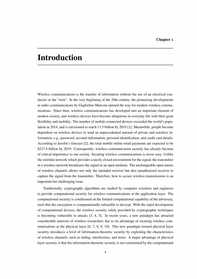
1.1 Illustration of a wireless network with an eavesdropper. . . . . . . . . . . . . . 2
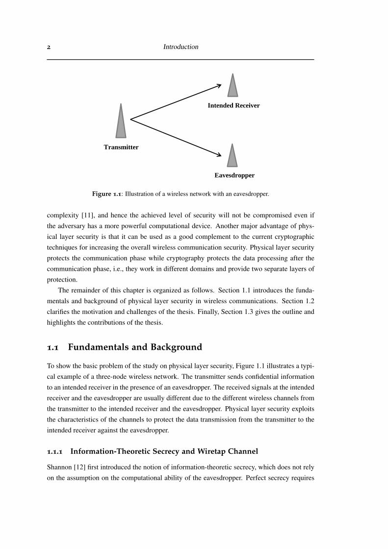
1.2 Wiretap-channel model. . . . . . . . . . . . . . . . . . . . . . . . . . . . . . . 3
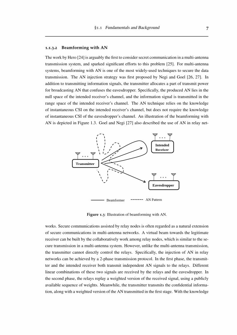
1.3 Illustration of beamforming with AN. . . . . . . . . . . . . . . . . . . . . . . 7
1.4 Illustration of confidential broadcasting in a single-cell network. . . . . . . . . 9
2.1 Scenario 1: Achievable throughput versus normalized pilot power for different
average received data SNRs at Bob, αb = 5 dB, 10 dB, 15 dB, 20 dB. The
other system parameters are δ = 0.1, ϕ = 0.05, αe = 0 dB, Rb = 2, Rs = 1. . . 37
2.2 Scenario 2: Achievable throughput versus normalized pilot power for different
average received data SNRs at Bob, αb = 5 dB, 10 dB, 15 dB, 20 dB. The
other system parameters are δ = 0.1, ϕ = 0.05, αe = 0 dB, Rb = 2, Rs = 1. . . 38
2.3 Achievable throughput versus secrecy constraint for different values of nor-
malized pilot power, ψ = 1, 5, ∞. The other system parameters are αb = 10
dB, αe = 0 dB, δ = 0.1, Rb = 2, Rs = 1. . . . . . . . . . . . . . . . . . . . . . 39
2.4 Non-adaptive rate scheme: feasible secrecy constraint versus feasible reliabil-
ity constraint for different values of normalized pilot power, ψ = 1, 5, ∞. The
other system parameters are µb = 9, αb = 10 dB, αe = 0 dB. . . . . . . . . . . 40
2.5 Achievable throughput versus secrecy constraint for different values of nor-
malized pilot power, ψ = 1, 5. The other system parameters are δ = 0.1,
αb = 10 dB, αe = 0 dB. . . . . . . . . . . . . . . . . . . . . . . . . . . . . . . 41
2.6 Achievable secrecy constraint versus normalized pilot power for different tar-
get throughput values, η = 0.2, 0.5. The other system parameters are δ = 0.1,
αb = 10 dB, αe = 0 dB. . . . . . . . . . . . . . . . . . . . . . . . . . . . . . . 42
3.1 2D model for the wiretap-channel system. . . . . . . . . . . . . . . . . . . . . 47
3.2 3D model for the wiretap-channel system. . . . . . . . . . . . . . . . . . . . . 48
3.3 2D model for the jammer-assisted system. . . . . . . . . . . . . . . . . . . . . 49
3.4 3D model for the jammer-assisted system. . . . . . . . . . . . . . . . . . . . . 50
3.5 Wiretap-channel system: Secrecy capacity versus the number of Bob’s anten-
nas and the number of Eve’s antennas. Bob and Eve are spatially constrained
by circular apertures with radii rb = 1.5λ and re = 1λ , respectively. . . . . . . 55
xix

xx LIST OF FIGURES
3.6 Basic jammer-assisted system: Secrecy capacity versus the number of Bob’s
antennas and the number of Eve’s antennas. Bob and Eve are spatially con-
strained by circular apertures with radii rb = 1.5λ and re = 1λ , respectively. . . 55
3.7 AN jammer-assisted system: Secrecy capacity versus the number of Bob’s
antennas and the number of Eve’s antennas. Bob and Eve are spatially con-
strained by circular apertures with radii rb = 1.5λ and re = 1λ , respectively. . . 56
3.8 Secrecy capacity versus the number of eavesdropper antennas with Nb = 35.
Bob and Eve are spatially constrained by circular apertures with radii rb =
1.5λ and re = 1λ , respectively. . . . . . . . . . . . . . . . . . . . . . . . . . . 57
3.9 The minimum number of Bob’s antennas for achieving a non-zero worst-case
secrecy capacity versus the radius of Eve’s spatial constraint. The other system
parameters are Pt = 20 dB,Pj = 0 dB,αb = 1,αe = 1,βb = 1,βe = 1,σ2b =
1 and rb = 2λ . . . . . . . . . . . . . . . . . . . . . . . . . . . . . . . . . . . . 63
3.10 The worst-case secrecy capacity versus the radius of Eve’s spatial constraint.
The other system parameters are Pt = 20 dB,Pj = 0 dB,αb = 1,αe = 1,βb =
1,βe = 1,σ2b = 1,rb = 2λ and Nb = N0b = 37. . . . . . . . . . . . . . . . . . . 64
3.11 The worst-case secrecy capacity versus the jamming power. The other sys-
tem parameters are Pt = 20 dB,αb = 1,αe = 1,βb = 1,βe = 1,σ2b = 1,rb =
1.5λ ,re = 1λ and Nb = 30. . . . . . . . . . . . . . . . . . . . . . . . . . . . . 65
4.1 Illustration of a symmetric two-cell broadcast network, where each cell con-
sists of one N-antenna BS and K single-antenna users. . . . . . . . . . . . . . . 68
4.2 The normalized rate difference versus the number of antennas at each BS for
ε = 0.5,α = 0.2,β = 0.5 and γ = 10 dB. . . . . . . . . . . . . . . . . . . . . 77
4.3 The normalized rate difference versus the cross-cell interference level for N =
20,α = 0.2,β = 0.5 and γ = 10 dB. . . . . . . . . . . . . . . . . . . . . . . . 78
4.4 The large-system secrecy rate per antenna versus the cross-cell interference
level for different designs of the regularization parameter with N = 20,β = 0.5
and γ = 10 dB. . . . . . . . . . . . . . . . . . . . . . . . . . . . . . . . . . . 81
4.5 MCP: the large-system secrecy rate per antenna versus the average transmit
SNR per BS for different designs of the regularization parameter with β =
0.8,1,1.2, N = 20 and ε = 0.5. . . . . . . . . . . . . . . . . . . . . . . . . . . 82
4.6 CBf: the large-system secrecy rate per antenna versus the average transmit
SNR per BS for different designs of the regularization parameter with β =
0.4,0.5,0.6, N = 20 and ε = 0.5. . . . . . . . . . . . . . . . . . . . . . . . . . 83
4.7 The large-system secrecy rate per antenna versus the average transmit SNR per
BS for different designs of the regularization parameter with N = 20 and ε = 0.5. 84
LIST OF FIGURES xxi
4.8 MCP: the large-system secrecy rate per antenna versus the average transmit
SNR per BS for the transmissions with and without power-reduction strategy.
The other system parameters are β = 1.2,1.5,N = 20 and ε = 0.5. . . . . . . . 86
4.9 CBf: the large-system secrecy rate per antenna versus the average transmit
SNR per BS for the transmissions with and without power-reduction strategy.
The other system parameters are β = 0.6,0.8,N = 20 and ε = 0.5. . . . . . . . 87
5.1 Basic wiretap-channel system. . . . . . . . . . . . . . . . . . . . . . . . . . . 90
5.2 Generalized secrecy outage probability versus confidential information rate.
Results are shown for networks with different requirements on the fractional
equivocation, θ = 1,0.8,0.6. The other parameters are Rb = 4 and γe = 1. . . . 98
5.3 Generalized secrecy outage probability versus average received SNR at Eve.
Results are shown for networks with different requirements on the fractional
equivocation, θ = 1,0.8. The other parameters are Rb = Rs = 4. . . . . . . . . 99
5.4 Average fractional equivocation (asymptotic lower bound on the decoding er-
ror probability at Eve) versus confidential information rate. Results are shown
for networks with different average received SNRs at Eve, γe = 1,2. The other
parameter is Rb = 4. . . . . . . . . . . . . . . . . . . . . . . . . . . . . . . . 100
5.5 Average information leakage rate versus confidential information rate. Results
are shown for networks with different average received SNRs at Eve, γe = 1,2.
The other parameter is Rb = 4. . . . . . . . . . . . . . . . . . . . . . . . . . . 101
5.6 For different secrecy metrics: optimal confidential information rate versus
minimum required throughput. The other parameters are θ = 1, γb = 10 dB
and γe = 10 dB. . . . . . . . . . . . . . . . . . . . . . . . . . . . . . . . . . . 104
5.7 For generalized secrecy outage probability: optimal confidential information
rate versus minimum required throughput. Results are shown for networks
with different requirements on the fractional equivocation, θ = 1,0.8,0.6. The
other parameters are γb = 10 dB and γe = 10 dB. . . . . . . . . . . . . . . . . 105
5.8 Secrecy outage probability versus minimum required throughput. The other
parameters are θ = 1, γb = 10 dB and γe = 10 dB. . . . . . . . . . . . . . . . 106
5.9 Average fractional equivocation (asymptotic lower bound on the decoding er-
ror probability at Eve) versus minimum required throughput. The other param-
eters are θ = 1, γb = 10 dB and γe = 10 dB. . . . . . . . . . . . . . . . . . . . 107
5.10 Average information leakage rate versus minimum required throughput. The
other parameters are θ = 1, γb = 10 dB and γe = 10 dB. . . . . . . . . . . . . 108
B.1 Without jamming signals: Ci versus Ni. The other system parameters are Nt =
100,ri = 1λ ,Pt = 10 dB, αi = 1,σ2i = 1. . . . . . . . . . . . . . . . . . . . . 116

xxii LIST OF FIGURES
B.2 With jamming signals: Ci versus Ni. The other system parameters are Nt =
N j = 100,ri = 1λ ,Pt = 10 dB, Pj = 0 dB αi = 1,βi = 1,σ2i = 1. . . . . . . . . 119
Chapter 1
Introduction
Wireless communications is the transfer of information without the use of an electrical con-
ductor or the “wire". In the very beginning of the 20th century, the pioneering developments
in radio communications by Guglielmo Marconi opened the way for modern wireless commu-
nications. Since then, wireless communications has developed into an important element of
modern society, and wireless devices have become ubiquitous in everyday life with their great
flexibility and mobility. The number of mobile-connected devices exceeded the world’s popu-
lation in 2014, and is envisioned to reach 11.5 billion by 2019 [1]. Meanwhile, people become
dependent on wireless devices to send an unprecedented amount of private and sensitive in-
formation, e.g., password, account information, personal identification, and credit card details.
According to Javelin’s forecast [2], the total mobile online retail payments are expected to be
$217.4 billion by 2019. Consequently, wireless communication security has already become
of critical importance to our society. Securing wireless communications is never easy. Unlike
the wireline network which provides a nicely closed environment for the signal, the transmitter
in a wireless network broadcasts the signal in an open medium. The unchangeable open nature
of wireless channels allows not only the intended receiver but also unauthorized receiver to
capture the signal from the transmitter. Therefore, how to secure wireless transmissions is an
important but challenging issue.
Traditionally, cryptography algorithms are studied by computer scientists and engineers
to provide computational security for wireless communications at the application layer. The
computational security is conditioned on the limited computational capability of the adversary,
such that the encryption is computationally infeasible to decrypt. With the rapid development
of computational devices, the wireless security solely provided by cryptographic techniques
is becoming vulnerable to attacks [3, 4, 5]. In recent years, a new paradigm has attracted
considerable interests of wireless researchers due to its advantage of securing wireless com-
munications at the physical layer [6, 7, 8, 9, 10]. This new paradigm termed physical layer
security introduces a level of information-theoretic security by exploiting the characteristics
of wireless channels, such as fading, interference, and noise. A major advantage of physical
layer security is that the information-theoretic security is not constrained by the computational
1
2 Introduction
Transmitter
Eavesdropper
Intended Receiver
Figure 1.1: Illustration of a wireless network with an eavesdropper.
complexity [11], and hence the achieved level of security will not be compromised even if
the adversary has a more powerful computational device. Another major advantage of phys-
ical layer security is that it can be used as a good complement to the current cryptographic
techniques for increasing the overall wireless communication security. Physical layer security
protects the communication phase while cryptography protects the data processing after the
communication phase, i.e., they work in different domains and provide two separate layers of
protection.
The remainder of this chapter is organized as follows. Section 1.1 introduces the funda-
mentals and background of physical layer security in wireless communications. Section 1.2
clarifies the motivation and challenges of the thesis. Finally, Section 1.3 gives the outline and
highlights the contributions of the thesis.
1.1 Fundamentals and Background
To show the basic problem of the study on physical layer security, Figure 1.1 illustrates a typi-
cal example of a three-node wireless network. The transmitter sends confidential information
to an intended receiver in the presence of an eavesdropper. The received signals at the intended
receiver and the eavesdropper are usually different due to the different wireless channels from
the transmitter to the intended receiver and the eavesdropper. Physical layer security exploits
the characteristics of the channels to protect the data transmission from the transmitter to the
intended receiver against the eavesdropper.
1.1.1 Information-Theoretic Secrecy and Wiretap Channel
Shannon [12] first introduced the notion of information-theoretic secrecy, which does not rely
on the assumption on the computational ability of the eavesdropper. Perfect secrecy requires
§1.1 Fundamentals and Background 3
that the amount of information leakage to the eavesdropper vanishes. It guarantees that the
eavesdropper’s optimal attack is to guess the message at random, and hence the eavesdropper’s
decoding error probability, Pe, asymptotically goes to 1. In the seminal work [13], Wyner
introduced the wiretap-channel system, and addressed the tradeoff between the information
rate to the intended receiver and the level of ignorance at the eavesdropper.
The basic wiretap-channel model is shown as Figure 1.2. Alice wants to send confidential
information M to Bob in the presence of an eavesdropper, Eve. The confidential information,
M, is encoded into a n-vector Xn. The received vectors at Bob and Eve are denoted by Y n and
Zn, respectively. The entropy of the source information and the residual uncertainty for the
message at the eavesdropper are denoted by H(M) and H(M | Zn), respectively. The channel
between Alice and Bob is named as the intended receiver’s channel or the main channel. The
channel between Alice and Eve is named as the eavesdropper’s channel. Wyner also outlined
the wiretap code [13] for confidential message transmissions. There are two rate parameters,
namely, the codeword transmission rate, Rb = H(Xn)/n, and the confidential information rate,
Rs = H(M)/n. The positive rate difference Re = Rb−Rs is the cost to provide secrecy against
the eavesdropper. A length n wiretap code is constructed by generating 2nRb codewords xn(w,v)
of length n, where w = 1,2, · · · ,2nRs and v = 1,2, · · · ,2n(Rb−Rs). For each message index w,
we randomly select v from{
1,2, · · · ,2n(Rb−Rs)}
with uniform probability and transmit the
codeword xn(w,v).
𝑍𝑛
𝑌𝑛 𝑋𝑛 𝑀 Alice Bob
Eve
Figure 1.2: Wiretap-channel model.
Perfect secrecy means that the amount of information leakage to the eavesdropper vanishes,
and guarantees that the eavesdropper’s optimal attack is to guess the message at random. From
Shannon’s definition, perfect secrecy requires the statistical independence between the original
message and Eve’s observation, which is given by
H(M | Zn) = H(M) or, equivalently, I(M,Zn) = 0. (1.1)
Since Shannon’s definition of perfect secrecy is not convenient to be used for further analysis,
current research often investigates the strong secrecy or weak secrecy [14]. Strong secrecy
4 Introduction
requires asymptotic statistical independence of the message and Eve’s observation as the code-
word length goes to infinity, i.e., limn→∞ I(M,Zn) = 0. Weak secrecy requires that the rate of
information leaked to the eavesdropper vanishes, i.e., limn→∞1n I(M,Zn) = 0. In this thesis, we
use the term “perfect secrecy" to refer to not only Shannon’s perfect secrecy but also the strong
secrecy and the weak secrecy.
1.1.2 Secrecy Metrics for Wireless Transmissions
Wyner [13] defined the secrecy capacity as the maximum rate at which the message can be
reliably transmitted to the intended receiver without being eavesdropped. The secrecy capacity
of the Gaussian wiretap channel is given by [15],
Cs = [Cb−Ce]+ , (1.2)
where Cb = log2(1+γb) and Ce = log2(1+γe) denote the intended receiver’s channel capacity
and eavesdropper’s channel capacity, respectively, γb and γe denote the signal-to-noise ratios
(SNRs) of the intended receiver’s channel and the eavesdropper’s channel, respectively. Note
that a positive secrecy capacity is achievable only when the intended receiver’s channel is better
than the eavesdropper’s channel.
To evaluate the secrecy performance of wireless transmissions over fading channels, the
ergodic secrecy capacity and the secrecy outage probability are often adopted as secrecy met-
rics.
1.1.2.1 Ergodic Secrecy Capacity
Ergodic secrecy capacity applies to delay tolerant systems in which the encoded messages
are assumed to span sufficient channel realizations so that the ergodic features of the channel
are captured. Ergodic secrecy capacity reveals the capacity limit under the constraint of perfect
secrecy. Typical examples of delay tolerant applications are document transmission and e-mail,
both of which belong in the category of non-real-time data traffic.
Gopala et al. [16] derived the ergodic secrecy capacity for both the case of full channel
state information (CSI) and the case with only the CSI of main channel. The secrecy capacity
for one realization of the fading channels is given by (1.2). Taking average of the secrecy
capacity over all fading realizations, we obtain the ergodic secrecy capacity with full CSI as
C( f )s =
∫∞
0
∫∞
γe
(log2(1+ γb)− log2(1+ γe)) f (γb) f (γe)dγbdγe, (1.3)
where f (γb) and f (γe) are the distribution functions of γb and γe, respectively. With the full
CSI on both channels, the transmitter can make sure that the transmission happens only when
γb > γe. For the case with only the CSI of main channel available, the ergodic secrecy capacity
§1.1 Fundamentals and Background 5
is given by
C(b)s =
∫∞
0
∫∞
0[log2(1+ γb)− log2(1+ γe)]
+ f (γb) f (γe)dγbdγe. (1.4)
Gopala et al. [16] also outlined a variable-rate transmission scheme to show the achievability of
the ergodic secrecy capacity with only the CSI of main channel. During a coherence interval
with the received SNR at the intended receiver, γb, the transmitter transmits codewords at a
rate of log2(1+ γb). This variable-rate scheme relies on the assumption of large coherence
intervals and ensures that when γb < γe, the mutual information between the source and the
eavesdropper is upper-bounded by log2(1 + γb). When γb ≥ γe, this mutual information is
equal to log2(1+ γe). Averaged over all fading states, the achievable secrecy rate is given
as (1.4). The secure message is hidden across different fading states.
1.1.2.2 Secrecy Outage Probability
As mentioned before, the ergodic secrecy capacity applies to delay-tolerant systems which
allow for the use of an ergodic version of fading channels. For the systems with stringent delay
constraints, the perfect secrecy cannot always be achieved, and the ergodic secrecy capacity
is inappropriate to characterize the performance limits of such systems. The secrecy outage
probability, which measures the secrecy performance by probabilistic formulations, is more
appropriate in such systems.
Parada and Blahut [17] analyzed the wireless systems over quasi-static fading channels
with neither intended receiver nor eavesdropper’s CSI available at the transmitter. They pro-
vided an alternative definition of the outage probability. According to this definition, the secure
communication can be guaranteed for the fraction of time when the intended receiver’s chan-
nel is stronger than the eavesdropper’s channel. Barros and Rodrigues [18] provided the first
detailed characterization of the secrecy outage capacity where the outage probability, pout, is
characterized by the probability that a given target rate, Rs, is greater than the difference be-
tween main channel capacity, Cb, and eavesdropper’s channel capacity, Cb. The secrecy outage
probability is given by
pout = P (Cb−Ce < Rs) . (1.5)
It was showed that the fading alone can guarantee the physical layer security, even when the
eavesdropper has a better average SNR than the intended receiver.
The definition of secrecy outage probability in (1.5) captures the probability of failing to
have a reliable and secure transmission. Reliability and secrecy are not differentiated, because
an outage occurs whenever the transmission is either unreliable or not perfectly secure. Zhou et
al. [19] presented an alternative secrecy outage formulation to directly measure the probability
that a transmitted message is not perfectly secure. The alternative secrecy outage probability
6 Introduction
is given by
pso = P (Ce > Rb−Rs |message transmission) , (1.6)
where Rb and Rs are the rate of transmitted codeword and the rate of the confidential infor-
mation in the wire-tap code, respectively. The outage probability is conditioned on a message
actually being transmitted. The definition of secrecy outage probability in (1.6) takes into
account the system design parameters, such as the rate of transmitted codewords and the con-
dition under which message transmissions take place.
1.1.3 Signal Processing Secrecy Enhancements
In the following, we introduce some important signal processing techniques for enhancing the
secrecy performance of wireless communications. They are the secure on-off transmission
scheme for single-antenna wiretap systems, the beamforming with artificial noise (AN) for
multi-antenna wiretap systems, and the linear precoding for broadcast networks with confiden-
tial information.
1.1.3.1 Secure On-Off Transmission Scheme
The principle of secure on-off transmissions can be roughly described as follows. The trans-
mitter does not always transmit information, and decides whether or not to transmit according
to the knowledge of CSI. The transmission takes place only when the instantaneous CSI ful-
fills the requirements related to some given thresholds, e.g., SNR thresholds. Otherwise, the
transmitter suspends the transmission.
Gopala et al. [16] proposed a low-complexity, on-off power allocation strategy according
to the instantaneous CSI on the intended receiver’s channel, which approaches optimal perfor-
mance for asymptotically high average SNR. Zhou et al. [19] designed two on-off transmission
schemes, each of which guarantees a certain level of secrecy whilst maximizing the throughput.
With the statistics of eavesdropper’s channel information, the first scheme requires the instan-
taneous CSI feedback from the intended receiver to the transmitter, and the second scheme
requires only the one-bit feedback from the intended receiver. Rezki et al. [20] investigated the
scenario where the transmitter has the imperfect CSI of the intended receiver and the statistical
CSI of the eavesdropper. A simple on-off transmission scheme was proposed and the achiev-
able secrecy rate with the Gaussian input was derived. Furthermore, the on-off transmission
scheme has also been adopted to study the wireless systems with multiple eavesdroppers in,
e.g., [21, 22, 23].
§1.1 Fundamentals and Background 7
1.1.3.2 Beamforming with AN
The work by Hero [24] is arguably the first to consider secret communication in a multi-antenna
transmission system, and sparked significant efforts to this problem [25]. For multi-antenna
systems, beamforming with AN is one of the most widely-used techniques to secure the data
transmission. The AN injection strategy was first proposed by Negi and Goel [26, 27]. In
addition to transmitting information signals, the transmitter allocates a part of transmit power
for broadcasting AN that confuses the eavesdropper. Specifically, the produced AN lies in the
null space of the intended receiver’s channel, and the information signal is transmitted in the
range space of the intended receiver’s channel. The AN technique relies on the knowledge
of instantaneous CSI on the intended receiver’s channel, but does not require the knowledge
of instantaneous CSI of the eavesdropper’s channel. An illustration of the beamforming with
AN is depicted in Figure 1.3. Goel and Negi [27] also described the use of AN in relay net-
⋯
⋯
Beamformer AN Pattern
⋯
Transmitter
Eavesdropper
Intended
Receiver
Figure 1.3: Illustration of beamforming with AN.
works. Secure communications assisted by relay nodes is often regarded as a natural extension
of secure communications in multi-antenna networks. A virtual beam towards the legitimate
receiver can be built by the collaboratively work among relay nodes, which is similar to the se-
cure transmission in a multi-antenna system. However, unlike the multi-antenna transmission,
the transmitter cannot directly control the relays. Specifically, the injection of AN in relay
networks can be achieved by a 2-phase transmission protocol. In the first phase, the transmit-
ter and the intended receiver both transmit independent AN signals to the relays. Different
linear combinations of these two signals are received by the relays and the eavesdropper. In
the second phase, the relays replay a weighted version of the received signal, using a publicly
available sequence of weights. Meanwhile, the transmitter transmits the confidential informa-
tion, along with a weighted version of the AN transmitted in the first stage. With the knowledge
8 Introduction
of the AN component due to the intended receiver, the intended receiver is able to cancel off
the AN and get the confidential information.
Based on Negi and Goel’s work, the beamforming with AN was further investigated and
optimized. The optimal power allocation between the information signal and the AN was stud-
ied in [28, 29, 30]. It was found that the equal power allocation results in nearly the same
secrecy rate as if power are optimally allocated for the case of non-colluding eavesdroppers.
For the case of colluding eavesdroppers, it was found that more power should be allocated
to transmitting AN as the number of eavesdroppers increases. Huang and Swindlehurst [31]
obtained the robust transmit covariance matrices for the worst-case secrecy rate maximization
under both individual and global power constraints. They investigated both cases of the direct
transmission and the cooperative jamming with a helper. Gerbracht et al. [32] characterized the
optimal single-stream beamforming with the use of AN to minimize the outage probability. It
was pointed out that the solution converges to the maximum ratio transmission (MRT) for the
case with no instantaneous CSI of the eavesdropper, and the optimal beamforming vector con-
verges to the generalized eigenvector solution with the growing level of CSI. For the case where
even the statistical CSI of the eavesdropper is unknown, Swindlehurst and Mukherjee [33, 34]
proposed a modified water-filling algorithm which balances the required transmit power with
the number of spatial dimensions available for jamming the eavesdropper. As described in the
modified water-filling algorithm, the transmitter first allocates enough power to meet a target
performance criterion, e.g., SNR or rate, at the receiver, and then uses the remaining power
to broadcast AN. In [35], the authors applied a similar algorithm to investigate the multiuser
downlink channels.
Furthermore, some studies evaluated the impact of imperfect CSI of the intended receiver
on the performance of beamforming with AN. When the CSI of the intended receiver is imper-
fect, the AN leaks into the intended receiver’s channel, due to the fact that the AN is designed
according to the estimated instantaneous CSI rather than the actual instantaneous CSI. As a
result, the AN interferes with the intended user. Taylor et al. [36] showed the impact of chan-
nel estimation errors on an eigenvector-based jamming technique. Their results illustrated that
the ergodic secrecy rate provided by the jamming technique decreases rapidly as the channel
estimation error increases. Mukherjee and Swindlehurst [37] also pointed out that the secrecy
provided by the beamforming is quite sensitive to imprecise channel estimates, they proposed
a robust beamforming scheme for multi-input multi-output (MIMO) secure transmission sys-
tems with imperfect CSI of the intended receiver. Adapting the secrecy beamforming scheme,
Liu et al. [38] investigated the joint design of training and data transmission signals for wiretap
channels. The ergodic secrecy rate for systems with imperfect channel estimations at both the
intended receiver and the eavesdropper was derived. Based on the derived ergodic secrecy rate,
the optimal tradeoff between the power used for training and data signals was found as well.
§1.1 Fundamentals and Background 9
1.1.3.3 Linear Precoding for Confidential Broadcasting
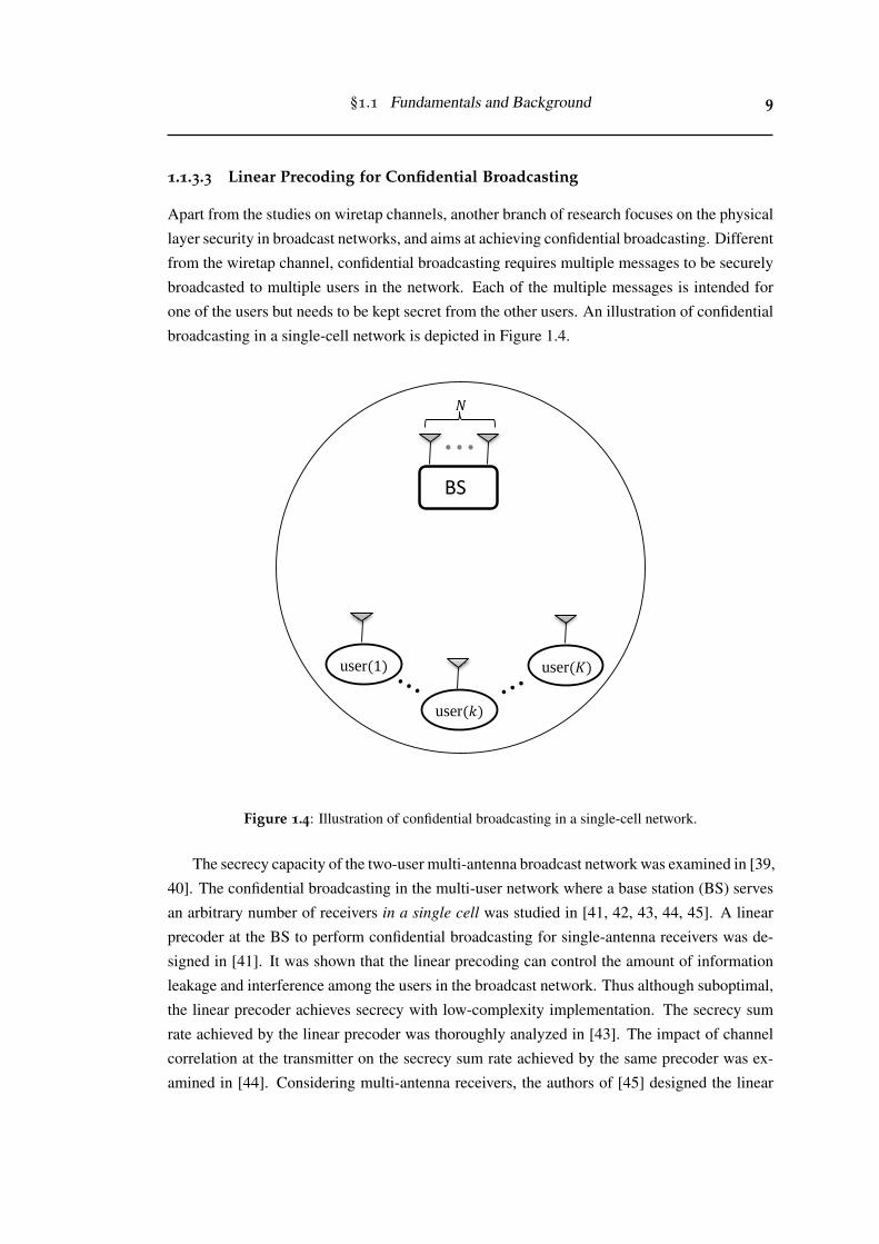
Apart from the studies on wiretap channels, another branch of research focuses on the physical
layer security in broadcast networks, and aims at achieving confidential broadcasting. Different
from the wiretap channel, confidential broadcasting requires multiple messages to be securely
broadcasted to multiple users in the network. Each of the multiple messages is intended for
one of the users but needs to be kept secret from the other users. An illustration of confidential
broadcasting in a single-cell network is depicted in Figure 1.4.
𝑁
⋯ BS
user(𝐾)
Type equation here. user(𝑘)
user(1)
𝑁
⋯
BS(2)
Cell 2
user(𝐾, 2)
Type equation here. user(𝑘, 2)
user(1,2)
𝒉𝑘,2,2
𝒉𝑘,2,1
Figure 1.4: Illustration of confidential broadcasting in a single-cell network.
The secrecy capacity of the two-user multi-antenna broadcast network was examined in [39,
40]. The confidential broadcasting in the multi-user network where a base station (BS) serves
an arbitrary number of receivers in a single cell was studied in [41, 42, 43, 44, 45]. A linear
precoder at the BS to perform confidential broadcasting for single-antenna receivers was de-
signed in [41]. It was shown that the linear precoding can control the amount of information
leakage and interference among the users in the broadcast network. Thus although suboptimal,
the linear precoder achieves secrecy with low-complexity implementation. The secrecy sum
rate achieved by the linear precoder was thoroughly analyzed in [43]. The impact of channel
correlation at the transmitter on the secrecy sum rate achieved by the same precoder was ex-
amined in [44]. Considering multi-antenna receivers, the authors of [45] designed the linear
10 Introduction
precoder to perform confidential broadcasting and addressed unequal distances from the BS to
the users.
1.2 Motivation and Challenges
Despite a significant amount of work that has been conducted from the theoretical perspective,
physical layer security is still far from actual implementations in practical networks, arguably
due to the impractical assumptions and the limited applicability.
1.2.1 Impractical Assumptions
As mentioned before, physical layer security is achieved by exploiting the characteristics
of wireless channels, such as fading, interference, and noise. Consequently, the level of
information-theoretic security provided by physical layer security techniques highly depends
on the knowledge of wireless channels which includes the knowledge about both the intended
receiver and the eavesdropper. Unfortunately, the assumption on the available knowledge is
not generally practical in many of existing literatures.
For instance, some existing articles assumed that the perfect CSI of the channels to the
intended receiver and the eavesdropper is available. Usually, the CSI is obtained at the receiver
by channel estimation during pilot transmission. Then, a feedback link (if available) is used to
send the CSI to the transmitter. In practice, an external eavesdropper naturally does not coop-
erate with the transmitter to send CSI feedback, and hence, it is very difficult for the transmitter
to obtain the CSI of the eavesdropper. Although the intended receiver may cooperate to send
CSI feedback, reliable uplink channels for the feedback cannot always be guaranteed. This
leads to an increasing amount of recent work focusing on the scenario where the transmitter
does not have perfect CSI of the channel to the intended receiver and/or the eavesdropper,
e.g., [31, 37, 46, 47, 48].
On the other hand, most existing studies still assumed that the intended receiver has perfect
CSI. Clearly, the assumption of perfect CSI available at the receiver is not very practical, since
the channel estimation at the receiver generally is not error-free. In principle, the channel
estimation error exists at both the intended receiver and the eavesdropper. Assuming perfect
estimation at the eavesdropper is relatively reasonable from the secure transmission design
point of view, since it is often difficult or impossible for the transmitter to know the accuracy
of the eavesdropper’s channel estimate. Assuming perfect CSI at the eavesdropper can be
regarded as a worst-case scenario for the analysis. However, the assumption of perfect CSI at
the intended receiver is difficult to justify from the practical perspective.
Apart from the assumption of perfect CSI knowledge at the receiver, another idealized
assumption is often adopted in the existing literature on physical layer security. That is, the
§1.2 Motivation and Challenges 11
number of eavesdropper antennas or an upper bound on the number of eavesdropper anten-
nas is assumed to been known at the legitimate side, e.g., [27, 28, 37, 49, 50, 51, 52, 53]. If
the number of eavesdropper antennas is unknown, we have to assume that the eavesdropper
has an infinite number of antennas as a worst-case consideration, and then the secrecy rate
would always go to zero intuitively. To the best of our knowledge, no existing literature has
studied the scenario where the number of eavesdropper antennas is totally unknown. In prac-
tice, an external eavesdropper naturally does not inform the legitimate side about the number
of antennas to expose its ability. As a weak justification, the upper bound on the number of
eavesdropper antennas could be estimated from the eavesdropper’s device size. However, such
a weak justification, probably valid in the past, can no longer hold with the current develop-
ment of large-scale antenna array technologies which allow a fast growing number of antennas
be placed within a limited space. Thus, how to characterize the performance of physical layer
security without knowing the number of eavesdropper antennas is a challenging but important
problem.
1.2.2 Limited Applicability
As the traditional approach to securing wireless communications, cryptographic techniques
have been well studied and designed for different systems subject to practical secrecy require-
ments. In contrast, the existing research on physical layer security is applicable only to sim-
plified systems with information-theoretic secrecy requirements. In other words, the existing
analysis on physical layer security is not generally applicable to practical wireless systems with
practical secrecy requirements.
We can see that the existing analysis on physical layer security is not generally applicable
for practical wireless systems by taking an example of the research on broadcast network with
confidential information. While the confidential broadcasting in a single isolated cell has been
elaborately studied, the solution to confidentially broadcasting messages in multi-cell networks
has not been addressed in the literature. In other words, the existing analysis on physical layer
security for achieving confidential broadcasting is applicable only for the networks with a
single isolated cell, but is not applicable for practical wireless networks with multiple cells not
far away from each other. The primary challenge to achieve confidential broadcasting in the
multi-cell network is to deal with the inter-cell information leakage and interference, besides
the intra-cell information leakage and interference. Thus, the techniques achieving single-
cell confidential broadcasting in existing research cannot be applied to achieving multi-cell
confidential broadcasting.
We now explain why the existing research on wireless physical layer security is not gen-
erally applicable for systems with practical secrecy requirements. The reason is due to the
fundamental limitations on the secrecy metrics that adopted by the existing studies. As intro-
12 Introduction
duced in Section 1.1.2, the secrecy performance of wireless transmissions over fading channels
is often measured by the ergodic secrecy capacity or the secrecy outage probability. Unfortu-
nately, these two secrecy measures are not (closely) related to the secrecy requirements in
practice, and do not bear the same significance from a cryptographic perspective. In particular,
the current definition of secrecy outage probability has two major limitations in evaluating the
secrecy performance of wireless systems. First, the secrecy outage probability does not give
any insight into the eavesdropper’s ability to decode the confidential messages. The eaves-
dropper’s decodability is an intuitive measure of security in real-world communication systems
when classical information-theoretic secrecy is not always achievable, and error-probability-
based secrecy metrics are often adopted to quantify secrecy performance in the literature,
e.g., [54, 55, 56, 57]. A general secrecy requirement for the eavesdropper’s decoding error
probability, Pe, can be given as Pe ≥ ϑ , where 0 < ϑ ≤ 1 denotes the minimum acceptable
value of Pe. In contrast, classical secrecy outage probability reflects only an extremely strin-
gent requirement on Pe for ϑ → 1, i.e., requiring ϑ → 1, since classical information-theoretic
secrecy guarantees Pe → 1. Second, the amount of information leakage to the eavesdropper
cannot be characterized. When classical information-theoretic secrecy is not achievable, some
information will be leaked to the eavesdropper. Different secure transmission designs that lead
to the same secrecy outage probability may actually result in very different amounts of infor-
mation leakage. Consequently, it is important to know how much or how fast the confidential
information is leaked to the eavesdropper to obtain a finer view of the secrecy performance.
However, the classical outage-based approach is not able to evaluate the amount of information
leakage when a secrecy outage occurs.
1.3 Thesis Outline and Contributions
The objective of the thesis is to make contributions for bridging the gap between theory and
practice in physical layer security. To reduce the dependence of physical layer security on
impractical assumptions, we study the on-off transmission design with the consideration of
channel estimation errors in Chapter 2, and provide an innovative solution to the challenging
problem of achieving secrecy without knowing the number of eavesdropper antennas in Chap-
ter 3. To make the analysis on physical layer security more applicable in practical networks, we
develop an effective solution to tackle the challenge of confidential broadcasting in multi-cell
networks in Chapter 4, and propose new secrecy measures for wireless systems over fading
channels in Chapter 5. The contributions of each chapter are emphasized as follows.
§1.3 Thesis Outline and Contributions 13
Chapter 2 – Secure On-Off Transmission Design with Channel EstimationErrors
Chapter 2 studies the impact of channel estimation errors on the secure on-off transmission
design. As introduced in Section 1.1.3.1, the secure on-off transmission scheme [16, 19] is
an important secrecy enhancement for improving the secrecy performance of single-antenna
wireless systems. The main contributions of this chapter are summarized as follows:
• We consider quasi-static slow fading channels and use the secrecy outage probability to
study the secure transmission design with channel estimation errors at the receiver side.
This is different from the previous works considering the impact of imperfect channel
estimations on physical layer security, which all used the ergodic secrecy rate as the
performance measure.
• We develop throughput-maximizing secure on-off transmission schemes with fixed en-
coding rates for different scenarios distinguished on whether or not there is channel es-
timation error at the eavesdropper, and whether or not the transmitter has the estimated
channel quality fed back from the eavesdropper. Our analytical and numerical results
show how the optimal design and the achievable throughput vary with the change in the
channel knowledge assumptions.
• For systems in which the encoding rates are controllable parameters to design, we jointly
optimize the encoding rates and the on-off transmission thresholds to maximize the
throughput of secure transmissions. Both non-adaptive and adaptive rate transmissions
are considered. Note that none of the previous works on physical layer security consid-
ering the channel estimation error has explicitly involved the rate parameters as part of
the design problem.
• We also analyze how the training (pilot) power affects the achievable throughput of
secure transmissions, since the accuracy of the channel estimation depends on the pilot
power. One interesting finding is that, in the scenario where both the intended receiver
and the eavesdropper obtain imperfect channel estimates, increasing the pilot power for
more accurate channel estimation can harm the throughput of the secure transmission
even if the pilot power is obtained for free.
The results in this chapter have been presented in the following publications which are
listed again for ease of reference:
J1. B. He and X. Zhou, “Secure on-off transmission design with channel estimation errors,"
IEEE Trans. Inf. Forensics Security, vol. 8, no. 12, pp. 1923–1936, Dec. 2013.
C1. B. He and X. Zhou, “Impact of channel estimation error on secure transmission design,”
in Proc. IEEE AusCTW, Adelaide, SA, Jan. 2013, pp. 19–24.
14 Introduction
Chapter 3 – Achieving Secrecy without Knowing the Number of Eavesdrop-per Antennas
In Chapter 3, we provide an innovative solution to the challenging problem of how to achieve
secrecy without the impractical assumption of knowing the number of eavesdropper antennas.
Specifically, we introduce the concept of spatial constraint into physical layer security. Here
the spatial constraint means the limited size of the spatial region for placing antennas at the
communication node. In practice, knowing the eavesdropper’s spatial constraint for placing
antennas is much easier than knowing the exact number of the eavesdropper antennas. For
example, we may know the size of the eavesdropper’s device, but it is difficult to know how
many antennas are installed on the device. Also, we may know that the eavesdropper hides in
a room, but it is difficult to known how many antennas are placed inside the room.
The primary contributions of this chapter are summarized as follows.
• We introduce spatial constraints into physical layer security. To this end, we propose a
framework to study physical layer security in multi-antenna systems with spatial con-
straints at the receiver side (both the intended receiver and the eavesdropper). We derive
the secrecy capacity, and analyze the impact of spatial constraints on the secrecy capac-
ity.
• For the first time, our proposed framework allows one to analyze physical layer se-
curity without the knowledge of the number of eavesdropper antennas. It relaxes the
requirement on the knowledge of eavesdropper from knowing the number of antennas to
knowing the spatial constraint. We show that a non-zero secrecy capacity is achievable
even if the eavesdropper is assumed to have an infinite number of antennas. This is eas-
ily achieved by applying the basic friendly-jamming technique where the jammer sends
random noise signals.
• We further study the impact of jamming power on the secrecy capacity of the spatially-
constrained jammer-assisted systems. For the basic jammer-assisted system, we find
that the secrecy capacity does not monotonically increase with the jamming power, and
we obtain the closed-form solution of the optimal jamming power that maximizes the
secrecy capacity. The optimality of the obtained solution is confirmed by the numerical
result.
The results in this chapter have been presented in the following publications which are
listed again for ease of reference:
J3. B. He, X. Zhou, and T. D. Abhayapala, “Achieving secrecy without knowing the number
of eavesdropper antennas," IEEE Trans. Wireless Commun., vol. 14, no. 12, pp. 7030–
7043, Dec. 2015.
§1.3 Thesis Outline and Contributions 15
Chapter 4 – Base Station Cooperation for Confidential Broadcasting in Multi-Cell Networks
In Chapter 4, we build up an effective solution to tackle the challenge of confidential broad-
casting in multi-cell networks. In the network, BS cooperation [58] is taken into consideration
such that the BSs can share control signals, CSI and/or messages to cooperatively serve users
in multiple cells. With BS cooperation, we specifically consider the confidential broadcasting
in a symmetric two-cell network where there are K single-antenna users and one N-antenna
BS in each cell. The two BSs cooperatively broadcast confidential information to the users.
We focus on two different forms of cooperation at the BSs: i) multi-cell processing (MCP) and
ii) coordinated beamforming (CBf). In the MCP, the BSs fully cooperate such that they share
their CSI and messages to transmit. Alternatively, in the CBf the BSs “partially” cooperate. As
such, they do not share their messages to transmit but allow users to feed back the CSI to the
cross-cell BS.
The primary contributions of this chapter are summarized as follows.
• We design a linear precoder as per the principles of regularized channel inversion (RCI) [59]
to perform confidential broadcasting in the multi-cell network with the MCP.1 We also
design a linear precoder as per the principles of generalized RCI [60] to perform con-
fidential broadcasting in the multi-cell network with the CBf. In each precoder, the
precoding matrix is designed to trade off the intended received signal, the intra- and
inter-cell information leakage, and the intra- and inter-cell interference via a regulariza-
tion parameter.
• We derive new channel-independent expressions for the secrecy sum rate achieved by
the designed linear precoders for both the MCP and the CBf in the large-system regime.
In this regime, we consider K,N→ ∞ and keep the ratio β = K/N constant. The large-
system expressions do not depend on the channel realizations, and thus eliminate the
computational burden of performance evaluation incurred by Monte Carlo simulations.
Notably, numerical results confirm that our large-system expressions are accurate even
for finite K and N.
• We optimize the secrecy performance of confidential broadcasting in the multi-cell net-
work based on our large-system expressions. We first determine the optimal regulariza-
tion parameters of the RCI and the generalized RCI precoders in order to maximize the
secrecy sum rate for the MCP and the CBf, respectively. We then design power-reduction
linear precoders in order to significantly increase the secrecy sum rate at high transmit
SNRs when the network load is high. To do this, we propose power-reduction strategies
for the MCP when β > 1 and the CBf when β > 0.5. These strategies effectively prevent
1The RCI is also sometimes called as regularized zero forcing (RZF) in some literatures.
16 Introduction
the the secrecy sum rate from decreasing at high transmit SNRs which is caused by the
RCI precoder when β > 1 and the generalized RCI precoder when β > 0.5.
The results in this chapter have been presented in the following publications which are
listed again for ease of reference:
J2. B. He, N. Yang, X. Zhou, and J. Yuan, “Base station cooperation for confidential broad-
casting in multi-cell networks," IEEE Trans. Wireless Commun., vol. 14, no. 10, pp.
5287–5299, Oct. 2015.
C3. B. He, N. Yang, X. Zhou, and J. Yuan, “Confidential broadcasting via coordinated beam-
forming in two-cell networks,” in Proc. IEEE ICC, London, UK, June 2015, pp. 7376–
7382.
Chapter 5 – New Secrecy Measures for Wireless Transmissions over FadingChannels
In Chapter 5, we propose three new secrecy metrics for wireless transmissions focusing on
quasi-static fading channels, motivated by the limitations of the secrecy outage probability in
evaluating practical networks. We evaluate the secrecy performance of an example wireless
system with fixed-rate wiretap codes to illustrate the use of the proposed secrecy metrics, and
show that the proposed secrecy metrics can jointly give a more comprehensive and in-depth
understanding of the secrecy performance of wireless transmission over fading channels. We
find that the newly proposed secrecy metrics lead to very different optimal design parameters
that optimize the secrecy performance of the system, compared with the optimal design min-
imizing the current secrecy outage probability. Applying the optimal design that minimizes
the secrecy outage probability can result in a large secrecy loss, if the actual system requires
a low decodability at the eavesdropper and/or a low information leakage rate. The primary
contributions of this chapter, i.e., the three new secrecy metrics, are summarized as follows.
• Extended from the current definition of secrecy outage, a generalized formulation of
secrecy outage probability is proposed. The generalized secrecy outage probability takes
into account the level of secrecy measured by equivocation, and hence establishes a link
between the existing concept of secrecy outage and the decodability of messages at the
eavesdropper.
• An asymptotic lower bound on the eavesdropper’s decoding error probability is pro-
posed. This proposed metric provides a direct error-probability-based secrecy metric
that is typically used for the practical implementation of actual secure wireless systems
over fading channels.
§1.3 Thesis Outline and Contributions 17
• A metric evaluating the average information leakage rate is proposed. This proposed
secrecy metric gives an answer to the important question of how fast or how much
the confidential information is leaked to the eavesdropper when perfect secrecy is not
achieved.
The results in this chapter have been presented in the following publications which are
listed again for ease of reference:
J4. B. He, X. Zhou, and A. L. Swindlehurst, “On secrecy metrics for physical layer security
over quasi-static fading channels," submitted to IEEE Trans. Wireless Commun., Jan.
2016.
C2. B. He and X. Zhou, “New physical layer security measures for wireless transmissions
over fading channels,” in Proc. IEEE GLOBECOM, Austin, TX, Dec. 2014, pp. 722–
727.

18 Introduction
Chapter 2
Secure On-Off Transmission Designwith Channel Estimation Errors
2.1 Introduction
One of the key features in providing physical layer security is that the CSI of both the legitimate
receiver and the eavesdropper often needs to be known by the transmitter to enable secure
encoding and advanced signaling. However, the assumption of perfectly knowing the CSI is
almost impossible in practice. This chapter aims to reduce the dependence of physical layer
security on the impractical assumption of perfect CSI. Specifically, we study the impact of
channel estimation errors on secure on-off transmissions designs.
In recent years, increasing attention has been paid to the impact of the uncertainty in the
CSI of both legitimate receiver and eavesdropper’s channels at the transmitter, e.g., [31, 37,
46, 47, 48]. Usually, the CSI is obtained at the receiver by channel estimation during pilot
transmission [61]. Then, a feedback link (if available) is used to send the CSI to the trans-
mitter. Hence, the accuracy of the channel estimation at the receiver affects the quality of
CSI at the transmitter. In the literature of physical layer security, most existing studies as-
sumed that the legitimate receiver has perfect channel estimation. Clearly, this assumption is
not practical, since the channel estimation problem usually is not error-free. Previous stud-
ies on the physical layer security considering the imperfect channel estimation at the receiver
side can be found in [28, 36, 38], where [28, 36] considered the channel estimation error at
the legitimate receiver and [38] considered the channel estimation error at both the legitimate
receiver and the eavesdropper. Specifically, Taylor et al. presented the impact of the legiti-
mate receiver’s channel estimation error on the performance of an eigenvector-based jamming
technique in [36]. Their research showed that the ergodic secrecy rate provided by the jam-
ming technique decreases rapidly as the channel estimation error increases. Zhou and McKay
analyzed the optimal power allocation of the AN for the secure transmission considering the
impact of imperfect CSI at the legitimate receiver in [28]. They found that it is wise to create
more AN by compromising on the transmit power of information-bearing signals when the CSI
19
20 Secure On-Off Transmission Design with Channel Estimation Errors
is imperfectly obtained. Liu et al. [38] adopted the secrecy beamforming scheme to investigate
the joint design of training and data transmission signals for wiretap channels. They derived
the ergodic secrecy rate for practical systems with imperfect channel estimations at both the
legitimate receiver and the eavesdropper, and found the optimal tradeoff between the energy
used for training and data signals based on the achievable ergodic secrecy rate.
The aforementioned works in [28, 36, 38] all used the ergodic secrecy rate to characterize
the performance limits of systems. The ergodic secrecy rate is an appropriate secrecy metric
for systems in which the encoded messages span sufficient channel realizations to capture the
ergodic features of the fading channel [16]. In addition, the works in [28, 36, 38] implicitly
assumed variable-rate transmission strategies where the encoding rates are adaptively chosen
according to the instantaneous channel gains. The system achieving the ergodic secrecy rate
has the implicit assumption of the variable-rate transmission, which is very different from
traditional ergodic fading scenarios without the secrecy consideration. A detailed explanation
can be found in [16]. In practice, communication systems sometimes prefer non-adaptive
rate transmission to reduce complexity and applications like video streams in multimedia often
require fixed encoding rates. Thus, variable-rate transmission strategies are not always feasible.
The remainder of this chapter is organized as follows. Section 2.2 gives the system model
and the assumptions on channel knowledge. Section 2.3 analyzes the secure on-off trans-
mission design for systems with fixed encoding rates. Section 2.4 develops two joint rate
and on-off transmission designs depending on whether the encoding rates are non-adaptive or
adaptive.1 Numerical results and the summary of this chapter are given in Sections 2.5 and 2.6,
respectively.
2.2 System Model
We consider a three-node wireless network in which a transmitter, Alice, wants to send confi-
dential information to an intended user, Bob, in the presence of an eavesdropper, Eve. Alice,
Bob and Eve are assumed to have a single antenna each. Both Bob and Eve are mobile users
served by the BS, Alice. In order to secure the transmission to Bob against Eve, Alice tracks
the channel qualities of both mobile stations by asking them to feed back their estimated in-
stantaneous channel qualities through error-free feedback links. Note that only the channel
quality, which is a real number as opposed to the complex channel coefficient, is required to
feed back to Alice.
The main assumptions on the system model made in this chapter are listed as follows.
(a) We assume quasi-static fading channels and adopt the block fading model [62], where
1The system with non-adaptive rates in Section 2.4 is different from the system with fixed rates in Section 2.3.The fixed rates indicate that the encoding rates are given and cannot be chosen freely, while the non-adaptive ratesindicate that the encoding rates can be chosen in the design process but are constant for all message transmissions.
§2.2 System Model 21
the channel gains remain constant over a block of symbols (i.e., the transmission of one
message) and change independently from one block to the next.
(b) The block-wise transmission is adopted. At the start of each block, pilot symbols are
transmitted to enable channel estimation at the receiver. Then, both Bob and Eve estimate
their channels and feed the estimated channel qualities back to Alice. Finally, the data
symbols are transmitted.
(c) We assume that the transmission power of the pilot symbol can be different from the trans-
mission power of the data symbol.
(d) We assume that the duration of a block is sufficiently long. For simplicity, the time spent
on training and feedback is negligible compared with the data transmission time.
(e) We assume that the average SNRs at both Bob and Eve, without the consideration of
channel estimation errors, are known at Alice.
The data symbol transmitted by Alice is denoted by d. The transmission power of the data
symbol is normalized so that E{|d|2}= 1. The pilot symbol is denoted by t. The ratio of pilot
power to data power is denoted by
ψ =E{|t|2}E{|d|2}
= E{|t|2}. (2.1)
Since E{|d|2}= 1, we call ψ as the normalized pilot power (normalized by data power). The
received symbols at Bob and Eve are given by
yb =√
αbhbx+ nb (2.2)
and
ye =√
αehex+ ne, (2.3)
respectively, where hb ∼ CN (0,1) and he ∼ CN (0,1) denote the normalized channel gain
from Alice to Bob and the normalized channel gain from Alice to Eve, respectively. We as-
sume that hb and he are independent. This assumption is reasonable for rich-scattering envi-
ronment where Bob and Eve are not very close to each other. The additive white Gaussian
noise (AWGN) at Bob is denoted by nb ∼ CN (0,1) and the AWGN at Eve is denoted by
ne ∼ CN (0,1). The transmitted signal x can be a data symbol, d, or a pilot symbol, t. We fur-
ther assume that the data power is normalized to unity, i.e., E{|x|2}= 1. The average (data)
SNRs at Bob and Eve without the consideration of channel estimation errors are denoted by
αb and αe, respectively. In fact, αb and αe indicate the overall channel conditions between the
transmitter and the receivers. For example, αb > αe may indicate that the distance between
Alice and Bob is smaller than the distance between Alice and Eve.
22 Secure On-Off Transmission Design with Channel Estimation Errors
2.2.1 Channel Estimation
We assume that Bob’s channel is estimated by the minimum mean square error (MMSE) esti-
mator during pilot transmission. The estimation of Bob’s channel gain and the estimation error
are denoted by hb and hb, respectively. Thus,
hb = hb + hb, (2.4)
where hb and hb are assumed to have zero-mean complex Gaussian distributions. The assump-
tion of Gaussian distributed channel estimation error arises from the use of MMSE estimator
for channel estimation in the Bayesian linear model [63], e.g., the pilot-symbol-aided channel
estimation [64]. More specifically, since the channel coefficient, hb, has a complex Gaussian
distribution and the received signal, yb, is a linear function of the channel coefficient, the linear
MMSE estimation becomes the optimal MMSE estimation. Thus, by using a linear estimator,
the estimated channel coefficient and the estimation error are zero-mean complex Gaussian
distributed. In fact, |hb| is what Bob feeds back to Alice as the estimated instantaneous chan-
nel quality. The orthogonality principle implies E{|hb|2} = E{|hb|2}+E{|hb|2}. According
to [65], the variance of channel estimation error is given by
ςb = E{|hb|2}=1
1+ψαbTt, (2.5)
where Tt is the length of pilot transmission. We assumed that Tt = 1. Hence the effect of
channel training is solely characterized by the normalized pilot power, ψ . For convenience, we
let γb = αb|hb|2 and γb = αb|hb|2, each having an exponential distribution given by
fγb(γb) =1
αb(1− ςb)exp(− γb
αb(1− ςb)
), γb > 0, (2.6)
fγb(γb) =1
αbςbexp(− γb
αbςb
), γb > 0. (2.7)
Bob uses the estimated channel gain for data detection, and the actual instantaneous SNR at
Bob can be written as [66]
γb =αb|hb|2
αb|hb|2 + 1=
γb
γb + 1. (2.8)
We assume that Eve’s channel is also estimated by the MMSE estimator. The estimation of
Eve’s channel gain and the estimation error are denoted by he and he, respectively. Thus,
he = he + he. (2.9)
Under the assumption of MMSE estimator for channel estimation in the Bayesian linear model,
he and he have zero-mean complex Gaussian distributions. In fact, |he| is what Eve is required
§2.2 System Model 23
to feed back to Alice as the estimated instantaneous channel quality. The orthogonality prin-
ciple implies E{|he|2}= E{|he|2}+E{|he|2}. In addition, the variance of channel estimation
error is given by
ςe = E{|he|2}=1
1+ψαeTt, (2.10)
where we assume that Tt = 1. Similarly, we let γe = αe|he|2 and γe = αe|he|2, each having an
exponential distribution given by
fγe(γe) =1
αe(1− ςe)exp(− γe
αe(1− ςe)
), γe > 0, (2.11)
fγe(γe) =1
αeςeexp(− γe
αeςe
), γe > 0. (2.12)
With the MMSE channel estimation, the actual instantaneous SNR for data detection at Eve
can be written as
γe =αe|he|2
αe|he|2 + 1=
γe
γe + 1. (2.13)
It is worth mentioning that in principle Eve is able to further improve the channel estimation by
performing joint channel and data detection, while Alice has no mechanism to tell if this is the
case. As a robust approach for achieving secrecy, Alice may assume the worst case scenario
where Eve perfectly knows her own channel. Then, the actual instantaneous SNR at Eve is
γe = αe|he|2, which has an exponential distribution given by
fγe(γe) =1
αeexp(− γe
αe
), γe > 0. (2.14)
2.2.2 Channel Knowledge
As mentioned before, Alice asks both Bob and Eve to feed back their estimated instantaneous
channel qualities after the pilot transmission phase. Since Bob is the intended user, we simply
assume that Alice has and trusts the feedback from Bob with the knowledge of γb = αb|hb|2
as Bob’s estimated instantaneous SNR. The actual instantaneous SNR at Bob is given in (2.8).
However, Eve is an eavesdropper, and may not cooperate with Alice. Hence, Alice may not
obtain or trust the feedback information from Eve. We specifically investigate the following
three scenarios with different assumptions on the channel knowledge:
• Scenario 1: Alice has and trusts the feedback from Eve, knowing γe = αe|he|2 as the
estimate of the instantaneous SNR at Eve. Eve uses the MMSE channel estimate he for
data detection, and hence the actual instantaneous SNR at Eve is given in (2.13).
• Scenario 2: Alice has and trusts the feedback from Eve, knowing γe = αe|he|2 as the
24 Secure On-Off Transmission Design with Channel Estimation Errors
estimate of the instantaneous SNR at Eve. Eve is assumed to perfectly know her own
channel, and the actual instantaneous SNR at Eve is γe = αe|he|2.
• Scenario 3: Alice does not have or trust Eve’s feedback, and hence has no knowledge
about Eve’s instantaneous channel. However, the statistics of Eve’s channel, i.e., αe, is
still assumed to be known at Alice. Eve perfectly knows her own channel, and the actual
instantaneous SNR at Eve is γe = αe|he|2.
In fact, the three scenarios above can also be interpreted as follows. Scenario 1 represents
the case where Eve is exactly identical to other mobile users. Scenario 2 generally represents
the case where Alice has partial information about Eve’s channel gain, while allowing Eve
to have perfect knowledge on her own channel. Scenario 3 is valid for the case where Alice
has no feedback from Eve. This scenario is perhaps the most practical one with current com-
munication protocols where the channel feedback is only obtained from the intended receiver.
Scenario 3 is also a robust approach for secrecy that allows Eve to have malicious behaviors,
e.g., feeding wrong information back to Alice.
We note that Scenario 2 is the least-practical amongst the three scenarios. It is worth
highlighting the value of studying Scenario 2 in this chapter. From the legitimate users’ per-
spectives, Scenario 1 represents the most desirable case, where Alice has the feedback from
Eve and Eve has imperfect CSI. In contrast, Scenario 3 represents the worst case, where Alice
has no feedback from Eve and Eve has perfect CSI. There are two different CSI assumptions
between these two scenarios, one on the feedback from Eve to Alice and the other on the CSI
knowledge at Eve. From theoretical point of view, it is meaningful to evaluate the impact of
changing one of the CSI assumptions on the secure transmission design. To this end, Sce-
nario 2 is introduced as it differs from Scenario 1 or 3 in only one CSI assumption. The study
of Scenario 2 enables us to compare the secure transmissions with different CSI assumptions
changing in step. Specifically, we can learn the effect of the having different CSI qualities
at Eve by comparing Scenarios 1 and 2. We can find the impact of the availability of CSI
feedback at Alice by comparing Scenarios 2 and 3.
2.2.3 Secure Encoding
We consider the widely-adopted wiretap code [13] as introduced in Section 1.1.1 for the mes-
sage transmissions. The two rate parameters are the codeword transmission rate, Rb, and the
confidential information rate, Rs. The positive rate difference Re =Rb−Rs is the cost to provide
secrecy against the eavesdropper. From [13] [67, Theorem 1] [68, Definition 2], perfect secrecy
cannot be achieved when Re <Ce, where Ce denotes Eve’s channel capacity, Ce = log2(1+γe).
Also, Bob is unable to decode the received codewords correctly when Rb > Cb, where Cb de-
notes Bob’s channel capacity, Cb = log2(1+ γb). Thus, given a pair of the rate choices, Rb
§2.3 On-Off Transmission Design 25
and Rs, the secrecy outage probability [19], pso, and the connection outage probability, pco, are
given as
pso = P(Ce > Rb−Rs |message transmission), (2.15)
pco = P(Cb < Rb |message transmission). (2.16)
Note that both outage probabilities are conditioned on the message transmission. The secrecy
level and the reliability level of a transmission scheme can then be measured by the secrecy
outage probability and the connection outage probability, respectively.
2.3 On-Off Transmission Design
In the following, we consider each of the three scenarios described in Section 2.2 and show
how to design transmission schemes with good throughput performance, whilst satisfying the
secrecy and reliability constraints. In particular, we consider the on-off transmission scheme:
Alice decides whether or not to transmit according to the information about Bob and Eve’s
estimated instantaneous SNRs, i.e., transmission takes place when the estimated instantaneous
SNR at Bob, γb, is greater than a certain threshold, µb, and the estimated instantaneous SNR
at Eve, γe, is less than another threshold, µe, while transmission is suspended when γb ≤ µb
or γe ≥ µe. Since the secrecy and reliability performances are related to different channels,
which can be seen from (2.15) and (2.16), it is reasonable to set two separate SNR thresholds
on Bob’s channel and Eve’s channel, respectively. In the scenario where Alice does not have
or trust the feedback from Eve, there is no on-off SNR threshold on Eve’s channel, µe, or
equivalently µe = ∞.
We assume that the encoding rates have already been designed such that both the codeword
transmission rate, Rb, and the confidential information rate, Rs, are fixed. The design problem
is to maximize the throughput, η , subject to two constraints, one on the secrecy performance
and the other on the reliability performance, which can be written as
maxµb,µe
η = ptx (1− pco)Rs, (2.17)
s.t. pso ≤ ϕ , pco ≤ δ , (2.18)
where ptx denotes the probability of transmission due to the on-off transmission scheme,
ϕ ∈ [0,1] and δ ∈ [0,1] represent the secrecy and reliability requirements. The maximum
acceptable secrecy outage probability is ϕ , and the maximum acceptable connection outage
probability is δ . The controllable parameters to design are the two on-off SNR thresholds, µb
and µe.
Note that the overhead of pilot and feedback is not considered for calculating the through-
put in (2.17), since we assume a sufficiently long block length for simplicity. If the pilot
26 Secure On-Off Transmission Design with Channel Estimation Errors
transmission and feedback time is considered, we can simply introduce a new parameter, say
ϖ , to represent the ratio of pilot transmission and feedback time to data transmission time.
Then, the throughput can be calculated by taking this ratio, ϖ , into account, i.e., (2.17) will
change to η = 11+ϖ
ptx(1− pco)Rs.
In what follows, we consider the transmission design in the three different scenarios de-
scribed in Section 2.2. For each scenario, the transmission probability, the connection outage
probability and the secrecy outage probability are derived firstly. Then, the feasibility of se-
crecy and reliability constraints is discussed. Here the feasibility of constraints means that the
constraints can be satisfied whilst achieving a positive information rate. Finally, the solution
of the optimization problem is given as a proposition.
2.3.1 Scenario One
Derivations of ptx, pco and pso: Since Bob’s estimated instantaneous SNR is independent with
Eve’s estimated instantaneous SNR, the probability of transmission in Scenario 1 is given as
ptx = P(γb > µb)P(γe < µe)
= exp(− µb
αb(1− ςb)
)(1− exp
(− µe
αe(1− ςe)
)). (2.19)
Since γb ≤ γb according to (2.8) and Bob can decode the message without error only when
Cb ≥ Rb, it is wise to choose the value of µb satisfying
log2(1+ µb) ≥ Rb⇒ µb ≥ 2Rb−1. (2.20)
Then, the connection outage probability in Scenario 1 is given by
pco = P (log2(1+ γb) < Rb | γb > µb)
= P
(log2
(1+
γb
γb + 1
)< Rb | γb > µb
)=
P(µb < γb < (2Rb−1)(γb + 1))P(γb > µb)
= exp(
µb
αb(1− ςb)
)∫∞
µb2Rb−1
−1
(∫ (2Rb−1)(γb+1)
µb
fγb(γb)dγb
)fγb(γb)dγb
=ςb(2Rb−1)
1+ ςb(2Rb−2)exp(
1αbςb
(1− µb
2Rb−1
)). (2.21)
§2.3 On-Off Transmission Design 27
The secrecy outage probability in Scenario 1 is given by
pso = P(Ce > Rb−Rs | γe < µe)
= P
(log2
(1+
γe
γe + 1
)> Rb−Rs | γe < µe
)=
P((2Rb−Rs−1)(γe + 1) < γe < µe
)P(γe < µe)
. (2.22)
If µe ≤ 2Rb−Rs−1, we get pso = 0. If µe > 2Rb−Rs−1, we have
pso =
∫ µe2Rb−Rs−1
−1
0
(∫ µe
(2Rb−Rs−1)(γe+1)fγe(γe)dγe
)fγe(γe)dγe
1− exp(− µe
αe(1−ςe)
)=
1−ςe1+ςe(2Rb−Rs−2) exp
(−2Rb−Rs−1
αe(1−ςe)
)− exp
(− µe
αe(1−ςe)
)1− exp
(− µe
αe(1−ςe)
)+
ςe(2Rb−Rs−1)1+ςe(2Rb−Rs−2) exp
(1
αe
(1ςe− µe
1−ςe− µe
ςe(2Rb−Rs−1)
))1− exp
(− µe
αe(1−ςe)
) . (2.23)
From (2.21), we find that the value of the on-off SNR threshold on Bob’s channel needs to
be very large such that µb goes to infinity, if the reliability constraint is very stringent such that
pco is required to go to zero. When µb goes to infinity, the throughput η will approach zero.
Thus, it is interesting to investigate the behaviors of η and pco for the limiting case where µb
goes to infinity. From (2.17), (2.19) and (2.21), we see that both η and pco are exponential
functions of µb as µb goes to infinity. Then, the slopes of η and pco with respect to µb go to
zero as µb goes to infinity.
From (2.22) and (2.23), we find that the secrecy outage probability is directly influenced
by the value of µe but not related to µb. If µe ≤ 2Rb−Rs − 1, perfect secrecy is achievable in
Scenario 1. Since γe ≥ γe in Scenario 1, the estimate of Eve’s instantaneous SNR is an upper
bound of the actual Eve’s instantaneous SNR. Hence, Alice can make sure that Ce < Rb−Rs by
having µe ≤ 2Rb−Rs −1. According to (2.23), we also find that the secrecy outage probability
increases as µe increases if µe > 2Rb−Rs−1.
Feasibility of Constraints: From (2.21), we find that pco is a decreasing function of µb and
limµb→+∞
pco = 0. (2.24)
Thus, the feasible range of the reliability constraint in Scenario 1 is given by
0 < δ ≤ 1. (2.25)
28 Secure On-Off Transmission Design with Channel Estimation Errors
According to (2.22), pso is an increasing function of µe and pso = 0 as long as µe ≤ 2Rb−Rs−1.
Thus, the feasible range of the secrecy constraint in Scenario 1 is given by
0≤ ϕ ≤ 1. (2.26)
Hence, any required reliability and secrecy constraints are feasible by appropriately adjusting
the on-off thresholds. It is noted that perfect secrecy, i.e., ϕ = 0, can be achieved.
The following proposition summarizes the solution to the design problem in Scenario 1,
where the optimal µb is expressed in a closed form and the optimal µe is obtained by numeri-
cally solving an equation.
Proposition 2.1. The optimal parameters of the throughput-maximizing transmission scheme
in Scenario 1 are given as follows:
µb =
2Rb−1 , if Rb ≤ log2
(1+ (1−ςb)δ
ςb(1−δ )
)(2Rb−1
)(1−αbςb ln
(δ
1+ςb(2Rb−2)ςb(2Rb−1)
)), otherwise,
(2.27)
µe =
{+∞ , if 1−ςe
1+ςe(2Rb−Rs−2) exp(−2Rb−Rs−1
αe(1−ςe)
)≤ ϕ
F1 , otherwise,(2.28)
where F1 is the solution of µe to the equation
ϕ =
1−ςe1+ςe(2Rb−Rs−2) exp
(−2Rb−Rs−1
αe(1−ςe)
)− exp
(− µe
αe(1−ςe)
)1− exp
(− µe
αe(1−ςe)
)+
ςe(2Rb−Rs−1)1+ςe(2Rb−Rs−2) exp
(1
αe
(1ςe− µe
1−ςe− µe
ςe(2Rb−Rs−1)
))1− exp
(− µe
αe(1−ςe)
) . (2.29)
Proof: See Appendix A.1. �
Remark 2.1. In this scenario, if the transmitter increases the pilot power, the estimation er-
rors at both the legitimate receiver and the eavesdropper will reduce. Thus, the selection of
normalized pilot power, ψ , will create an interesting tradeoff between reducing the estimation
errors at the legitimate receiver and reducing the estimation errors at the eavesdropper. Here,
we briefly discuss the method to calculate the optimal ψ as follows, instead of providing a
detailed analysis. First, we need to find the expressions of optimal µb and µe in terms of ψ
by substituting (2.5) and (2.10) into (2.27) and (2.28), respectively. Then, ptx and pco can be
expressed as functions of ψ . Finally, the optimal ψ is the solution to the optimization problem
§2.3 On-Off Transmission Design 29
of
maxψ
η = ptx(ψ) (1− pco(ψ))Rs, (2.30)
s.t. ψ > 0. (2.31)
Due to the complicated expressions for the optimal µb and µe, the closed-form expression for
the optimal ψ is mathematically intractable. But this problem can be solved numerically.
2.3.2 Scenario Two
Derivations of ptx, pco and pso: The derivations of the probability of transmission and the con-
nection outage probability in Scenario 2 are the same as (2.19) and (2.21) in Scenario 1, re-
spectively. The secrecy outage probability in Scenario 2 is given by
pso = P(Ce > Rb−Rs | γe < µe)
= P(log2(1+ γe) > Rb−Rs | γe < µe)
=P(γe > 2Rb−Rs−1, γe < µe)
P(γe < µe)
=
∫ µe0
(∫∞
2Rb−Rs−1 fγe|γe(γe|γe)dγe)
fγe(γe)dγe
1− exp(− µe
αe(1−ςe)
) . (2.32)
According to the definitions of γe and γe in Scenario 2, γe conditioned on its estimate, γe,
follows a non-central chi-square distribution with two degrees of freedom. Applying the cu-
mulative distribution function of the non-central chi-square distribution, we have
∫∞
2Rb−Rs−1fγe|γe(γe|γe)dγe = Q1
(√2γe
αeςe,
√2Rb−Rs+1−2
αeςe
), (2.33)
where Qx(a,b) represents the Marcum Q-function [69]. Thus, the secrecy outage probability
in Scenario 2 can be rewritten as
pso =
∫ µe0 Q1
(√2γe
αeςe,√
2Rb−Rs+1−2αeςe
)fγe(γe)dγe
1− exp(− µe
αe(1−ςe)
)=
∫ µe0 exp
(− γe
αe(1−ςe)
)Q1
(√2γe
αeςe,√
2Rb−Rs+1−2αeςe
)dγe
αe (1− ςe)(
1− exp(− µe
αe(1−ςe)
)) . (2.34)
Feasibility of Constraints: Since the connection outage probability does not change from
Scenario 1 to Scenario 2, the feasible range of the reliability constraint in Scenario 2 is identical
30 Secure On-Off Transmission Design with Channel Estimation Errors
to (2.25) in Scenario 1. Since pso is an increasing function of µe and
limµe→0
pso = P(Ce > Rb−Rs | γe = 0)
= P(log2(1+ γe) > Rb−Rs | γe = 0)
=∫
∞
2Rb−Rs−1fγe|γe=0(γe|γe = 0)dγe
= Q1
(0,
√2Rb−Rs+1−2
αeςe
). (2.35)
Thus, the feasible range of the secrecy constraint is given as
Q1
(0,
√2Rb−Rs+1−2
αeςe
)< ϕ ≤ 1. (2.36)
Thus, any required reliability constraint is feasible, while the secrecy constraint is feasible only
when (2.36) is satisfied.
The following proposition summarizes the solution to the design problem in Scenario 2,
where the optimal µb is expressed in a closed form and the optimal µe is obtained by numeri-
cally solving an equation.
Proposition 2.2. The optimal parameters of the throughput-maximizing transmission scheme
in Scenario 2 are given as follows:
µb =
2Rb−1 , if Rb ≤ log2
(1+ (1−ςb)δ
ςb(1−δ )
)(2Rb−1
)(1−αbςb ln
(δ
1+ςb(2Rb−2)ςb(2Rb−1)
)), otherwise,
(2.37)
µe =
{+∞ , if exp
(−2Rb−Rs−1
αe
)≤ ϕ
F2 , otherwise,(2.38)
where F2 is the solution of µe to the equation
ϕ =
∫ µe0 exp
(− γe
αe(1−ςe)
)Q1
(√2γe
αeςe,√
2Rb−Rs+1−2αeςe
)dγe
αe (1− ςe)(
1− exp(− µe
αe(1−ςe)
)) . (2.39)
Proof: See Appendix A.2. �
Remark 2.2. In this scenario, when the secrecy constraint is very stringent such that pso con-
verges to its limit in (2.35), the value of the on-off SNR threshold on Eve’s channel needs to
be very small such that µe goes to zero. However, if µe goes to zero, we have the throughput
η goes to zero. Thus, it is interesting to investigate the behavior of η for the limiting case
where µe goes to zero or equivalently pso converges to its limit. From (2.17) and (2.19), we
§2.3 On-Off Transmission Design 31
can rewrite η as
η(µe) = A (1− exp(−Bµe)) , (2.40)
where A = exp(− µb
αb(1−ςb)
)(1− pco)Rs and B = 1
αe(1−ςe). The Taylor expansion of the above
function around µe = 0 is given by
∞
∑n=0
η (n)(0)µne
n!= A
(1−
∞
∑n=0
(−1)n Bnµne
n!
)= A
(1−(1−Bµe +O
(µ
2e)))
= ABµe−O(µ
2e)
, (2.41)
where O(·) denotes the less-significant terms, and expresses the error. Thus, the most-significant
term of η(µe) around µe = 0 is
ABµe =(1− pco)Rs
αe(1− ςe)exp(− µb
αb(1− ςb)
)µe, (2.42)
and the slope of η(µe), as µe goes to zero, can be approximated as
(1− pco)Rs
αe(1− ςe)exp(− µb
αb(1− ςb)
). (2.43)
Besides, according to (2.38) in Proposition 2.2, µe = ∞ when
exp(−2Rb−Rs−1
αe
)≤ ϕ ≤ 1. (2.44)
This indicates that Alice can ignore the feedback from Eve to design the system parameters
when the secrecy constraint satisfies (2.44). Therefore, the design problem in Scenario 2 is
identical to the design problem in Scenario 3 when the secrecy constraint satisfies (2.44).
2.3.3 Scenario Three
In Scenario 3, Alice does not have or trust the feedback from Eve. Thus, Alice decides whether
or not to transmit according to the information about Bob’s estimated instantaneous SNR.
Then, the on-off SNR threshold on Eve’s channel, µe, does not exist, and there is only one
parameter to design, i.e., µb.
Derivations of ptx, pco and pso: The probability of transmission in Scenario 3 is given as
ptx = P(γb > µb) = exp(− µb
αb(1− ςb)
). (2.45)

32 Secure On-Off Transmission Design with Channel Estimation Errors
The derivation of the connection outage probability in Scenario 3 is identical to (2.21) in Sce-
narios 1 and 2. The secrecy outage probability in Scenario 3 is given by
pso = P(Ce > Rb−Rs) = exp(−2Rb−Rs−1
αe
). (2.46)
Note that the secrecy outage probability in Scenario 3 is a constant value and uncontrollable.
Thus, the secrecy constraint is either always achievable or always unachievable no matter what
the value of the design parameter is.
Feasibility of Constraints: Since the connection outage probability remains the same in
Scenarios 1, 2 and 3, the feasible range of the reliability constraint in Scenario 3 is identi-
cal to (2.25) in Scenarios 1 and 2. Since the secrecy outage probability in Scenario 3 is not
controllable, the feasible range of the secrecy constraint in Scenario 3 is given by
exp(−2Rb−Rs−1
αe
)≤ ϕ ≤ 1. (2.47)
Thus, any required reliability constraint is feasible, while the secrecy constraint is feasible
only when (2.47) is satisfied. Note that the lower bound of the feasible secrecy constraint in
this scenario is the same as (2.44) in the analysis for Scenario 2. This is because the design
problems in Scenarios 2 and 3 are the same when (2.44) is satisfied.
The following proposition summarizes the solution to the design problem in Scenario 3.
Proposition 2.3. The optimal parameter of the throughput-maximizing transmission scheme
in Scenario 3 is given in (2.27).
Remark 2.3. Comparing the optimal solutions to the design problems in the three different
scenarios, we can find that the three scenarios have the same optimal solution of µb but differ-
ent optimal solutions of µe. This is because that we have the same assumption on the channel
knowledge of the legitimate link but different assumptions on the channel knowledge of the
eavesdropper’s link in different scenarios. Besides, it is noted that the secrecy performance of
systems in Scenario 3 cannot be controlled by the design parameters for the fixed rate transmis-
sion scheme. In order to control the secrecy performance of systems in Scenario 3, a detailed
analysis on the joint rate and on-off transmission design for systems in Scenario 3 is provided
in Section 2.4.
2.4 Joint Rate and On-Off Transmission Design
As analyzed in Section 2.3, the secrecy performance of the systems in Scenario 3 is uncontrol-
lable if we design only the on-off transmission parameters, i.e, the on-off thresholds. In order
to control the secrecy performance, we re-study the design problem in Scenario 3 considering
§2.4 Joint Rate and On-Off Transmission Design 33
the joint rate and on-off transmission design. Unlike the on-off transmission design in Sec-
tion 2.3 where the encoding rates, Rb and Rs, are fixed, we now allow more degrees of freedom
such that Rb and Rs can be optimally chosen.
The design problem is to maximize the throughput η subject to two constraints, one on
the secrecy performance and the other on the reliability performance. In Scenario 3, Alice
decides whether or not to transmit according to the estimated instantaneous SNR at Bob, γb.
The design problem can be written as
maxµb,Rb,Rs
η , (2.48)
s.t. pso ≤ ϕ , pco ≤ δ . (2.49)
The parameters to design are the codeword transmission rate, Rb, the confidential information
rate, Rs, and the on-off SNR threshold on Bob’s channel, µb. In the following, two different
transmission schemes are derived, according to whether the encoding rates are non-adaptive or
adaptive.
2.4.1 Non-Adaptive Rate Scheme
We first consider the non-adaptive rate scheme where the codeword transmission rate, Rb, and
the confidential information rate, Rs, are both constant over time. The throughput for the non-
adaptive rate scheme is given by
η = ptx(1− pco)Rs. (2.50)
Derivations of ptx, pco and pso: The probability of transmission is given in (2.45). The con-
nection outage probability is given in (2.21). The secrecy outage probability is given in (2.46).
Note that we can control the secrecy performance by designing Rb and Rs.
Feasibility of Constraints: Since pso is independent of µb, the choice of µb does not affect
pso. Also, from (2.24), we can set µb sufficiently large to achieve any arbitrarily small pco.
Thus, the feasible range of the reliability constraint in the non-adaptive rate scheme is identical
to (2.25). According to (2.46), pso is a decreasing function of Rb−Rs and
limRb−Rs→+∞
pso = 0. (2.51)
Thus, the feasible range of the secrecy constraint in the non-adaptive rate scheme is given by
0 < ϕ ≤ 1. (2.52)
34 Secure On-Off Transmission Design with Channel Estimation Errors
Note that any required reliability and secrecy constraints are feasible by appropriately choosing
Rb and Rs.
In Section 2.3, pso and pco are independently controlled by different design parameters.
However, in this Section, the choices of encoding rates affect both the connection outage prob-
ability and the secrecy outage probability. In other words, with the encoding rates controllable,
pso and pco are related by the rate parameters. For example, from the derivations of connection
and secrecy outage probabilities, a smaller Rb allows us to achieve a smaller connection outage
probability but may increase the secrecy outage probability. This enables a trade-off between
the feasible reliability constraint and the feasible secrecy constraint. To illustrate such a trade-
off, we analyze the feasible constraints for the system with a given on-off threshold, µb. To
satisfy Rs > 0 and pso ≤ ϕ , we have 2Rb−1 > αe ln(ϕ−1
). Also, from (2.20) and pco ≤ δ , we
have 2Rb−1≤min{µb,F4(µb,δ )} where F4(µb,δ ) is the positive solution of x to the equation
µb = x(
1−αbςb ln(
δςbx+ 1− ςb
ςbx
)). (2.53)
Thus, for any chosen value of µb, the feasible constraints for having secure communication
with positive confidential information rate must satisfy
exp(−min{µb,F4(µb,δ )}
αe
)< ϕ . (2.54)
From (2.53), it is easy to see that F4(µb,δ ) is an increasing function of δ . Thus, according to
(2.54), the minimum feasible value of ϕ increases with the decrease of δ . In other words, if
we set a stricter reliability constraint, the feasible secrecy constraint becomes loose. Note that
when the reliability constraint is sufficiently loose, F4(µb,δ ) becomes always greater than µb,
and (2.54) changes to
exp(−µb
αe
)< ϕ . (2.55)
The following proposition summarizes the solution to the design problem for the non-
adaptive rate scheme, where each of the optimal µb and the optimal Rs is expressed as a closed-
form function of Rb and the optimal Rb is obtained by numerically solving an optimization
problem.
Proposition 2.4. The optimal parameters of the throughput-maximizing transmission scheme
with non-adaptive rates are given as follows:
µb =
2Rb−1 , if Rb ≤ log2
(1+ (1−ςb)δ
ςb(1−δ )
),(
2Rb−1)(
1−αbςb ln(
δ1+ςb(2Rb−2)
ςb(2Rb−1)
)), otherwise,
(2.56)
Rs = Rb− k, where k = log2(1+αe ln
(ϕ−1)) , (2.57)
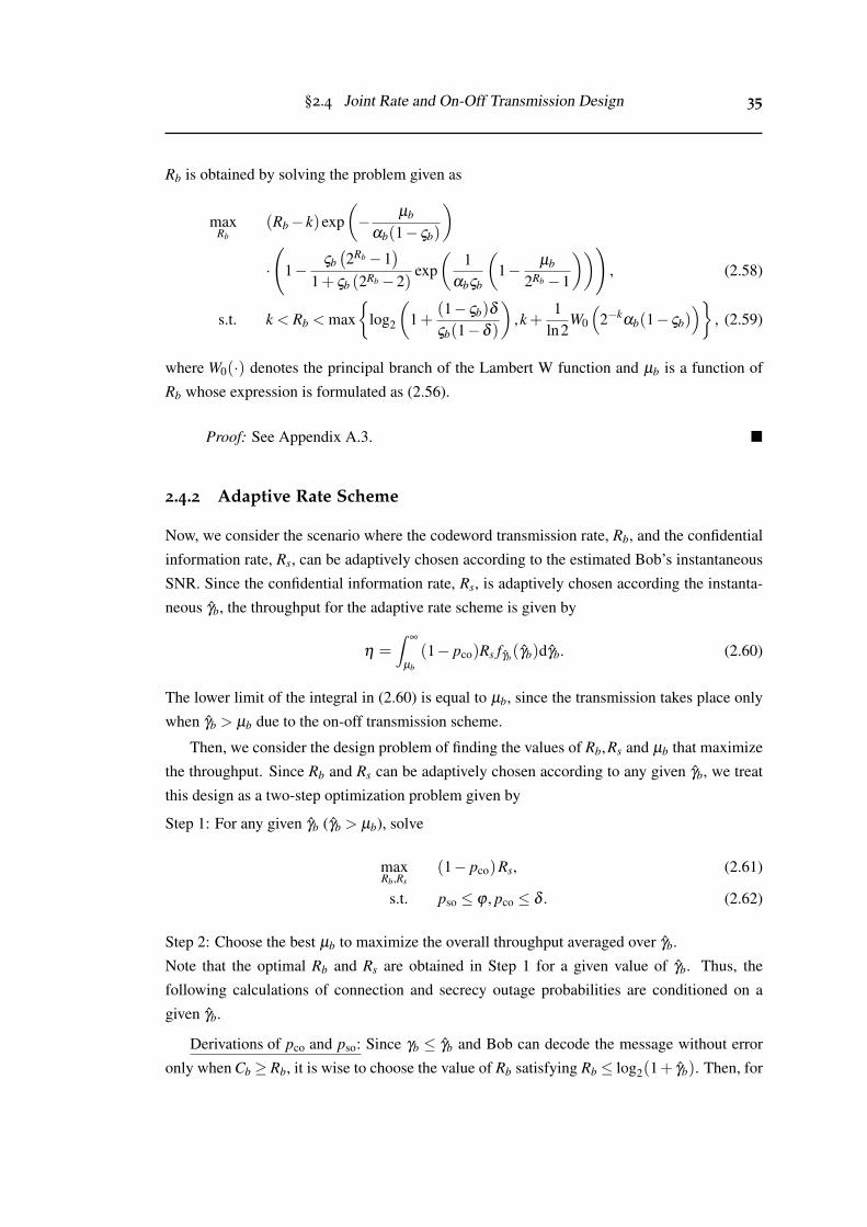
§2.4 Joint Rate and On-Off Transmission Design 35
Rb is obtained by solving the problem given as
maxRb
(Rb− k)exp(− µb
αb(1− ςb)
)·
(1−
ςb(2Rb−1
)1+ ςb (2Rb−2)
exp(
1αbςb
(1− µb
2Rb−1
))), (2.58)
s.t. k < Rb < max{
log2
(1+
(1− ςb)δ
ςb(1−δ )
),k+
1ln2
W0
(2−k
αb(1− ςb))}
, (2.59)
where W0(·) denotes the principal branch of the Lambert W function and µb is a function of
Rb whose expression is formulated as (2.56).
Proof: See Appendix A.3. �
2.4.2 Adaptive Rate Scheme
Now, we consider the scenario where the codeword transmission rate, Rb, and the confidential
information rate, Rs, can be adaptively chosen according to the estimated Bob’s instantaneous
SNR. Since the confidential information rate, Rs, is adaptively chosen according the instanta-
neous γb, the throughput for the adaptive rate scheme is given by
η =∫
∞
µb
(1− pco)Rs fγb(γb)dγb. (2.60)
The lower limit of the integral in (2.60) is equal to µb, since the transmission takes place only
when γb > µb due to the on-off transmission scheme.
Then, we consider the design problem of finding the values of Rb,Rs and µb that maximize
the throughput. Since Rb and Rs can be adaptively chosen according to any given γb, we treat
this design as a two-step optimization problem given by
Step 1: For any given γb (γb > µb), solve
maxRb,Rs
(1− pco)Rs, (2.61)
s.t. pso ≤ ϕ , pco ≤ δ . (2.62)
Step 2: Choose the best µb to maximize the overall throughput averaged over γb.
Note that the optimal Rb and Rs are obtained in Step 1 for a given value of γb. Thus, the
following calculations of connection and secrecy outage probabilities are conditioned on a
given γb.
Derivations of pco and pso: Since γb ≤ γb and Bob can decode the message without error
only when Cb ≥ Rb, it is wise to choose the value of Rb satisfying Rb ≤ log2(1+ γb). Then, for
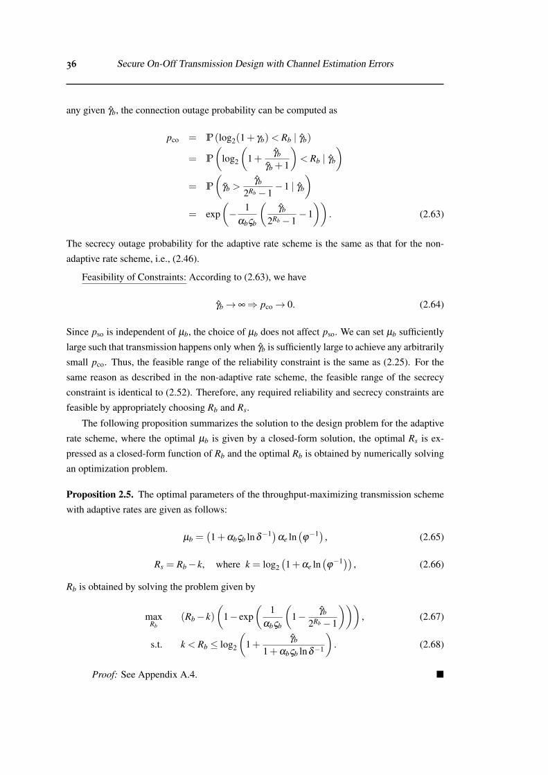
36 Secure On-Off Transmission Design with Channel Estimation Errors
any given γb, the connection outage probability can be computed as
pco = P (log2(1+ γb) < Rb | γb)
= P
(log2
(1+
γb
γb + 1
)< Rb | γb
)= P
(γb >
γb
2Rb−1−1 | γb
)= exp
(− 1
αbςb
(γb
2Rb−1−1))
. (2.63)
The secrecy outage probability for the adaptive rate scheme is the same as that for the non-
adaptive rate scheme, i.e., (2.46).
Feasibility of Constraints: According to (2.63), we have
γb→ ∞⇒ pco→ 0. (2.64)
Since pso is independent of µb, the choice of µb does not affect pso. We can set µb sufficiently
large such that transmission happens only when γb is sufficiently large to achieve any arbitrarily
small pco. Thus, the feasible range of the reliability constraint is the same as (2.25). For the
same reason as described in the non-adaptive rate scheme, the feasible range of the secrecy
constraint is identical to (2.52). Therefore, any required reliability and secrecy constraints are
feasible by appropriately choosing Rb and Rs.
The following proposition summarizes the solution to the design problem for the adaptive
rate scheme, where the optimal µb is given by a closed-form solution, the optimal Rs is ex-
pressed as a closed-form function of Rb and the optimal Rb is obtained by numerically solving
an optimization problem.
Proposition 2.5. The optimal parameters of the throughput-maximizing transmission scheme
with adaptive rates are given as follows:
µb =(1+αbςb lnδ
−1)αe ln
(ϕ−1) , (2.65)
Rs = Rb− k, where k = log2(1+αe ln
(ϕ−1)) , (2.66)
Rb is obtained by solving the problem given by
maxRb
(Rb− k)(
1− exp(
1αbςb
(1− γb
2Rb−1
))), (2.67)
s.t. k < Rb ≤ log2
(1+
γb
1+αbςb lnδ−1
). (2.68)
Proof: See Appendix A.4. �
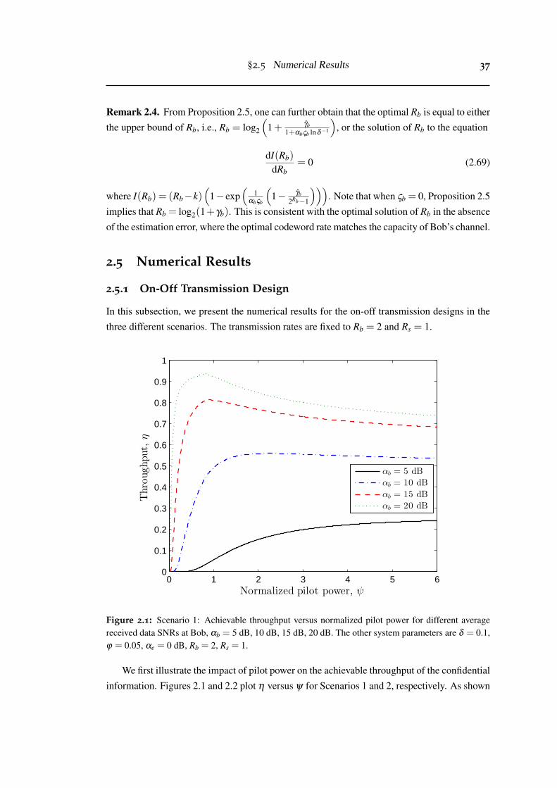
§2.5 Numerical Results 37
Remark 2.4. From Proposition 2.5, one can further obtain that the optimal Rb is equal to either
the upper bound of Rb, i.e., Rb = log2
(1+ γb
1+αbςb lnδ−1
), or the solution of Rb to the equation
dI(Rb)
dRb= 0 (2.69)
where I(Rb) = (Rb−k)(
1− exp(
1αbςb
(1− γb
2Rb−1
))). Note that when ςb = 0, Proposition 2.5
implies that Rb = log2(1+γb). This is consistent with the optimal solution of Rb in the absence
of the estimation error, where the optimal codeword rate matches the capacity of Bob’s channel.
2.5 Numerical Results
2.5.1 On-Off Transmission Design
In this subsection, we present the numerical results for the on-off transmission designs in the
three different scenarios. The transmission rates are fixed to Rb = 2 and Rs = 1.
0 1 2 3 4 5 60
0.1
0.2
0.3
0.4
0.5
0.6
0.7
0.8
0.9
1
Normalized pilot power, ψ
Throughput,
η
αb = 5 dB
αb = 10 dB
αb = 15 dB
αb = 20 dB
Figure 2.1: Scenario 1: Achievable throughput versus normalized pilot power for different averagereceived data SNRs at Bob, αb = 5 dB, 10 dB, 15 dB, 20 dB. The other system parameters are δ = 0.1,ϕ = 0.05, αe = 0 dB, Rb = 2, Rs = 1.
We first illustrate the impact of pilot power on the achievable throughput of the confidential
information. Figures 2.1 and 2.2 plot η versus ψ for Scenarios 1 and 2, respectively. As shown
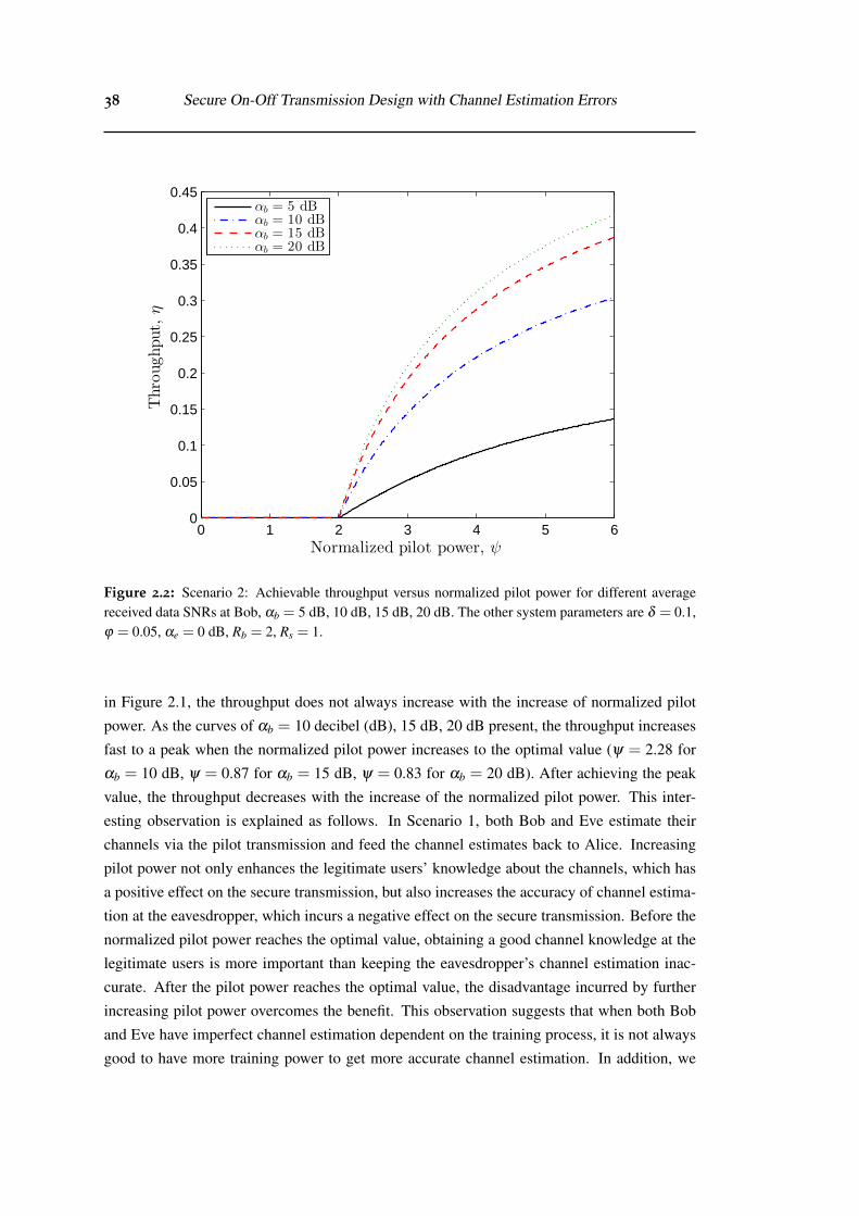
38 Secure On-Off Transmission Design with Channel Estimation Errors
0 1 2 3 4 5 60
0.05
0.1
0.15
0.2
0.25
0.3
0.35
0.4
0.45
Normalized pilot power, ψ
Throughput,
η
αb = 5 dBαb = 10 dBαb = 15 dBαb = 20 dB
Figure 2.2: Scenario 2: Achievable throughput versus normalized pilot power for different averagereceived data SNRs at Bob, αb = 5 dB, 10 dB, 15 dB, 20 dB. The other system parameters are δ = 0.1,ϕ = 0.05, αe = 0 dB, Rb = 2, Rs = 1.
in Figure 2.1, the throughput does not always increase with the increase of normalized pilot
power. As the curves of αb = 10 decibel (dB), 15 dB, 20 dB present, the throughput increases
fast to a peak when the normalized pilot power increases to the optimal value (ψ = 2.28 for
αb = 10 dB, ψ = 0.87 for αb = 15 dB, ψ = 0.83 for αb = 20 dB). After achieving the peak
value, the throughput decreases with the increase of the normalized pilot power. This inter-
esting observation is explained as follows. In Scenario 1, both Bob and Eve estimate their
channels via the pilot transmission and feed the channel estimates back to Alice. Increasing
pilot power not only enhances the legitimate users’ knowledge about the channels, which has
a positive effect on the secure transmission, but also increases the accuracy of channel estima-
tion at the eavesdropper, which incurs a negative effect on the secure transmission. Before the
normalized pilot power reaches the optimal value, obtaining a good channel knowledge at the
legitimate users is more important than keeping the eavesdropper’s channel estimation inac-
curate. After the pilot power reaches the optimal value, the disadvantage incurred by further
increasing pilot power overcomes the benefit. This observation suggests that when both Bob
and Eve have imperfect channel estimation dependent on the training process, it is not always
good to have more training power to get more accurate channel estimation. In addition, we
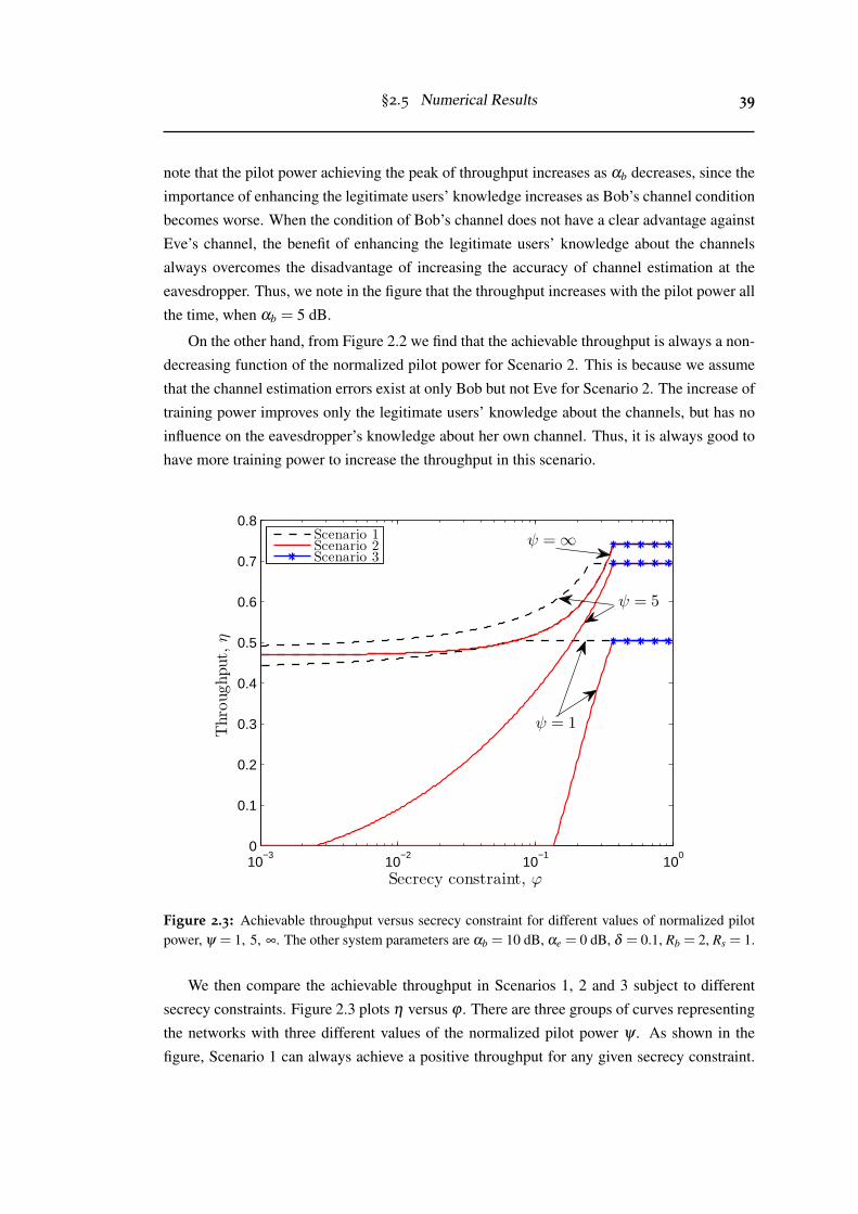
§2.5 Numerical Results 39
note that the pilot power achieving the peak of throughput increases as αb decreases, since the
importance of enhancing the legitimate users’ knowledge increases as Bob’s channel condition
becomes worse. When the condition of Bob’s channel does not have a clear advantage against
Eve’s channel, the benefit of enhancing the legitimate users’ knowledge about the channels
always overcomes the disadvantage of increasing the accuracy of channel estimation at the
eavesdropper. Thus, we note in the figure that the throughput increases with the pilot power all
the time, when αb = 5 dB.
On the other hand, from Figure 2.2 we find that the achievable throughput is always a non-
decreasing function of the normalized pilot power for Scenario 2. This is because we assume
that the channel estimation errors exist at only Bob but not Eve for Scenario 2. The increase of
training power improves only the legitimate users’ knowledge about the channels, but has no
influence on the eavesdropper’s knowledge about her own channel. Thus, it is always good to
have more training power to increase the throughput in this scenario.
10−3
10−2
10−1
100
0
0.1
0.2
0.3
0.4
0.5
0.6
0.7
0.8
ψ = 1
ψ = 5
ψ = ∞
Secrecy constraint, ϕ
Throughput,
η
Scenario 1Scenario 2Scenario 3
Figure 2.3: Achievable throughput versus secrecy constraint for different values of normalized pilotpower, ψ = 1, 5, ∞. The other system parameters are αb = 10 dB, αe = 0 dB, δ = 0.1, Rb = 2, Rs = 1.
We then compare the achievable throughput in Scenarios 1, 2 and 3 subject to different
secrecy constraints. Figure 2.3 plots η versus ϕ . There are three groups of curves representing
the networks with three different values of the normalized pilot power ψ . As shown in the
figure, Scenario 1 can always achieve a positive throughput for any given secrecy constraint.
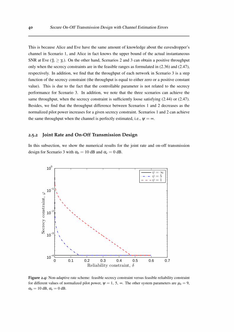
40 Secure On-Off Transmission Design with Channel Estimation Errors
This is because Alice and Eve have the same amount of knowledge about the eavesdropper’s
channel in Scenario 1, and Alice in fact knows the upper bound of the actual instantaneous
SNR at Eve (γe ≥ γe). On the other hand, Scenarios 2 and 3 can obtain a positive throughput
only when the secrecy constraints are in the feasible ranges as formulated in (2.36) and (2.47),
respectively. In addition, we find that the throughput of each network in Scenario 3 is a step
function of the secrecy constraint (the throughput is equal to either zero or a positive constant
value). This is due to the fact that the controllable parameter is not related to the secrecy
performance for Scenario 3. In addition, we note that the three scenarios can achieve the
same throughput, when the secrecy constraint is sufficiently loose satisfying (2.44) or (2.47).
Besides, we find that the throughput difference between Scenarios 1 and 2 decreases as the
normalized pilot power increases for a given secrecy constraint. Scenarios 1 and 2 can achieve
the same throughput when the channel is perfectly estimated, i.e., ψ = ∞.
2.5.2 Joint Rate and On-Off Transmission Design
In this subsection, we show the numerical results for the joint rate and on-off transmission
design for Scenario 3 with αb = 10 dB and αe = 0 dB.
0 0.1 0.2 0.3 0.4 0.5 0.6 0.710
−4
10−3
10−2
10−1
100
Reliability constraint, δ
Secrecyconstraint,
ϕ
ψ = ∞
ψ = 5ψ = 1
Figure 2.4: Non-adaptive rate scheme: feasible secrecy constraint versus feasible reliability constraintfor different values of normalized pilot power, ψ = 1, 5, ∞. The other system parameters are µb = 9,αb = 10 dB, αe = 0 dB.
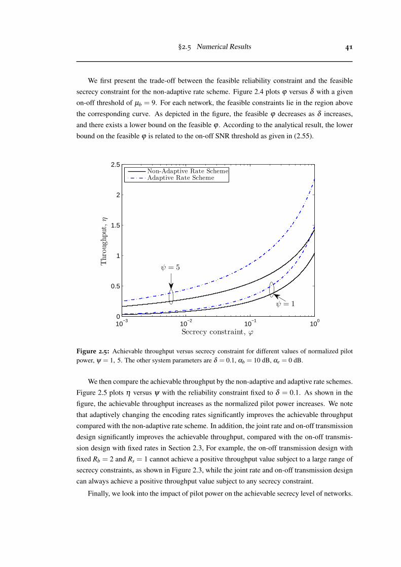
§2.5 Numerical Results 41
We first present the trade-off between the feasible reliability constraint and the feasible
secrecy constraint for the non-adaptive rate scheme. Figure 2.4 plots ϕ versus δ with a given
on-off threshold of µb = 9. For each network, the feasible constraints lie in the region above
the corresponding curve. As depicted in the figure, the feasible ϕ decreases as δ increases,
and there exists a lower bound on the feasible ϕ . According to the analytical result, the lower
bound on the feasible ϕ is related to the on-off SNR threshold as given in (2.55).
10−3
10−2
10−1
100
0
0.5
1
1.5
2
2.5
Secrecy constraint, ϕ
Throughput,
η
ψ = 1
ψ = 5
Non-Adaptive Rate SchemeAdaptive Rate Scheme
Figure 2.5: Achievable throughput versus secrecy constraint for different values of normalized pilotpower, ψ = 1, 5. The other system parameters are δ = 0.1, αb = 10 dB, αe = 0 dB.
We then compare the achievable throughput by the non-adaptive and adaptive rate schemes.
Figure 2.5 plots η versus ψ with the reliability constraint fixed to δ = 0.1. As shown in the
figure, the achievable throughput increases as the normalized pilot power increases. We note
that adaptively changing the encoding rates significantly improves the achievable throughput
compared with the non-adaptive rate scheme. In addition, the joint rate and on-off transmission
design significantly improves the achievable throughput, compared with the on-off transmis-
sion design with fixed rates in Section 2.3, For example, the on-off transmission design with
fixed Rb = 2 and Rs = 1 cannot achieve a positive throughput value subject to a large range of
secrecy constraints, as shown in Figure 2.3, while the joint rate and on-off transmission design
can always achieve a positive throughput value subject to any secrecy constraint.
Finally, we look into the impact of pilot power on the achievable secrecy level of networks.
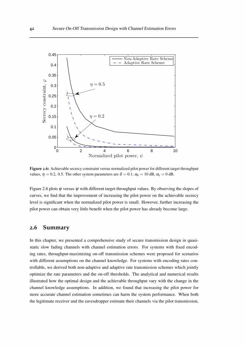
42 Secure On-Off Transmission Design with Channel Estimation Errors
0 2 4 6 8 100
0.05
0.1
0.15
0.2
0.25
0.3
0.35
0.4
0.45
Normalized pilot power, ψ
Secrecyconstraint,
ϕ
η = 0.5
η = 0.2
Non-Adaptive Rate SchemeAdaptive Rate Scheme
Figure 2.6: Achievable secrecy constraint versus normalized pilot power for different target throughputvalues, η = 0.2, 0.5. The other system parameters are δ = 0.1, αb = 10 dB, αe = 0 dB.
Figure 2.6 plots ϕ versus ψ with different target throughput values. By observing the slopes of
curves, we find that the improvement of increasing the pilot power on the achievable secrecy
level is significant when the normalized pilot power is small. However, further increasing the
pilot power can obtain very little benefit when the pilot power has already become large.
2.6 Summary
In this chapter, we presented a comprehensive study of secure transmission design in quasi-
static slow fading channels with channel estimation errors. For systems with fixed encod-
ing rates, throughput-maximizing on-off transmission schemes were proposed for scenarios
with different assumptions on the channel knowledge. For systems with encoding rates con-
trollable, we derived both non-adaptive and adaptive rate transmission schemes which jointly
optimize the rate parameters and the on-off thresholds. The analytical and numerical results
illustrated how the optimal design and the achievable throughput vary with the change in the
channel knowledge assumptions. In addition, we found that increasing the pilot power for
more accurate channel estimation sometimes can harm the system performance. When both
the legitimate receiver and the eavesdropper estimate their channels via the pilot transmission,

§2.6 Summary 43
increasing pilot power decreases the channel estimation errors at both the legitimate receiver
and the eavesdropper. As the pilot power increases, the overall throughput increases at the
beginning but can decrease after achieving the peak value.

44 Secure On-Off Transmission Design with Channel Estimation Errors
Chapter 3
Achieving Secrecy without Knowingthe Number of EavesdropperAntennas
3.1 Introduction
Chapter 2 studied the secure transmission design for single-antenna systems with the practi-
cal assumption of imperfect CSI. In recent years, the fast development of MIMO techniques
has triggered a considerable amount of attention on physical layer security in multi-antenna
systems, where the transmitter, the receiver and/or the eavesdropper are equipped with mul-
tiple antennas. For example, the secrecy capacity of the multi-antenna system was analyzed
in [49, 50, 51] and signal processing techniques with multiple antennas for improving the se-
crecy performance were proposed in [27, 28, 37, 52, 53]. Apart from the assumption of perfect
CSI, current research on physical layer security in multi-antenna systems is often based on
another idealized assumption, i.e., knowing the number of eavesdropper antennas or setting an
upper bound on the number of eavesdropper antennas. Knowing the number of eavesdropper
antennas is impractical in most of actual systems, since an external eavesdropper naturally does
not inform the legitimate side about the number of antennas to expose its ability. Estimating
an upper bound on the number of antennas according the device size is also almost impossible,
since the current development of large-scale antenna array technologies allows a fast growing
number of antennas to place within a limited space.
In this chapter, we provide an innovative solution to the important problem of how to char-
acterize the performance of physical layer security without knowing the number of eavesdrop-
per antennas problem. To this end, we introduce the concept of spatial constraint into physical
layer security. We focus on the effects of spatial constraints at the receiver side. Specifically,
we consider the scenario where the transmitter has a large number of antennas without spatial
constraint while both the intended receiver and the eavesdropper have spatial constraints to
place the receive antennas. This is a valid assumption given less geometrical size restriction
45
46 Achieving Secrecy without Knowing the Number of Eavesdropper Antennas
for the BS to place a large number of transmit antennas, while the size of receiving device in
the downlink is often relatively small [70]. Importantly, the number of receive antennas at the
eavesdropper may not be known. We consider a simple and practical CSI assumption that the
instantaneous CSI is known at the receiver end (the intended receiver and the eavesdropper)
but not at the transmitter. Under these assumptions and considerations, we derive the secrecy
capacity of the spatially-constrained multi-antenna system, and study the potential benefits
brought by two widely-adopted friendly-jamming techniques. The two friendly-jamming tech-
niques studied are the basic jamming technique and the AN jamming technique: the former
degrades both the intended receiver and the eavesdropper’s channels, while the latter degrades
only the eavesdropper’s channel but does not affect the intended receiver’s channel. We find
that a non-zero secrecy capacity is achievable for the spatially-constrained system with the
help of friendly-jamming signals, even if the number of eavesdropper antennas is unknown
and considered to be infinity as a worst case.
The remainder of this chapter is organized as follows. Section 3.2 describes system models
for studying physical layer security with spatial constraints at the receiver side. In Section 3.3,
we first give the secrecy capacity of the proposed systems with the knowledge of the number
of eavesdropper antennas. The important case of not knowing the number of eavesdropper
antennas is studied in Section 3.4, where the eavesdropper’s receiver is assumed to be noise
free and allowed to have infinitely many antennas for the worst-case consideration. Finally,
Section 3.5 summarizes the chapter.
3.2 System Model
In this chapter, we study physical layer security in multi-antenna systems with spatial con-
straints at the receiver side. We assume that all communication nodes are equipped with multi-
ple antennas and there exist spatial constraints at both the intended receiver and the eavesdrop-
per. That is, the intended receiver and the eavesdropper have limited sizes of spatial regions
for placing the receive antennas. To focus on the impact of spatial constraints at the receiver
side, we adopt the following two assumptions as briefly mentioned in Section 3.1. Firstly,
we assume that there is no spatial constraint at the transmitter side for placing transmit anten-
nas. Secondly, we assume that the transmitter has a large number of transmit antennas, and
hence the capacity of the channel from the transmitter to the receiver is mainly restricted by
the receiver side. Note that the number of antennas at the BS is often predicted to be in the
hundreds for the next generation wireless systems [71, 72]. These two assumptions were of-
ten adopted in the literature investigating the impact of spatial constraints at the receiver side
on multi-antenna systems without secrecy considerations, e.g., [70, 73, 74, 75] studying the
channel capacity and [76, 77, 78, 79] studying the spatial degrees of freedom. We specifically
investigate two different secure communication systems, which are the wiretap-channel sys-
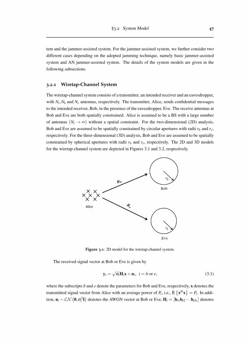
§3.2 System Model 47
tem and the jammer-assisted system. For the jammer-assisted system, we further consider two
different cases depending on the adopted jamming technique, namely basic jammer-assisted
system and AN jammer-assisted system. The details of the system models are given in the
following subsections.
3.2.1 Wiretap-Channel System
The wiretap-channel system consists of a transmitter, an intended receiver and an eavesdropper,
with Nt ,Nb and Ne antennas, respectively. The transmitter, Alice, sends confidential messages
to the intended receiver, Bob, in the presence of the eavesdropper, Eve. The receive antennas at
Bob and Eve are both spatially constrained. Alice is assumed to be a BS with a large number
of antennas (Nt → ∞) without a spatial constraint. For the two-dimensional (2D) analysis,
Bob and Eve are assumed to be spatially constrained by circular apertures with radii rb and re,
respectively. For the three-dimensional (3D) analysis, Bob and Eve are assumed to be spatially
constrained by spherical apertures with radii rb and re, respectively. The 2D and 3D models
for the wiretap-channel system are depicted in Figures 3.1 and 3.2, respectively.
Figure 3.1: 2D model for the wiretap-channel system.
The received signal vector at Bob or Eve is given by
yi =√
αiHix+ni, i = b or e, (3.1)
where the subscripts b and e denote the parameters for Bob and Eve, respectively, x denotes the
transmitted signal vector from Alice with an average power of Pt , i.e., E{
xHx}= Pt . In addi-
tion, ni ∼ CN(0,σ2
i I)
denotes the AWGN vector at Bob or Eve, Hi = [hi1hi2 · · ·hiNt ] denotes
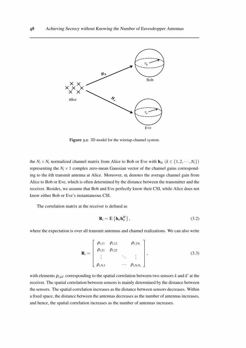
48 Achieving Secrecy without Knowing the Number of Eavesdropper Antennas
Figure 3.2: 3D model for the wiretap-channel system.
the Ni×Nt normalized channel matrix from Alice to Bob or Eve with hik (k ∈ {1,2, · · · ,Nt})representing the Ni×1 complex zero-mean Gaussian vector of the channel gains correspond-
ing to the kth transmit antenna at Alice. Moreover, αi denotes the average channel gain from
Alice to Bob or Eve, which is often determined by the distance between the transmitter and the
receiver. Besides, we assume that Bob and Eve perfectly know their CSI, while Alice does not
know either Bob or Eve’s instantaneous CSI.
The correlation matrix at the receiver is defined as
Ri = E{
hithHit}
, (3.2)
where the expectation is over all transmit antennas and channel realizations. We can also write
Ri =
ρi,11 ρi,12 ρi,1Ni
ρi,21 ρi,22...
. . ....
ρi,Ni1 · · · ρi,NiNi
, (3.3)
with elements ρi,kk′ corresponding to the spatial correlation between two sensors k and k′ at the
receiver. The spatial correlation between sensors is mainly determined by the distance between
the sensors. The spatial correlation increases as the distance between sensors decreases. Within
a fixed space, the distance between the antennas decreases as the number of antennas increases,
and hence, the spatial correlation increases as the number of antennas increases.
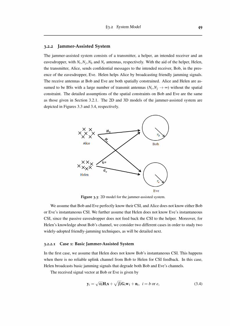
§3.2 System Model 49
3.2.2 Jammer-Assisted System
The jammer-assisted system consists of a transmitter, a helper, an intended receiver and an
eavesdropper, with Nt ,N j,Nb and Ne antennas, respectively. With the aid of the helper, Helen,
the transmitter, Alice, sends confidential messages to the intended receiver, Bob, in the pres-
ence of the eavesdropper, Eve. Helen helps Alice by broadcasting friendly jamming signals.
The receive antennas at Bob and Eve are both spatially constrained. Alice and Helen are as-
sumed to be BSs with a large number of transmit antennas (Nt ,N j → ∞) without the spatial
constraint. The detailed assumptions of the spatial constraints on Bob and Eve are the same
as those given in Section 3.2.1. The 2D and 3D models of the jammer-assisted system are
depicted in Figures 3.3 and 3.4, respectively.
Figure 3.3: 2D model for the jammer-assisted system.
We assume that Bob and Eve perfectly know their CSI, and Alice does not know either Bob
or Eve’s instantaneous CSI. We further assume that Helen does not know Eve’s instantaneous
CSI, since the passive eavesdropper does not feed back the CSI to the helper. Moreover, for
Helen’s knowledge about Bob’s channel, we consider two different cases in order to study two
widely-adopted friendly-jamming techniques, as will be detailed next.
3.2.2.1 Case 1: Basic Jammer-Assisted System
In the first case, we assume that Helen does not know Bob’s instantaneous CSI. This happens
when there is no reliable uplink channel from Bob to Helen for CSI feedback. In this case,
Helen broadcasts basic jamming signals that degrade both Bob and Eve’s channels.
The received signal vector at Bob or Eve is given by
yi =√
αiHix+√
βiGiw1 +ni, i = b or e, (3.4)
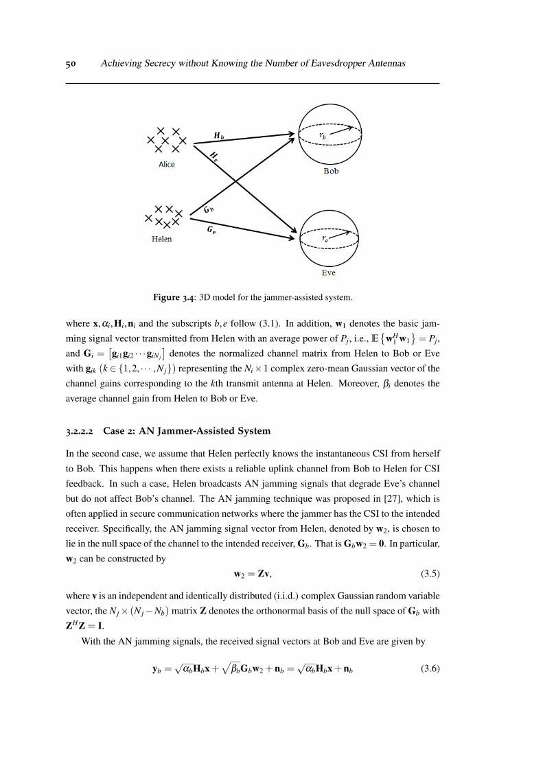
50 Achieving Secrecy without Knowing the Number of Eavesdropper Antennas
Figure 3.4: 3D model for the jammer-assisted system.
where x,αi,Hi,ni and the subscripts b,e follow (3.1). In addition, w1 denotes the basic jam-
ming signal vector transmitted from Helen with an average power of Pj, i.e., E{
wH1 w1
}= Pj,
and Gi =[gi1gi2 · · ·giN j
]denotes the normalized channel matrix from Helen to Bob or Eve
with gik (k ∈ {1,2, · · · ,N j}) representing the Ni×1 complex zero-mean Gaussian vector of the
channel gains corresponding to the kth transmit antenna at Helen. Moreover, βi denotes the
average channel gain from Helen to Bob or Eve.
3.2.2.2 Case 2: AN Jammer-Assisted System
In the second case, we assume that Helen perfectly knows the instantaneous CSI from herself
to Bob. This happens when there exists a reliable uplink channel from Bob to Helen for CSI
feedback. In such a case, Helen broadcasts AN jamming signals that degrade Eve’s channel
but do not affect Bob’s channel. The AN jamming technique was proposed in [27], which is
often applied in secure communication networks where the jammer has the CSI to the intended
receiver. Specifically, the AN jamming signal vector from Helen, denoted by w2, is chosen to
lie in the null space of the channel to the intended receiver, Gb. That is Gbw2 = 0. In particular,
w2 can be constructed by
w2 = Zv, (3.5)
where v is an independent and identically distributed (i.i.d.) complex Gaussian random variable
vector, the N j× (N j−Nb) matrix Z denotes the orthonormal basis of the null space of Gb with
ZHZ = I.
With the AN jamming signals, the received signal vectors at Bob and Eve are given by
yb =√
αbHbx+√
βbGbw2 +nb =√
αbHbx+nb (3.6)
§3.3 Introducing Spatial Constraints into Secrecy Capacity Calculation 51
and
ye =√
αeHex+√
βeGew2 +ne =√
αeHex+√
βeGeZv+ne, (3.7)
respectively, where, once again, x,αb,αe,Hb,He,nb,ne follow (3.1) and βb,βe,Gb,Ge fol-
low (3.4). Besides, the average transmit power at Helen is still given by Pj, i.e., E{
wH2 w2
}=
Pj.
Remark 3.1. We highlight that the analysis for the AN jammer-assisted system is mainly mo-
tivated by its importance from the theoretical point of view. The basic jamming and the AN
jamming are the two most widely-studied physical-layer techniques to improve the secrecy
performance of multi-antenna systems. In this chapter, we study the wireless physical layer se-
curity with spatial constraints at the receiver side. It is of significant importance to investigate
the benefits brought by both of the jamming techniques in the spatially-constrained systems.
The AN jamming technique is often studied in the scenario where both Alice and Helen have
the legitimate CSI in the literature. The legitimate CSI available at Alice enables not only the
injection of AN jamming signals but also the transmit beamforming, and the secrecy capacity
will go to infinity under the assumption of infinitely large number of transmit antennas. This
will be shown later in Section 3.3. In order to investigate the capacity improvement solely
brought by AN jamming, we assume that Alice does not know the instantaneous CSI to Bob,
but Helen knows the instantaneous CSI to Bob. Besides, the practical value of the AN jammer-
assisted system studied in this chapter can be seen from the following scenario as an example:
We can consider that Alice is a BS owned by company A to serve a mobile user, Bob. Helen
is another BS owned by company B. Due to particular reasons, e.g., location or surrounding
environment, the CSI feedback link from Bob to Alice is bad, while the CSI feedback link
from Bob to Helen is good. Then, Alice asks Helen to help the secrecy transmission by broad-
casting AN jamming signals. For the secrecy concern, company A does not intend to share
the confidential information with company B, and hence Alice does not share the messages to
transmit with Helen.
3.3 Introducing Spatial Constraints into Secrecy Capacity Cal-culation
In this section, we derive the secrecy capacity of the systems with spatial constraints at the
receiver side as described in Section 3.2. The secrecy capacity characterizes the maximum rate
at which messages can be reliably transmitted to Bob while Eve obtains zero information. It is
mathematically defined by [15]
Cs = [Cb−Ce]+, (3.8)
where Cb and Ce denote Bob and Eve’s channel capacities, respectively.
52 Achieving Secrecy without Knowing the Number of Eavesdropper Antennas
For the multi-antenna systems with spatial constraint at the receiver, the channel capacity is
limited by the rank and the eigenvalues of the spatial correlation matrix at the receiver. As the
number of antennas increases in a fixed space, the correlation between antennas increases. The
increase in spatial correlation will limit the number of significant eigenvalues of the spatial cor-
relation matrix. As more antennas are placed in the fixed space, they will be highly correlated
with other antennas. As a result, the growth of channel capacity with respect to the number
of receive antennas reduces from linear to logarithmic. The number of receive antennas at
which the capacity scaling is reduced to logarithmic is approximated by the saturation number
of receive antennas. The saturation number of receive antennas is given by [70, Chapters 3.3]
N0i =
{2dπeri/λe+ 1 , for 2D analysis
(dπeri/λe+ 1)2 , for 3D analysis,(3.9)
where λ denotes the wavelength, e denotes Euler’s number, and subscript i denotes the param-
eters for Bob or Eve. As pointed out in [70], the growth of channel capacity (Cb or Ce) with
respect to the number of optimally-placed receive antennas (Nb or Ne) reduces from linear to
logarithmic when the number of receive antennas increases beyond the saturation number (N0b
or N0e). Note that similar “saturation" effects on the growth of channel capacity with respect
to the number of antennas at the spatially-constrained receiver have also been pointed out in,
e.g., [80, 81, 82, 83].
It is worth mentioning that the capacity results in this chapter are approximations based on
(3.9) and the assumption of infinitely large number of transmit antennas. The accuracy of the
approximations are verified in Appendices. In the rest of the chapter, we simply refer to the
approximated capacity result as the capacity.
3.3.1 Secrecy Capacity of Wiretap-Channel System
Proposition 3.1. The secrecy capacity of the wiretap-channel system with spatial constraints
at the receiver side is given by Cs = [Cb−Ce]+ where
Cb =
Nb log2(1+αbPtσ2
b) , if Nb ≤ N0b
N0b log2(1+NbN0b
αbPtσ2
b) , if Nb > N0b,
(3.10)
Ce =
{Ne log2(1+
αePtσ2
e) , if Ne ≤ N0e
N0e log2(1+NeN0e
αePtσ2
e) , if Ne > N0e.
(3.11)
Proof: The capacities of the channels to the spatially-constrained Bob and Eve follow
easily from [70, Chapters 2 and 3]. The details are given in Appendix B.1. �
Proposition 3.1 gives the secrecy capacity of the wiretap-channel system taking spatial
constraints at the receiver side into account. From Proposition 3.1, we note that the growth of
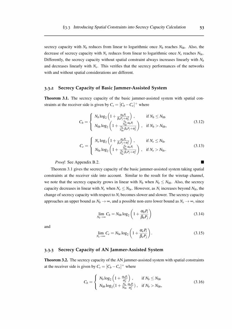
§3.3 Introducing Spatial Constraints into Secrecy Capacity Calculation 53
secrecy capacity with Nb reduces from linear to logarithmic once Nb reaches N0b. Also, the
decrease of secrecy capacity with Ne reduces from linear to logarithmic once Ne reaches N0e.
Differently, the secrecy capacity without spatial constraint always increases linearly with Nb
and decreases linearly with Ne. This verifies that the secrecy performances of the networks
with and without spatial considerations are different.
3.3.2 Secrecy Capacity of Basic Jammer-Assisted System
Theorem 3.1. The secrecy capacity of the basic jammer-assisted system with spatial con-
straints at the receiver side is given by Cs = [Cb−Ce]+ where
Cb =
Nb log2
(1+ αbPt
βbPj+σ2b
), if Nb ≤ N0b
N0b log2
(1+
NbN0b
αbPtNbN0b
βbPj+σ2b
), if Nb > N0b,
(3.12)
Ce =
Ne log2
(1+ αePt
βePj+σ2e
), if Ne ≤ N0e
N0e log2
(1+
NeN0e
αePtNeN0e
βePj+σ2e
), if Ne > N0e.
(3.13)
Proof: See Appendix B.2. �
Theorem 3.1 gives the secrecy capacity of the basic jammer-assisted system taking spatial
constraints at the receiver side into account. Similar to the result for the wiretap channel,
we note that the secrecy capacity grows in linear with Nb when Nb ≤ N0b. Also, the secrecy
capacity decreases in linear with Ne when Ne ≤ N0e. However, as Ni increases beyond N0i, the
change of secrecy capacity with respect to Ni becomes slower and slower. The secrecy capacity
approaches an upper bound as Nb→∞, and a possible non-zero lower bound as Ne→∞, since
limNb→∞
Cb = N0b log2
(1+
αbPt
βbPj
)(3.14)
and
limNe→∞
Ce = N0e log2
(1+
αePt
βePj
). (3.15)
3.3.3 Secrecy Capacity of AN Jammer-Assisted System
Theorem 3.2. The secrecy capacity of the AN jammer-assisted system with spatial constraints
at the receiver side is given by Cs = [Cb−Ce]+ where
Cb =
Nb log2
(1+ αbPt
σ2b
), if Nb ≤ N0b
N0b log2(1+NbN0b
αbPtσ2
b) , if Nb > N0b,
(3.16)
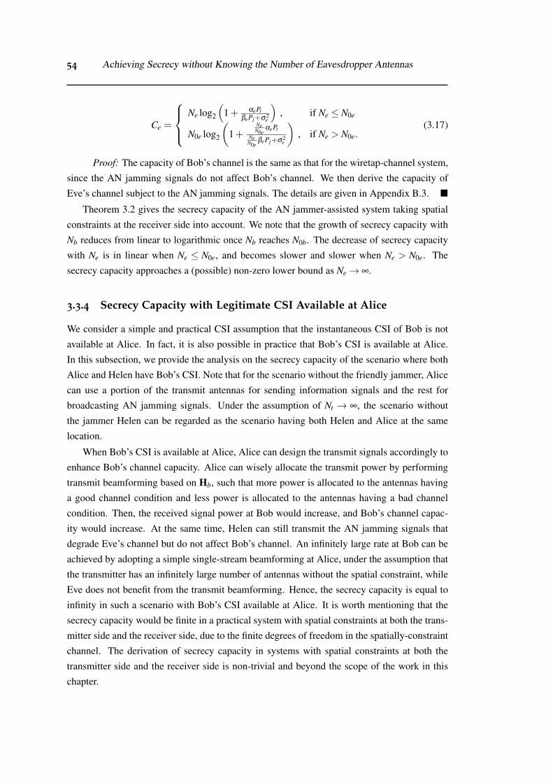
54 Achieving Secrecy without Knowing the Number of Eavesdropper Antennas
Ce =
Ne log2
(1+ αePt
βePj+σ2e
), if Ne ≤ N0e
N0e log2
(1+
NeN0e
αePtNeN0e
βePj+σ2e
), if Ne > N0e.
(3.17)
Proof: The capacity of Bob’s channel is the same as that for the wiretap-channel system,
since the AN jamming signals do not affect Bob’s channel. We then derive the capacity of
Eve’s channel subject to the AN jamming signals. The details are given in Appendix B.3. �
Theorem 3.2 gives the secrecy capacity of the AN jammer-assisted system taking spatial
constraints at the receiver side into account. We note that the growth of secrecy capacity with
Nb reduces from linear to logarithmic once Nb reaches N0b. The decrease of secrecy capacity
with Ne is in linear when Ne ≤ N0e, and becomes slower and slower when Ne > N0e. The
secrecy capacity approaches a (possible) non-zero lower bound as Ne→ ∞.
3.3.4 Secrecy Capacity with Legitimate CSI Available at Alice
We consider a simple and practical CSI assumption that the instantaneous CSI of Bob is not
available at Alice. In fact, it is also possible in practice that Bob’s CSI is available at Alice.
In this subsection, we provide the analysis on the secrecy capacity of the scenario where both
Alice and Helen have Bob’s CSI. Note that for the scenario without the friendly jammer, Alice
can use a portion of the transmit antennas for sending information signals and the rest for
broadcasting AN jamming signals. Under the assumption of Nt → ∞, the scenario without
the jammer Helen can be regarded as the scenario having both Helen and Alice at the same
location.
When Bob’s CSI is available at Alice, Alice can design the transmit signals accordingly to
enhance Bob’s channel capacity. Alice can wisely allocate the transmit power by performing
transmit beamforming based on Hb, such that more power is allocated to the antennas having
a good channel condition and less power is allocated to the antennas having a bad channel
condition. Then, the received signal power at Bob would increase, and Bob’s channel capac-
ity would increase. At the same time, Helen can still transmit the AN jamming signals that
degrade Eve’s channel but do not affect Bob’s channel. An infinitely large rate at Bob can be
achieved by adopting a simple single-stream beamforming at Alice, under the assumption that
the transmitter has an infinitely large number of antennas without the spatial constraint, while
Eve does not benefit from the transmit beamforming. Hence, the secrecy capacity is equal to
infinity in such a scenario with Bob’s CSI available at Alice. It is worth mentioning that the
secrecy capacity would be finite in a practical system with spatial constraints at both the trans-
mitter side and the receiver side, due to the finite degrees of freedom in the spatially-constraint
channel. The derivation of secrecy capacity in systems with spatial constraints at both the
transmitter side and the receiver side is non-trivial and beyond the scope of the work in this
chapter.
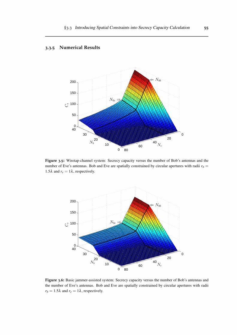
§3.3 Introducing Spatial Constraints into Secrecy Capacity Calculation 55
3.3.5 Numerical Results
020
4060
800
10
20
30
400
50
100
150
200⇐ N0b
Ne
N0e ⇒
Nb
Cs
Figure 3.5: Wiretap-channel system: Secrecy capacity versus the number of Bob’s antennas and thenumber of Eve’s antennas. Bob and Eve are spatially constrained by circular apertures with radii rb =
1.5λ and re = 1λ , respectively.
020
4060
800
10
20
30
400
50
100
150
200⇐ N0b
Ne
N0e ⇒
Nb
Cs
Figure 3.6: Basic jammer-assisted system: Secrecy capacity versus the number of Bob’s antennas andthe number of Eve’s antennas. Bob and Eve are spatially constrained by circular apertures with radiirb = 1.5λ and re = 1λ , respectively.
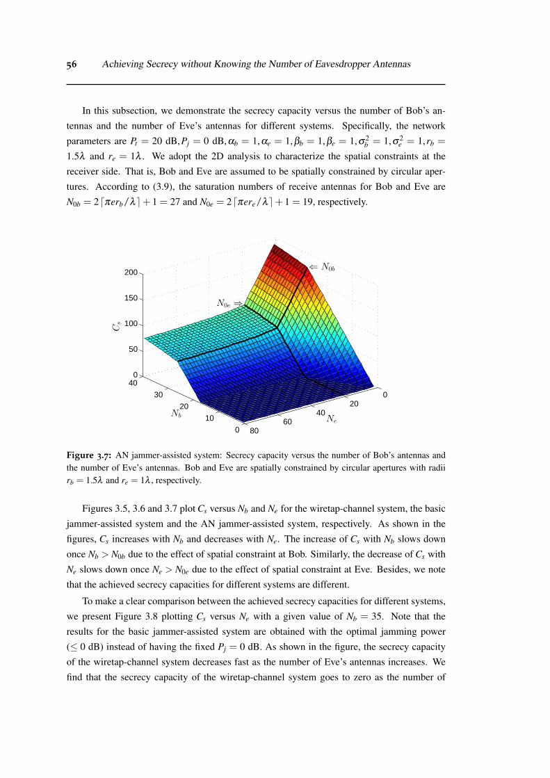
56 Achieving Secrecy without Knowing the Number of Eavesdropper Antennas
In this subsection, we demonstrate the secrecy capacity versus the number of Bob’s an-
tennas and the number of Eve’s antennas for different systems. Specifically, the network
parameters are Pt = 20 dB,Pj = 0 dB,αb = 1,αe = 1,βb = 1,βe = 1,σ2b = 1,σ2
e = 1,rb =
1.5λ and re = 1λ . We adopt the 2D analysis to characterize the spatial constraints at the
receiver side. That is, Bob and Eve are assumed to be spatially constrained by circular aper-
tures. According to (3.9), the saturation numbers of receive antennas for Bob and Eve are
N0b = 2dπerb/λe+ 1 = 27 and N0e = 2dπere/λe+ 1 = 19, respectively.
020
4060
800
10
20
30
400
50
100
150
200⇐ N0b
Ne
N0e ⇒
Nb
Cs
Figure 3.7: AN jammer-assisted system: Secrecy capacity versus the number of Bob’s antennas andthe number of Eve’s antennas. Bob and Eve are spatially constrained by circular apertures with radiirb = 1.5λ and re = 1λ , respectively.
Figures 3.5, 3.6 and 3.7 plot Cs versus Nb and Ne for the wiretap-channel system, the basic
jammer-assisted system and the AN jammer-assisted system, respectively. As shown in the
figures, Cs increases with Nb and decreases with Ne. The increase of Cs with Nb slows down
once Nb > N0b due to the effect of spatial constraint at Bob. Similarly, the decrease of Cs with
Ne slows down once Ne > N0e due to the effect of spatial constraint at Eve. Besides, we note
that the achieved secrecy capacities for different systems are different.
To make a clear comparison between the achieved secrecy capacities for different systems,
we present Figure 3.8 plotting Cs versus Ne with a given value of Nb = 35. Note that the
results for the basic jammer-assisted system are obtained with the optimal jamming power
(≤ 0 dB) instead of having the fixed Pj = 0 dB. As shown in the figure, the secrecy capacity
of the wiretap-channel system decreases fast as the number of Eve’s antennas increases. We
find that the secrecy capacity of the wiretap-channel system goes to zero as the number of
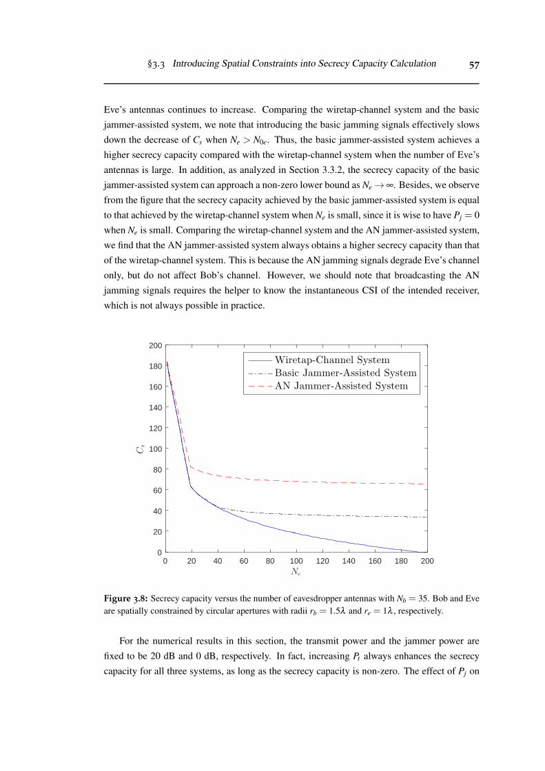
§3.3 Introducing Spatial Constraints into Secrecy Capacity Calculation 57
Eve’s antennas continues to increase. Comparing the wiretap-channel system and the basic
jammer-assisted system, we note that introducing the basic jamming signals effectively slows
down the decrease of Cs when Ne > N0e. Thus, the basic jammer-assisted system achieves a
higher secrecy capacity compared with the wiretap-channel system when the number of Eve’s
antennas is large. In addition, as analyzed in Section 3.3.2, the secrecy capacity of the basic
jammer-assisted system can approach a non-zero lower bound as Ne→∞. Besides, we observe
from the figure that the secrecy capacity achieved by the basic jammer-assisted system is equal
to that achieved by the wiretap-channel system when Ne is small, since it is wise to have Pj = 0
when Ne is small. Comparing the wiretap-channel system and the AN jammer-assisted system,
we find that the AN jammer-assisted system always obtains a higher secrecy capacity than that
of the wiretap-channel system. This is because the AN jamming signals degrade Eve’s channel
only, but do not affect Bob’s channel. However, we should note that broadcasting the AN
jamming signals requires the helper to know the instantaneous CSI of the intended receiver,
which is not always possible in practice.
0 20 40 60 80 100 120 140 160 180 2000
20
40
60
80
100
120
140
160
180
200
Ne
Cs
Wiretap-Channel System
Basic Jammer-Assisted System
AN Jammer-Assisted System
Figure 3.8: Secrecy capacity versus the number of eavesdropper antennas with Nb = 35. Bob and Eveare spatially constrained by circular apertures with radii rb = 1.5λ and re = 1λ , respectively.
For the numerical results in this section, the transmit power and the jammer power are
fixed to be 20 dB and 0 dB, respectively. In fact, increasing Pt always enhances the secrecy
capacity for all three systems, as long as the secrecy capacity is non-zero. The effect of Pj on
58 Achieving Secrecy without Knowing the Number of Eavesdropper Antennas
the secrecy capacity is complicated and will be detailed in Section 3.4.
3.4 Worst-Case Analysis for Jammer-Assisted Systems
The previous section provides the basic analysis on the secure communication systems with
spatial constraints at the receiver side. However, to evaluate the system performance by the ca-
pacity results given in Proposition 3.1, Theorems 3.1 and 3.2, we require very good knowledge
on Eve, including Ne and σ2e . In practice, it is desirable to be able to investigate the secrecy
performance of a system without the knowledge of Ne and σ2e . To this end, we consider a
“worst-case eavesdropper" (from the legitimate users’ perspective) as in this section.
For such a worst-case eavesdropper, we assume that the number of receive antennas at the
eavesdropper approaches infinity and the noise variance at the eavesdropper approaches zero,
i.e, Ne→∞ and σ2e → 0. Then, the secrecy capacity with the worst-case consideration is given
by
Cws = lim
Ne→∞,σ2e→0
Cs, (3.18)
where Cs is the secrecy capacity of systems with perfect knowledge of Ne and σ2e , i.e, the
secrecy capacity derived in the previous section. In addition, we refer to Cws as the worst-case
secrecy capacity.
The worst-case scenario is motivated by the fact that the eavesdropper’s ability is difficult
to be known or controlled by the legitimate side. As such, in the design of secure communica-
tions, we assume the worst-case scenario where the eavesdropper can deploy infinite number
of antennas with arbitrarily small noise variance. If we assume that the eavesdropper has a
given number of antennas, the designed secure communications would be vulnerable to eaves-
dropping caused by a larger number of antennas at the eavesdropper in practice. Therefore, the
weaker assumption of knowing a finite number of antennas at the eavesdropper cannot lead to
the true guarantee of security, and thus it is of critical significance to take into consideration
the worst-case scenario with infinite number of eavesdropper antennas.
3.4.1 Wiretap-Channel System
Based on Proposition 3.1 and (3.18), the worst-case secrecy capacity of the wiretap-channel
system is given by
Cws = 0. (3.19)
We note that a non-zero worst-case secrecy capacity is not achievable under any condition for
the wiretap-channel system, because the capacity of Eve’s channel always goes to infinity with
Ne→ ∞ or σ2e → 0.
§3.4 Worst-Case Analysis for Jammer-Assisted Systems 59
3.4.2 Basic Jammer-Assisted System
3.4.2.1 Worst-Case Secrecy Capacity
Based on Theorem 3.1 and (3.18), the worst-case secrecy capacity of the basic jammer-assisted
system is given by
Cws =
[Nb log2
(1+ αbPt
βbPj+σ2b
)−N0e log2
(1+ αePt
βePj
)]+, if Nb ≤ N0b[
N0b log2
(1+
NbN0b
αbPtNbN0b
βbPj+σ2b
)−N0e log2
(1+ αePt
βePj
)]+, if Nb > N0b.
(3.20)
From (3.20), we note that a non-zero worst-case secrecy capacity sometimes is achievable
for the basic jammer-assisted system depending on the system parameters, such as transmit
power, average channel gains, the spatial constraint at Bob and the number of antennas at
Bob. This result shows for the first time that a non-zero secrecy rate can be achieved even if
the eavesdropper’s receiver itself is noise free and allowed to have infinitely many antennas.
Moreover, this is achieved by simply asking a friendly-jamming node to send random jamming
signals.
To further study the condition for having a non-zero worst-case secrecy capacity, we con-
sider the scenario where the number of antennas at Bob, Nb, is controllable and the other system
parameters1, i.e., N0b,N0e,αb,βb,αe,βe,Pt and Pj, are fixed. From (3.20), we find that a non-
zero worst-case secrecy capacity is always achievable by having “enough" receive antennas at
Bob when N0b log2
(1+ αbPt
βbPj
)> N0e log2
(1+ αePt
βePj
). However, the secrecy capacity is always
equal to zero when
N0b log2
(1+
αbPt
βbPj
)≤ N0e log2
(1+
αePt
βePj
), (3.21)
because Cb < N0b log2
(1+ αbPt
βbPj
)always holds for any finite value of Nb. In addition, when
N0b log2
(1+ αbPt
βbPj
)> N0e log2
(1+ αePt
βePj
), we can further derive the minimum Nb to ensure a
non-zero worst-case secrecy capacity as
Nb,min =
N0e log2
(1+ αePt
βePj
)log2
(1+ αbPt
βbPj+σ2b
)+ 1 , if N0b log2
(1+ αbPt
βbPj+σ2b
)≥ N0e log2
(1+ αePt
βePj
) N0b œb
2
((1+ ffePt
fiePj
) N0eN0b −1
)
ffbPt+fibPj−fibPj
(1+ ffePt
fiePj
) N0eN0b
+ 1 , otherwise.
(3.22)
1Here the other system parameters depend on the spatial constraint, the location of communication node andthe transmit power.

60 Achieving Secrecy without Knowing the Number of Eavesdropper Antennas
3.4.2.2 Optimal Jamming Power
From (3.20), we note that the worst-case secrecy capacity is not a monotonically increasing
function of the jamming power. This is because the increase of Pj degrades not only Eve’s
channel but also Bob’s channel, and there arises a tradeoff between maintaining the capac-
ity of Bob’s channel and decreasing the capacity of Eve’s channel. In the following, we
determine the optimal jamming power that maximizes the worst-case secrecy capacity, i.e.,
P∗j = argmaxPj Cws .
Proposition 3.2. The optimal jamming power that maximizes the worst-case secrecy capacity
of the basic jammer-assisted system is given by
P∗j =
x1 , if Nb ≤ N0b and f1(x1) > 0 with x1 is real and positive
x2 , if Nb ≤ N0b and f1(x2) > 0 with x2 is real and positive
x3 , if Nb > N0b and f2(x3) > 0 with x3 is real and positive
x4 , if Nb > N0b and f2(x4) > 0 with x4 is real and positive
not applicable, otherwise,
(3.23)
where
f1(x) = Nb log2
(1+
αbPt
βbx+σ2b
)−N0e log2
(1+
αePt
βex
),
f2(x) = N0b log2
(1+
NbN0b
αbPtNbN0b
βbx+σ2b
)−N0e log2
(1+
αePt
βex
),
x1 =2N0eαeσ2
b −Ptαbαe (Nb−N0e)
2 (Nbαbβe−N0eαeβb)
+
√α2
b α2e β 2
b P2t (Nb−N0e)
2 + 4NbN0eαbαeβbσ2b
(Ptαbβe−Ptαeβb +βeσ2
b
)2βb (Nbαbβe−N0eαeβb)
,
x2 =2N0eαeσ2
b −Ptαbαe (Nb−N0e)
2 (Nbαbβe−N0eαeβb)
−
√α2
b α2e β 2
b P2t (Nb−N0e)
2 + 4NbN0eαbαeβbσ2b
(Ptαbβe−Ptαeβb +βeσ2
b
)2βb (Nbαbβe−N0eαeβb)
,
§3.4 Worst-Case Analysis for Jammer-Assisted Systems 61
x3 =2N0eN0bαeσ2
b −NbPtαbαe (N0b−N0e)
2Nb (N0bαbβe−N0eαeβb)
+
√α2
b α2e β 2
b P2t N2
b (N0b−N0e)2 + 4N2
0bN0eαbαeβbσ2b
(NbPtαbβe−NbPtαeβb +N0bβeσ2
b
)2Nbβb (N0bαbβe−N0eαeβb)
,
x4 =2N0eN0bαeσ2
b −NbPtαbαe (N0b−N0e)
2Nb (N0bαbβe−N0eαeβb)
−
√α2
b α2e β 2
b P2t N2
b (N0b−N0e)2 + 4N2
0bN0eαbαeβbσ2b
(NbPtαbβe−NbPtαeβb +N0bβeσ2
b
)2Nbβb (N0bαbβe−N0eαeβb)
.
Proof: See Appendix B.4. �
Remark 3.2. Proposition 3.2 provides the optimal jamming power that maximizes the worst-
case secrecy capacity of the basic jammer-assisted system. If there is no power constraint at the
jammer, we can simply set the jamming power as P∗j to achieve the best secrecy performance.
If there exists a power constraint at the jammer, say Pj ≤ Pj,max, we should first check the
feasibility of achieving the non-zero worst-case secrecy capacity, and then set the jamming
power as min(P∗j ,Pj,max) if the non-zero worst-case secrecy capacity is achievable.
3.4.3 AN Jammer-Assisted System
Based on Theorem 3.2 and (3.18), the worst-case secrecy capacity of the AN jammer-assisted
system is given by
Cws =
[Nb log2
(1+ αbPt
σ2b
)−N0e log2
(1+ αePt
βePj
)]+, if Nb ≤ N0b[
N0b log2(1+NbN0b
αbPtσ2
b)−N0e log2
(1+ αePt
βePj
)]+, if Nb > N0b.
(3.24)
Similar to the case of basic jammer-assisted system, we note that a non-zero worst-case secrecy
capacity sometimes is achievable for the AN jammer-assisted system, depending on the system
parameters, such as transmit power, average channel gains, the spatial constraint at Bob and
the number of antennas at Bob. Consider the scenario where the number of antennas at Bob,
Nb, is controllable and the other system parameters, i.e., N0b,N0e,αb,βb,αe,βe,Pt and Pj, are
fixed. From (3.24), we find that a non-zero worst-case secrecy capacity is always achievable by
having “enough" receive antennas at Bob, and the minimum Nb to ensure a non-zero worst-case
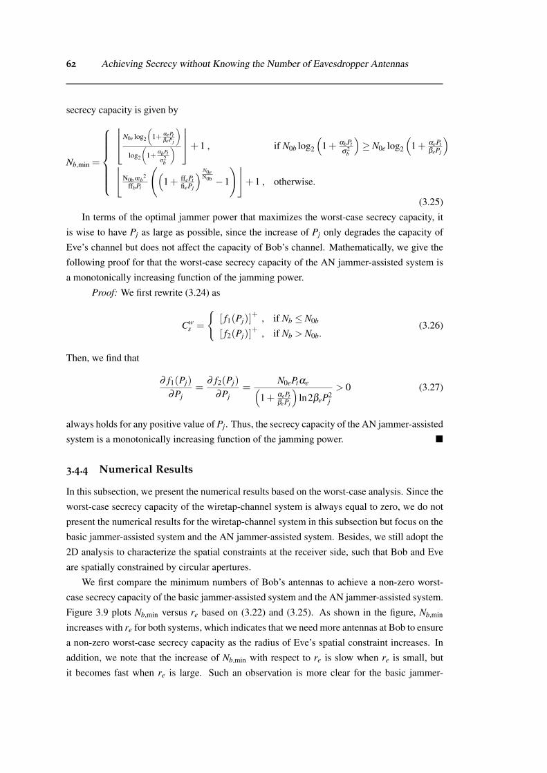
62 Achieving Secrecy without Knowing the Number of Eavesdropper Antennas
secrecy capacity is given by
Nb,min =
N0e log2
(1+ αePt
βePj
)log2
(1+ αbPt
σ2b
)+ 1 , if N0b log2
(1+ αbPt
σ2b
)≥ N0e log2
(1+ αePt
βePj
)⌊
N0b œb2
ffbPt
((1+ ffePt
fiePj
) N0eN0b −1
)⌋+ 1 , otherwise.
(3.25)
In terms of the optimal jammer power that maximizes the worst-case secrecy capacity, it
is wise to have Pj as large as possible, since the increase of Pj only degrades the capacity of
Eve’s channel but does not affect the capacity of Bob’s channel. Mathematically, we give the
following proof for that the worst-case secrecy capacity of the AN jammer-assisted system is
a monotonically increasing function of the jamming power.
Proof: We first rewrite (3.24) as
Cws =
{[ f1(Pj)]
+ , if Nb ≤ N0b
[ f2(Pj)]+ , if Nb > N0b.
(3.26)
Then, we find that
∂ f1(Pj)
∂Pj=
∂ f2(Pj)
∂Pj=
N0ePtαe(1+ αePt
βePj
)ln2βeP2
j
> 0 (3.27)
always holds for any positive value of Pj. Thus, the secrecy capacity of the AN jammer-assisted
system is a monotonically increasing function of the jamming power. �
3.4.4 Numerical Results
In this subsection, we present the numerical results based on the worst-case analysis. Since the
worst-case secrecy capacity of the wiretap-channel system is always equal to zero, we do not
present the numerical results for the wiretap-channel system in this subsection but focus on the
basic jammer-assisted system and the AN jammer-assisted system. Besides, we still adopt the
2D analysis to characterize the spatial constraints at the receiver side, such that Bob and Eve
are spatially constrained by circular apertures.
We first compare the minimum numbers of Bob’s antennas to achieve a non-zero worst-
case secrecy capacity of the basic jammer-assisted system and the AN jammer-assisted system.
Figure 3.9 plots Nb,min versus re based on (3.22) and (3.25). As shown in the figure, Nb,min
increases with re for both systems, which indicates that we need more antennas at Bob to ensure
a non-zero worst-case secrecy capacity as the radius of Eve’s spatial constraint increases. In
addition, we note that the increase of Nb,min with respect to re is slow when re is small, but
it becomes fast when re is large. Such an observation is more clear for the basic jammer-
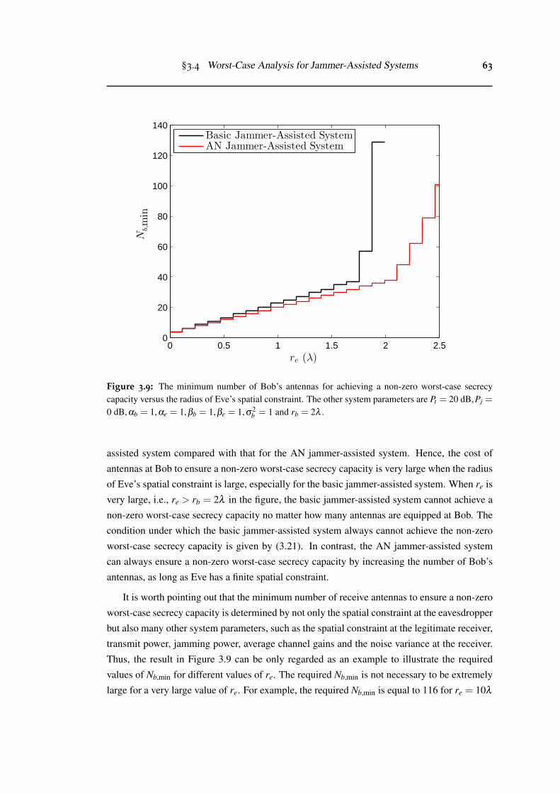
§3.4 Worst-Case Analysis for Jammer-Assisted Systems 63
0 0.5 1 1.5 2 2.50
20
40
60
80
100
120
140
re (λ)
Nb,min
Basic Jammer-Assisted SystemAN Jammer-Assisted System
Figure 3.9: The minimum number of Bob’s antennas for achieving a non-zero worst-case secrecycapacity versus the radius of Eve’s spatial constraint. The other system parameters are Pt = 20 dB,Pj =
0 dB,αb = 1,αe = 1,βb = 1,βe = 1,σ2b = 1 and rb = 2λ .
assisted system compared with that for the AN jammer-assisted system. Hence, the cost of
antennas at Bob to ensure a non-zero worst-case secrecy capacity is very large when the radius
of Eve’s spatial constraint is large, especially for the basic jammer-assisted system. When re is
very large, i.e., re > rb = 2λ in the figure, the basic jammer-assisted system cannot achieve a
non-zero worst-case secrecy capacity no matter how many antennas are equipped at Bob. The
condition under which the basic jammer-assisted system always cannot achieve the non-zero
worst-case secrecy capacity is given by (3.21). In contrast, the AN jammer-assisted system
can always ensure a non-zero worst-case secrecy capacity by increasing the number of Bob’s
antennas, as long as Eve has a finite spatial constraint.
It is worth pointing out that the minimum number of receive antennas to ensure a non-zero
worst-case secrecy capacity is determined by not only the spatial constraint at the eavesdropper
but also many other system parameters, such as the spatial constraint at the legitimate receiver,
transmit power, jamming power, average channel gains and the noise variance at the receiver.
Thus, the result in Figure 3.9 can be only regarded as an example to illustrate the required
values of Nb,min for different values of re. The required Nb,min is not necessary to be extremely
large for a very large value of re. For example, the required Nb,min is equal to 116 for re = 10λ
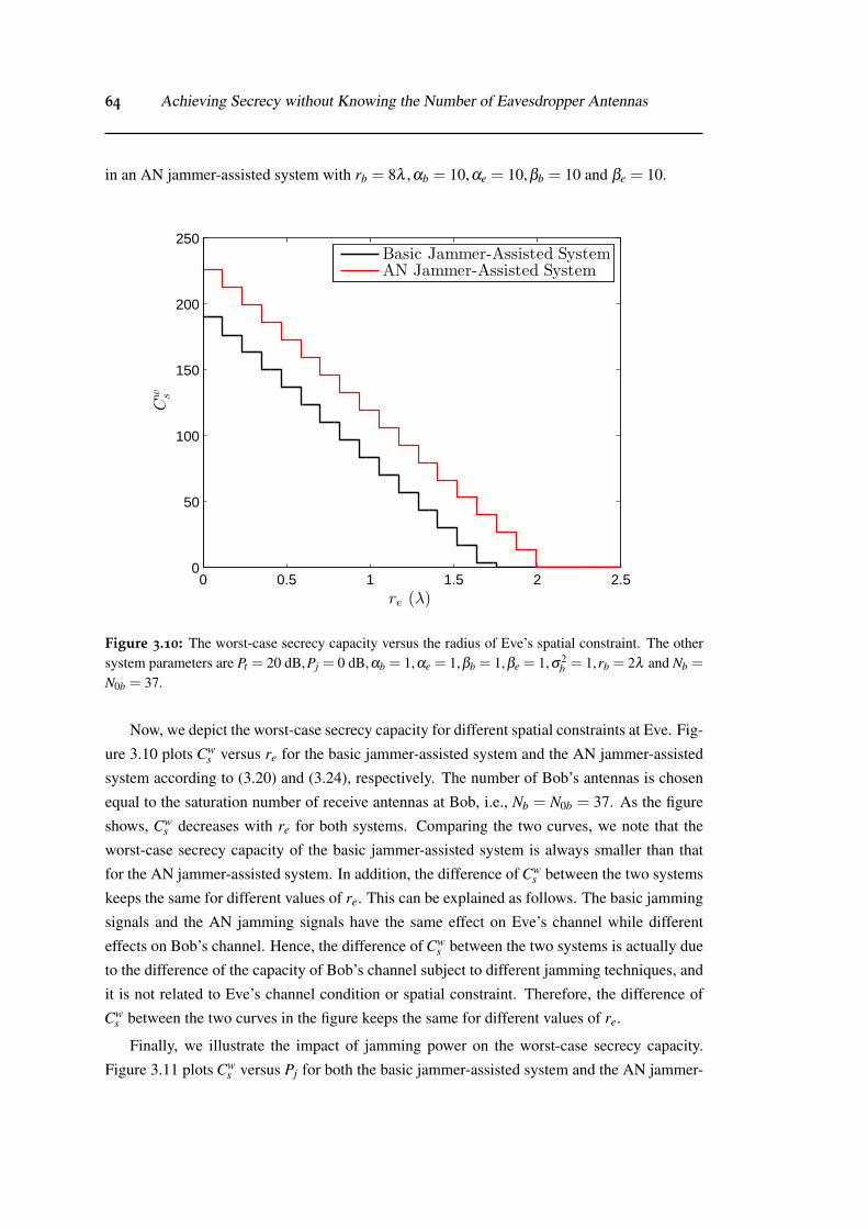
64 Achieving Secrecy without Knowing the Number of Eavesdropper Antennas
in an AN jammer-assisted system with rb = 8λ ,αb = 10,αe = 10,βb = 10 and βe = 10.
0 0.5 1 1.5 2 2.50
50
100
150
200
250
re (λ)
Cw s
Basic Jammer-Assisted SystemAN Jammer-Assisted System
Figure 3.10: The worst-case secrecy capacity versus the radius of Eve’s spatial constraint. The othersystem parameters are Pt = 20 dB,Pj = 0 dB,αb = 1,αe = 1,βb = 1,βe = 1,σ2
b = 1,rb = 2λ and Nb =
N0b = 37.
Now, we depict the worst-case secrecy capacity for different spatial constraints at Eve. Fig-
ure 3.10 plots Cws versus re for the basic jammer-assisted system and the AN jammer-assisted
system according to (3.20) and (3.24), respectively. The number of Bob’s antennas is chosen
equal to the saturation number of receive antennas at Bob, i.e., Nb = N0b = 37. As the figure
shows, Cws decreases with re for both systems. Comparing the two curves, we note that the
worst-case secrecy capacity of the basic jammer-assisted system is always smaller than that
for the AN jammer-assisted system. In addition, the difference of Cws between the two systems
keeps the same for different values of re. This can be explained as follows. The basic jamming
signals and the AN jamming signals have the same effect on Eve’s channel while different
effects on Bob’s channel. Hence, the difference of Cws between the two systems is actually due
to the difference of the capacity of Bob’s channel subject to different jamming techniques, and
it is not related to Eve’s channel condition or spatial constraint. Therefore, the difference of
Cws between the two curves in the figure keeps the same for different values of re.
Finally, we illustrate the impact of jamming power on the worst-case secrecy capacity.
Figure 3.11 plots Cws versus Pj for both the basic jammer-assisted system and the AN jammer-
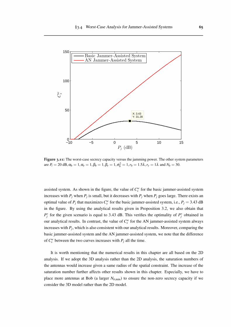
§3.4 Worst-Case Analysis for Jammer-Assisted Systems 65
−10 −5 0 5 10 150
50
100
150
Pj (dB)
Cw s
X: 3.43Y: 31.28
Basic Jammer-Assisted SystemAN Jammer-Assisted System
Figure 3.11: The worst-case secrecy capacity versus the jamming power. The other system parametersare Pt = 20 dB,αb = 1,αe = 1,βb = 1,βe = 1,σ2
b = 1,rb = 1.5λ ,re = 1λ and Nb = 30.
assisted system. As shown in the figure, the value of Cws for the basic jammer-assisted system
increases with Pj when Pj is small, but it decreases with Pj when Pj goes large. There exists an
optimal value of Pj that maximizes Cws for the basic jammer-assisted system, i.e., Pj = 3.43 dB
in the figure. By using the analytical results given in Proposition 3.2, we also obtain that
P∗j for the given scenario is equal to 3.43 dB. This verifies the optimality of P∗j obtained in
our analytical results. In contrast, the value of Cws for the AN jammer-assisted system always
increases with Pj, which is also consistent with our analytical results. Moreover, comparing the
basic jammer-assisted system and the AN jammer-assisted system, we note that the difference
of Cws between the two curves increases with Pj all the time.
It is worth mentioning that the numerical results in this chapter are all based on the 2D
analysis. If we adopt the 3D analysis rather than the 2D analysis, the saturation numbers of
the antennas would increase given a same radius of the spatial constraint. The increase of the
saturation number further affects other results shown in this chapter. Especially, we have to
place more antennas at Bob (a larger Nb,min) to ensure the non-zero secrecy capacity if we
consider the 3D model rather than the 2D model.
66 Achieving Secrecy without Knowing the Number of Eavesdropper Antennas
3.5 Summary
In this chapter, we introduced the spatial constraint into physical layer security for multi-
antenna systems, which provides an approach to study the secrecy capacity without knowing
the number of eavesdropper antennas. We considered basic secure communication systems
with spatial constraints at the receiver side. Specifically, we studied the wiretap-channel sys-
tem, the basic jammer-assisted system and the AN jammer-assisted system, and derived the
expressions for secrecy capacity of each system. We found that a non-zero worst-case secrecy
capacity is achievable with the assist of jamming signals, even if the eavesdropper is equipped
with infinite number of antennas. Moreover, the optimal jamming power that maximizes the
worst-case secrecy capacity was obtained. We highlight that the major contribution of this
chapter is to address the practically important problem of how to study secure communica-
tions without knowing the number of eavesdropper antennas, and hope the work in this chapter
can be a good inspiration for future researchers to design novel physical layer techniques to
efficiently secure wireless communications without the information of eavesdropper antennas.
Chapter 4
Base Station Cooperation forConfidential Broadcasting inMulti-Cell Networks
4.1 Introduction
The previous two chapters studied the physical layer security with practical assumptions in
order to enhance the practicality of physical layer security. In the following two chapters, we
aim to improve the applicability of physical layer security in practical networks.
Apart from the wiretap-channel systems, there exists another branch of research focusing
on the physical layer security in multi-antenna broadcast networks, and aiming at achieving
confidential broadcasting. Confidential broadcasting requires multiple messages to be se-
curely broadcasted to multiple users in the network, and each message is intended for one
user but needs to keep secret from the other users. We note that the solution to confiden-
tially broadcasting messages in multi-cell networks has not been addressed in the literature,
although the confidential broadcasting in a single isolated cell has been elaborately studied
in, e.g., [41, 43, 44, 45]. In multi-cell networks, the control of inter-cell information leakage
and interference becomes very important, besides the intra-cell information leakage and inter-
ference. This makes the current techniques achieving confidential broadcasting in single-cell
networks not applicable to multi-cell networks.
In this chapter, we provide an effective solution to tackle the challenging problem of multi-
cell confidential broadcasting. To this end, we design linear precoders at BSs that achieve
confidential broadcasting in the multi-cell network. Two forms of cooperation at the BSs, i.e.,
the MCP and the CBf, are taken into consideration such that the BSs can share control signals,
CSI and/or messages to cooperatively serve users in multiple cells. In the MCP, the BSs fully
cooperate such that they share their CSI and messages to transmit. Alternatively, in the CBf
the BSs “partially" cooperate. As such, they do not share their messages to transmit but allow
users to feed back the CSI to the cross-cell BS. In practice, the MCP is appropriate for the
67
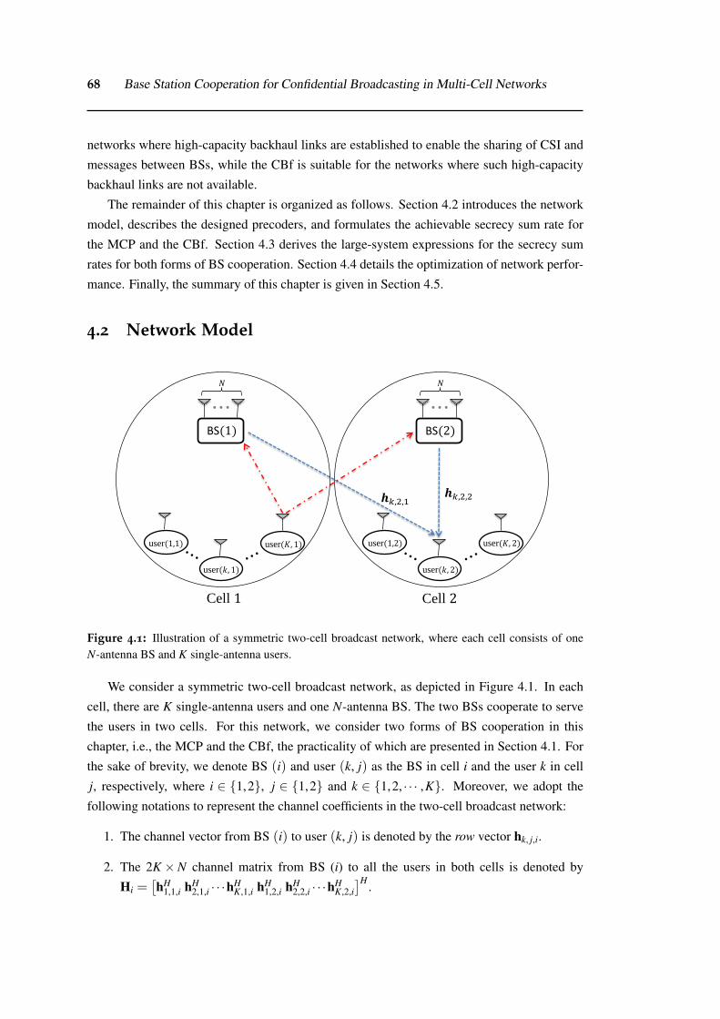
68 Base Station Cooperation for Confidential Broadcasting in Multi-Cell Networks
networks where high-capacity backhaul links are established to enable the sharing of CSI and
messages between BSs, while the CBf is suitable for the networks where such high-capacity
backhaul links are not available.
The remainder of this chapter is organized as follows. Section 4.2 introduces the network
model, describes the designed precoders, and formulates the achievable secrecy sum rate for
the MCP and the CBf. Section 4.3 derives the large-system expressions for the secrecy sum
rates for both forms of BS cooperation. Section 4.4 details the optimization of network perfor-
mance. Finally, the summary of this chapter is given in Section 4.5.
4.2 Network Model
𝑁
⋯ BS(1)
Cell 1
user(𝐾, 1)
Type equation here. user(𝑘, 1)
user(1,1)
𝑁
⋯
BS(2)
Cell 2
user(𝐾, 2)
Type equation here. user(𝑘, 2)
user(1,2)
𝒉𝑘,2,2
,2,
Figure 4.1: Illustration of a symmetric two-cell broadcast network, where each cell consists of oneN-antenna BS and K single-antenna users.
We consider a symmetric two-cell broadcast network, as depicted in Figure 4.1. In each
cell, there are K single-antenna users and one N-antenna BS. The two BSs cooperate to serve
the users in two cells. For this network, we consider two forms of BS cooperation in this
chapter, i.e., the MCP and the CBf, the practicality of which are presented in Section 4.1. For
the sake of brevity, we denote BS (i) and user (k, j) as the BS in cell i and the user k in cell
j, respectively, where i ∈ {1,2}, j ∈ {1,2} and k ∈ {1,2, · · · ,K}. Moreover, we adopt the
following notations to represent the channel coefficients in the two-cell broadcast network:
1. The channel vector from BS (i) to user (k, j) is denoted by the row vector hk, j,i.
2. The 2K ×N channel matrix from BS (i) to all the users in both cells is denoted by
Hi =[hH
1,1,i hH2,1,i · · ·hH
K,1,i hH1,2,i hH
2,2,i · · ·hHK,2,i]H .
§4.2 Network Model 69
3. The channel vector from both BSs to user (k, j) is denoted by hk, j = [hk, j,1 hk, j,2].
4. The 2K× 2N channel matrix from both BSs to all the users in both cells is denoted by
H =[hH
1,1 hH2,1 · · ·hH
K,1 hH1,2 hH
2,2 · · ·hHK,2]H .
5. The channel vector between a user and the same-cell BS is denoted by hk, j, j.
6. The channel vector between a user and the cross-cell BS is denoted by hk, j, j where j = 1
if j = 2 and j = 2 if j = 1.
We assume that the antennas at the BSs and the users are sufficiently spaced apart such
that all links between the transmit and receive antennas are uncorrelated. We also assume
that the data are transmitted over the block fading channel where the coherence time of the
channel is larger than the symbol interval. In addition, we consider a homogenous scenario
where all users in the same cell to a BS have the same average power. This is a widely-adopted
consideration for multi-user networks where the users in the same cell are located at the same
distance away from the BS. A practical example of this scenario is that the users in the same
cell are close together, e.g., in an office building, but far from the BS. Then, the channels
between a user and the same-cell BS are modeled as i.i.d. complex Gaussian variables with
zero mean and unit variance, i.e., hk, j, j ∼ CN (0,IN), whereas the channels between a user
and the cross-cell BS are modeled as i.i.d. complex Gaussian variables with zero mean and
variance ε , i.e., hk, j, j ∼ CN (0,εIN). Here, 0 < ε ≤ 1 represents the cross-cell interference
level, which characterizes the severity of interference between two cells [60, 84]. In addition,
we assume that each user (k, j) perfectly knows hk, j and feeds back hk, j, j to the same-cell BS
and hk, j, j to the cross-cell BS through corresponding uplink channels. Finally, we assume that
the BSs perfectly recover the CSI from feedback information. We note that this chapter adopts
the assumption of perfect CSI at the BS. If channel estimation errors exist, the achievable
secrecy rates of the proposed schemes would become worse. As such, the achievable secrecy
rates derived in this chapter can be treated as an upper bound on the achievable secrecy rates
for the network with channel estimation errors.
Given the aforementioned assumptions and notations, the received signal at user (k, j) is
given by
yk, j = hk, j,1x1 +hk, j,2x2 + nk, j, (4.1)
where xi ∈ CN×1, i ∈ {1,2} is the transmitted data from BS (i) and nk, j ∼ CN (0,σ2d ) is the
AWGN at user (k, j). We clarify that xi consists of the linearly precoded symbols for the users
to be served. We also clarify that the generation of xi depends on the form of BS cooperation
considered, as will be detailed in Sections 4.2.2 and 4.2.3. The vector equation of received
signals at all users is given by
y = H1x1 +H2x2 +n, (4.2)
70 Base Station Cooperation for Confidential Broadcasting in Multi-Cell Networks
where y = [y1,1 y2,1 · · ·yK,1 y1,2 y2,2 · · ·yK,2]T and n = [n1,1 n2,1 · · ·nK,1 n1,2 n2,2 · · ·nK,2]
T .
4.2.1 Confidential Broadcasting and Performance Metric
The aim of this chapter is to design linear precoders to achieve confidential broadcasting in the
two-cell broadcast network. To meet the requirement of confidential broadcasting, the message
for each user (k, j) needs to be securely transmitted such that the unintended users obtain zero
information. We consider a worst-case scenario in the two-cell network. In such a scenario,
we assume that for the message to each user (k, j), all remaining 2K−1 users in both cells act
as eavesdroppers, and they jointly eavesdrop on the message in a collaborative manner. The
cooperating eavesdroppers decode their own signals and share them with each other. It follows
that the cooperating eavesdroppers are able to perform interference cancellation, leaving only
the signal for the intended user. The alliance of 2K− 1 cooperating eavesdroppers is equiva-
lent to a single eavesdropper with 2K−1 distributed receive antennas, which is denoted by the
eavesdropper (k, j). The consideration of the worst-case scenario is motivated by the fact that
the malicious behaviors of the potential eavesdroppers in the network are not fully controllable
or predictable at the BSs. As a result, the weaker assumption of non-colluding eavesdroppers
(or equivalently, eavesdroppers are interfered by each other) cannot lead to any true guarantee
of security. Furthermore, we clarify that intentionally sharing the received messages by po-
tential eavesdroppers does not disobey the rule of confidential broadcasting. This is due to the
fact that confidential broadcasting requires the BSs to securely transmit messages to each user,
but does not control the users’ behaviors after receiving messages. Due to the aforementioned
necessity, we highlight that the consideration of the worst-case scenario is widely adopted in
designing confidential broadcasting networks, e.g., [41, 43, 44, 45].
The secrecy performance in the two-cell broadcast network is measured by the secrecy sum
rate, denoted by Rs. It is mathematically formulated as
Rs =2
∑j=1
K
∑k=1
Rk j, (4.3)
where Rk j is the secrecy rate for the message to user (k, j). According to the principles of
physically layer security, Rk j is given by
Rk j =[log2 (1+SINRk, j)− log2
(1+SINRk, j
)]+, (4.4)
where SINRk, j and SINRk, j denote the signal-to-interference-plus-noise ratios (SINRs) at the
intended user (k, j) and the eavesdropper (k, j), respectively.
Note that we assume that the eavesdroppers’ CSI is available at the transmitter in this chap-
ter, which is different from the CSI assumptions in the previous two chapters. This is because
§4.2 Network Model 71
that we study the scenario where potential eavesdroppers are users served by the transmitter
in this chapter, while in the the previous two chapters we consider the scenarios where the
eavesdropper(s) are external and not served by the transmitter.
4.2.2 Multi-Cell Processing with RCI Precoder
In the MCP, the two BSs fully cooperate to serve the users in the two cells based on the mutually
shared CSI and messages to transmit. We note that the two-cell broadcast network with the
MCP may appear to be similar to a single-cell broadcast network with 2N transmit antennas
and 2K single-antenna users. However, it is worth mentioning that the design of transmission
schemes and the corresponding analysis for confidential broadcasting in the MCP, which take
the cross-cell interference level ε into consideration, are fundamentally different from those
for confidential broadcasting in a single cell, e.g., [43]. As mentioned before, the cross-cell
interference level, ε , characterizes the severity of interference between two cells. For the
single-cell network considered in [43], the average SNRs for all channels between the BS and
the users are assumed to be the same. This implies that all channels are identically distributed.
Different from [43], for considered the MCP, the average SNRs of the same-cell channels are
different from the average SNRs of the cross-cell channels. For example, if the average SNRs
of the same-cell channels are equal to 1, the average SNRs of the cross-cell channels are equal
to ε , where 0 < ε ≤ 1. This implies that all channels are non-identically distributed. Therefore,
the large-system analysis of the secrecy sum rate in [43] cannot be directly applied in the MCP,
and new large-system analysis needs to be conducted to address the non-identically distributed
channel coefficients. We find that when ε = 1, the MCP reduces to the single-cell network,
which shows that the result in [43] is a special case of the result for the MCP.
We next detail the precoder design for the MCP. In our design, the RCI precoder [59] is
adopted at BSs to achieve confidential broadcasting. As a linear precoder, the RCI precoder
has a low signal-processing complexity and the ability of controlling the information leakage
as well as the interference amongst the users [43, 45]. As per the rules of the RCI precoder,
the precoding vector for the message to user (k, j) is given by
wk, j = c(HHH+αI2N
)−1 hHk, j, (4.5)
where c is a scaling factor to ensure the power constraint at BSs and α is a real non-negative
regularization parameter. Notably, the regularization parameter α achieves a tradeoff between
the signal power at the intended receiver and the amount of information leakage as well as
interference amongst users. Using wk, j, the transmitted data vector x = [x1;x2] is written as
x =2
∑j=1
K
∑k=1
wk, jsk, j, (4.6)
72 Base Station Cooperation for Confidential Broadcasting in Multi-Cell Networks
where sk, j denotes the message to be transmitted to user (k, j). We assume that the messages
for different users are independent and impose a unit average power constraint on sk, j such that
E{
ssH}= I2K with s = [s1;s2] and s j = [s1, j s2, j · · ·sK, j]
T . We also assume that the BSs are
subject to an average sum-power constraint such that E{‖x‖2
}= Pt . Accordingly, the scaling
factor c is determined by
c2 =Pt
Tr((HHH+αI2N)
−2 HHH) . (4.7)
Based on (4.5) and (4.6), the received signal at the intended user (k, j) is written as
yk, j = chk, j(HHH+αI2N
)−1 HHs+ nk j
= chk, j(HHH+αI2N
)−1 hHk, jsk, j + chk, j
(HHH+αI2N
)−1 HHk, jsk, j + nk j, (4.8)
where Hk, j and sk, j are obtained from H and s by removing the row corresponding to user
(k, j), respectively. Moreover, the received signal vector at the eavesdropper (k, j) is written
as
yk, j = cHk, j
(HHH+αI2N
)−1 hHk, jsk, j +nk, j, (4.9)
where yk, j and nk, j are obtained from y and n by removing the row corresponding to user (k, j),
respectively. Based on (4.8) and (4.9), the SINRs for the message sk, j at the intended user (k, j)
and the eavesdropper (k, j) are given by
SINRk, j =c2∣∣∣hk, j
(HHH+αI2N
)−1 hHk, j
∣∣∣2c2ψ +σ2
d(4.10)
and
SINRk, j =c2∣∣∣Hk, j
(HHH+αI2N
)−1 hHk, j
∣∣∣2σ2
d, (4.11)
respectively, where
ψ =hk, j(HHH+αI2N
)−1HHk, jHk, j
(HHH+αI2N
)−1hHk, j. (4.12)
As such, the secrecy sum rate achieved by the RCI precoder for the MCP is obtained as
Rs,MCP =2
∑j=1
K
∑k=1
log2
1+
c2∣∣∣hk, j(HH H+αI2N)
−1hH
k, j
∣∣∣2c2hk, j(HH H+αI2N)
−1HHk, j
Hk, j(HH H+αI2N)−1hH
k, j+σ2d
1+c2|Hk, j(HH H+αI2N)
−1hHk, j|
2
σ2d
+
. (4.13)
§4.2 Network Model 73
4.2.3 Coordinated Beamforming with Generalized RCI Precoder
In the CBf, the two BSs partially cooperate based on the CSI from all users. Since the BSs
do not know the messages for the cross-cell users, they only transmit data for the users in
their own cells. Also, the two BSs cooperate to control the information leakage in both cells.
Furthermore, they cooperate to control the interference power amongst the users in both cells
(or equivalently, the received signal power at unintended users) by properly designing the
precoder and wisely choosing the regularization parameter α [60, 85].
We now detail the precoder design for the CBf. In this design, we consider the generalized
RCI precoder [60] at BSs to achieve confidential broadcasting. Note that the generalized RCI
precoder has never been investigated as a method to achieve confidential broadcasting. More-
over, the principle of the generalized RCI precoder is different from that of the RCI precoder.
We clarify that the primary benefit of using the generalized RCI precoder for the CBf is that
each BS in this precoder controls the interference and information leakage amongst the users
not only in the same cell but also in the cross cell. If we adopt the RCI precoder in the CBf, as
we do in the MCP, each BS transmits data and controls the interference and information leak-
age amongst the users only in the same cell. As per the rules of the generalized RCI precoder,
the precoding vector for the message to user (k, j) is given by
wk, j = c jwk, j
= c j
(∑
(l,m) 6=(k, j)
hHl,m, jhl,m, j +αIN
)−1
hHk, j, j, (4.14)
where c j is the scaling factor to ensure the power constraint at BS ( j) and α is the real non-
negative regularization parameter achieving the tradeoff between the signal power at the in-
tended receiver and the amount of information leakage as well as interference amongst users.
The transmitted data vector at the BS ( j) is written as
x j =K
∑k=1
wk, jsk, j, (4.15)
where sk, j denotes the message to be transmitted to user (k, j) with the same property as that
in the MCP. From (4.14) and (4.15), we find that BS ( j) only requires the CSI from itself to
users, hk,i, j, to construct the precoding matrix. That is, BS ( j) does not need the CSI from the
other BS ( j) to users, hk,i, j, for the precoding matrix construction. Different from the average
sum-power constraint for two BSs in the MCP, we consider in the CBf that each BS is subject
to an average power constraint, such that E{‖x j‖2
}= Pj. Then the total power constraint for
two BSs is given by Pt = P1 +P2. Here we assume the same average power constraint at both
74 Base Station Cooperation for Confidential Broadcasting in Multi-Cell Networks
BSs, i.e., P1 = P2 = P = Pt/2. Hence, the scaling factor c j in (4.14) is determined by
c2j =
Pj
∑Kk=1
∥∥wk, j∥∥2 . (4.16)
Based on (4.14) and (4.15), the received signal at the intended user (k, j) is written as
yk, j = hk, j, jwk, jsk, j + ∑(k′, j′) 6=(k, j)
hk, j, j′wk′, j′sk′, j′+ nk, j. (4.17)
Moreover, the received signal vector at the eavesdropper (k, j) is written as
yk, j = Hk, j, jwk, jsk, j +nk, j. (4.18)
where Hk, j, j and nk, j are obtained from H j and n by removing the row corresponding to user
(k, j), respectively. Based on (4.17) and (4.18), the SINRs for the message sk, j at the intended
user (k, j) and the eavesdropper (k, j) are given by
SINRk, j =c2
j
∣∣hk, j, jwk, j∣∣2
∑(k′, j′) 6=(k, j) c2j′∣∣hk, j, j′wk′, j′
∣∣2 +σ2d
(4.19)
and
SINRk, j =∑(k′, j′) 6=(k, j) c2
j
∣∣hk′, j′, jwk, j∣∣2
σ2d
, (4.20)
respectively. Aided by (4.19) and (4.20), the secrecy sum rate achieved by the generalized RCI
precoder for the CBf is obtained as
Rs,CBf =2
∑j=1
K
∑k=1
log2
1+
c2j |hk, j, jwk, j|2
∑(k′ , j′) 6=(k, j) c2j′ |hk, j, j′ wk′ , j′ |2+σ2
d
1+∑(k′ , j′) 6=(k, j) c2
j |hk′ , j′ , jwk, j|2σ2
d
+
. (4.21)
It is evident that the secrecy sum rates in (4.13) and (4.21) depend on the realization of
each channel, hk, j,i. Based on them, we can only evaluate the secrecy performance by time-
consuming numerical simulations. This motivates us to seek channel-independent expressions
that reduce the complexity of performance evaluations. Therefore, in the next section we
resort to the large-system analysis to explicitly characterize the secrecy sum rate of confidential
broadcasting in the two-cell broadcast network.
§4.3 Secrecy Sum Rate in the Large-System Regime 75
4.3 Secrecy Sum Rate in the Large-System Regime
In this section, we derive channel-independent expressions for the secrecy sum rate of the two-
cell broadcast network in the large-system regime. In such a regime, both the number of users
in each cell, K, and the number of transmit antennas at each BS, N, approach infinity with
a fixed ratio, β = K/N. Besides, we denote γ = Pt/(2σ2d ) = P/σ2
d as the average transmit
SNR at each BS. As will be shown later in numerical simulations, the analytical result in the
large-system regime can accurately approximate the secrecy sum rate of the network even with
finite K and N.
4.3.1 Large-System Analysis
In the large-system analysis for the symmetric two-cell network with K,N → ∞, the secrecy
rate for all messages sk, j converge to the same non-random function. This function does not
depend on the realization of each channel hk, j,i. Thus, the secrecy sum rate is analytically
approximated by
R∞s = 2K
(R∞
k, j)= 2K
[log2
1+SINR∞k, j
1+SINR∞
k, j
]+, (4.22)
where R∞k, j denotes the large-system secrecy rate for each user, SINR∞
k, j and SINR∞
k, j denote the
large-system approximations of the SINRs at the intended user and the eavesdropper, respec-
tively.
In the following Theorem 4.1 and Theorem 4.2, we present the large-system secrecy sum
rate achieved by the RCI precoder for the MCP and the large-system secrecy sum rate achieved
by the generalized RCI precoder for the CBf, respectively.
Theorem 4.1. In the large-system regime, the secrecy sum rate achieved by the RCI precoder
for the MCP converges in probability to a deterministic quantity given by
R∞s,MCP =
2K
log2
1+(1+ε)γg(β ,ρM)1+
ρMβ
(1+g(β ,ρM ))2
(1+ε)γ+(1+g(β ,ρM ))2
1+ (1+ε)γ
(1+g(β ,ρM ))2
+
, if α 6= 0
2K log2
(1+ (1−β )(1+ε)γ
β
), if α = 0 and β ≤ 1
2K[log2
(β 3(β+(β−1)(1+ε)γ)
(β 2+(β−1)2(1+ε)γ)2
)]+, if α = 0 and β > 1.
(4.23)
where ρM = (1+ ε)−1α/N and g(β ,ρM) is the solution of x to x =(
ρM + β
1+x
)−1.
Proof: See Appendix C.1. �
Theorem 4.2. In the large-system regime, the secrecy sum rate achieved by the generalized
76 Base Station Cooperation for Confidential Broadcasting in Multi-Cell Networks
RCI precoder for the CBf converges almost surely to a deterministic quantity given by
R∞s,CBf =
2K
log2
1+
Λβ
(ρC+
βε
(1+εΛ)2+
β
(1+Λ)2
)1γ +
ε
(1+εΛ)2+ 1(1+Λ)2
1+γ
(ε
(1+εΛ)2+ 1
(1+Λ)2
)+
, if α 6= 0
2K log2
(1+ (1−2β )γ
β
), if α = 0 and β ≤ 0.5
2K
log2
1+
Λ0β
(βε
(1+εΛ0)2 +
β
(1+Λ0)2
)1γ +
ε
(1+εΛ0)2 + 1
(1+Λ0)2
1+γ
(ε
(1+εΛ0)2 +
1(1+Λ0)
2
)+
, if α = 0 and β > 0.5.
(4.24)
where ρC = α/N, Λ is the solution of x to x =(
ρC + βε
1+εx +β
1+x
)−1and Λ0 is the solution
of x to x =(
βε
1+εx +β
1+x
)−1.
Proof: See Appendix C.2. �
We provide several remarks about the large-system secrecy sum rates derived in Theo-
rems 4.1 and 4.2, as follows:
Remark 4.1. Theorems 4.1 and 4.2 provide closed-form and channel-independent expressions
for the large-system secrecy sum rates for the MCP and the CBf, respectively. We highlight that
these expressions eliminate the computational burden of performance evaluation incurred by
Monte Carlo simulations. Notably, these expressions allow us to evaluate and optimize the se-
crecy performance efficiently. The comparison of the optimal achievable secrecy performance
between the MCP and the CBf will be conducted in Section 4.4.1.
Remark 4.2. The results for both the MCP and the CBf contain the parameter ε , such that
they characterize the impact of the cross-cell interference level on the secrecy sum rate. This
demonstrates that the analysis of confidential broadcasting in multi-cell networks is fundamen-
tally different from that in single-cell networks which did not consider ε , e.g., [43].
Remark 4.3. We note that the result in Theorem 4.1 with ε = 1 reduces to the result for the
single-cell confidential broadcasting given in [43], which demonstrates the generality of our
analysis. This is due to the fact that the confidential broadcasting in a single cell with one
2N-antenna BS and 2K single-antenna users is equivalent to a special case of the confidential
broadcasting in the MCP.
4.3.2 Numerical Results
In this subsection, we examine the accuracy of the large-system results by comparing the large-
system secrecy sum rate, R∞s , with the average secrecy sum rate of networks with finite K and
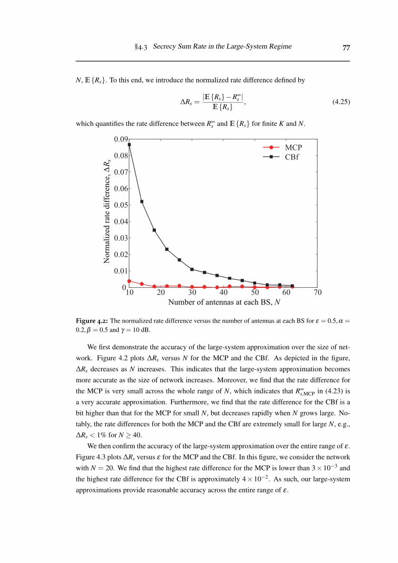
§4.3 Secrecy Sum Rate in the Large-System Regime 77
N, E{Rs}. To this end, we introduce the normalized rate difference defined by
∆Rs =|E{Rs}−R∞
s |E{Rs}
, (4.25)
which quantifies the rate difference between R∞s and E{Rs} for finite K and N.
10 20 30 40 50 60 700
0.01
0.02
0.03
0.04
0.05
0.06
0.07
0.08
0.09
Number of antennas at each BS, N
MCP
CBf
ΔRs
No
rmali
zed
rate
dif
fere
nce,
Figure 4.2: The normalized rate difference versus the number of antennas at each BS for ε = 0.5,α =
0.2,β = 0.5 and γ = 10 dB.
We first demonstrate the accuracy of the large-system approximation over the size of net-
work. Figure 4.2 plots ∆Rs versus N for the MCP and the CBf. As depicted in the figure,
∆Rs decreases as N increases. This indicates that the large-system approximation becomes
more accurate as the size of network increases. Moreover, we find that the rate difference for
the MCP is very small across the whole range of N, which indicates that R∞s,MCP in (4.23) is
a very accurate approximation. Furthermore, we find that the rate difference for the CBf is a
bit higher than that for the MCP for small N, but decreases rapidly when N grows large. No-
tably, the rate differences for both the MCP and the CBf are extremely small for large N, e.g.,
∆Rs < 1% for N ≥ 40.
We then confirm the accuracy of the large-system approximation over the entire range of ε .
Figure 4.3 plots ∆Rs versus ε for the MCP and the CBf. In this figure, we consider the network
with N = 20. We find that the highest rate difference for the MCP is lower than 3×10⁻³ and
the highest rate difference for the CBf is approximately 4× 10⁻². As such, our large-system
approximations provide reasonable accuracy across the entire range of ε .
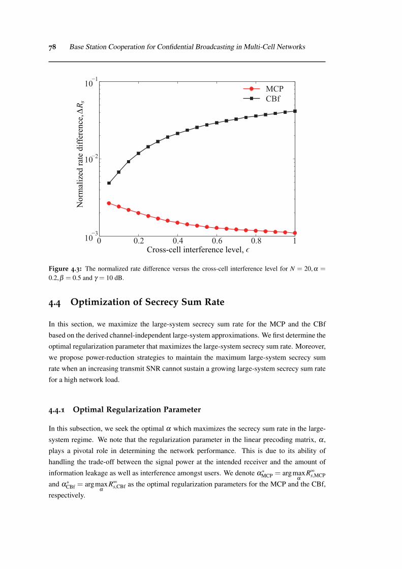
78 Base Station Cooperation for Confidential Broadcasting in Multi-Cell Networks
0 0.2 0.4 0.6 0.8 110−3
10−2
10−1
ΔR
sN
orm
ali
zed
rate
dif
fere
nce,
MCP
CBf
Cross-cell interference level, ϵ
Figure 4.3: The normalized rate difference versus the cross-cell interference level for N = 20,α =
0.2,β = 0.5 and γ = 10 dB.
4.4 Optimization of Secrecy Sum Rate
In this section, we maximize the large-system secrecy sum rate for the MCP and the CBf
based on the derived channel-independent large-system approximations. We first determine the
optimal regularization parameter that maximizes the large-system secrecy sum rate. Moreover,
we propose power-reduction strategies to maintain the maximum large-system secrecy sum
rate when an increasing transmit SNR cannot sustain a growing large-system secrecy sum rate
for a high network load.
4.4.1 Optimal Regularization Parameter
In this subsection, we seek the optimal α which maximizes the secrecy sum rate in the large-
system regime. We note that the regularization parameter in the linear precoding matrix, α ,
plays a pivotal role in determining the network performance. This is due to its ability of
handling the trade-off between the signal power at the intended receiver and the amount of
information leakage as well as interference amongst users. We denote α∗MCP = argmaxα
R∞s,MCP
and α∗CBf = argmaxα
R∞s,CBf as the optimal regularization parameters for the MCP and the CBf,
respectively.
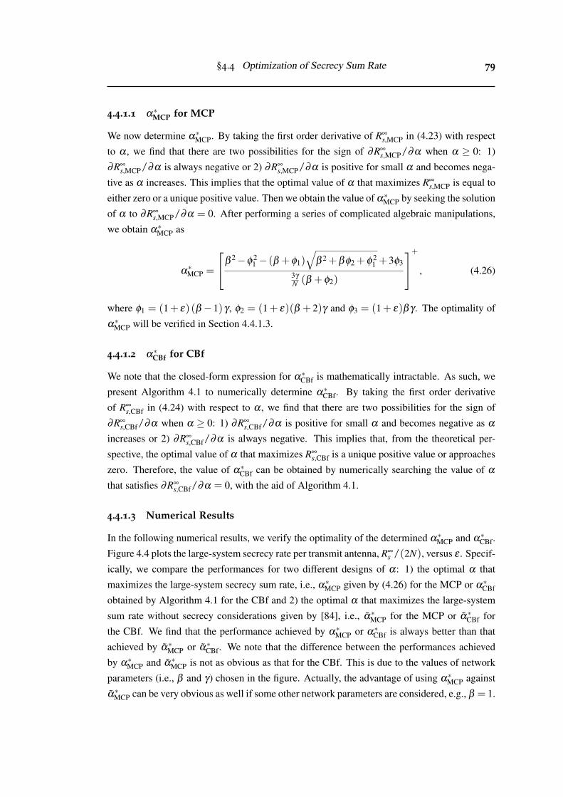
§4.4 Optimization of Secrecy Sum Rate 79
4.4.1.1 α∗MCP for MCP
We now determine α∗MCP. By taking the first order derivative of R∞s,MCP in (4.23) with respect
to α , we find that there are two possibilities for the sign of ∂R∞s,MCP/∂α when α ≥ 0: 1)
∂R∞s,MCP/∂α is always negative or 2) ∂R∞
s,MCP/∂α is positive for small α and becomes nega-
tive as α increases. This implies that the optimal value of α that maximizes R∞s,MCP is equal to
either zero or a unique positive value. Then we obtain the value of α∗MCP by seeking the solution
of α to ∂R∞s,MCP/∂α = 0. After performing a series of complicated algebraic manipulations,
we obtain α∗MCP as
α∗MCP =
β 2−φ 21 − (β +φ1)
√β 2 +βφ2 +φ 2
1 + 3φ3
3γ
N (β +φ2)
+
, (4.26)
where φ1 = (1+ ε) (β −1)γ , φ2 = (1+ ε)(β + 2)γ and φ3 = (1+ ε)βγ . The optimality of
α∗MCP will be verified in Section 4.4.1.3.
4.4.1.2 α∗CBf for CBf
We note that the closed-form expression for α∗CBf is mathematically intractable. As such, we
present Algorithm 4.1 to numerically determine α∗CBf. By taking the first order derivative
of R∞s,CBf in (4.24) with respect to α , we find that there are two possibilities for the sign of
∂R∞s,CBf/∂α when α ≥ 0: 1) ∂R∞
s,CBf/∂α is positive for small α and becomes negative as α
increases or 2) ∂R∞s,CBf/∂α is always negative. This implies that, from the theoretical per-
spective, the optimal value of α that maximizes R∞s,CBf is a unique positive value or approaches
zero. Therefore, the value of α∗CBf can be obtained by numerically searching the value of α
that satisfies ∂R∞s,CBf/∂α = 0, with the aid of Algorithm 4.1.
4.4.1.3 Numerical Results
In the following numerical results, we verify the optimality of the determined α∗MCP and α∗CBf.
Figure 4.4 plots the large-system secrecy rate per transmit antenna, R∞s /(2N), versus ε . Specif-
ically, we compare the performances for two different designs of α: 1) the optimal α that
maximizes the large-system secrecy sum rate, i.e., α∗MCP given by (4.26) for the MCP or α∗CBf
obtained by Algorithm 4.1 for the CBf and 2) the optimal α that maximizes the large-system
sum rate without secrecy considerations given by [84], i.e., α∗MCP for the MCP or α∗CBf for
the CBf. We find that the performance achieved by α∗MCP or α∗CBf is always better than that
achieved by α∗MCP or α∗CBf. We note that the difference between the performances achieved
by α∗MCP and α∗MCP is not as obvious as that for the CBf. This is due to the values of network
parameters (i.e., β and γ) chosen in the figure. Actually, the advantage of using α∗MCP against
α∗MCP can be very obvious as well if some other network parameters are considered, e.g., β = 1.

80 Base Station Cooperation for Confidential Broadcasting in Multi-Cell Networks
Algorithm 4.1 Numerical Search for α∗CBf
1: Input: f (x) =∂R∞
s,CBf∂α
(α = x);Acceptable error d (e.g., d =
10−10);Initial search point αp (e.g., αp =
1);2: Output: α∗CBf that satisfies | f (α∗CBf)| ≤
d;3: Initialize iteration counters: c = 0;4: if | f (αp)| ≤ d then5: return α∗CBf = αp; {The value of α∗CBf
is obtained.}6: end if7: if f (αp) > 0 then8: Initialize the lower bound of α∗CBf by
αl = αp;9: while f (αl + 2c) > 0 do
10: Update the lower bound by αl =αl + 2c;
11: Exponentially increase the one-sidesearch step 2c by c = c+ 1;
12: end while13: Set the upper bound of α∗CBf by αu =
αl + 2c;14: else15: Initialize the upper bound of α∗CBf by
αu = αp;16: while f (αu×10−1) < 0 do
17: Update the upper bound byαu = αu×10−1;
18: end while19: Set the lower bound of α∗CBf by
αl = αu×10−1;20: end if21: if | f (αl)| ≤ d then22: return α∗CBf = αl; {The value of α∗CBf
is obtained.}23: end if24: if | f (αu)| ≤ d then25: return α∗CBf = αu; {The value of α∗CBf
is obtained.}26: end if27: Initialize the mid-point αm = (αl +
αu)/2;28: while | f (αm)|> d do29: if f (αm) > 0 then30: αl = αm;αu = αu;31: else32: αl = αl;αu = αm;33: end if34: αm = (αl +αu)/2;35: end while36: return α∗CBf = αm; {The value of α∗CBf is
obtained.}
These observations indicate that the optimal values of α without secrecy considerations given
by [84] are no longer optimal for the networks with secrecy considerations.
Comparing the results for the MCP and the CBf, it is evident that the secrecy rate for the
MCP is in general higher than that for the CBf. This is due to the fact that the BSs in the
MCP share messages to transmit while the BSs in the CBf do not. Note that such an advantage
of secrecy rate necessitates the high-capacity backhaul links in the MCP. Moreover, we find
that the secrecy rate for the MCP increases with ε . In contrast, the secrecy rate for the CBf
decreases with ε . This observation can be explained as follows. The value of ε determines the
average channel gain from the cross-cell BS to the users. In particular, a higher ε increases the
power of the received signals from the cross-cell BS. In the MCP where BSs share messages
to transmit, a higher ε increases the received signal power at the intended user, although the
interference power at the intended user and the received signal power at the eavesdropper
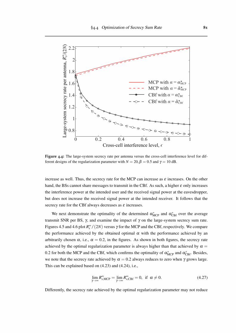
§4.4 Optimization of Secrecy Sum Rate 81
0 0.2 0.4 0.6 0.8 1
0.8
1
1.2
1.4
1.6
1.8
2
2.2
Cross-cell interference level, ϵ
Rs
Lar
ge-
syst
em s
ecre
cy r
ate
per
ante
nna,
∞/(
2N
)
α*α =
˜MCP with
MCP with MCP
α*α = MCP
α*α =
˜CBf with
CBf with CBf
α*α = CBf
Figure 4.4: The large-system secrecy rate per antenna versus the cross-cell interference level for dif-ferent designs of the regularization parameter with N = 20,β = 0.5 and γ = 10 dB.
increase as well. Thus, the secrecy rate for the MCP can increase as ε increases. On the other
hand, the BSs cannot share messages to transmit in the CBf. As such, a higher ε only increases
the interference power at the intended user and the received signal power at the eavesdropper,
but does not increase the received signal power at the intended receiver. It follows that the
secrecy rate for the CBf always decreases as ε increases.
We next demonstrate the optimality of the determined α∗MCP and α∗CBf over the average
transmit SNR per BS, γ , and examine the impact of γ on the large-system secrecy sum rate.
Figures 4.5 and 4.6 plot R∞s /(2N) versus γ for the MCP and the CBf, respectively. We compare
the performance achieved by the obtained optimal α with the performance achieved by an
arbitrarily chosen α , i.e., α = 0.2, in the figures. As shown in both figures, the secrecy rate
achieved by the optimal regularization parameter is always higher than that achieved by α =
0.2 for both the MCP and the CBf, which confirms the optimality of α∗MCP and α∗CBf. Besides,
we note that the secrecy rate achieved by α = 0.2 always reduces to zero when γ grows large.
This can be explained based on (4.23) and (4.24), i.e.,
limγ→∞
R∞s,MCP = lim
γ→∞R∞
s,CBf = 0, if α 6= 0. (4.27)
Differently, the secrecy rate achieved by the optimal regularization parameter may not reduce
82 Base Station Cooperation for Confidential Broadcasting in Multi-Cell Networks
0 5 10 15 20 25 30 350
1
2
3
4
5
6
7
8
9
= 0.8β
= 1β
= 1.2β
Transmit SNR at each BS, (dB)γ
α*α =
MCP with
MCP with MCP
0.2α =Rs
Lar
ge-
syst
em s
ecre
cy r
ate
per
ante
nna,
∞/(
2N
)
Figure 4.5: MCP: the large-system secrecy rate per antenna versus the average transmit SNR per BSfor different designs of the regularization parameter with β = 0.8,1,1.2, N = 20 and ε = 0.5.
to zero when γ is high. For the MCP, Figure 4.5 shows that the secrecy rate achieved by
α = α∗MCP monotonically increases with γ if β ≤ 1, but goes to zero at high transmit SNRs if
β > 1. For the CBf, Figure 4.6 shows that the secrecy rate achieved by α = α∗CBf monoton-
ically increases with γ if β ≤ 0.5, but goes to zero at high transmit SNRs if β > 0.5. These
observations reveal that the increase in γ benefits the secrecy performance achieved by the
optimal α , when the network load is low. We now analytically explain these observations as
follows. From the analytical results, we find that the optimal regularization parameter goes
to zero as γ increases for both the MCP and the CBf. When α → 0, we find from (4.23)
that limα→0 R∞s,MCP monotonically increases with γ if β ≤ 1, while limα→0 R∞
s,MCP approaches
to zero at high transmit SNRs if β > 1. Similarly, it is found from (4.24) that limα→0 R∞s,CBf
monotonically increases with γ if β ≤ 0.5, while limα→0 R∞s,CBf goes to zero at high transmit
SNRs if β > 0.5.
Finally, we demonstrate the advantage of the proposed precoders relative to the channel in-
version precoder in the two-cell network. The channel inversion precoder (also called as zero-
forcing precoder) is a well-known linear precoder that can eliminate the interference amongst
users in the multi-user multi-input single-output (MISO) broadcasting network where the num-
ber of users is less than or equal to the number of transmit antennas at the BS, i.e., β ≤ 1 for
the MCP or β ≤ 0.5 for the CBf. In addition, the well-known block-diagonalization (BD)
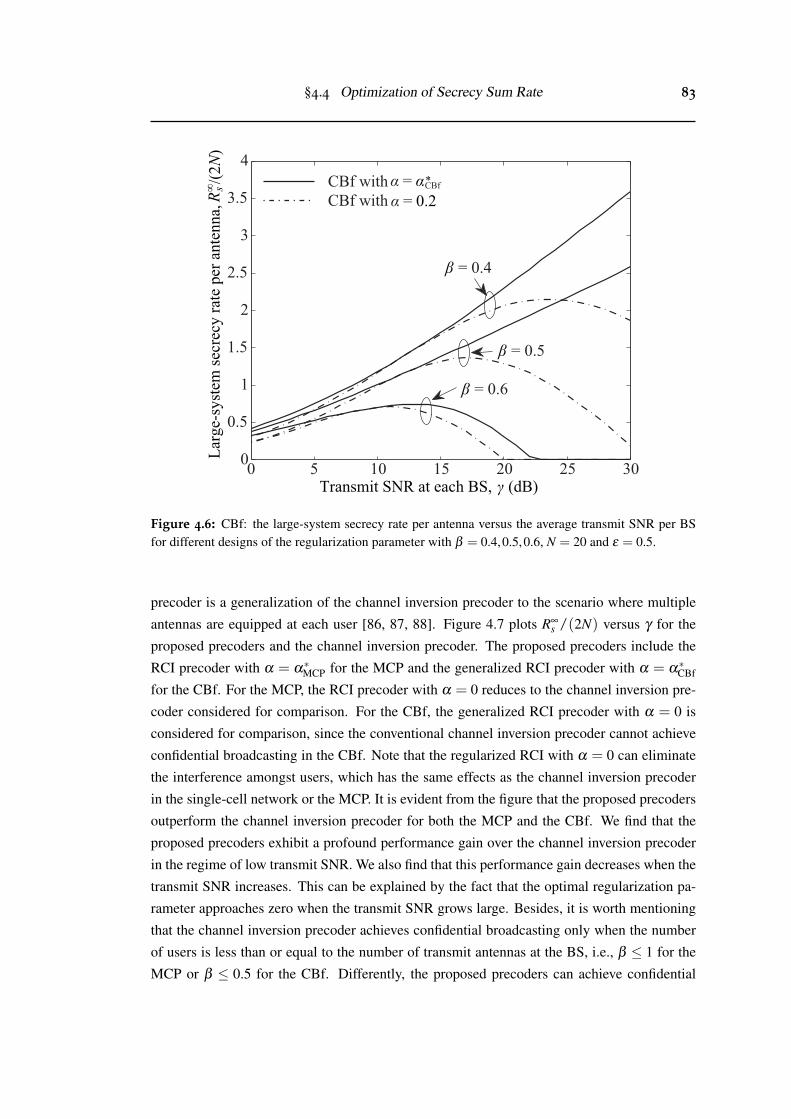
§4.4 Optimization of Secrecy Sum Rate 83
0 5 10 15 20 25 300
0.5
1
1.5
2
2.5
3
3.5
4
= 0.4β
= 0.5β
= 0.6β
Transmit SNR at each BS, (dB)γ
α*α =
CBf with
CBf with CBf
0.2α =Rs
Lar
ge-
syst
em s
ecre
cy r
ate
per
ante
nna,
∞/(
2N
)
Figure 4.6: CBf: the large-system secrecy rate per antenna versus the average transmit SNR per BSfor different designs of the regularization parameter with β = 0.4,0.5,0.6, N = 20 and ε = 0.5.
precoder is a generalization of the channel inversion precoder to the scenario where multiple
antennas are equipped at each user [86, 87, 88]. Figure 4.7 plots R∞s /(2N) versus γ for the
proposed precoders and the channel inversion precoder. The proposed precoders include the
RCI precoder with α = α∗MCP for the MCP and the generalized RCI precoder with α = α∗CBf
for the CBf. For the MCP, the RCI precoder with α = 0 reduces to the channel inversion pre-
coder considered for comparison. For the CBf, the generalized RCI precoder with α = 0 is
considered for comparison, since the conventional channel inversion precoder cannot achieve
confidential broadcasting in the CBf. Note that the regularized RCI with α = 0 can eliminate
the interference amongst users, which has the same effects as the channel inversion precoder
in the single-cell network or the MCP. It is evident from the figure that the proposed precoders
outperform the channel inversion precoder for both the MCP and the CBf. We find that the
proposed precoders exhibit a profound performance gain over the channel inversion precoder
in the regime of low transmit SNR. We also find that this performance gain decreases when the
transmit SNR increases. This can be explained by the fact that the optimal regularization pa-
rameter approaches zero when the transmit SNR grows large. Besides, it is worth mentioning
that the channel inversion precoder achieves confidential broadcasting only when the number
of users is less than or equal to the number of transmit antennas at the BS, i.e., β ≤ 1 for the
MCP or β ≤ 0.5 for the CBf. Differently, the proposed precoders can achieve confidential
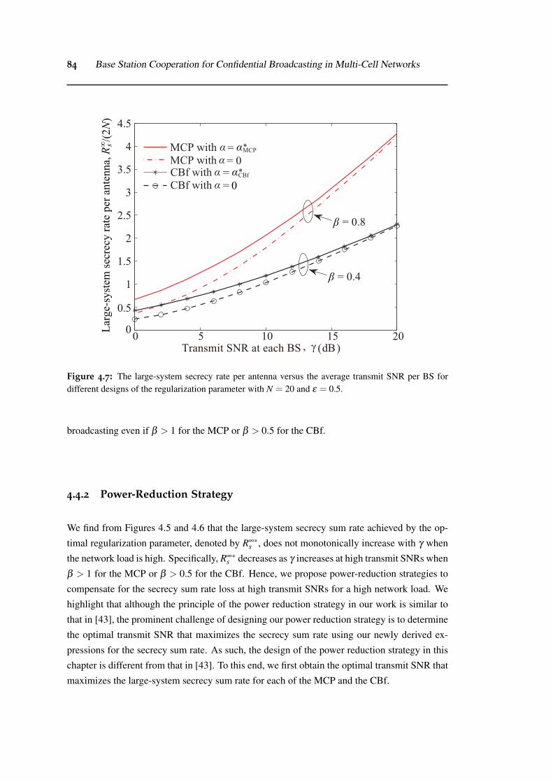
84 Base Station Cooperation for Confidential Broadcasting in Multi-Cell Networks
0 5 10 15 200
0.5
1
1.5
2
2.5
3
3.5
4
4.5
Transmit SNR at each BS , γ (dB)
α*α=MCP with MCP
α= 0MCP withα*α =CBf with CBf
α =CBf with 0
Rs
Lar
ge-
syst
em s
ecre
cy r
ate
per
ante
nna,
∞/(
2N
)
= 0.4β
= 0.8β
Figure 4.7: The large-system secrecy rate per antenna versus the average transmit SNR per BS fordifferent designs of the regularization parameter with N = 20 and ε = 0.5.
broadcasting even if β > 1 for the MCP or β > 0.5 for the CBf.
4.4.2 Power-Reduction Strategy
We find from Figures 4.5 and 4.6 that the large-system secrecy sum rate achieved by the op-
timal regularization parameter, denoted by R∞∗s , does not monotonically increase with γ when
the network load is high. Specifically, R∞∗s decreases as γ increases at high transmit SNRs when
β > 1 for the MCP or β > 0.5 for the CBf. Hence, we propose power-reduction strategies to
compensate for the secrecy sum rate loss at high transmit SNRs for a high network load. We
highlight that although the principle of the power reduction strategy in our work is similar to
that in [43], the prominent challenge of designing our power reduction strategy is to determine
the optimal transmit SNR that maximizes the secrecy sum rate using our newly derived ex-
pressions for the secrecy sum rate. As such, the design of the power reduction strategy in this
chapter is different from that in [43]. To this end, we first obtain the optimal transmit SNR that
maximizes the large-system secrecy sum rate for each of the MCP and the CBf.
§4.4 Optimization of Secrecy Sum Rate 85
4.4.2.1 Power Reduction for MCP
For the MCP, we focus on the network with β > 1, since R∞∗s,MCP does not monotonically in-
crease with γ when β > 1. We first derive the optimal transmit SNR, γ∗MCP, that maximizes the
large-system secrecy sum rate achieved by α∗MCP, i.e., γ∗MCP = argmaxγ
R∞∗s,MCP. By taking the
first-order derivative of R∞∗s,MCP with respect to γ and equating it to zero, we obtain γ∗MCP as
γ∗MCP =
β (2−β )
(1+ ε)(β −1)2 . (4.28)
Based on (4.28), we propose the power-reduction strategy to reduce the total transmit power
such that the maximum large-system secrecy sum rate is maintained. The precoding vector
with the power-reduction strategy is given by
wPR =
√
γ∗MCPγ
w∗ β > 1 and γ > γ∗MCP,
w otherwise,(4.29)
where w is the original RCI precoding vector given in (4.5) with α = α∗MCP and w∗ is the
original RCI precoding vector with α = α∗MCP at γ = γ∗MCP. We highlight that√
γ∗MCP/γ is
the power-reduction coefficient for the MCP, which is adopted when β > 1 and γ > γ∗MCP. As
such, we refer to the RCI precoder using wPR in (4.29) as the RCI-PR precoder. Note that the
reduced transmit SNR by adopting the RCI-PR precoder becomes
γPRMCP =
{γ∗MCP, β > 1 and γ > γ∗MCP
γ , otherwise.(4.30)
4.4.2.2 Power Reduction for CBf
For the CBf, we focus on the network with β > 0.5, since R∞∗s,CBf does not monotonically
increase with γ when β > 0.5. We first determine the optimal transmit SNR, γ∗CBf, that maxi-
mizes the large-system secrecy sum rate achieved by α∗CBf, i.e., γ∗CBf = argmaxγ
R∞∗s,CBf. Since the
closed-form expression for γ∗CBf cannot be derived, we obtain γ∗CBf through numerical search.
Using γ∗CBf, we propose the power-reduction strategy to reduce the total transmit power and
maintain the maximum large-system secrecy sum rate. The precoding vector with the power-
reduction strategy is given by
wPR =
√
γ∗CBfγ
w∗ β > 0.5 and γ > γ∗CBf,
w otherwise,(4.31)
where w is the original generalized RCI precoding vector given in (4.14) with α = α∗CBf and
w∗ is the original generalized RCI precoding vector with α = α∗CBf at γ = γ∗CBf. We highlight
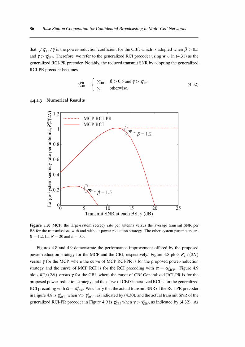
86 Base Station Cooperation for Confidential Broadcasting in Multi-Cell Networks
that√
γ∗CBf/γ is the power-reduction coefficient for the CBf, which is adopted when β > 0.5
and γ > γ∗CBf. Therefore, we refer to the generalized RCI precoder using wPR in (4.31) as the
generalized RCI-PR precoder. Notably, the reduced transmit SNR by adopting the generalized
RCI-PR precoder becomes
γPRCBf =
{γ∗CBf, β > 0.5 and γ > γ∗CBf
γ , otherwise.(4.32)
4.4.2.3 Numerical Results
0 5 10 15 20 250
0.2
0.4
0.6
0.8
1
1.2
= 1.5β
= 1.2β
MCP RCI
MCP RCI-PR
Transmit SNR at each BS, (dB)γ
Rs
Lar
ge-
syst
em s
ecre
cy r
ate
per
an
ten
na,
∞/(
2N
)
Figure 4.8: MCP: the large-system secrecy rate per antenna versus the average transmit SNR perBS for the transmissions with and without power-reduction strategy. The other system parameters areβ = 1.2,1.5,N = 20 and ε = 0.5.
Figures 4.8 and 4.9 demonstrate the performance improvement offered by the proposed
power-reduction strategy for the MCP and the CBf, respectively. Figure 4.8 plots R∞s /(2N)
versus γ for the MCP, where the curve of MCP RCI-PR is for the proposed power-reduction
strategy and the curve of MCP RCI is for the RCI precoding with α = α∗MCP. Figure 4.9
plots R∞s /(2N) versus γ for the CBf, where the curve of CBf Generalized RCI-PR is for the
proposed power-reduction strategy and the curve of CBf Generalized RCI is for the generalized
RCI precoding with α = α∗CBf. We clarify that the actual transmit SNR of the RCI-PR precoder
in Figure 4.8 is γ∗MCP when γ > γ∗MCP, as indicated by (4.30), and the actual transmit SNR of the
generalized RCI-PR precoder in Figure 4.9 is γ∗CBf when γ > γ∗CBf, as indicated by (4.32). As
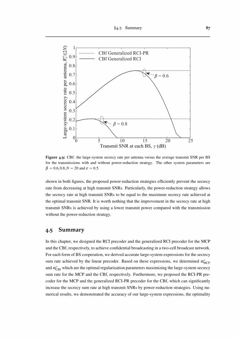
§4.5 Summary 87
0 5 10 15 20 250
0.1
0.2
0.3
0.4
0.5
0.6
0.7
0.8
0.9
1
= 0.8β
= 0.6β
Transmit SNR at each BS, (dB)γ
CBf Generalized RCI
CBf Generalized RCI-PR
Rs
Lar
ge-
syst
em s
ecre
cy r
ate
per
an
ten
na,
∞/(
2N
)
Figure 4.9: CBf: the large-system secrecy rate per antenna versus the average transmit SNR per BSfor the transmissions with and without power-reduction strategy. The other system parameters areβ = 0.6,0.8,N = 20 and ε = 0.5.
shown in both figures, the proposed power-reduction strategies efficiently prevent the secrecy
rate from decreasing at high transmit SNRs. Particularly, the power-reduction strategy allows
the secrecy rate at high transmit SNRs to be equal to the maximum secrecy rate achieved at
the optimal transmit SNR. It is worth nothing that the improvement in the secrecy rate at high
transmit SNRs is achieved by using a lower transmit power compared with the transmission
without the power-reduction strategy.
4.5 Summary
In this chapter, we designed the RCI precoder and the generalized RCI precoder for the MCP
and the CBf, respectively, to achieve confidential broadcasting in a two-cell broadcast network.
For each form of BS cooperation, we derived accurate large-system expressions for the secrecy
sum rate achieved by the linear precoder. Based on these expressions, we determined α∗MCP
and α∗CBf which are the optimal regularization parameters maximizing the large-system secrecy
sum rate for the MCP and the CBf, respectively. Furthermore, we proposed the RCI-PR pre-
coder for the MCP and the generalized RCI-PR precoder for the CBf, which can significantly
increase the secrecy sum rate at high transmit SNRs by power-reduction strategies. Using nu-
merical results, we demonstrated the accuracy of our large-system expressions, the optimality

88 Base Station Cooperation for Confidential Broadcasting in Multi-Cell Networks
of α∗MCP and α∗CBf, and the secrecy sum rate improvement provided by the RCI-PR and the gen-
eralized RCI-PR precoders. Notably, our analytical and numerical results allow us to examine
the impact of the cross-cell interference level on the secrecy sum rate.
Chapter 5
New Secrecy Metrics for WirelessTransmission over Fading Channels
5.1 Introduction
In Chapter 4, we improved the applicability of confidential broadcasting by taking into ac-
count the effects of multi-cell networks. As mentioned earlier in Section 1.2.2, there exists
a fundamental reason that limits the applicability of physical layer security for systems with
practical secrecy requirements. That is, the current definition of secrecy outage probability
has two major limitations in evaluating the secrecy performance of wireless systems: a) the
secrecy outage probability does not give any insight into the eavesdropper’s decodability of
confidential messages; b) the amount of information leakage to the eavesdropper cannot be
characterized.
Motivated by the limitations of the secrecy outage probability, we propose new secrecy
metrics for wireless transmissions focusing on quasi-static fading channels in this chapter.
Different from the secrecy outage probability based on the concept of perfect secrecy, our
proposed secrecy metrics are based on another regime of interest in physical layer security,
namely the partial secrecy regime. The partial secrecy of a system is often investigated by the
equivocation reflecting the level at which the eavesdropper is confused. The exploration on
equivocation can be found as early as Wyner’s pioneering work for the wiretap channel [13].
Similarly, Csiszár and Körner [89] used the normalized equivocation to quantify the partial
secrecy for the broadcast channel with confidential information. Importantly, the equivocation
is closely related to the decoding error probability [13, 90, 91]. Therefore, evaluating the
secrecy performance on the basis of equivocation can reflect the decodability of confidential
messages at the eavesdropper.
It is worth mentioning that the work in this chapter is solely motivated by the limitations
of the current secrecy outage probability from a more practical point of view. Our proposed
new secrecy metrics based on the concept of partial secrecy do not imply that the secrecy met-
rics based on the perfect secrecy is inappropriate from the information-theoretic perspective.
89
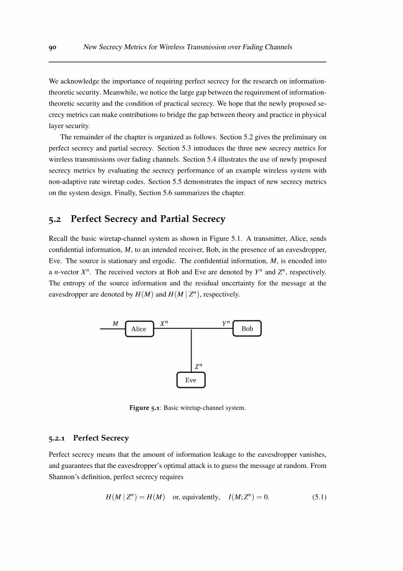
90 New Secrecy Metrics for Wireless Transmission over Fading Channels
We acknowledge the importance of requiring perfect secrecy for the research on information-
theoretic security. Meanwhile, we notice the large gap between the requirement of information-
theoretic security and the condition of practical secrecy. We hope that the newly proposed se-
crecy metrics can make contributions to bridge the gap between theory and practice in physical
layer security.
The remainder of the chapter is organized as follows. Section 5.2 gives the preliminary on
perfect secrecy and partial secrecy. Section 5.3 introduces the three new secrecy metrics for
wireless transmissions over fading channels. Section 5.4 illustrates the use of newly proposed
secrecy metrics by evaluating the secrecy performance of an example wireless system with
non-adaptive rate wiretap codes. Section 5.5 demonstrates the impact of new secrecy metrics
on the system design. Finally, Section 5.6 summarizes the chapter.
5.2 Perfect Secrecy and Partial Secrecy
Recall the basic wiretap-channel system as shown in Figure 5.1. A transmitter, Alice, sends
confidential information, M, to an intended receiver, Bob, in the presence of an eavesdropper,
Eve. The source is stationary and ergodic. The confidential information, M, is encoded into
a n-vector Xn. The received vectors at Bob and Eve are denoted by Y n and Zn, respectively.
The entropy of the source information and the residual uncertainty for the message at the
eavesdropper are denoted by H(M) and H(M | Zn), respectively.
𝑍𝑛
𝑌𝑛 𝑋𝑛 𝑀 Alice Bob
Eve
Figure 5.1: Basic wiretap-channel system.
5.2.1 Perfect Secrecy
Perfect secrecy means that the amount of information leakage to the eavesdropper vanishes,
and guarantees that the eavesdropper’s optimal attack is to guess the message at random. From
Shannon’s definition, perfect secrecy requires
H(M | Zn) = H(M) or, equivalently, I(M;Zn) = 0. (5.1)
§5.2 Perfect Secrecy and Partial Secrecy 91
The requirement of no information leakage to Eve in fact is equivalent to guaranteeing the
highest possible decoding error probability at Eve. As explained in [9, Remark 3.1], consider
that messages are uniformly taken from a size K set [1,2, · · · ,K], and Eve minimizes her de-
coding error probability Pe by performing maximum-likelihood decoding. The condition of no
information leakage ensures that Eve can only guess the original message, and the probability
of error under maximum-likelihood decoding is Pe =K−1
K . Therefore, from the decodability
point of view, perfect secrecy is equivalent to guaranteeing Pe ≥ K−1K . Furthermore, when the
entropy of the message is very large that K → ∞, perfect secrecy actually guarantees that Pe
asymptotically goes to 1,
limK→∞
Pe ≥ limK→∞
K−1K
= 1. (5.2)
In practice, the secrecy requirement on the decodability of messages at Eve can be gener-
ally written as Pe ≥ ϑ for some ϑ . Depending on the applications, the value of ϑ ranges from
0 to 1, which falls outside the perfect secrecy regime.
5.2.2 Partial Secrecy
The partial secrecy is often investigated by the equivocation that indicates the level at which
Eve is confused. We specifically consider the fractional equivocation, which is defined as [15]
∆ =H(M | Zn)
H(M). (5.3)
Note that evaluating security on the basis of equivocation is related to the conventional require-
ment on the decodability of messages at Eve[13]. Although there is no one-to-one relation
between the equivocation and the error probability, the tight lower and upper bounds of the
decoding error probability can be derived from the equivocation [90, 91].
When studying secrecy, we particularly want to ensure that the decoding error probability
at eavesdropper is larger than a certain level. Thus, it is desirable to have the decoding error
probability at Eve lower bounded by the equivocation. Still consider the general case where
messages are uniformly taken from a size K set [1,2, · · · ,K], which achieves the maximal
entropy over an alphabet of size K. Then, the entropy of the message is given by H(M) =
log2(K). From Fano’s inequality [90, Chapter 2.10], we have
H(M | Zn) ≤ h(Pe)+Pe log2(K), (5.4)
where h(x) =−x log2(x)− (1−x) log2(1−x), 0≤ x≤ 1. This inequality can be weakened to
Pe ≥H(M | Zn)−1
log2(K)= ∆− 1
log2(K). (5.5)
92 New Secrecy Metrics for Wireless Transmission over Fading Channels
When the entropy of the message is very large that K→ ∞, we can further derive (5.5) as
limK→∞
Pe ≥ ∆− limK→∞
1log2(K)
= ∆. (5.6)
Thus, Pe is asymptotically lower bounded by ∆.
5.3 New Secrecy Metrics for Wireless Transmissions
Still consider the basic wiretap-channel system. We now assume that the messages are trans-
mitted over quasi-static fading channels. Bob and Eve perfectly know their own CSI. Eve’s
instantaneous CSI is not available at the legitimate side. For wireless transmissions in such a
system, perfect secrecy is not always achievable, and the secrecy outage probability is com-
monly used to measure the secrecy performance. From the perfect secrecy perspective, the
current definition of secrecy outage probability treats the failure of achieving perfect secrecy
as the case of secrecy outage. Thus, the secrecy outage probability is applicable only for
the system which has an extremely stringent requirement on Eve’s decoding error probabil-
ity, ϑ → 1, but cannot handle the general requirement on Eve’s decoding error probability,
0 < ϑ ≤ 1. In addition, the outage-based secrecy metric cannot evaluate how fast or how much
the confidential information is leaked to Eve.
Different from the current secrecy outage probability, we study the secrecy performance
of wireless communications from the partial secrecy perspective. For wireless transmissions
over fading channels, the fractional equivocation, ∆, is a random variable due to the fading
properties of the channel. Thus, we start from the derivation of ∆ for a given fading realization.
The distribution of ∆ can be obtained according to the distribution of channel gains. After that,
three new secrecy metrics are proposed based on the distribution of ∆.
5.3.1 Fractional Equivocation for a Given Fading Realization
A given fading realization of the wireless channel is equivalent to the (non-degraded) Gaussian
wiretap channel[92]. The value of the fractional equivocation for the Gaussian wiretap channel
actually depends on the coding and transmission strategies, and there is no such a general
expression applicable for all scenarios. However, an upper bound on ∆ can be easily derived
following closely from [15, Theorem 1] and [92, Corollary 2]. The maximum achievable
fractional equivocation for a given fading realization of the wireless channel is given by
∆ ≤
1 , if Ce ≤Cb−R
(Cb−Ce)/R , if Cb−R <Ce <Cb
0 , if Cb ≤Ce,
(5.7)
§5.3 New Secrecy Metrics for Wireless Transmissions 93
where Cb and Ce denote Bob and Eve’s channel capacities, respectively, R = H(M)n denotes the
secrecy rate for transmission.
5.3.2 New Secrecy Metrics
From (5.7), we note that the value of ∆ for a given fading realization is determined by the in-
stantaneous channel gains and the transmission rate. Taking into account the fading properties
of wireless channels, we can derive the distribution of ∆ according to the distribution of the
channel gains and the transmission rate. Then, we investigate the distribution of ∆ from three
aspects to propose three secrecy metrics.
5.3.2.1 Generalized Secrecy Outage Probability
Extending the current definition of secrecy outage probability, we propose a generalized defi-
nition of secrecy outage probability, given by
pout = P (∆ < θ ) , (5.8)
where P (·) denotes the probability measure and 0 < θ ≤ 1 denotes the minimum acceptable
value of the fractional equivocation.
Since the fractional equivocation is related to the decoding error probability, the gener-
alized secrecy outage probability is applicable for systems with different levels of secrecy
requirements in terms of Eve’s decodability of confidential messages (by choosing different
values of θ ). The current secrecy outage probability is defined as P (∆ < 1), and hence is a
special case of the newly proposed secrecy outage probability (by setting θ = 1). In the rest of
the chapter, we refer to perfect secrecy outage probability as the current definition of secrecy
outage probability.
Apart from the discussion above, another way to understand the generalized secrecy outage
probability can be described as follows. From (5.3), the information leakage ratio to Eve can
be written as I(M;Zn)H(M)
=1−∆. The information leakage ratio tells the percentage of transmitted
confidential information leaked to the eavesdropper. Then, the generalized secrecy outage
probability, pout = P (∆ < θ ) = P (1−∆ > 1−θ ), actually characterizes the probability that
the information leakage ratio is larger than a certain value, 1−θ .
5.3.2.2 Average Fractional Equivocation
Taking average of the fractional equivocation from its distribution, we can derive the (long-
term) average value of the factional equivocation, given by
∆ = E{∆}, (5.9)
94 New Secrecy Metrics for Wireless Transmission over Fading Channels
where E{·} denotes the expectation operation. As discussed earlier in (5.6), Eve’s decoding
error probability for a given fading realization is asymptotically lower bounded by the frac-
tional equivocation. Thus, the average factional equivocation, ∆, actually gives an asymptotic
lower bound on the overall decoding error probability at Eve, i.e, Pe ≥ ∆.
5.3.2.3 Average Information Leakage Rate
With the knowledge of message transmission rate R = H(M)n , we can further derive the average
information leakage rate, given by
RL = E
{I(M;Zn)
n
}= E
{I(M;Zn)
H(M)· H(M)
n
}= E{(1−∆)R} . (5.10)
The average information leakage rate tells how fast the information is leaked to the eavesdrop-
per. Note that the transmission rate R cannot be simply taken out of the expectation in (5.10),
since R can be a variable parameter (e.g., adaptive rate transmission) and its distribution may
be correlated with the distribution of ∆. However, when the non-adaptive rate transmission
scheme is adopt, (5.10) can be simplified as
RL = E{(1−∆)R}= (1− ∆)R. (5.11)
Remark 5.1. The proposed secrecy metrics in this section, i.e., (5.8), (5.9) and (5.10), are
general and can be applied to evaluate the performance of any coding and transmission strategy
in any system model (e.g., signal-antenna or multi-antenna systems). A specific scenario is
studied as an example in the next section, wherein the expressions for the proposed secrecy
metrics are further derived in terms of transmission rates and channel statistics.
5.4 Wireless Transmissions with Non-Adaptive Rate WiretapCodes: An Example
5.4.1 System Model
We consider the system where a transmitter, Alice, wants to send confidential information to
an intended receiver, Bob, in the present of an eavesdropper, Eve, over quasi-static Rayleigh
fading channels. Alice, Bob and Eve are assumed to have a single antenna each. The instanta-
§5.4 Wireless Transmissions with Non-Adaptive Rate Wiretap Codes: An Example 95
neous channel capacities at Bob and Eve are given by
Cb = log2(1+ γb) (5.12)
and
Ce = log2(1+ γe), (5.13)
respectively, where γb and γe denote the instantaneous received SNRs at Bob and Eve, respec-
tively. The instantaneous received SNRs at Bob and Eve have exponential distributions, given
by
fγb(γb) =1γb
exp(−γb
γb
)(5.14)
and
fγe(γe) =1γe
exp(−γe
γe
), (5.15)
respectively, where γe and γe denote the average received SNRs at Bob and Eve, respectively.
We consider the widely-adopted wiretap code [13] as introduced in Section 1.1.1 for the
message transmissions. The two rate parameters are the codeword transmission rate, Rb, and
the confidential information rate, Rs. We further consider the non-adaptive rate transmission,
where the transmission rates, i.e., Rb and Rs, are fixed over time.
Bob and Eve perfectly know their own channels. Hence, Cb and Ce are known at Bob
and Eve, respectively. Alice has the statistical knowledge on Bob and Eve’s channels, but
does not know either Bob or Eve’s instantaneous CSI. We further assume that Bob provides
a one-bit feedback about his channel quality to Alice in order to avoid unnecessary transmis-
sions [19, 93]. The one-bit feedback enables an on-off transmission scheme to guarantee that
the transmission takes place only when Rb ≤Cb. In addition, the on-off transmission scheme
incurs a probability of transmission, given by
ptx = P (Rb ≤Cb)
= P (Rb ≤ log2(1+ γb))
= exp(−2Rb−1
γb
). (5.16)
5.4.2 Secrecy Performance Evaluation
To characterize the secrecy performance of wireless transmissions over the fading channel, we
start from the investigation on a given fading realization of the channel.
Proposition 5.1. For a given fading realization of the wireless channel, the achievable frac-
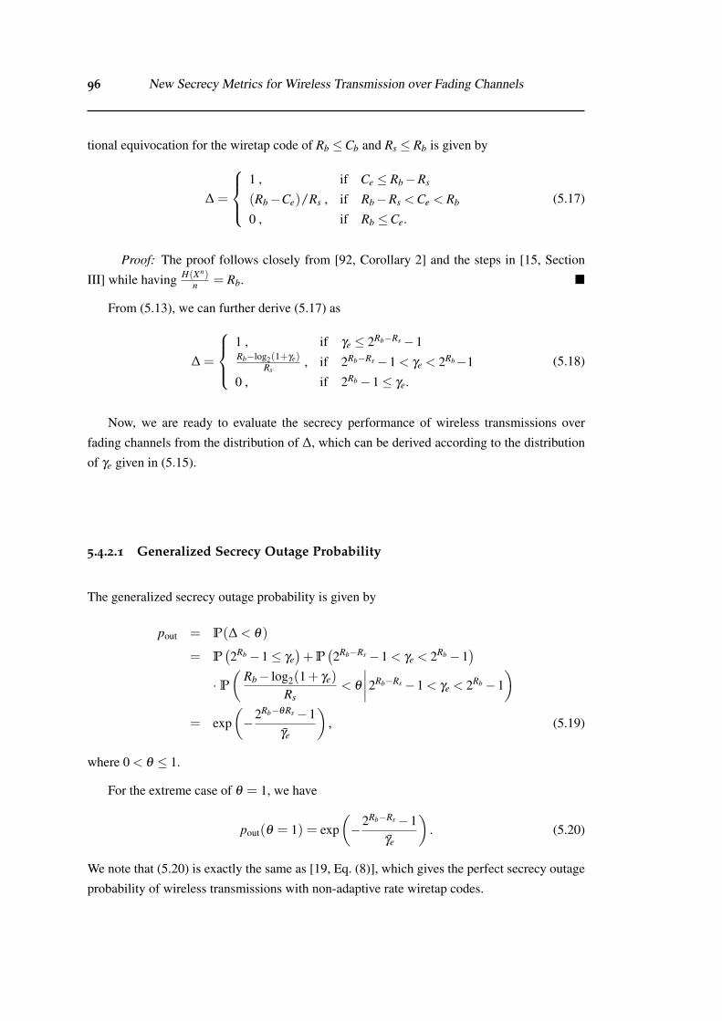
96 New Secrecy Metrics for Wireless Transmission over Fading Channels
tional equivocation for the wiretap code of Rb ≤Cb and Rs ≤ Rb is given by
∆ =
1 , if Ce ≤ Rb−Rs
(Rb−Ce)/Rs , if Rb−Rs <Ce < Rb
0 , if Rb ≤Ce.
(5.17)
Proof: The proof follows closely from [92, Corollary 2] and the steps in [15, Section
III] while having H(Xn)n = Rb. �
From (5.13), we can further derive (5.17) as
∆ =
1 , if γe ≤ 2Rb−Rs−1Rb−log2(1+γe)
Rs, if 2Rb−Rs−1 < γe < 2Rb−1
0 , if 2Rb−1≤ γe.
(5.18)
Now, we are ready to evaluate the secrecy performance of wireless transmissions over
fading channels from the distribution of ∆, which can be derived according to the distribution
of γe given in (5.15).
5.4.2.1 Generalized Secrecy Outage Probability
The generalized secrecy outage probability is given by
pout = P(∆ < θ )
= P(2Rb−1≤ γe
)+P
(2Rb−Rs−1 < γe < 2Rb−1
)· P(
Rb− log2(1+ γe)
Rs< θ
∣∣∣∣2Rb−Rs−1 < γe < 2Rb−1)
= exp(−2Rb−θRs−1
γe
), (5.19)
where 0 < θ ≤ 1.
For the extreme case of θ = 1, we have
pout(θ = 1) = exp(−2Rb−Rs−1
γe
). (5.20)
We note that (5.20) is exactly the same as [19, Eq. (8)], which gives the perfect secrecy outage
probability of wireless transmissions with non-adaptive rate wiretap codes.
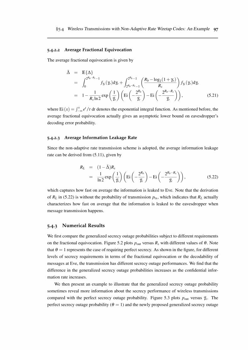
§5.4 Wireless Transmissions with Non-Adaptive Rate Wiretap Codes: An Example 97
5.4.2.2 Average Fractional Equivocation
The average fractional equivocation is given by
∆ = E{∆}
=∫ 2Rb−Rs−1
0fγe(γe)dγe +
∫ 2Rb−1
2Rb−Rs−1
(Rb− log2(1+ γe)
Rs
)fγe(γe)dγe
= 1− 1Rs ln2
exp(
1γe
)(Ei(−2Rb
γe
)−Ei
(−2Rb−Rs
γe
)), (5.21)
where Ei (x) =∫ x−∞
et/t dt denotes the exponential integral function. As mentioned before, the
average fractional equivocation actually gives an asymptotic lower bound on eavesdropper’s
decoding error probability.
5.4.2.3 Average Information Leakage Rate
Since the non-adaptive rate transmission scheme is adopted, the average information leakage
rate can be derived from (5.11), given by
RL = (1− ∆)Rs
=1
ln2exp(
1γe
)(Ei(−2Rb
γe
)−Ei
(−2Rb−Rs
γe
)), (5.22)
which captures how fast on average the information is leaked to Eve. Note that the derivation
of RL in (5.22) is without the probability of transmission ptx, which indicates that RL actually
characterizes how fast on average that the information is leaked to the eavesdropper when
message transmission happens.
5.4.3 Numerical Results
We first compare the generalized secrecy outage probabilities subject to different requirements
on the fractional equivocation. Figure 5.2 plots pout versus Rs with different values of θ . Note
that θ = 1 represents the case of requiring perfect secrecy. As shown in the figure, for different
levels of secrecy requirements in terms of the fractional equivocation or the decodability of
messages at Eve, the transmission has different secrecy outage performances. We find that the
difference in the generalized secrecy outage probabilities increases as the confidential infor-
mation rate increases.
We then present an example to illustrate that the generalized secrecy outage probability
sometimes reveal more information about the secrecy performance of wireless transmissions
compared with the perfect secrecy outage probability. Figure 5.3 plots pout versus γe. The
perfect secrecy outage probability (θ = 1) and the newly proposed generalized secrecy outage
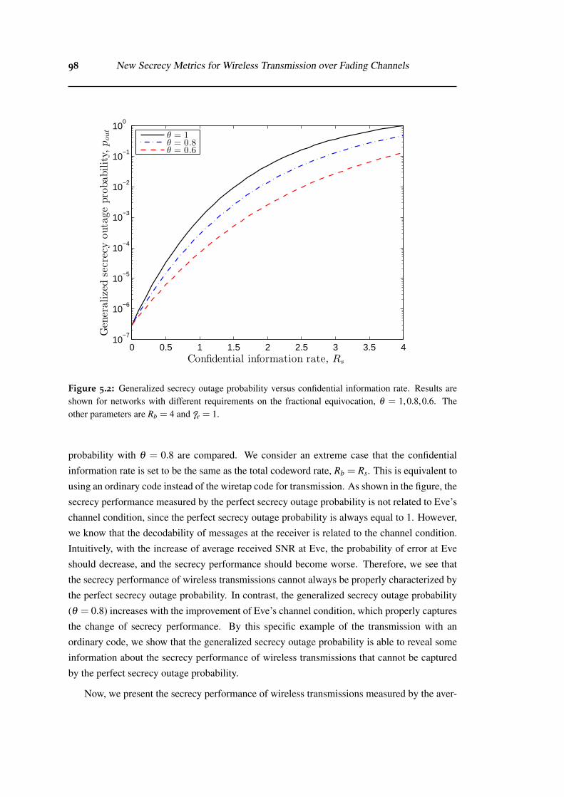
98 New Secrecy Metrics for Wireless Transmission over Fading Channels
0 0.5 1 1.5 2 2.5 3 3.5 410
−7
10−6
10−5
10−4
10−3
10−2
10−1
100
Confidential information rate, Rs
Generalizedsecrecyoutageprobability,
pout
θ = 1θ = 0.8θ = 0.6
Figure 5.2: Generalized secrecy outage probability versus confidential information rate. Results areshown for networks with different requirements on the fractional equivocation, θ = 1,0.8,0.6. Theother parameters are Rb = 4 and γe = 1.
probability with θ = 0.8 are compared. We consider an extreme case that the confidential
information rate is set to be the same as the total codeword rate, Rb = Rs. This is equivalent to
using an ordinary code instead of the wiretap code for transmission. As shown in the figure, the
secrecy performance measured by the perfect secrecy outage probability is not related to Eve’s
channel condition, since the perfect secrecy outage probability is always equal to 1. However,
we know that the decodability of messages at the receiver is related to the channel condition.
Intuitively, with the increase of average received SNR at Eve, the probability of error at Eve
should decrease, and the secrecy performance should become worse. Therefore, we see that
the secrecy performance of wireless transmissions cannot always be properly characterized by
the perfect secrecy outage probability. In contrast, the generalized secrecy outage probability
(θ = 0.8) increases with the improvement of Eve’s channel condition, which properly captures
the change of secrecy performance. By this specific example of the transmission with an
ordinary code, we show that the generalized secrecy outage probability is able to reveal some
information about the secrecy performance of wireless transmissions that cannot be captured
by the perfect secrecy outage probability.
Now, we present the secrecy performance of wireless transmissions measured by the aver-
§5.4 Wireless Transmissions with Non-Adaptive Rate Wiretap Codes: An Example 99
0.5 1 1.5 2 2.5 3
10−0.6
10−0.5
10−0.4
10−0.3
10−0.2
10−0.1
100
Average received SNR at Eve, γe
Generalizedsecrecyoutageprobability,
pout
θ = 1θ = 0.8
Figure 5.3: Generalized secrecy outage probability versus average received SNR at Eve. Results areshown for networks with different requirements on the fractional equivocation, θ = 1,0.8. The otherparameters are Rb = Rs = 4.
age fractional equivocation, which gives an asymptotic lower bound on Eve’s decoding error
probability. Figure 5.4 plots ∆ versus Rs. As shown in the figure, the average fractional equiv-
ocation decreases as the confidential information rate increases and/or the average received
SNR at Eve increases. Besides, we note that even when an ordinary code is used instead of the
wiretap code, i.e., Rb = Rs = 4, Eve still suffers from a relatively high decoding error proba-
bility, e.g., Pe > 0.78 for γe = 1. This observation indicates that the wireless channel itself can
provide a certain level of secrecy for the transmission.
Finally, we illustrate the secrecy performance of wireless transmissions measured by the
average information leakage rate. Figure 5.5 plots RL versus Rs. As the figure shows, the
average information leakage rate increases as the confidential information rate increases and/or
the average received SNR at Eve increases. We note that RL does not reach Rs even when Rs
goes to Rb = 4. This implies that the information is not all leaked to the eavesdropper even
when we use an ordinary code instead of the wiretap code for transmission. This observation
once again confirms that the wireless channel itself can provide a certain level of secrecy for
the transmission.
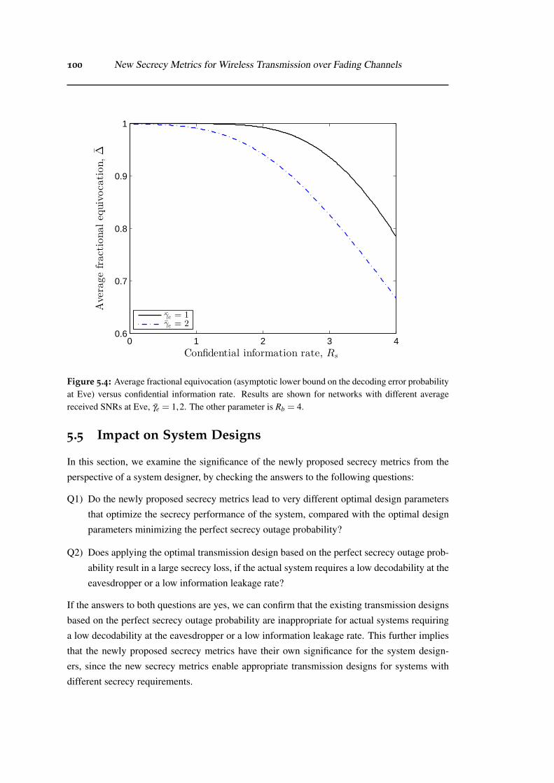
100 New Secrecy Metrics for Wireless Transmission over Fading Channels
0 1 2 3 40.6
0.7
0.8
0.9
1
Confidential information rate, Rs
Averagefractionalequivocation,∆
γe = 1γe = 2
Figure 5.4: Average fractional equivocation (asymptotic lower bound on the decoding error probabilityat Eve) versus confidential information rate. Results are shown for networks with different averagereceived SNRs at Eve, γe = 1,2. The other parameter is Rb = 4.
5.5 Impact on System Designs
In this section, we examine the significance of the newly proposed secrecy metrics from the
perspective of a system designer, by checking the answers to the following questions:
Q1) Do the newly proposed secrecy metrics lead to very different optimal design parameters
that optimize the secrecy performance of the system, compared with the optimal design
parameters minimizing the perfect secrecy outage probability?
Q2) Does applying the optimal transmission design based on the perfect secrecy outage prob-
ability result in a large secrecy loss, if the actual system requires a low decodability at the
eavesdropper or a low information leakage rate?
If the answers to both questions are yes, we can confirm that the existing transmission designs
based on the perfect secrecy outage probability are inappropriate for actual systems requiring
a low decodability at the eavesdropper or a low information leakage rate. This further implies
that the newly proposed secrecy metrics have their own significance for the system design-
ers, since the new secrecy metrics enable appropriate transmission designs for systems with
different secrecy requirements.
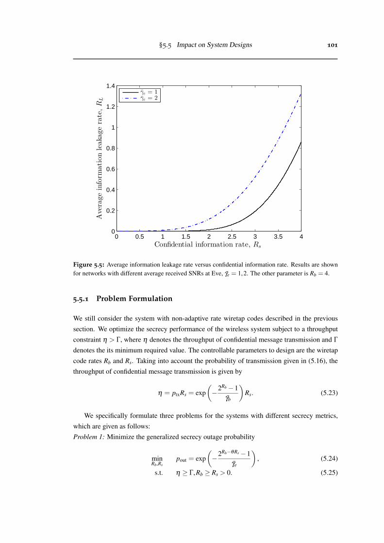
§5.5 Impact on System Designs 101
0 0.5 1 1.5 2 2.5 3 3.5 40
0.2
0.4
0.6
0.8
1
1.2
1.4
Confidential information rate, Rs
Averageinform
ationleakagerate,R
L
γe = 1γe = 2
Figure 5.5: Average information leakage rate versus confidential information rate. Results are shownfor networks with different average received SNRs at Eve, γe = 1,2. The other parameter is Rb = 4.
5.5.1 Problem Formulation
We still consider the system with non-adaptive rate wiretap codes described in the previous
section. We optimize the secrecy performance of the wireless system subject to a throughput
constraint η > Γ, where η denotes the throughput of confidential message transmission and Γdenotes the its minimum required value. The controllable parameters to design are the wiretap
code rates Rb and Rs. Taking into account the probability of transmission given in (5.16), the
throughput of confidential message transmission is given by
η = ptxRs = exp(−2Rb−1
γb
)Rs. (5.23)
We specifically formulate three problems for the systems with different secrecy metrics,
which are given as follows:
Problem 1: Minimize the generalized secrecy outage probability
minRb,Rs
pout = exp(−2Rb−θRs−1
γe
), (5.24)
s.t. η ≥ Γ,Rb ≥ Rs > 0. (5.25)

102 New Secrecy Metrics for Wireless Transmission over Fading Channels
Problem 2: Maximize the average fractional equivocation
maxRb,Rs
∆ = 1− 1Rs ln2
exp(
1γe
)(Ei(−2Rb
γe
)−Ei
(−2Rb−Rs
γe
)), (5.26)
s.t. η ≥ Γ,Rb ≥ Rs > 0. (5.27)
Problem 3: Minimize the average information leakage rate
minRb,Rs
RL =1
ln2exp(
1γe
)(Ei(−2Rb
γe
)−Ei
(−2Rb−Rs
γe
)), (5.28)
s.t. η ≥ Γ,Rb ≥ Rs > 0. (5.29)
5.5.2 Feasibility of the Constraint
The required throughput constraint is not feasible when Γ is larger than the maximum achiev-
able throughput for Rb ≥ Rs > 0. We find that the three problems have the same feasible
constraint region, which is given by the following proposition.
Proposition 5.2. The feasible range of the throughput constraint is given by
0≤ Γ ≤ W0(γb)
ln2exp
(−2
W0(γb)ln2 −1
γb
), (5.30)
where W0(·) denotes the principal branch of the Lambert W function.
Proof: See Appendix D.1. �
5.5.3 Optimal Rate Parameters
We denote Rs,min and Rs,max as the solutions of x to exp(−2x−1
γb
)x = Γ with Rs,min < Rs,max.
The optimal solutions to Problems 1, 2 and 3 are summarized in Propositions 5.3, 5.4 and 5.5,
respectively, as follows.
Proposition 5.3. The optimal rate parameters minimizing the generalized secrecy outage prob-
ability are given as follows:
R∗b1 = log2
(1− γb ln
ΓR∗s1
)(5.31)
and
R∗s1 =
Rs,min , if Rs,min > Rso
Rso , if Rs,min ≤ Rso ≤ Rs,max
Rs,max , if Rs,max < Rso,
(5.32)
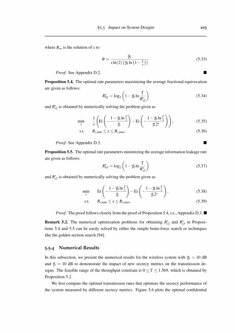
§5.5 Impact on System Designs 103
where Rso is the solution of x to
θ =γb
x ln(2)(γb ln
(1− Γ
x
)) . (5.33)
Proof: See Appendix D.2. �
Proposition 5.4. The optimal rate parameters maximizing the average fractional equivocation
are given as follows:
R∗b2 = log2
(1− γb ln
ΓR∗s2
)(5.34)
and R∗s2 is obtained by numerically solving the problem given as
minx
1x
(Ei
(−
1− γb ln Γx
γe
)−Ei
(−
1− γb ln Γx
γe2x
)), (5.35)
s.t. Rs,min ≤ x≤ Rs,max. (5.36)
Proof: See Appendix D.3. �
Proposition 5.5. The optimal rate parameters minimizing the average information leakage rate
are given as follows:
R∗b3 = log2
(1− γb ln
ΓR∗s3
)(5.37)
and R∗s3 is obtained by numerically solving the problem given as
minx
Ei
(−
1− γb ln Γx
γe
)−Ei
(−
1− γb ln Γx
γe2x
), (5.38)
s.t. Rs,min ≤ x≤ Rs,max. (5.39)
Proof: The proof follows closely from the proof of Proposition 5.4, i.e., Appendix D.3. �
Remark 5.2. The numerical optimization problems for obtaining R∗s2 and R∗s3 in Proposi-
tions 5.4 and 5.5 can be easily solved by either the simple brute-force search or techniques
like the golden section search [94].
5.5.4 Numerical Results
In this subsection, we present the numerical results for the wireless system with γb = 10 dB
and γe = 10 dB to demonstrate the impact of new secrecy metrics on the transmission de-
signs. The feasible range of the throughput constrain is 0 ≤ Γ ≤ 1.569, which is obtained by
Proposition 5.2.
We first compare the optimal transmission rates that optimize the secrecy performance of
the system measured by different secrecy metrics. Figure 5.6 plots the optimal confidential
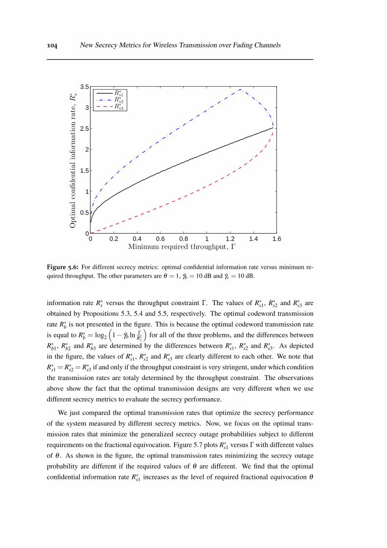
104 New Secrecy Metrics for Wireless Transmission over Fading Channels
0 0.2 0.4 0.6 0.8 1 1.2 1.4 1.60
0.5
1
1.5
2
2.5
3
3.5
Minimum required throughput, Γ
Optimalconfidentialinform
ationrate,R
∗ s
R
∗
s1
R∗
s2
R∗
s3
Figure 5.6: For different secrecy metrics: optimal confidential information rate versus minimum re-quired throughput. The other parameters are θ = 1, γb = 10 dB and γe = 10 dB.
information rate R∗s versus the throughput constraint Γ. The values of R∗s1, R∗s2 and R∗s3 are
obtained by Propositions 5.3, 5.4 and 5.5, respectively. The optimal codeword transmission
rate R∗b is not presented in the figure. This is because the optimal codeword transmission rate
is equal to R∗b = log2
(1− γb ln Γ
R∗s
)for all of the three problems, and the differences between
R∗b1, R∗b2 and R∗b3 are determined by the differences between R∗s1, R∗s2 and R∗s3. As depicted
in the figure, the values of R∗s1, R∗s2 and R∗s3 are clearly different to each other. We note that
R∗s1 = R∗s2 = R∗s3 if and only if the throughput constraint is very stringent, under which condition
the transmission rates are totaly determined by the throughput constraint. The observations
above show the fact that the optimal transmission designs are very different when we use
different secrecy metrics to evaluate the secrecy performance.
We just compared the optimal transmission rates that optimize the secrecy performance
of the system measured by different secrecy metrics. Now, we focus on the optimal trans-
mission rates that minimize the generalized secrecy outage probabilities subject to different
requirements on the fractional equivocation. Figure 5.7 plots R∗s1 versus Γ with different values
of θ . As shown in the figure, the optimal transmission rates minimizing the secrecy outage
probability are different if the required values of θ are different. We find that the optimal
confidential information rate R∗s1 increases as the level of required fractional equivocation θ
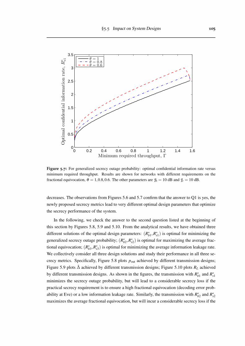
§5.5 Impact on System Designs 105
0 0.2 0.4 0.6 0.8 1 1.2 1.4 1.60
0.5
1
1.5
2
2.5
3
3.5
Minimum required throughput, Γ
Optimalconfidentialinform
ationrate,R
∗ s1
θ = 1θ = 0.8θ = 0.6
Figure 5.7: For generalized secrecy outage probability: optimal confidential information rate versusminimum required throughput. Results are shown for networks with different requirements on thefractional equivocation, θ = 1,0.8,0.6. The other parameters are γb = 10 dB and γe = 10 dB.
decreases. The observations from Figures 5.6 and 5.7 confirm that the answer to Q1 is yes, the
newly proposed secrecy metrics lead to very different optimal design parameters that optimize
the secrecy performance of the system.
In the following, we check the answer to the second question listed at the beginning of
this section by Figures 5.8, 5.9 and 5.10. From the analytical results, we have obtained three
different solutions of the optimal design parameters: (R∗b1,R∗s1) is optimal for minimizing the
generalized secrecy outage probability; (R∗b2,R∗s2) is optimal for maximizing the average frac-
tional equivocation; (R∗b3,R∗s3) is optimal for minimizing the average information leakage rate.
We collectively consider all three design solutions and study their performance in all three se-
crecy metrics. Specifically, Figure 5.8 plots pout achieved by different transmission designs;
Figure 5.9 plots ∆ achieved by different transmission designs; Figure 5.10 plots RL achieved
by different transmission designs. As shown in the figures, the transmission with R∗b1 and R∗s1
minimizes the secrecy outage probability, but will lead to a considerable secrecy loss if the
practical secrecy requirement is to ensure a high fractional equivocation (decoding error prob-
ability at Eve) or a low information leakage rate. Similarly, the transmission with R∗b2 and R∗s2
maximizes the average fractional equivocation, but will incur a considerable secrecy loss if the
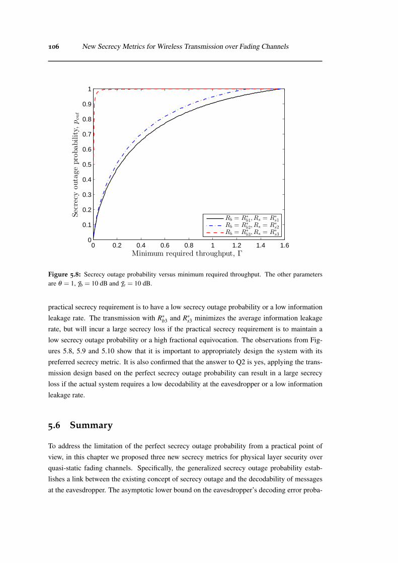
106 New Secrecy Metrics for Wireless Transmission over Fading Channels
0 0.2 0.4 0.6 0.8 1 1.2 1.4 1.60
0.1
0.2
0.3
0.4
0.5
0.6
0.7
0.8
0.9
1
Minimum required throughput, Γ
Secrecyoutageprobability,
pout
Rb = R∗
b1, Rs = R∗
s1
Rb = R∗
b2, Rs = R∗
s2
Rb = R∗
b3, Rs = R∗
s3
Figure 5.8: Secrecy outage probability versus minimum required throughput. The other parametersare θ = 1, γb = 10 dB and γe = 10 dB.
practical secrecy requirement is to have a low secrecy outage probability or a low information
leakage rate. The transmission with R∗b3 and R∗s3 minimizes the average information leakage
rate, but will incur a large secrecy loss if the practical secrecy requirement is to maintain a
low secrecy outage probability or a high fractional equivocation. The observations from Fig-
ures 5.8, 5.9 and 5.10 show that it is important to appropriately design the system with its
preferred secrecy metric. It is also confirmed that the answer to Q2 is yes, applying the trans-
mission design based on the perfect secrecy outage probability can result in a large secrecy
loss if the actual system requires a low decodability at the eavesdropper or a low information
leakage rate.
5.6 Summary
To address the limitation of the perfect secrecy outage probability from a practical point of
view, in this chapter we proposed three new secrecy metrics for physical layer security over
quasi-static fading channels. Specifically, the generalized secrecy outage probability estab-
lishes a link between the existing concept of secrecy outage and the decodability of messages
at the eavesdropper. The asymptotic lower bound on the eavesdropper’s decoding error proba-
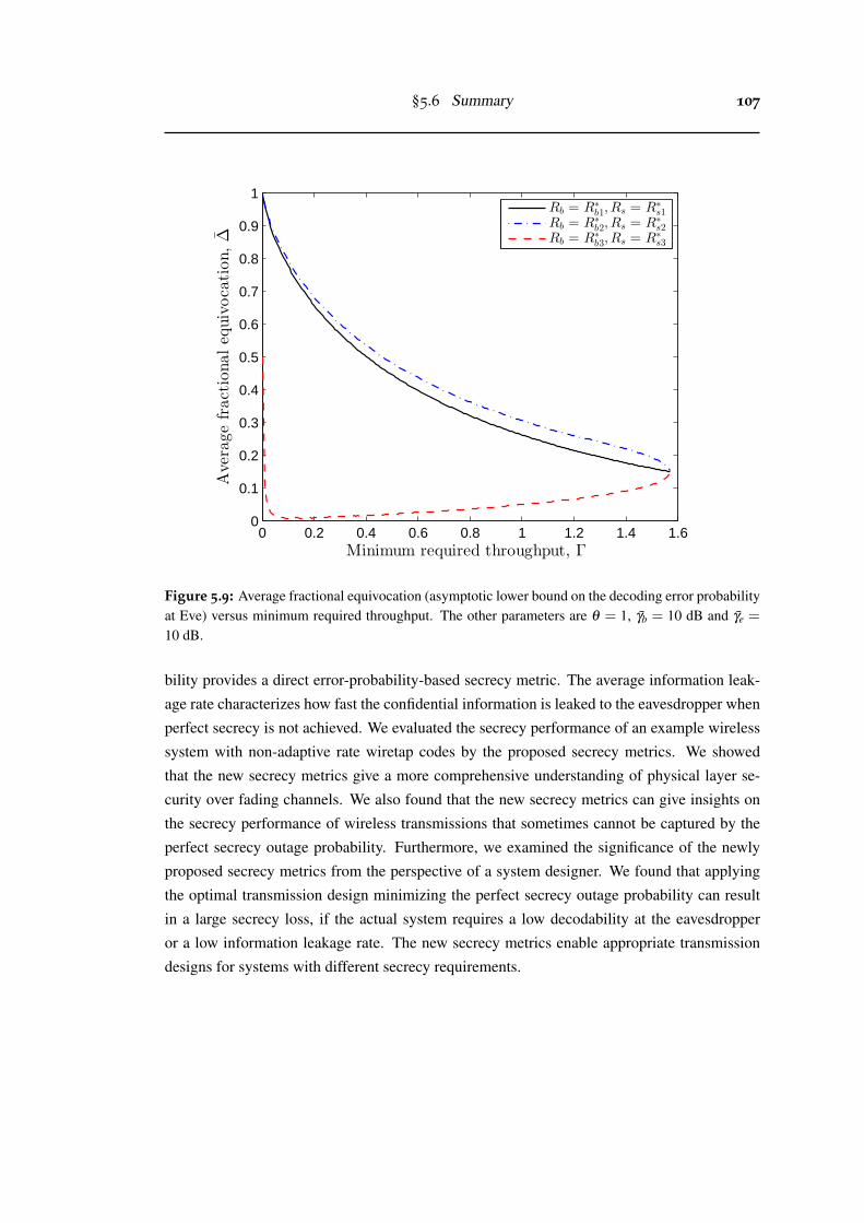
§5.6 Summary 107
0 0.2 0.4 0.6 0.8 1 1.2 1.4 1.60
0.1
0.2
0.3
0.4
0.5
0.6
0.7
0.8
0.9
1
Minimum required throughput, Γ
Averagefractionalequivocation,∆
Rb = R∗
b1, Rs = R∗
s1
Rb = R∗
b2, Rs = R∗
s2
Rb = R∗
b3, Rs = R∗
s3
Figure 5.9: Average fractional equivocation (asymptotic lower bound on the decoding error probabilityat Eve) versus minimum required throughput. The other parameters are θ = 1, γb = 10 dB and γe =
10 dB.
bility provides a direct error-probability-based secrecy metric. The average information leak-
age rate characterizes how fast the confidential information is leaked to the eavesdropper when
perfect secrecy is not achieved. We evaluated the secrecy performance of an example wireless
system with non-adaptive rate wiretap codes by the proposed secrecy metrics. We showed
that the new secrecy metrics give a more comprehensive understanding of physical layer se-
curity over fading channels. We also found that the new secrecy metrics can give insights on
the secrecy performance of wireless transmissions that sometimes cannot be captured by the
perfect secrecy outage probability. Furthermore, we examined the significance of the newly
proposed secrecy metrics from the perspective of a system designer. We found that applying
the optimal transmission design minimizing the perfect secrecy outage probability can result
in a large secrecy loss, if the actual system requires a low decodability at the eavesdropper
or a low information leakage rate. The new secrecy metrics enable appropriate transmission
designs for systems with different secrecy requirements.
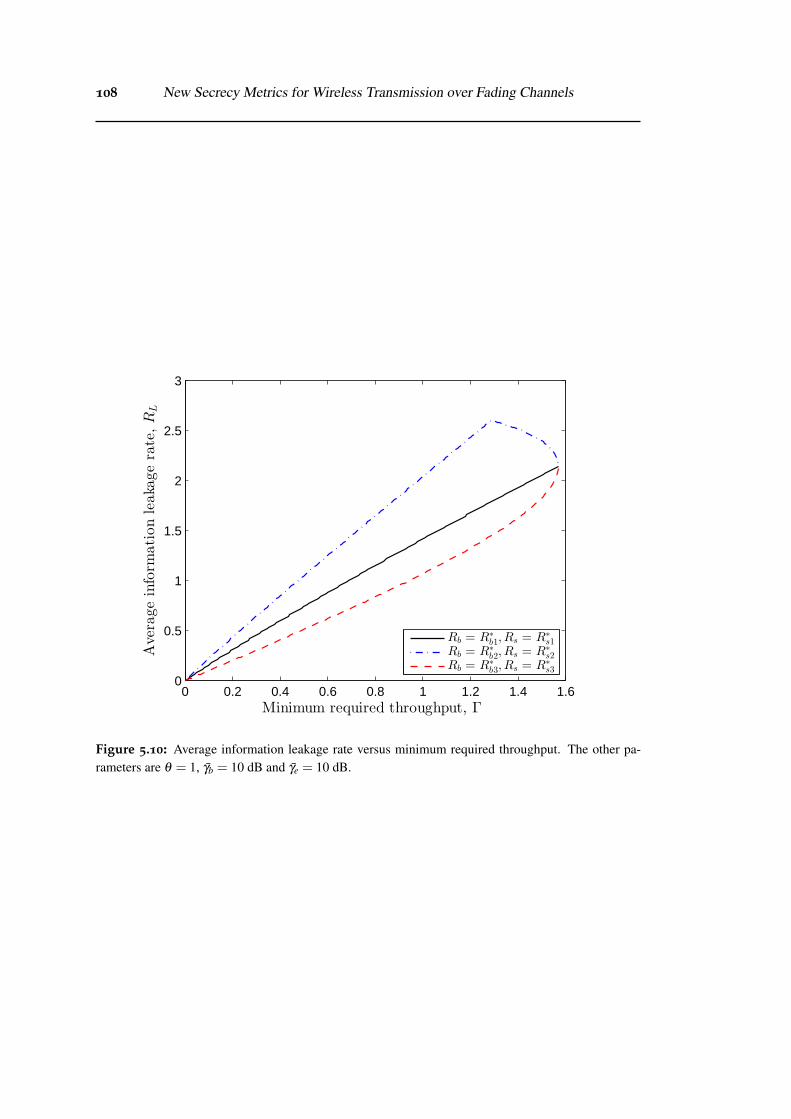
108 New Secrecy Metrics for Wireless Transmission over Fading Channels
0 0.2 0.4 0.6 0.8 1 1.2 1.4 1.60
0.5
1
1.5
2
2.5
3
Minimum required throughput, Γ
Averageinform
ationleakagerate,R
L
Rb = R∗
b1, Rs = R∗
s1
Rb = R∗
b2, Rs = R∗
s2
Rb = R∗
b3, Rs = R∗
s3
Figure 5.10: Average information leakage rate versus minimum required throughput. The other pa-rameters are θ = 1, γb = 10 dB and γe = 10 dB.
Chapter 6
Conclusions
In this chapter, we first summarize the general conclusions drawn from the thesis, and then
outline some future research directions.
6.1 Thesis Conclusions
Motivated by the large gap between theory and practice in wireless physical layer security,
this thesis has studied the wireless physical layer security towards practical assumptions and
requirements.
In the first half of the thesis, we reduced the dependence of physical layer security on im-
practical assumptions. We first studied the secure transmission designs with the consideration
of channel estimation errors, against the impractical assumption of perfect CSI. We presented a
comprehensive study of secure on-off transmission design with different transmission schemes,
i.e., the fixed rate transmission, the non-adaptive rate transmission, and the adaptive rate trans-
mission. Our results illustrated how the optimal design and the achievable system performance
vary with the change in the channel knowledge assumptions. We then introduced the spa-
tial constraint into physical layer security, which provides an innovative approach to study
the multi-antenna secure networks without the impractical assumption of knowing the number
of eavesdropper antennas. With the spatial constraints at the receiver side, we investigated
the wiretap-channel system, the basic jammer-assisted system, and the AN jammer-assisted
system. We found that a non-zero secrecy capacity is achievable with the assist of jamming
signals, even if the eavesdropper is equipped with infinite number of antennas.
In the second half of the thesis, we improved the applicability of the study on physical
layer security. Firstly, we designed linear precoders to achieve confidential broadcasting in a
two-cell broadcast network, while the current confidential broadcasting is applicable only in
single-cell networks. We considered two forms of BS cooperation, i.e., the MCP and the CBf.
For each form of BS cooperation, we proposed an appropriate linear precoder to efficiently
achieve the confidential broadcasting. We conducted the large-system analysis, and optimized
the precoder designs based on the large-system results. Secondly, we proposed new secrecy
109
110 Conclusions
metrics for physical layer security over fading channels. This is motivated by the limitations
of the perfect secrecy outage probability on evaluating wireless systems with practical require-
ments. The newly proposed secrecy metrics can give insights on the secrecy performance of
wireless transmissions that sometimes cannot be captured by the perfect secrecy outage proba-
bility. Our results showed that the new secrecy metrics enable appropriate transmission designs
for systems with practical secrecy requirements.
6.2 Future Research Directions
In this section, we point out some possible future research directions that arise from the work
presented in this thesis.
Secure communications with spatial constraints at the transmitter and the receiver:As a first step of studying the effects of spatial constraints on physical layer security, Chap-
ter 3 considered a simple scenario with spatial constraints at the receiver side only. A natural
future work is to extend the study by investigating the effects of spatial constraints at both the
transmitter and the receiver sides. To this end, a limited number of transmit antennas with the
spatial constraint at the transmitter should be considered [95]. However, it is worth mention-
ing that the extension is non-trivial, since the secrecy capacity would depend on instantaneous
channel realizations even if the number of transmit antennas goes to infinity.
Stochastic geometry in broadcast networks with confidential information: Chapter 4
assumed a simple homogenous scenario where the users in the same cell are located at the
same distance away from the BS. In practical networks, the users are more likely to spatially
randomly distributed in the network with different distances to the BS. To characterize the ran-
domness of user locations, we can adopt the stochastic geometry approach [96] for modeling
the user locations, since it allows us to appropriately study the probabilistic network behav-
iors and corresponding performance metrics [97, 98, 99, 100]. In fact, the spatial modeling of
user locations using stochastic geometry approach has already been adopted in the research of
physical layer security, e.g., [101, 102, 103], while it has never been considered in the study of
confidential broadcasting.
Analysis and design of physical layer security based on the new secrecy metrics: In
Chapter 5, we proposed new secrecy metrics for wireless transmission over fading channels. A
natural future research direction is to adopt the proposed secrecy metrics to analyze physical
layer security in wireless systems. Also, it is interesting to develop efficient secure transmission
designs or secrecy enhancements based on the proposed secrecy metrics, according to the
secrecy requirements on practical wireless networks.
Appendix A
Appendix A
A.1 Proof of Proposition 2.1
We first derive the optimal µb in Scenario 1. One can find that µb = 2Rb−1 is the only solution
of µb to the equation∂η(µb, µe)
∂ µb= 0 (A.1)
and∂ 2η(2Rb−1, µe)
∂ µ2b
< 0. (A.2)
Thus, if we ignore the possible bound of µb, the optimal µb is equal to 2Rb − 1. However, to
satisfy the reliability constraint, pco ≤ δ , there exists a possible lower bound of µb given by
µb ≥(2Rb−1
)(1−αbςb ln
(δ
1+ ςb(2Rb−2)ςb(2Rb−1)
)). (A.3)
Considering the lower bound, the optimal µb in Scenario 1 is formulated as (2.27) in Proposi-
tion 2.1.
Then, we derive the optimal µe in Scenario 1. Since ptx is an increasing function of µe and
pco is independent of µe, it is optimal to maximize µe while satisfying the security constraint
pso ≤ ϕ . From the definition of pso, one can find that pso is an increasing function of µe. Thus,
there is only one or no solution of µe to the equation
pso(µe) = ϕ , (A.4)
where the expression of pso is given as (2.23). When
Pr(Ce > Rb−Rs) ≤ ϕ ⇔ 1− ςe
1+ ςe(2Rb−Rs−2)exp(− 2Rb−Rs−1
αe(1− ςe)
)≤ ϕ , (A.5)
there is no solution of µe to (A.4), which means that there is no need to set an on-off SNR
threshold on γe for the system (the required security constraint is always achievable) or equiv-
111
112 Appendix A
alently µe = ∞. Otherwise, there exists one and only one solution of µe to (A.4), which is
the optimal value of µe to the maximization problem. The optimal µe in Scenario 1 can be
numerically solved as given in (2.28). This completes the proof of Proposition 2.1.
A.2 Proof of Proposition 2.2
The optimal µb in Scenario 2 is the same as that in Scenario 1 and the proof of it is identical
to the corresponding part in the proof of Proposition 2.1. Now, we derive the optimal µe in
Scenario 2. Since ptx is an increasing function of µe and pco is independent of µe, it is optimal
to maximize µe while satisfying the security constraint pso ≤ ϕ . From the definition of pso,
one can find that pso is an increasing function of µe. Thus, there is only one or no solution of
µe to the equation
pso(µe) = ϕ , (A.6)
where the expression of pso is given as (2.34). When
Pr(Ce > Rb−Rs) ≤ ϕ ⇔ exp(−2Rb−Rs−1
αe
)≤ ϕ , (A.7)
there is no solution of µe to (A.6), which means that there is no need to set an on-off SNR
threshold on γe for the system (the required security constraint is always achievable) or equiv-
alently µe = ∞. Otherwise, there exists one and only one solution of µe to (A.6), which is
the optimal value of µe to the maximization problem. The optimal µe in Scenario 2 can be
numerically solved as given in (2.38). This completes the proof of Proposition 2.2.
A.3 Proof of Proposition 2.4
The proof of the optimal µb for the non-adaptive scheme is identical to the proof of optimal
µb in Section 2.3. Now, we prove the optimal Rs for any chosen Rb as follows. Since ptx and
pco are independent of Rs, it is optimal to maximize Rs. Thus, we obtain the optimal Rs while
satisfying pso ≤ ϕ as (2.57) in Proposition 2.4. Then, we prove the optimal Rb. Since Rs > 0,
we have Rb > k. It is easy to prove that when
Rb ≥max{
log2
(1+
(1− ςb)δ
ςb(1−δ )
),k+
1ln2
W0
(2−k
αb(1− ςb))}
, (A.8)
the value of η is a decreasing function of Rb, i.e,
∂η(µb,Rb)
∂Rb< 0. (A.9)
§A.4 Proof of Proposition 2.5 113
Therefore, the optimal Rb can be obtained by solving the optimization problem given in Propo-
sition 2.4. This completes to proof of Proposition 2.4.
A.4 Proof of Proposition 2.5
The proof of the optimal Rs for the adaptive rate scheme is identical to the corresponding part
in the proof of Proposition 2.4. Now, we derive the optimal Rb. To satisfy Rs > 0 and pco ≤ δ ,
we obtain the lower and upper bounds of Rb given by Rb > k and Rb ≤ log2
(1+ γb
1+αbςb lnδ−1
).
Thus, the optimal Rb can be obtained by solving the optimization problem given in Proposi-
tion 2.5. Then, we derive the optimal µb. To derive the optimal, µb, we start from looking for
the range of γb in which it is possible to have secure communication with positive confidential
information rate while satisfying both constraints. Let the lower bound of Rb be less than the
upper bound of Rb, we can find the feasible range of γb as
log2(1+αe ln
(ϕ−1))< log2
(1+
γb
1+αbςb lnδ−1
)⇔ γb >
(1+αbςb lnδ
−1)αe ln
(ϕ−1) .
(A.10)
Therefore, the optimal µb is equal to the lower bound of the feasible γb, given by (2.65). This
completes to proof of Proposition 2.5.

114 Appendix A
Appendix B
Appendix B
B.1 Proof of Proposition 3.1
The capacity of Bob or Eve’s channel can be written as
Ci = log∣∣∣∣INi +
αiHiQxHHi
σ2i
∣∣∣∣ , (B.1)
where Qx denotes the covariance matrix of x, i.e., Qx = E{
xxH}
. Since Alice has no instan-
taneous CSI of Bob and there is sufficient space at Alice for independent transmit antenna
allocation, the best transmission strategy is to have the transmit signal vector composed of sta-
tistically independent equal power components, each with a Gaussian distribution. Then, the
covariance matrix of x is equal to Qx =PtNt
INt , and the channel capacity becomes to
Ci = log∣∣∣∣INi +
αiPt
σ2i Nt
HiHHi
∣∣∣∣ , (B.2)
where
HiHHi =
Nt
∑t=1
hithHit . (B.3)
Considering a large number of transmit antennas (Nt → ∞) and sufficient space for placing
transmit antennas (independent hit), the correlation matrix at the receiver in (3.2) becomes to
Ri→1Nt
Nt
∑t=1
hithHit . (B.4)
Note that there is no expectation over channel realizations in (B.4), since 1Nt
∑Ntt=1 hithH
it =
E{
1Nt
∑Ntt=1 hithH
it
}when Nt → ∞. Then, the channel capacity with a large number of suffi-
ciently separated transmit antennas is approximated by
Ci ≈ log∣∣∣∣INi +
αiPt
σ2i
Ri
∣∣∣∣ . (B.5)
115
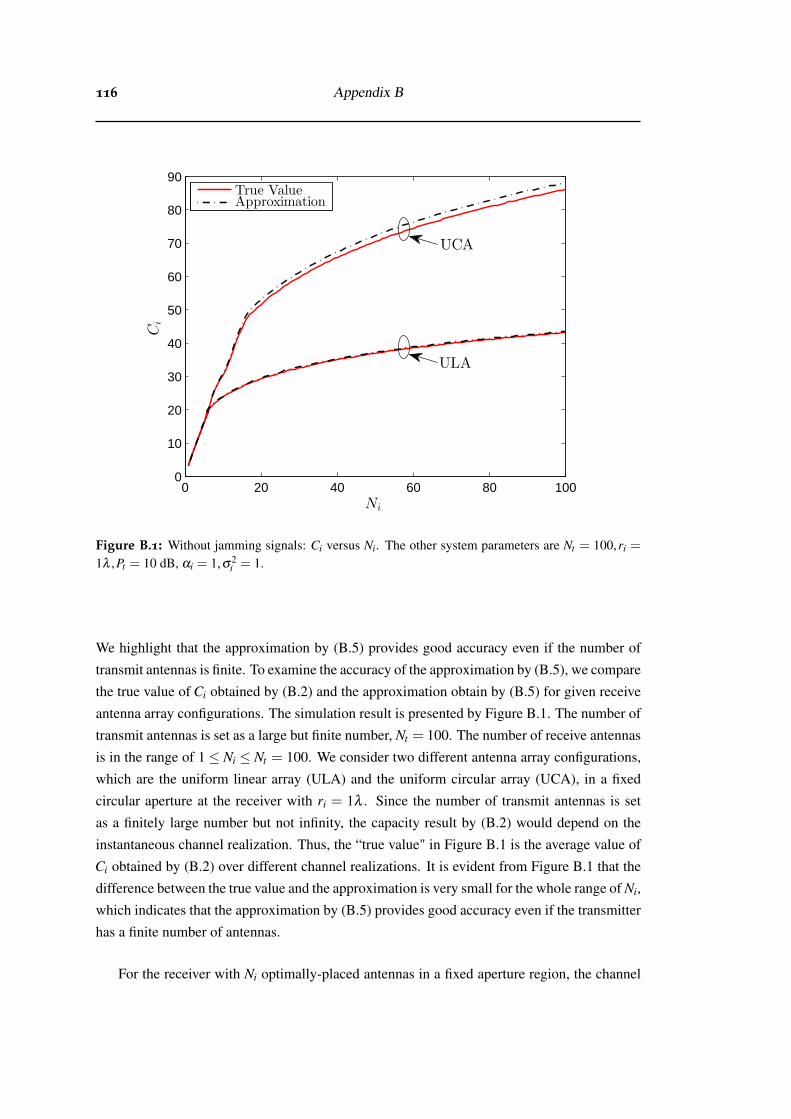
116 Appendix B
0 20 40 60 80 1000
10
20
30
40
50
60
70
80
90
ULA
UCA
Ni
Ci
True ValueApproximation
Figure B.1: Without jamming signals: Ci versus Ni. The other system parameters are Nt = 100,ri =
1λ ,Pt = 10 dB, αi = 1,σ2i = 1.
We highlight that the approximation by (B.5) provides good accuracy even if the number of
transmit antennas is finite. To examine the accuracy of the approximation by (B.5), we compare
the true value of Ci obtained by (B.2) and the approximation obtain by (B.5) for given receive
antenna array configurations. The simulation result is presented by Figure B.1. The number of
transmit antennas is set as a large but finite number, Nt = 100. The number of receive antennas
is in the range of 1≤ Ni ≤ Nt = 100. We consider two different antenna array configurations,
which are the uniform linear array (ULA) and the uniform circular array (UCA), in a fixed
circular aperture at the receiver with ri = 1λ . Since the number of transmit antennas is set
as a finitely large number but not infinity, the capacity result by (B.2) would depend on the
instantaneous channel realization. Thus, the “true value" in Figure B.1 is the average value of
Ci obtained by (B.2) over different channel realizations. It is evident from Figure B.1 that the
difference between the true value and the approximation is very small for the whole range of Ni,
which indicates that the approximation by (B.5) provides good accuracy even if the transmitter
has a finite number of antennas.
For the receiver with Ni optimally-placed antennas in a fixed aperture region, the channel
§B.2 Proof of Theorem 3.1 117
capacity in (B.5) can be further approximated by [70, Chapter 3],
Ci ≈
Ni log(1+ αiPtσ2
i) , if Ni ≤ N0i
N0i log(1+ NiN0i
αiPtσ2
i) , if Ni > N0i,
(B.6)
where the expression of N0i for a 2D circular aperture or a 3D spherical aperture is given
by (3.9). The Ci in (B.6) is derived with the approximation that Jm(2π
λri)→ 0 for m ≥
dπeri/λe+ 1, where Jm(·) denotes the Bessel function of order m. Such an approximation
is shown to be very accurate in [70].
Finally, substituting (B.6) into (3.8) completes the proof of Proposition 3.1.
B.2 Proof of Theorem 3.1
The capacity of Bob or Eve’s channel subject to the basic jamming signals is written as [104,
Section 3.1]
Ci = log∣∣∣INi +αiHiQxHH
i(βiGiQwGH
i +σ2i INi
)−1∣∣∣ , (B.7)
where Qx and Qw denote the covariance matrices of x and w1, respectively, i.e., Qx = E{
xxH}
and Qw = E{
w1wH1}
. Since neither Alice nor Helen has the instantaneous CSI to Bob or Eve,
the equal power allocation at the transmit antennas is adopted at both Alice and Helen, and the
covariance matrices of x and w1 are equal to Qx =PtNt
INt and Qw =PjN j
IN j , respectively. Then,
the channel capacity becomes to
Ci = log
∣∣∣∣∣INi +αiPt
NtHiHH
i
(βiPj
N jGiGH
i +σ2i INi
)−1∣∣∣∣∣ . (B.8)
Considering the large number of transmit antennas (Nt → ∞,N j → ∞) and sufficient space for
placing transmit antennas (independent hit and independent git), we have
1Nt
Nt
∑t=1
hithHit =
1N j
N j
∑t=1
gitgHit = Ri, (B.9)
where Ri is the correlation matrix at the receiver side. Note that Ri is determined by the receive
antenna correlations.

118 Appendix B
Therefore, the channel capacity can be approximated by
Ci ≈ log∣∣∣INi +αiPtRi
(βiPjRi +σ
2i INi
)−1∣∣∣
= log∣∣∣(αiPtRi +βiPjRi +σ
2i INi
)(βiPjRi +σ
2i INi
)−1∣∣∣
= log
∣∣∣∣∣(
INi +
(αiPt
σ2i
+βiPj
σ2i
)Ri
)(INi +
βiPj
σ2i
Ri
)−1∣∣∣∣∣
= log∣∣∣∣INi +
(αiPt
σ2i+
βiPj
σ2i
)Ri
∣∣∣∣− log∣∣∣∣INi +
βiPj
σ2i
Ri
∣∣∣∣ . (B.10)
We highlight that the approximation by (B.10) provides good accuracy even if the number of
transmit antennas and the number of jamming antennas are finite. To examine the accuracy
of the approximation by (B.10), we compare the true value of Ci obtained by (B.8) and the
approximation obtain by (B.10) for given receive antenna array configurations. The simulation
result is presented by Figure B.2. The number of transmit antennas and the number of jamming
antennas are set as Nt = N j = 100. The number of receive antennas is in the range of 1≤ Ni ≤Nt = N j = 100. We still consider two different antenna array configurations, i.e., the ULA and
the UCA, in a fixed circular aperture at the receiver with ri = 1λ . It is evident from Figure B.2
that the difference between the true value and the approximation is very small for the whole
range of Ni. This confirms that the approximation by (B.10) provides good accuracy even if
the transmitter and the jammer have finite numbers of antennas.
For the receiver with Ni optimally-placed antennas in a fixed aperture region, the channel
capacity in (B.10) can be further approximated by
Ci ≈
Ni log(
1+ αiPtσ2
i+
βiPj
σ2i
)−Ni log
(1+ βiPj
σ2i
), if Ni ≤ N0i
N0i log(
1+ NiN0i
(αiPtσ2
i+
βiPj
σ2i
))−N0i log
(1+ Ni
N0i
βiPj
σ2i
), if Ni > N0i
=
Ni log
(1+ αiPt
βiPj+σ2i
), if Ni ≤ N0i
N0i log(
1+NiN0i
αiPtNiN0i
βiPj+σ2i
), if Ni > N0i.
(B.11)
Still, the Ci in (B.11) is derived with the approximation that Jm(2π
λri)→ 0 for m≥ dπeri/λe+
1.
Finally, substituting (B.11) into (3.8) completes the proof of Theorem 3.1.
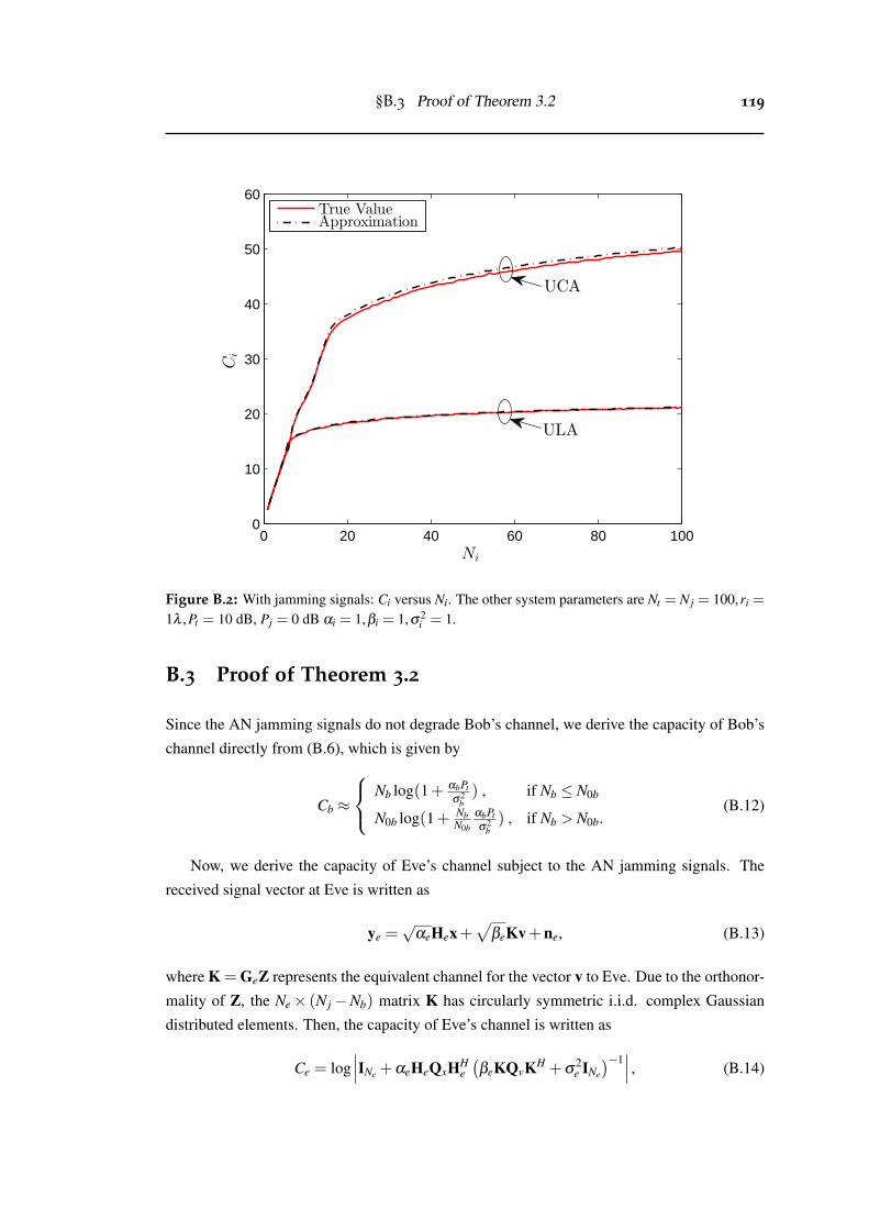
§B.3 Proof of Theorem 3.2 119
0 20 40 60 80 1000
10
20
30
40
50
60
ULA
UCA
Ni
Ci
True ValueApproximation
Figure B.2: With jamming signals: Ci versus Ni. The other system parameters are Nt = N j = 100,ri =
1λ ,Pt = 10 dB, Pj = 0 dB αi = 1,βi = 1,σ2i = 1.
B.3 Proof of Theorem 3.2
Since the AN jamming signals do not degrade Bob’s channel, we derive the capacity of Bob’s
channel directly from (B.6), which is given by
Cb ≈
Nb log(1+ αbPtσ2
b) , if Nb ≤ N0b
N0b log(1+ NbN0b
αbPtσ2
b) , if Nb > N0b.
(B.12)
Now, we derive the capacity of Eve’s channel subject to the AN jamming signals. The
received signal vector at Eve is written as
ye =√
αeHex+√
βeKv+ne, (B.13)
where K = GeZ represents the equivalent channel for the vector v to Eve. Due to the orthonor-
mality of Z, the Ne× (N j−Nb) matrix K has circularly symmetric i.i.d. complex Gaussian
distributed elements. Then, the capacity of Eve’s channel is written as
Ce = log∣∣∣INe +αeHeQxHH
e(βeKQvKH +σ
2e INe
)−1∣∣∣ , (B.14)
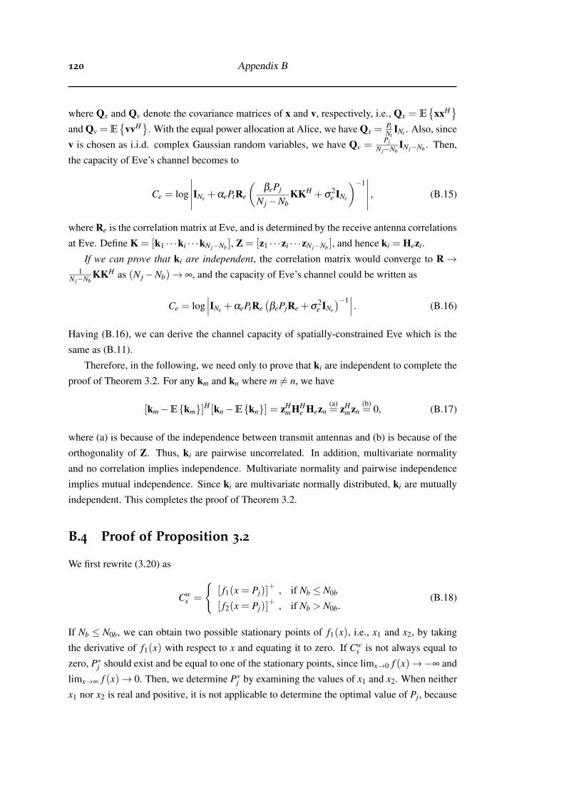
120 Appendix B
where Qx and Qv denote the covariance matrices of x and v, respectively, i.e., Qx = E{
xxH}
and Qv = E{
vvH}
. With the equal power allocation at Alice, we have Qx =PtNt
INt . Also, since
v is chosen as i.i.d. complex Gaussian random variables, we have Qv =Pj
N j−NbIN j−Nb . Then,
the capacity of Eve’s channel becomes to
Ce = log
∣∣∣∣∣INe +αePtRe
(βePj
N j−NbKKH +σ
2e INe
)−1∣∣∣∣∣ , (B.15)
where Re is the correlation matrix at Eve, and is determined by the receive antenna correlations
at Eve. Define K = [k1 · · ·ki · · ·kN j−Nb ], Z = [z1 · · ·zi · · ·zN j−Nb ], and hence ki = Hezi.
If we can prove that ki are independent, the correlation matrix would converge to R→1
N j−NbKKH as (N j−Nb)→ ∞, and the capacity of Eve’s channel could be written as
Ce = log∣∣∣INe +αePtRe
(βePjRe +σ
2e INe
)−1∣∣∣ . (B.16)
Having (B.16), we can derive the channel capacity of spatially-constrained Eve which is the
same as (B.11).
Therefore, in the following, we need only to prove that ki are independent to complete the
proof of Theorem 3.2. For any km and kn where m 6= n, we have
[km−E{km}]H [kn−E{kn}] = zHmHH
e Hezn(a)= zH
mzn(b)= 0, (B.17)
where (a) is because of the independence between transmit antennas and (b) is because of the
orthogonality of Z. Thus, ki are pairwise uncorrelated. In addition, multivariate normality
and no correlation implies independence. Multivariate normality and pairwise independence
implies mutual independence. Since ki are multivariate normally distributed, ki are mutually
independent. This completes the proof of Theorem 3.2.
B.4 Proof of Proposition 3.2
We first rewrite (3.20) as
Cws =
{[ f1(x = Pj)]
+ , if Nb ≤ N0b
[ f2(x = Pj)]+ , if Nb > N0b.
(B.18)
If Nb ≤ N0b, we can obtain two possible stationary points of f1(x), i.e., x1 and x2, by taking
the derivative of f1(x) with respect to x and equating it to zero. If Cws is not always equal to
zero, P∗j should exist and be equal to one of the stationary points, since limx→0 f (x)→−∞ and
limx→∞ f (x)→ 0. Then, we determine P∗j by examining the values of x1 and x2. When neither
x1 nor x2 is real and positive, it is not applicable to determine the optimal value of Pj, because
§B.4 Proof of Proposition 3.2 121
the stationary point for f1(x) does not exist, and Cws is always equal to zero for any value of Pj.
Similarly, if Nb > N0b, we can obtain two possible stationary points of f2(x), i.e., x3 and x4,
by taking the derivative of f2(x) with respect to x and equating it to zero. Then, we determine
P∗j by examining the values of x3 and x4. When neither x3 nor x4 is real and positive, it is not
applicable to determine the optimal value of Pj, because Cws is always equal to zero for any
value of Pj. This completes the proof of Proposition 3.2.

122 Appendix B

Appendix C
Appendix C
C.1 Proof of Theorem 4.1
We first derive the large-system approximations of the SINRs for message sk, j at the intended
receiver and the eavesdropper. Based on the approximations, we then obtain the large-system
secrecy sum rate using (4.22).
We recall that the following equality holds:
(HHH+αI2N
)−1=(
HHk, jHk, j +hH
k, jhk, j +αI2N
)−1. (C.1)
By applying the matrix inversion lemma, we obtain
(HHH+αI2N
)−1=(
HHk, jHk, j +αI2N
)−1
−
(HH
k, jHk, j +αI2N
)−1hH
k, jhk, j
(HH
k, jHk, j +αI2N
)−1
1+hk, j
(HH
k, jHk, j +αI2N
)−1hH
k, j
. (C.2)
Then let us define
Zk, j = Ok, j−Ok, j
(1N hH
k, jhk, j
)Ok, j
1+ 1N hk, jOk, jhH
k, j
, (C.3)
where
Ok, j =
(1N
HHk, jHk, j +
α
NI2N
)−1
. (C.4)
This allows us to rewrite (C.2) as
(HHH+αI2N
)−1=
1N
Zk, j. (C.5)
123
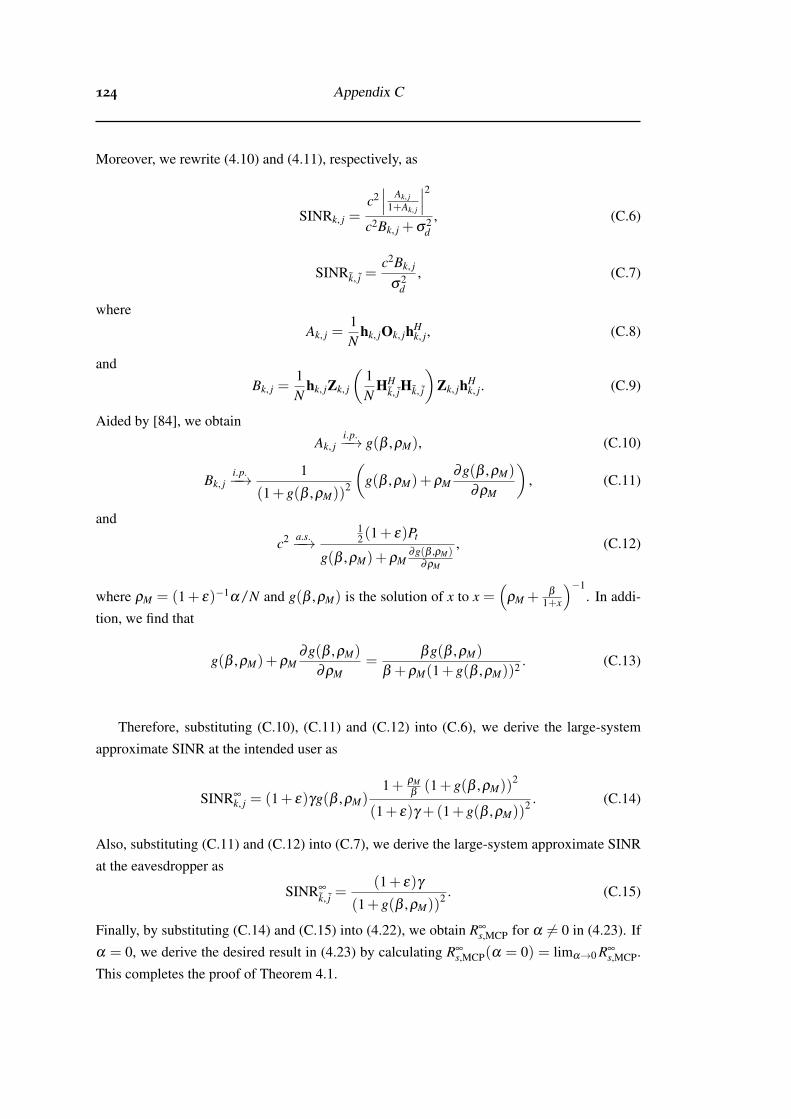
124 Appendix C
Moreover, we rewrite (4.10) and (4.11), respectively, as
SINRk, j =c2∣∣∣ Ak, j
1+Ak, j
∣∣∣2c2Bk, j +σ2
d, (C.6)
SINRk, j =c2Bk, j
σ2d
, (C.7)
where
Ak, j =1N
hk, jOk, jhHk, j, (C.8)
and
Bk, j =1N
hk, jZk, j
(1N
HHk, jHk, j
)Zk, jhH
k, j. (C.9)
Aided by [84], we obtain
Ak, ji.p.−−→ g(β ,ρM), (C.10)
Bk, ji.p.−−→ 1
(1+ g(β ,ρM))2
(g(β ,ρM)+ρM
∂g(β ,ρM)
∂ρM
), (C.11)
and
c2 a.s.−−→12 (1+ ε)Pt
g(β ,ρM)+ρM∂g(β ,ρM)
∂ρM
, (C.12)
where ρM = (1+ ε)−1α/N and g(β ,ρM) is the solution of x to x =(
ρM + β
1+x
)−1. In addi-
tion, we find that
g(β ,ρM)+ρM∂g(β ,ρM)
∂ρM=
βg(β ,ρM)
β +ρM(1+ g(β ,ρM))2 . (C.13)
Therefore, substituting (C.10), (C.11) and (C.12) into (C.6), we derive the large-system
approximate SINR at the intended user as
SINR∞k, j = (1+ ε)γg(β ,ρM)
1+ ρMβ(1+ g(β ,ρM))
2
(1+ ε)γ +(1+ g(β ,ρM))2 . (C.14)
Also, substituting (C.11) and (C.12) into (C.7), we derive the large-system approximate SINR
at the eavesdropper as
SINR∞
k, j =(1+ ε)γ
(1+ g(β ,ρM))2 . (C.15)
Finally, by substituting (C.14) and (C.15) into (4.22), we obtain R∞s,MCP for α 6= 0 in (4.23). If
α = 0, we derive the desired result in (4.23) by calculating R∞s,MCP(α = 0) = limα→0 R∞
s,MCP.
This completes the proof of Theorem 4.1.

§C.2 Proof of Theorem 4.2 125
C.2 Proof of Theorem 4.2
We first derive the large-system approximations of the SINRs for message sk, j at the intended
receiver and the eavesdropper, based on which we obtain the large-system secrecy sum rate
with the aid of (4.22).
Let us define
A j =
(ρC +
1N
2
∑m=1
K
∑l=1
hHl,m, jhl,m, j
)−1
(C.16)
and
Ak j =
(ρC +
1N ∑
(l,m) 6=(k, j)
hHl,m, jhl,m, j
)−1
, (C.17)
where ρC = α/N. Due to the consideration of P1 = P2 = P, we have c j = c j′ = c in (4.19)
and (4.20). Then, (4.19) and (4.20) can be, respectively, rewritten as
SINRk, j =c2∣∣∣ 1
N hk, j, jAk jhHk, j, j
∣∣∣2∑(k′, j′) 6=(k, j)
c2
N θk, j +σ2d
, (C.18)
and
SINRk, j =∑(k′, j′) 6=(k, j)
c2
N θk, j
σ2d
, (C.19)
where θk, j = hk, j, j′Ak′ j′hHk′, j′, j′hk′, j′, j′Ak′ j′hH
k, j, j′ , θk, j = hk′, j′, jAk jhHk, j, jhk, j, jAk jhH
k′, j′, j, and
c2 =P
∑Kk=1 ‖wk. j‖2
=P
∑Kk=1
1N2 hk, j, jA2
k jhHk, j, j
. (C.20)
According to [84], we have
maxj=1,2,k≤K
∣∣∣∣ 1N
hk, j, jAk jhHk, j, j−
1N
Tr(A j)
∣∣∣∣ a.s−→ 0, (C.21)
maxj=1,2,k≤K
∣∣∣∣ 1N2 hk, j, jA2
k jhHk, j, j−
1N
Tr(A2j)
∣∣∣∣ a.s−→ 0, (C.22)
maxj, j′=1,2, k,k′≤K, (k, j) 6=(k′, j′)
∣∣∣∣ 1N
θk, j−ϑ j′
∣∣∣∣ a.s−→ 0, (C.23)
maxj, j′=1,2, k,k′≤K, (k, j) 6=(k′, j′)
∣∣∣∣ 1N
θk, j−ϑ j
∣∣∣∣ a.s−→ 0, (C.24)
126 Appendix C
where ϑ j′ =ω j j′
Tr(A2j′ )
N(1+ω j j′
Tr(A j′ )N
)2 , ϑ j =ω j j′
Tr(A2j )
N(1+ω j j′
Tr(A j)N
)2 , and
ω j j′ =
{1 if j = j′,
ε if j 6= j′.(C.25)
In addition, we find thatTr(A j)
N=
Tr(A j′)
Na.s.−−→ Λ, (C.26)
Tr(A2j)
N=
Tr(A2j′)
Na.s.−−→− ∂ Λ
∂ρC, (C.27)
where Λ is the solution of x to
x =1
ρC + β
1+x +βε
1+εx
. (C.28)
Therefore, we obtain the following approximations as
∣∣hk, j, jwk, j∣∣2 a.s.−−→ Λ2, (C.29)
∑(k′, j′) 6=(k, j)
∣∣hk, j, j′wk′, j′∣∣2 a.s.−−→−
(βε
(1+ εΛ)2 +β
(1+Λ)2
)∂ Λ∂ρC
, (C.30)
∑(k′, j′) 6=(k, j)
∣∣hk′, j′, jwk, j∣∣2 a.s.−−→−
(βε
(1+ εΛ)2 +β
(1+Λ)2
)∂ Λ∂ρC
, (C.31)
and
c2 a.s.−−→− P
β∂ Λ∂ρC
, (C.32)
with
− ∂ Λ∂ρC
=Λ
ρC + βε
(1+εΛ)2 +β
(1+Λ)2
. (C.33)
Substituting (C.29), (C.30) and (C.32) into (C.18), we derive large-system approximate
SINR at the intended user as
SINR∞k, j =
Λβ
(ρC + βε
(1+εΛ)2 +β
(1+Λ)2
)1γ+ ε
(1+εΛ)2 +1
(1+Λ)2
. (C.34)
Also, substituting (C.31) and (C.32) into (C.19), we derive derive large-system approximate

§C.2 Proof of Theorem 4.2 127
SINR at the eavesdropper as
SINR∞
k, j = γ
(ε
(1+ εΛ)2 +1
(1+Λ)2
), (C.35)
Finally, by substituting (C.34) and (C.35) into (4.22), we obtain R∞s,CBf for α 6= 0 in (4.24). If
α = 0, we derive the desired result in (4.24) by calculating R∞s,CBf(α = 0) = limα→0 R∞
s,CBf.
This completes the proof of Theorem 4.2.

128 Appendix C

Appendix D
Appendix D
D.1 Proof of Proposition 5.2
To determine the maximum achievable secrecy throughput, we need first obtain the optimal
rate parameters that maximize the secrecy throughput. The problem is formulated by
maxRb,Rs
η = exp(−2Rb−1
γb
)Rs, (D.1)
s.t. Rb ≥ Rs > 0. (D.2)
Given given any Rs, we find that ∂η/∂Rb is always less than 0. Hence given any Rs, it is wise
to have the minimum Rb, i.e., Rb = Rs, for maximizing η . Then, the problem changes to
maxRs
η (Rb = Rs) = exp(−2Rs−1
γb
)Rs, (D.3)
s.t. Rs > 0. (D.4)
Taking the first order derivative of η (Rb = Rs) with respect to Rs, we have
∂η (Rb = Rs)
∂Rs= exp
(−2Rs−1
γb
)(1− 2RsRs ln2
γb
)(D.5)
By solving for Rs in ∂η(Rb=Rs)∂Rs
= 0, we obtain the optimal value of Rs that maximizes η , which
is given by
R�s =W0(γb)
ln2. (D.6)
Finally, substituting Rs = R�s into (D.3) completes the proof of Proposition 5.2.
D.2 Proof of Proposition 5.3
As analyzed in Appendix D.1, given any Rs, it is wise to have the minimum Rb, i.e., Rb = Rs,
for maximizing η . Hence, we can obtain the feasible range of Rs for satisfying the throughput
129
130 Appendix D
constraint by solving Rs to the equation η (Rb = Rs) = Γ. The feasible range is given by
Rs,min ≤ Rs ≤ Rs,max.
From pout = exp(−2Rb−θRs−1
γe
), we find that minimizing pout is equivalent to maximizing
O1 = Rb−θRs. (D.7)
To minimize O1 in (D.7), it is wise to have the maximum Rb while satisfying the throughput
constraint, for any given Rs. From η = exp(−2Rb−1
γb
)Rs ≥ Γ, we have
Rb ≤ log2
(1− γb ln
ΓRs
). (D.8)
Hence, we obtain R∗b1 as (5.31). Then, we can rewrite the optimization problem as
maxRs
log2
(1− γb ln
ΓRs
)−θRs, (D.9)
s.t. Rs,min ≤ Rs ≤ Rs,max. (D.10)
Finally, by solving for Rs in the equation ∂O∂Rs
= 0 and considering the feasible range of Rs, we
obtain R∗s1 as (5.32). This completes the proof of Proposition 5.3.
D.3 Proof of Proposition 5.4
The feasible range of Rs for satisfying the throughput constraint is given as Rs,min≤Rs≤Rs,max.
From ∆ = 1− 1Rs ln2 exp
(1γe
)(Ei(−2Rb
γe
)−Ei
(−2Rb−Rs
γe
)), we find that maximizing ∆ is
equivalent to minimizing
O2 =1Rs
(Ei(−2Rb
γe
)−Ei
(−2Rb−Rs
γe
)). (D.11)
Given any Rs, we have
∂O2
∂Rb=
ln(2)Rs
(exp(−2Rb
γe
)− exp
(−2Rb−Rs
γe
))< 0. (D.12)
Hence given any Rs, it is wise to have the maximum Rb while satisfying the throughput con-
straint to minimize O2 in (D.11). Hence, we obtain R∗b2 as (5.34). Then, we rewrite the opti-
mization problem as
minRs
1Rs
(Ei
(−
1− γb ln ΓRs
γe
)−Ei
(−
1− γb ln ΓRs
γe2Rs
)), (D.13)
s.t. Rs,min ≤ Rs ≤ Rs,max. (D.14)

§D.3 Proof of Proposition 5.4 131
We find that the closed-form solution of R∗s2 is mathematically intractable. We can obtain R∗s2
by numerically solving the problem above. This completes the proof of Proposition 5.4.

132 Appendix D
Bibliography
[1] Cisco, “Cisco visual networking index: global mobile data traffic forecast update, 2014–
2019,” Inc. White Paper, Feb. 2015. (cited on page 1)
[2] M. Monahan and D. V. Dyke, “Mobile online retail payments forecast 2015,” Javelin
Strategy and Research, Report, July 2015. (cited on page 1)
[3] B. Schneier, “Cryptographic design vulnerabilities,” IEEE Computer, vol. 31, no. 9, pp.
26–33, Sept. 1998. (cited on page 1)
[4] G. Kapoor and S. Piramithu, “Vulnerabilities in some recently proposed rfid ownership
transfer protocols,” IEEE Commun. Lett., vol. 14, no. 3, pp. 260–262, Mar. 2010. (cited
on page 1)
[5] A. Barenghi, L. Breveglieri, I. Koren, and D. Naccache, “Fault injection attacks on
cryptographic devices: Theory, practice, and countermeasures,” Proc. IEEE, vol. 100,
no. 11, pp. 3056–3076, Nov. 2012. (cited on page 1)
[6] Y. Liang, H. V. Poor, and S. Shamai, “Information theoretic security,” Found. Trends
Commun. Inf. Theory, vol. 5, no. 4-5, pp. 355–580, 2008. (cited on page 1)
[7] R. Liu and W. Trappe, Securing Wireless Communications at the Physical Layer.
Springer, Norwell, 2009. (cited on page 1)
[8] E. Jorswieck, A. Wolf, and S. Gerbracht, Secrecy on the Physical Layer in Wireless
Networks. Telecommunications, In-Tech Publishers, 2010. (cited on page 1)
[9] M. Bloch and J. Barros, Physical-Layer Security: From Information Theory to Security
Engineering. Cambridge University Press, 2011. (cited on pages 1 and 91)
[10] X. Zhou, L. Song, and Y. Zhang, Physical Layer Security in Wireless Communications.
CRC Press, 2013. (cited on page 1)
[11] M. Bloch, J. Barros, M. R. D. Rodrigues, and S. W. McLaughlin, “Wireless information-
theoretic security,” IEEE Trans. Inf. Theory, vol. 54, no. 6, pp. 2515–2534, June 2008.
(cited on page 2)
[12] C. E. Shannon, “Communication theory of secrecy systems,” Bell Syst. Tech. J., vol. 28,
pp. 656–715, Oct. 1949. (cited on page 2)
133
134 BIBLIOGRAPHY
[13] A. D. Wyner, “The wire-tap channel,” Bell Syst. Tech. J., vol. 54, no. 8, pp. 1355–1387,
Oct. 1975. (cited on pages 3, 4, 24, 89, 91, and 95)
[14] I. Csiszár, “Almost independence and secrecy capacity,” Prob. Inf. Trans., vol. 32, no. 1,
pp. 40–47, Jan. 1996. (cited on page 3)
[15] S. K. Leung-Yan-Cheong and M. E. Hellman, “The Gaussian wire-tap channel,” IEEE
Trans. Inf. Theory, vol. 24, no. 4, pp. 451–456, July 1978. (cited on pages 4, 51, 91, 92,
and 96)
[16] P. K. Gopala, L. Lai, and H. El Gamal, “On the secrecy capacity of fading channels,”
IEEE Trans. Inf. Theory, vol. 54, no. 10, pp. 4687–4698, Oct. 2008. (cited on pages 4,
5, 6, 13, and 20)
[17] P. Parada and R. Blahut, “Secrecy capacity of SIMO and slow fading channels,” in Proc.
IEEE ISIT, Adelaide, SA, Sept. 2005, pp. 2152–2155. (cited on page 5)
[18] J. Barros and M. R. D. Rodrigues, “Secrecy capacity of wireless channels,” in Proc.
IEEE ISIT, Seattle, WA, July 2006, pp. 356–360. (cited on page 5)
[19] X. Zhou, M. R. McKay, B. Maham, and A. Hjørungnes, “Rethinking the secrecy outage
formulation: A secure transmission design perspective,” IEEE Commun. Lett., vol. 15,
no. 3, pp. 302–304, Mar. 2011. (cited on pages 5, 6, 13, 25, 95, and 96)
[20] Z. Rezki, A. Khisti, and M.-S. Alouini, “On the ergodic secrecy capacity of the wiretap
channel under imperfect main channel estimation,” in Proc. Asilomar Conf. Signals Syst.
Comput., Pacific Grove, CA, Nov. 2011, pp. 952–957. (cited on page 6)
[21] T.-X. Zheng, H.-M. Wang, and Q. Yin, “On transmission secrecy outage of a multi-
antenna system with randomly located eavesdroppers,” IEEE Commun. Lett., vol. 18,
no. 8, pp. 1299–1302, Aug. 2014. (cited on page 6)
[22] C. Wang and H.-M. Wang, “On the secrecy throughput maximization for MISO cogni-
tive radio network in slow fading channels,” IEEE Trans. Inf. Forensics Security, vol. 9,
no. 11, pp. 1814–1827, Nov. 2014. (cited on page 6)
[23] S. Yan, G. Geraci, N. Yang, R. Malaney, and J. Yuan, “On the target secrecy rate for
SISOME wiretap channels,” in Proc. IEEE ICC, June 2014, pp. 987–992. (cited on
page 6)
[24] A. O. Hero, “Secure space-time communication,” IEEE Trans. Inf. Theory, vol. 49,
no. 12, pp. 3235–3249, Dec. 2003. (cited on page 7)
BIBLIOGRAPHY 135
[25] A. Mukherjee, S. A. A. Fakoorian, J. Huang, and A. L. Swindlehurst, “Principles of
physical layer security in multiuser wireless networks: A survey,” IEEE Commun. Sur-
veys Tutorials, vol. 16, no. 3, pp. 1550–1573, Third 2014. (cited on page 7)
[26] R. Negi and S. Goel, “Secret communication using artificial noise,” in Proc. IEEE VTC,
vol. 3, Dallas, TX, Sept. 2005, pp. 1906–1910. (cited on page 7)
[27] S. Goel and R. Negi, “Guaranteeing secrecy using artificial noise,” IEEE Trans. Wireless
Commun., vol. 7, no. 6, pp. 2180–2189, June 2008. (cited on pages 7, 11, 45, and 50)
[28] X. Zhou and M. R. McKay, “Secure transmission with artificial noise over fading chan-
nels: Achievable rate and optimal power allocation,” IEEE Trans. Veh. Technol., vol. 59,
no. 8, pp. 3831–3842, Oct. 2010. (cited on pages 8, 11, 19, 20, and 45)
[29] N. Romero-Zurita, M. Ghogho, and D. McLernon, “Outage probability based power
distribution between data and artificial noise for physical layer security,” IEEE Signal
Process. Lett., vol. 19, no. 2, pp. 71–74, Feb. 2012. (cited on page 8)
[30] N. Romero-Zurita, D. McLernon, M. Ghogho, and A. Swami, “PHY layer security
based on protected zone and artificial noise„” IEEE Signal Process. Lett., vol. 20, no. 5,
pp. 487–490, May 2013. (cited on page 8)
[31] J. Huang and A. L. Swindlehurst, “Robust secure transmission in MISO channels based
on worst-case optimization,” IEEE Trans. Signal Process., vol. 60, no. 4, pp. 1696–1707,
Apr. 2012. (cited on pages 8, 10, and 19)
[32] S. Gerbracht, C. Scheunert, and E. A. Jorswieck, “Secrecy outage in MISO systems
with partial channel information,” IEEE Trans. Inf. Forensics Security, vol. 7, no. 2, pp.
704–716, Apr. 2012. (cited on page 8)
[33] A. L. Swindlehurst, “Fixed SINR solutions for the MIMO wiretap channel,” in Proc.
IEEE ICASSP, Taipei, Taiwan, Apr. 2009, pp. 2437–2440. (cited on page 8)
[34] A. Mukherjee and A. L. Swindlehurst, “Fixed-rate power allocation strategies for en-
hanced secrecy in MIMO wiretap channels,” in Proc. IEEE SPAWC Workshop, Perugia,
Italy, June 2009, pp. 344–348. (cited on page 8)
[35] ——, “Utility of beamforming strategies for secrecy in multiuser MIMO wiretap chan-
nels,” in Proc. Allerton Conf. Commun., Control Computing, Monticello, IL, Oct. 2009,
pp. 1134–1140. (cited on page 8)
[36] J. M. Taylor, M. Hempel, H. Sharif, S. Ma, and Y. Yang, “Impact of channel estima-
tion errors on effectiveness of eigenvector-based jamming for physical layer security in
136 BIBLIOGRAPHY
wireless networks,” in Proc. IEEE CAMAD Workshop, Kyoto, Japan, June 2011, pp.
122–126. (cited on pages 8, 19, and 20)
[37] A. Mukherjee and A. L. Swindlehurst, “Robust beamforming for security in MIMO
wiretap channels with imperfect CSI,” IEEE Trans. Signal Process., vol. 59, no. 1, pp.
351–361, Jan. 2011. (cited on pages 8, 10, 11, 19, and 45)
[38] T.-Y. Liu, S.-C. Lin, T.-H. Chang, and Y.-W. P. Hong, “How much training is enough
for secrecy beamforming with artificial noise,” in Proc. IEEE ICC, Ottawa, ON, June
2012, pp. 4782–4787. (cited on pages 8, 19, and 20)
[39] R. Liu, T. Liu, H. V. Poor, and S. Shamai, “Multiple-input multiple-output Gaussian
broadcast channels with confidential messages,” IEEE Trans. Inf. Theory, vol. 56, no. 9,
pp. 4215–4227, Sept. 2010. (cited on page 9)
[40] D. A. A. Fakoorian and A. L. Swindlehurst, “MIMO interference channel with con-
fidential messages: Achievable secrecy rates and precoder design,” IEEE Trans. Inf.
Forensics Security, vol. 6, no. 3, pp. 640–649, Sept. 2011. (cited on page 9)
[41] G. Geraci, M. Egan, J. Yuan, A. Razi, and I. B. Collings, “Secrecy sum-rates for multi-
user MIMO regularized channel inversion precoding,” IEEE Trans. Commun., vol. 60,
no. 11, pp. 3472–3482, Nov. 2012. (cited on pages 9, 67, and 70)
[42] G. Geraci, J. Yuan, and I. B. Collings, “Large system analysis of the secrecy sum-rates
with regularized channel inversion precoding,” in Proc. IEEE WCNC, Apr. 2012, pp.
533–537. (cited on page 9)
[43] G. Geraci, R. Couillet, J. Yuan, M. Debbah, and I. B. Collings, “Large system analysis
of linear precoding in MISO broadcast channels with confidential messages,” IEEE J.
Sel. Areas Commun., vol. 31, no. 9, pp. 1660–1671, Sept. 2013. (cited on pages 9, 67,
70, 71, 76, and 84)
[44] G. Geraci, A. Y. Al-Nahari, J. Yuan, and I. B. Collings, “Linear precoding for broad-
cast channels with confidential messages under transmit-side channel correlation,” IEEE
Commun. Lett., vol. 17, no. 6, pp. 1164–1167, June 2013. (cited on pages 9, 67, and 70)
[45] N. Yang, G. Geraci, J. Yuan, and R. Malaney, “Confidential broadcasting via linear
precoding in non-homogeneous MIMO multiuser networks,” IEEE Trans. Commun.,
vol. 62, no. 7, pp. 2515–2530, July 2014. (cited on pages 9, 67, 70, and 71)
[46] D. W. K. Ng, E. S. Lo, and R. Schober, “Resource allocation for secure OFDMA net-
works with imperfect CSIT,” in Proc. IEEE GLOBECOM, Houston, TX, Dec. 2011, pp.
1–6. (cited on pages 10 and 19)
BIBLIOGRAPHY 137
[47] Q. Li and W.-K. Ma, “Optimal and robust transmit designs for MISO channel secrecy by
semidefinite programming,” IEEE Trans. Signal Process., vol. 59, no. 8, pp. 3799–3812,
Aug. 2011. (cited on pages 10 and 19)
[48] S.-C. Lin, T.-H. Chang, Y.-L. Liang, Y.-W. P. Hong, and C.-Y. Chi, “On the impact
of quantized channel feedback in guaranteeing secrecy with artificial noise: The noise
leakage problem,” IEEE Trans. Wireless Commun., vol. 10, no. 3, pp. 901–915, Mar.
2011. (cited on pages 10 and 19)
[49] A. Khisti and G. W. Wornell, “Secure transmission with multiple antennas I: The MI-
SOME wiretap channel,” IEEE Trans. Inf. Theory, vol. 56, no. 7, pp. 3088–3104, July
2010. (cited on pages 11 and 45)
[50] ——, “Secure transmission with multiple antennas–Part II: The MIMOME wiretap
channel,” IEEE Trans. Inf. Theory, vol. 56, no. 11, pp. 5515–5532, Nov. 2010. (cited
on pages 11 and 45)
[51] F. Oggier and B. Hassibi, “The secrecy capacity of the MIMO wiretap channel,” IEEE
Trans. Inf. Theory, vol. 57, no. 8, pp. 4961–4972, Aug. 2011. (cited on pages 11 and 45)
[52] X. Zhou, R. K. Ganti, and J. G. Andrews, “Secure wireless network connectivity with
multi-antenna transmission,” IEEE Trans. Wireless Commun., vol. 10, no. 2, pp. 425–
430, Feb. 2011. (cited on pages 11 and 45)
[53] N. Yang, P. L. Yeoh, M. Elkashlan, R. Schober, and I. B. Collings, “Transmit antenna
selection for security enhancement in MIMO wiretap channels,” IEEE Trans. Commun.,
vol. 61, no. 1, pp. 144–154, Jan. 2013. (cited on pages 11 and 45)
[54] D. Klinc, J. Ha, S. W. McLaughlin, J. Barros, and B. J. Kwak, “LDPC codes for the
Gaussian wiretap channel,” IEEE Trans. Inf. Forensics Security, vol. 6, no. 3, pp. 532–
540, Sept. 2011. (cited on page 12)
[55] M. Baldi, M. Bianchi, and F. Chiaraluce, “Coding with scrambling, concatenation, and
HARQ for the AWGN wire-tap channel: A security gap analysis,” IEEE Trans. Inf.
Forensics Security, vol. 7, no. 3, pp. 883–894, June 2012. (cited on page 12)
[56] K. Guan, P. J. Winzer, A. M. Tulino, and E. Soljanin, “An error probability approach for
quantifying physical layer security of MIMO-SDM systems,” in Proc. Eur. Conf. Opt.
Commun., Sept. 2014, pp. 1–3. (cited on page 12)
[57] M. Baldi, G. Ricciutelli, N. Maturo, and F. Chiaraluce, “Performance assessment and
design of finite length LDPC codes for the Gaussian wiretap channel,” in Proc. IEEE
ICC Workshops, June 2015, pp. 446–451. (cited on page 12)

138 BIBLIOGRAPHY
[58] D. Gesbert, S. Hanly, H. Huang, S. S. Shitz, O. Simeone, and W. Yu, “Multi-cell MIMO
cooperative networks: A new look at interference,” IEEE J. Sel. Areas Commun., vol. 28,
no. 9, pp. 1380–1408, Dec. 2010. (cited on page 15)
[59] C. B. Peel, B. M. Hochwald, and A. L. Swindlehurst, “A vector-perturbation technique
for near-capacity multiantenna multiuser communication–Part I: Channel inversion and
regularization,” IEEE Trans. Commun., vol. 53, no. 1, pp. 195–202, Jan. 2005. (cited
on pages 15 and 71)
[60] R. Zakhour and S. Hanly, “Base station cooperation on the downlink: Large system
analysis,” IEEE Trans. Inf. Theory, vol. 58, no. 4, pp. 2079–2106, Apr. 2012. (cited on
pages 15, 69, and 73)
[61] X. Zhou, P. Sadeghi, T. A. Lamahewa, and S. Durrani, “Design guidelines for training-
based MIMO systems with feedback,” IEEE Trans. Signal Process., vol. 57, no. 10, pp.
4014–4026, Oct. 2009. (cited on page 19)
[62] L. H. Ozarow, S. Shamai, and A. D. Wyner, “Information theoretic considerations for
cellular mobile radio,” IEEE Trans. Veh. Technol, vol. 43, no. 2, pp. 359–378, May 1994.
(cited on page 20)
[63] S. M. Kay, Fundamentals of Statistical Signal Processing: Estimation Theory. Engle-
wood Cliffs, NJ: PTR Prentice Hall, 1993. (cited on page 22)
[64] J. K. Cavers, “An analysis of pilot symbol assisted modulation for Rayleigh fading chan-
nels,” IEEE Trans. Veh. Technol., vol. 40, no. 4, pp. 686–693, Nov. 1991. (cited on page
22)
[65] B. Hassibi and B. M. Hochwald, “How much training is needed in multiple-antenna
wireless links?” IEEE Trans. Inf. Theory, vol. 49, no. 4, pp. 951–963, Apr. 2003. (cited
on page 22)
[66] A. Vakili, M. Sharif, and B. Hassibi, “The effect of channel estimation error on the
throughput of broadcast channels,” in Proc. IEEE ICASSP, vol. 4, Toulouse, France,
May 2006. (cited on page 22)
[67] A. Thangaraj, S. Dihidar, A. R. Calderbank, S. W. McLaughlin, and J.-M. Merolla,
“Applications of LDPC codes to the wiretap channel,” IEEE Trans. Inf. Theory, vol. 53,
no. 8, pp. 2933–2945, Aug. 2007. (cited on page 24)
[68] X. Tang, R. Liu, Sapsojevic, and H. V. Poor, “On the throughput of secure hybrid-ARQ
protocols for Gaussian block-fading channels,” IEEE Trans. Inf. Theory, vol. 55, no. 4,
pp. 1575–1590, Apr. 2009. (cited on page 24)
BIBLIOGRAPHY 139
[69] J. I. Marcum, Table of Q Functions. U.S. Air Force Project RAND Research Memo-
randum M-339, ASTIA Document AD 1165451, Rand Corporation, Santa Monica, CA,
1950. (cited on page 29)
[70] T. S. Pollock, “On limits of multi-antenna wireless communications in spatially
selective channels,” Ph.D. dissertation, The Australian National University, Australia,
July 2003. [Online]. Available: http://hdl.handle.net/1885/47999 (cited on pages 46,
52, and 117)
[71] E. G. Larsson, O. Edfors, F. Tufvesson, and T. Marzetta, “Massive MIMO for next
generation wireless systems,” IEEE Commun. Mag., vol. 52, no. 2, pp. 186–195, Feb.
2014. (cited on page 46)
[72] J. G. Andrews, S. Buzzi, W. Choi, S. V. Hanly, A. Lozano, A. C. K. Soong, and J. C.
Zhang, “What will 5G be?” IEEE J. Sel. Areas Commun., vol. 32, no. 6, pp. 1065–1082,
June 2014. (cited on page 46)
[73] T. S. Pollock, T. D. Abhayapala, and R. A. Kennedy, “Introducing space into MIMO
capacity calculations,” J. Telecommun. Syst., vol. 24, no. 2, pp. 415–436, Oct. 2003.
(cited on page 46)
[74] T. D. Abhayapala, R. A. Kennedy, and J. T. Y. Ho, “On capacity of multi-antenna wire-
less channels: Effects of antenna separation and spatial correlation,” in Proc. IEEE
AusCTW, Canberra, Australia, Feb. 2002, pp. 4–5. (cited on page 46)
[75] T. S. Pollock, T. D. Abhayapala, and R. A. Kennedy, “Introducing ‘space’ into space-
time MIMO capacity calculations: A new closed form upper bound,” in Proc. ICT,
vol. 2, Feb. 2003, pp. 1536–1541. (cited on page 46)
[76] R. A. Kennedy, P. Sadeghi, T. D. Abhayapala, and H. M. Jones, “Intrinsic limits of
dimensionality and richness in random multipath fields,” IEEE Trans. Signal Process.,
vol. 55, no. 6, pp. 2542–2556, June 2007. (cited on page 46)
[77] F. Bashar and T. D. Abhayapala, “Degrees of freedom of band limited signals measured
over space,” in Proc. ISCIT, Oct. 2012, pp. 735–740. (cited on page 46)
[78] F. Bashar, S. M. A. Salehin, and T. D. Abhayapala, “Analysis of degrees of freedom
of wideband random multipath fields observed over time and space windows,” in Proc.
IEEE Workshop SSP, June 2014, pp. 45–48. (cited on page 46)
[79] ——, “Band limited signals observed over finite spatial and temporal windows: An
upper bound to signal degrees of freedom,” submitted to IEEE Trans. Signal Process.,
2014. [Online]. Available: http://arxiv.org/abs/1405.2163 (cited on page 46)
140 BIBLIOGRAPHY
[80] D. Gesbert, T. Ekman, and N. Christophersen, “Capacity limits of dense palm-sized
MIMO arrays,” in Proc. IEEE GLOBECOM, vol. 2, Nov. 2002, pp. 1187–1191. (cited
on page 52)
[81] L. Hanlen and M. Fu, “Capacity of MIMO wireless systems with spatially correlated
receive elements,” in Proc. WITSP, Wollongong, Australia, Dec. 2002, pp. 1–6. (cited
on page 52)
[82] T. S. Pollock, T. D. Abhayapala, and R. A. Kennedy, “Antenna saturation effects on
MIMO capacity,” in Proc. IEEE ICC, vol. 4, May 2003, pp. 2301–2305. (cited on page
52)
[83] Y. Wu and Z. Nie, “On the MIMO channel capacity saturation for spatially constrained
receive region,” J. Systems Engineering Electronics, vol. 18, no. 3, pp. 437–442, Sept.
2007. (cited on page 52)
[84] R. Muharar, R. Zakhour, and J. Evans, “Base station cooperation with feedback opti-
mization: A large system analysis,” IEEE Trans. Inf. Theory, vol. 60, no. 6, pp. 3620–
3644, June 2014. (cited on pages 69, 79, 80, 124, and 125)
[85] H. Dahrouj and W. Yu, “Coordinated beamforming for the multicell multi-antenna wire-
less system,” IEEE Trans. Wireless Commun., vol. 9, no. 5, pp. 1748–1759, May 2010.
(cited on page 73)
[86] Q. H. Spencer, A. L. Swindlehurst, and M. Haardt, “Zero-forcing methods for down-
link spatial multiplexing in multiuser MIMO channels,” IEEE Trans. Signal Process.,
vol. 52, no. 2, pp. 461–471, Feb. 2004. (cited on page 83)
[87] H. Sung, S.-R. Lee, and I. Lee, “Generalized channel inversion methods for multiuser
MIMO systems,” IEEE Trans. Commun., vol. 57, no. 11, pp. 3489–3499, Nov. 2009.
(cited on page 83)
[88] Z. Shen, R. Chen, J. G. Andrews, R. W. Heath, and B. L. Evans, “Low complexity user
selection algorithms for multiuser MIMO systems with block diagonalization,” IEEE
Trans. Signal Process., vol. 54, no. 9, pp. 3658–3663, Sept. 2006. (cited on page 83)
[89] I. Csiszár and J. Körner, “Broadcast channels with confidential messages,” IEEE Trans.
Inf. Theory, vol. 24, no. 3, pp. 339–348, May 1978. (cited on page 89)
[90] T. M. Cover and J. A. Thomas, Elements of Information Theory, 2nd ed. Wiley, 2006.
(cited on pages 89 and 91)
[91] M. Feder and N. Merhav, “Relations between entropy and error probability,” IEEE
Trans. Inf. Theory, vol. 40, no. 1, pp. 259–266, Jan. 1994. (cited on pages 89 and 91)
BIBLIOGRAPHY 141
[92] Y. Liang, H. V. Poor, and S. Shamai, “Secure communication over fading channels,”
IEEE Trans. Inf. Theory, vol. 54, no. 6, pp. 2470–2492, June 2008. (cited on pages 92
and 96)
[93] B. He and X. Zhou, “Secure on-off transmission design with channel estimation errors,”
IEEE Trans. Inf. Forensics Security, vol. 8, no. 12, pp. 1923–1936, Dec. 2013. (cited
on page 95)
[94] J. Kiefer, “Sequential minimax search for a maximum,” Proc. Amer. Math. Soc., vol. 4,
no. 3, pp. 502–506, 1953. (cited on page 103)
[95] X. Zhou, P. Sadeghi, T. A. Lamahewa, and S. Durrani, “Optimizing antenna config-
uration for MIMO systems with imperfect channel estimation,” IEEE Trans. Wireless
Commun., vol. 8, no. 3, pp. 1177–1181, Mar. 2009. (cited on page 110)
[96] M. Haenggi, J. Andrews, F. Baccelli, O. Dousse, and M. Franceschetti, “Stochastic
geometry and random graphs for the analysis and design of wireless networks,” IEEE J.
Sel. Areas Commun., vol. 27, no. 7, pp. 1029–1046, Sept. 2012. (cited on page 110)
[97] F. Baccelli, B. Blaszczyszyn, and P. Miihlethaler, “Stochastic analysis of spatial and
opportunistic ALOHA,” IEEE J. Select. Areas Commun., vol. 27, no. 7, pp. 1105–1119,
Sept. 2009. (cited on page 110)
[98] S. Weber and J. G. Andrews, Transmission Capacity of Wireless Networks, 1st ed. Now
Publishers Inc., 2012. (cited on page 110)
[99] S. Srinivasa and M. Haenggi, “Distance distributions in finite uniformly random net-
works: Theory and applications,” IEEE Trans. Veh. Technol., vol. 59, no. 2, pp. 940–949,
Feb. 2010. (cited on page 110)
[100] Z. Khalid and S. Durrani, “Distance distributions in regular polygons,” IEEE Trans. Veh.
Technol., vol. 62, no. 5, pp. 2363–2368, June 2013. (cited on page 110)
[101] P. C. Pinto, J. Barros, and M. Z. Win, “Secure communication in stochastic wireless
networks – Part I: Connectivity,” IEEE Trans. Inf. Forensics Security, vol. 7, no. 1, pp.
125–138, Feb. 2012. (cited on page 110)
[102] O. O. Koyluoglu, C. E. Koksal, and H. E. Gamal, “On secrecy capacity scaling in wire-
less networks,” IEEE Trans. Inform. Theory, vol. 58, no. 5, pp. 3000–3015, May. 2012.
(cited on page 110)
[103] H. Wang, X. Zhou, and M. C. Reed, “Physical layer security in cellular networks:
A stochastic geometry approach,” IEEE Trans. Wireless Commun., vol. 12, no. 6, pp.
2776–2787, June 2013. (cited on page 110)

142 BIBLIOGRAPHY
[104] A. Bayesteh, M. Ansari, and A. K. Khandani, “Effect of jamming on the capacity of
MIMO channels,” in Proc. Allerton, Oct. 2004, pp. 401–410. (cited on page 117)