Embed Size (px)
Citation preview

Wireless Sensor Networks: Development of an Environmental Data Acquisition Prototype System and Graphical
User Interface.
A Thesis Presented to the Faculty of
California Polytechnic State University San Luis Obispo
In Partial Fulfillment of the Requirements for the Degree
Master of Science in Electrical Engineering
by Jose A Becerra-Maciel
November 2006
ii
Authorization for Reproduction of Master’s Thesis I grant permission for the reproduction of this thesis in its entirety or any of its parts, without further authorization from me. _____________________________ Signature (Jose A Becerra-Maciel) _____________________________ Date
iii
Approval Page
Title: Development of an Environmental Data Acquisition Prototype
System and Graphical User Interface. Author : Jose A Becerra-Maciel Date Submitted: November 17, 2006 Dr. James Harris _____________________________
Advisor and Committee Chair Signature Dr. Fred W. DePiero ____________________________ Committee Member Signature Dr. Diana Franklin ____________________________ Committee Member Signature

iv
Abstract
Wireless Sensor Networks: Development of an Environmental Data Acquisition Prototype System and Graphical User Interface.
Jose A. Becerra-Maciel Wireless Sensor Networks (WSN), small radio transmitting sensors called “motes” promise to change how scientists gather environmental data in various disciplines. For example, a group of biologists studying the perfect ambient conditions for the survival of the endangered species of redwood tree in Sonoma California in the past had to climb with three hardwired 30-pound sensors up to 30 meters height to gather temperature and humidity readings. With WSN technology, the biologists deploy up to 50 tiny wireless computers in the same tree at different heights gathering much more information and with less effort [39]. David Culler, leading computer scientist of WSN at Intel Labs in Berkeley, California explains that 50 to 100 motes are being deployed at the Golden Gate Bridge in San Francisco to study the effects on vibrations from traffic, wind and earthquakes on the bridge. Motes are useful for more than research; according to David “these motes are going to change our lives” [39]. He adds: “ There are so many of the things we do in society that could be much efficient if we have the same ability to see what’s going on across a broad area of space with many objects in it”[39]. This project applies the state of the art technology of WSN to gather and display environmental sensor readings such as: temperature, pressure, relative humidity, wind speed/direction, rain fall level and GPS, from the environment. It explains the process of adding sensors to the system and combines research done by Cal Poly undergraduate students to accomplish the objective.

v
Acknowledgements
I would like to thank my family, who gave me the strength to continue my education; without them this research would not be possible. Thanks to Dr. Harris for giving me the opportunity to work on the Wireless Sensor Network Group and for his patience and motivation to finish this thesis work. Thanks Dr. John Seng and Dr. Diana Franklin for sharing the Crossbow hardware acquired from their Cal Poly Central Coast Research Park (C3RP) award, which was necessitated by this thesis.
vi
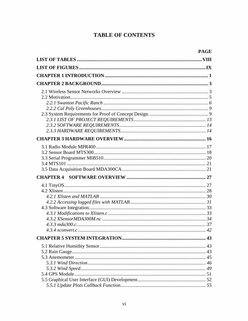
TABLE OF CONTENTS
PAGE
LIST OF TABLES .......................................................................................................VIII
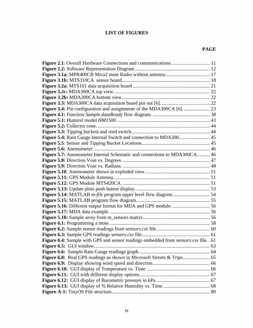
LIST OF FIGURES ........................................................................................................ IX
CHAPTER 1 INTRODUCTION..................................................................................... 1
CHAPTER 2 BACKGROUND........................................................................................ 3 2.1 Wireless Sensor Networks Overview ....................................................................... 3 2.2 Motivation................................................................................................................. 5
2.2.1 Swanton Pacific Ranch ...................................................................................... 6 2.2.2 Cal Poly Greenhouses........................................................................................ 9
2.3 System Requirements for Proof of Concept Design. ................................................ 9 2.3.1 LIST OF PROJECT REQUIREMENTS........................................................... 13 2.3.2 SOFTWARE REQUIREMENTS....................................................................... 14 2.3.3 HARDWARE REQUIREMENTS...................................................................... 14
CHAPTER 3 HARDWARE OVERVIEW ................................................................... 16 3.1 Radio Module MPR400 .......................................................................................... 17 3.2 Sensor Board MTS300............................................................................................ 18 3.3 Serial Programmer MIB510.................................................................................... 20 3.4 MTS101 .................................................................................................................. 21 3.5 Data Acquisition Board MDA300CA..................................................................... 21
CHAPTER 4 SOFTWARE OVERVIEW ................................................................. 27 4.1 TinyOS.................................................................................................................... 27 4.2 Xlisten ..................................................................................................................... 28
4.2.1 Xlisten and MATLAB ....................................................................................... 30 4.2.2 Accessing logged files with MATLAB.............................................................. 31
4.3 Software Integration................................................................................................ 33 4.3.1 Modifications to Xlisten.c ................................................................................ 33 4.3.2 XSensorMDA300M.nc ..................................................................................... 34 4.3.3 mda300.c.......................................................................................................... 37 4.3.4 xconvert.c ......................................................................................................... 42
CHAPTER 5 SYSTEM INTEGRATION..................................................................... 43 5.1 Relative Humidity Sensor ....................................................................................... 43 5.2 Rain Gauge.............................................................................................................. 43 5.3 Anemometer............................................................................................................ 45
5.3.1 Wind Direction................................................................................................. 46 5.3.2 Wind Speed....................................................................................................... 49
5.4 GPS Module............................................................................................................ 51 5.5 Graphical User Interface (GUI) Development........................................................ 52
5.5.1 Update Plots Callback Function...................................................................... 55
vii
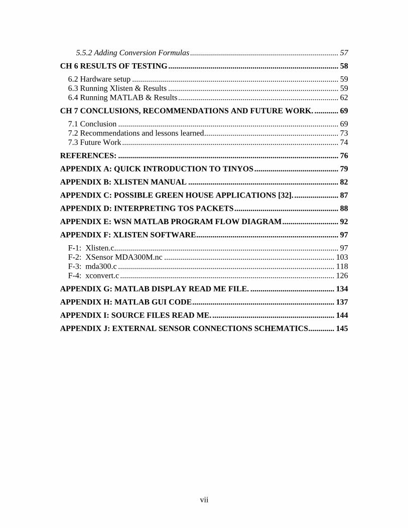
5.5.2 Adding Conversion Formulas .......................................................................... 57
CH 6 RESULTS OF TESTING..................................................................................... 58 6.2 Hardware setup ....................................................................................................... 59 6.3 Running Xlisten & Results ..................................................................................... 59 6.4 Running MATLAB & Results ................................................................................ 62
CH 7 CONCLUSIONS, RECOMMENDATIONS AND FUTURE WORK. ............ 69 7.1 Conclusion .............................................................................................................. 69 7.2 Recommendations and lessons learned................................................................... 73 7.3 Future Work ............................................................................................................ 74
REFERENCES: .............................................................................................................. 76
APPENDIX A: QUICK INTRODUCTION TO TINYOS.......................................... 79
APPENDIX B: XLISTEN MANUAL ........................................................................... 82
APPENDIX C: POSSIBLE GREEN HOUSE APPLICATIONS [32]. ...................... 87
APPENDIX D: INTERPRETING TOS PACKETS.................................................... 88
APPENDIX E: WSN MATLAB PROGRAM FLOW DIAGRAM............................ 92
APPENDIX F: XLISTEN SOFTWARE....................................................................... 97 F-1: Xlisten.c................................................................................................................ 97 F-2: XSensor MDA300M.nc ..................................................................................... 103 F-3: mda300.c ............................................................................................................ 118 F-4: xconvert.c ........................................................................................................... 126
APPENDIX G: MATLAB DISPLAY READ ME FILE. .......................................... 134
APPENDIX H: MATLAB GUI CODE....................................................................... 137
APPENDIX I: SOURCE FILES READ ME. ............................................................. 144
APPENDIX J: EXTERNAL SENSOR CONNECTIONS SCHEMATICS............. 145
viii
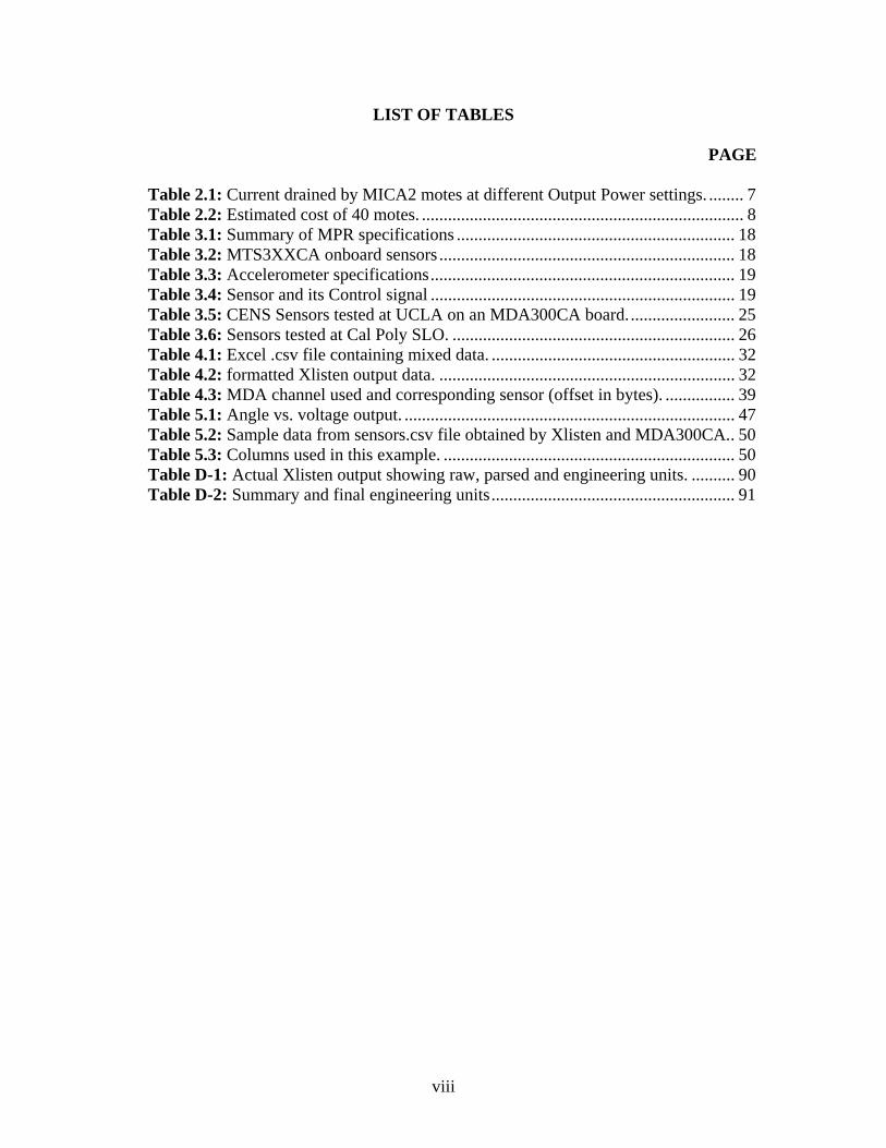
LIST OF TABLES
PAGE
Table 2.1: Current drained by MICA2 motes at different Output Power settings. ........ 7 Table 2.2: Estimated cost of 40 motes. .......................................................................... 8 Table 3.1: Summary of MPR specifications ................................................................ 18 Table 3.2: MTS3XXCA onboard sensors .................................................................... 18 Table 3.3: Accelerometer specifications...................................................................... 19 Table 3.4: Sensor and its Control signal ...................................................................... 19 Table 3.5: CENS Sensors tested at UCLA on an MDA300CA board......................... 25 Table 3.6: Sensors tested at Cal Poly SLO. ................................................................. 26 Table 4.1: Excel .csv file containing mixed data. ........................................................ 32 Table 4.2: formatted Xlisten output data. .................................................................... 32 Table 4.3: MDA channel used and corresponding sensor (offset in bytes). ................ 39 Table 5.1: Angle vs. voltage output. ............................................................................ 47 Table 5.2: Sample data from sensors.csv file obtained by Xlisten and MDA300CA.. 50 Table 5.3: Columns used in this example. ................................................................... 50 Table D-1: Actual Xlisten output showing raw, parsed and engineering units. .......... 90 Table D-2: Summary and final engineering units........................................................ 91
ix
LIST OF FIGURES
PAGE
Figure 2.1: Overall Hardware Connections and communications ............................... 11 Figure 2.2: Software Representation Diagram ............................................................ 12 Figure 3.1a: MPR400CB Mica2 mote Radio without antenna.................................... 17 Figure 3.1b: MTS310CA sensor board....................................................................... 18 Figure 3.2a: MTS101 data acquisition board .............................................................. 21 Figure 3.2c: MDA300CA top view. ............................................................................ 22 Figure 3.2b: MDA300CA bottom view....................................................................... 22 Figure 3.3: MDA300CA data acquisition board pin out [6]........................................ 22 Figure 3.4: Pin configuration and assignments of the MDA300CA [6]. ..................... 23 Figure 4.1: Function Sample.dataReady flow diagram. .............................................. 38 Figure 5.1: Humirel model HM1500. .......................................................................... 43 Figure 5.2: Collector cone. .......................................................................................... 44 Figure 5.3: Tipping buckets and reed switch............................................................... 44 Figure 5.4: Rain Gauge Internal Switch and connection to MDA300......................... 45 Figure 5.5: Sensor and Tipping Bucket Locations....................................................... 45 Figure 5.6: Anemometer. ............................................................................................. 46 Figure 5.7: Anemometer Internal Schematic and connections to MDA300CA. ......... 46 Figure 5.8: Direction Vout vs. Degrees. ...................................................................... 47 Figure 5.9: Direction Vout vs. Radians. ...................................................................... 48 Figure 5.10: Anemometer shown in exploded view. ................................................... 51 Figure 5.11: GPS Module Antenna.............................................................................. 51 Figure 5.12: GPS Module MTS420CA. ...................................................................... 51 Figure 5.13: Update plots push button display. ........................................................... 53 Figure 5.14: MATLAB m-file program upper level flow diagram.............................. 54 Figure 5.15: MATLAB program flow diagram. .......................................................... 55 Figure 5.16: Different output format for MDA and GPS module. .............................. 56 Figure 5.17: MDA data example. ................................................................................ 56 Figure 5.18: Sample array from m_sensors matrix...................................................... 56 Figure 6.1: Programming a mote. ................................................................................ 58 Figure 6.2: Sample sensor readings from sensors.csv file. .......................................... 60 Figure 6.3: Sample GPS readings sensors.csv file....................................................... 61 Figure 6.4: Sample with GPS and sensor readings embedded from sensors.csv file. . 61 Figure 6.5: GUI window............................................................................................. 63 Figure 6.6: Sample Rain Gauge readings graph. ........................................................ 64 Figure 6.8: Real GPS readings as shown in Microsoft Streets & Trips...................... 65 Figure 6.9: Display showing wind speed and direction.............................................. 66 Figure 6.10: GUI display of Temperature vs. Time ................................................... 66 Figure 6.11: GUI with different display options......................................................... 67 Figure 6.12: GUI display of Barometric pressure in kPa. .......................................... 67 Figure 6.13: GUI display of % Relative Humidity vs. Time...................................... 68 Figure A-1: TinyOS File structure............................................................................... 80
x
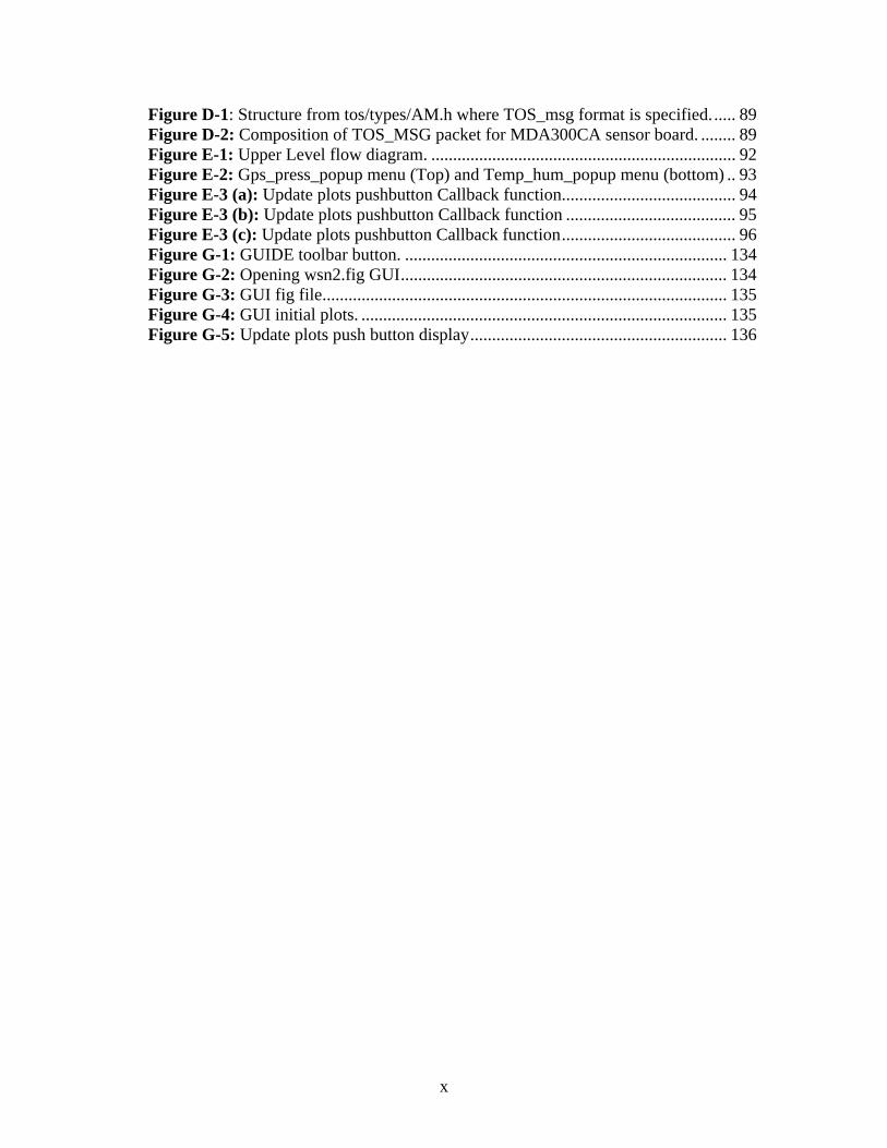
Figure D-1: Structure from tos/types/AM.h where TOS_msg format is specified...... 89 Figure D-2: Composition of TOS_MSG packet for MDA300CA sensor board. ........ 89 Figure E-1: Upper Level flow diagram. ...................................................................... 92 Figure E-2: Gps_press_popup menu (Top) and Temp_hum_popup menu (bottom) .. 93 Figure E-3 (a): Update plots pushbutton Callback function........................................ 94 Figure E-3 (b): Update plots pushbutton Callback function ....................................... 95 Figure E-3 (c): Update plots pushbutton Callback function........................................ 96 Figure G-1: GUIDE toolbar button. .......................................................................... 134 Figure G-2: Opening wsn2.fig GUI........................................................................... 134 Figure G-3: GUI fig file............................................................................................. 135 Figure G-4: GUI initial plots. .................................................................................... 135 Figure G-5: Update plots push button display........................................................... 136

1
Chapter 1 Introduction
Wireless Sensor Networks (WSN) can be deployed where the measurement of
environment parameters is dangerous or difficult to access. For example applications
such as sensing a building integrity or structural vibrations during an earthquake, the
stress of an airplane’s wings, are some of the applications where WSN promise to change
how researchers gather their data.
A WSN is composed of various sensor modules attached to radio modules
(motes). They can be deployed in areas where the parameters of interest need to be
measured. Their computational capability is limited, so the data is transmitted at low
speeds; few bytes per hour at most. Motes transmit the data from mote to mote in an ad-
hoc way back to a base station where the data is stored, processed and displayed. The
radio motes require minimal attention if they are setup in appropriate locations and with
the appropriate housings which protect the electronic components. Their power source, a
pair of AA batteries, lasts an average of one year assuming transmission is not constant
[5]. The versatility in which WSN can be applied to any system(s) and their flexibility
require extensive research and development.
This thesis demonstrates, via a proof of concept, the usefulness of WSN by
integrating five main application sensors and a GPS module into a graphical user
interface. It also pioneers, along with other theses and four senior projects, the studies of
wireless sensor networks at Cal Poly San Luis Obispo; it provides a report where it
unifies four senior projects where new students can follow to get a jump-start in the
studies of WSN applications.

2
This report is organized as follows: Chapter 2 is dedicated to the background of
Wireless Sensor Networks, as well as how and where it started. It gives examples of
current work done in WSN and the motivation for this thesis project. Chapter 3 describes
the hardware that was used; Crossbow technology. In Chapter 4, the uses of different
software with motes in this project are introduced. The system sensor integration and
Graphical User Interface is treated in Chapter 5. Chapter 6 is dedicated to the results of
testing the system. Chapter 7 concludes the project and suggests future work, lessons
learned and suggestions. The Appendices provide software code and extra information
needed for this project.

3
Chapter 2 Background
2.1 Wireless Sensor Networks Overview
Twenty years ago most of the efforts were put into the design of computer
architecture and CPU design [8]. In the 1990’s the focus was to build around highly
integrated microcontrollers. In the years after 2000, the software for embedded systems
took more importance and operating systems provided a high level of design abstractions
as mentioned by Bruce Heminway, Waylon Brunette, Tom Anderl and Gaetano Borrielo
of the University of Washington which are integrating WSN into their curriculum [8].
Most recently the wireless communication ability has made more complex the embedded
applications world by leading to the development of sensor networks [8]. Also, in the past
decade, most of the research has been focused to increase the practical data bandwidth of
wireless communications, for example: the development of WiFi for ‘hot spots’ for
public wireless Internet access which requires a high bandwidth to transmit the increasing
demand for media to the user. However, there are applications that do not require a
bandwidth as high as tens of megabit per second. These applications only need a few
bytes per day. Most of these low-data-rate applications involve some sort of sensing and
may require each node to work actively or to coordinate with each other to some extent.
These kinds of wireless communication networks are called wireless sensor networks.
A node or mote of a wireless sensor network usually consists of the following:
various kinds of sensors, microprocessors, and wireless communication hardware. The
following are some examples of wireless sensor networks;

4
Precision-Farming Vineyards: there are about 20 types of microclimates and
several types of soils within a 46 acre area; matching the right type of grapes with the
right type of land is very difficult, Don King a vineyard farmer explains in a discovery
channel video [37]. Every mismatch in type of grapes and type of soil costs about
$20000 in loss per acre of land [37]. The motes help to study the microclimates so
farmers can take care of individual sections. This is called precision farming; an
emerging new approach to increase the productivity of crops, in this case vineyards. Don
and his brother deployed 65 motes over one acre of vineyards which makes this project,
the largest in the world to use wireless sensor networks technology. At the current
moment the motes only measure temperature but in the future the farmers plan to use
them to monitor the sections of vineyard with mildew and for irrigation. Large farms and
ranches may receive rain unevenly. Wireless sensors detect soil moisture to let the
irrigation system know where to irrigate more and when to irrigate less. Intel believes the
sensors will help aid the third world people to understand the microclimates of their
agricultural industry to maximize their crop yield and improve profits [37].
Industrial Control and Monitoring: Wireless sensors can be used to monitor the
state of machinery or to measure environmental parameters in harsh environments. Cost
can be reduced by not using wiring connections to the sensing devices.
Building Monitoring: Intel expects motes to be as tiny as a rice grain and as cheap
as one dollar in five years making wireless sensor applications soar [37]. With improving
technology, WSN can be deployed in buildings to monitor and control air conditioning.
This will help to eliminate any hot or cold spots for a more effective air conditioning. A

5
building’s illumination can be controlled and balanced in a similar way as the
temperature.
Patient Monitoring: The United States is struggling to give health support to 34
million senior citizens today [38]. This number is expected to increase in the next decade
to 76 million baby boomers [38]. That is why the focus of health care should shift from
treatment to prevention at home and by creating a digital home with wireless sensor
networks would help prevent medical issues. Wireless sensors can be used to monitor the
status of patients, logging information about the patients’ whereabouts and normal duties.
With the information the computers can monitor their health status while they live
normally in their own place. Once it detects an abnormal situation, the computer can alert
their family or medical personnel immediately. As mentioned in an article in intel’s
website “Older adults will be able to access these applications through whatever
interfaces are most familiar to them, from phones to PCs to televisions; they will not have
to learn new technology.”[38].
2.2 Motivation
As with any state of the art technology, there is no point of reference or guidance to
follow. Two graduate and four undergraduate students, started doing research on WSN in
January 2005. Our objective was unknown at the time. Dr. Harris, our advisor, suggested
reviewing the Tinyos.net online tutorials so we could familiarize ourselves with the
hardware and software we were about to research. By the fifth week we should have a
well-defined topic to do research on. The objective was to find an application for
Wireless Sensor Networks.
6
Motivation to find an application in agriculture at Cal Poly, San Luis Obispo came after
reading an online environmental application at Great Duck Island Maine, where WSN
was used to monitor the microclimates in and around nesting burrows used by the
Leach’s Storm Petrel [31].
Dr. Harris referred us to Dr. Dietterick, Cal Poly’s Swanton Pacific Ranch
Director; we could find an environmental application for the ranch. Another possible
application at Cal Poly would be at the greenhouses. The following two sections provide
more information on the two possible applications.
2.2.1 Swanton Pacific Ranch
Swanton Pacific Ranch (SPR) was donated to Cal Poly in the will of Al Smith
who died December 18, 1993. He was a Cal Poly Alumni who graduated in the 1940's
with a degree in Crop Science [22]. SPR consists of a diverse landscape overlooking the
Pacific Ocean. It is located 12 miles north of Santa Cruz CA. The 3200 acres make up
part of an original Mexican land grant originally called “Rancho Agua Puerca y las
Trancas.” At a meeting with the ranch director, Dr. Dietterick, we discussed possible
WSN applications at the ranch. Our objective was to demonstrate the potential of
Wireless Sensor Networks by creating a prototype project where future Cal Poly students
would be able to add research and improve the application.
Wireless sensors can be used at the ranch to measure:
• Sound (microphone integrated)
• Light
• Temperature

7
• 2-axis Accelerometer
• 2-axis Magnetometer
Even though the communication radius is claimed by crossbow technologies to be
about 500ft transmission at their maximum transmission power (5dBm) 1 meter off the
ground, their range is limited by the amount of motes in the network [2]. Motes can be
powered by two AA batteries, which last approximately 1 year depending on the data
transfer rate and power settings [2]. Please refer to the table 2.1 below.
Solar power is another option, but it is more expensive. Ideally, with enough
motes scattered along the creek with approximately 400ft of distance between them, the
network of motes would gather all the desired data which would be passed from mote to
mote until they can reach their final destination; a central computer with a graphical user
interface or GUI.
Table 2.1: Current drained by MICA2 motes at different Output Power settings. MICA2 900Mhz Pout Iq (mA) -20dBm 8.6 -5dBm 13.8 0dBm 16.5 5dBm 25.4 Since Swanton Pacific Ranch consists of 3200 acres and contains approximately 3 miles
of creek, it would take approximately 40 motes to cover the length of the creek.
The price for motes is:
MDA300CA = $250 MTS420CA - GPS WEATHER BOARD = $375 MTS310CA MAG-ACCEL SENSOR = $210 MPR400CB MICA2, 900MHz =$125 MMA410CA - WHIP ANT 433MHz=$14 HOUSING = $49
8
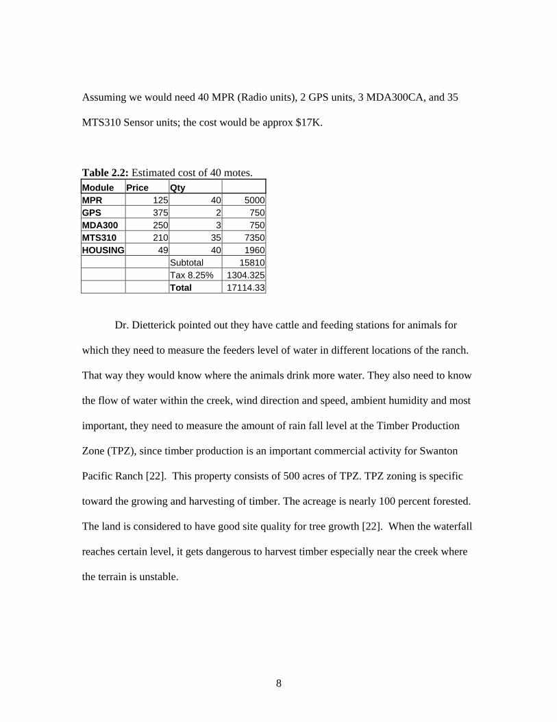
Assuming we would need 40 MPR (Radio units), 2 GPS units, 3 MDA300CA, and 35
MTS310 Sensor units; the cost would be approx $17K.
Table 2.2: Estimated cost of 40 motes. Module Price Qty MPR 125 40 5000GPS 375 2 750MDA300 250 3 750MTS310 210 35 7350HOUSING 49 40 1960 Subtotal 15810 Tax 8.25% 1304.325 Total 17114.33
Dr. Dietterick pointed out they have cattle and feeding stations for animals for
which they need to measure the feeders level of water in different locations of the ranch.
That way they would know where the animals drink more water. They also need to know
the flow of water within the creek, wind direction and speed, ambient humidity and most
important, they need to measure the amount of rain fall level at the Timber Production
Zone (TPZ), since timber production is an important commercial activity for Swanton
Pacific Ranch [22]. This property consists of 500 acres of TPZ. TPZ zoning is specific
toward the growing and harvesting of timber. The acreage is nearly 100 percent forested.
The land is considered to have good site quality for tree growth [22]. When the waterfall
reaches certain level, it gets dangerous to harvest timber especially near the creek where
the terrain is unstable.

9
2.2.2 Cal Poly Greenhouses
The Cal Poly Greenhouses were the possible second application of WSN that we
considered, and as Virginia Walter explains in an email to Dr. Harris, WSN can be
applied in the following areas:
1. To measure the electrical conductivity and pH of irrigation water and
drainage water and of the soil solution.
2. To measure both irrigation and drainage quantity and temperature. Number
of times and length of times irrigation systems came on.
3. To measure soil temperature.
4. To measure the amount of carbon dioxide content of air over time.
5. To measure the leaf temperature.
6. To measure photon flux of light.
7. To measure light quality, quantity, and duration.
8. To measure nutrient content of fertility system.
The complete list of possible applications to a greenhouse environment as mentioned by
Virginia Walter is included in appendix C.
2.3 System Requirements for Proof of Concept Design.
Thus our project was clear. The demonstration would include a sensor board attached to a
radio mote measuring the following parameters:

10
• Wind speed and direction
• Rain fall level
• Temperature
• Water level
• Humidity
• GPS
All this data should be gathered wirelessly by the Base station computer, saved into a file
for later used by MATLAB to plot the data vs. time. Please see figure 2.1 for the overall
tentative hardware setup. We needed to create a demonstration of the setup mentioned
above and a graphical user interface or GUI to display the data correctly.
After the project was defined, I was to oversee four senior projects from four
undergraduate students. The work mentioned above shall be divided among us as
follows:
Student #1: Rain Gauge
Student #2: Wind Speed and Direction (anemometer)
Student #3: Humidity, temperature and Barometric pressure
Student #4: GPS Module
By using the information provided by the undergrad students, like conversion formulas
and sensor connections, a GUI display for the sensors and GPS shall be developed.
The following chapters are divided as follows:
Chapter 3 will give an overview of the capabilities/weaknesses and features of the
11
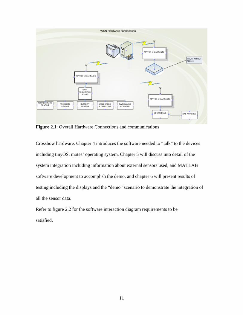
Figure 2.1: Overall Hardware Connections and communications
Crossbow hardware. Chapter 4 introduces the software needed to “talk” to the devices
including tinyOS; motes’ operating system. Chapter 5 will discuss into detail of the
system integration including information about external sensors used, and MATLAB
software development to accomplish the demo, and chapter 6 will present results of
testing including the displays and the “demo” scenario to demonstrate the integration of
all the sensor data.
Refer to figure 2.2 for the software interaction diagram requirements to be
satisfied.
12
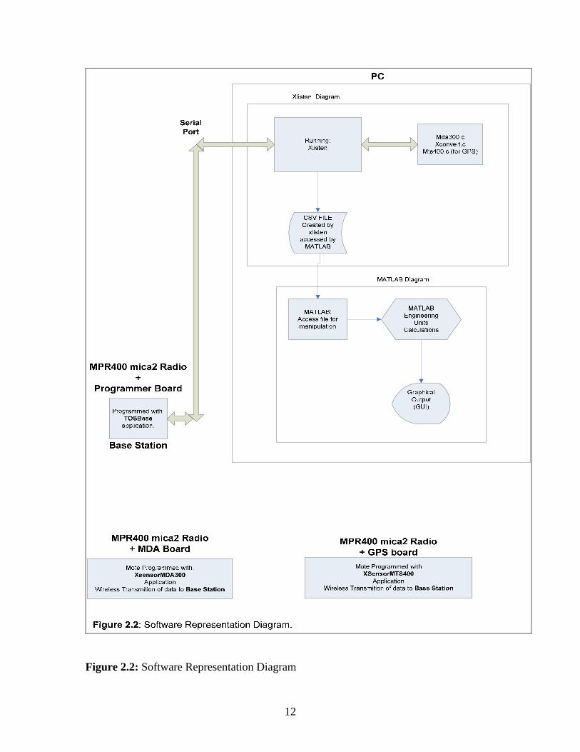
Figure 2.2: Software Representation Diagram

13
In figure 2.2, the hardware is labeled outside the boxes, and the content of each box
represents the software programmed/used for that hardware.
2.3.1 LIST OF PROJECT REQUIREMENTS
1. Shall integrate six different sensor data:
A. Wind direction
B. Wind speed
C. Relative humidity
D. Pressure
E. Rain gauge
F. Temperature
G. GPS
2. A base station computer should gather sensor data.
3. To develop a methodical way of changing and adding new sensors to the system.
4. Shall develop a way of adding or modifying the sensor engineering conversion formulas.
5. There shall be one display for the GUI with four display axes.
i. Shall display rain gauge readings vs. time
ii. Shall display either
GPS (Latitude Longitude) or
Pressure (mBar)
iii. Shall display wind speed and direction in one plot.

14
iv. Shall display either
Relative Humidity (%Hum) or
Temperature (F)
2.3.2 SOFTWARE REQUIREMENTS
• MATLAB version 7.2.0.232 (R2006a)
• TinyOS version 1.1.7
• Microsoft Excel 2000 or newer
• Microsoft Streets and trips
2.3.3 HARDWARE REQUIREMENTS • A PC with an available serial port or
• A laptop with an available serial port or an USB to Serial cable converter
• 1 Crossbow MIB510 programmer board
• 3 Crossbow MPR400CB Mica2 motes
• 1 Crossbow MDA300CA data acquisition board
• 1 Crossbow MTS420CA GPS module
• 1 ZANTEN0203 GPS antenna for MTS420CA
• 4 AA batteries
• 1 Davis part # 7911 anemometer (wind and speed sensor)
• 1 Davis part # 7852 Rain Gauge
• 1 Humirel model HM1500 Humidity sensor
• 1 Motorola MPXA6115A6U-ND Pressure Sensor
• 1 Thermistor 10K ohm NTC digikey part # BC1489-ND

15
• Assorted resistors

16
Chapter 3 Hardware Overview
The hardware available to us was from crossbow technologies. Crossbow Technology at
as of February 7th 2006, claimed to be the global leader in wireless sensor supplier,
shipping five times more sensors than their closest competitor [2].
The following companies are among the most important developers of Wireless Sensor
Network hardware [1].
• Digital Sun’s S.Sense: (www.digitalsun.com) A soil moisture sensor system to keep
grass green while saving water
• Dust Inc.: (www.dust-inc.com):Reliable Low Power Wireless Networks
• Crossbow: (www.xbow.com) : A Clear and Compelling Vision of Sensor Technology
• Ember: (www.ember.com/company/overview.html) Reliable, Secure, Easy-to-Use
Embedded Wireless Networking
• Sensicast: (www.sensicast.com) Providing wireless sensor network solutions
• Sensit: (www.sensit.com) The most highly preferred wind eroding mass sensor erosion
worldwide
Source: www.tinyos.net
Each mote is composed of the following components [2].
• Microprocessor or micro controller,
• Wireless Radio
• Sensor board
• Power Supply
17
The following sections describe the components that were used from crossbow
technology.
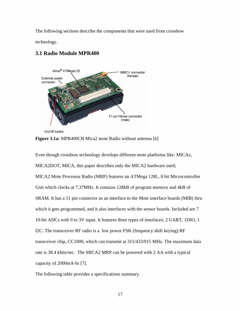
3.1 Radio Module MPR400
Figure 3.1a: MPR400CB Mica2 mote Radio without antenna [6] Even though crossbow technology develops different mote platforms like: MICAz,
MICA2DOT, MICA, this paper describes only the MICA2 hardware used;
MICA2 Mote Processor Radio (MRP) features an ATMega 128L, 8 bit Microcontroller
Unit which clocks at 7.37MHz. It contains 128kB of program memory and 4kB of
SRAM. It has a 51 pin connector as an interface to the Mote interface boards (MIB) thru
which it gets programmed, and it also interfaces with the sensor boards. Included are 7
10-bit ADCs with 0 to 3V input. It features three types of interfaces; 2 UART, 1DIO, 1
I2C. The transceiver RF radio is a low power FSK (frequency shift keying) RF
transceiver chip, CC1000, which can transmit at 315/433/915 MHz. The maximum data
rate is 38.4 kbits/sec. The MICA2 MRP can be powered with 2 AA with a typical
capacity of 2000mA-hr [7].
The following table provides a specifications summary.
18
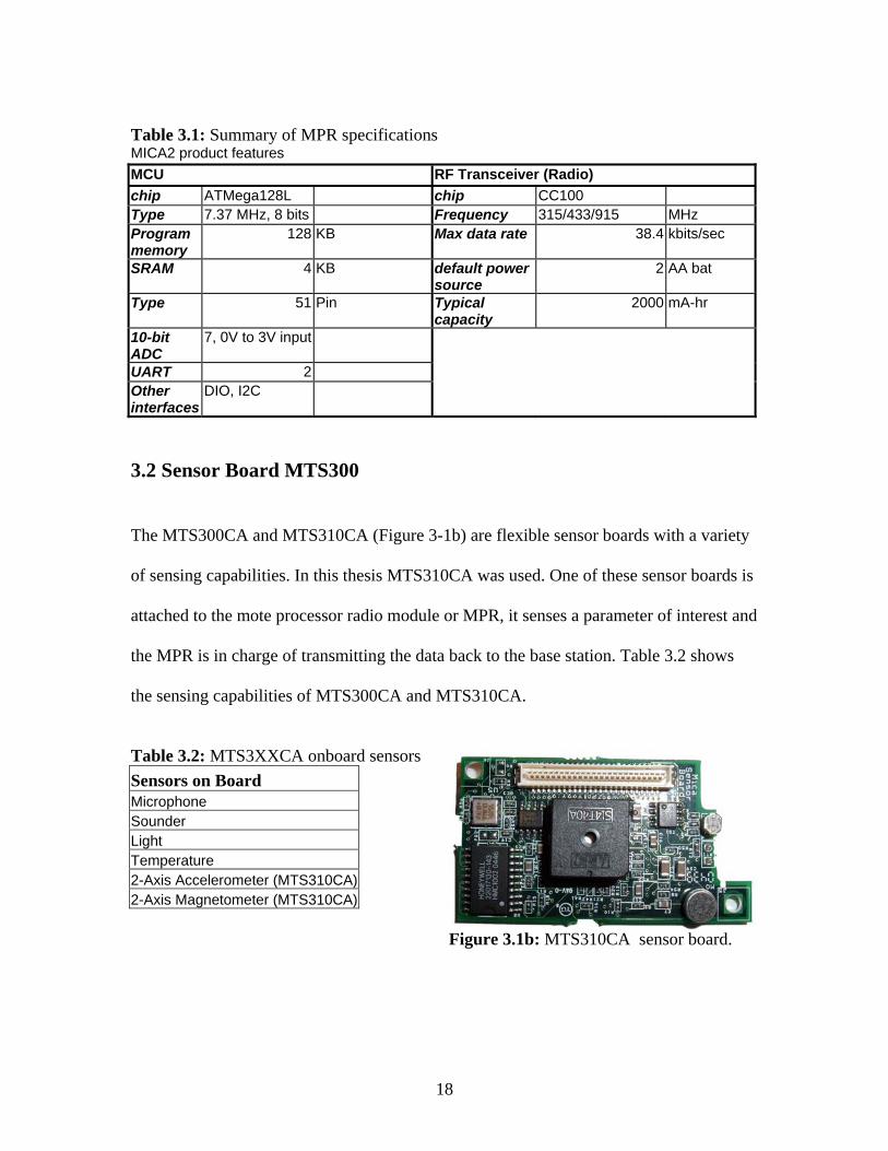
Table 3.1: Summary of MPR specifications MICA2 product features MCU RF Transceiver (Radio) chip ATMega128L chip CC100 Type 7.37 MHz, 8 bits Frequency 315/433/915 MHz Program memory
128 KB Max data rate 38.4 kbits/sec
SRAM 4 KB default power source
2 AA bat
Type 51 Pin Typical capacity
2000 mA-hr
10-bit ADC
7, 0V to 3V input
UART 2 Other interfaces
DIO, I2C
3.2 Sensor Board MTS300
The MTS300CA and MTS310CA (Figure 3-1b) are flexible sensor boards with a variety
of sensing capabilities. In this thesis MTS310CA was used. One of these sensor boards is
attached to the mote processor radio module or MPR, it senses a parameter of interest and
the MPR is in charge of transmitting the data back to the base station. Table 3.2 shows
the sensing capabilities of MTS300CA and MTS310CA.
Table 3.2: MTS3XXCA onboard sensors Sensors on Board Microphone Sounder Light Temperature 2-Axis Accelerometer (MTS310CA)2-Axis Magnetometer (MTS310CA) Figure 3.1b: MTS310CA sensor board.
19
Microphone: The microphone circuit has two principal uses: Its first is for acoustic
ranging and second is for general acoustic recording and measurement [6].
Sounder: self explanatory, sound frequency is 4kHz fixed frequency piezoelectric
resonator.
Light and Temperature: The MTS sensor board can measure light and temperature. the
two sensors share the same Analog to Digital Channel (ADC1). When accessing light and
temperature, it should not be done at the same time.
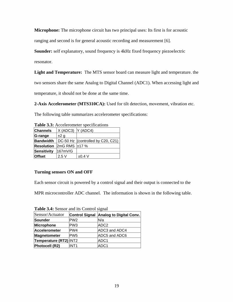
2-Axis Accelerometer (MTS310CA): Used for tilt detection, movement, vibration etc.
The following table summarizes accelerometer specifications:
Table 3.3: Accelerometer specifications Channels X (ADC3) Y (ADC4) G-range ±2 g Bandwidth DC-50 Hz (controlled by C20, C21)Resolution 2mG RMS ±17 % Sensitivity 167mV/G Offset 2.5 V ±0.4 V Turning sensors ON and OFF
Each sensor circuit is powered by a control signal and their output is connected to the
MPR microcontroller ADC channel. The information is shown in the following table.
Table 3.4: Sensor and its Control signal Sensor/Actuator Control Signal Analog to Digital Conv.Sounder PW2 N/a Microphone PW3 ADC2 Accelerometer PW4 ADC3 and ADC4 Magnetometer PW5 ADC5 and ADC6 Temperature (RT2) INT2 ADC1 Photocell (R2) INT1 ADC1

20
More information about MTS310CA can be found in MTS/MDA sensor board user’s
manual [6].
3.3 Serial Programmer MIB510
The Serial programmer or base station is connected to the receiving data PC. It serves to
initially program the MPR boards and it is used to receive all the data from motes for
later redirection thru the interface RS-232. The MIB510 interface board was used which
is a multi-purpose interface board used with MICA2, MICA, MICAz, and MICA2DOT
from crossbow family of products. A 5V 1.5A power adapter or two 1.5V AA batteries
power the programmer board. It is recommended to use the power outlet when
programming other boards since the flash needs a fully charged battery to be
programmed. The programmer can be damaged if both power sources are used at the
same time [5].
If we were to measure water pressure, wind speed, rain fall, or any parameter which the
simple contact of our sensor board and the environment could affect the performance or
integrity of our sensors, we need to add external sensors to our available hardware. As we
previously mentioned, the sensor board available to us, the MTS 310CA doesn’t meet our
requirements. So the question arises: Can we connect external sensors to a Mica Mica2
Board? And the answer: quote “while it is possible to connect directly to an MPR
(MICA2 or MICA2DOT) board, it is not recommended”[2]. After all of us, four
undergraduate students and a graduate student, researched for a possible data acquisition
board to use with the motes, we came out with the following options.
• MICA2: MTS101
• MICA2: MDA300CA
21
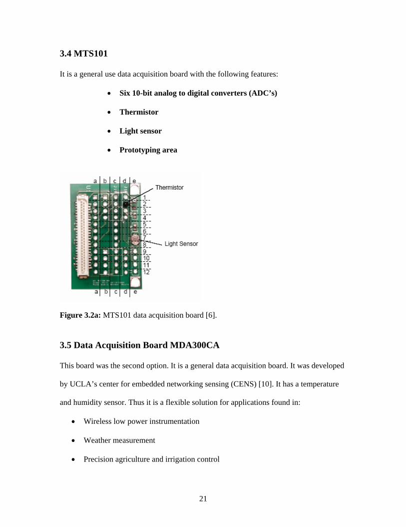
3.4 MTS101
It is a general use data acquisition board with the following features:
• Six 10-bit analog to digital converters (ADC’s)
• Thermistor
• Light sensor
• Prototyping area
Figure 3.2a: MTS101 data acquisition board [6]. 3.5 Data Acquisition Board MDA300CA
This board was the second option. It is a general data acquisition board. It was developed
by UCLA’s center for embedded networking sensing (CENS) [10]. It has a temperature
and humidity sensor. Thus it is a flexible solution for applications found in:
• Wireless low power instrumentation
• Weather measurement
• Precision agriculture and irrigation control
22
• Habitat monitoring
• Soil analysis
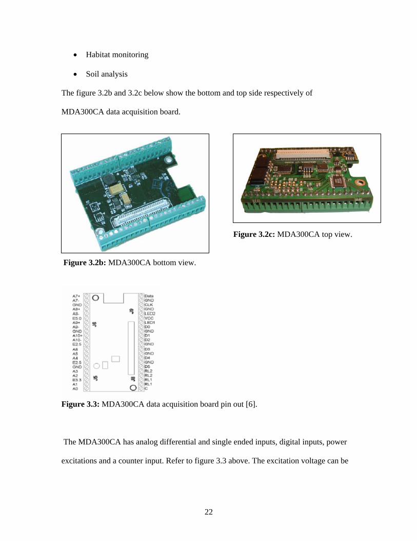
The figure 3.2b and 3.2c below show the bottom and top side respectively of
MDA300CA data acquisition board.
Figure 3.2c: MDA300CA top view. Figure 3.2b: MDA300CA bottom view.
Figure 3.3: MDA300CA data acquisition board pin out [6].
The MDA300CA has analog differential and single ended inputs, digital inputs, power
excitations and a counter input. Refer to figure 3.3 above. The excitation voltage can be
23
used to power sensors, which supply voltage only when the sensor is called for
measurement, thus saving battery power. Please see the following summary.
• 7 single-ended or 3 differential ADC channels
• 4 precise differential ADC channels
• 6 digital I/O channels with event detection interrupt
• 64K EEPROM for on-board sensor calibration data
• 2 relay channels-one normally open and one normally closed
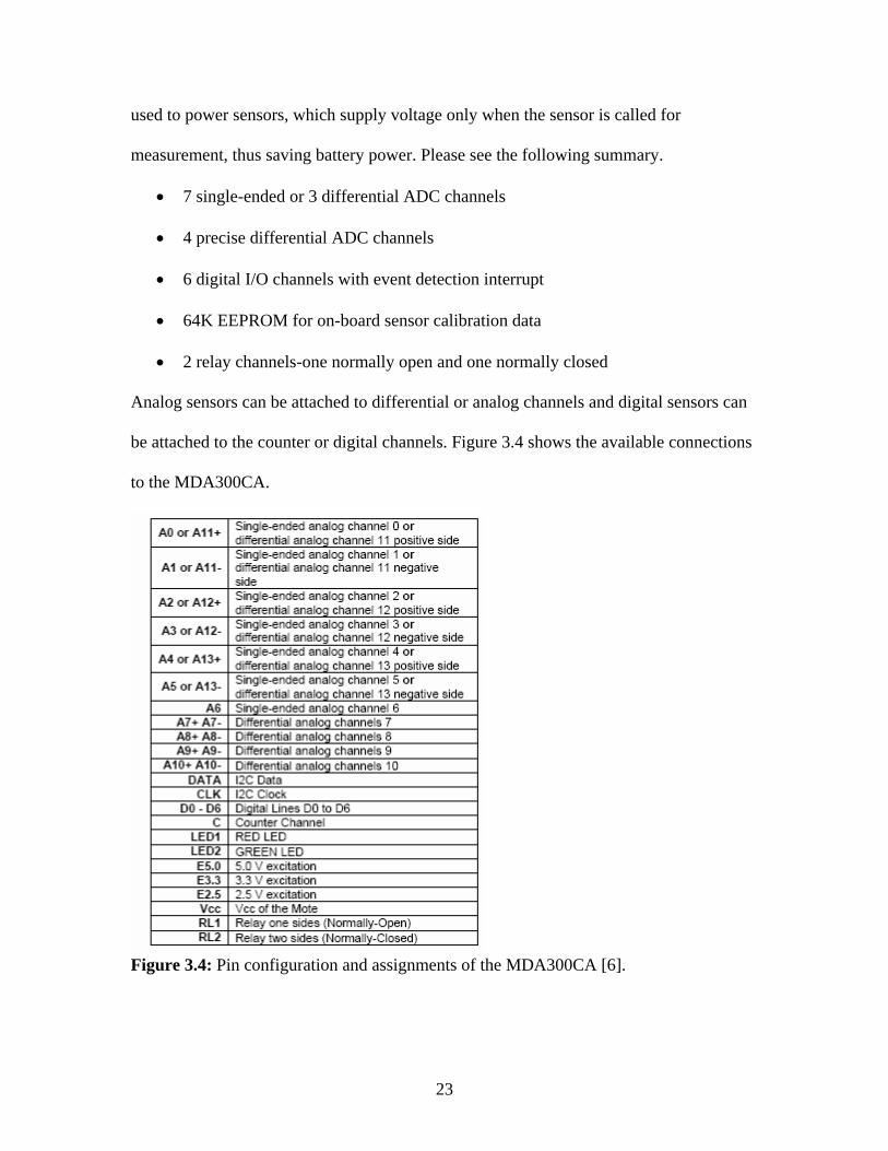
Analog sensors can be attached to differential or analog channels and digital sensors can
be attached to the counter or digital channels. Figure 3.4 shows the available connections
to the MDA300CA.
Figure 3.4: Pin configuration and assignments of the MDA300CA [6].
24
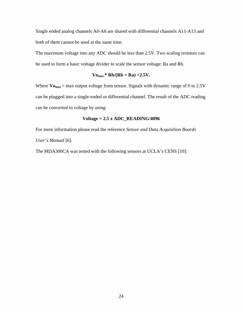
Single ended analog channels A0-A6 are shared with differential channels A11-A13 and
both of them cannot be used at the same time.
The maximum voltage into any ADC should be less than 2.5V. Two scaling resistors can
be used to form a basic voltage divider to scale the sensor voltage: Ra and Rb.
Vomax * Rb/(Rb + Ra) <2.5V.
Where Vomax = max output voltage from sensor. Signals with dynamic range of 0 to 2.5V
can be plugged into a single-ended or differential channel. The result of the ADC reading
can be converted to voltage by using:
Voltage = 2.5 x ADC_READING/4096
For more information please read the reference Sensor and Data Acquisition Boards
User’s Manual [6].
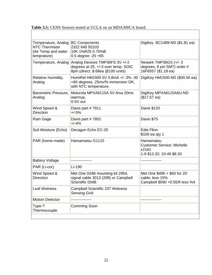
The MDA300CA was tested with the following sensors at UCLA’s CENS [10]:
25
Table 3.5: CENS Sensors tested at UCLA on an MDA300CA board. We have tested the board with couple of sensors.The list of the sensors tested so far are:
Temperature, Analog NTC Thermistor (Air Temp and water temprature)
BC Components 2322 640 55103 10K 1%R25 0.75%B 0.5 degree -25 +65
Digikey BC1489-ND ($1.81 ea)
Temperature, Analog Analog Devices TMP36FS 3V +/-2 degrees at 25, +/-3 over temp, SOIC 8pin (direct: $.68ea @100 units)
Newark TMP36GS (+/- 3 degrees, 8 pin SMT) order # 16F6557 ($1.18 ea)
Relative Humidity, Analog
HumiRel HM1500 5V 0.8mA +/- 3% -30 +60 degrees, 25mv/% immersion OK, with NTC temperature.
DigiKey HM1500-ND ($30.50 ea)
Barometric Pressure, Analog
Motorola MPXA6115A 5V 6ma 20ms warmup, 0-5V out
DigiKey MPXA6115A6U-ND ($17.57 ea)
Wind Speed & Direction
Davis part # 7911 +/-5%
Davis $120
Rain Gage Davis part # 7852 +/-4%
Davis $75
Soil Moisture (Echo) Decagon Echo EC-20 Edie Flinn $100 ea qty 1
PAR (home-made) Hamamatsu G1115 Hamamatsu Customer Service: Michelle x2161 1-9 $13.32; 10-49 $8.33
Battery Voltage ---------------- ----------------
PAR (Li-cor) LI-190
Wind Speed & Direction
Met One 034B mounting kit 2954, signal cable 3013 (20ft) or Campbell Scientific 034B
Met One $495 + $60 for 20’ cable; less 15% Campbell $590 +0.55/ft less %4
Leaf Wetness Campbell Scientific 237 Wetness Sensing Grid
Motion Detector ---------------- ----------------
Type-T Thermocouple
Comming Soon
26
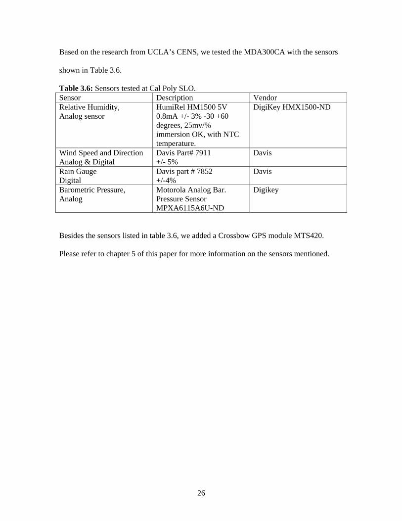
Based on the research from UCLA’s CENS, we tested the MDA300CA with the sensors
shown in Table 3.6.
Table 3.6: Sensors tested at Cal Poly SLO. Sensor Description Vendor Relative Humidity, Analog sensor
HumiRel HM1500 5V 0.8mA +/- 3% -30 +60 degrees, 25mv/% immersion OK, with NTC temperature.
DigiKey HMX1500-ND
Wind Speed and Direction Analog & Digital
Davis Part# 7911 +/- 5%
Davis
Rain Gauge Digital
Davis part # 7852 +/-4%
Davis
Barometric Pressure, Analog
Motorola Analog Bar. Pressure Sensor MPXA6115A6U-ND
Digikey
Besides the sensors listed in table 3.6, we added a Crossbow GPS module MTS420.
Please refer to chapter 5 of this paper for more information on the sensors mentioned.
27
Chapter 4 Software Overview This chapter describes the software needed including MATLAB, tinyOS and the
modifications made to four existing code files. It describes the main idea of the software
integration lays out the background for the system integration and the conversion formula
editing and creation. It also describes the relationship between Xlisten and MATLAB,
the logged csv files, sample output data and provides an example problem with solution.
4.1 TinyOS
TinyOS is an open source operating system originally designed at University of
California Berkeley. It is specially designed for resource constrained low power, low
memory processors. TinyOS is the standard for wireless sensor networking. It has
created a broad user community with thousands of developers. TinyOS is an object –
oriented, event driven operating system. TinyOS supports microprocessors with 8-bit
architectures with 2KB of RAM to 32-bit processors with 32MB of RAM or more [33]. It
features a component-based architecture, which enables reusability of code for user
applications, and rapid “wiring” of components to create an application. TinyOS event-
driven execution enables the user to create custom code to handle the unpredictability of
physical world interfaces. TinyOs is continuously used and code its being contributed by
a large community of developers to its source forge site [1].
28
4.2 Xlisten
Xlisten is a User Interface that serves as a tool to test the functionality of available data
acquisition boards (DAQs). It displays the DAQ’s output in a Cygwin window. Xlisten
needs a DAQ board application and a driver, which can be modified to develop custom
applications and to meet data logging needs. The board drivers are located at opt/tinyos-
1.x/contrib/xbow/tos/sensorboards, and the XSensor Applications are located at:
opt/tinyos-1.x/contrib/xbow/apps/.
Xlisten can be used to test motes:
1. Over the UART
2. Over the RF
For more information refer to the Getting Started Guide Chapter [5].
For a single mote configuration, the mote must be programmed with a XSensorMXX###
application and plugged into the MIB510. The mote will stream packets over the UART
or the radio.
For the network of motes configuration, a base station mote needs to be programmed
with TOSBase and plugged into the MIB510. All other motes need to be installed with
an XSensorMXX## application and put within range of the base station or a valid multi-
hop peer. Xlisten must then be run with the -w flag to properly parse the wireless
29
packets. Please look at Appendix A for instructions on how to program a mote, and
Appendix B for a more complete discussion of the Xlisten display options. Take care to
program all the motes to the same frequency and group id.
Xlisten is a program included with TinyOS installation. The one used in this thesis, came
with TinyOS installation upgrade 1.1.7. It can be found in the following folder:
c:\tinyos\cygwin\opt\tinyos-1.x\contrib\xbow\tools\src\xlisten
Originally, this program was used to test if the different sensor boards are functioning
correctly. For example, the following boards can be tested with Xlisten:
Mda300, mda500, mep401, mep500, mts101, 300,400 & 510.
Using the original version of Xlisten, different viewing options can be specified at the
cygwin command prompt. For example running Xlisten with the parsed mode (-p flag)
as follows:
$ ./xlisten –p –s=com4
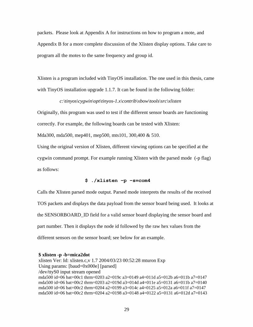
Calls the Xlisten parsed mode output. Parsed mode interprets the results of the received
TOS packets and displays the data payload from the sensor board being used. It looks at
the SENSORBOARD_ID field for a valid sensor board displaying the sensor board and
part number. Then it displays the node id followed by the raw hex values from the
different sensors on the sensor board; see below for an example.
$ xlisten -p -b=mica2dot xlisten Ver: Id: xlisten.c,v 1.7 2004/03/23 00:52:28 mturon Exp Using params: [baud=0x000e] [parsed] /dev/ttyS0 input stream opened mda500 id=06 bat=00c1 thrm=0203 a2=019c a3=0149 a4=011d a5=012b a6=011b a7=0147 mda500 id=06 bat=00c2 thrm=0203 a2=019d a3=014d a4=011e a5=0131 a6=011b a7=0140 mda500 id=06 bat=00c2 thrm=0204 a2=0199 a3=014c a4=0125 a5=012a a6=011f a7=0147 mda500 id=06 bat=00c2 thrm=0204 a2=0198 a3=0148 a4=0122 a5=0131 a6=012d a7=0143
30
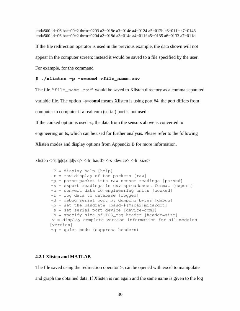
mda500 id=06 bat=00c2 thrm=0203 a2=019e a3=014e a4=0124 a5=012b a6=011c a7=0143 mda500 id=06 bat=00c2 thrm=0204 a2=019d a3=014c a4=011f a5=0135 a6=0133 a7=011d If the file redirection operator is used in the previous example, the data shown will not
appear in the computer screen; instead it would be saved to a file specified by the user.
For example, for the command
$ ./xlisten –p –s=com4 >file_name.csv
The file “file_name.csv” would be saved to Xlisten directory as a comma separated
variable file. The option -s=com4 means Xlisten is using port #4. the port differs from
computer to computer if a real com (serial) port is not used.
If the cooked option is used -c, the data from the sensors above is converted to
engineering units, which can be used for further analysis. Please refer to the following
Xlisten modes and display options from Appendix B for more information.
xlisten <-?|r|p|c|x|l|d|v|q> <-b=baud> <-s=device> <-h=size> -? = display help [help] -r = raw display of tos packets [raw] -p = parse packet into raw sensor readings [parsed] -x = export readings in csv spreadsheet format [export] -c = convert data to engineering units [cooked] -l = log data to database [logged] -d = debug serial port by dumping bytes [debug] -b = set the baudrate [baud=#|mica2|mica2dot] -s = set serial port device [device=com1] -h = specify size of TOS_msg header [header=size]
-v = display complete version information for all modules [version]
-q = quiet mode (suppress headers)
4.2.1 Xlisten and MATLAB
The file saved using the redirection operator >, can be opened with excel to manipulate
and graph the obtained data. If Xlisten is run again and the same name is given to the log
31
file, the file ‘file_name.csv’ is overwritten by the new data values by Xlisten. It is
not possible to graph the data more than once without having to manually create the
graphs, and it is not possible without the need of an external program to manipulate the
data file to display the graphs. Such a program should have I/O file manipulation, as
well as graphing capabilities. MATLAB and LAB VIEW are two programs that we had
access at school. The idea is to use MATLAB to create a GUI with displays (graphs) of
all the sensors that could be updated more than once at a single click of a button by the
user.
4.2.2 Accessing logged files with MATLAB
MATLAB has several commands that can read csv (comma separated variable) files,
which can be used to read and plot data; For example: csvread. In order to read the
data from the csv file using MATLAB, the data in each cell should only contain either
numerical data or characters. In other words, to use csvread, each cell should contain
only numbers since this command reads numeric data only. There are two approaches to
solve this problem.
1. The first option would be to modify the file ‘file_name.csv’ using
MATLAB after it is saved by Xlisten.
2. The second option would be to modify Xlisten itself to eliminate all the extra
characters and write only comma separated numerical values to the log file
‘file_name.csv’.
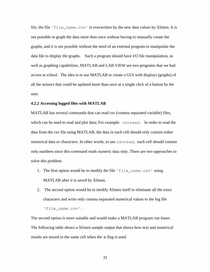
The second option is more suitable and would make a MATLAB program run faster.
The following table shows a Xlisten sample output that shows how text and numerical
results are mixed in the same cell when the -c flag is used.
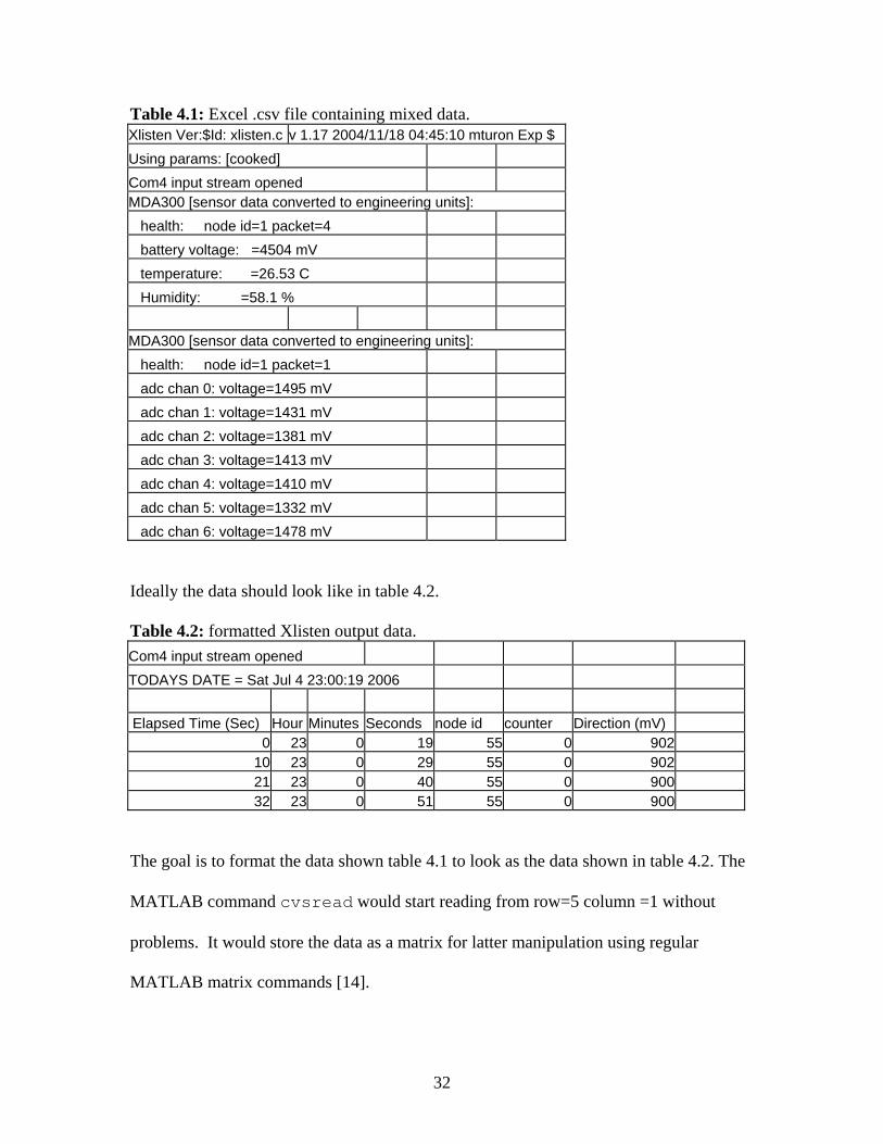
32
Table 4.1: Excel .csv file containing mixed data. Xlisten Ver:$Id: xlisten.c v 1.17 2004/11/18 04:45:10 mturon Exp $ Using params: [cooked] Com4 input stream opened MDA300 [sensor data converted to engineering units]: health: node id=1 packet=4 battery voltage: =4504 mV temperature: =26.53 C Humidity: =58.1 % MDA300 [sensor data converted to engineering units]: health: node id=1 packet=1 adc chan 0: voltage=1495 mV adc chan 1: voltage=1431 mV adc chan 2: voltage=1381 mV adc chan 3: voltage=1413 mV adc chan 4: voltage=1410 mV adc chan 5: voltage=1332 mV adc chan 6: voltage=1478 mV Ideally the data should look like in table 4.2.
Table 4.2: formatted Xlisten output data. Com4 input stream opened TODAYS DATE = Sat Jul 4 23:00:19 2006 Elapsed Time (Sec) Hour Minutes Seconds node id counter Direction (mV)
0 23 0 19 55 0 902 10 23 0 29 55 0 902 21 23 0 40 55 0 900 32 23 0 51 55 0 900
The goal is to format the data shown table 4.1 to look as the data shown in table 4.2. The
MATLAB command cvsread would start reading from row=5 column =1 without
problems. It would store the data as a matrix for latter manipulation using regular
MATLAB matrix commands [14].

33
4.3 Software Integration.
At this point, the student should have read tinyOS tutorial examples [36], Appendix A
Quick introduction, Reference Thesis [16], and should feel comfortable accessing
directories and programming existing applications. To get started Xlisten with the –x
flag, a XSensor application needs to be used and modified to log sensor data formatted as
in Table 4.2. The XSensor application for MDA300CA data acquisition board is called
XSensorMDA300M.nc. The output to excel formatting is done in the file mda300.c and
engineering conversion formulas for sensors are located in the file Xconvert.c.
Thus, the following files need to be modified
1 Xlisten.c
2 Mda300.c
3 XSensorMDA300M.nc
4 Xconvert.c
4.3.1 Modifications to Xlisten.c
As described in Section 4.2, depending on the arguments that are given to Xlisten when it
is run, the program parses the arguments and prints to the screen/file the corresponding
output to such argument. In Xlisten, the following line of code was commented out.
if (!g_params.bits.mode_quiet) {
// printf("xlisten Ver:%s\n", g_version);

34
If the quiet mode flag –p was not used, which almost always there is no need to use,
“xlisten Ver:” would be printed between packed readings. In this file almost all the output
options can be eliminated, but that would cut the functionality of the original program. So
only the absolute necessary changes were made, leaving code for new students to
reference and use their functions for other projects.
This project was concerned with only –x –c –p flags, and the –r (raw) flag was
eliminated it can be used as an input argument but it wouldn’t have any effect on the
output.
The fact that Xlisten does not support custom packet formats is a major setback, but
Xlisten is still very useful to understand how to develop new applications.
4.3.2 XSensorMDA300M.nc This file is the module of the MDA300 application called XSensorMDA300 located at c:/tinyos/cygwin/opt/tinyos-1.x/contrib/xbow/apps/XSensorMDA300.
This application should be programmed into the mote connected a MDA300CA sensor
board with external sensors connected to it. Refer to Figure 4.1 and 2.1 for the main flow
diagram after data is obtained and hardware overview respectively. XSensorMDA300
contains all the calls to the inputs to measure for the MDA300 sensors, the handling and
composition of packets, UART send, and RF send. This file is to be modified when more
external sensors are to be added. The commands to call an input to read are described in
the MDA300 datasheet [28]. To demonstrate their use, an example is provided below:
35
Problem:
A digital sensor needs to be connected and programmed to an MDA board. This sensor
will toggle logic hi and low every time a door is opened or closed respectively. It will
count the number of times the door is activated per hour. And such count is to be
included in a packet of any format and needs to be send along with other three channel
readings (the other channels are not relevant for this example).
Solution:
A MDA board features six digital channels 0-5. Choose an open channel, for example
CH5. Next assume the door activates a simple switch circuit. Refer to for rain gauge
schematic shown in Appendix J. When the door is closed the switch is closed. Since
digital channels have an internal pull-up resistor, the closing of the door will pull-down
the input voltage at digital CH5. A falling-edge trigger will detect an open-to-closed door
event, and a rising-edge trigger will detect a closed-to-open door event. Reading
reference [28], the following commands can be added to XSensorMDA300M.nc:
1 SAMP_TIME = 3600000; //1 HR INTERVAL 2 3 record[1] = call Sample.getSample(5,DIGITAL,SAMP_TIME, 4 RESET_ZERO_AFTER_READ | RISING_EDGE); 5 6 record[2] = call Sample.getSample(5,DIGITAL,SAMP_TIME,FALLING_EDGE); 7 //EEPROM_TOTALIZER); 8 9 event result_t Sample.dataReady(uint8_t channel,uint8_t channelType,uint16_t data) {
//assigning packet content depending on what type of channel //(ANALOG, DIGITAL, COUNTER, TEMP, HUM, RELAY) //checking if your packet is full and ready to be send thru UART //or RADIO
} Line 1 sets the sampling interval. Every second = 1000 so every hour is 3600000.
36
Line 3 calls for digital channel 5, will trigger on a rising edge and will reset to zero after
SAMP_TIME or after 3600 sec = 1hr.
Line 6 calls for the same digital channel this time searches for a falling edge and does not
reset to zero after read. It will continue counting until the user turns the sensor board off.
Line 9 handles a single data Ready event for all MDA300 data types. And decides to
which packet our digital channel data will be added. For example assume we want to add
the counts of record[1] in above code to packet #3 at location 12 and 13 from data start
pointer, we would code the following into Sample.dataReady.
event result_t Sample.dataReady(uint8_t channel,uint8_t channelType,uint16_t data) { uint8_t i;
case ANALOG: switch (channel) {
case 0: break;
case 1:…….. //CONTINUE WITH ALL ANALOG CHANNELS USED
case DIGITAL: switch (channel) { case 0: break;
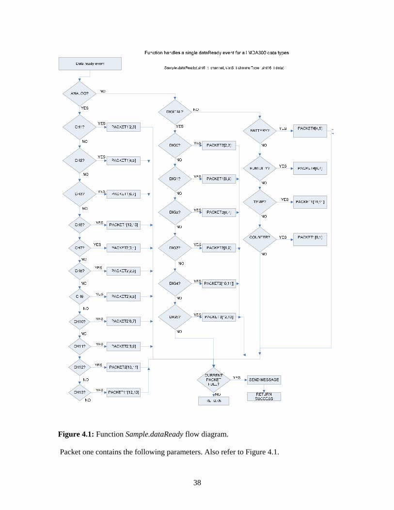
case 5: packet[3].data[12]=data & 0xff; //least sign bts packet[3].data[13]=(data >> 8) & 0xff; atomic {msg_status[3]|=0x20;} //flags when packet break; //is full } Refer to Figure 4.1, which represents the complete MDA300 data types flow diagram.
The flow diagram also corresponds to the code in the included CD, refer to Appendix F
for more information and Appendix I for included CD read me file.

37
4.3.3 mda300.c
This file handles conversion to engineering units of mda300 packets, and it’s located at:
c:/tinyos/cygwin/opt/tinyos-1.x/contrib/xbow/tools/src/xlisten/boards
There are five different packets send by the mote + MDA board. These packets are
packed by the nesC component and module running in the mote called
XSensorMDA300M.nc. Specific outputs provide five different conversion functions
within the mda300.c file. The content of each packet is determined by the nesC Module
XSensorMDA300M.nc as mentioned before in Section 4.3.1. There are six sensor
parameters that need to be formatted/converted and in the module those sensor reading
were specified to compose packet #1.
38
Figure 4.1: Function Sample.dataReady flow diagram. Packet one contains the following parameters. Also refer to Figure 4.1.
39
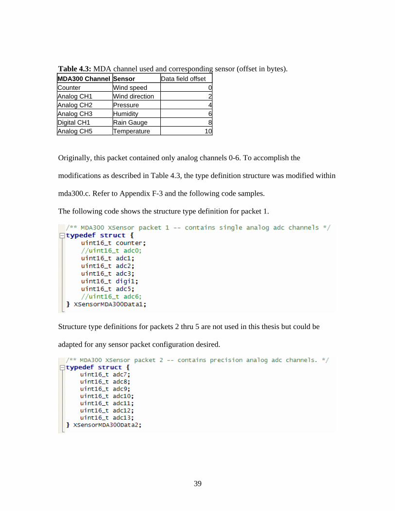
Table 4.3: MDA channel used and corresponding sensor (offset in bytes). MDA300 Channel Sensor Data field offset Counter Wind speed 0Analog CH1 Wind direction 2Analog CH2 Pressure 4Analog CH3 Humidity 6Digital CH1 Rain Gauge 8Analog CH5 Temperature 10 Originally, this packet contained only analog channels 0-6. To accomplish the
modifications as described in Table 4.3, the type definition structure was modified within
mda300.c. Refer to Appendix F-3 and the following code samples.
The following code shows the structure type definition for packet 1.
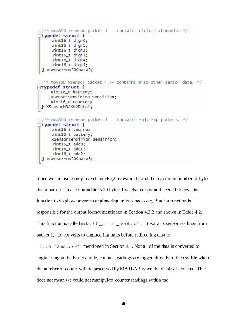
Structure type definitions for packets 2 thru 5 are not used in this thesis but could be
adapted for any sensor packet configuration desired.
40
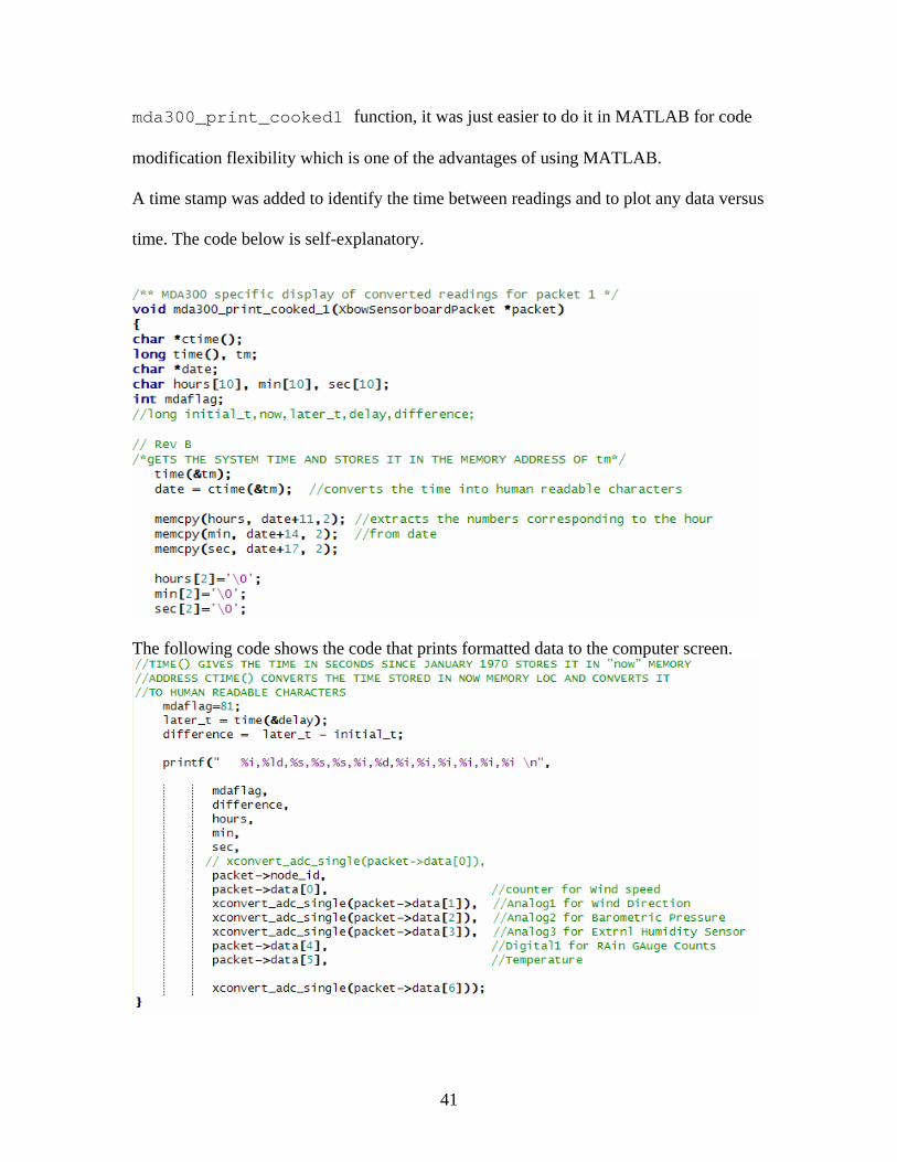
Since we are using only five channels (2 bytes/field), and the maximum number of bytes
that a packet can accommodate is 29 bytes, five channels would need 10 bytes. One
function to display/convert to engineering units is necessary. Such a function is
responsible for the output format mentioned in Section 4.2.2 and shown in Table 4.2.
This function is called mda300_print_cooked1. It extracts sensor readings from
packet 1, and converts to engineering units before redirecting data to
‘file_name.csv’ mentioned in Section 4.1. Not all of the data is converted to
engineering units. For example, counter readings are logged directly to the csv file where
the number of counts will be processed by MATLAB when the display is created. That
does not mean we could not manipulate counter readings within the
41
mda300_print_cooked1 function, it was just easier to do it in MATLAB for code
modification flexibility which is one of the advantages of using MATLAB.
A time stamp was added to identify the time between readings and to plot any data versus
time. The code below is self-explanatory.
The following code shows the code that prints formatted data to the computer screen.
42
This function prints a hard-coded flag to identify data coming from an mda300 board.
The base station receives data from any board in its surroundings. Since we will be
running a GPS board at the same time as the mda300CA, a distinct flag will be used for
each board. In this case mdaflag=81 specified data coming from MDA300CA board.
The next line variable called “difference” holds the time difference in seconds
from when the mda board was turned on and the next packet transmitted. The variables
“hours” ”min” and “sec” are self-explanatory. The next lines of code display
node ID remember the user can specify a different node id and the base station should
have a node id = 0. The next lines access the TOS_MSG data field offsetting each time
for a different sensor reading. Notice that for analog 1,2,3 the data becomes an argument
of the function xconvert_adc_single().
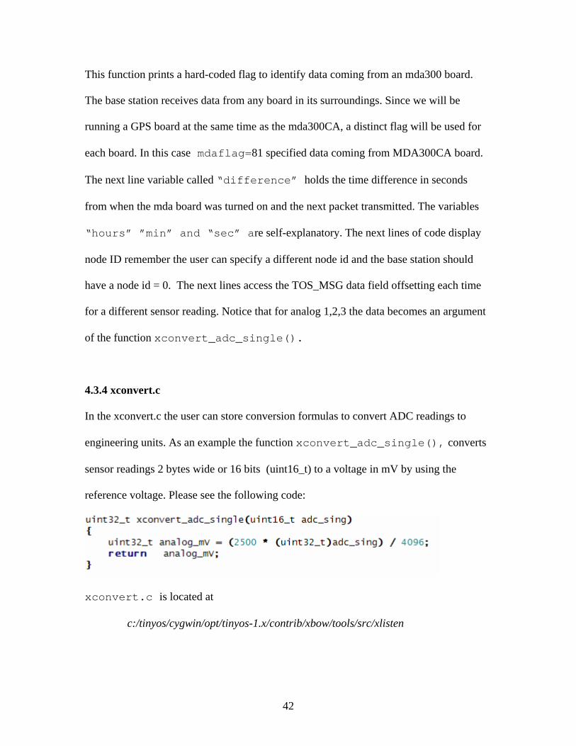
4.3.4 xconvert.c
In the xconvert.c the user can store conversion formulas to convert ADC readings to
engineering units. As an example the function xconvert_adc_single(), converts
sensor readings 2 bytes wide or 16 bits (uint16_t) to a voltage in mV by using the
reference voltage. Please see the following code:
xconvert.c is located at
c:/tinyos/cygwin/opt/tinyos-1.x/contrib/xbow/tools/src/xlisten

43
Chapter 5 System Integration In this chapter the discussion will turn to the specific sensors used and how the
conversion formulas were found or calculated. These formulas are used for converting
sensor voltage output readings to engineering units, which will be used by MATLAB to
create plots of sensor readings vs. time.
5.1 Relative Humidity Sensor
A relative humidity sensor’s output voltage relates directly to relative humidity from 0%
to 100%. Humirel ‘HM1500’ was used for this project.
Figure 5.1: Humirel model HM1500.
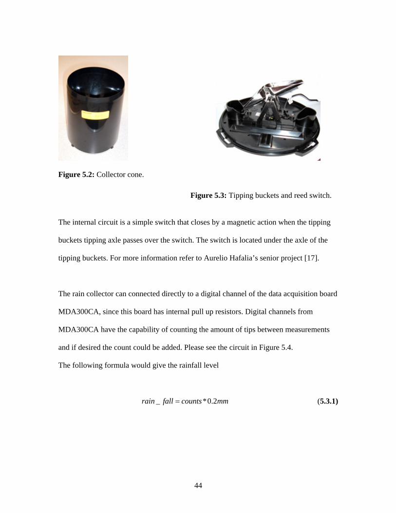
Please read reference senior project [34] for more information. 5.2 Rain Gauge
A Rain gauge counts the amount of waterfall in a certain location. It consists of a
collector cone, and two tipping buckets. Rain enters the collector cone, and collects in
one chamber of the tipping bucket. The bucket tips when it has collected an amount of
water equal to the increment in which the collector measures (0.01" or 0.2 mm) [30]. As
the bucket tips, it causes a switch closure and brings the second tipping bucket chamber
into position. The rain water drains out through the screened drains in the base of the
collector.
44
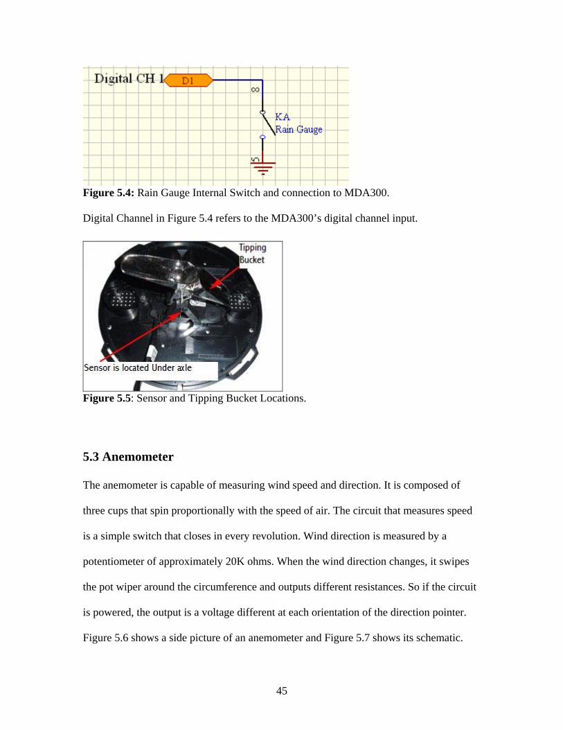
Figure 5.2: Collector cone. Figure 5.3: Tipping buckets and reed switch.
The internal circuit is a simple switch that closes by a magnetic action when the tipping
buckets tipping axle passes over the switch. The switch is located under the axle of the
tipping buckets. For more information refer to Aurelio Hafalia’s senior project [17].
The rain collector can connected directly to a digital channel of the data acquisition board
MDA300CA, since this board has internal pull up resistors. Digital channels from
MDA300CA have the capability of counting the amount of tips between measurements
and if desired the count could be added. Please see the circuit in Figure 5.4.
The following formula would give the rainfall level
_ *0.2rain fall counts mm= (5.3.1)
45
Figure 5.4: Rain Gauge Internal Switch and connection to MDA300. Digital Channel in Figure 5.4 refers to the MDA300’s digital channel input.
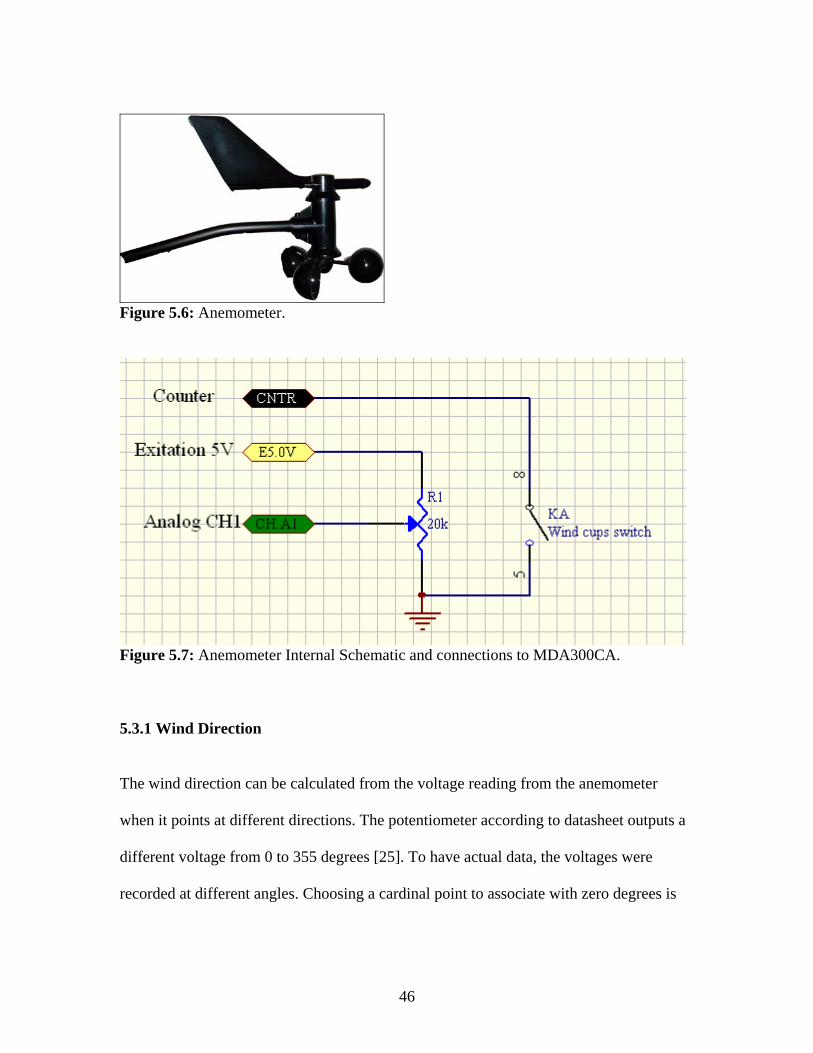
Figure 5.5: Sensor and Tipping Bucket Locations. 5.3 Anemometer
The anemometer is capable of measuring wind speed and direction. It is composed of
three cups that spin proportionally with the speed of air. The circuit that measures speed
is a simple switch that closes in every revolution. Wind direction is measured by a
potentiometer of approximately 20K ohms. When the wind direction changes, it swipes
the pot wiper around the circumference and outputs different resistances. So if the circuit
is powered, the output is a voltage different at each orientation of the direction pointer.
Figure 5.6 shows a side picture of an anemometer and Figure 5.7 shows its schematic.
46
Figure 5.6: Anemometer.
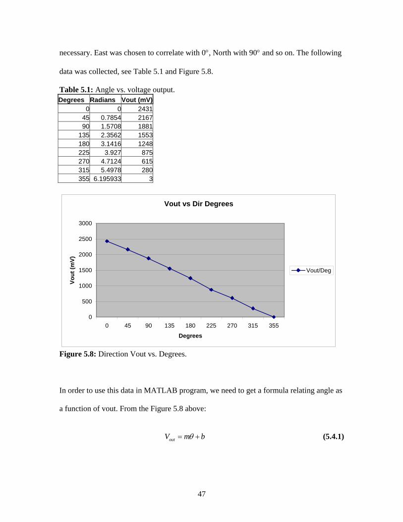
Figure 5.7: Anemometer Internal Schematic and connections to MDA300CA. 5.3.1 Wind Direction The wind direction can be calculated from the voltage reading from the anemometer
when it points at different directions. The potentiometer according to datasheet outputs a
different voltage from 0 to 355 degrees [25]. To have actual data, the voltages were
recorded at different angles. Choosing a cardinal point to associate with zero degrees is
47
necessary. East was chosen to correlate with 0°, North with 90° and so on. The following
data was collected, see Table 5.1 and Figure 5.8.
Table 5.1: Angle vs. voltage output. Degrees Radians Vout (mV)
0 0 243145 0.7854 216790 1.5708 1881
135 2.3562 1553180 3.1416 1248225 3.927 875270 4.7124 615315 5.4978 280355 6.195933 3
Vout vs Dir Degrees
0
500
1000
1500
2000
2500
3000
0 45 90 135 180 225 270 315 355
Degrees
Vout
(mV)
Vout/Deg
Figure 5.8: Direction Vout vs. Degrees.
In order to use this data in MATLAB program, we need to get a formula relating angle as
a function of vout. From the Figure 5.8 above:
outV m bθ= + (5.4.1)
48
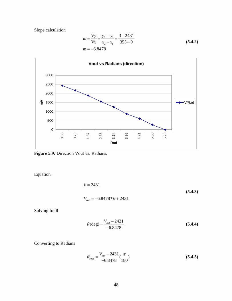
Slope calculation 2 1
2 1
3 2431355 0
6.8478
y yymx x x
m
− −= = =
− −= −
VV (5.4.2)
Vout vs Radians (direction)
0
500
1000
1500
2000
2500
3000
0.00
0.79
1.57
2.36
3.14
3.93
4.71
5.50
6.20
Rad
mV V/Rad
Figure 5.9: Direction Vout vs. Radians. Equation
2431
6.8478* 2431out
b
V θ
=
= − + (5.4.3)
Solving for θ
2431(deg)6.8478
outVθ −=
− (5.4.4)
Converting to Radians
2431( )6.8478 180
outrads
V πθ −=
− (5.4.5)
49
Formula 5.4.5 will be used to plot the wind direction in a polar plot showing an actual
arrow showing the wind direction.
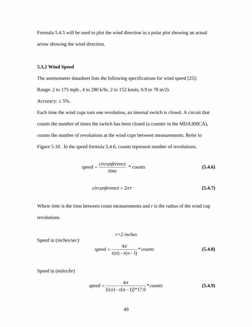
5.3.2 Wind Speed
The anemometer datasheet lists the following specifications for wind speed [25]:
Range: 2 to 175 mph., 4 to 280 k/hr, 2 to 152 knots, 0.9 to 78 m/2s
Accuracy: ± 5%.
Each time the wind cups turn one revolution, an internal switch is closed. A circuit that
counts the number of times the switch has been closed (a counter in the MDA300CA),
counts the number of revolutions at the wind cups between measurements. Refer to
Figure 5.10. In the speed formula 5.4.6, counts represent number of revolutions.
circunferencespeed
time= * counts (5.4.6)
2circunference rπ= (5.4.7)
Where time is the time between count measurements and r is the radius of the wind cup
revolutions.
r=2 inches
Speed in (inches/sec) 4 *
( ) ( 1)speed counts
t n t nπ
=− −
(5.4.8)
Speed in (miles/hr)
4 *[ ( ) ( 1)]*17.6
speed countst n t n
π=
− − (5.4.9)
50
Time between measurements is calculated by subtracting the current measurement time
t(n) minus the time at which the last measurement was taken t(n-1). Table 5.2 is an
example of the data redirected to a *.csv file
Table 5.2: Sample data from sensors.csv file obtained by Xlisten and MDA300CA. board id elapsed time hr Min sec mote id Counts vout (direction)
81 0 13 52 2 88 0 120281 9 13 52 11 88 3 120381 18 13 52 20 88 5 120181 27 13 52 29 88 1 1204
We are interested in elapsed time (time) and counts columns; See Table 5.3. Table 5.3: Columns used in this example.
n elapsed time Counts
vout (direction)
1 0 0 1202 2 9 3 1203 3 18 5 1201 4 27 1 1204
Calculation of speed at n=3, by using formula (5.4.8).
t(n)=t(3)=18
t(n-1)=9
t(n)-t(n-1)=18-9=9 secs
counts= # of revolutions=5
The speed in mi/hr is
4 *5 0.397[18 9]*17.6
speed π= =
−(Mi/hr)
Please look at the MATLAB code in Appendix H for the code application of above
equations and calculations.
51
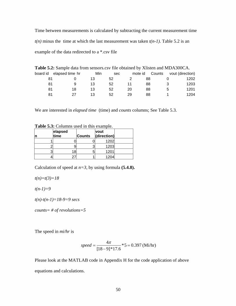
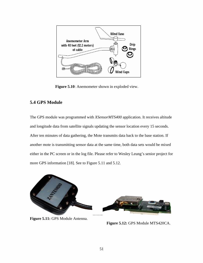
Figure 5.10: Anemometer shown in exploded view. 5.4 GPS Module
The GPS module was programmed with XSensorMTS400 application. It receives altitude and longitude data from satellite signals updating the sensor location every 15 seconds. After ten minutes of data gathering, the Mote transmits data back to the base station. If another mote is transmitting sensor data at the same time, both data sets would be mixed either in the PC screen or in the log file. Please refer to Wesley Leung’s senior project for more GPS information [18]. See to Figure 5.11 and 5.12.
…….. Figure 5.11: GPS Module Antenna. Figure 5.12: GPS Module MTS420CA.

52
5.5 Graphical User Interface (GUI) Development
The Graphical user interface, or GUI, was created after all of the sensors were
characterized, and all the formulas were gathered. In this Section we will discuss how
requirements from Section 2.3 can be met by the GUI application. The GUI was to be
created in MATLAB, which includes a Graphical User Interface Development
Environment called GUIDE.
First, the layout of the GUI was created having in mind the required six plots of
data needed to be graphed. In the GUI, there are four plots displayed at all times. Two
popup lists choose the two plots on the right of the display; the popup lists lets the user
chose what data is to be plotted in each plot. Refer to Figure 5.13 to see the final GUI
layout and the popup lists.
Once the layout was done, the m file was coded. The m file is the file extension
for the Program file associated with MATLAB. Each of the GUI components can be
controlled thru the m file code as well as each component has a function that is called
each time the component is activated. For example, each time a button is pressed, its
function is called and the code within it is executed. For more detail about the GUI
development environment please read reference [15]; also read Appendix E for flow
diagrams and m-file code.
There are three components that control how the GUI behaves:
• Update plots pushbutton
• GPS Pressure popup menu
• Humidity Temperature popup menu
53
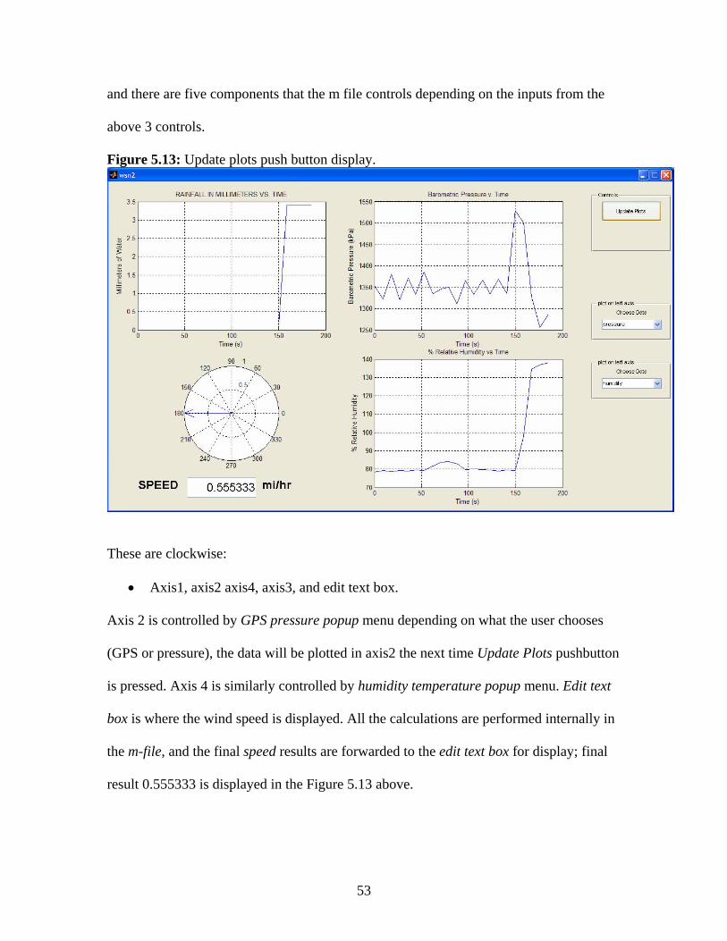
and there are five components that the m file controls depending on the inputs from the
above 3 controls.
Figure 5.13: Update plots push button display.
These are clockwise:
• Axis1, axis2 axis4, axis3, and edit text box.
Axis 2 is controlled by GPS pressure popup menu depending on what the user chooses
(GPS or pressure), the data will be plotted in axis2 the next time Update Plots pushbutton
is pressed. Axis 4 is similarly controlled by humidity temperature popup menu. Edit text
box is where the wind speed is displayed. All the calculations are performed internally in
the m-file, and the final speed results are forwarded to the edit text box for display; final
result 0.555333 is displayed in the Figure 5.13 above.
54
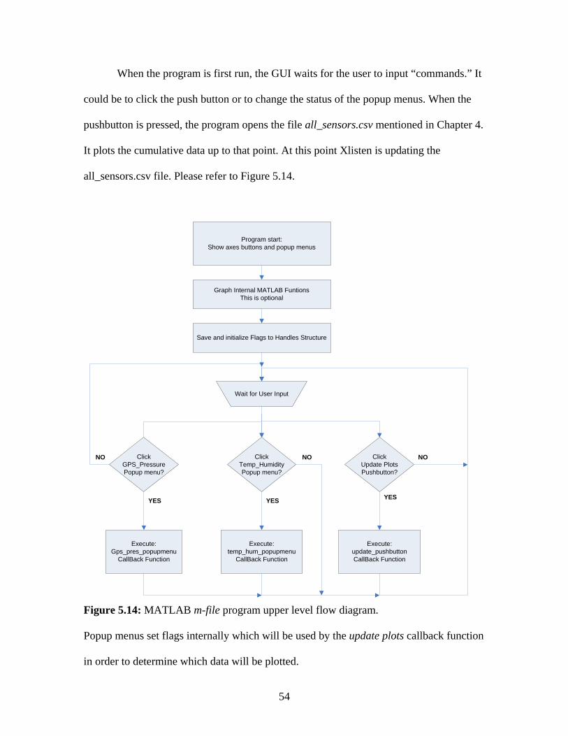
When the program is first run, the GUI waits for the user to input “commands.” It
could be to click the push button or to change the status of the popup menus. When the
pushbutton is pressed, the program opens the file all_sensors.csv mentioned in Chapter 4.
It plots the cumulative data up to that point. At this point Xlisten is updating the
all_sensors.csv file. Please refer to Figure 5.14.
Program start:Show axes buttons and popup menus
Graph Internal MATLAB FuntionsThis is optional
Save and initialize Flags to Handles Structure
Wait for User Input
ClickGPS_PressurePopup menu?
ClickTemp_HumidityPopup menu?
ClickUpdate Plots Pushbutton?
Execute:Gps_pres_popupmenu
CallBack Function
Execute:temp_hum_popupmenu
CallBack Function
Execute:update_pushbuttonCallBack Function
YES YES YES
NO NO NO
Figure 5.14: MATLAB m-file program upper level flow diagram. Popup menus set flags internally which will be used by the update plots callback function
in order to determine which data will be plotted.
55
When the user presses the update plots pushbutton, the program control goes to update
plots callback function and performs all the commands listed inside that function.
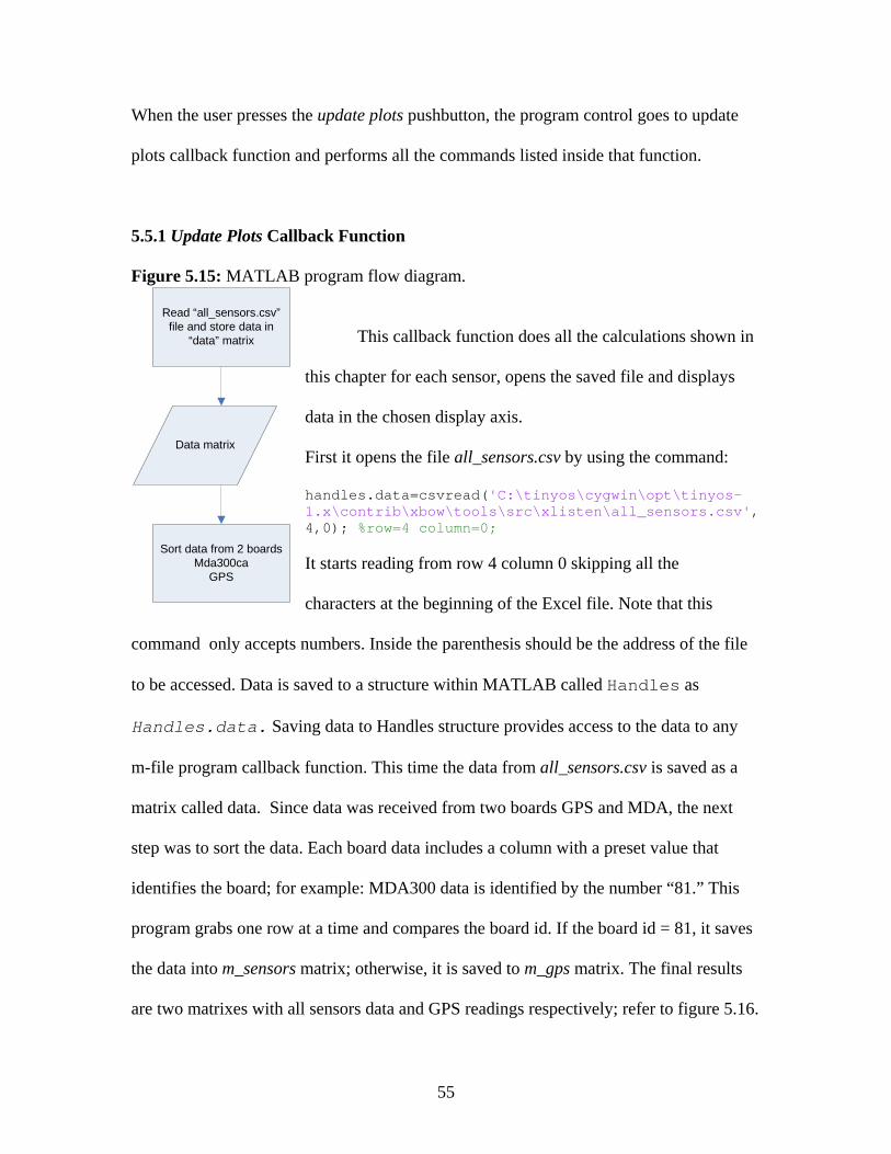
5.5.1 Update Plots Callback Function Figure 5.15: MATLAB program flow diagram.
This callback function does all the calculations shown in
this chapter for each sensor, opens the saved file and displays
data in the chosen display axis.
First it opens the file all_sensors.csv by using the command:
handles.data=csvread('C:\tinyos\cygwin\opt\tinyos-1.x\contrib\xbow\tools\src\xlisten\all_sensors.csv',4,0); %row=4 column=0; It starts reading from row 4 column 0 skipping all the
characters at the beginning of the Excel file. Note that this
command only accepts numbers. Inside the parenthesis should be the address of the file
to be accessed. Data is saved to a structure within MATLAB called Handles as
Handles.data. Saving data to Handles structure provides access to the data to any
m-file program callback function. This time the data from all_sensors.csv is saved as a
matrix called data. Since data was received from two boards GPS and MDA, the next
step was to sort the data. Each board data includes a column with a preset value that
identifies the board; for example: MDA300 data is identified by the number “81.” This
program grabs one row at a time and compares the board id. If the board id = 81, it saves
the data into m_sensors matrix; otherwise, it is saved to m_gps matrix. The final results
are two matrixes with all sensors data and GPS readings respectively; refer to figure 5.16.
Read “all_sensors.csv” file and store data in
“data” matrix
Data matrix
Sort data from 2 boardsMda300ca
GPS
56
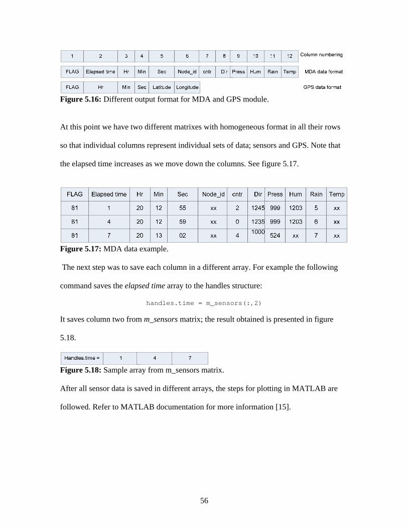
Figure 5.16: Different output format for MDA and GPS module.
At this point we have two different matrixes with homogeneous format in all their rows
so that individual columns represent individual sets of data; sensors and GPS. Note that
the elapsed time increases as we move down the columns. See figure 5.17.
Figure 5.17: MDA data example. The next step was to save each column in a different array. For example the following
command saves the elapsed time array to the handles structure:
handles.time = m_sensors(:,2)
It saves column two from m_sensors matrix; the result obtained is presented in figure
5.18.
Figure 5.18: Sample array from m_sensors matrix.
After all sensor data is saved in different arrays, the steps for plotting in MATLAB are
followed. Refer to MATLAB documentation for more information [15].
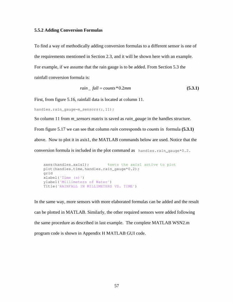
57
5.5.2 Adding Conversion Formulas
To find a way of methodically adding conversion formulas to a different sensor is one of
the requirements mentioned in Section 2.3, and it will be shown here with an example.
For example, if we assume that the rain gauge is to be added. From Section 5.3 the
rainfall conversion formula is:
_ *0.2rain fall counts mm= (5.3.1)
First, from figure 5.16, rainfall data is located at column 11.
handles.rain_gauge=m_sensors(:,11);
So column 11 from m_sensors matrix is saved as rain_gauge in the handles structure.
From figure 5.17 we can see that column rain corresponds to counts in formula (5.3.1)
above. Now to plot it in axis1, the MATLAB commands below are used. Notice that the
conversion formula is included in the plot command as handles.rain_gauge*0.2.
axes(handles.axis1); %sets the axis1 active to plot plot(handles.time,handles.rain_gauge*0.2); grid xlabel('Time (s)') ylabel('Millimeters of Water') Title('RAINFALL IN MILLIMETERS VS. TIME')
In the same way, more sensors with more elaborated formulas can be added and the result
can be plotted in MATLAB. Similarly, the other required sensors were added following
the same procedure as described in last example. The complete MATLAB WSN2.m
program code is shown in Appendix H MATLAB GUI code.
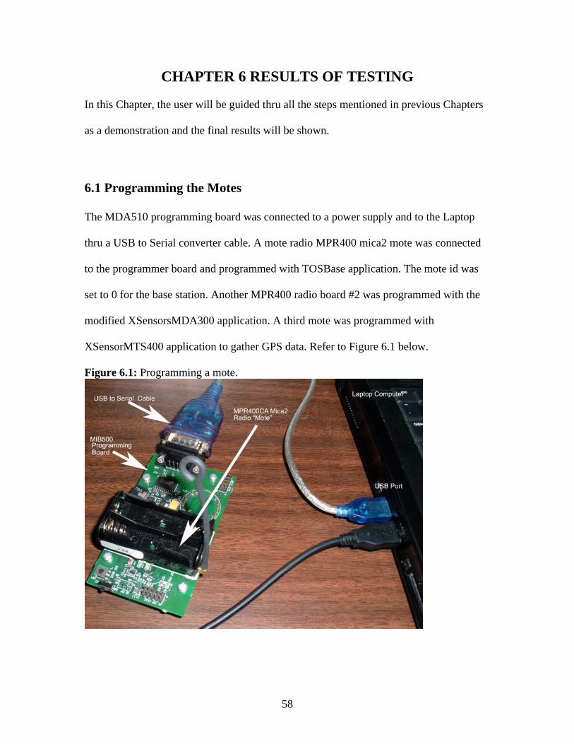
58
CHAPTER 6 RESULTS OF TESTING In this Chapter, the user will be guided thru all the steps mentioned in previous Chapters
as a demonstration and the final results will be shown.
6.1 Programming the Motes
The MDA510 programming board was connected to a power supply and to the Laptop
thru a USB to Serial converter cable. A mote radio MPR400 mica2 mote was connected
to the programmer board and programmed with TOSBase application. The mote id was
set to 0 for the base station. Another MPR400 radio board #2 was programmed with the
modified XSensorsMDA300 application. A third mote was programmed with
XSensorMTS400 application to gather GPS data. Refer to Figure 6.1 below.
Figure 6.1: Programming a mote.
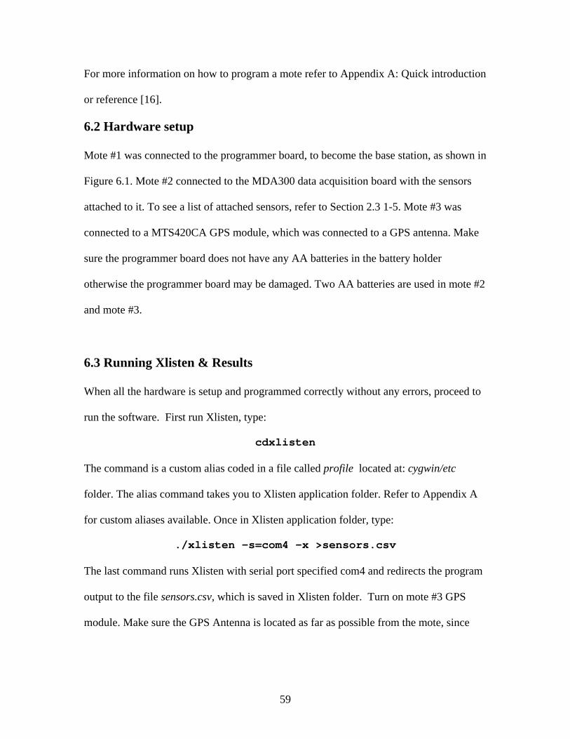
59
For more information on how to program a mote refer to Appendix A: Quick introduction
or reference [16].
6.2 Hardware setup
Mote #1 was connected to the programmer board, to become the base station, as shown in
Figure 6.1. Mote #2 connected to the MDA300 data acquisition board with the sensors
attached to it. To see a list of attached sensors, refer to Section 2.3 1-5. Mote #3 was
connected to a MTS420CA GPS module, which was connected to a GPS antenna. Make
sure the programmer board does not have any AA batteries in the battery holder
otherwise the programmer board may be damaged. Two AA batteries are used in mote #2
and mote #3.
6.3 Running Xlisten & Results
When all the hardware is setup and programmed correctly without any errors, proceed to
run the software. First run Xlisten, type:
cdxlisten
The command is a custom alias coded in a file called profile located at: cygwin/etc
folder. The alias command takes you to Xlisten application folder. Refer to Appendix A
for custom aliases available. Once in Xlisten application folder, type:
./xlisten –s=com4 –x >sensors.csv
The last command runs Xlisten with serial port specified com4 and redirects the program
output to the file sensors.csv, which is saved in Xlisten folder. Turn on mote #3 GPS
module. Make sure the GPS Antenna is located as far as possible from the mote, since
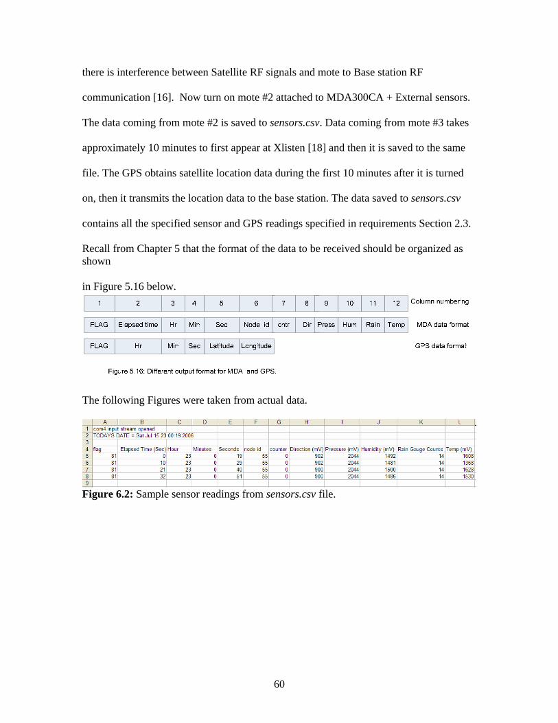
60
there is interference between Satellite RF signals and mote to Base station RF
communication [16]. Now turn on mote #2 attached to MDA300CA + External sensors.
The data coming from mote #2 is saved to sensors.csv. Data coming from mote #3 takes
approximately 10 minutes to first appear at Xlisten [18] and then it is saved to the same
file. The GPS obtains satellite location data during the first 10 minutes after it is turned
on, then it transmits the location data to the base station. The data saved to sensors.csv
contains all the specified sensor and GPS readings specified in requirements Section 2.3.
Recall from Chapter 5 that the format of the data to be received should be organized as shown in Figure 5.16 below.
The following Figures were taken from actual data.
Figure 6.2: Sample sensor readings from sensors.csv file.
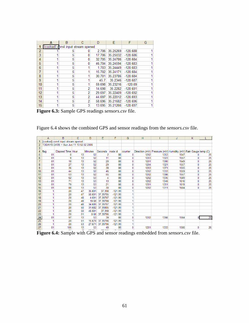
61
Figure 6.3: Sample GPS readings sensors.csv file.
Figure 6.4 shows the combined GPS and sensor readings from the sensors.csv file.
Figure 6.4: Sample with GPS and sensor readings embedded from sensors.csv file.

62
6.4 Running MATLAB & Results
MATLAB can be run just after Xlisten. Open WSN2.fig and run it. WSN2.fig is the
name given to the GUI created for this project. With the creation of the GUI, the
following requirements were met (from Section 2.3)
It integrates the following sensor data:
1. Wind direction
2. Wind speed
3. Relative Humidity
4. Pressure
5. Rain Gauge
6. Temperature
7. GPS sensor
8. The GUI can show four data plots at a time:
1. Rain gauge readings vs. time
2. Either GPS location (Latitude, Longitude) or Pressure (mBar)
3. Wind direction and speed in one plot
4. Either Relative humidity (%) or temperature
For example if a file similar to Figure 6.4 with readings from GPS and MDA boards, a
plot like the one on Figure 6.5 is obtained. Figure 6.6 shows rain gauge readings.
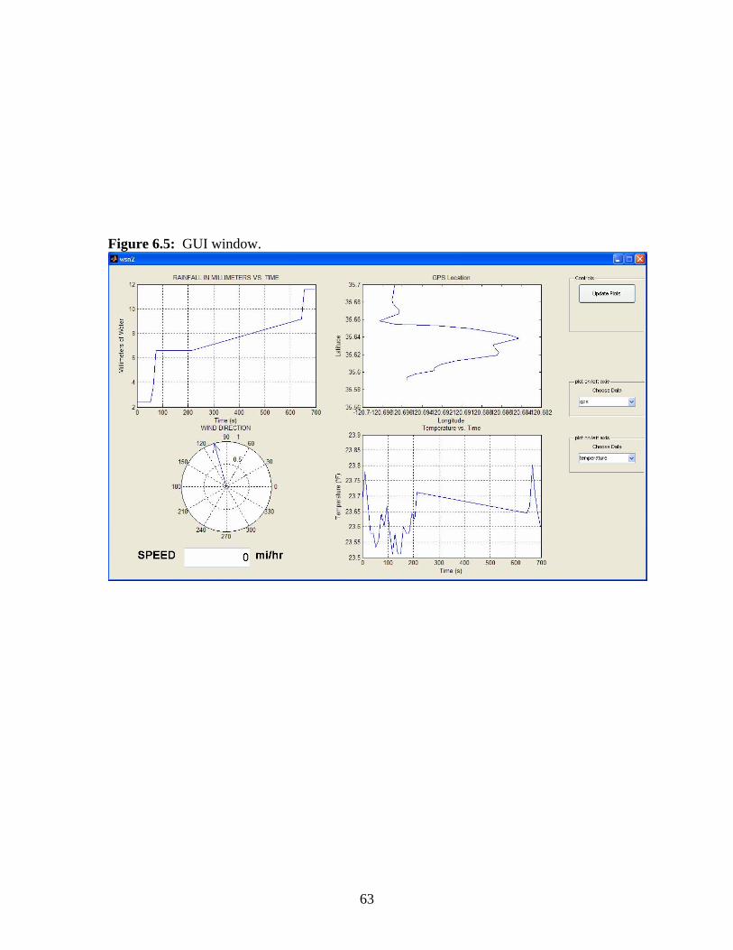
63
Figure 6.5: GUI window.
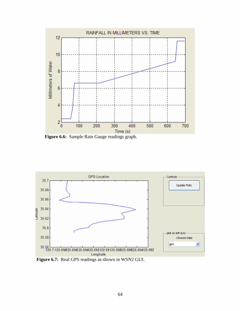
64
Figure 6.6: Sample Rain Gauge readings graph.
Figure 6.7: Real GPS readings as shown in WSN2 GUI.
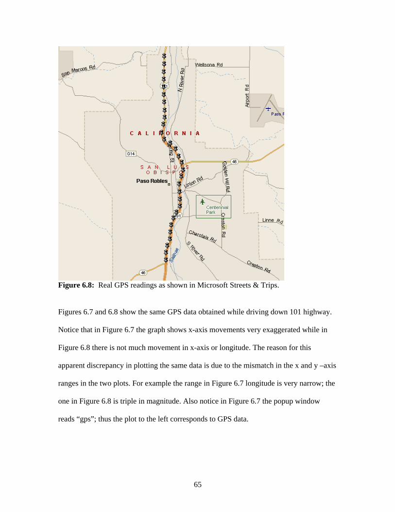
65
Figure 6.8: Real GPS readings as shown in Microsoft Streets & Trips. Figures 6.7 and 6.8 show the same GPS data obtained while driving down 101 highway.
Notice that in Figure 6.7 the graph shows x-axis movements very exaggerated while in
Figure 6.8 there is not much movement in x-axis or longitude. The reason for this
apparent discrepancy in plotting the same data is due to the mismatch in the x and y –axis
ranges in the two plots. For example the range in Figure 6.7 longitude is very narrow; the
one in Figure 6.8 is triple in magnitude. Also notice in Figure 6.7 the popup window
reads “gps”; thus the plot to the left corresponds to GPS data.
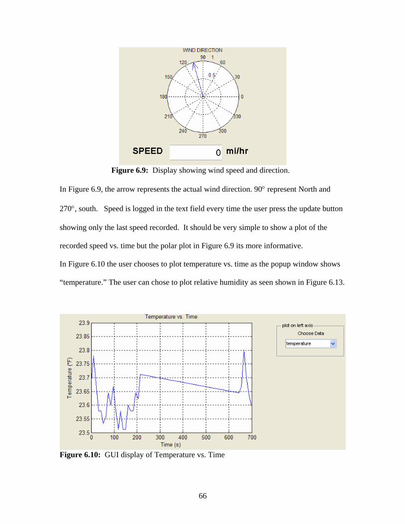
66
Figure 6.9: Display showing wind speed and direction. In Figure 6.9, the arrow represents the actual wind direction. 90° represent North and
270°, south. Speed is logged in the text field every time the user press the update button
showing only the last speed recorded. It should be very simple to show a plot of the
recorded speed vs. time but the polar plot in Figure 6.9 its more informative.
In Figure 6.10 the user chooses to plot temperature vs. time as the popup window shows
“temperature.” The user can chose to plot relative humidity as seen shown in Figure 6.13.
Figure 6.10: GUI display of Temperature vs. Time
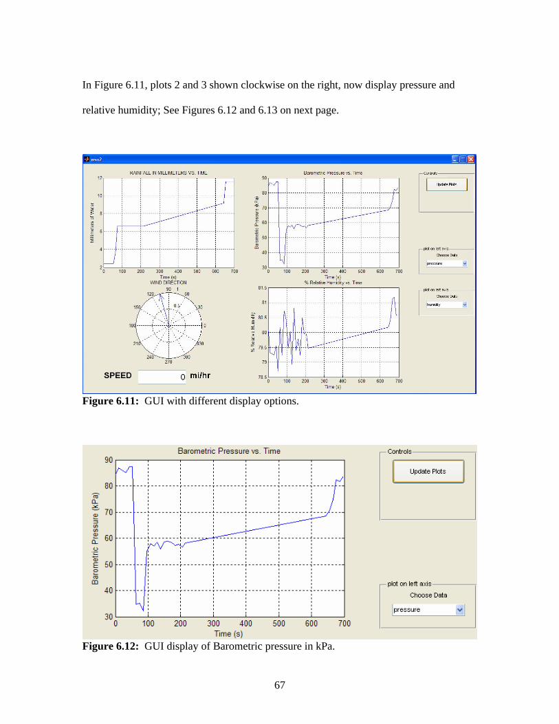
67
In Figure 6.11, plots 2 and 3 shown clockwise on the right, now display pressure and
relative humidity; See Figures 6.12 and 6.13 on next page.
Figure 6.11: GUI with different display options.
Figure 6.12: GUI display of Barometric pressure in kPa.
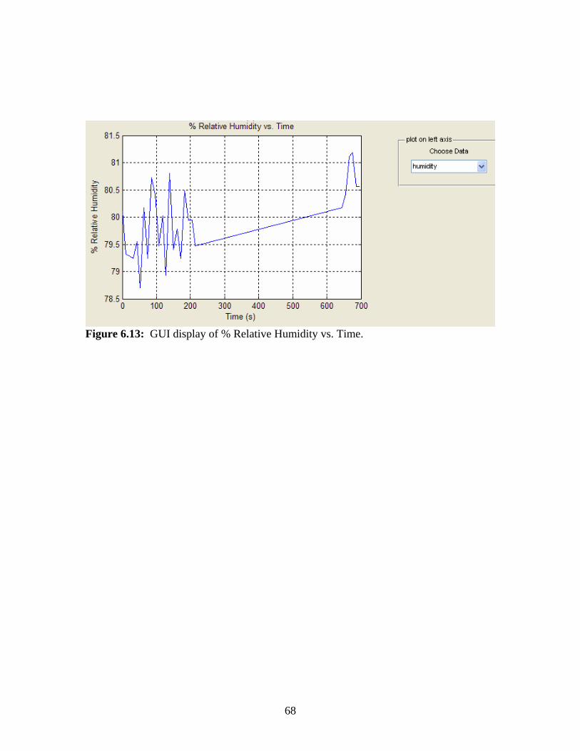
68
Figure 6.13: GUI display of % Relative Humidity vs. Time.
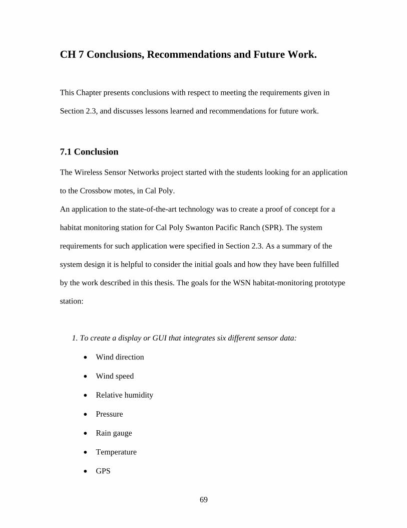
69
CH 7 Conclusions, Recommendations and Future Work.
This Chapter presents conclusions with respect to meeting the requirements given in
Section 2.3, and discusses lessons learned and recommendations for future work.
7.1 Conclusion
The Wireless Sensor Networks project started with the students looking for an application
to the Crossbow motes, in Cal Poly.
An application to the state-of-the-art technology was to create a proof of concept for a
habitat monitoring station for Cal Poly Swanton Pacific Ranch (SPR). The system
requirements for such application were specified in Section 2.3. As a summary of the
system design it is helpful to consider the initial goals and how they have been fulfilled
by the work described in this thesis. The goals for the WSN habitat-monitoring prototype
station:
1. To create a display or GUI that integrates six different sensor data:
• Wind direction
• Wind speed
• Relative humidity
• Pressure
• Rain gauge
• Temperature
• GPS

70
To address all the above requirements the following was achieved:
First, an overview of each sensor is presented. Since each undergraduate student
researched individual sensors, only the sensors that needed more information
from the senior project papers are explained in Sections 5.1 to 5.4. The
conversion formulas and output units were defined.
2. A base station computer should gather sensor data.
Xlisten was modified to achieve this goal. In Sections 4.2 Xlisten is presented and
in Appendix B the Xlisten manual is reproduced for convenience.
3. To develop a methodical way of changing/adding new sensors to the system
Information is presented in Sections 4.2.1, 4.2.2, 4.3 on how to modify the
software and an example sensor is given in Section 4.3.2.
4. To develop a way of adding or modifying the sensor engineering conversion Formulas. Modifying engineering formulas is easily accomplished by adding the formula to
a custom MATLAB code (WSN2.m). It is described in Section 5.5 specifically in
Section 5.5.2. A MATLAB m-file program flow diagram is presented in
Appendix E.
5. To develop one GUI display with four plot windows; plot a, b, c and d labeled clockwise for reference
• Rain gauge readings vs. time
• GPS (Latitude Longitude) or Pressure (mBar)
• Wind speed and direction in one plot

71
• Relative Humidity (%hum) or Temperature (F)
The GUI display is described in Chapter 5 and code for the GUI is presented in
Appendix H. Final results and sample data graphs are shown in Chapter 6.
All the requirements were met. Even though the display is simple, it gives a perspective
on what can be done when the technology matures and more development is done to
TinyOS and the mote hardware. One of the major obstacles to the progress of the project
was the understanding of tinyOS programming approach. In the beginning it was
intended to use ad-hoc networking but it proved to be very challenging and somewhat a
daunting task, since some of the features advertised as working, actually have bugs or
simply don’t work [16]. When high-level programming languages become available to
program motes the task will be simpler and the range of applications will be broader.
The GPS display shows position latitude and longitude accurately within few feet but it
does not show a map to reference the location. It shows relative position and movement
from a starting point. When the data is used with Microsoft Streets and Maps, the data
acquired proves to be relatively simple and useful. Refer to figure 6.8.
In future releases of TinyOS the approach shown in this paper could be used. MATLAB
code can be used with minor or no modifications. That does not apply to Xlisten code.
The release of tinyOS 2.0 will be different since it is a new OS from the ground up [1].
Xlisten code shown here most probably is not going to work with tinyOS 2.0, but
certainly the new operating system should provide a similar approach.

72
The approach shown in this paper is limited by various factors. Its limited by the
maximum number of data rows a csv file can accommodate. Such number is 65536 for
Microsoft Excel 2000 (9.0.2720). Speed is not critical In the application presented here.
It could be critical if the application requires fast transmission of data; for example if the
application is a control system where the feedback needs to be transmitted fast back to
the controlling algorithm, the control system could fail due to the lack of data
transmission speed. The maximum distance from mote to mote is another limitation. As
the mote separation distance increases, the signal strength decreases causing dropped
packets and a decrease in overall system efficiency. Memory of the mote is not a
limitation in this application. Memory could be a limitation if the data were to be stored
and processed at the mote. The mote has 128kB of program memory so the application
would be limited if the program required were to exceed such limit.
The flexibility of this project it is its most important feature. It was shown that
sensors and their respective code could be added or removed in a systematic way. More
data acquisition boards can be added and identified by programming the board id or flag
to the file mda300.c. The GUI display has some flexibility; it has options to plot the data
that the user chooses. The number of motes is limited by the number of node id and the
group id that can be added. Up to 256 groups with 65534 nodes each can co-exist with
one base station [16].
This work was an initial study of Wireless Sensor Networks which at the moment
was a break into new ground intended as a proof of concept for a Swanton Pacific Ranch
possible application. In this project, ad-hoc networking is not applied. It assumes that the
network is already established and programmed. Implementing Ad-hoc networking

73
would not affect the way Xlisten receives data packets; the data is always forwarded to
the base station, and Xlisten always receives data from the base station, so the approach
to display data in this paper would still apply.
7.2 Recommendations and lessons learned
The following are some of the recommendations learned by experience. They proved to
be useful in special circumstances.
• Use aliases to navigate between folders as shown in Appendix A. It makes it
easier to navigate thru tinyOS directories.
• If more projects are to be developed with tinyOS, a dedicated group of
students should be assigned to learn tinyOS programming. They should be
majoring in CPE or CS.
• To improve on this thesis or to get started in tinyOS, I suggest to read the
TinyOS tutorials [1] along with the lab development thesis paper [16], all
four senior projects related to this work [17,18,34,35], then read this paper.
• When reviewing the thesis work in reference [16] on page 3 of lab 1 of
student version Customizing CygWin for TinyOS Programming, after
modifying the specified custom files A-1, A-2, A-3, A-4, the application did
not do what was expected. To fix it, all the commands were manually typed
in a cygwin session and then the application could be run. The problem was
unknown since only a different PC was used, and the setup was the same.
• After installing MATLAB version 7.2.0.232 (R2006a) , Xlisten could not
run. It flagged an error saying cygwin1.dll was missing. Supposedly the
74
most current version of cygwin1.dll was not in the correct folder
(C:\tinyos\cigwin\bin). After a search for that file in the C: drive, I found
another version of cygwin1.dll located in the MATLAB directory; the new
file was renamed and after that, Xlisten functioned as usual.
7.3 Future Work
There are several improvements that can be done to this project; for example:
• To integrate ad-hoc routing to this demonstration.
• With the new release of TinyOS 2.0 start by applying the same approach used in
this project and then implement it.
• Develop a program similar to Xlisten that ‘listens’ to the serial port and make it
customizable so any type of packet format can be deciphered and read.
• Make a website where the user can chose what data to graph. To do this, a
database can be added so there is access to past sensor data available to compare
with live data and then plot them in a single graph.
• Chose what parameters to plot or to measure by the motes; reprogram the motes
using IN-Network programming.
• Reprogram the motes thru a website
• The GPS display can be improved by adding a database with maps. Add features
to calculate speed by using relative target locations at measured time intervals.
For example, the GPS described in this project samples approximately each 15
seconds. Taking into account the earth curvature and direction of travel, the speed
can be calculated.

75
• Apply WSN to a greenhouse environment as mentioned in Appendix C.
• Finally, future projects that add functionality to projects similar to this one would
take advantage of the work already done and that has been developed. Continue to
explore the habitat monitoring applications to WSN and at the same time to
provide research opportunities for thesis or senior project work. This should be
the end result of the ideas that have been presented in this thesis.
76
REFERENCES: [1] TinyOS. University of California Berkeley (July 2, 2005); accessed 2 July 2006;
available at http://www.tinyos.net [2] Crossbow Technology; accessed 27 May 2005, available from
http://www.xbow.com/ [3] “MOTE-VIEW 1.0 User’s Manual.” Crossbow Technology, Document Number
7430-0008-02, Rev. A. Mar. 2005. [4] “MOTE-VIEW 1.0 Data Sheet.” Crossbow Technology, Document Number 6020-
0081-02. [5] “Getting Started Guide.” Crossbow Technology, Document Number 7430-0022-
05 Rev B, August 2005. [6] “MTS/MDA Sensor and Data Acquisition Boards User’s Manual.” Crossbow
Technology. Document Number 7430-0020-03. Rev A, April 2004. [7] “MPR/MIB User’s Manual.” Crossbow Technology. Document Number 7430-
0021-06. Rev A, August 2004. [8] Hemingway, Bruce; Brunette, Waylon; Anderl Tom; Borrielo Gaetano. “The
Flock: Mote Sensors Sing in Undergraduate Curriculum.” IEEE Computer Society, vol. 91, no 8, August 2004; 72-74.
[9] Martinez, Kirk; Hart Jane K.; Ong, Royan., “Sensor Network Applications.” IEEE
Computer Society, vol. 91 no.8, August 2004; 50-56. [10] UCLA Center For Embedded Networked Sensing (CENS)
www.cens.ucla.edu/~mhr/daq/application.html [11] XBOW Smart Dust Product Information Guide
http://www.xbow.com/Support/Support_pdf_files/XBOW_Smart_Dust_ProductInfoGuide.pdf
[12] Vine, Michael., “C Programming for the absolute Beginner.” Premier Press: 2002. [13] Connely, John., “C Through Objects.” California Polytechnic State University at San Luis Obispo. Scott/Jones Inc., Publishers: 1996. [14] The Student Edition of Matlab, Version 4 User’s Guide., Prentice Hall,
Englewood Cliffs, NJ 07632, 1995.
77
[15] MATLAB version 7, “Creating Graphical User Interfaces.” The Mathworks. From www.mathworks.com [16] Kaliski, Rafael. “TinyOS Laboratory Development,” California Polytechnic State
University, San Luis Obispo EE Masters Thesis Report. September 2005. [17] Hafalia, Aurelio. “Wireless Sensor Networks Environmental Sensor Application
of Rain Collector II with CrossBow Technology,” California Polytechnic State University, San Luis Obispo EE Senior Project Report. June 2005.
[18] Leung, Wesley. “Wireless Sensor Network – Crossbow Mica2 Motes with GPS
Sensor,” California Polytechnic State University, San Luis Obispo EE Senior Project Report. June 2005.
[19] Thorn, Jeff. “Deciphering TinyOS Serial Packets.” Octave Technology,
Octave Tech Brief #5-01, 10 Mar. 2005 [tech brief online]; accessed July 2nd, 2006; http://www.octavetech.com/solutions/pubs.html
[20] “SmartRF CC1000 Datasheet.” Chipcon, Chipcon AS SmartRF CC1000
Datasheet (Rev. 2.2), 22 Apr. 2004 [datasheet online]; accessed July 2nd, 2006; http://www.chipcon.com.
[21] “ATmega128(L) Complete Datasheet.” ATmel, 8-bit AVR Microcontroller
with 128K Bytes In-System Programmable Flash, ATmega128 / ATmega128L (Rev. 2467M–AVR–11/04), Nov. 2004 [datasheet online]; accessed July 2nd, 2006; http://www.atmel.com.
[22] “Swanton Pacific Ranch.” Website accessed February 10th 2006;
http://www.spranch.org/SPinfo.htm
[23] “Programmer’s Notepad.” Website accessed January 10th 2006; http://www.pnotepad.org/
[24] “Technical Solution #1-192W8.” The Mathworks. http://www.mathworks.com. July 4th 2006.
[25] “7911 Anemometer, Standard” Datasheet. Davis Document Number DS7911-00
(Rev. C, 4/2/03). http://www.davisnet.com/product_documents/weather/spec_sheets/anemometer_std.pdf
[26] “Relative Humidity Module” Datasheet. Humirel Document Number HPC009
Rev. H October 2001. http://humirel.com [27] “Hi Temperature Accuracy Integrated Silicon Pressure Sensor for Measuring
Absolute Pressure, On-Chip Signal Conditioned, Temperature Compensated and
78
Calibrated..” Motorola Document MPA6115A/D Datasheet Rev. 1, 2001. accessed from http://wwwdigikey.com.
[28] CENS. “Mica2 Data Acquisition Board.” MDA300CA Datasheet Draft, August
2003. http://www.cens.ucla.edu/~mhr/daq/ [29] “Circular and Satellite Motion.” The Physics Classroom Website.
http://www.glenbrook.k12.il.us/gbssci/phys/Class/circles/u6l1a.html
[30] “7852(M) Rain Collector 0.01" (or 0.2 mm) Increments, Standard.” Davis. Document Number DS7852-00 (Rev. B, 7/14/99). http://www.davisnet.com.
[31] “Habitat Monitoring on Great Duck Island.” Website accessed on January 2005
http://www.greatduckisland.net/ [32] A. Chien, “Programming Sensor Networks,” graduate course CSE291, Univ.
California, Davis, 2003; http://www-csag.ucsd.edu/teaching/cse291s03/. [33] “MoteWorks™ Brochure.” Crossbow Technology, Document Number 6030-
0001-01 Rev A. http://xbow.com/Products/Product_pdf_files/Wireless_pdf/MoteWorks_OEM_Edition.pdf
[34] Oraboni, David. “Wireless Sensor Networks,” California Polytechnic State
University, San Luis Obispo EE Senior Project Report. June 2005. [35] Nagaishi, Bryan. “Wireless Network Sensors” California Polytechnic State
University, San Luis Obispo EE Senior Project Report. June 2005. [36] “TinyOS Tutorial” TinyOS website. http://www.tinyos.net/tinyos-1.x/doc/tutorial/ or file:///C:/tinyos/cygwin/opt/tinyos-1.x/doc/tutorial. [37] “Motes in precision-farming vineyards.” Discovery Channel online. 6 May 2006.
http://www.exn.ca/video/?video=exn20030925-wine.asx [38] “Health Research & Innovation.” Intel. 4 Nov. 2006
http://www.intel.com/research/exploratory/digital_home.htm [39] “Tiny computers everywhere.” Discovery Channel. 1 Dec. 2006
http://www.exn.ca/dailyplanet/view.asp?date=11/22/2004%20
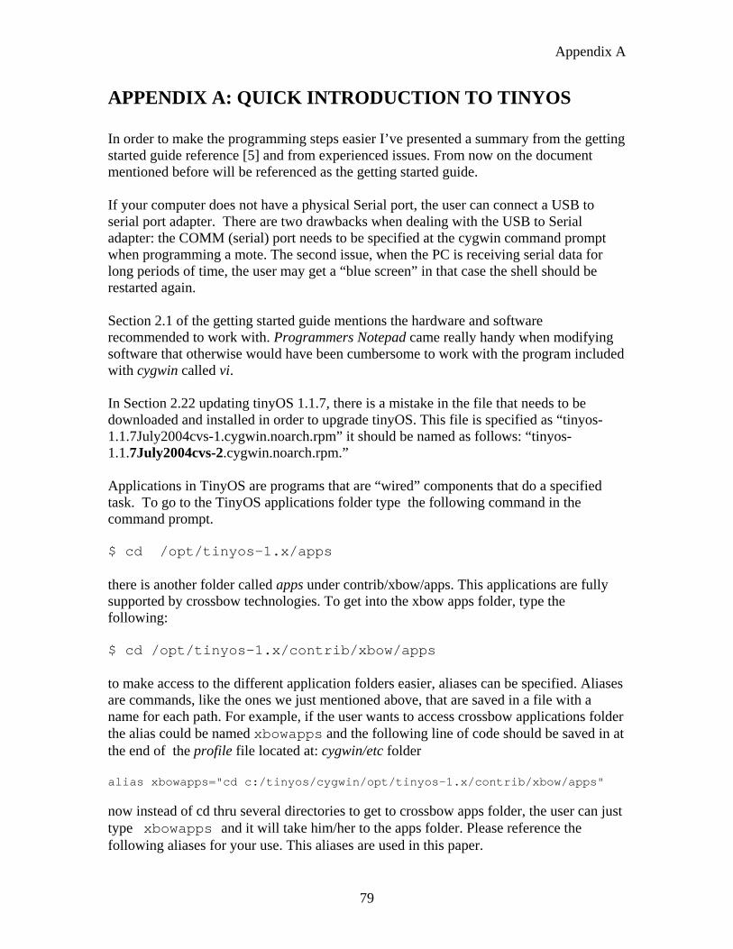
Appendix A
79
APPENDIX A: QUICK INTRODUCTION TO TINYOS In order to make the programming steps easier I’ve presented a summary from the getting started guide reference [5] and from experienced issues. From now on the document mentioned before will be referenced as the getting started guide. If your computer does not have a physical Serial port, the user can connect a USB to serial port adapter. There are two drawbacks when dealing with the USB to Serial adapter: the COMM (serial) port needs to be specified at the cygwin command prompt when programming a mote. The second issue, when the PC is receiving serial data for long periods of time, the user may get a “blue screen” in that case the shell should be restarted again. Section 2.1 of the getting started guide mentions the hardware and software recommended to work with. Programmers Notepad came really handy when modifying software that otherwise would have been cumbersome to work with the program included with cygwin called vi. In Section 2.22 updating tinyOS 1.1.7, there is a mistake in the file that needs to be downloaded and installed in order to upgrade tinyOS. This file is specified as “tinyos-1.1.7July2004cvs-1.cygwin.noarch.rpm” it should be named as follows: “tinyos-1.1.7July2004cvs-2.cygwin.noarch.rpm.” Applications in TinyOS are programs that are “wired” components that do a specified task. To go to the TinyOS applications folder type the following command in the command prompt. $ cd /opt/tinyos-1.x/apps there is another folder called apps under contrib/xbow/apps. This applications are fully supported by crossbow technologies. To get into the xbow apps folder, type the following: $ cd /opt/tinyos-1.x/contrib/xbow/apps to make access to the different application folders easier, aliases can be specified. Aliases are commands, like the ones we just mentioned above, that are saved in a file with a name for each path. For example, if the user wants to access crossbow applications folder the alias could be named xbowapps and the following line of code should be saved in at the end of the profile file located at: cygwin/etc folder alias xbowapps="cd c:/tinyos/cygwin/opt/tinyos-1.x/contrib/xbow/apps" now instead of cd thru several directories to get to crossbow apps folder, the user can just type xbowapps and it will take him/her to the apps folder. Please reference the following aliases for your use. This aliases are used in this paper.
Appendix A
80
Aliases alias cdt="cd c:/tinyos/cygwin/opt/tinyos-1.x" alias xbowapps="cd c:/tinyos/cygwin/opt/tinyos-1.x/contrib/xbow/apps" alias cdxlisten="cd c:/tinyos/cygwin/opt/tinyos-1.x/contrib/xbow/tools/src/xlisten" alias xbowapps="cd c:/tinyos/cygwin/opt/tinyos-1.x/contrib/xbow/apps" alias tosbaseap="cd c:/tinyos/cygwin/opt/tinyos-1.x/contrib/xbow/apps/TOSBase" alias apps="cd c:/tinyos/cygwin/opt/tinyos-1.x/apps" alias xmda="cd c:/tinyos/cygwin/opt/tinyos-1.x/contrib/xbow/apps/XSensorMDA300" alias xsensor="cd c:/tinyos/cygwin/opt/tinyos-1.x/contrib/xbow/apps/XSensorMTS300" alias xgps="cd c:/tinyos/cygwin/opt/tinyos-1.x/contrib/xbow/apps/XSensorMTS400" The following figure shows the file structure for TinyOS. Figure A-1: TinyOS File structure.

Appendix A
81
Programming a mote To program a mote , get into the application folder that you want to program either by cd commands or by typing an alias previously setup, and type the following $ Make mica2 install.# mib510.com# install.# sets the mote ID and com# set the communication port in which the MIB510 programmer board is connected. For example. $ make mica2 install.0 mib510.com4 The user can specify the programmer board and communications port in a bash file in that case, the following should be typed: $ make mica2 install.0 In this case the mote ID is =0 which means is the base station. The rest of the commands where specified in a bash file. For example mib510 and com4. For more information on application installation and options please look at the getting started guide.
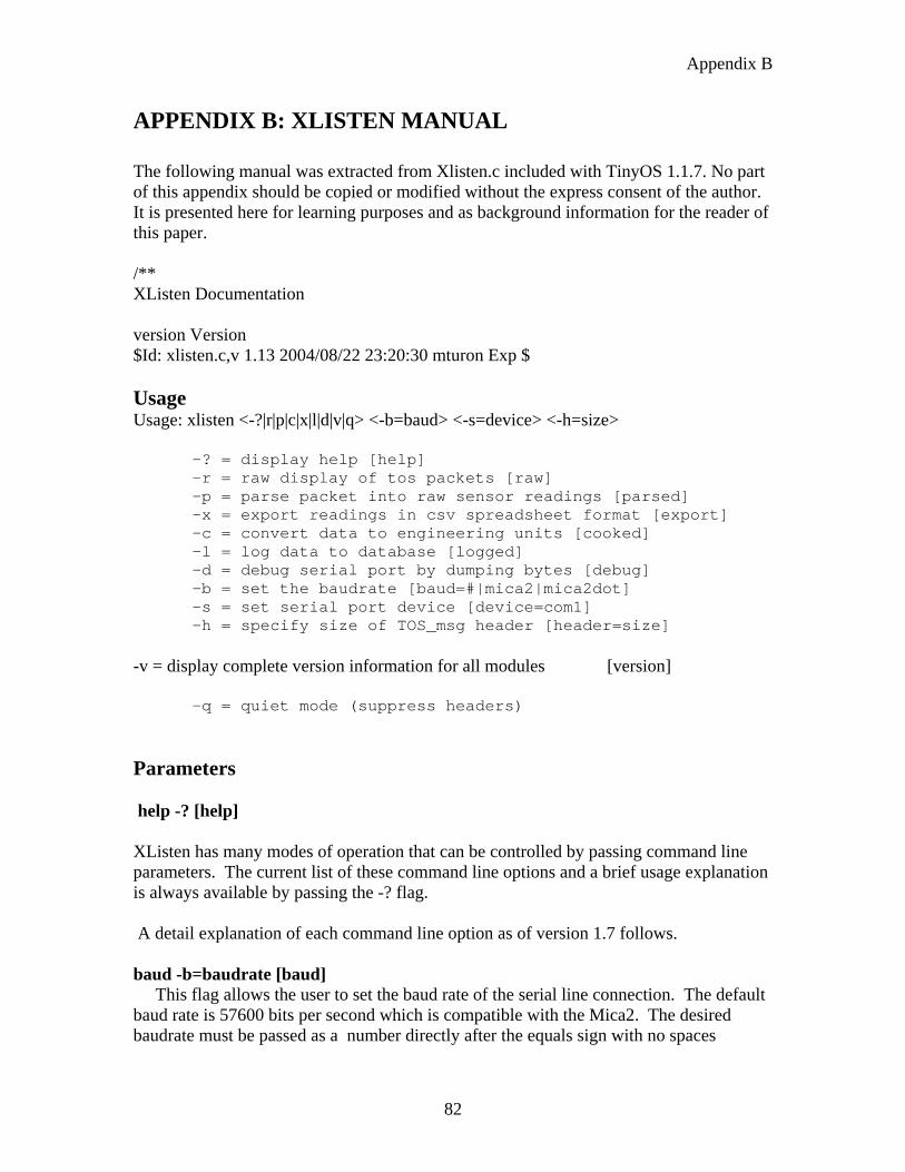
Appendix B
82
APPENDIX B: XLISTEN MANUAL The following manual was extracted from Xlisten.c included with TinyOS 1.1.7. No part of this appendix should be copied or modified without the express consent of the author. It is presented here for learning purposes and as background information for the reader of this paper. /** XListen Documentation version Version $Id: xlisten.c,v 1.13 2004/08/22 23:20:30 mturon Exp $ Usage Usage: xlisten <-?|r|p|c|x|l|d|v|q> <-b=baud> <-s=device> <-h=size> -? = display help [help] -r = raw display of tos packets [raw] -p = parse packet into raw sensor readings [parsed] -x = export readings in csv spreadsheet format [export] -c = convert data to engineering units [cooked] -l = log data to database [logged] -d = debug serial port by dumping bytes [debug] -b = set the baudrate [baud=#|mica2|mica2dot] -s = set serial port device [device=com1] -h = specify size of TOS_msg header [header=size]
-v = display complete version information for all modules [version]
-q = quiet mode (suppress headers) Parameters help -? [help] XListen has many modes of operation that can be controlled by passing command line parameters. The current list of these command line options and a brief usage explanation is always available by passing the -? flag. A detail explanation of each command line option as of version 1.7 follows. baud -b=baudrate [baud] This flag allows the user to set the baud rate of the serial line connection. The default baud rate is 57600 bits per second which is compatible with the Mica2. The desired baudrate must be passed as a number directly after the equals sign with no spaces
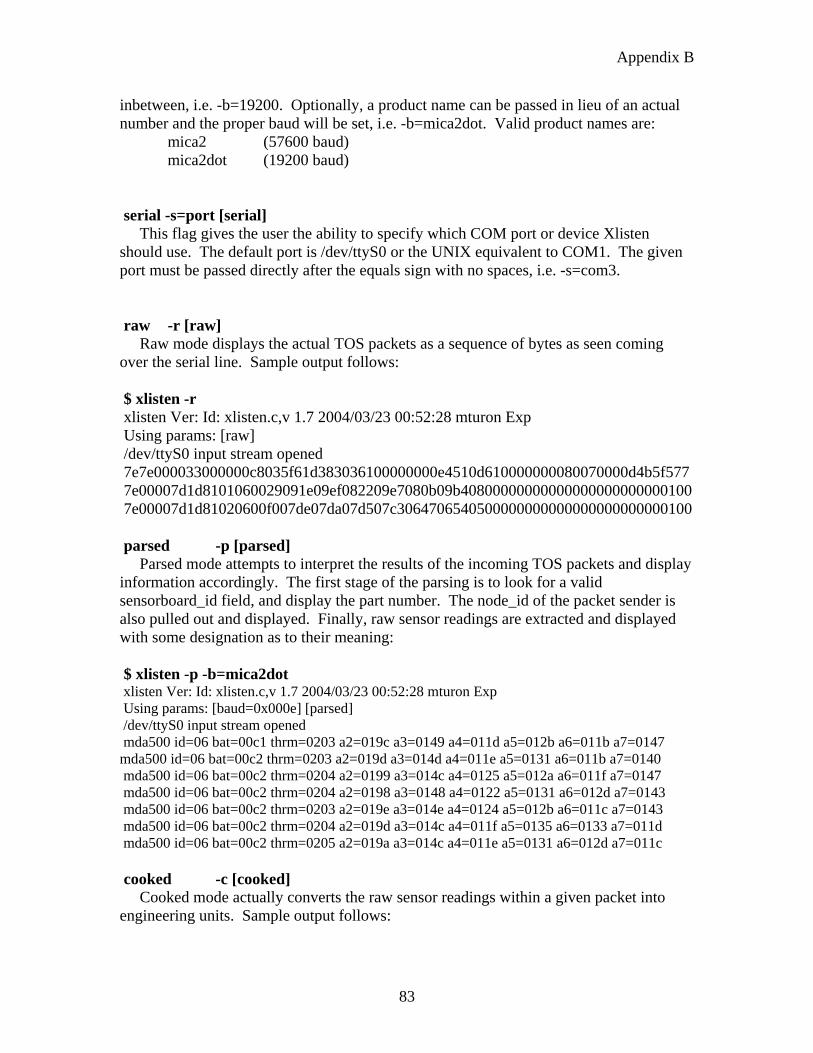
Appendix B
83
inbetween, i.e. -b=19200. Optionally, a product name can be passed in lieu of an actual number and the proper baud will be set, i.e. -b=mica2dot. Valid product names are: mica2 (57600 baud) mica2dot (19200 baud) serial -s=port [serial] This flag gives the user the ability to specify which COM port or device Xlisten should use. The default port is /dev/ttyS0 or the UNIX equivalent to COM1. The given port must be passed directly after the equals sign with no spaces, i.e. -s=com3. raw -r [raw] Raw mode displays the actual TOS packets as a sequence of bytes as seen coming over the serial line. Sample output follows: $ xlisten -r xlisten Ver: Id: xlisten.c,v 1.7 2004/03/23 00:52:28 mturon Exp Using params: [raw] /dev/ttyS0 input stream opened 7e7e000033000000c8035f61d383036100000000e4510d610000000080070000d4b5f577 7e00007d1d8101060029091e09ef082209e7080b09b40800000000000000000000000100 7e00007d1d81020600f007de07da07d507c3064706540500000000000000000000000100 parsed -p [parsed] Parsed mode attempts to interpret the results of the incoming TOS packets and display information accordingly. The first stage of the parsing is to look for a valid sensorboard_id field, and display the part number. The node_id of the packet sender is also pulled out and displayed. Finally, raw sensor readings are extracted and displayed with some designation as to their meaning: $ xlisten -p -b=mica2dot xlisten Ver: Id: xlisten.c,v 1.7 2004/03/23 00:52:28 mturon Exp Using params: [baud=0x000e] [parsed] /dev/ttyS0 input stream opened mda500 id=06 bat=00c1 thrm=0203 a2=019c a3=0149 a4=011d a5=012b a6=011b a7=0147 mda500 id=06 bat=00c2 thrm=0203 a2=019d a3=014d a4=011e a5=0131 a6=011b a7=0140 mda500 id=06 bat=00c2 thrm=0204 a2=0199 a3=014c a4=0125 a5=012a a6=011f a7=0147 mda500 id=06 bat=00c2 thrm=0204 a2=0198 a3=0148 a4=0122 a5=0131 a6=012d a7=0143 mda500 id=06 bat=00c2 thrm=0203 a2=019e a3=014e a4=0124 a5=012b a6=011c a7=0143 mda500 id=06 bat=00c2 thrm=0204 a2=019d a3=014c a4=011f a5=0135 a6=0133 a7=011d mda500 id=06 bat=00c2 thrm=0205 a2=019a a3=014c a4=011e a5=0131 a6=012d a7=011c cooked -c [cooked] Cooked mode actually converts the raw sensor readings within a given packet into engineering units. Sample output follows:
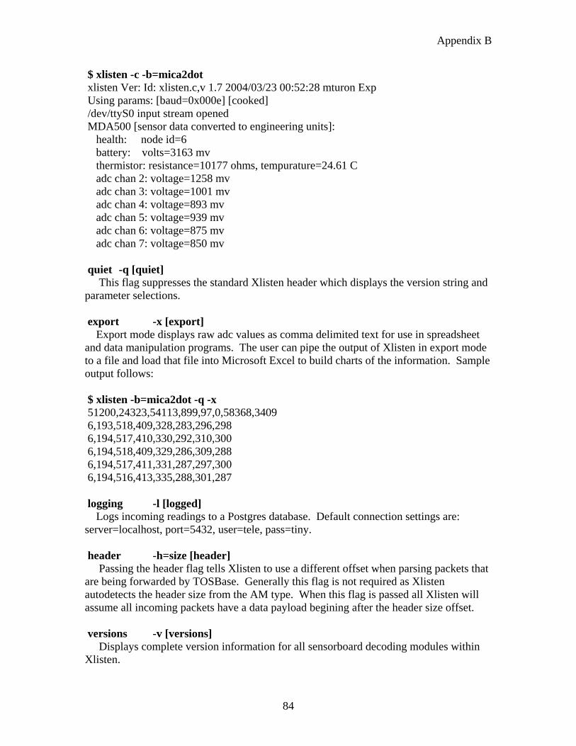
Appendix B
84
$ xlisten -c -b=mica2dot xlisten Ver: Id: xlisten.c,v 1.7 2004/03/23 00:52:28 mturon Exp Using params: [baud=0x000e] [cooked] /dev/ttyS0 input stream opened MDA500 [sensor data converted to engineering units]: health: node id=6 battery: volts=3163 mv thermistor: resistance=10177 ohms, tempurature=24.61 C adc chan 2: voltage=1258 mv adc chan 3: voltage=1001 mv adc chan 4: voltage=893 mv adc chan 5: voltage=939 mv adc chan 6: voltage=875 mv adc chan 7: voltage=850 mv quiet -q [quiet] This flag suppresses the standard Xlisten header which displays the version string and parameter selections. export -x [export] Export mode displays raw adc values as comma delimited text for use in spreadsheet and data manipulation programs. The user can pipe the output of Xlisten in export mode to a file and load that file into Microsoft Excel to build charts of the information. Sample output follows: $ xlisten -b=mica2dot -q -x 51200,24323,54113,899,97,0,58368,3409 6,193,518,409,328,283,296,298 6,194,517,410,330,292,310,300 6,194,518,409,329,286,309,288 6,194,517,411,331,287,297,300 6,194,516,413,335,288,301,287 logging -l [logged] Logs incoming readings to a Postgres database. Default connection settings are: server=localhost, port=5432, user=tele, pass=tiny. header -h=size [header] Passing the header flag tells Xlisten to use a different offset when parsing packets that are being forwarded by TOSBase. Generally this flag is not required as Xlisten autodetects the header size from the AM type. When this flag is passed all Xlisten will assume all incoming packets have a data payload begining after the header size offset. versions -v [versions] Displays complete version information for all sensorboard decoding modules within Xlisten.
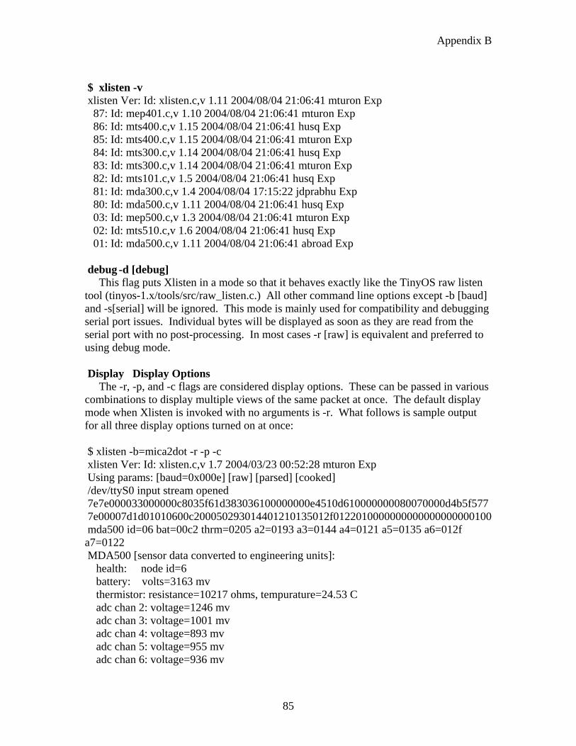
Appendix B
85
$ xlisten -v xlisten Ver: Id: xlisten.c,v 1.11 2004/08/04 21:06:41 mturon Exp 87: Id: mep401.c,v 1.10 2004/08/04 21:06:41 mturon Exp 86: Id: mts400.c,v 1.15 2004/08/04 21:06:41 husq Exp 85: Id: mts400.c,v 1.15 2004/08/04 21:06:41 mturon Exp 84: Id: mts300.c,v 1.14 2004/08/04 21:06:41 husq Exp 83: Id: mts300.c,v 1.14 2004/08/04 21:06:41 mturon Exp 82: Id: mts101.c,v 1.5 2004/08/04 21:06:41 husq Exp 81: Id: mda300.c,v 1.4 2004/08/04 17:15:22 jdprabhu Exp 80: Id: mda500.c,v 1.11 2004/08/04 21:06:41 husq Exp 03: Id: mep500.c,v 1.3 2004/08/04 21:06:41 mturon Exp 02: Id: mts510.c,v 1.6 2004/08/04 21:06:41 husq Exp 01: Id: mda500.c,v 1.11 2004/08/04 21:06:41 abroad Exp debug -d [debug] This flag puts Xlisten in a mode so that it behaves exactly like the TinyOS raw listen tool (tinyos-1.x/tools/src/raw_listen.c.) All other command line options except -b [baud] and -s[serial] will be ignored. This mode is mainly used for compatibility and debugging serial port issues. Individual bytes will be displayed as soon as they are read from the serial port with no post-processing. In most cases -r [raw] is equivalent and preferred to using debug mode. Display Display Options The -r, -p, and -c flags are considered display options. These can be passed in various combinations to display multiple views of the same packet at once. The default display mode when Xlisten is invoked with no arguments is -r. What follows is sample output for all three display options turned on at once: $ xlisten -b=mica2dot -r -p -c xlisten Ver: Id: xlisten.c,v 1.7 2004/03/23 00:52:28 mturon Exp Using params: [baud=0x000e] [raw] [parsed] [cooked] /dev/ttyS0 input stream opened 7e7e000033000000c8035f61d383036100000000e4510d610000000080070000d4b5f577 7e00007d1d01010600c200050293014401210135012f0122010000000000000000000100 mda500 id=06 bat=00c2 thrm=0205 a2=0193 a3=0144 a4=0121 a5=0135 a6=012f a7=0122 MDA500 [sensor data converted to engineering units]: health: node id=6 battery: volts=3163 mv thermistor: resistance=10217 ohms, tempurature=24.53 C adc chan 2: voltage=1246 mv adc chan 3: voltage=1001 mv adc chan 4: voltage=893 mv adc chan 5: voltage=955 mv adc chan 6: voltage=936 mv
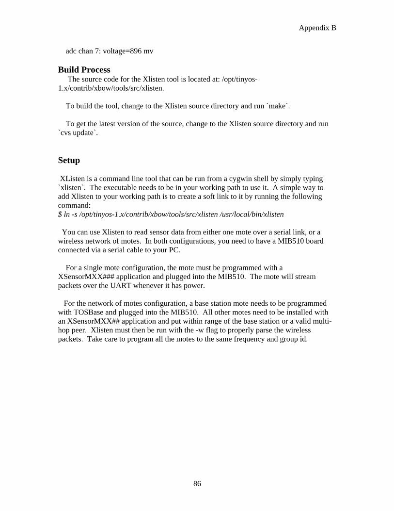
Appendix B
86
adc chan 7: voltage=896 mv Build Process The source code for the Xlisten tool is located at: /opt/tinyos-1.x/contrib/xbow/tools/src/xlisten. To build the tool, change to the Xlisten source directory and run `make`. To get the latest version of the source, change to the Xlisten source directory and run `cvs update`. Setup XListen is a command line tool that can be run from a cygwin shell by simply typing `xlisten`. The executable needs to be in your working path to use it. A simple way to add Xlisten to your working path is to create a soft link to it by running the following command: $ ln -s /opt/tinyos-1.x/contrib/xbow/tools/src/xlisten /usr/local/bin/xlisten You can use Xlisten to read sensor data from either one mote over a serial link, or a wireless network of motes. In both configurations, you need to have a MIB510 board connected via a serial cable to your PC. For a single mote configuration, the mote must be programmed with a XSensorMXX### application and plugged into the MIB510. The mote will stream packets over the UART whenever it has power. For the network of motes configuration, a base station mote needs to be programmed with TOSBase and plugged into the MIB510. All other motes need to be installed with an XSensorMXX## application and put within range of the base station or a valid multi-hop peer. Xlisten must then be run with the -w flag to properly parse the wireless packets. Take care to program all the motes to the same frequency and group id.
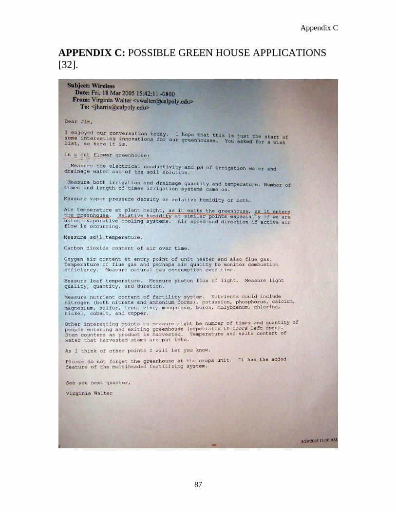
Appendix C
87
APPENDIX C: POSSIBLE GREEN HOUSE APPLICATIONS [32].
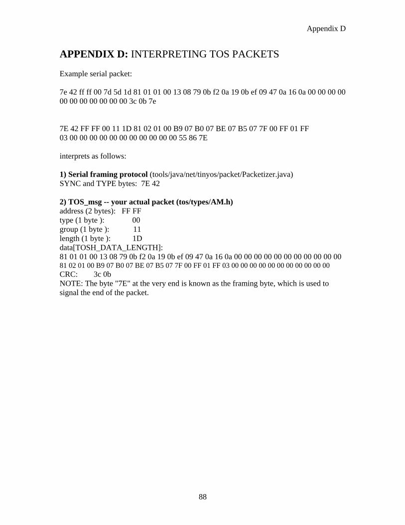
Appendix D
88
APPENDIX D: INTERPRETING TOS PACKETS Example serial packet: 7e 42 ff ff 00 7d 5d 1d 81 01 01 00 13 08 79 0b f2 0a 19 0b ef 09 47 0a 16 0a 00 00 00 00 00 00 00 00 00 00 00 3c 0b 7e 7E 42 FF FF 00 11 1D 81 02 01 00 B9 07 B0 07 BE 07 B5 07 7F 00 FF 01 FF 03 00 00 00 00 00 00 00 00 00 00 00 55 86 7E interprets as follows: 1) Serial framing protocol (tools/java/net/tinyos/packet/Packetizer.java) SYNC and TYPE bytes: 7E 42 2) TOS_msg -- your actual packet (tos/types/AM.h) address (2 bytes): FF FF type (1 byte ): 00 group (1 byte ): 11 length (1 byte ): 1D data[TOSH_DATA_LENGTH]: 81 01 01 00 13 08 79 0b f2 0a 19 0b ef 09 47 0a 16 0a 00 00 00 00 00 00 00 00 00 00 00 81 02 01 00 B9 07 B0 07 BE 07 B5 07 7F 00 FF 01 FF 03 00 00 00 00 00 00 00 00 00 00 00 CRC: 3c 0b NOTE: The byte "7E" at the very end is known as the framing byte, which is used to signal the end of the packet.
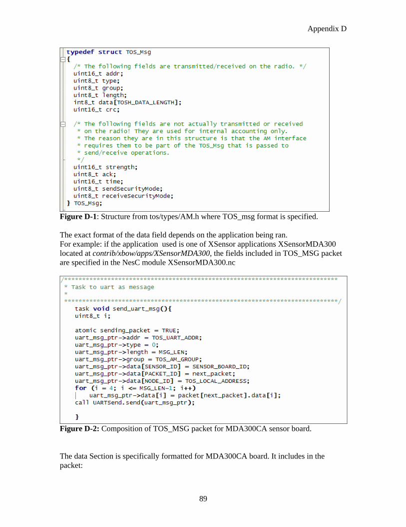
Appendix D
89
Figure D-1: Structure from tos/types/AM.h where TOS_msg format is specified. The exact format of the data field depends on the application being ran. For example: if the application used is one of XSensor applications XSensorMDA300 located at contrib/xbow/apps/XSensorMDA300, the fields included in TOS_MSG packet are specified in the NesC module XSensorMDA300.nc
Figure D-2: Composition of TOS_MSG packet for MDA300CA sensor board. The data Section is specifically formatted for MDA300CA board. It includes in the packet:
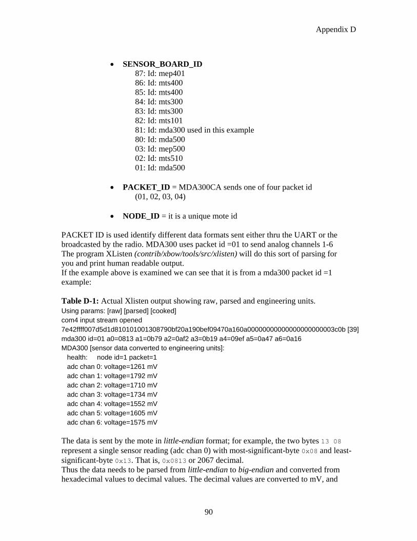
Appendix D
90
• SENSOR_BOARD_ID
87: Id: mep401 86: Id: mts400 85: Id: mts400 84: Id: mts300 83: Id: mts300 82: Id: mts101 81: Id: mda300 used in this example 80: Id: mda500 03: Id: mep500 02: Id: mts510 01: Id: mda500
• PACKET_ID = MDA300CA sends one of four packet id (01, 02, 03, 04)
• NODE_ID = it is a unique mote id PACKET ID is used identify different data formats sent either thru the UART or the broadcasted by the radio. MDA300 uses packet id =01 to send analog channels 1-6 The program XListen (contrib/xbow/tools/src/xlisten) will do this sort of parsing for you and print human readable output. If the example above is examined we can see that it is from a mda300 packet id =1 example: Table D-1: Actual Xlisten output showing raw, parsed and engineering units. Using params: [raw] [parsed] [cooked] com4 input stream opened 7e42ffff007d5d1d810101001308790bf20a190bef09470a160a00000000000000000000003c0b [39]mda300 id=01 a0=0813 a1=0b79 a2=0af2 a3=0b19 a4=09ef a5=0a47 a6=0a16 MDA300 [sensor data converted to engineering units]: health: node id=1 packet=1 adc chan 0: voltage=1261 mV adc chan 1: voltage=1792 mV adc chan 2: voltage=1710 mV adc chan 3: voltage=1734 mV adc chan 4: voltage=1552 mV adc chan 5: voltage=1605 mV adc chan 6: voltage=1575 mV The data is sent by the mote in little-endian format; for example, the two bytes 13 08 represent a single sensor reading (adc chan 0) with most-significant-byte 0x08 and least-significant-byte 0x13. That is, 0x0813 or 2067 decimal. Thus the data needs to be parsed from little-endian to big-endian and converted from hexadecimal values to decimal values. The decimal values are converted to mV, and
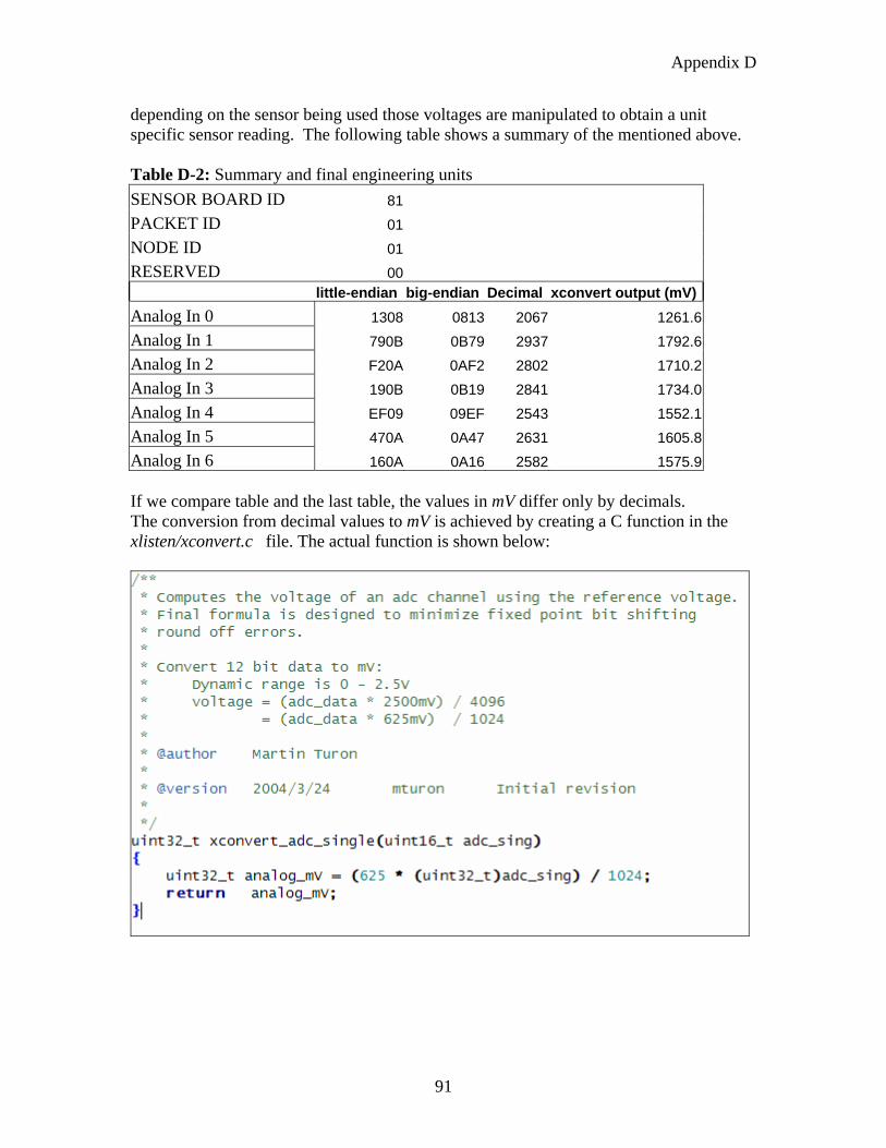
Appendix D
91
depending on the sensor being used those voltages are manipulated to obtain a unit specific sensor reading. The following table shows a summary of the mentioned above. Table D-2: Summary and final engineering units SENSOR BOARD ID 81 PACKET ID 01 NODE ID 01 RESERVED 00 little-endian big-endian Decimal xconvert output (mV) Analog In 0 1308 0813 2067 1261.6 Analog In 1 790B 0B79 2937 1792.6 Analog In 2 F20A 0AF2 2802 1710.2 Analog In 3 190B 0B19 2841 1734.0 Analog In 4 EF09 09EF 2543 1552.1 Analog In 5 470A 0A47 2631 1605.8 Analog In 6 160A 0A16 2582 1575.9 If we compare table and the last table, the values in mV differ only by decimals. The conversion from decimal values to mV is achieved by creating a C function in the xlisten/xconvert.c file. The actual function is shown below:
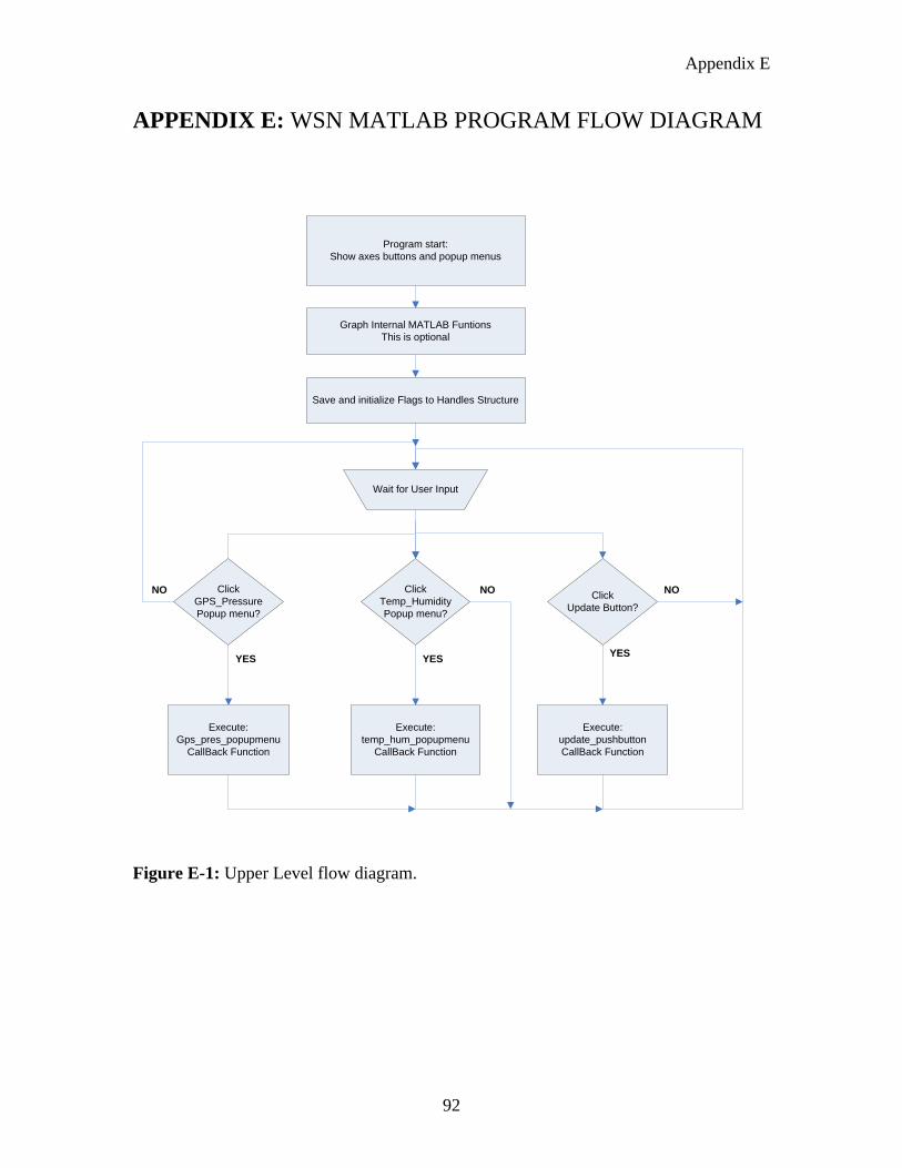
Appendix E
92
APPENDIX E: WSN MATLAB PROGRAM FLOW DIAGRAM
Program start:Show axes buttons and popup menus
Graph Internal MATLAB FuntionsThis is optional
Save and initialize Flags to Handles Structure
Wait for User Input
ClickGPS_PressurePopup menu?
ClickTemp_HumidityPopup menu?
ClickUpdate Button?
Execute:Gps_pres_popupmenu
CallBack Function
Execute:temp_hum_popupmenu
CallBack Function
Execute:update_pushbuttonCallBack Function
YES YES YES
NO NO NO
Figure E-1: Upper Level flow diagram.
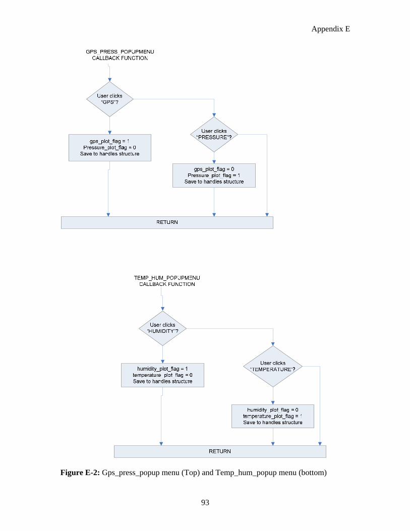
Appendix E
93
Figure E-2: Gps_press_popup menu (Top) and Temp_hum_popup menu (bottom)
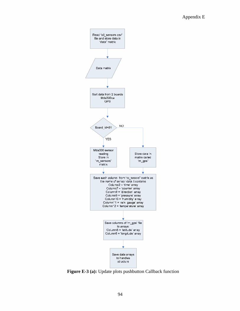
Appendix E
94
Figure E-3 (a): Update plots pushbutton Callback function
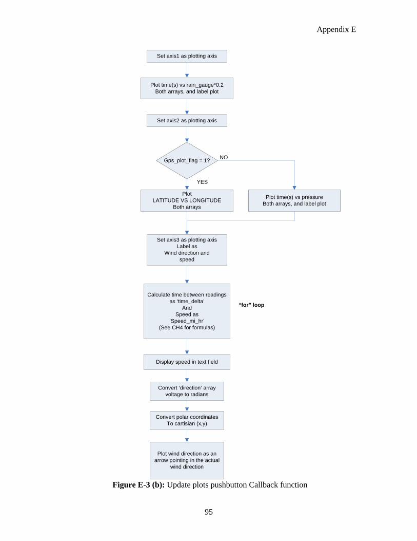
Appendix E
95
Set axis1 as plotting axis
Plot time(s) vs rain_gauge*0.2Both arrays, and label plot
Set axis2 as plotting axis
Plot LATITUDE VS LONGITUDE
Both arrays
Gps_plot_flag = 1?
YES
NO
Plot time(s) vs pressureBoth arrays, and label plot
Set axis3 as plotting axisLabel as
Wind direction andspeed
Calculate time between readings as ‘time_delta’
AndSpeed as
‘Speed_mi_hr’(See CH4 for formulas)
“for” loop
Display speed in text field
Convert ‘direction’ array voltage to radians
Convert polar coordinatesTo cartisian (x,y)
Plot wind direction as an arrow pointing in the actual
wind direction
Figure E-3 (b): Update plots pushbutton Callback function
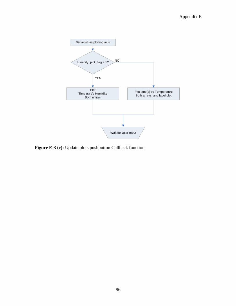
Appendix E
96
Set axis4 as plotting axis
Plot Time (s) Vs Humidity
Both arrays
humidity_plot_flag = 1?
YES
NO
Plot time(s) vs TemperatureBoth arrays, and label plot
Wait for User Input
Figure E-3 (c): Update plots pushbutton Callback function
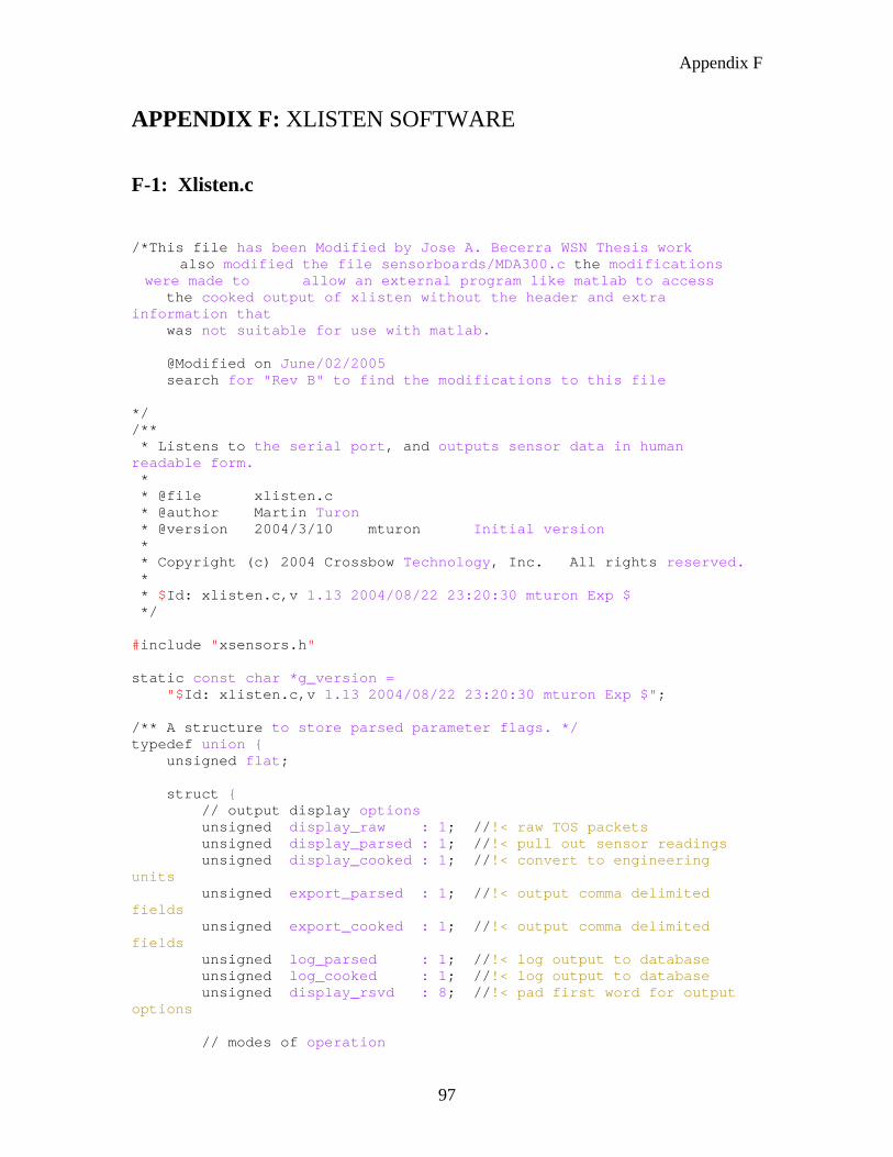
Appendix F
97
APPENDIX F: XLISTEN SOFTWARE F-1: Xlisten.c
/*This file has been Modified by Jose A. Becerra WSN Thesis work also modified the file sensorboards/MDA300.c the modifications were made to allow an external program like matlab to access
the cooked output of xlisten without the header and extra information that was not suitable for use with matlab. @Modified on June/02/2005 search for "Rev B" to find the modifications to this file */ /** * Listens to the serial port, and outputs sensor data in human readable form. * * @file xlisten.c * @author Martin Turon * @version 2004/3/10 mturon Initial version * * Copyright (c) 2004 Crossbow Technology, Inc. All rights reserved. * * $Id: xlisten.c,v 1.13 2004/08/22 23:20:30 mturon Exp $ */ #include "xsensors.h" static const char *g_version = "$Id: xlisten.c,v 1.13 2004/08/22 23:20:30 mturon Exp $"; /** A structure to store parsed parameter flags. */ typedef union { unsigned flat; struct { // output display options unsigned display_raw : 1; //!< raw TOS packets unsigned display_parsed : 1; //!< pull out sensor readings unsigned display_cooked : 1; //!< convert to engineering units unsigned export_parsed : 1; //!< output comma delimited fields unsigned export_cooked : 1; //!< output comma delimited fields unsigned log_parsed : 1; //!< log output to database unsigned log_cooked : 1; //!< log output to database unsigned display_rsvd : 8; //!< pad first word for output options // modes of operation
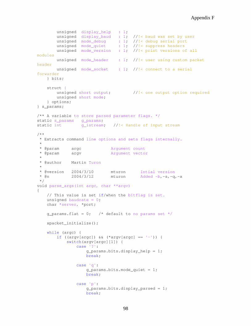
Appendix F
98
unsigned display_help : 1; unsigned display_baud : 1; //!< baud was set by user unsigned mode_debug : 1; //!< debug serial port unsigned mode_quiet : 1; //!< suppress headers unsigned mode_version : 1; //!< print versions of all modules unsigned mode_header : 1; //!< user using custom packet header unsigned mode_socket : 1; //!< connect to a serial forwarder } bits; struct { unsigned short output; //!< one output option required unsigned short mode; } options; } s_params; /** A variable to store parsed parameter flags. */ static s_params g_params; static int g_istream; //!< Handle of input stream /** * Extracts command line options and sets flags internally. * * @param argc Argument count * @param argv Argument vector * * @author Martin Turon * * @version 2004/3/10 mturon Intial version * @n 2004/3/12 mturon Added -b,-s,-q,-x */ void parse_args(int argc, char **argv) { // This value is set if/when the bitflag is set. unsigned baudrate = 0; char *server, *port; g_params.flat = 0; /* default to no params set */ xpacket_initialize(); while (argc) { if ((argv[argc]) && (*argv[argc] == '-')) { switch(argv[argc][1]) { case '?': g_params.bits.display_help = 1; break; case 'q': g_params.bits.mode_quiet = 1; break; case 'p': g_params.bits.display_parsed = 1; break;
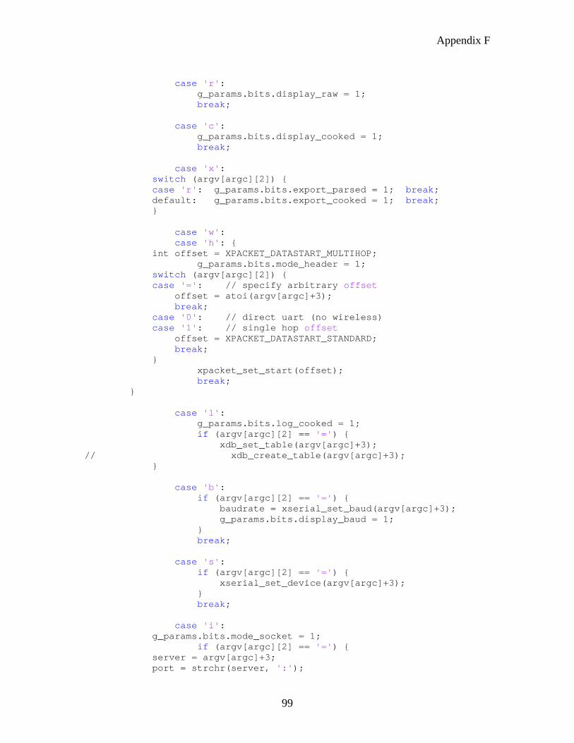
Appendix F
99
case 'r': g_params.bits.display_raw = 1; break; case 'c': g_params.bits.display_cooked = 1; break; case 'x': switch (argv[argc][2]) { case 'r': g_params.bits.export_parsed = 1; break; default: g_params.bits.export_cooked = 1; break; } case 'w': case 'h': { int offset = XPACKET_DATASTART_MULTIHOP; g_params.bits.mode_header = 1; switch (argv[argc][2]) { case '=': // specify arbitrary offset offset = atoi(argv[argc]+3); break; case '0': // direct uart (no wireless) case '1': // single hop offset offset = XPACKET_DATASTART_STANDARD; break; } xpacket_set_start(offset); break; } case 'l': g_params.bits.log_cooked = 1; if (argv[argc][2] == '=') { xdb_set_table(argv[argc]+3); // xdb_create_table(argv[argc]+3); } case 'b': if (argv[argc][2] == '=') { baudrate = xserial_set_baud(argv[argc]+3); g_params.bits.display_baud = 1; } break; case 's': if (argv[argc][2] == '=') { xserial_set_device(argv[argc]+3); } break; case 'i': g_params.bits.mode_socket = 1; if (argv[argc][2] == '=') { server = argv[argc]+3; port = strchr(server, ':');
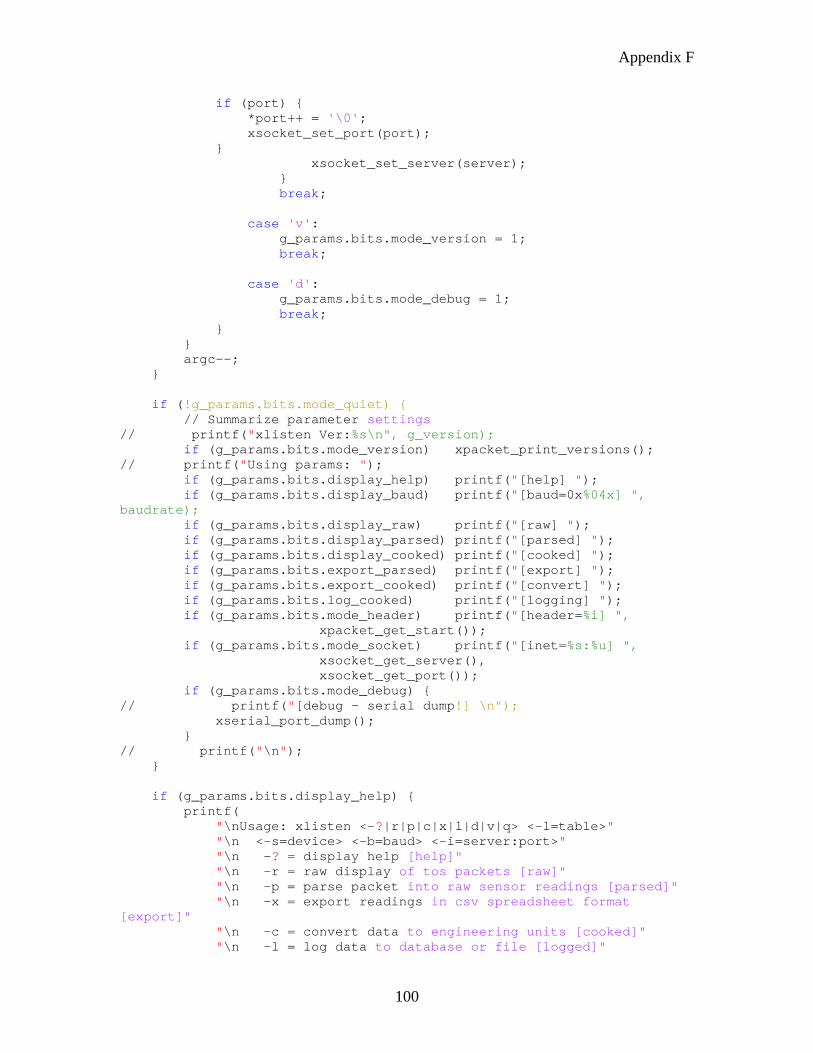
Appendix F
100
if (port) { *port++ = '\0'; xsocket_set_port(port); } xsocket_set_server(server); } break; case 'v': g_params.bits.mode_version = 1; break; case 'd': g_params.bits.mode_debug = 1; break; } } argc--; } if (!g_params.bits.mode_quiet) { // Summarize parameter settings // printf("xlisten Ver:%s\n", g_version); if (g_params.bits.mode_version) xpacket_print_versions(); // printf("Using params: "); if (g_params.bits.display_help) printf("[help] "); if (g_params.bits.display_baud) printf("[baud=0x%04x] ", baudrate); if (g_params.bits.display_raw) printf("[raw] "); if (g_params.bits.display_parsed) printf("[parsed] "); if (g_params.bits.display_cooked) printf("[cooked] "); if (g_params.bits.export_parsed) printf("[export] "); if (g_params.bits.export_cooked) printf("[convert] "); if (g_params.bits.log_cooked) printf("[logging] "); if (g_params.bits.mode_header) printf("[header=%i] ", xpacket_get_start()); if (g_params.bits.mode_socket) printf("[inet=%s:%u] ", xsocket_get_server(), xsocket_get_port()); if (g_params.bits.mode_debug) { // printf("[debug - serial dump!] \n"); xserial_port_dump(); } // printf("\n"); } if (g_params.bits.display_help) { printf( "\nUsage: xlisten <-?|r|p|c|x|l|d|v|q> <-l=table>" "\n <-s=device> <-b=baud> <-i=server:port>" "\n -? = display help [help]" "\n -r = raw display of tos packets [raw]" "\n -p = parse packet into raw sensor readings [parsed]" "\n -x = export readings in csv spreadsheet format [export]" "\n -c = convert data to engineering units [cooked]" "\n -l = log data to database or file [logged]"
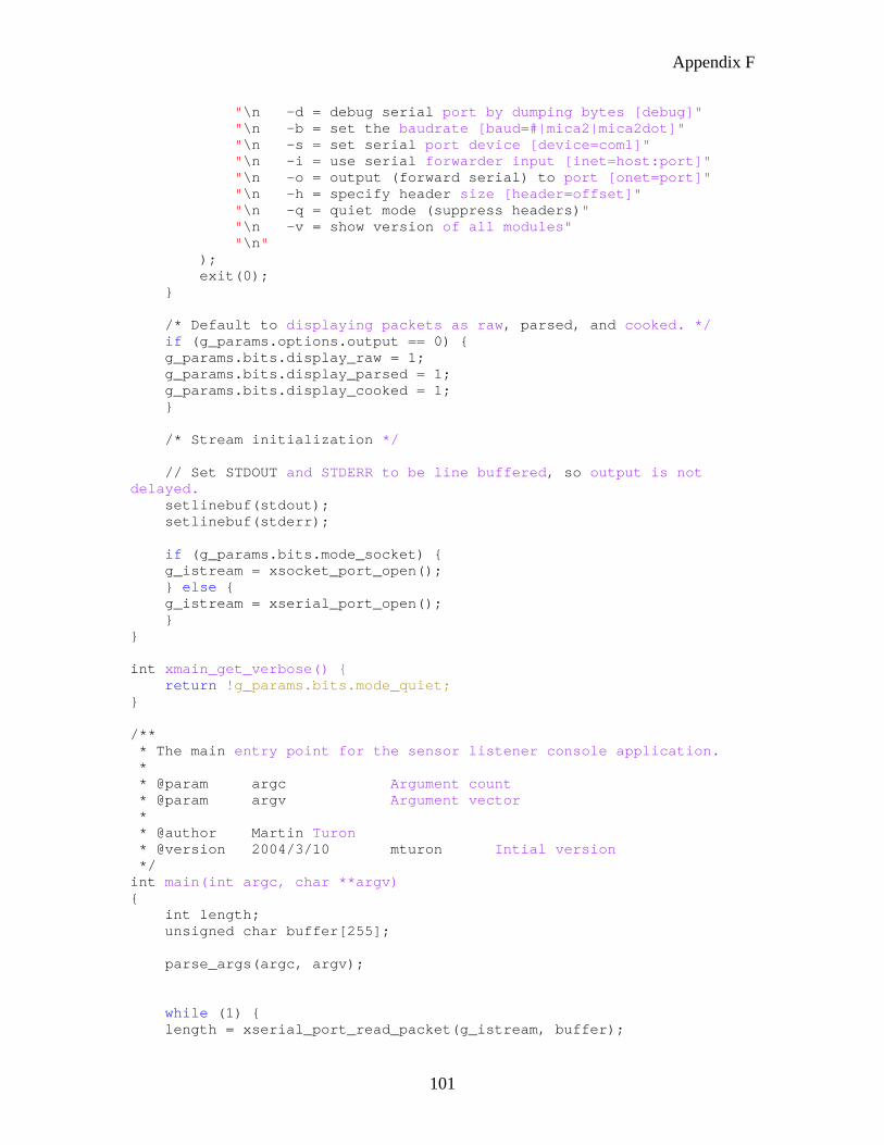
Appendix F
101
"\n -d = debug serial port by dumping bytes [debug]" "\n -b = set the baudrate [baud=#|mica2|mica2dot]" "\n -s = set serial port device [device=com1]" "\n -i = use serial forwarder input [inet=host:port]" "\n -o = output (forward serial) to port [onet=port]" "\n -h = specify header size [header=offset]" "\n -q = quiet mode (suppress headers)" "\n -v = show version of all modules" "\n" ); exit(0); } /* Default to displaying packets as raw, parsed, and cooked. */ if (g_params.options.output == 0) { g_params.bits.display_raw = 1; g_params.bits.display_parsed = 1; g_params.bits.display_cooked = 1; } /* Stream initialization */ // Set STDOUT and STDERR to be line buffered, so output is not delayed. setlinebuf(stdout); setlinebuf(stderr); if (g_params.bits.mode_socket) { g_istream = xsocket_port_open(); } else { g_istream = xserial_port_open(); } } int xmain_get_verbose() { return !g_params.bits.mode_quiet; } /** * The main entry point for the sensor listener console application. * * @param argc Argument count * @param argv Argument vector * * @author Martin Turon * @version 2004/3/10 mturon Intial version */ int main(int argc, char **argv) { int length; unsigned char buffer[255]; parse_args(argc, argv); while (1) { length = xserial_port_read_packet(g_istream, buffer);
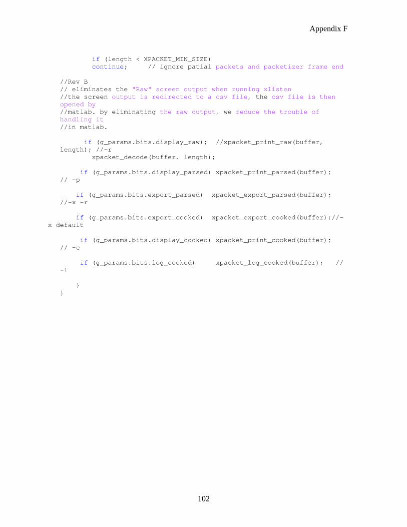
Appendix F
102
if (length < XPACKET_MIN_SIZE) continue; // ignore patial packets and packetizer frame end //Rev B // eliminates the "Raw" screen output when running xlisten //the screen output is redirected to a csv file, the csv file is then opened by //matlab. by eliminating the raw output, we reduce the trouble of handling it //in matlab. if (g_params.bits.display_raw); //xpacket_print_raw(buffer, length); //-r xpacket_decode(buffer, length); if (g_params.bits.display_parsed) xpacket_print_parsed(buffer); // -p if (g_params.bits.export_parsed) xpacket_export_parsed(buffer); //-x -r
if (g_params.bits.export_cooked) xpacket_export_cooked(buffer);//-x default
if (g_params.bits.display_cooked) xpacket_print_cooked(buffer); // -c if (g_params.bits.log_cooked) xpacket_log_cooked(buffer); // -l } }
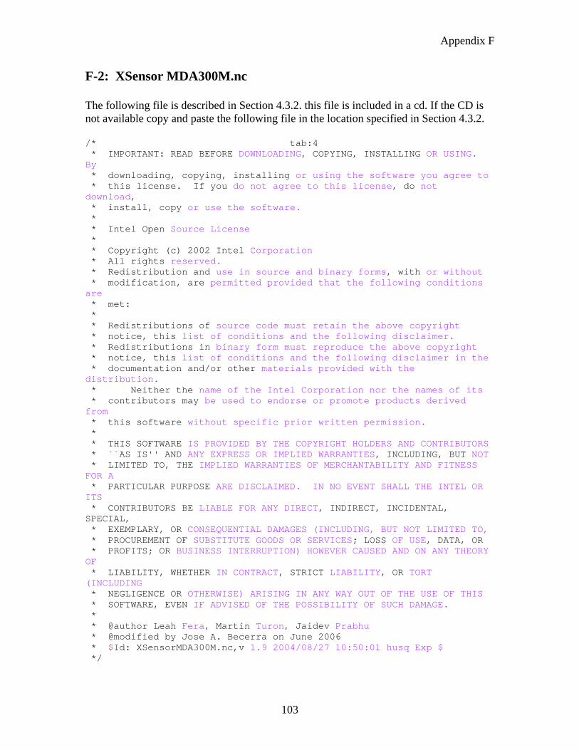
Appendix F
103
F-2: XSensor MDA300M.nc
The following file is described in Section 4.3.2. this file is included in a cd. If the CD is not available copy and paste the following file in the location specified in Section 4.3.2. /* tab:4 * IMPORTANT: READ BEFORE DOWNLOADING, COPYING, INSTALLING OR USING. By * downloading, copying, installing or using the software you agree to * this license. If you do not agree to this license, do not download, * install, copy or use the software. * * Intel Open Source License * * Copyright (c) 2002 Intel Corporation * All rights reserved. * Redistribution and use in source and binary forms, with or without * modification, are permitted provided that the following conditions are * met: * * Redistributions of source code must retain the above copyright * notice, this list of conditions and the following disclaimer. * Redistributions in binary form must reproduce the above copyright * notice, this list of conditions and the following disclaimer in the * documentation and/or other materials provided with the distribution. * Neither the name of the Intel Corporation nor the names of its * contributors may be used to endorse or promote products derived from * this software without specific prior written permission. * * THIS SOFTWARE IS PROVIDED BY THE COPYRIGHT HOLDERS AND CONTRIBUTORS * ``AS IS'' AND ANY EXPRESS OR IMPLIED WARRANTIES, INCLUDING, BUT NOT * LIMITED TO, THE IMPLIED WARRANTIES OF MERCHANTABILITY AND FITNESS FOR A * PARTICULAR PURPOSE ARE DISCLAIMED. IN NO EVENT SHALL THE INTEL OR ITS * CONTRIBUTORS BE LIABLE FOR ANY DIRECT, INDIRECT, INCIDENTAL, SPECIAL, * EXEMPLARY, OR CONSEQUENTIAL DAMAGES (INCLUDING, BUT NOT LIMITED TO, * PROCUREMENT OF SUBSTITUTE GOODS OR SERVICES; LOSS OF USE, DATA, OR * PROFITS; OR BUSINESS INTERRUPTION) HOWEVER CAUSED AND ON ANY THEORY OF * LIABILITY, WHETHER IN CONTRACT, STRICT LIABILITY, OR TORT (INCLUDING * NEGLIGENCE OR OTHERWISE) ARISING IN ANY WAY OUT OF THE USE OF THIS * SOFTWARE, EVEN IF ADVISED OF THE POSSIBILITY OF SUCH DAMAGE. * * @author Leah Fera, Martin Turon, Jaidev Prabhu * @modified by Jose A. Becerra on June 2006 * $Id: XSensorMDA300M.nc,v 1.9 2004/08/27 10:50:01 husq Exp $ */
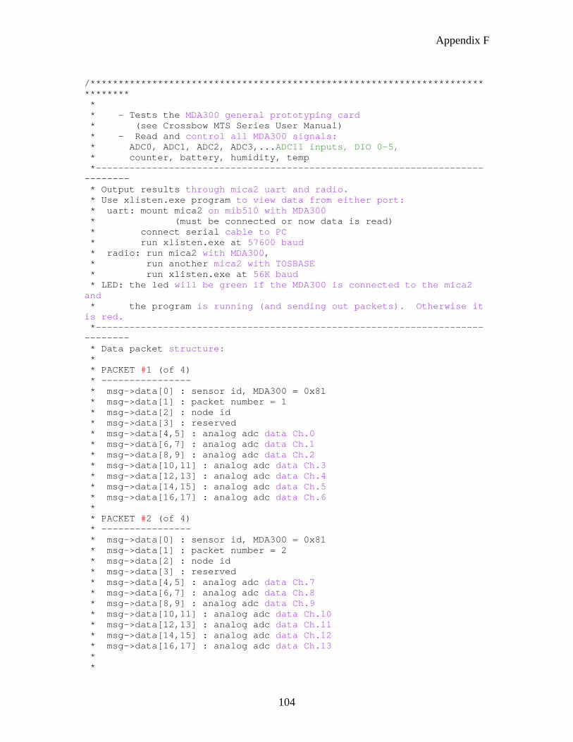
Appendix F
104
/****************************************************************************** * * - Tests the MDA300 general prototyping card * (see Crossbow MTS Series User Manual) * - Read and control all MDA300 signals: * ADC0, ADC1, ADC2, ADC3,...ADC11 inputs, DIO 0-5, * counter, battery, humidity, temp *----------------------------------------------------------------------------- * Output results through mica2 uart and radio. * Use xlisten.exe program to view data from either port: * uart: mount mica2 on mib510 with MDA300 * (must be connected or now data is read) * connect serial cable to PC * run xlisten.exe at 57600 baud * radio: run mica2 with MDA300, * run another mica2 with TOSBASE * run xlisten.exe at 56K baud * LED: the led will be green if the MDA300 is connected to the mica2 and * the program is running (and sending out packets). Otherwise it is red. *----------------------------------------------------------------------------- * Data packet structure: * * PACKET #1 (of 4) * ---------------- * msg->data[0] : sensor id, MDA300 = 0x81 * msg->data[1] : packet number = 1 * msg->data[2] : node id * msg->data[3] : reserved * msg->data[4,5] : analog adc data Ch.0 * msg->data[6,7] : analog adc data Ch.1 * msg->data[8,9] : analog adc data Ch.2 * msg->data[10,11] : analog adc data Ch.3 * msg->data[12,13] : analog adc data Ch.4 * msg->data[14,15] : analog adc data Ch.5 * msg->data[16,17] : analog adc data Ch.6 * * PACKET #2 (of 4) * ---------------- * msg->data[0] : sensor id, MDA300 = 0x81 * msg->data[1] : packet number = 2 * msg->data[2] : node id * msg->data[3] : reserved * msg->data[4,5] : analog adc data Ch.7 * msg->data[6,7] : analog adc data Ch.8 * msg->data[8,9] : analog adc data Ch.9 * msg->data[10,11] : analog adc data Ch.10 * msg->data[12,13] : analog adc data Ch.11 * msg->data[14,15] : analog adc data Ch.12 * msg->data[16,17] : analog adc data Ch.13 * *
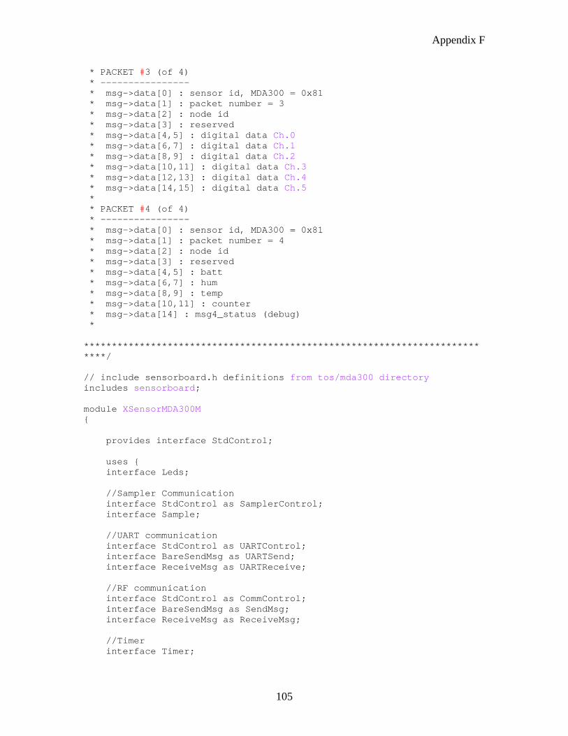
Appendix F
105
* PACKET #3 (of 4) * ---------------- * msg->data[0] : sensor id, MDA300 = 0x81 * msg->data[1] : packet number = 3 * msg->data[2] : node id * msg->data[3] : reserved * msg->data[4,5] : digital data Ch.0 * msg->data[6,7] : digital data Ch.1 * msg->data[8,9] : digital data Ch.2 * msg->data[10,11] : digital data Ch.3 * msg->data[12,13] : digital data Ch.4 * msg->data[14,15] : digital data Ch.5 * * PACKET #4 (of 4) * ---------------- * msg->data[0] : sensor id, MDA300 = 0x81 * msg->data[1] : packet number = 4 * msg->data[2] : node id * msg->data[3] : reserved * msg->data[4,5] : batt * msg->data[6,7] : hum * msg->data[8,9] : temp * msg->data[10,11] : counter * msg->data[14] : msg4_status (debug) * ***************************************************************************/ // include sensorboard.h definitions from tos/mda300 directory includes sensorboard; module XSensorMDA300M { provides interface StdControl; uses { interface Leds; //Sampler Communication interface StdControl as SamplerControl; interface Sample; //UART communication interface StdControl as UARTControl; interface BareSendMsg as UARTSend; interface ReceiveMsg as UARTReceive; //RF communication interface StdControl as CommControl; interface BareSendMsg as SendMsg; interface ReceiveMsg as ReceiveMsg; //Timer interface Timer;
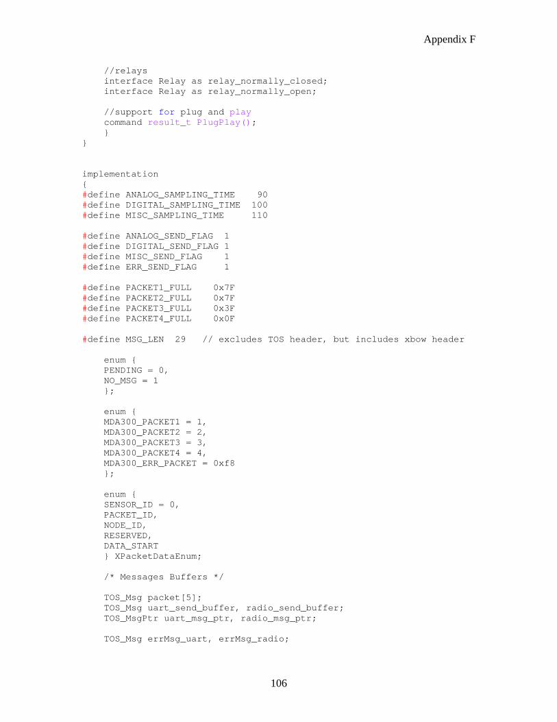
Appendix F
106
//relays interface Relay as relay_normally_closed; interface Relay as relay_normally_open; //support for plug and play command result_t PlugPlay(); } } implementation { #define ANALOG_SAMPLING_TIME 90 #define DIGITAL_SAMPLING_TIME 100 #define MISC_SAMPLING_TIME 110 #define ANALOG_SEND_FLAG 1 #define DIGITAL_SEND_FLAG 1 #define MISC_SEND_FLAG 1 #define ERR_SEND_FLAG 1 #define PACKET1_FULL 0x7F #define PACKET2_FULL 0x7F #define PACKET3_FULL 0x3F #define PACKET4_FULL 0x0F #define MSG_LEN 29 // excludes TOS header, but includes xbow header enum { PENDING = 0, NO_MSG = 1 }; enum { MDA300_PACKET1 = 1, MDA300_PACKET2 = 2, MDA300_PACKET3 = 3, MDA300_PACKET4 = 4, MDA300_ERR_PACKET = 0xf8 }; enum { SENSOR_ID = 0, PACKET_ID, NODE_ID, RESERVED, DATA_START } XPacketDataEnum; /* Messages Buffers */ TOS_Msg packet[5]; TOS_Msg uart_send_buffer, radio_send_buffer; TOS_MsgPtr uart_msg_ptr, radio_msg_ptr; TOS_Msg errMsg_uart, errMsg_radio;
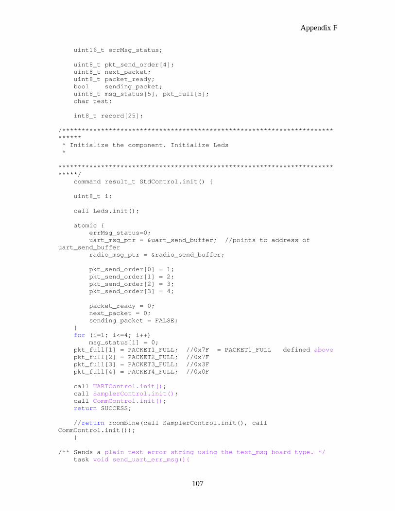
Appendix F
107
uint16_t errMsg_status; uint8_t pkt_send_order[4]; uint8_t next_packet; uint8_t packet_ready; bool sending_packet; uint8_t msg_status[5], pkt_full[5]; char test; int8_t record[25]; /**************************************************************************** * Initialize the component. Initialize Leds * ****************************************************************************/ command result_t StdControl.init() { uint8_t i; call Leds.init(); atomic { errMsg_status=0; uart_msg_ptr = &uart_send_buffer; //points to address of uart_send_buffer radio_msg_ptr = &radio_send_buffer; pkt_send_order[0] = 1; pkt_send_order[1] = 2; pkt_send_order[2] = 3; pkt_send_order[3] = 4; packet_ready = 0; next_packet = 0; sending_packet = FALSE; } for (i=1; i<=4; i++) msg_status[i] = 0; pkt_full[1] = PACKET1_FULL; //0x7F = PACKET1_FULL defined above pkt_full[2] = PACKET2_FULL; //0x7F pkt_full[3] = PACKET3_FULL; //0x3F pkt_full[4] = PACKET4_FULL; //0x0F call UARTControl.init(); call SamplerControl.init(); call CommControl.init(); return SUCCESS; //return rcombine(call SamplerControl.init(), call CommControl.init()); } /** Sends a plain text error string using the text_msg board type. */ task void send_uart_err_msg(){
Appendix F
108
uint8_t i; char *errMsg = "mda300 not found"; errMsg_status = 1 && ERR_SEND_FLAG; if (!errMsg_status) return; //if the ERR_SEND_FLAG is not =1 (there is no error) //return to program flow errMsg_uart.data[SENSOR_ID] = SENSOR_BOARD_ID; errMsg_uart.data[PACKET_ID] = MDA300_ERR_PACKET; errMsg_uart.data[NODE_ID] = TOS_LOCAL_ADDRESS; errMsg_uart.addr = TOS_UART_ADDR; errMsg_uart.type = 0; errMsg_uart.length = MSG_LEN; //TOSH_DATA_LENGTH; errMsg_uart.group = TOS_AM_GROUP; i = 0; // Copy error string while ((*errMsg) && (i <= MSG_LEN-1)) { errMsg_uart.data[DATA_START + i] = errMsg[i]; i++; } // Copy over uart packet to radio packet (identical) for (i = 0; i <= MSG_LEN-1; i++) errMsg_radio.data[i] = errMsg_uart.data[i]; call UARTSend.send(&errMsg_uart); } /**************************************************************************** * Start the component. Start the clock. Setup timer and sampling * ****************************************************************************/ command result_t StdControl.start() { call UARTControl.start(); call SamplerControl.start(); call CommControl.start(); if(call PlugPlay()) { call Timer.start(TIMER_REPEAT, 3000); //channel parameteres are irrelevent //int8_t getSample(uint8_t channel, uint8_t channelType, uint16_t interval, uint8_t param) record[14] = call Sample.getSample(0,TEMPERATURE,MISC_SAMPLING_TIME,SAMPLER_DEFAULT);
Appendix F
109
record[15] = call Sample.getSample(0,HUMIDITY,MISC_SAMPLING_TIME,SAMPLER_DEFAULT); record[16] = call Sample.getSample(0, BATTERY,MISC_SAMPLING_TIME,SAMPLER_DEFAULT); //start sampling channels. Channels 7-10 with averaging since they are more percise.channels 3-6 make active excitation //record[0] = call Sample.getSample(0,ANALOG,ANALOG_SAMPLING_TIME,SAMPLER_DEFAULT | EXCITATION_33); record[0] = call Sample.getSample(0, COUNTER,ANALOG_SAMPLING_TIME,RESET_ZERO_AFTER_READ | RISING_EDGE); //COUNTER (ANALOG 0) record[1] = call Sample.getSample(1,ANALOG,ANALOG_SAMPLING_TIME,EXCITATION_25 ); //DIRECTION (ANALOG 1) //record[2] = call Sample.getSample(2,ANALOG,ANALOG_SAMPLING_TIME,SAMPLER_DEFAULT); record[2] = call Sample.getSample(2,ANALOG,ANALOG_SAMPLING_TIME,EXCITATION_50 | DELAY_BEFORE_MEASUREMENT); // PRESURE (ANALOG 2) //record[3] = call Sample.getSample(3,ANALOG,ANALOG_SAMPLING_TIME,SAMPLER_DEFAULT | EXCITATION_33 | DELAY_BEFORE_MEASUREMENT); //Humidity Sensor connected to ADC3 record[3] = call Sample.getSample(3,ANALOG,ANALOG_SAMPLING_TIME,EXCITATION_33 | DELAY_BEFORE_MEASUREMENT | AVERAGE_FOUR); //HUMIDITY (ANALOG 3) //record[4] = call Sample.getSample(4,ANALOG,ANALOG_SAMPLING_TIME,SAMPLER_DEFAULT); record[4] = call Sample.getSample(1,DIGITAL,ANALOG_SAMPLING_TIME,RISING_EDGE | EEPROM_TOTALIZER); //RAIN FALL COUNT record[5] = call Sample.getSample(5,ANALOG,ANALOG_SAMPLING_TIME,SAMPLER_DEFAULT); record[6] = call Sample.getSample(6,ANALOG,ANALOG_SAMPLING_TIME,EXCITATION_25); //EXT TEMPERATURE record[7] = call Sample.getSample(7,ANALOG,ANALOG_SAMPLING_TIME,AVERAGE_FOUR | EXCITATION_25); record[8] = call Sample.getSample(8,ANALOG,ANALOG_SAMPLING_TIME,AVERAGE_FOUR | EXCITATION_25);
Appendix F
110
record[9] = call Sample.getSample(9,ANALOG,ANALOG_SAMPLING_TIME,AVERAGE_FOUR | EXCITATION_25); record[10] = call Sample.getSample(10,ANALOG,ANALOG_SAMPLING_TIME,AVERAGE_FOUR | EXCITATION_25); record[11] = call Sample.getSample(11,ANALOG,ANALOG_SAMPLING_TIME,SAMPLER_DEFAULT); record[12] = call Sample.getSample(12,ANALOG,ANALOG_SAMPLING_TIME,SAMPLER_DEFAULT); record[13] = call Sample.getSample(13,ANALOG,ANALOG_SAMPLING_TIME,SAMPLER_DEFAULT | EXCITATION_50 | EXCITATION_ALWAYS_ON); //digital chennels as accumulative counter record[17] = call Sample.getSample(0,DIGITAL,DIGITAL_SAMPLING_TIME,RESET_ZERO_AFTER_READ | FALLING_EDGE); //record[18] = call Sample.getSample(1,DIGITAL,DIGITAL_SAMPLING_TIME,RISING_EDGE | EVENT); record[18] = call Sample.getSample(4,ANALOG,ANALOG_SAMPLING_TIME,SAMPLER_DEFAULT); record[19] = call Sample.getSample(2,DIGITAL,DIGITAL_SAMPLING_TIME,SAMPLER_DEFAULT | EVENT); record[20] = call Sample.getSample(3,DIGITAL,DIGITAL_SAMPLING_TIME,FALLING_EDGE); record[21] = call Sample.getSample(4,DIGITAL,DIGITAL_SAMPLING_TIME,RISING_EDGE); record[22] = call Sample.getSample(5,DIGITAL,DIGITAL_SAMPLING_TIME,RISING_EDGE | EEPROM_TOTALIZER); //counter channels for frequency measurement, will reset to zero. record[23] = call Sample.getSample(0,ANALOG,ANALOG_SAMPLING_TIME,SAMPLER_DEFAULT | EXCITATION_33); //record[23] = call Sample.getSample(0, COUNTER,MISC_SAMPLING_TIME,RESET_ZERO_AFTER_READ | RISING_EDGE); call Leds.greenOn(); }
Appendix F
111
else { post send_uart_err_msg(); call Leds.redOn(); } return SUCCESS; } /**************************************************************************** * Stop the component. * ****************************************************************************/ command result_t StdControl.stop() { call SamplerControl.stop(); return SUCCESS; } /**************************************************************************** * Task to uart as message * ****************************************************************************/ task void send_uart_msg(){ uint8_t i; atomic sending_packet = TRUE; uart_msg_ptr->addr = TOS_UART_ADDR; uart_msg_ptr->type = 0; uart_msg_ptr->length = MSG_LEN; uart_msg_ptr->group = TOS_AM_GROUP; uart_msg_ptr->data[SENSOR_ID] = SENSOR_BOARD_ID; uart_msg_ptr->data[PACKET_ID] = next_packet; uart_msg_ptr->data[NODE_ID] = TOS_LOCAL_ADDRESS; for (i = 4; i <= MSG_LEN-1; i++) uart_msg_ptr->data[i] = packet[next_packet].data[i]; call UARTSend.send(uart_msg_ptr); } /**************************************************************************** * Task to transmit radio message * NOTE that data payload was already copied from the corresponding UART packet
Appendix F
112
****************************************************************************/ task void send_radio_msg() { uint8_t i; radio_msg_ptr->addr = TOS_BCAST_ADDR; radio_msg_ptr->type = 0; radio_msg_ptr->length = MSG_LEN; //TOSH_DATA_LENGTH; radio_msg_ptr->group = TOS_AM_GROUP; radio_msg_ptr->data[SENSOR_ID] = SENSOR_BOARD_ID; radio_msg_ptr->data[PACKET_ID] = next_packet; radio_msg_ptr->data[NODE_ID] = TOS_LOCAL_ADDRESS; for (i = 4; i <= MSG_LEN-1; i++) radio_msg_ptr->data[i] = packet[next_packet].data[i]; // call SendMsg.send(TOS_BCAST_ADDR, MSG_LEN, radio_msg_ptr); call SendMsg.send(radio_msg_ptr); } /**************************************************************************** * Uart msg xmitted. * Transmit same msg over radio ****************************************************************************/ event result_t UARTSend.sendDone(TOS_MsgPtr msg, result_t success) { uart_msg_ptr = msg; call Leds.yellowOn(); post send_radio_msg(); return SUCCESS; } /**************************************************************************** * Radio msg xmitted. ****************************************************************************/ event result_t SendMsg.sendDone(TOS_MsgPtr msg, result_t success) { radio_msg_ptr = msg; call Leds.yellowOff(); // mark that this packet has been sent atomic { sending_packet = FALSE; packet_ready &= ~(1 << (next_packet - 1)); } return SUCCESS; }
Appendix F
113
/**************************************************************************** * Radio msg rcvd. * This app doesn't respond to any incoming radio msg * Just return ****************************************************************************/ event TOS_MsgPtr ReceiveMsg.receive(TOS_MsgPtr data) { return data; } /**************************************************************************** * Uart msg rcvd. * This app doesn't respond to any incoming uart msg * Just return ****************************************************************************/ event TOS_MsgPtr UARTReceive.receive(TOS_MsgPtr data) { return data; } /** * Handle a single dataReady event for all MDA300 data types. * * @author Leah Fera, Martin Turon * * @version 2004/3/17 leahfera Intial revision * @n 2004/4/1 mturon Improved state machine * @n 2006/7/23 Jose becerra custom application */ event result_t Sample.dataReady(uint8_t channel,uint8_t channelType,uint16_t data) { uint8_t i; switch (channelType) { case ANALOG: switch (channel) { // MSG 1 : first part of analog channels (0-6) case 0: //packet[1].data[DATA_START+0]=data & 0xff; //packet[1].data[DATA_START+1]=(data >> 8) & 0xff; //packet[1].data[DATA_START+0]=data & 0xff; //packet[1].data[DATA_START+1]=(data >> 8) & 0xff; atomic {msg_status[1] |=0x00;} break; case 1: packet[1].data[DATA_START+2]=data & 0xff; packet[1].data[DATA_START+3]=(data >> 8) & 0xff; atomic {msg_status[1] |=0x02;} break;
Appendix F
114
case 2: packet[1].data[DATA_START+4]=data & 0xff; packet[1].data[DATA_START+5]=(data >> 8) & 0xff; atomic {msg_status[1] |=0x04;} break; case 3: packet[1].data[DATA_START+6]=data & 0xff; packet[1].data[DATA_START+7]=(data >> 8) & 0xff; atomic {msg_status[1] |=0x08;} break; case 4: //packet[1].data[DATA_START+8]=data & 0xff; //packet[1].data[DATA_START+9]=(data >> 8) & 0xff; //atomic {msg_status[1] |=0x10;} atomic {msg_status[1] |=0x00;} break; case 5: //packet[1].data[DATA_START+10]=data & 0xff; //packet[1].data[DATA_START+11]=(data >> 8) & 0xff; //atomic {msg_status[1] |=0x20;} atomic {msg_status[1] |=0x00;} break; case 6: packet[1].data[DATA_START+12]=data & 0xff; packet[1].data[DATA_START+13]=(data >> 8) & 0xff; atomic {msg_status[1]|=0x40;} break; // MSG 2 : second part of analog channels (7-13) case 7: packet[2].data[DATA_START+0]=data & 0xff; packet[2].data[DATA_START+1]=(data >> 8) & 0xff; atomic {msg_status[2]|=0x01;} break; case 8: packet[2].data[DATA_START+2]=data & 0xff; packet[2].data[DATA_START+3]=(data >> 8) & 0xff; atomic {msg_status[2]|=0x02;} break; case 9: packet[2].data[DATA_START+4]=data & 0xff; packet[2].data[DATA_START+5]=(data >> 8) & 0xff; atomic {msg_status[2]|=0x04;} break; case 10: packet[2].data[DATA_START+6]=data & 0xff; packet[2].data[DATA_START+7]=(data >> 8) & 0xff; atomic {msg_status[2]|=0x08;}
Appendix F
115
break; case 11: packet[2].data[DATA_START+8]=data & 0xff; packet[2].data[DATA_START+9]=(data >> 8) & 0xff; atomic {msg_status[2]|=0x10;} break; case 12: packet[2].data[DATA_START+10]=data & 0xff; packet[2].data[DATA_START+11]=(data >> 8) & 0xff; atomic {msg_status[2]|=0x20;} break; case 13: packet[2].data[DATA_START+12]=data & 0xff; packet[2].data[DATA_START+13]=(data >> 8) & 0xff; atomic {msg_status[2]|=0x40;} break; default: break; } // case ANALOG (channel) break; case DIGITAL: switch (channel) { case 0: packet[3].data[2]=data & 0xff; packet[3].data[3]=(data >> 8) & 0xff; atomic {msg_status[3]|=0x01;} break; case 1: //packet[3].data[4]=data & 0xff; //packet[3].data[5]=(data >> 8) & 0xff; //atomic {msg_status[3]|=0x02;} //Dig 1 shows up at Analog4 packet[1].data[DATA_START+8]=data & 0xff; packet[1].data[DATA_START+9]=(data >> 8) & 0xff; atomic {msg_status[1] |=0x10;} break; case 2: packet[3].data[6]=data & 0xff; packet[3].data[7]=(data >> 8) & 0xff; atomic {msg_status[3]|=0x04;} break; case 3: packet[3].data[8]=data & 0xff; packet[3].data[9]=(data >> 8) & 0xff; atomic {msg_status[3]|=0x08;} break; case 4:
Appendix F
116
packet[3].data[10]=data & 0xff; packet[3].data[11]=(data >> 8) & 0xff; atomic {msg_status[3]|=0x10;} break; case 5: packet[3].data[12]=data & 0xff; packet[3].data[13]=(data >> 8) & 0xff; atomic {msg_status[3]|=0x20;} break; default: break; } // case DIGITAL (channel) break; case BATTERY: packet[4].data[4]=data & 0xff; packet[4].data[5]=(data >> 8) & 0xff; atomic {msg_status[4]|=0x01;} break; case HUMIDITY: packet[4].data[6]=data & 0xff; packet[4].data[7]=(data >> 8) & 0xff; atomic {msg_status[4]|=0x02;} break; case TEMPERATURE: //packet[4].data[8]=data & 0xff; //packet[4].data[9]=(data >> 8) & 0xff; //atomic {msg_status[4]|=0x04;} packet[1].data[DATA_START+10]=data & 0xff; packet[1].data[DATA_START+11]=(data >> 8) & 0xff; atomic {msg_status[1] |=0x20;} break; case COUNTER: //packet[4].data[10]=data & 0xff; //packet[4].data[11]=(data >> 8) & 0xff; //atomic {msg_status[4]|=0x08;} packet[1].data[DATA_START+0]=data & 0xff; packet[1].data[DATA_START+1]=(data >> 8) & 0xff; atomic {msg_status[1]|=0x01;} break; default: break; } // switch (channelType) atomic { for (i=1; i<=4; i++) { if (sending_packet) // avoid posting uart_send-Task while one is in process break;
Appendix F
117
next_packet = pkt_send_order[0]; pkt_send_order[0] = pkt_send_order[1]; pkt_send_order[1] = pkt_send_order[2]; pkt_send_order[2] = pkt_send_order[3]; pkt_send_order[3] = next_packet; if (msg_status[next_packet] == pkt_full[next_packet]) { msg_status[next_packet] = 0; packet_ready |= 1 << (next_packet - 1); post send_uart_msg(); break; } } } return SUCCESS; } /**************************************************************************** * Timer Fired - * ****************************************************************************/ event result_t Timer.fired() { if (test != 0) { test=0; call relay_normally_closed.toggle(); } else { test=1; call relay_normally_open.toggle(); } return SUCCESS; } }
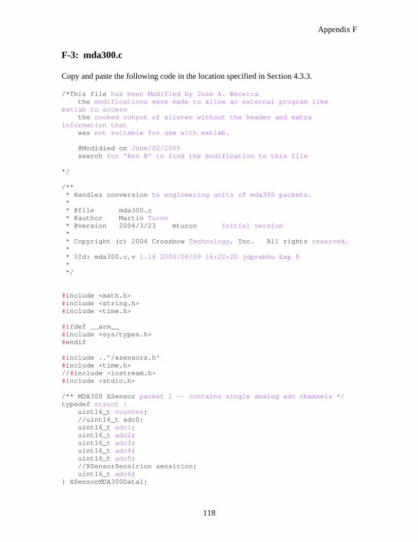
Appendix F
118
F-3: mda300.c
Copy and paste the following code in the location specified in Section 4.3.3. /*This file has been Modified by Jose A. Becerra the modifications were made to allow an external program like matlab to access the cooked output of xlisten without the header and extra information that was not suitable for use with matlab. @Modidied on June/02/2005 search for "Rev B" to find the modification to this file */ /** * Handles conversion to engineering units of mda300 packets. * * @file mda300.c * @author Martin Turon * @version 2004/3/23 mturon Initial version * * Copyright (c) 2004 Crossbow Technology, Inc. All rights reserved. * * $Id: mda300.c,v 1.18 2004/08/09 16:22:20 jdprabhu Exp $ * */ #include <math.h> #include <string.h> #include <time.h> #ifdef __arm__ #include <sys/types.h> #endif #include ..”/xsensors.h" #include <time.h> //#include <iostream.h> #include <stdio.h> /** MDA300 XSensor packet 1 -- contains single analog adc channels */ typedef struct { uint16_t counter; //uint16_t adc0; uint16_t adc1; uint16_t adc2; uint16_t adc3; uint16_t adc4; uint16_t adc5; //XSensorSensirion sensirion; uint16_t adc6; } XSensorMDA300Data1;
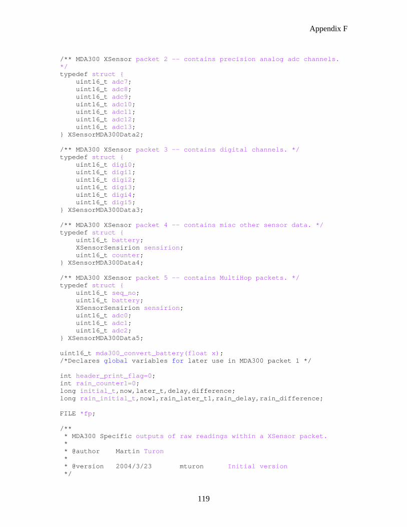
Appendix F
119
/** MDA300 XSensor packet 2 -- contains precision analog adc channels. */ typedef struct { uint16_t adc7; uint16_t adc8; uint16_t adc9; uint16_t adc10; uint16_t adc11; uint16_t adc12; uint16_t adc13; } XSensorMDA300Data2; /** MDA300 XSensor packet 3 -- contains digital channels. */ typedef struct { uint16_t digi0; uint16_t digi1; uint16_t digi2; uint16_t digi3; uint16_t digi4; uint16_t digi5; } XSensorMDA300Data3; /** MDA300 XSensor packet 4 -- contains misc other sensor data. */ typedef struct { uint16_t battery; XSensorSensirion sensirion; uint16_t counter; } XSensorMDA300Data4; /** MDA300 XSensor packet 5 -- contains MultiHop packets. */ typedef struct { uint16_t seq_no; uint16_t battery; XSensorSensirion sensirion; uint16_t adc0; uint16_t adc1; uint16_t adc2; } XSensorMDA300Data5; uint16_t mda300_convert_battery(float x); /*Declares global variables for later use in MDA300 packet 1 */ int header_print_flag=0; int rain_counter1=0; long initial_t,now,later_t,delay,difference; long rain_initial_t,now1,rain_later_t1,rain_delay,rain_difference; FILE *fp; /** * MDA300 Specific outputs of raw readings within a XSensor packet. * * @author Martin Turon * * @version 2004/3/23 mturon Initial version */
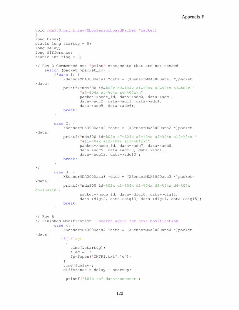
Appendix F
120
void mda300_print_raw(XbowSensorboardPacket *packet) { long time(); static long startup = 0; long delay; long difference; static int flag = 0; // Rev B Commented out "print" statements that are not needed switch (packet->packet_id) { /*case 1: { XSensorMDA300Data1 *data = (XSensorMDA300Data1 *)packet->data; printf("mda300 id=%02x a0=%04x a1=%04x a2=%04x a3=%04x " "a4=%04x a5=%04x a6=%04x\n", packet->node_id, data->adc0, data->adc1, data->adc2, data->adc3, data->adc4, data->adc5, data->adc6); break; } case 2: { XSensorMDA300Data2 *data = (XSensorMDA300Data2 *)packet->data; printf("mda300 id=%02x a7=%04x a8=%04x a9=%04x a10=%04x " "a11=%04x a12=%04x a13=%04x\n", packet->node_id, data->adc7, data->adc8, data->adc9, data->adc10, data->adc11, data->adc12, data->adc13); break; } */ case 3: { XSensorMDA300Data3 *data = (XSensorMDA300Data3 *)packet->data; printf("mda300 id=%02x d1=%04x d2=%04x d3=%04x d4=%04x d5=%04x\n", packet->node_id, data->digi0, data->digi1, data->digi2, data->digi3, data->digi4, data->digi5); break; } // Rev B // Finished Modification --search again for next modification case 4: { XSensorMDA300Data4 *data = (XSensorMDA300Data4 *)packet->data; if(!flag) { time(&startup); flag = 1; fp=fopen("CNTR1.txt","w"); } time(&delay); difference = delay - startup; printf("%04x \n",data->counter);
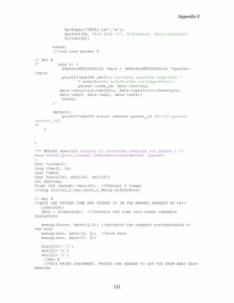
Appendix F
121
fp=fopen("CNTR1.txt","a"); fprintf(fp, "%ld %04x \n", difference, data->counter); fclose(fp); break; }//end case packet 4 // Rev B /* case 5: { XSensorMDA300Data5 *data = (XSensorMDA300Data5 *)packet->data; printf("mda300 id=%02x bat=%04x hum=%04x temp=%04x " " echo10=%04x echo20=%04x soiltemp=%04x\n", packet->node_id, data->battery, data->sensirion.humidity, data->sensirion.thermistor, data->adc0, data->adc1, data->adc2); break; } default: printf("mda300 error: unknown packet_id (%i)\n",packet->packet_id); */ } } /** MDA300 specific display of converted readings for packet 1 */ void mda300_print_cooked_1(XbowSensorboardPacket *packet) { char *ctime(); long time(), tm; char *date; char hours[10], min[10], sec[10]; int mdaflag; float ch6 =packet->data[6]; //Channel 6 (temp) //long initial_t,now,later_t,delay,difference; // Rev B /*gETS THE SYSTEM TIME AND STORES IT IN THE MEMORY ADDRESS OF tm*/ time(&tm); date = ctime(&tm); //converts the time into human readable characters memcpy(hours, date+11,2); //extracts the numbers corresponding to the hour memcpy(min, date+14, 2); //from date memcpy(sec, date+17, 2); hours[2]='\0'; min[2]='\0'; sec[2]='\0'; //Rev B //THIS PRINT STATEMENT, PRINTS THE HEADER TO LET YOU KNOW WHAT EACH READING
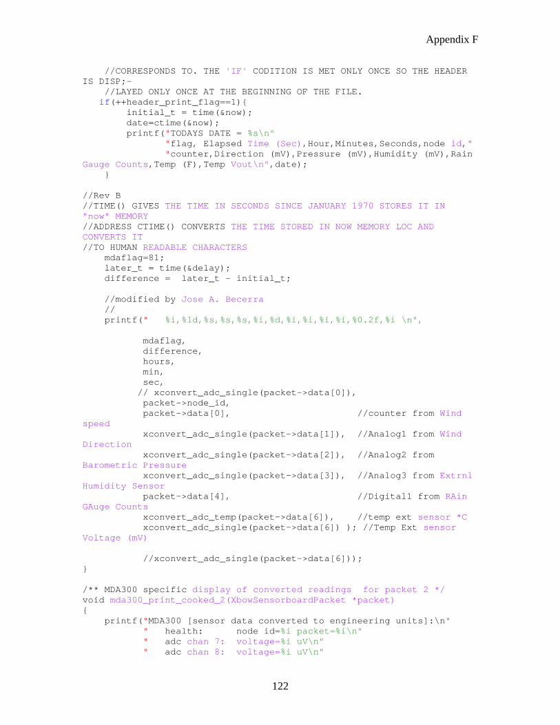
Appendix F
122
//CORRESPONDS TO. THE 'IF' CODITION IS MET ONLY ONCE SO THE HEADER IS DISP;- //LAYED ONLY ONCE AT THE BEGINNING OF THE FILE. if(++header_print_flag==1){ initial_t = time(&now); date=ctime(&now); printf("TODAYS DATE = %s\n" "flag, Elapsed Time (Sec),Hour,Minutes,Seconds,node id," "counter,Direction (mV),Pressure (mV),Humidity (mV),Rain Gauge Counts,Temp (F),Temp Vout\n",date); } //Rev B //TIME() GIVES THE TIME IN SECONDS SINCE JANUARY 1970 STORES IT IN "now" MEMORY //ADDRESS CTIME() CONVERTS THE TIME STORED IN NOW MEMORY LOC AND CONVERTS IT //TO HUMAN READABLE CHARACTERS mdaflag=81; later_t = time(&delay); difference = later_t - initial_t; //modified by Jose A. Becerra // printf(" %i,%ld,%s,%s,%s,%i,%d,%i,%i,%i,%i,%0.2f,%i \n", mdaflag, difference, hours, min, sec, // xconvert_adc_single(packet->data[0]), packet->node_id, packet->data[0], //counter from Wind speed xconvert_adc_single(packet->data[1]), //Analog1 from Wind Direction xconvert_adc_single(packet->data[2]), //Analog2 from Barometric Pressure xconvert_adc_single(packet->data[3]), //Analog3 from Extrnl Humidity Sensor packet->data[4], //Digital1 from RAin GAuge Counts xconvert_adc_temp(packet->data[6]), //temp ext sensor *C xconvert_adc_single(packet->data[6]) ); //Temp Ext sensor Voltage (mV) //xconvert_adc_single(packet->data[6])); } /** MDA300 specific display of converted readings for packet 2 */ void mda300_print_cooked_2(XbowSensorboardPacket *packet) { printf("MDA300 [sensor data converted to engineering units]:\n" " health: node id=%i packet=%i\n" " adc chan 7: voltage=%i uV\n" " adc chan 8: voltage=%i uV\n"
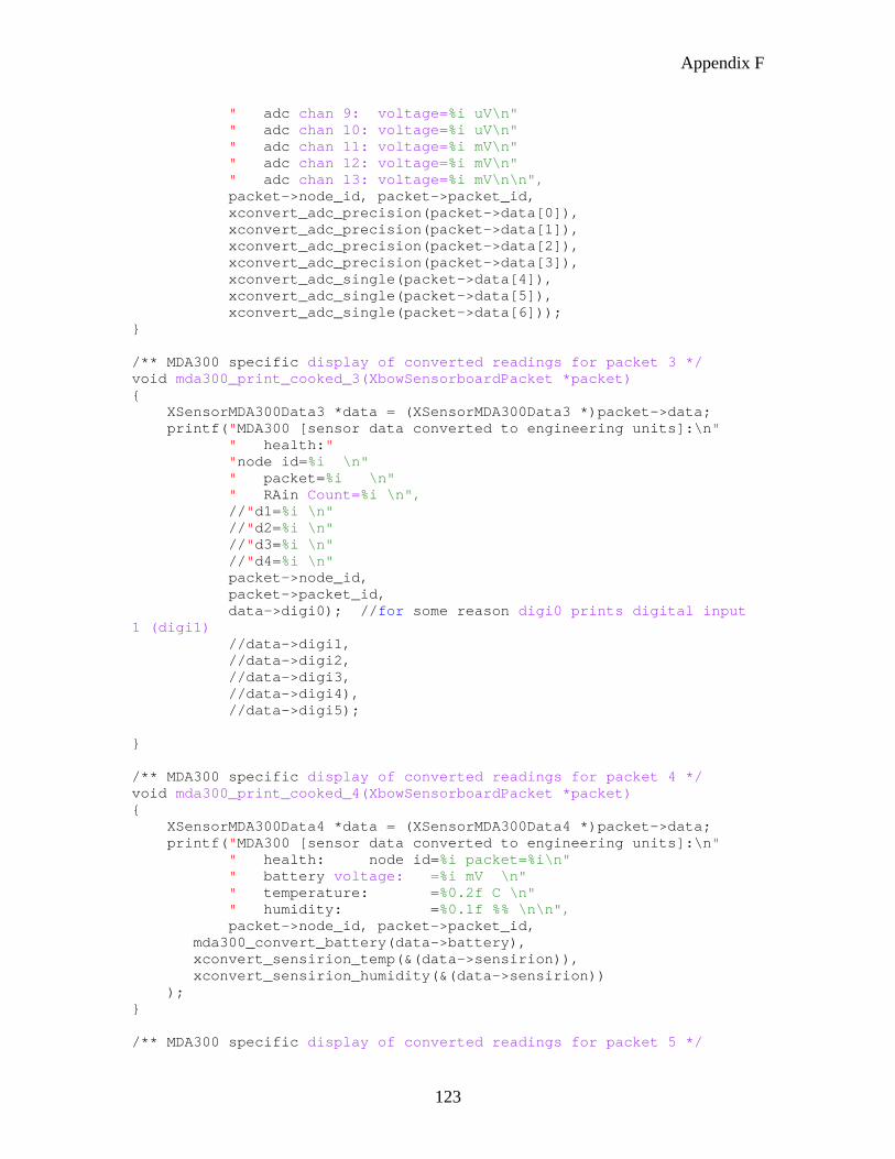
Appendix F
123
" adc chan 9: voltage=%i uV\n" " adc chan 10: voltage=%i uV\n" " adc chan 11: voltage=%i mV\n" " adc chan 12: voltage=%i mV\n" " adc chan 13: voltage=%i mV\n\n", packet->node_id, packet->packet_id, xconvert_adc_precision(packet->data[0]), xconvert_adc_precision(packet->data[1]), xconvert_adc_precision(packet->data[2]), xconvert_adc_precision(packet->data[3]), xconvert_adc_single(packet->data[4]), xconvert_adc_single(packet->data[5]), xconvert_adc_single(packet->data[6])); } /** MDA300 specific display of converted readings for packet 3 */ void mda300_print_cooked_3(XbowSensorboardPacket *packet) { XSensorMDA300Data3 *data = (XSensorMDA300Data3 *)packet->data; printf("MDA300 [sensor data converted to engineering units]:\n" " health:" "node id=%i \n" " packet=%i \n" " RAin Count=%i \n", //"d1=%i \n" //"d2=%i \n" //"d3=%i \n" //"d4=%i \n" packet->node_id, packet->packet_id, data->digi0); //for some reason digi0 prints digital input 1 (digi1) //data->digi1, //data->digi2, //data->digi3, //data->digi4), //data->digi5); } /** MDA300 specific display of converted readings for packet 4 */ void mda300_print_cooked_4(XbowSensorboardPacket *packet) { XSensorMDA300Data4 *data = (XSensorMDA300Data4 *)packet->data; printf("MDA300 [sensor data converted to engineering units]:\n" " health: node id=%i packet=%i\n" " battery voltage: =%i mV \n" " temperature: =%0.2f C \n" " humidity: =%0.1f %% \n\n", packet->node_id, packet->packet_id, mda300_convert_battery(data->battery), xconvert_sensirion_temp(&(data->sensirion)), xconvert_sensirion_humidity(&(data->sensirion)) ); } /** MDA300 specific display of converted readings for packet 5 */
Appendix F
124
void mda300_print_cooked_5(XbowSensorboardPacket *packet) { XSensorMDA300Data5 *data = (XSensorMDA300Data5 *)packet->data; printf("MDA300 [sensor data converted to engineering units]:\n" " health: node id=%i parent=%i battery=%i mV seq_no=%i\n" " adc chan 0: voltage=%i mV\n" " adc chan 1: voltage=%i mV\n" " adc chan 2: voltage=%i mV\n" " temperature: =%0.2f C \n" " humidity: =%0.1f %% \n\n", packet->node_id, packet->parent, mda300_convert_battery(data->battery), data->seq_no, xconvert_adc_single(data->adc0), xconvert_adc_single(data->adc1), xconvert_adc_single(data->adc2), xconvert_sensirion_temp(&(data->sensirion)), xconvert_sensirion_humidity(&(data->sensirion)) ); } /** MDA300 specific display of converted readings from an XSensor packet. */ void mda300_print_cooked(XbowSensorboardPacket *packet) { switch (packet->packet_id) { case 1: mda300_print_cooked_1(packet); break; // Rev B /*case 2: mda300_print_cooked_2(packet); break; */ // case 3: // mda300_print_cooked_3(packet); // break; /* case 4: mda300_print_cooked_4(packet); break; case 5: mda300_print_cooked_5(packet); break; default: printf("MDA300 Error: unknown packet id (%i)\n\n", packet->packet_id); */ // Rev B above we are interested in case 1 only. the rest is commented out } }
Appendix F
125
/** * Logs raw readings to a Postgres database. * * @author Martin Turon * * @version 2004/7/28 mturon Initial revision * */ void mda300_log_raw(XbowSensorboardPacket *packet) { XSensorMDA300Data5 *data = (XSensorMDA300Data5 *)packet->data; if (packet->packet_id != 5) return; char command[512]; char *table = "mda300_results"; sprintf(command, "INSERT into %s " "(result_time,nodeid,parent,epoch,voltage," "humid,humtemp,echo10,echo20,soiltemp)" " values (now(),%u,%u,%u,%u,%u,%u,%u,%u,%u)", table, //timestring, packet->node_id, packet->parent, data->seq_no, data->battery, data->sensirion.humidity, data->sensirion.thermistor, data->adc0, data->adc1, data->adc2 ); xdb_execute(command); } /** * Converts mica2 battery reading from raw ADC data to engineering units. * * @author Martin Turon, Jaidev Prabhu * * We get the reading from MDA300 in 10s of mVolts in ADC counts * * @version 2004/4/6 jdprabhu Changed for MDA300 * */ uint16_t mda300_convert_battery(float x) { // float x = (float)data->battery; uint16_t vdata = (uint16_t) (x * 10); return vdata; } XPacketHandler mda300_packet_handler = { XTYPE_MDA300,
Appendix F
126
"$Id: mda300.c,v 1.18 2004/08/09 16:22:20 jdprabhu Exp $", mda300_print_raw, mda300_print_cooked, mda300_print_raw, mda300_print_cooked, //Rev B see commented out below /*mda300_log_raw*/ }; void mda300_initialize() { xpacket_add_type(&mda300_packet_handler); } F-4: xconvert.c
This file is described in Section 4.3.4. /** * Handles conversion to engineering units for common sensor types. * * @file xconvert.c * @author Martin Turon * modified Jose A. Becerra * @version 2004/8/6 mturon Initial version * * Copyright (c) 2004 Crossbow Technology, Inc. All rights reserved. * * The goals for this module are to provide a general, lucid, and reusable * set of conversion functions for common sensors shared across the diverse * line of Crossbow products. Inputs are usually 16-bit raw ADC readings * and outputs are generally a floating point number in some standard * engineering unit. The standard engineering unit for a few common * measurements follows: * * Temperature: degrees Celsius (C) * Voltage: millvolts (mV) * Pressure: millibar (mbar) * * $Id: xconvert.c,v 1.4 2004/08/11 17:55:47 mturon Exp $ */ #include <math.h> #include "xsensors.h" #include "xconvert.h" /** * Converts mica2 battery reading from raw vref ADC data to engineering units. *
Appendix F
127
* @author Martin Turon * * To compute the battery voltage after measuring the voltage ref: * BV = RV*ADC_FS/data * where: * BV = Battery Voltage * ADC_FS = 1023 * RV = Voltage Reference for mica2 (1.223 volts) * data = data from the adc measurement of channel 1 * BV (volts) = 1252.352/data * BV (mv) = 1252352/data * * Note: * The thermistor resistance to temperature conversion is highly non-linear. * * @version 2004/3/29 mturon Initial revision * @n 2004/8/8 mturon Generalized to xconvert * */ uint16_t xconvert_battery_mica2(uint16_t vref) { float x = (float)vref; uint16_t vdata = (uint16_t) (1252352 / x); return vdata; } /** * Converts battery reading from raw ADC data to engineering units. * * @author Martin Turon, Alan Broad * * To compute the battery voltage after measuring the voltage ref: * BV = RV*ADC_FS/data * where: * BV = Battery Voltage * ADC_FS = 1023 * RV = Voltage Reference (0.6 volts) * data = data from the adc measurement of channel 1 * BV (volts) = 614.4/data * BV (mv) = 614400/data * * Note: * The thermistor resistance to temperature conversion is highly non-linear. * * @return Battery voltage as uint16 in millivolts (mV) * * @version 2004/3/11 mturon Initial revision * @n 2004/8/8 mturon Generalized to xconvert * */ uint16_t xconvert_battery_dot(uint16_t vref) { float x = (float)vref; uint16_t vdata = (uint16_t) (614400 / x); /*613800*/ return vdata;
Appendix F
128
} /** * Converts thermistor reading from raw ADC data to engineering units. * * @author Martin Turon, Alan Broad * * To compute the thermistor resistance after measuring the thermistor voltage: * - Thermistor is a temperature variable resistor * - There is a 10K resistor in series with the thermistor resistor. * - Compute expected adc output from voltage on thermistor as: * ADC= 1023*Rthr/(R1+Rthr) * where R1 = 10K * Rthr = unknown thermistor resistance * Rthr = R1*(ADC_FS-ADC)/ADC * where ADC_FS = 1023 * * Note: * The thermistor resistance to temperature conversion is highly non-linear. * * @return Thermistor resistance as a uint16 in unit (Ohms) * * @version 2004/3/11 mturon Initial revision * */ uint16_t xconvert_thermistor_resistance(uint16_t thermistor) { float adc = (float)thermistor; uint16_t Rthr = 10000 * (1023-adc) / adc; return Rthr; } /** * Converts thermistor reading from raw ADC data to engineering units. * * @author Martin Turon * * @return Temperature reading from thermistor as a float in degrees Celcius * * @version 2004/3/22 mturon Initial revision * @version 2004/4/19 husq * */ float xconvert_thermistor_temperature(uint16_t thermistor) { float temperature, a, b, c, Rthr; a = 0.001307050; b = 0.000214381; c = 0.000000093; Rthr = xconvert_thermistor_resistance(thermistor); temperature = 1 / (a + b * log(Rthr) + c * pow(log(Rthr),3)); temperature -= 273.15; // Convert from Kelvin to Celcius
Appendix F
129
//printf("debug: a=%f b=%f c=%f Rt=%f temp=%f\n",a,b,c,Rt,temperature); return temperature; } /** * Computes the voltage of an adc channel using the reference voltage. * Final formula is designed to minimize fixed point bit shifting * round off errors. * * Convert 12 bit data to mV: * Dynamic range is 0 - 2.5V * voltage = (adc_data * 2500mV) / 4096 * = (adc_data * 625mV) / 1024 * * @author Martin Turon * * @version 2004/3/24 mturon Initial revision * */ uint32_t xconvert_adc_single(uint16_t adc_sing) { uint32_t analog_mV = (625 * (uint32_t)adc_sing) / 1024; return analog_mV; } /** * Calculates the temperature in either *C or *F * depends on what line of code is commented out * in this case output is *F, *C is commented out * *@author Jose A. Becerra * *@version 2006/9/12 */ float xconvert_adc_temp(uint16_t adctemp) { //degrees celcius float temp_eng = (float)(0.5+ (110.2149-1.138253e-1 * adctemp + 7.509040e-5 * adctemp * adctemp -3.188276e-8*adctemp*adctemp*adctemp + 7.069376e-12*adctemp*adctemp*adctemp*adctemp-6.502949e-16*adctemp*adctemp*adctemp*adctemp*adctemp)); //degrees Fahrenheit // float temp_eng = (float) (-0.04077*adctemp + 134.74); return temp_eng; } /** * Computes the voltage of an adc channel using the reference voltage. * Final formula is designed to minimize fixed point bit shifting * round off errors.
Appendix F
130
* * Convert 12 bit data to uV: * Dynamic range is +/- 12.5mV * voltage = 12500 * (adc_data/2048 -1) * = (5*625*data/512) - 12500 * = 5 * ((625*data/512) - 2500) * * * @author Martin Turon * * @version 2004/3/24 mturon Initial revision * */ int32_t xconvert_adc_precision(uint16_t adc_prec) { int32_t analog_uV = 5 * (((625 * (uint32_t)adc_prec)/ 512) - 2500); return analog_uV; } /** * Computes the ADC count of ADXL202E Accelerometer - for X axis reading into * Engineering Unit (mg), per calibration. * * Calibration done for one test sensor - should be repeated for each unit. * * @author Jaidev Prabhu * * @version 2004/3/24 jdprabhu Initial revision * @n 2004/6/17 husq * @n 2004/8/8 mturon Generalized to xconvert * */ float xconvert_accel(uint16_t accel_raw) { uint16_t AccelData; uint16_t calib_neg_1g = 400; uint16_t calib_pos_1g = 500; float scale_factor; float reading; AccelData = accel_raw; scale_factor = ( calib_pos_1g - calib_neg_1g ) / 2; reading = 1.0 - (calib_pos_1g - AccelData) / scale_factor; reading = reading * 1000.0; return reading; } /** * Computes the ADC count of Thermistor into Engineering Unit (degC) *
Appendix F
131
* @author Hu Siquan * * @version 2004/6/25 husq Initial revision * @n 2004/8/8 mturon Generalized to xconvert * */ float xconvert_sensirion_temp(XSensorSensirion *data) { float TempData, fTemp; TempData = (float)data->thermistor; fTemp = -38.4 + 0.0098 * TempData; return fTemp; } /** * Computes the ADC count of Humidity sensor into Engineering Unit (%) * * @author Hu Siquan, Martin Turon * * @version 2004/6/14 husq Initial revision * @n 2004/8/8 mturon Generalized to xconvert * */ float xconvert_sensirion_humidity(XSensorSensirion *data) { float HumData = (float)data->humidity; float fTemp = xconvert_sensirion_temp(data); float fHumidity = -4.0 + 0.0405 * HumData - 0.0000028 * HumData * HumData; fHumidity = (fTemp - 25.0)*(0.01 + 0.00008 * HumData) + fHumidity; return fHumidity; } /** * Computes the pressure ADC count of Intersema MS5534A barometric * pressure/temperature sensor - reading into Engineering Units (mbar) * * @author Hu Siquan * * Intersema MS5534A barometric pressure/temperature sensor * - 6 cal coefficients (C1..C6) are extracted from 4,16 bit,words from sensor * - Temperature measurement: * UT1=8*C5+20224 * dT=data-UT1 * Temp=(degC x10)=200+dT(C6+50)/1024 * - Pressure measurement: * OFF=C2*4 + ((C4-512)*dT)/1024 * SENS=C1+(C3*dT)/1024 + 24576 * X=(SENS*(PressureData-7168))/16384 - OFF * Press(mbar)= X/32+250 *
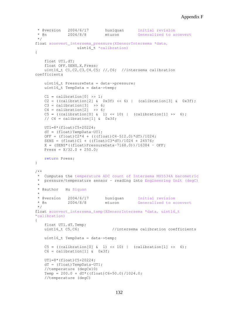
Appendix F
132
* @version 2004/6/17 husiquan Initial revision * @n 2004/8/8 mturon Generalized to xconvert */ float xconvert_intersema_pressure(XSensorIntersema *data, uint16_t *calibration) { float UT1,dT; float OFF,SENS,X,Press; uint16_t C1,C2,C3,C4,C5; //,C6; //intersema calibration coefficients uint16_t PressureData = data->pressure; uint16_t TempData = data->temp; C1 = calibration[0] >> 1; C2 = ((calibration[2] & 0x3f) << 6) | (calibration[3] & 0x3f); C3 = calibration[3] >> 6; C4 = calibration[2] >> 6; C5 = ((calibration[0] & 1) << 10) | (calibration[1] >> 6); // C6 = calibration[1] & 0x3f; UT1=8*(float)C5+20224; dT = (float)TempData-UT1; OFF = (float)C2*4 + (((float)C4-512.0)*dT)/1024; SENS = (float)C1 + ((float)C3*dT)/1024 + 24576; X = (SENS*((float)PressureData-7168.0))/16384 - OFF; Press = X/32.0 + 250.0; return Press; } /** * Computes the temperature ADC count of Intersema MS5534A barometric * pressure/temperature sensor - reading into Engineering Unit (degC) * * @author Hu Siquan * * @version 2004/6/17 husiquan Initial revision * @n 2004/8/8 mturon Generalized to xconvert */ float xconvert_intersema_temp(XSensorIntersema *data, uint16_t *calibration) { float UT1,dT,Temp; uint16_t C5,C6; //intersema calibration coefficients uint16_t TempData = data->temp; C5 = ((calibration[0] & 1) << 10) | (calibration[1] >> 6); C6 = calibration[1] & 0x3f; UT1=8*(float)C5+20224; dT = (float)TempData-UT1; //temperature (degCx10) Temp = 200.0 + dT*((float)C6+50.0)/1024.0; //temperature (degC)

Appendix F
133
Temp /=10.0; return Temp; }
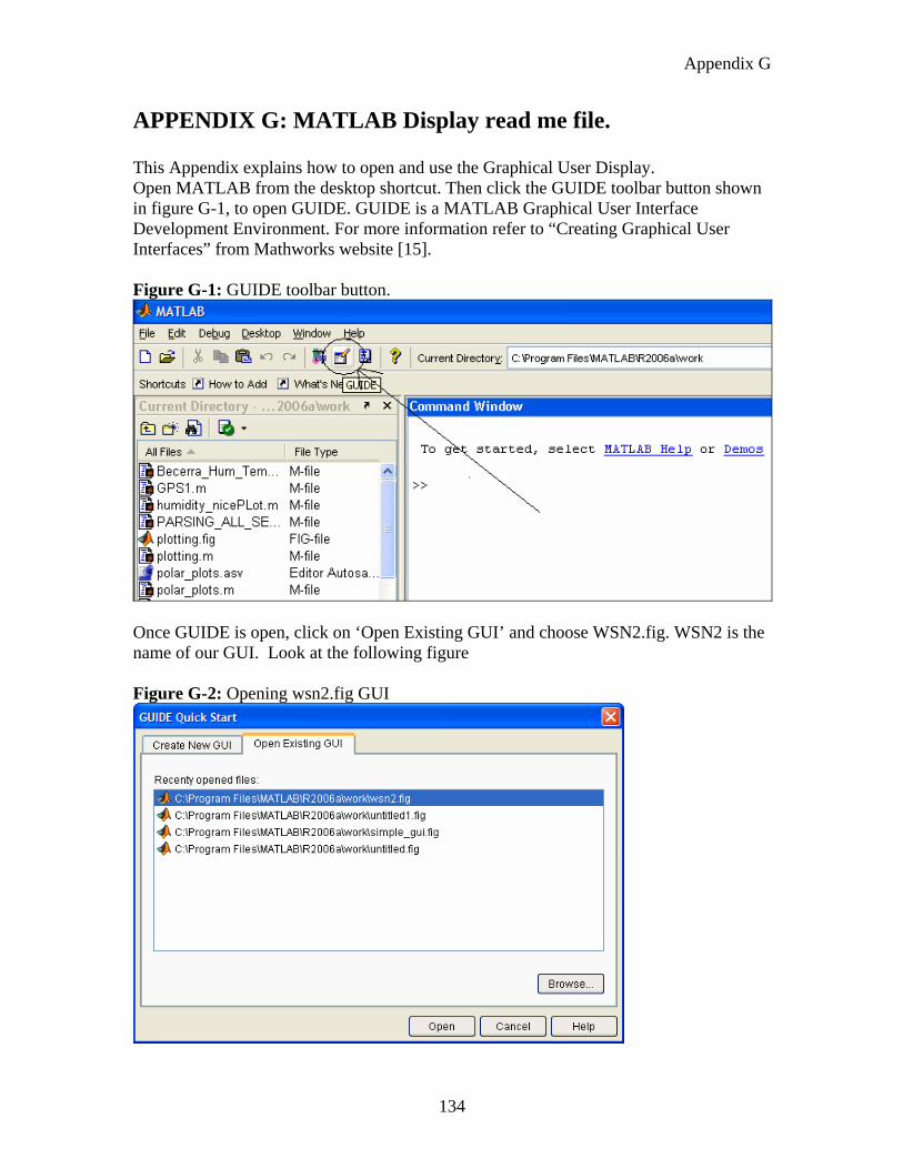
Appendix G
134
APPENDIX G: MATLAB Display read me file. This Appendix explains how to open and use the Graphical User Display. Open MATLAB from the desktop shortcut. Then click the GUIDE toolbar button shown in figure G-1, to open GUIDE. GUIDE is a MATLAB Graphical User Interface Development Environment. For more information refer to “Creating Graphical User Interfaces” from Mathworks website [15]. Figure G-1: GUIDE toolbar button.
Once GUIDE is open, click on ‘Open Existing GUI’ and choose WSN2.fig. WSN2 is the name of our GUI. Look at the following figure Figure G-2: Opening wsn2.fig GUI
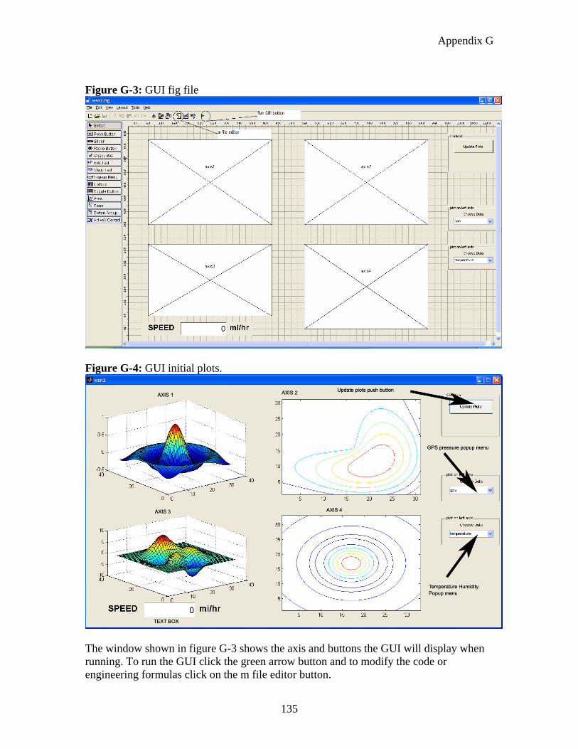
Appendix G
135
Figure G-3: GUI fig file
Figure G-4: GUI initial plots.
The window shown in figure G-3 shows the axis and buttons the GUI will display when running. To run the GUI click the green arrow button and to modify the code or engineering formulas click on the m file editor button.
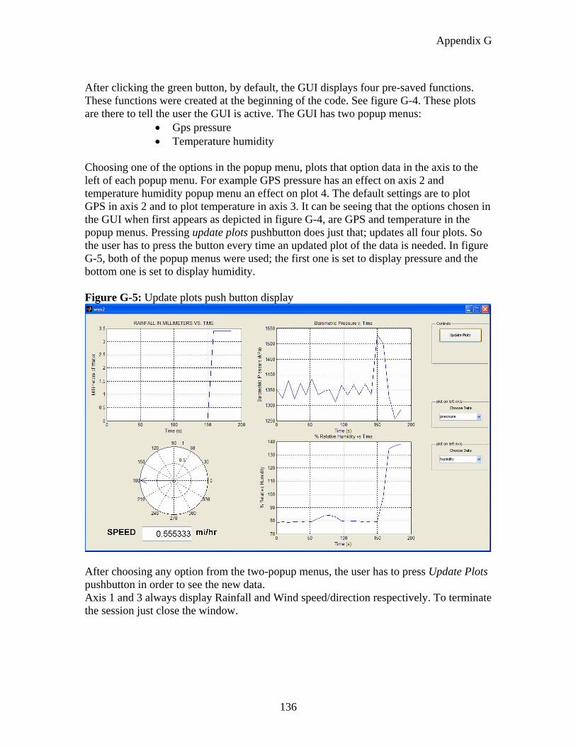
Appendix G
136
After clicking the green button, by default, the GUI displays four pre-saved functions. These functions were created at the beginning of the code. See figure G-4. These plots are there to tell the user the GUI is active. The GUI has two popup menus:
• Gps pressure • Temperature humidity
Choosing one of the options in the popup menu, plots that option data in the axis to the left of each popup menu. For example GPS pressure has an effect on axis 2 and temperature humidity popup menu an effect on plot 4. The default settings are to plot GPS in axis 2 and to plot temperature in axis 3. It can be seeing that the options chosen in the GUI when first appears as depicted in figure G-4, are GPS and temperature in the popup menus. Pressing update plots pushbutton does just that; updates all four plots. So the user has to press the button every time an updated plot of the data is needed. In figure G-5, both of the popup menus were used; the first one is set to display pressure and the bottom one is set to display humidity. Figure G-5: Update plots push button display
After choosing any option from the two-popup menus, the user has to press Update Plots pushbutton in order to see the new data. Axis 1 and 3 always display Rainfall and Wind speed/direction respectively. To terminate the session just close the window.
Appendix H
137
APPENDIX H: MATLAB GUI CODE function varargout = wsn2(varargin) %File Created by Jose A. Becerra % %Last Modified on 12-Sep-2006 22:09:45 %This file opens a cvs file and obtains data to be plotted to 4 displays %please refer to: Becerra, Jose A. "Wireless Sensor Networks demostration %thesis; adding external sensors and a GUI" California Polytechnic State %University, San Luis Obispo EE Masters Thesis Report. September 2006. % %WSN2 M-file for wsn2.fig % WSN2, by itself, creates a new WSN2 or raises the existing % singleton*. % % H = WSN2 returns the handle to a new WSN2 or the handle to % the existing singleton*. % % WSN2('Property','Value',...) creates a new WSN2 using the % given property value pairs. Unrecognized properties are passed % % via % varargin to wsn2_OpeningFcn. This calling syntax produces a % warning when there is an existing singleton*. % % WSN2('CALLBACK') and WSN2('CALLBACK',hObject,...) call the % local function named CALLBACK in WSN2.M with the given input % arguments. % % *See GUI Options on GUIDE's Tools menu. Choose "GUI allows only % one % instance to run (singleton).” % % See also: GUIDE, GUIDATA, GUIHANDLES % Edit the above text to modify the response to help wsn2 % Last Modified by GUIDE v2.5 17-Jun-2006 17:33:45 % Begin initialization code - DO NOT EDIT gui_Singleton = 1; gui_State = struct('gui_Name', mfilename, ... 'gui_Singleton', gui_Singleton, ... 'gui_OpeningFcn', @wsn2_OpeningFcn, ... 'gui_OutputFcn', @wsn2_OutputFcn, ... 'gui_LayoutFcn', [], ... 'gui_Callback', []); if nargin && ischar(varargin{1}) gui_State.gui_Callback = str2func(varargin{1}); end if nargout [varargout{1:nargout}] = gui_mainfcn(gui_State, varargin{:}); else
Appendix H
138
gui_mainfcn(gui_State, varargin{:}); end % End initialization code - DO NOT EDIT % --- Executes just before wsn2 is made visible. function wsn2_OpeningFcn(hObject, eventdata, handles, varargin) % This function has no output args, see OutputFcn. % hObject handle to figure % eventdata reserved - to be defined in a future version of MATLAB % handles structure with handles and user data (see GUIDATA) % varargin unrecognized PropertyName/PropertyValue pairs from the % command line (see VARARGIN) %Create the data to plot %Creates Any data so when the GUI first appears displays something %until user clicks the update button. handles.peaks=peaks(35); handles.membrane=membrane; [x,y] = meshgrid(-8:.5:8); r = sqrt(x.^2+y.^2) + eps; sinc = sin(r)./r; handles.sinc = sinc; %initial plots that appear when GUI is Run axes(handles.axis1); %sets the axis to which we can plot surf(handles.sinc); axes(handles.axis2); %sets the axis to which we can plot contour(handles.membrane); axes(handles.axis3); %sets the axis to which we can plot surf(handles.peaks); axes(handles.axis4); %sets the axis to which we can plot contour(handles.sinc); %**************************************************************** handles.run_flag=0; %initialize flags handles.gps_plot_flag = 1; handles.pressure_plot_flag = 0; handles.humidity_plot_flag = 0; handles.temperature_plot_flag = 1; % Choose default command line output for wsn2 handles.output = hObject; % Update handles structure guidata(hObject, handles); % UIWAIT makes wsn2 wait for user response (see UIRESUME) % uiwait(handles.figure1); % --- Outputs from this function are returned to the command line. function varargout = wsn2_OutputFcn(hObject, eventdata, handles)
Appendix H
139
% varargout cell array for returning output args (see VARARGOUT); % hObject handle to figure % eventdata reserved - to be defined in a future version of MATLAB % handles structure with handles and user data (see GUIDATA) % Get default command line output from handles structure varargout{1} = handles.output; % --- Executes on button press in update_pushbutton. function update_pushbutton_Callback(hObject, eventdata, handles) % hObject handle to update_pushbutton (see GCBO) % eventdata reserved - to be defined in a future version of MATLAB % handles structure with handles and user data (see GUIDATA) x=0; handles.data=csvread('C:\tinyos\cygwin\opt\tinyos-1.x\contrib\xbow\tools\src\xlisten\all_sensors.csv',4,0); %row=4 column=0; %handles.data=csvread('C:\tinyos\cygwin\opt\tinyos-1.x\contrib\xbow\tools\src\xlisten\temp.csv',4,0); %row=4 column=0; board_id=handles.data(:,1); Max1=size(board_id); %Initialize Gps data if no data is recorded m_gps=ones(1,14); %handles.current_data = handles.ieplot; j=1; k=1; for n =1:Max1, if (board_id(n) == 81) %write that row of data to a matrix called sensors m_sensors(j,:)=handles.data(n,:); j=j+1; else m_gps(k,:)=handles.data(n,:); k=k+1; end %end if else %search for GPS data end %for loop %assign main sensor readings to handles structure handles.time=m_sensors(:,2) time=m_sensors(:,2); handles.counter=m_sensors(:,7); handles.direction=m_sensors(:,8); handles.pres=m_sensors(:,9); handles.humidity=m_sensors(:,10); handles.rain_gauge=m_sensors(:,11); handles.temperature=m_sensors(:,12); %assign GPS data to plot handles.gps=m_gps; handles.latitude=m_gps(:,5); handles.longitude=m_gps(:,6);
Appendix H
140
%handles.current_data = handles.direction; %update handles structure guidata(hObject, handles); %****************************************************************** axes(handles.axis1); %sets the axis to which we can plot plot(handles.time,handles.rain_gauge*0.2); %conversion formula grid %plot command xlabel('Time (s)') ylabel('Millimeters of Water') Title('RAINFALL IN MILLIMETERS VS. TIME') %****************************************************************** axes(handles.axis2); %sets the axis to which we can plot if handles.gps_plot_flag == 1 plot(handles.longitude,handles.latitude); %this will depend on xlabel('Longitude') %popup menu ylabel('Latitude') Title('GPS Location') else handles.pressure = 0.02222*2*handles.pres +10.556; guidata(hObject, handles); plot(handles.time,handles.pressure); grid xlabel('Time (s)') ylabel('Barometric Pressure (kPa)') Title('Barometric Pressure vs. Time') end %****************************************************************** axes(handles.axis3); % plot(handles.time,handles.direction); % xlabel('Time (s)') ylabel('Wind Direction Degrees') Title('WIND DIRECTION AND SPEED') %calculation of wind speed time = handles.time; rev = handles.counter; last=size(time); for n =2:last(1) time_delta(n)=(time(n) - time(n-1)); %time between readings end for n=2:last %speed formula below; see section 5.3.2 speed(n)=rev(n)* (4 * 3.1416)/(time_delta(n)); %in ft/sec handles.speed_mi_hr(n)=speed(n)/17.6; %mi/hr end %save to handles structure guidata(hObject, handles); %write speed as a number in a text box
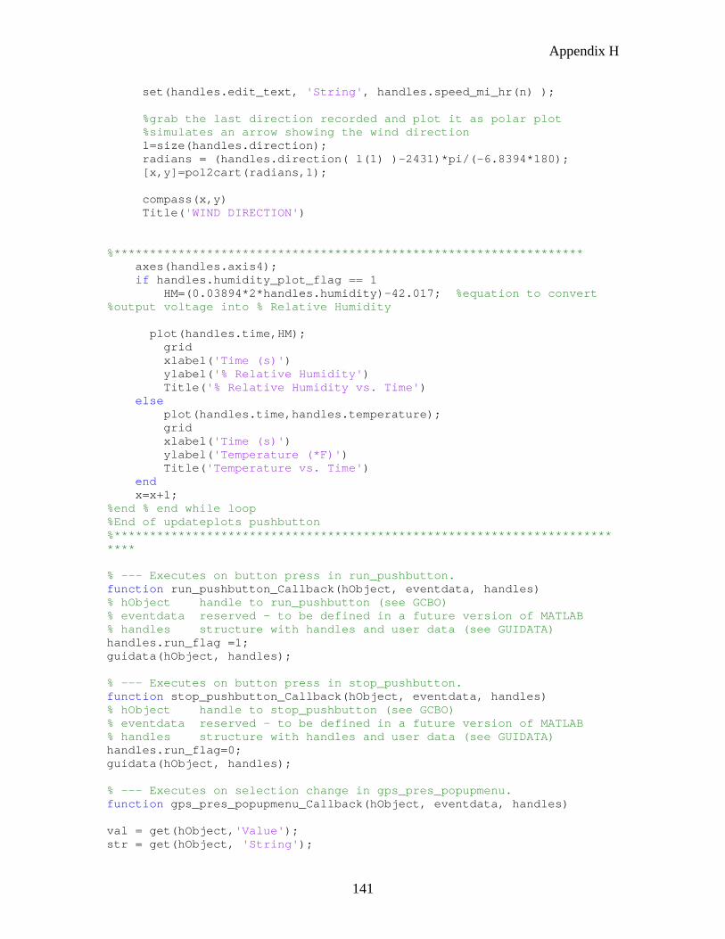
Appendix H
141
set(handles.edit_text, 'String', handles.speed_mi_hr(n) ); %grab the last direction recorded and plot it as polar plot %simulates an arrow showing the wind direction l=size(handles.direction); radians = (handles.direction( l(1) )-2431)*pi/(-6.8394*180); [x,y]=pol2cart(radians,1); compass(x,y) Title('WIND DIRECTION') %****************************************************************** axes(handles.axis4); if handles.humidity_plot_flag == 1 HM=(0.03894*2*handles.humidity)-42.017; %equation to convert %output voltage into % Relative Humidity
plot(handles.time,HM); grid xlabel('Time (s)') ylabel('% Relative Humidity') Title('% Relative Humidity vs. Time') else plot(handles.time,handles.temperature); grid xlabel('Time (s)') ylabel('Temperature (*F)') Title('Temperature vs. Time') end x=x+1; %end % end while loop %End of updateplots pushbutton %************************************************************************** % --- Executes on button press in run_pushbutton. function run_pushbutton_Callback(hObject, eventdata, handles) % hObject handle to run_pushbutton (see GCBO) % eventdata reserved - to be defined in a future version of MATLAB % handles structure with handles and user data (see GUIDATA) handles.run_flag =1; guidata(hObject, handles); % --- Executes on button press in stop_pushbutton. function stop_pushbutton_Callback(hObject, eventdata, handles) % hObject handle to stop_pushbutton (see GCBO) % eventdata reserved - to be defined in a future version of MATLAB % handles structure with handles and user data (see GUIDATA) handles.run_flag=0; guidata(hObject, handles); % --- Executes on selection change in gps_pres_popupmenu. function gps_pres_popupmenu_Callback(hObject, eventdata, handles) val = get(hObject,'Value'); str = get(hObject, 'String');
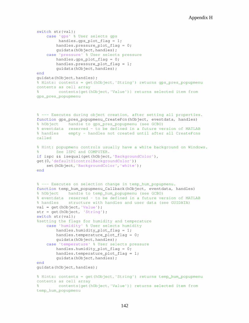
Appendix H
142
switch str{val}; case 'gps' % User selects gps handles.gps_plot_flag = 1; handles.pressure_plot_flag = 0; guidata(hObject,handles); case 'pressure' % User selects pressure handles.gps_plot_flag = 0; handles.pressure_plot_flag = 1; guidata(hObject,handles); end guidata(hObject,handles); % Hints: contents = get(hObject,'String') returns gps_pres_popupmenu contents as cell array % contents{get(hObject,'Value')} returns selected item from gps_pres_popupmenu % --- Executes during object creation, after setting all properties. function gps_pres_popupmenu_CreateFcn(hObject, eventdata, handles) % hObject handle to gps_pres_popupmenu (see GCBO) % eventdata reserved - to be defined in a future version of MATLAB % handles empty - handles not created until after all CreateFcns called % Hint: popupmenu controls usually have a white background on Windows. % See ISPC and COMPUTER. if ispc && isequal(get(hObject,'BackgroundColor'), get(0,'defaultUicontrolBackgroundColor')) set(hObject,'BackgroundColor','white'); end % --- Executes on selection change in temp_hum_popupmenu. function temp_hum_popupmenu_Callback(hObject, eventdata, handles) % hObject handle to temp_hum_popupmenu (see GCBO) % eventdata reserved - to be defined in a future version of MATLAB % handles structure with handles and user data (see GUIDATA) val = get(hObject,'Value'); str = get(hObject, 'String'); switch str{val}; %setting the flags for humidity and temperature case 'humidity' % User selects humidity handles.humidity_plot_flag = 1; handles.temperature_plot_flag = 0; guidata(hObject,handles); case 'temperature' % User selects pressure handles.humidity_plot_flag = 0; handles.temperature_plot_flag = 1; guidata(hObject,handles); end guidata(hObject,handles); % Hints: contents = get(hObject,'String') returns temp_hum_popupmenu contents as cell array % contents{get(hObject,'Value')} returns selected item from temp_hum_popupmenu
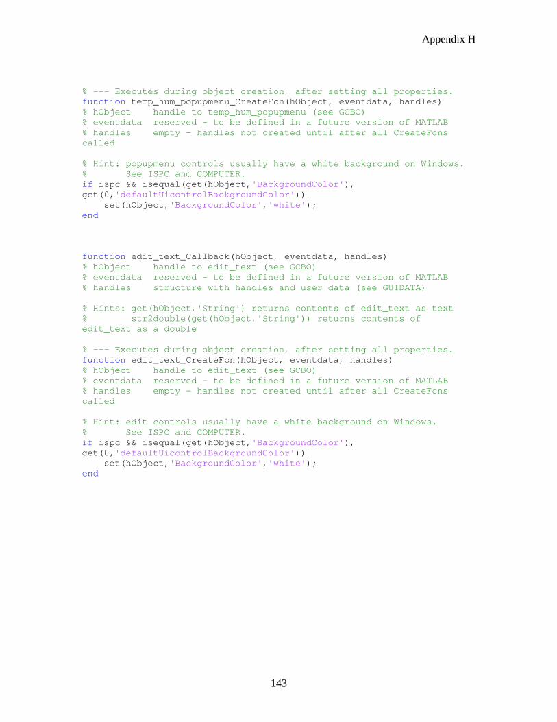
Appendix H
143
% --- Executes during object creation, after setting all properties. function temp_hum_popupmenu_CreateFcn(hObject, eventdata, handles) % hObject handle to temp_hum_popupmenu (see GCBO) % eventdata reserved - to be defined in a future version of MATLAB % handles empty - handles not created until after all CreateFcns called % Hint: popupmenu controls usually have a white background on Windows. % See ISPC and COMPUTER. if ispc && isequal(get(hObject,'BackgroundColor'), get(0,'defaultUicontrolBackgroundColor')) set(hObject,'BackgroundColor','white'); end function edit_text_Callback(hObject, eventdata, handles) % hObject handle to edit_text (see GCBO) % eventdata reserved - to be defined in a future version of MATLAB % handles structure with handles and user data (see GUIDATA) % Hints: get(hObject,'String') returns contents of edit_text as text % str2double(get(hObject,'String')) returns contents of edit_text as a double % --- Executes during object creation, after setting all properties. function edit_text_CreateFcn(hObject, eventdata, handles) % hObject handle to edit_text (see GCBO) % eventdata reserved - to be defined in a future version of MATLAB % handles empty - handles not created until after all CreateFcns called % Hint: edit controls usually have a white background on Windows. % See ISPC and COMPUTER. if ispc && isequal(get(hObject,'BackgroundColor'), get(0,'defaultUicontrolBackgroundColor')) set(hObject,'BackgroundColor','white'); end
Appendix I
144
APPENDIX I: Source Files Read me. The TinyOS source files that were used/modified in this project are included in the accompanying compact disc. It also includes: this project report, the MATLAB files needed to run the graphical user interface, and sample sensor and GPS data (.csv files). The following files are included in the folder called src:
• Xlisten.c
• Mda300.c
• XSensorMDA300M.nc
• Xconvert.c
• Sample .csv files
The following files are included in the folder called Matlab_Work:
• WSN2.m
• WSN2.fig
• WSN2.asp
Save the src folder in the following directory:
C:\tinyos\cygwin\opt\tinyos-1.x\contrib\xbow\tools\
Save the Matlab_Work contents in the MATLAB work directory.
C:\Program Files\MATLAB\R2006a\work
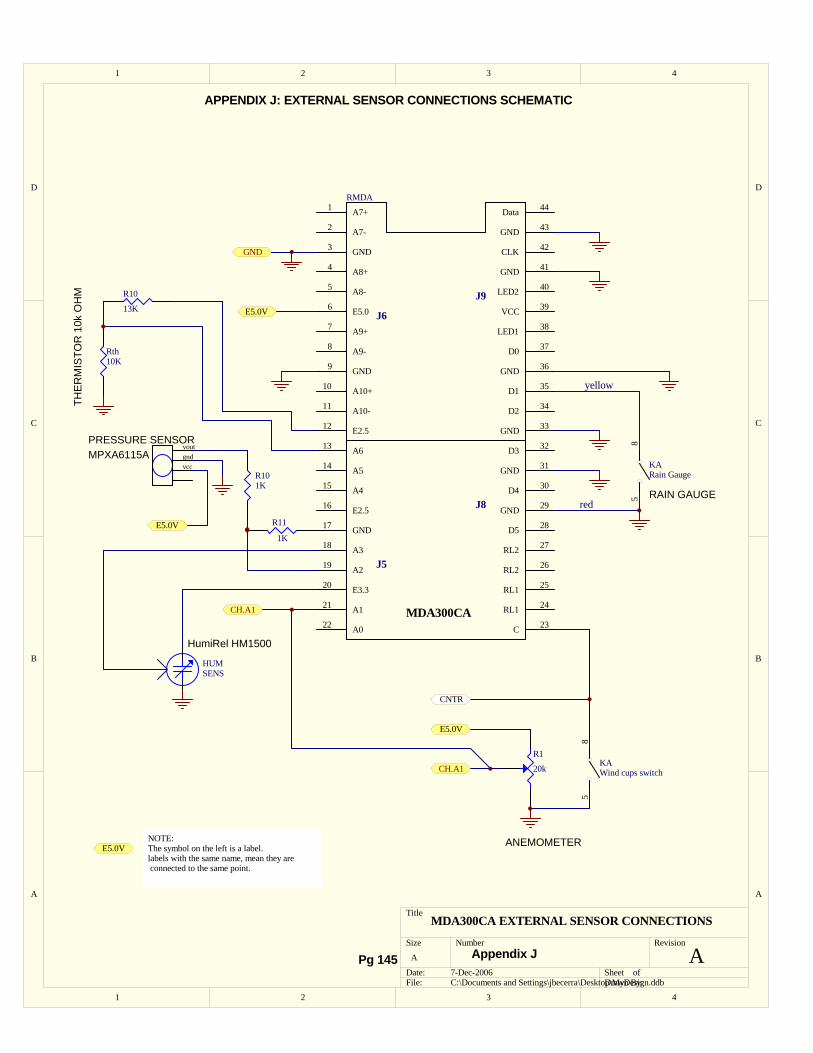
1 2 3 4
A
B
C
D
4321
D
C
B
A
Title
Number RevisionSize
A
Date: 7-Dec-2006 Sheet of File: C:\Documents and Settings\jbecerra\Desktop\MyDesign.ddbDrawn By:
R1
20k
85
KAWind cups switch
CNTR
A7+1
A7-2
GND3
A8+4
A8-5
E5.06
A9+7
A9-8
GND9
A10+10
A10-11
E2.512
A613
A514
A415
E2.516
GND17
A318
A219
E3.320
A121
A022 C 23
RL1 24
RL1 25
RL2 26
RL2 27
D5 28
GND 29
D4 30
GND 31
D3 32
GND 33
D2 34
D1 35
GND 36
D0 37
LED1 38
VCC 39
LED2 40
GND 41
CLK 42
GND 43
Data 44
J6
J5
J8
J9
MDA300CA
RMDA
HUMSENS
E5.0V
E5.0V
CH.A1
CH.A1
GND
85
KARain Gauge
red
yellow
R101K
R11
1KE5.0V
vcc
voutgnd
MDA300CA EXTERNAL SENSOR CONNECTIONS
A
E5.0VNOTE:The symbol on the left is a label.labels with the same name, mean they are connected to the same point.
MPXA6115A
HumiRel HM1500
ANEMOMETER
RAIN GAUGE
PRESSURE SENSOR
R10
13K
THE
RM
ISTO
R 1
0k O
HM
Rth10K
Appendix J
APPENDIX J: EXTERNAL SENSOR CONNECTIONS SCHEMATIC
Pg 145
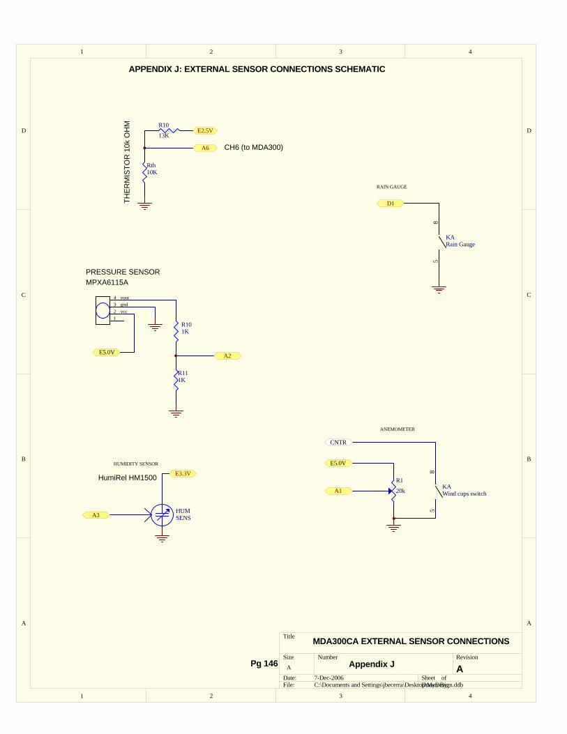
1 2 3 4
A
B
C
D
4321
D
C
B
A
Title
Number RevisionSize
A
Date: 7-Dec-2006 Sheet of File: C:\Documents and Settings\jbecerra\Desktop\MyDesign.ddbDrawn By:
R1
20k
85
KAWind cups switch
CNTR
HUMSENS
E5.0V
A1
85
KARain Gauge
R101K
R111K
E5.0V
vcc
voutgnd
A2
E3.3V
A3
D1
HUMIDITY SENSOR
ANEMOMETER
RAIN GAUGE
R10
13KTH
ER
MIS
TOR
10k
OH
ME2.5V
A6 CH6 (to MDA300)
MDA300CA EXTERNAL SENSOR CONNECTIONS
A
MPXA6115A
HumiRel HM1500
PRESSURE SENSOR
1234
Rth10K
Appendix JPg 146
APPENDIX J: EXTERNAL SENSOR CONNECTIONS SCHEMATIC