Structural Algorithms in RODON

With a prototype implementation in Java

Master’s thesis performed at the Vehicular Systems division, department of Electrical Engineering at

Linköping University

by

Oskar Särnholm

Reg nr: LiTH-ISY-EX--07/3925--SE

2007

ii

iii

Structural Algorithms in RODON

With a prototype implementation in Java

A masters thesis performed in Linköping Institute of Technology

by

Oskar Särnholm

LiTH-ISY-EX--07/3925--SE

Academic supervisor: Dr Mattias Krysander Industrial supervisor: Dr Peter Bunus Examiner: Dr Erik Frisk February 14, 2007

iv

v

Presentationsdatum Mars 2, 2007 Publiceringsdatum (elektronisk version)

Institution och avdelning Institutionen för systemteknik

Department of Electrical Engineering

URL för elektronisk version http://www.ep.liu.se

Publikationens titel Structural Algorithms in RODON with a prototype implementation in Java Författare Oskar Särnholm

Sammanfattning As machines are increasingly used to fulfill even more needs of mankind, the dependence upon those machines increase. To prevent catastrophic failure and to facilitate maintenance a diagnostic system can be used. A diagnostic system supervises the system and can alarm the operator when a fault has occurred, and possibly determine what the cause may be. One architecture of a diagnostic system is a number of tests run by an on-board computer checking certain combinations of sensor values and control signals chosen in advance. To design these tests is a difficult task, which leads to the desire to automate the test construction. A part of this task can be performed using structural methods. In this thesis model based diagnosis is considered. This means that a formal mathematical model is used. The models typically consist of a number of equations describing the behavior of the system. In structural methods it is only considered if a variable exists in an equation or not. The goal of this master thesis project has been to apply structural methods to RODON models. RODON is a software diagnostics tool brought to market by Sörman Information & Media, which can perform various diagnostic-related tasks based on a single model. This model is defined in an object oriented fashion using a Modelica-like language called Rodelica. A prototype implementation of a structural algorithm plug-in has been developed and integrated into RODON. An additional part of the project has been to investigate further possible uses of structural algorithms in RODON, apart from diagnostic test construction. This has been performed as a series of interviews with Sörman and university employees. The work performed in this thesis has shown that it is possible to apply structural methods to RODON models. It has also shown that even a prototype implementation can handle quite large systems. Some problems have been found as well, most notably in extracting a structural model from a RODON model. A consequence is that the developed structural plug-in only works for a subset of RODON models. It might be possible to deal with these problems if more time would be spent on the task. Finally, the interview survey revealed other possible uses of structural methods in RODON, including optimal sensor placement analysis and isolability and detectability analysis.

Nyckelord Model-based diagnosis, structural methods, Rodon

Språk Svenska x Annat (ange nedan) Engelska Antal sidor 57

Typ av publikation Licentiatavhandling x Examensarbete C-uppsats D-uppsats Rapport Annat (ange nedan)

ISBN (licentiatavhandling)

ISRN

Serietitel (licentiatavhandling)

Serienummer/ISSN (licentiatavhandling)

vi

vii

Abstract As machines are increasingly used to fulfill even more needs of mankind, the dependence upon those machines increase. To prevent catastrophic failure and to facilitate maintenance a diagnostic system can be used. A diagnostic system supervises the system and can alarm the operator when a fault has occurred, and possibly determine what the cause may be. One architecture of a diagnostic system is a number of tests run by an on-board computer checking certain combinations of sensor values and control signals chosen in advance. To design these tests is a difficult task, which leads to the desire to automate the test construction. A part of this task can be performed using structural methods. In this thesis model based diagnosis is considered. This means that a formal mathematical model is used. The models typically consist of a number of equations describing the behavior of the system. In structural methods it is only considered if a variable exists in an equation or not. The goal of this master thesis project has been to apply structural methods to RODON models. RODON is a software diagnostics tool brought to market by Sörman Information & Media, which can perform various diagnostic-related tasks based on a single model. This model is defined in an object oriented fashion using a Modelica-like language called Rodelica. A prototype implementation of a structural algorithm plug-in has been developed and integrated into RODON. An additional part of the project has been to investigate further possible uses of structural algorithms in RODON, apart from diagnostic test construction. This has been performed as a series of interviews with Sörman and university employees. The work performed in this thesis has shown that it is possible to apply structural methods to RODON models. It has also shown that even a prototype implementation can handle quite large systems. Some problems have been found as well, most notably in extracting a structural model from a RODON model. A consequence is that the developed structural plug-in only works for a subset of RODON models. It might be possible to deal with these problems if more time would be spent on the task. Finally, the interview survey revealed other possible uses of structural methods in RODON, including optimal sensor placement analysis and isolability and detectability analysis.

viii

ix

Acknowledgements I would like to express my gratitude to a number of people: My academic supervisor Mattias Krysander. He has always been patient with me taking time to discuss and explain many issues, and he has been of great help during the whole project. My examiner Erik Frisk, and the rest of the people at Vehicular systems department for interesting discussions during breaks and lunches. My industrial supervisor Peter Bunus at Sörman Information & Media for making this thesis possible, and for contributing greatly, always taking time to answer my questions. Henrik Johansson for helping me out with programming issues, Frank Seifart for helping me with RODON issues, and the rest of the Sörman crew, in Linköping as well as in Heidenheim, for nice discussion during breaks and lunches. Finally my opponent Rickard Hyllenstam for giving comments on the manuscript during the working process, and last but not least to Daniel Andersson and Patrik Sköld for interesting discussions on diagnostics and RODON.

x

xi

Contents 1 Introduction ....................................................................................................................1

1.1 Background.............................................................................................................1 1.2 Problem Formulation...............................................................................................2 1.3 Objectives ...............................................................................................................2 1.4 Thesis Outline .........................................................................................................2

2 Diagnostics Theory .........................................................................................................3 2.1 Terminology and definitions....................................................................................3 2.2 Diagnostic Systems .................................................................................................4 2.3 Different views on diagnostics ................................................................................5

3 Structural Methods..........................................................................................................7 3.1 Structural models ....................................................................................................7

3.1.1 Matrix form.....................................................................................................7 3.1.2 Graph form......................................................................................................7

3.2 Properties of graphs.................................................................................................8 3.3 Finding the overdetermined part..............................................................................9 3.4 Properties of structural models ..............................................................................10 3.5 Use of MSO sets in diagnostic system design..........................................................10 3.6 Structural algorithms.............................................................................................11

3.6.1 The basic algorithm .......................................................................................11 3.6.2 The improved algorithm ................................................................................13

4 RODON ..........................................................................................................................17 4.1 Rodelica................................................................................................................17 4.2 Simulation in RODON .............................................................................................18 4.3 Model characteristics.............................................................................................18

4.3.1 The OR Clause ..............................................................................................18 4.4 Model classes........................................................................................................19 4.5 Modelling in RODON..............................................................................................19

5 Structural algorithm prototypes in rodon .......................................................................21 5.1 Extracting equations and variables ........................................................................21

5.1.1 Challenges in extracting variables..................................................................21 5.1.2 Challenges in extracting equations.................................................................22 5.1.3 Actual implementation ..................................................................................22

5.2 Implementation of structural algorithms ................................................................23 5.3 Application to an example.....................................................................................24 5.4 Limitations of the prototype ..................................................................................27 5.5 Modeling guidelines..............................................................................................27 5.6 Empirical time complexity analysis .......................................................................27

5.6.1 Dependence on the number of equations........................................................28 5.6.2 Dependence on redundancy ...........................................................................28 5.6.3 Conclusions...................................................................................................29

6 Other uses of structural algorithms in RODON ................................................................31 6.1 Interview results from employees at Sörman .........................................................31 6.2 Interview results from researchers at Vehicular Systems Department ....................31 6.3 Summary and comments .......................................................................................33

7 Discussion and Future Work .........................................................................................35 8 Conclusions ..................................................................................................................37 9 References ....................................................................................................................39

xii

1

1 INTRODUCTION This chapter introduces the reader to the background of the thesis and the field of diagnosis. It also describes the problem that is studied, and the reason why it is of interest. Finally, it features an outline of the thesis.

1.1 Background

As technology is being developed, it is possible to create systems with increasing capabilities that can satisfy the needs of mankind better every day. However this also means that the complexity of technical systems increases, as does our dependence upon their correct operation. Failure of technical systems around us can in many cases lead to environmental, personal, and economic damages. Examples of this are not hard to find, the control system of a nuclear power plant, the landing gear system of a passenger aircraft, and the production facilities of a modern company are some. Thus arise the need of means to prevent essential systems from failing. This can be done using a device, which can detect the presence of a fault before it leads to performance degradation or catastrophic failure of the whole system. Such a system is called a diagnostic system. A diagnostic system can also be able to isolate the faulty component in a larger system. This can help service personal performing quicker maintenance and thus the return to normal operation of the system. Early means to diagnose a system was manual inspection. The operator would use her senses, such as smelling, looking for anomalous behavior, listening for strange noises and trying to sense abnormal vibrations. With the introduction of computers and electronics, diagnosis can be performed by checking that certain sensor values are within normal operating ranges. In this thesis, model-based diagnosis is considered. In model-based diagnosis, a mathematical model of the system is used. For example the model can be fed with the same input as the real system. The output of the real system and of the model can then be inspected, and from that, conclusions can be drawn about the real system. Model-based diagnosis has a number of advantages compared to traditional diagnosis. For example it is sensible to smaller faults, reacts faster and gives better possibilities for fault isolation. This master’s thesis has been performed at Sörman information & media (henceforth called “Sörman”) and the Vehicular Systems department, a part of Electrical Engineering at Linköping University (henceforth called “Vehicular Systems department”). Sörman is described on their corporate web page as “…a leading technology provider of Product

Lifecycle Management (PLM) information solutions and services for advanced products and

systems.” (Sörman, 2006) At the Vehicular division, research is conducted in the fields of vehicular control systems, diagnosis and function supervision (Vehicular Systems Department, 2006). Sörman develops and markets a software product for diagnosis called RODON. In RODON, many different types of diagnostic-related tasks can be performed once a model of the systems is constructed. Henceforth, such a system model will be called a “RODON model”. Typically, RODON is used for offline diagnosis. That is, RODON is normally not connected to the diagnosed system during operation. Instead, it is typically used when a fault in the systems is already detected. For example it can be used to calculate the root cause of a symptom in the electrical system of a car. At Vehicular Systems Department, a diagnostic system is typically considered to be online, that is hooked up to, and constantly diagnosing the system.

2

1.2 Problem Formulation

A common architecture for performing online diagnostics is to use a diagnostic system constantly running a number of tests. In each test, some calculations are made on some observations from the system. The observations can for example be control signals and sensor signals. Each test is designed to react to some faults and should raise an alarm if any of these faults are present. An important part of designing a diagnostic system is to decide which such tests the diagnosis system should be composed of. There are a number of requirements on these tests, and finding a suitable set of test that fulfils all requirements is a complicated task. Today, a suitable test set is typically found manually. This is a time-consuming and error-prone assignment, and small changes in the system design can lead to the need to redesign the whole diagnostic system. It would be a substantial gain if this task could be handled automatically. A mathematical model of the system offers a possibility to accomplish this. By applying suitable methods to the model, appropriate fault tests can be found. More explicit, this means finding all subsets of the total equation system that can be used to design fault tests. To find all of these usable subsets automatically for large systems is a difficult task. Previous attempts to perform this task automatically have been too demanding on computational resources to be an alternative for large systems. At Vehicular Systems Department, methods for finding all subsets of the mathematical model usable to construct fault tests have been developed. These methods are structural. That means that they only take into account whether a certain variable is present in a certain equation or not. The model in RODON can already be used for many different tasks. Adding the possibility to apply structural methods would further extend the usefulness of constructing a RODON model. Furthermore, designing an online diagnostic system typically involves 1) selection of which subsets of the model that should be used to construct diagnostic tests, 2) construction of these tests and 3) validate the test against measurements from the real system. Selecting only the subsets needed in 1 will save time in step 3, since no time will be spent validating unnecessary tests. (Krysander, 2006)

1.3 Objectives

The main objective of this thesis is to apply structural methods to RODON models. More specifically, this means extracting the equations and variables describing the RODON model and applying the algorithms developed at Vehicular Systems Department to extract the subsets of equations mentioned above. A prototype implementation has been developed and integrated as a module into RODON. Today, RODON does not include functionality to extract these subsets of equations. Another objective of this thesis is to investigate other uses of structural methods than test construction in RODON.

1.4 Thesis Outline

The thesis is structured as follows: In chapter 2, the theoretic foundation of diagnostics is laid. Chapter 3 contains a series of definitions leading to being able to define exactly what output is wanted from structural algorithms. It also features the algorithms themselves. In Chapter 4, some aspects of the software tool RODON is presented. These aspects are used in Chapter 5 where the actual prototype implementation is presented. In Chapter 6 the results of the interviews on further uses of structural algorithms in RODON is presented, and finally Chapter 7 and 8 contains discussion and conclusions respectively.

3

2 DIAGNOSTICS THEORY This chapter introduces the reader to the field of diagnostics. An architecture for on-line diagnostic systems is presented. Finally, an outlook to other approaches to diagnostics is offered.

2.1 Terminology and definitions

The following terminology for diagnostic systems was agreed upon by the Technical Committee on SAFEPROCESS of the International Federation of Automatic Control (IFAC) as presented in Blanke et al (2003). The terms will be used with these meanings throughout the thesis. Fault Unpermitted deviation of at least one characteristic property or parameter

of the system from its acceptable / usual / standard condition. Failure Permanent interruption of a systems ability to perform a required function

under specified operating conditions. Residual Fault information carrying signals, based on deviation between

measurements and model computations. Fault detection Determination of faults present in a system and time of detection. Fault isolation Determination of kind, location and time of detection of a fault. Follows

fault detection. Fault diagnosis Determination of kind, size, location and time of occurrence of a fault.

Fault diagnosis includes fault detection, isolation and estimation. In Figure 2.1, a schematic view of an on-line diagnostic system is presented.

Figure 2.1 - Diagnosis of a continuous system

System u y

- +

Evaluate Residual

Faults, Disturbances

r

Diagnostic system

ŷ

Diagnostic Statement

Model

4

The system is controlled by the control signal or actuator u and generates an output y. Faults

and disturbances affect the system. The part surrounded by a dashed line is the diagnostic system. The diagnostic system takes the inputs and outputs of the real system as inputs, and delivers a diagnostic statement as output. Inside the diagnostic system, a model of the real fault free system is fed with the same actuator signal as the real system and estimates ŷ. The difference between the system output y and the model output ŷ is called a residual r. If r = 0 no conclusion is drawn. If r ≠ 0 one concludes that a fault is present in the system. In the real world, r will typically not be equal to 0 due to noise in the signals. Instead it is checked whether |r| < some tolerance.

2.2 Diagnostic Systems

The goal of a diagnostic system is to detect and preferably isolate faults in a system. As described in Section 1.1, different kind of diagnostic systems are possible. In this thesis we will treat model-based diagnostics. As mentioned above, an explicit mathematical model of the system is used. This means that we have a set of equations describing the behavior of the system. To be able to perform diagnosis we need analytical redundancy in the model. That is, we need more than one way to calculate a certain variable. If we for example have two ways to calculate the variable x, we can compare the two results. If both ways give the same value on x, it seems ok. If we get different results, we may have a problem. In Figure 2.1 we have two ways of determining the output of the system: By measuring the actual system output and by calculating what the output should be using the model and the input to the system. Analytical redundancy is formally defined as follows:

Definition 2.1 (Analytical redundancy): There exists analytical redundancy if there exists two or more

ways to determine a variable where one of the ways use a mathematical model.

A system is assumed to be working in exactly one of several predefined behavioral modes. Here, the set of all possible behavioral modes is denoted B, and includes the no-fault mode, some fault modes and the unknown-fault mode. A set of behavioral modes for a system consisting of a light bulb and a switch can for example be B = {no fault, bulb broken, switch faulty, unknown fault}. An intuitive diagnostic system could consist of a number of tests, one for each behavioral model. The architecture of such a system can be seen in Figure 2.2. Each test would react if its corresponding behavioral model could explain the observed behavior. This is not a good approach for at least two reasons. Firstly, the number of behavioral modes can be very large for a large system, especially when multiple faults are considered. Secondly, each test must consider the whole system to be able to determine if the system is in the tested behavioral mode. This means that each test has to consider all observations of the system, which can be many for a large system, and this will likely lead to high computational cost. (Krysander, 2006)

5

Figure 2.2 - Diagnostic tests and fault isolation

To decrease complexity only small parts of the system are tested in each test, that is we want each test to consider only subsets of equations. We want these subsets to be sensible to as few faults as possible, in the ideal case only one, as fault isolation is immediately achieved if such a subset is inconsistent. Explicitly, we want the subsets to be as small as possible. Still, we need these subsets to include redundancy to be able to find inconsistencies between observed values. Therefore, to design a diagnostic system we need to find these minimal parts with redundant subsets of equations. We then construct Boolean tests for each subset of equations. These tests are run by the diagnostics system, each one of them producing a Boolean output indicating if the test has failed or not. Since each test typically is sensible to many different faults, we normally cannot isolate which fault in the system that has occurred looking at only one such test. Thus, all the test results are fed to a fault isolation unit, which outputs the diagnostic statement as seen in Figure 2.2. These tests correspond to the residual r in Figure 2.1. The fault isolation unit contains decision logic that can be represented by a table. An example of such a table is:

Diagnostic test f1 f2 f3

t1 x x t2 x t3 x x

An x in position i,j in the matrix means that test ti reacts to fault fi. If for example only test t1

reacts, we conclude that fault f1 or f3 is present. If test t1 and t3 reacts, we suspect fault f3 and so forth. The ideal test set would be a diagonal matrix, that is each test would react to one and only one fault.

2.3 Different views on diagnostics

The field of diagnosis has developed from two different disciplines: Automatic Control (Blanke et al, 2003) and Artificial intelligence (A.I.) (Hamscher et al, 1992). A typical

Observations

Test 1

Test 2

Diagnostic System

Test n

Fault Isolation Unit

Diagnostic Statement

6

automatic control view of diagnostics is the one seen in Figure 2.1 and Figure 2.2. A continuous system is being diagnosed using precompiled residuals, or tests. The diagnosis is performed on-line, and the diagnostic system is attached to the real system. Within the A.I. branch, typically no precompiled residual exists. Instead, observations are fed into the model and a diagnostic statement is computed. Typically a Truth Maintenance System (TMS) is used. What corresponds to residuals in the automatic control world is not pre-computed, but rather computed on the fly by the system. RODON is a system originating from the A.I. branch.

7

3 STRUCTURAL METHODS This chapter describes the methods that are used in this thesis to find the parts of a model useable to construct fault tests. This includes different forms of representing the structure of a system and algorithms to find the desired subsets in a structural model. As presented above, to construct a diagnostic system we need subsets of equations with analytical redundancy. It is in general difficult to analytically find these subsets. In Krysander (2006) it is formally shown that redundant parts can be found using structural methods. By using structural methods, the problem can be transformed to graph theoretical problems for which there exist efficient and well researched methods (Krysander, 2006). In structural methods, only information about which variables that are present in which equations are considered.

3.1 Structural models

To be able to perform structural methods we need a model to represent the structure of a system. Such a model is called a structural model, and it will be used as input to the structural methods. In this section two types of such models are presented. A structural model contains only information about which equation that contains which variables. Consider the analytical representation of a system model:

Here y and u are known, and x1 and x2 are unknown signals.

3.1.1 Matrix form

The structural model in matrix form corresponding to (3.1) is given in Table 3.1. An x in row e1, column x1 means that variable x1 or its derivative is present in equation e1. A blank entry in row e1, column x2 means that variable x2 is not present in equation e1. Known constants are ignored.

Table 3.1 - Structural representation of equation system (3.1) in matrix form

Equation x1 x2 u y

e1 x x e2 x x e3 x x

3.1.2 Graph form

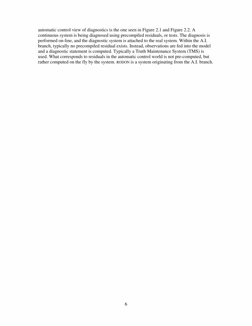
An analytical equation system can also be represented structurally as a graph. A graph consists of nodes (or vertices), and edges joining them. In Figure 3.1, equation system (3.1) is represented as a graph. In a graph, each edge has two endpoints. For example in Figure 3.1, the edge ε1 has its endpoints in the nodes {e1, x1}. All of its variables and equations are represented as nodes in the graph. There is an edge joining equation e to variable x if and only if variable x or its derivatives are present in equation e. For example the node (or equation) e1

e1: uxdt

dx+−=

21

1

e2: 212 xx = (3.1)

e3: 2xy =

8

has two edges {ε1, ε2} joining it to the variables {x1, u} since variables {x1, u} are included in equation e1.

Figure 3.1 - (3.1) as a graph

3.2 Properties of graphs

In this section, some properties of graphs will be presented. These properties will be used to formally define exactly which sets of equations we want to find using structural methods in subsequent sections. The graphs emerging when representing the structure of a system as a graph are bipartite.

Definition 3.1 (Bipartite graph): A bipartite graph is a graph that can be divided into two node sets and

where there are no edges connecting any nodes within the same set.

Figure 3.1 is an example of a bipartite graph, since it consists of two separate sets of nodes, i.e. equation nodes and variable nodes, which do not have any edges going between nodes in the same set. The nodes {x1, x2, u, y} is one of the sets. There are no edges joining any of the members of this set. Instead, the only edges present in the graph are edges joining its members to members of the other set {e1, e2, e3}. So it is a bipartite graph. We also need the notion of a matching:

Definition 3.2 (Matching): In a graph, a matching is a subset of edges such that no two edges have an

endpoint in common.

An example of a matching in Figure 3.1 would be the edges {ε1, ε4}, since they share no endpoint. An important term in this thesis is the maximum size matching, or the maximal matching:

Definition 3.3 (Maximal Matching): If the size of a matching is defined as the number of edges it includes,

a maximal matching is a matching such that its size is the greatest possible.

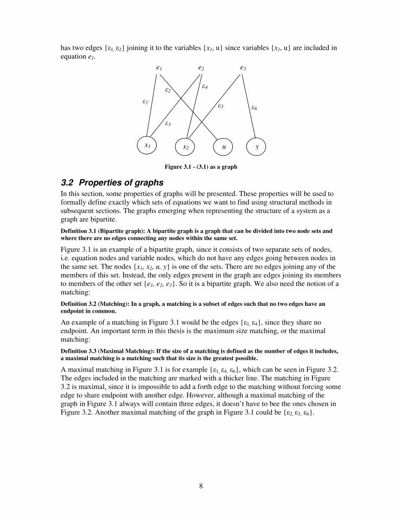
A maximal matching in Figure 3.1 is for example {ε1, ε4, ε6}, which can be seen in Figure 3.2. The edges included in the matching are marked with a thicker line. The matching in Figure 3.2 is maximal, since it is impossible to add a forth edge to the matching without forcing some edge to share endpoint with another edge. However, although a maximal matching of the graph in Figure 3.1 always will contain three edges, it doesn’t have to bee the ones chosen in Figure 3.2. Another maximal matching of the graph in Figure 3.1 could be {ε2, ε3, ε6}.

e1 e2 e3

x1 x2 u y

ε4

ε1

ε2

ε3

ε5 ε6

9

Figure 3.2 – Example of a maximal matching

3.3 Finding the overdetermined part

To use the algorithm we need a systematic approach to find the overdetermined part of a model M, since this is an important step in the structural algorithm. The overdetermined part, here denoted M+, can be found using the graph representation of a structural model described above. To determine which equations in a model M that is part of M+, we need the notions of an alternating path and a free node:

Definition 3.4 (Alternating path): Given a matching, an alternating path is a path where the edges belong

alternately to the matching and not to the matching.

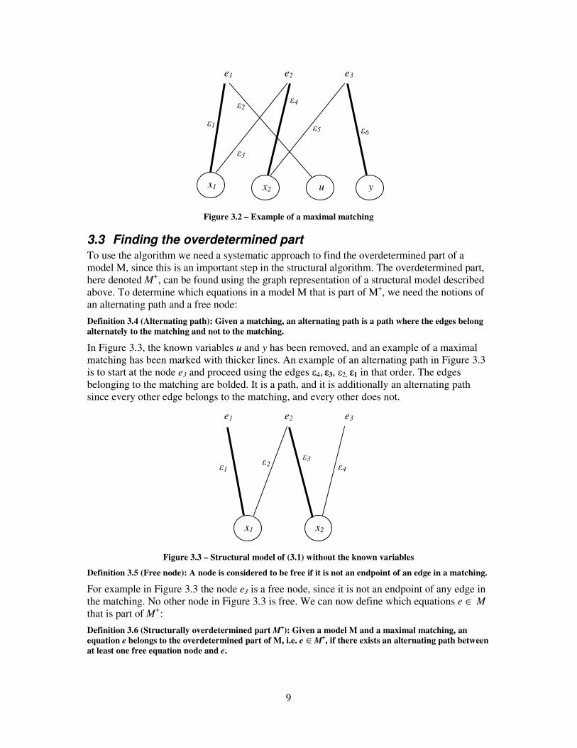
In Figure 3.3, the known variables u and y has been removed, and an example of a maximal matching has been marked with thicker lines. An example of an alternating path in Figure 3.3 is to start at the node e3 and proceed using the edges ε4, ε3, ε2, ε1 in that order. The edges belonging to the matching are bolded. It is a path, and it is additionally an alternating path since every other edge belongs to the matching, and every other does not.

Figure 3.3 – Structural model of (3.1) without the known variables

Definition 3.5 (Free node): A node is considered to be free if it is not an endpoint of an edge in a matching.

For example in Figure 3.3 the node e3 is a free node, since it is not an endpoint of any edge in the matching. No other node in Figure 3.3 is free. We can now define which equations e ∈ M that is part of M+:

Definition 3.6 (Structurally overdetermined part M+): Given a model M and a maximal matching, an

equation e belongs to the overdetermined part of M, i.e. e ∈M+, if there exists an alternating path between

at least one free equation node and e.

e1 e2 e3

x1 x2

ε1 ε2

ε3 ε4

e1 e2 e3

x1 x2 u y

ε4

ε1

ε2

ε3

ε5 ε6

10

In Figure 3.3, there is one free equation node: e3. Using an alternating path, it is possible to reach the other two equations. This means that all three equations in Figure 3.3 is part of M+.

3.4 Properties of structural models

To continue the discussion on analysis of structural models, we need to define some further properties. As mentioned before, our goal is to find parts of the system with redundancy. A set of overdetermined equations contain redundancy (Krysander, 2006). The notion structurally

overdetermined can formally be defined as follows:

Definition 3.7 (Structurally Overdetermined): A set of equations M is structurally overdetermined (SO) if

M has more equations than unknowns.

For example in Figure 3.2, there are three equations in the set M = {e1, e2, e3} and two unknowns {x1, x2} (u and y are known, as noted above). This means that the set M is structurally overdetermined, since 3 > 2. Another notion that will be useful in the following sections is the structural redundancy of a set of equations.

Definition 3.8 (Structural redundancy): The structural redundancy of a set M+

of equations is defined as

the number of equations in M minus the number of unknown variables.

For example the set {e1, e2, e3} of Figure 3.2 has three equations and two unknown variables {x1, x2}. Its structural redundancy can be calculated as (number of equations) – (number of

unknown variables) = 3 – 2 = 1. As mentioned before, we want our subsets of equations to be as small as possible, but still overdetermined. This is since smaller subsets give diagnostic tests with better isolation properties and faster computation times. Thus we can define exactly what we want as output from the structural methods. We want the Minimal Structurally

Overdetermined sets, or MSO sets. They can be formally defined as follows.

Definition 3.9 (Minimal Structurally Overdetermined): A structurally overdetermined set is a minimal

structurally overdetermined set (MSO set) if no subset is structurally overdetermined.

The set {e1, e2, e3} of Figure 3.2 has tree equations and two unknown variables. It is a SO set, and also a MSO set, since removing any of the equations would yield two equations and two unknowns, which does not comply with the demands for being an MSO set. (And not an SO set either.) This implies that the structural redundancy of an MSO set is one. The goal of the structural methods presented in this thesis is to find all MSO sets from an arbitrary structural model. An algorithm for performing this is presented in section 3.5. After having defined parts of an equation system that is of interest, the MSO sets, we can now present an algorithm for finding all MSO sets. But first let us look at how the MSO sets can be used.

3.5 Use of MSO sets in diagnostic system design

MSO sets can be used in the construction of diagnostic tests. To see how this can be done, consider the following simple model:

e1: u = x

e2: y = x A system with the input u, one internal state variable x, and an output y. The corresponding structural model in matrix form would be

11

Equation x

e1 x e2 x

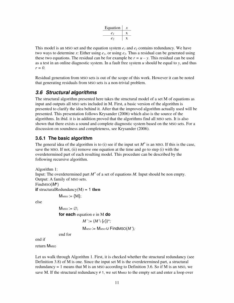
This model is an MSO set and the equation system e1 and e2 contains redundancy. We have two ways to determine x: Either using e1, or using e2. Thus a residual can be generated using these two equations. The residual can be for example be r = u – y. This residual can be used as a test in an online diagnostic system. In a fault free system u should be equal to y, and thus r = 0. Residual generation from MSO sets is out of the scope of this work. However it can be noted that generating residuals from MSO sets is a non-trivial problem.

3.6 Structural algorithms

The structural algorithm presented here takes the structural model of a set M of equations as input and outputs all MSO sets included in M. First, a basic version of the algorithm is presented to clarify the idea behind it. After that the improved algorithm actually used will be presented. This presentation follows Krysander (2006) which also is the source of the algorithms. In ibid. it is in addition proved that the algorithms find all MSO sets. It is also shown that there exists a sound and complete diagnostic system based on the MSO sets. For a discussion on soundness and completeness, see Krysander (2006).

3.6.1 The basic algorithm

The general idea of the algorithm is to (i) see if the input set M+ is an MSO. If this is the case, save the MSO. If not, (ii) remove one equation at the time and go to step (i) with the overdetermined part of each resulting model. This procedure can be described by the following recursive algorithm. Algorithm 1: Input: The overdetermined part M+ of a set of equations M. Input should be non empty. Output: A family of MSO sets. FindMSO(M+) if structuralRedundancy(M) = 1 then

MMSO := {M}; else

MMSO := ∅; for each equation e in M do

M´ := (M \ {e})+; MMSO := MMSO ∪ FindMSO(M´); end for end if

return MMSO

Let us walk through Algorithm 1. First, it is checked whether the structural redundancy (see Definition 3.8) of M is one. Since the input set M is the overdetermined part, a structural redundancy = 1 means that M is an MSO according to Definition 3.6. So if M is an MSO, we save M. If the structural redundancy ≠ 1, we set MMSO to the empty set and enter a loop over

12

the equations in M. We then remove one equation at a time, and make a recursive call with the overdetermined part of the resulting set. Let us apply Algorithm 1 to an example taken from Krysander et. al. (2005). Consider the following structural model with two unknown variables and four equations:

The example could also be conducted using a structural model of graph type, because a matrix model and a graph model both represent the same information. Here the matrix model is used since it is used in the implementation. In a structural matrix the x:s correspond to edges. A matching can be formed by selecting x:s (edges) such that there is only one x in the matching in each row and column. This corresponds to the edges in the graph representation not sharing any endpoints. The x:s marked with a circle is a possible matching in (3.1. A free equation is as said before an equation that is not an endpoint of a matched edge, that is, there is no selected x in the row corresponding to a free equation. There are two free equation nodes in ((3.1), e3 and e4. The edges, x:s, connected to them are marked with rectangles. We can now find an alternating path from the free x of the equation e3 to equation e1 and e2 by first going to the matched edge in row e2, then to the unmatched edge in the same row, and finally to the matched edge in e1. In short, we can move vertically from a non-matched edge and horizontally from a matched one. Moving vertically corresponds to being in a variable node in the graph representation and choosing any outgoing edge. Moving horizontally corresponds to standing in an equation node, and taking any outgoing edge. Using this knowledge, we can also note that we can reach equations e1 and e2 from the free edge on row e4 in the same way. This means that the structural model in (3.1) fulfills M+ = M and is therefore a valid input to Algorithm 1. Now, let us apply the algorithm. The input set is M = {e1, e2, e3, e4}. It has four equations and two variables, which gives structural redundancy 2 ≠ 1. Thus we enter the loop and remove equation e1. The resulting structure is:

A maximal matching and the free x have been marked in the new structure. Now let us find the overdetermined part of this structure. Starting from the free x, we move vertically to the matched x on row e3. Searching for unmatched x:s on this row yields no result, so we conclude that {e3, e4} is the overdetermined part. Now we recursively call the algorithm with input M = {e3, e4}. The redundancy of M is calculated. It has 2 equations. Now, since only variable x2 is present in equations {e3, e4}, it has structural redundancy 2 – 1 = 1. Apparently, {e3, e4} is an MSO, and it is saved in MMSO. Now, the algorithm continues by removing equation e2 from {e1, e2, e3, e4} which gives the same overdetermined part {e3, e4}, which still is an MSO. Next e3 is removed from {e1, e2, e3, e4}, and the MSO set {e1, e2, e4} is found. Finally, removing e4 yields the MSO set {e1, e2, e3}. The output MMSO of the algorithm is {{e3, e4}, {e3, e4}, {e1, e2, e4}, {e1, e2, e3}}.

Equation x1 x2

e1 x e2 x x e3 x e4 x

Equation x1 x2

e1 x e2 x x e3 x e4 x

(3.1)

13

3.6.2 The improved algorithm

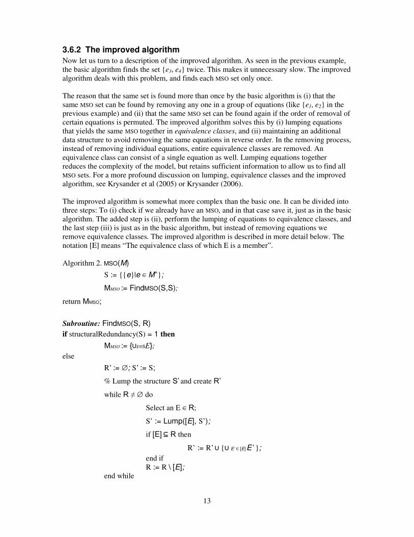
Now let us turn to a description of the improved algorithm. As seen in the previous example, the basic algorithm finds the set {e3, e4} twice. This makes it unnecessary slow. The improved algorithm deals with this problem, and finds each MSO set only once. The reason that the same set is found more than once by the basic algorithm is (i) that the same MSO set can be found by removing any one in a group of equations (like {e1, e2} in the previous example) and (ii) that the same MSO set can be found again if the order of removal of certain equations is permuted. The improved algorithm solves this by (i) lumping equations that yields the same MSO together in equivalence classes, and (ii) maintaining an additional data structure to avoid removing the same equations in reverse order. In the removing process, instead of removing individual equations, entire equivalence classes are removed. An equivalence class can consist of a single equation as well. Lumping equations together reduces the complexity of the model, but retains sufficient information to allow us to find all MSO sets. For a more profound discussion on lumping, equivalence classes and the improved algorithm, see Krysander et al (2005) or Krysander (2006). The improved algorithm is somewhat more complex than the basic one. It can be divided into three steps: To (i) check if we already have an MSO, and in that case save it, just as in the basic algorithm. The added step is (ii), perform the lumping of equations to equivalence classes, and the last step (iii) is just as in the basic algorithm, but instead of removing equations we remove equivalence classes. The improved algorithm is described in more detail below. The notation [E] means “The equivalence class of which E is a member”. Algorithm 2. MSO(M)

S := {{e}|e ∈ M+};

MMSO := FindMSO(S,S);

return MMSO;

Subroutine: FindMSO(S, R)

if structuralRedundancy(S) = 1 then

MMSO := {∪E∈SE}; else

R’ := ∅; S’ := S;

% Lump the structure S’ and create R’

while R ≠ ∅ do

Select an E ∈ R;

S’ := Lump([E], S’);

if [E] ⊆ R then

R’ := R’ ∪ {∪ E’ ∈ [E] E’ };

end if R := R \ [E]; end while

14

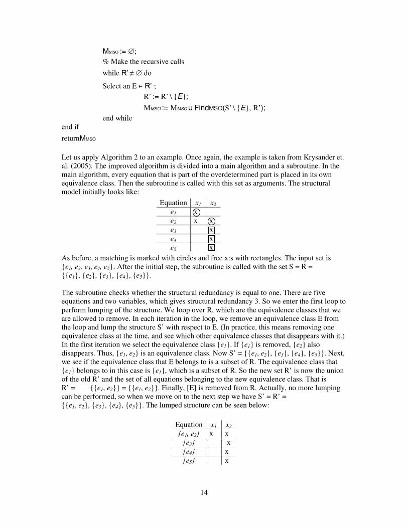
MMSO := ∅; % Make the recursive calls

while R’ ≠ ∅ do

Select an E ∈ R’ ; R’ := R’ \ {E};

MMSO := MMSO ∪ FindMSO(S’ \ {E}, R’); end while end if

returnMMSO

Let us apply Algorithm 2 to an example. Once again, the example is taken from Krysander et. al. (2005). The improved algorithm is divided into a main algorithm and a subroutine. In the main algorithm, every equation that is part of the overdetermined part is placed in its own equivalence class. Then the subroutine is called with this set as arguments. The structural model initially looks like:

As before, a matching is marked with circles and free x:s with rectangles. The input set is {e1, e2, e3, e4, e5}. After the initial step, the subroutine is called with the set S = R = {{e1}, {e2}, {e3}, {e4}, {e5}}. The subroutine checks whether the structural redundancy is equal to one. There are five equations and two variables, which gives structural redundancy 3. So we enter the first loop to perform lumping of the structure. We loop over R, which are the equivalence classes that we are allowed to remove. In each iteration in the loop, we remove an equivalence class E from the loop and lump the structure S’ with respect to E. (In practice, this means removing one equivalence class at the time, and see which other equivalence classes that disappears with it.) In the first iteration we select the equivalence class {e1}. If {e1} is removed, {e2} also disappears. Thus, {e1, e2} is an equivalence class. Now S’ = {{e1, e2}, {e3}, {e4}, {e5}}. Next, we see if the equivalence class that E belongs to is a subset of R. The equivalence class that {e1} belongs to in this case is {e1}, which is a subset of R. So the new set R’ is now the union of the old R’ and the set of all equations belonging to the new equivalence class. That is R’ = ∅ ∅ {{e1, e2}} = {{e1, e2}}. Finally, [E] is removed from R. Actually, no more lumping can be performed, so when we move on to the next step we have S’ = R’ = {{e1, e2}, {e3}, {e4}, {e5}}. The lumped structure can be seen below:

Equation x1 x2

{e1, e2} x x {e3} x {e4} x {e5} x

Equation x1 x2

e1 x e2 x x e3 x e4 x e5 x

15

We now make the recursive call removing one equivalence class at a time. The loop starts by selecting an equivalence class from R’. We select the first one, {e1, e2}. It is removed from R’, and the subroutine is called again with S’ \ {E} and R’. In this case it would be S’ \ {{e1, e2}} = R’ = {{e3}, {e4}, {e5}}. Note that E is permanently removed from R’. This is to prevent permuted removal orders. The loop continues, and in the next iteration it will select {e3} and call the subroutine with S’ \ {e3} = {{e1, e2}, {e4}, {e5}} and R’ = {{e4}, {e5}}. The final output is {{e4, e5}, {e3, e5}, {e3, e4}, {e1, e2, e5}, {e1, e2, e4}, {e1, e2, e3}}. To further illustrate how the algorithm works, Algoritm 2 is applied to a larger example taken from Krysander (2006). The input to the structural algorithm is as follows:

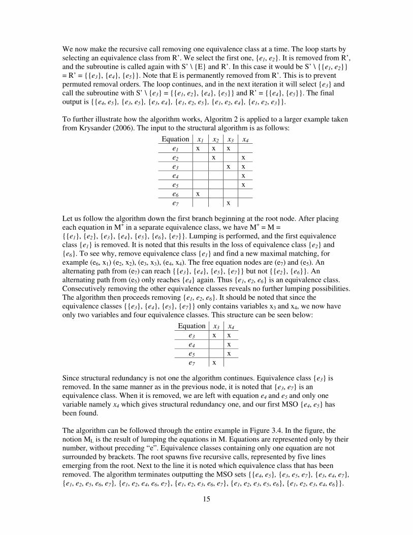
Let us follow the algorithm down the first branch beginning at the root node. After placing each equation in M+ in a separate equivalence class, we have M+ = M = {{e1}, {e2}, {e3}, {e4}, {e5}, {e6}, {e7}}. Lumping is performed, and the first equivalence class {e1} is removed. It is noted that this results in the loss of equivalence class {e2} and {e6}. To see why, remove equivalence class {e1} and find a new maximal matching, for example (e6, x1) (e2, x2), (e3, x3), (e4, x4). The free equation nodes are (e7) and (e5). An alternating path from (e7) can reach {{e3}, {e4}, {e5}, {e7}} but not {{e2}, {e6}}. An alternating path from (e5) only reaches {e4} again. Thus {e1, e2, e6} is an equivalence class. Consecutively removing the other equivalence classes reveals no further lumping possibilities. The algorithm then proceeds removing {e1, e2, e6}. It should be noted that since the equivalence classes {{e3}, {e4}, {e5}, {e7}} only contains variables x3 and x4, we now have only two variables and four equivalence classes. This structure can be seen below:

Since structural redundancy is not one the algorithm continues. Equivalence class {e3} is removed. In the same manner as in the previous node, it is noted that {e3, e7} is an equivalence class. When it is removed, we are left with equation e4 and e5 and only one variable namely x4 which gives structural redundancy one, and our first MSO {e4, e5} has been found. The algorithm can be followed through the entire example in Figure 3.4. In the figure, the notion ML is the result of lumping the equations in M. Equations are represented only by their number, without preceding “e”. Equivalence classes containing only one equation are not surrounded by brackets. The root spawns five recursive calls, represented by five lines emerging from the root. Next to the line it is noted which equivalence class that has been removed. The algorithm terminates outputting the MSO sets {{e4, e5}, {e3, e5, e7}, {e3, e4, e7},

{e1, e2, e5, e6, e7}, {e1, e2, e4, e6, e7}, {e1, e2, e3, e6, e7}, {e1, e2, e3, e5, e6}, {e1, e2, e3, e4, e6}}.

Equation x1 x2 x3 x4

e1 x x x e2 x x e3 x x e4 x e5 x e6 x e7 x

Equation x3 x4

e3 x x e4 x e5 x e7 x

16

Figure 3.4 - Application of Algorithm 2 to a larger example

M+ = {3,4,5,7} ML = R = {{3,7},4,5}

{1,2,6}

MSO: {4,5}

{3,7}

MSO: {3,5,7}

M+ = {{1,2,6},4,5,7} ML = {{1,2,6,7},4,5} R = {4,5}

{3}

MSO: {1,2,5,6,7}

MSO: {1,2,4,6,7}

{4}

{4} {5}

{5}

M+ = ML = {{1,2,6},3,5,7} R = {5,7}

{4}

{5}

MSO: {1,2,3,6,7}

{7}

MSO: {1,2,3,5,6}

M+ = ML = {{1,2,6},3,4,7} R = {7}

{5}

{7}

MSO: {1,2,3,4,6}

M+ = ML = {{1,2,6},3,4,5} R = {}

{7}

MSO: {3,4,7}

M+ = {1,2,3,4,5,6,7} ML = R = {{1,2,6},3,4,5,7}

{4}

17

4 RODON This chapter introduces the software RODON. It describes its basic features, its modeling language Rodelica and some special elements of that modeling language. RODON is a software diagnostics tool. It can be used for reliability calculations, failure mode and effect analysis, fault isolation, and more. RODON is based on a component-based model of the system. The model is described in a language called Rodelica. The model typically also contains information about the failure modes of each component, and the alternative behavior of the model in each failure mode.

4.1 Rodelica

Rodelica is the modeling language of RODON. It is an object oriented, equation based language that is very close to Modelica (Lunde, 2000). Modelica is developed and promoted by the Modelica Association, and further details can be found in (Modelica, 2007). Rodelica has some additional features to adapt it better to diagnosis purposes, for example the OR-clause mentioned below. For a more profound discussion on the additional features of Rodelica, see Lunde (2000). Below the Rodelica code from a rudimentary resistor is presented. // Copyright Sörman information & media AB // ======================================================================== /** Model of a basic ohmic resistor without any failure modes.<br><br> <b>This model should only be used to model equivalent circuits resp. in cases, when the model has no physical counterpart in reality.</b><br><br> @author Sörman information & media AB */ // ======================================================================== model ResistorBasic // ======================================================================== public /** Electrical pin 1 of component. */ Pin p1; /** Electrical pin 2 of component. */ Pin p2; /** Nominal resistance between both pins.<br><br> <u>Definition range of parameter:</u><br> rNom &gt; 0. */ Resistance rNom(final min = 0); // ------------------------------------------------------------------------ behavior // ------------------------------------------------------------------------ // Current balance: Kirchhoff(p1.i, p2.i); //Voltage drop between pin 1 and pin 2 Ohm(p1.u, p2.u, p1.i, rNom); // ======================================================================== end ResistorBasic; // ========================================================================

This code snippet is provided only as a brief example of what Rodelica code may look like, and no further dissection will be performed in this report. For further information on Rodelica see Lunde (2002).

18

4.2 Simulation in RODON

The RODON model is described by constraints. Constraints are relations between model variables. They are typically physical laws. In this work constraints and equations are used interchangeably if it is not explicitly stated otherwise. However, the RODON notion of a constraint is actually more general than an equation. To simulate the system, all constraints and variables are connected in a constraint network. The constraint network contains information about which variables that depend on which constraints. By iterating through the constraint network, and applying all constraints that apply for each variable, the simulation engine can simulate the model.

4.3 Model characteristics

Quantities are typically represented as intervals in RODON. This is preferred since it enables the system to represent uncertainties. When dealing with real systems, measurements always contain uncertainties. Furthermore, component manufacturers typically give data as tolerances (Lunde, 2000). Modeling in RODON is non-directional, in contrast to other simulation tools such as Simulink. This means that if some component has a failure mode “short to ground”, current can take an unintended direction via other components to the shortage. This behaviour can be represented in a single RODON model. This is not possible in the directional modeling paradigm.

4.3.1 The OR Clause

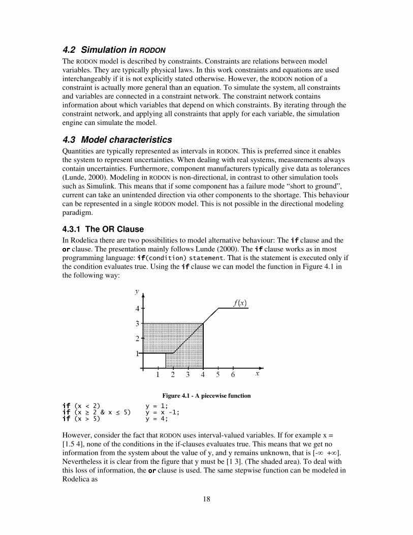
In Rodelica there are two possibilities to model alternative behaviour: The ifififif clause and the orororor clause. The presentation mainly follows Lunde (2000). The ifififif clause works as in most programming language: ifififif(condition) statement. That is the statement is executed only if the condition evaluates true. Using the ifififif clause we can model the function in Figure 4.1 in the following way:

Figure 4.1 - A piecewise function

ifififif (x < 2) y = 1; ifififif (x ≥ 2 & x ≤ 5) y = x -1; ifififif (x > 5) y = 4;

However, consider the fact that RODON uses interval-valued variables. If for example x = [1.5 4], none of the conditions in the if-clauses evaluates true. This means that we get no information from the system about the value of y, and y remains unknown, that is [-∞ +∞]. Nevertheless it is clear from the figure that y must be [1 3]. (The shaded area). To deal with this loss of information, the orororor clause is used. The same stepwise function can be modeled in Rodelica as

19

orororor { {x < 2; y = 1;} {x = [2 5]; y = x -1;}

{x > 5; y = 4;} }

The evaluation of the or clause is as follows: Each of the subsets is evaluated. If all statements within a subset are consistent with the information currently held about the state of the model, the subsets are saved. Otherwise it is discarded. When all subsets have been evaluated, the union of the saved ones is used in the propagation. It is treated as one complex constraint by RODON. In the example above where x = [1.5 4], the evaluation would start by looking at the first subset. Is it possible that x < 2 ? Certainly, as x might be 1.6 for example. Is it possible that y = 1? As well, since we assume that y is unknown and can obtain any value. Thus, the first subset is valid, and saved. In the same way, it is noted that the second subset contains a statement that x = [2 4]. This is also possible, as well as the statement about y, since all statements about y are true. The second subset is saved. Evaluating the third subset, we note that the statement x > 5 is inconsistent with our current knowledge about x, which says it is not higher then 4. The third subset is thus discarded. Apparently we should take the union of the first and second subset. This means considering y = 1 and y = x -1 = [2 4] -1 = [1 3]. This corresponds the result shown in Figure 4.1.

4.4 Model classes

The modeler of a Rodelica model is quite free in her design. Models can be under-constrained, just-constrained and over-constrained. This is a strength which adds flexibility to the system. In the case of underdetermined models, the simulation engine obviously cannot determine all variables exactly. However, since real numbers in RODON typically are represented as intervals, it can possibly narrow down the feasible intervals that the variables can attain. For justconstrained and overconstrained systems, it can determine all variables exactly, as expected. Overconstraining the system can mean faster simulation, since the search space is limited. Although these features are advantageous in many cases, it presents problems for the structural algorithms as noted below.

4.5 Modeling in RODON

RODON uses an object oriented approach to modeling. This provides for scalability and reuse of code. Modeling in RODON typically implies constructing, or re-using an already existing modeling library. RODON has a number of predefined model libraries for areas such as electric models and logic models. In Figure 4.2 a view from the electrical library in RODON is shown.

20

Figure 4.2 - The RODON electrical library with the package “Resistors” open

21

5 STRUCTURAL ALGORITHM PROTOTYPES IN RODON One important part of this thesis project was to implement a prototype and integrate it into RODON. In this chapter the implemented prototype is described. It is described how the equations and variables are extracted out of a RODON model, and how the algorithms are implemented. It also features an application of the prototype to a small example model. A large part of this thesis work has been to implement a structural algorithm prototype as a module in RODON. This work can be divided into two parts: To implement a program to extract a structural model from a RODON model, and to implement the structural algorithms. The procedure for using structural algorithms in RODON can be described as follows: (a) Extract an equation system and construct a structural model (b) apply structural algorithms and extract the MSO sets. Instead of using a sensor component and include it into the models, a interface where the user of the structural prototype can add sensors to the model at runtime has been chosen. This solution enables the user to experiment with different sensor placement without reconstructing the model. It also provides a possibility to apply structural methods to already existing RODON models that does not contain any sensors. This interface adds a step between (a) and (b) consisting of choosing which quantities to measure. The programming has been performed using the java programming language in the Eclipse programming environment. In many cases the RODON model is overdetermined by the modeler. Extra information has been added to the model. However this information has nothing to do with the sensor information. When using structural models the overdetermination of the system should come from sensors in the system. Thus some equations might have to be removed. Then, at runtime, equations that correspond to an imagined sensor placement are added to overdetermine the system anew. Models that contain sensor components have not been taken into account in the prototype, mainly since the example models used does not contain sensors.

5.1 Extracting equations and variables

Since we assume a model with no existing sensors in it, the goal of this step is to extract a just constrained equation system from the RODON constraint net. A just constrained equation system is a system with the same number of equations as unknown variables. It has shown to be non trivial to automatically select which variables and equations in the RODON constraint network that should be included in the structural model for arbitrary models.

5.1.1 Challenges in extracting variables

For example, there are condition variables used to describe the model behavior in case of failure. A Rodelica constraint can for example be

if (fm == 0) p1.u - p2.u = p1.i * rAct; which means: If the current component is in failure mode 0, (the no fault case), the voltage in pin 1 minus the voltage of pin 2 is equal to the current in pin 1 times the actual resistance. (Ohms law) In this case the first variable fm should not be included in the structural model. This is since it is only used to determine in what mode the system is in, and does contain information about the system itself. The variable should not be included either, since it is a known variable. Although this example is a trivial problem, the fact that the Rodelica modeler has a great degree of freedom means that we can be confronted by very different kinds of models. This topic will be treated in more systematically in section 5.1.3.

22

5.1.2 Challenges in extracting equations

The modeler can for example decide that some variable in some case will always be greater than 0, and simply add that as a constraint. Why is such an overdetermined system, overdetermined by inequalities, not appreciated? Consider the following simple model of a system:

e1: u = x

e2: y = x The model contains two equations and one unknown variable x. Now assume that the modeller adds a third equation:

e3: x > 0 Looking at the structural model,

Equation x

e1 x e2 x e3 x

it seems that we have three ways to determine x, and a structural redundancy of two. Running the MSO algorithm on this structural model yields the MSO sets {{e1, e2}, {e1, e3}, {e2, e3}}. What diagnostic tests can be constructed from these MSO sets? From the first MSO set {e1, e2} a residual can be created, for example u – y = 0. However the second and third sets present problems. Using the second set for example, we can not determine x in two ways using equation e1 and e3. It could be used as a residual, and we could detect for example if x falls below 0, but it is far from the sensitivity of the residual created from the first MSO set. This kind of low sensitivity residual does not contain as much information. Since the algorithm runs into complexity problems when redundancy is high, focusing a high information residuals is the chosen approach. Why can not inequalities simply be removed from the equation system? Although this would produce a just constrained model as desired in some cases, as the one presented above, it is not feasible for all cases. For example there are other types of models where inequalities are used to set other variables. A discrete sound variable can for example be set to 1 (that is emitting sound) if the current through a signal horn surpasses a certain threshold. Another challenge is the or clause. As noted above, it is a special constraint type that needs processing before use. Due to the time constraints of this work, a full treatment of the or-clause has not been implemented. Further development of this is needed. See Chapter 7 for future work. Other challenges not addressed in this work are constraints in the form of splines and lookup tables. An outline for treatment of these is presented in Chapter 7. Because of the freedom of the modeler, exemplified by the cases presented here, selecting the proper equations from the RODON model has shown to be the most difficult part of this thesis.

5.1.3 Actual implementation

The implemented selection of constraints and variables is based on a heuristic approach, and it does not produce correct results for arbitrary models. Further below some modeling guidelines will be presented, which can be used to create models where a correct structural model can be extracted in a straightforward manner. The extraction is performed by looping through all constraints. Constraints that do not have conditions are added to the structural

23

model. Constraints with conditions are added only after its condition has been evaluated true. For example, the constraint

if (fm == 0) p1.u - p2.u = p1.i * rAct;

would be added only if the condition (fm == 0) is true, that is we have chosen to run the algorithm on the no-fault model. For each added constraint, the variables used are sent to a variable manager. A variable is added to the list of structural model variables if it fulfils the following conditions: a) It is not a known variable. Only unknown variables are stored in the structural model. b) It is not a failure mode variable. c) It is not already in the list. The same variable typically exists in various constraints. Finally, a structural model matrix in the form of a two dimensional array is created.

5.2 Implementation of structural algorithms

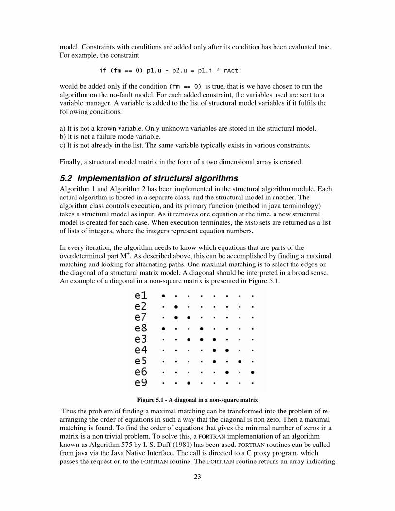
Algorithm 1 and Algorithm 2 has been implemented in the structural algorithm module. Each actual algorithm is hosted in a separate class, and the structural model in another. The algorithm class controls execution, and its primary function (method in java terminology) takes a structural model as input. As it removes one equation at the time, a new structural model is created for each case. When execution terminates, the MSO sets are returned as a list of lists of integers, where the integers represent equation numbers. In every iteration, the algorithm needs to know which equations that are parts of the overdetermined part M+. As described above, this can be accomplished by finding a maximal matching and looking for alternating paths. One maximal matching is to select the edges on the diagonal of a structural matrix model. A diagonal should be interpreted in a broad sense. An example of a diagonal in a non-square matrix is presented in Figure 5.1.

Figure 5.1 - A diagonal in a non-square matrix

Thus the problem of finding a maximal matching can be transformed into the problem of re-arranging the order of equations in such a way that the diagonal is non zero. Then a maximal matching is found. To find the order of equations that gives the minimal number of zeros in a matrix is a non trivial problem. To solve this, a FORTRAN implementation of an algorithm known as Algorithm 575 by I. S. Duff (1981) has been used. FORTRAN routines can be called from java via the Java Native Interface. The call is directed to a C proxy program, which passes the request on to the FORTRAN routine. The FORTRAN routine returns an array indicating

24

how to re-arrange the rows in the matrix to arrive at zero-free diagonal if possible. The matrix is re-arranged according to this array. To find alternating paths an intuitive approach has been taken, where a path is searched for from each free node. This has shown to be a very slow approach. There are efficient algorithms for doing both the matching step and more, for example the Dulmage-Mendelsohn permutation (Dulmage & Mendelsohn, 1958) algorithm implementation in Matlab, DMPERM. A java implementation of this algorithm has not been found, and it has not been performed in this thesis due to time constraints.

5.3 Application to an example

In this section the structural prototype will be applied to a RODON model step by step. Let us start with the following rudimentary RODON model named TestClass consisting of a battery, a resistor, and a ground node.

Figure 5.2 - A rudimentary RODON model

The RODON constraint net provides the following constraints for this model:

1. ground: if (fm == 0) p.u = 0; 2. ground: if (fm == 1) p.i = 0; 3. battery: if (mode == 0) p.u = Tutorial.EEBasics.U_VCC; 4. battery: if (mode == 1) p.u - Tutorial.EEBasics.U_VCC = p.i * r; 5. resistor: if (fm == 0) p1.u - p2.u = p1.i * r; 6. resistor: p1.i + p2.i = 0; 7. resistor: if (fm == 1) p1.i = 0; 8. testClass: battery.p.i + resistor.p1.i = 0; 9. testClass: resistor.p2.i + ground.p.i = 0; 10. testClass: battery.p.u - resistor.p1.u = 0; 11. testClass: ground.p.u - resistor.p2.u = 0;

Each component has a number of constraints defining its internal behavior, namely constraint 1 to 7. Each component has alternative behaviors for different failure modes. For example, the ground node has two constraints, 1 and 2. The first one states that if the failure mode is 0, that is the no fault mode, the potential is 0. If the ground node is in failure mode 1, that is disconnected, no current will enter its pin. There are also four connector statements belonging to the model as a whole, defining how the components are interconnected. In these connector statements the variables are named in a global namespace, that is they are preceded with their component name. Tutorial.EEBasics.U_VCC is a known constant. Since components must exclusively be in one failure mode, the equation system presented above cannot be used to create a structural model. Such a structural model would contain logical inconsistencies, like statements claiming the system is in two operational modes that are mutually exclusive. Let us therefore set the failure modes of all components to one mode,

25

the no fault mode. The battery has a mode variable which can be set to ideal or linear. We set the mode to ideal, that is its voltage is equal to Tutorial.EEBasics.U_VCC. This yields: Eq 1: ground: if (fm == 0) p.u = 0; Eq 2: battery: if (mode == 0) p.u = Tutorial.EEBasics.U_VCC; Eq 3: resistor: if (fm == 0) p1.u - p2.u = p1.i * r; Eq 4: resistor: p1.i + p2.i = 0; Eq 5: testClass: battery.p.i + resistor.p1.i = 0; Eq 6: testClass: resistor.p2.i + ground.p.i = 0; Eq 7: battery.p.u - resistor.p1.u = 0; Eq 8: ground.p.u - resistor.p2.u = 0;

Now let us look at the variables. Typically each pin of each component has a current and a voltage variable. There are also some additional variables. The constraint network for the model TestClass contains the following 13 variables: ground.p.u ground.p.i ground.fm* battery.p.u battery.p.i

battery.mode* battery.r* resistor.r* resistor.p1.u resistor.p1.i

resistor.p2.u resistor.p2.i resistor.fm*

Since we have decided that all components are in the no fault mode, the failure mode variables are known. Since the structural models used in this thesis only considers the unknown variables, they are not of interest and should not be included in the just constrained structural model of the system. Further more they are not really model variables, but merely used to decide which constraint should be included in the current model and not. Two more variables are not of interest in the structural model with only unknown variables namely battery.r and resistor.r, which are known constants. Battery.r is the internal resistance of the battery, and is used if the battery is used in linear mode. It should not be a part of the structural model since we use the battery in ideal mode. Resistor.r is the nominal resistance of the resistor, and it is not included since it is a known scalar, in this case we have set it to 10 Ohm. Removing the variables mentioned above, (marked with *) the following 8 remain: Var 1: ground.p.u Var 2: battery.p.u Var 3: resistor.p1.u

Var 4: resistor.p2.u Var 5: resistor.p1.i Var 6: resistor.p2.i

Var 7: battery.p.i Var 8: ground.p.i

We now have a just constrained system, and we have 8 equations and 8 unknown variables. The resulting structural model with structural redundancy 0 is

Figure 5.3 – A structural representation of the TestClass model

26

In Figure 5.3 a large dot in place (i, j) (row, column) means that variable j is present in equation i. For example equation number 1 contains the variable 1 (ground.p.u) and consequently there is a large dot in place (1,1) in the matrix. Now let us make the system overdetermined. This corresponds to placing virtual sensors in the model, measuring the quantity. As noted above, redundancy is needed to be able to diagnose a system. Choosing where to place the sensor(s) is done in a dialog box as seen in Figure 5.4.

Figure 5.4 - The variable selection dialog in the structural prototype

Assume we select the variable resistor.p1.u. This corresponds to adding another equation including resistor.p1.u to the structural model. Thus we now have a total of 9 equations, where the ninth can be represented as Eq 9: resistor.p1.u = measuredBySensor;. The notation measuredBySensor means that a sensor is measuring the quantity on the other side of the equal sign. The structural matrix resulting from selecting variable resistor.p1.u and rearranging the equations so that the matrix has a non-zero diagonal can be seen in Figure 5.5. Rearrangement of the equations to a non-zero diagonal is done since the diagonal represents a matching, as noted above.

Figure 5.5 - Structural matrix of TestClass model one sensor measuring resistor.p1.uresistor.p1.uresistor.p1.uresistor.p1.u added

27

The structural algorithm terminates outputting one MSO set namely {2, 7, 9}. That means that the three equations in the MSO set together contain redundancy, and they can be used to construct a residual. Let us recall equations 2, 7 and 9: Eq 2: battery: if (mode == 0) p.u = Tutorial.EEBasics.U_VCC; Eq 7: battery.p.u - resistor.p1.u = 0; Eq 9: resistor.p1.u = measuredBySensor;

Using variable elimination, we can conclude that a possible residual r is

r = Tutorial.EEBasics.U_VCC – measuredBySensor = 0

Adding some threshold to handle measurement noise, this could be a possible test to run in an online diagnostic system.

5.4 Limitations of the prototype

Due to the difficulties mentioned above to extract a well constrained equation system from a RODON model the prototype does not work for all RODON models. It only works for a small subset of components in the RODON tutorial.EEBasics library. The tutorial.EEBasic library contains components modeled in less detail then the standard electrical library, and is intended for training only. For a list of compatible components, see Appendix 1. There is also a limitation on the input set M: It must not contain any underdetermined part. This is due to implementation issues, and can be solved by replacing the algorithms used to find the overdetermined part. See also Chapter 7.

5.5 Modeling guidelines

This section contains some facts that can facilitate the extraction of a structural model from a RODON model. For example, the equations belonging to the just constrained system could be marked in a certain way. Another possibility is to only include the equations belonging to the just constrained system, like in the tutorial library mentioned above. However this of course greatly limits the use of the Rodelica modeling language.

5.6 Empirical time complexity analysis

Here the results from a simple time complexity analysis are presented. It is compared how execution time increase when varying the number of equations and the redundancy.

28

5.6.1 Dependence on the number of equations

Theoretically the algorithm scales very well with increases in the system size with fixed redundancy, resulting in only a low polynomial increase in time demands. This has been tested empirically using resistors connected in series. The number of resistors has been increased in steps of five. Three executions have been performed at each system size, and the average time has been used. The result can be seen in Figure 5.6. As can be noted, the results fit well to the expectations of a low order polynomial growth in execution time.

0

100

200

300

400

500

600

700

800

900

1000

0 50 100 150 200

Number of equations

Execu

tio

n t

ime (

ms)

Figure 5.6 - Execution time as a function the number of equations

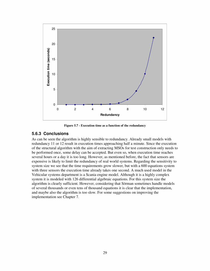
5.6.2 Dependence on redundancy

As noted above the algorithm theoretically has an exponential increase in execution time when redundancy is increased and the number of unknowns is held constant. This has been tested in the actual implementation by using a system consisting of one battery, 4 resistors in parallel and a ground node, and increasing the redundancy in steps of one. Three test runs has been made at each redundancy, and the average time is presented in the Figure 5.7. The result again matches the expectations with an exponential growth in execution time.

29

0

5

10

15

20

25

0 2 4 6 8 10 12

Redundancy

Execu

tio

n t

ime (

seco

nd

s)

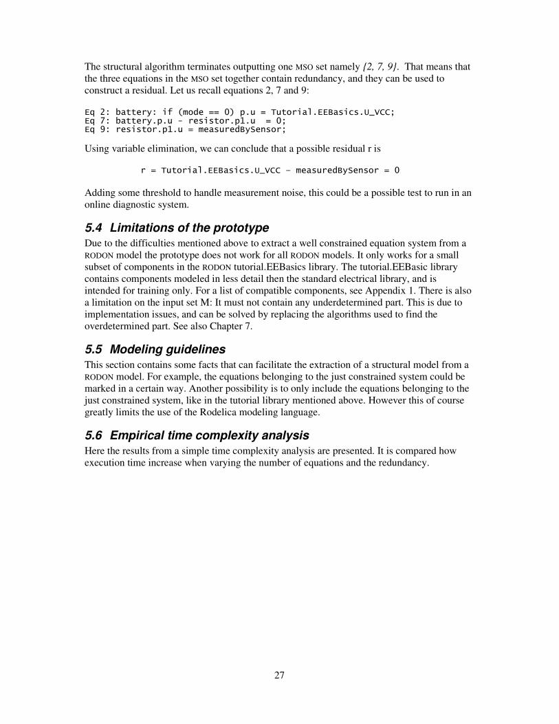
Figure 5.7 - Execution time as a function of the redundancy

5.6.3 Conclusions

As can be seen the algorithm is highly sensible to redundancy. Already small models with redundancy 11 or 12 result in execution times approaching half a minute. Since the execution of the structural algorithm with the aim of extracting MSOs for test construction only needs to be performed once, some delay can be accepted. But even so, when execution time reaches several hours or a day it is too long. However, as mentioned before, the fact that sensors are expensive is likely to limit the redundancy of real world systems. Regarding the sensitivity to system size we see that the time requirements grow slower, but with a 600 equations system with three sensors the execution time already takes one second. A much used model in the Vehicular systems department is a Scania engine model. Although it is a highly complex system it is modeled with 126 differential algebraic equations. For this system size the algorithm is clearly sufficient. However, considering that Sörman sometimes handle models of several thousands or even tens of thousand equations it is clear that the implementation, and maybe also the algorithm is too slow. For some suggestions on improving the implementation see Chapter 7.

30

31

6 OTHER USES OF STRUCTURAL ALGORITHMS IN RODON This chapter features the interview results regarding other possible uses of structural methods. The use of structural methods advocated throughout this thesis is for diagnostic test construction. However a part of the problem formulation was to investigate other possible uses of structural methods in RODON. This investigation has been performed by interviewing two groups of people, namely employees at Sörman working with RODON, and researchers at Vehicular Systems Department. The results of these interviews are compiled and presented in this chapter.

6.1 Interview results from employees at Sörman

One suggestion was that structural methods could be used to find out which components that are possible to monitor given a sensor in a certain position. The components that are part of a certain MSO are in some way related. However a failure in a component not in the MSO can not be detected by the sensor. By performing structural methods on a system, it can be determined if failure in a certain component can be “seen” using a sensor, a task that can be difficult to perform manually if the system is large and complicated. Another suggestion was to use structural methods to decide which subparts of the model to model in more detail. Assume that first a general, not very detailed model of a large system is constructed. This can be done in Rodelica, or in some other modeling language. By running structural methods on this model, it can be seen which parts of the system interact, and which are dependent upon another. It can also show which parts that contain redundancy. In a situation where the modeler knows that some parts are of more interest then others, he can use these criteria to divide the model into suitable subparts with redundancy. These subparts can then be modeled in more detail for example in RODON. It was also suggested that the work done in this thesis to extract a well constrained equation system from a RODON model could be used. The resulting equation system could then be fed to a fast, numerical solver to provide for faster simulation. Although this is not a use of structural methods in RODON, it is a possibility to use other parts of the work in this thesis, and the suggestion is therefore included. As noted above, the process of extracting a well constrained equation system from a RODON model has not been successful for the general case, but merely for a very limited subset of the model library. In a similar way, the knowledge about which equations are part of the just constrained system could be used to create a meta modeling language. This would be a super class to Rodelica, which contains everything Rodelica contains, but also information about which equations are part of the just constrained model. The idea here is as above to feed the just constrained part to a faster simulation engine.

6.2 Interview results from researchers at Vehicular Systems Department

One use of structural methods is detectability and isolability analysis. Given the structure of a system a fault incidence matrix can be constructed. A fault incidence matrix is a representation of the sensibility to different faults by diagnostic tests. For example:

32

It follows that test t1 reacts to fault f2 and only fault f2. However test t2 reacts to both fault f1

and f2. The problem solved with detectability and isolability analysis can be summed up as: Given a system with certain sensors, find the diagnostic performance. This can be seen as the inverse of another problem where structural methods are useful: Given a system and a desired fault detectability and isolability how many sensors are needed and where should they be placed? This can be denoted the sensor placement problem. Consider for example the following structural model:

The system consists of two equations, each one sensible to one fault. There is no redundancy. The sensor placement problem is: Where should an additional sensor be placed to achieve best possible isolation properties? There are two options: Measuring x1 and measuring x2. Using structural analysis we can quickly see what properties are obtained in the two cases. For example let us measure x2 and include in the model as an additional equation containing x2. The only MSO set would be {e2, e3}. This means that a diagnostic system using the test derived from this set would only be sensible to f2. Instead consider measuring x1. Now {e1, e2, e3} is an MSO set. This means that the residual can be sensible to both f1 and f2. We conclude that placing a sensor that measures x1 gives the best diagnostic performance. For further reading in sensor placement using structural methods see Raghuraj et al, (1999). Structural methods can also be used to determine which faults in a system model that needs further modeling to obtain the desired diagnostic system performance. This is an alternative to adding more sensors. However modeling faults in detail is a difficult task that requires detailed engineering knowledge of the components. A small example inspired by Frisk et. al. (2003) illustrates how fault modeling can be used. The following system has two equations and three unknown signals: The internal state variable x1 and the unknown faults f1 and f2.

Since there is no structural redundancy there are no MSO sets. Now assume that we know that the first derivative of f1 is 0, that is it increases very slowly or is constant within some time interval. Using the same methods as above, that is treating time derivatives of variables and variables as the same, the following structure is obtained:

Now it is possible to isolate fault f1 from fault f2. A more profound discussion can be found in Frisk et al. (2003). Another use of structural methods surges if an observer is used to form a diagnostic test. Then an observability analysis using structural methods can be conducted first. The observability problem is: Under what conditions can the internal state of a system be reconstructed by

Equation Sensible to x1 x2

e1 f1 x x e2 f2 x

Diagnostic test f1 f2

t1 0 x t2 x x

Equation x1 f1 f2

e1 x x x e2 x

Equation x1 f1 f2

e1 x x x e2 x e3 x

33

knowing only the input and output of a system during a limited time? Assume that the structural analysis gives that the system is observable. An observer is constructed. Now structural methods can be used again to determine what part of the system that needs to be accounted for in the observer. Lastly assume that the system contains some relation that is difficult to model. One example is how the temperature in one place depends on the rest of the system. Then structural methods can be applied, and it is possible to see what parts of the model that contains this modeling difficulty, and which does not. Then a detectability and isolability analysis can be performed on the parts, the MSOs, without the difficulty. Can sufficient diagnostic performance be obtained without modeling the difficult part? If so, we can avoid having to model the difficult behavior in more detail, and simply design the diagnostic system based on the MSOs without the difficult part.

6.3 Summary and comments

The first suggestion by Sörman employees, using structural analysis to see what components that can be monitored by a certain sensor, is basically what is called isolability analysis in this thesis, and it is certainly a possible use of structural methods in RODON. The second suggestion, using structural methods to divide the model into subparts, might also be a possible use, but more research is needed in this area. The third and fourth suggestions are not really uses of structural methods, but uses of the first part of the task: Extracting an equation system. The suggestion is to use this knowledge to perform high speed simulation. They are certainly interesting options if the task of extracting a structural method out of RODON can be performed successfully. Of the suggestions by ISY researchers, sensor placement is an interesting application for use in RODON. Performing fault isolability analysis can also be of interest. Also fault modeling might be of use for the RODON modeler.

34

35

7 DISCUSSION AND FUTURE WORK The original objective of this thesis was to apply structural algorithms to arbitrary RODON models. This has not been met, due to difficulties extracting the just constrained equation system. Some heuristic approaches has been taken, none of which has given sufficiently satisfying results. However I think that it might be possible to implement a satisfying algorithm for variable extraction. Research in the field can be applied, for example methods from Bunus (2004). Even though it probably isn’t possible to account for all models possible to make in Rodelica, it can be possible for a sufficiently large subset of the models. The or-clause can probably also be dealt with by evaluating all the constraints in each bracket, extracting the ones consistent with the current environment and finally creating new constraints for each valid constraint in the or-clause. The other types of constraints, namely splines and lookup tables should not present a problem. The variables included in the table can be entered into the structural model. Actually, dealing with lookup tables is one of the advantages of structural methods over analytical ones according to Krysander (2006). Moreover the speed of the algorithm can be increased. The main bottleneck of the implementation is the code that finds the overdetermined part in the system. This is done by rearranging the equations with the external FORTRAN routine, and then following an intuitive approach to find the overdetermined part. A much faster way would be to write or find a java implementation of the DMPERM command of MatLab or similar, that can perform both tasks fast. Improving the code that extracts the overdetermined part has the additional advantage of ridding the program of a restriction on the input: That no underdetermined part is allowed in the input set. All internal matrix handling should furthermore be performed in the sparse matrix format to increase speed. Today, two-dimensional arrays as well as sparse matrix format are used. The two-dimensional array representation is slower and consumes unnecessary memory. It has been used in the prototype since it is much more human readable than the sparse matrix format. One question that naturally surges is: Should the development of structural methods in RODON be continued? Some aspects to consider are these: Even if an additional effort is made to extend the scope of the implemented prototype to cover a sufficiently large subset, much work remains before actual residuals can be inserted as diagnostic tests in an online diagnostic system. Automatic residual generation from MSO sets is a non-trivial task. If the development is continued, other uses of structural methods then residual generation should also be considered. For example optimal sensor placement might be a less complex use of structural methods in RODON.

36

37

8 CONCLUSIONS The work conducted in this thesis has shown that it is possible to apply structural methods to RODON models. It has also shown that even a prototype implementation can handle quite large systems. Some problems have also been found during the project. Extracting a structural model from RODON models is not a straightforward process. This is due to the ability of RODON to handle under-, just- and over-constrained models. Therefore the implemented prototype only works for a small subset of especially rudimentary models in the modeling library. Spending more time on the task can certainly increase this subset. It can probably make it sufficiently large to make structural methods useful in RODON. However, it will likely be difficult to extend the subset to the set of all possible RODON models, due to the freedom of the modeler in Rodelica. The implemented algorithm can handle reasonably big systems as long as redundancy is low. The prototype performance has good potential for improvements, most notably in the algorithm to find the overconstrained part of a model. Improving this part will have great impact on execution speed. It can also extend the valid input set. The main use of structural methods considered here has been to find suitable residuals to create diagnostic tests. However other uses of structural methods have been investigated as well. Many of these can be used in RODON if a structural model can be extracted successfully. For example optimal sensor placement can be of interest in RODON.

38

39

9 REFERENCES Blanke M, Kinnaert M, Lunze J and Staroswiecki M. Diagnosis and Fault-Tolerant Control.

(2003). Springer. Bunus Peter Debugging Techniques for Equation-Based Languages. (2004). Ph.D. Thesis.

Department of Computer and Information Science. Linköping University. Duff, I, S. Algorithm 575 – Permutations for a Zero-Free Diagonal [F1]. (1981). ACM

Transactions on Mathematical Software, Vol. 7 No. 3 September 1981, p 387-390. Dulmage A L, Mendelsohn N S. Coverings of bipartite graphs. (1958). Canadian Journal of

Mathematics, 10:517-534, 1958. Frisk Erik, Düstegör Dilek, Krysander Mattias and Cocquempot Vincent. Improving fault

isolability properties by structural analysis of faulty behavior models: application to the DAMADICS benchmark problem. (2003). Proceedings of IFAC Safeprocess'03. Washington, USA. Also available via http://www.fs.isy.liu.se/Publications/Articles/SAFE_03_EFDDMKVQ.pdf

Hamscher Walter, Console Luca, de Kleer Johan. Readings in Model-Based Diagnostics. (1992). Morgan Kaufman Publishers, San Mateo CA.

Krysander Mattias. Design and Analysis of Diagnosis Systems Using Structural Methods. (2006). Linköping Studies in Science and Technology, Dissertations No. 1033. Also available via http://www.fs.isy.liu.se/Publications/PhD/06_PhD_1033_MK.pdf

Krysander Mattias, Åslund Jan and Nyberg Mattias. An Efficient Algorithm for Finding Minimal Over-constrained Sub-systems for Model-based Diagnosis. (2005).

Lunde Karin. Object-Oriented Modeling in Model-Based Diagnosis. (2000). Modelica workshop 2000 preceedings, p 111-118.

Raghuraj R, Bhushan M and Rengaswamy R. Locating sensors in complex chemical plants

based on fault diagnostic observability criteria. (1999). AIChE, 45(2):310-322. Sörman, corporate website. (2006). [www]. http://www.sorman.com/ fetched on the 13 of

November 2006. Vehicular Systems Department, department website. [www]. http://www.fs.isy.liu.se fetched

on the 13 of November 2006.

40

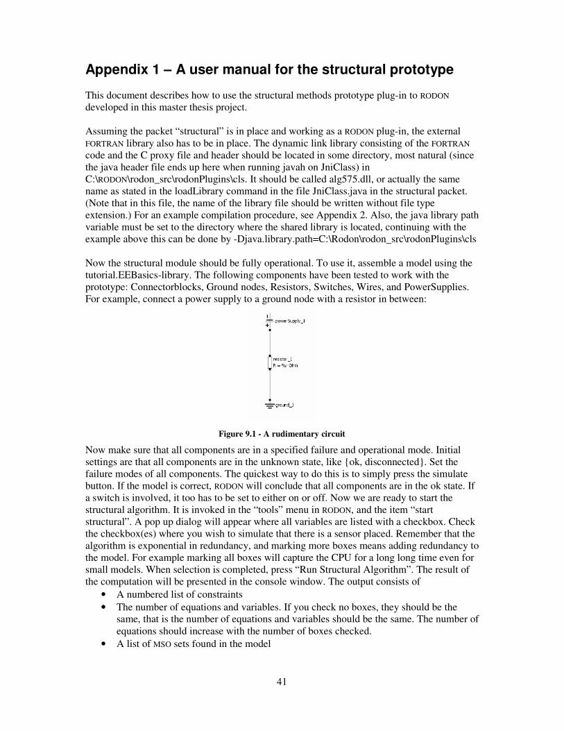
41

Appendix 1 – A user manual for the structural prototype This document describes how to use the structural methods prototype plug-in to RODON developed in this master thesis project. Assuming the packet “structural” is in place and working as a RODON plug-in, the external FORTRAN library also has to be in place. The dynamic link library consisting of the FORTRAN code and the C proxy file and header should be located in some directory, most natural (since the java header file ends up here when running javah on JniClass) in C:\RODON\rodon_src\rodonPlugins\cls. It should be called alg575.dll, or actually the same name as stated in the loadLibrary command in the file JniClass.java in the structural packet. (Note that in this file, the name of the library file should be written without file type extension.) For an example compilation procedure, see Appendix 2. Also, the java library path variable must be set to the directory where the shared library is located, continuing with the example above this can be done by -Djava.library.path=C:\Rodon\rodon_src\rodonPlugins\cls Now the structural module should be fully operational. To use it, assemble a model using the tutorial.EEBasics-library. The following components have been tested to work with the prototype: Connectorblocks, Ground nodes, Resistors, Switches, Wires, and PowerSupplies. For example, connect a power supply to a ground node with a resistor in between:

Figure 9.1 - A rudimentary circuit

Now make sure that all components are in a specified failure and operational mode. Initial settings are that all components are in the unknown state, like {ok, disconnected}. Set the failure modes of all components. The quickest way to do this is to simply press the simulate button. If the model is correct, RODON will conclude that all components are in the ok state. If a switch is involved, it too has to be set to either on or off. Now we are ready to start the structural algorithm. It is invoked in the “tools” menu in RODON, and the item “start structural”. A pop up dialog will appear where all variables are listed with a checkbox. Check the checkbox(es) where you wish to simulate that there is a sensor placed. Remember that the algorithm is exponential in redundancy, and marking more boxes means adding redundancy to the model. For example marking all boxes will capture the CPU for a long long time even for small models. When selection is completed, press “Run Structural Algorithm”. The result of the computation will be presented in the console window. The output consists of

• A numbered list of constraints • The number of equations and variables. If you check no boxes, they should be the

same, that is the number of equations and variables should be the same. The number of equations should increase with the number of boxes checked.

• A list of MSO sets found in the model

42

• The time between clicking “run structural algorithms” on the pop up till the output is sent to console.

43

Appendix 2 – Running Fortran code from java Calling FORTRAN 77 subroutine from java example, using JNI, mingw-gcc/g77 and jdk 1.5 This is a guide on calling a simple subroutine in FORTRAN from java, using JNI. This is done on a windows xp machine using mingw open-source windows-ports of gcc and g77. Java Native Interface (JNI) from jdk 1.5 is also used. Preparations: Write a FORTRAN file (helloWorld.for) containing a subroutine HELLOWORLDFORTRAN: C Hello World subroutine in FORTRAN 77 SUBROUTINE HELLOWORLDFORTRAN() PRINT*, 'HELLO WORLD, BEST REGARDS FROM FORTRAN!' RETURN END 1. Write the java file HelloWorld.java: public class HelloWorld{ public static void main(String[] args) { helloWorld(); } public static native void helloWorld(); static { System.loadLibrary("hello"); } } 2. Compile HelloWorld.java: javac HelloWorld.java 3. Generate C-header: javah Helloworld 4. Implement C-function, (helloProxy.c) and include generated header file: (And add trailing underscore to FORTRAN function call! Also it needs to be lower-case.) #include "HelloWorld.h" JNIEXPORT void JNICALL Java_HelloWorld_helloWorld(JNIEnv *env, jclass c){ helloworldfortran_(); } 5. Compile C-file helloProxy.c to object file helloProxy.o, including some java libraries, and making it a shared object: gcc -I"C:\Program Files\Java\jdk1.5.0_08\include" -I"C:\Program Files\Java\jdk1.5.0_08\include\win32" -c -shared helloProxy.c

44

6. Compile fortran file and at the same time link in the previously produced object file to create the hello.dll: g77 -o hello.dll -shared -Wl,--add-stdcall-alias helloProxy.o HelloWorld.for 7. Run the program! java HelloWorld HELLO WORLD, BEST REGARDS FROM FORTRAN!

45

På svenska Detta dokument hålls tillgängligt på Internet – eller dess framtida ersättare – under en längre tid från publiceringsdatum under förutsättning att inga extra-ordinära omständigheter uppstår.

Tillgång till dokumentet innebär tillstånd för var och en att läsa, ladda ner, skriva ut enstaka kopior för enskilt bruk och att använda det oförändrat för ickekommersiell forskning och för undervisning. Överföring av upphovsrätten vid en senare tidpunkt kan inte upphäva detta tillstånd. All annan användning av dokumentet kräver upphovsmannens medgivande. För att garantera äktheten, säkerheten och tillgängligheten finns det lösningar av teknisk och administrativ art.

Upphovsmannens ideella rätt innefattar rätt att bli nämnd som upphovsman i den omfattning som god sed kräver vid användning av dokumentet på ovan beskrivna sätt samt skydd mot att dokumentet ändras eller presenteras i sådan form eller i sådant sammanhang som är kränkande för upphovsmannens litterära eller konstnärliga anseende eller egenart.

För ytterligare information om Linköping University Electronic Press se förlagets hemsida http://www.ep.liu.se/ In English The publishers will keep this document online on the Internet - or its possible replacement - for a considerable time from the date of publication barring exceptional circumstances.

The online availability of the document implies a permanent permission for anyone to read, to download, to print out single copies for your own use and to use it unchanged for any non-commercial research and educational purpose. Subsequent transfers of copyright cannot revoke this permission. All other uses of the document are conditional on the consent of the copyright owner. The publisher has taken technical and administrative measures to assure authenticity, security and accessibility.

According to intellectual property law the author has the right to be mentioned when his/her work is accessed as described above and to be protected against infringement.

For additional information about the Linköping University Electronic Press and its procedures for publication and for assurance of document integrity, please refer to its WWW home page: http://www.ep.liu.se/

© Oskar Särnholm