WITH ELASTIC MODULUS AND POISSON'S RATIO …

Poisson's Ratio (v) / Stress Curve

Tan Sec

Stress (MPa)160140120100806040200

Poi

sson

's R

atio

(v)

1.0

0.8

0.6

0.4

0.2

0.0

AxialRadial

Stress / Strain Curve

Microstrain1 6001 4001 2001 0008006004002000-200-400

Str

ess

(MP

a)

160

128

96

64

32

UNIAXIAL COMPRESSION TESTWITH ELASTIC MODULUS AND POISSON'S RATIO MEASUREMENTS BY MEANS OF STRAIN GAUGES

Modulus (E) / Stress Curve

Tan Sec

Stress (MPa)160140120100806040200

Mod

ulus

(E

) (G

Pa)

180

160

140

120

100

80

60

40

20

0

2018/11/07 10:40:43

Axial Strain at Failure: 1727 microstrain

% Strength Strength (MPa) E Tan (GPa) E Sec (GPa) v Secv Tan

10

20

30

40

50

60

70

80

90

16.2

32.5

48.7

64.9

81.2

97.4

114

130

146

95.9 97.3 0.270 0.289

96.8 96.2 0.240 0.267

79.3 93.4 0.207 0.246

95.3 91.7 0.276 0.247

93.7 91.8 0.219 0.246

97.4 91.8 0.251 0.241

97.5 92.6 0.250 0.243

97.5 93.2 0.250 0.244

97.5 93.6 0.250 0.245

ROCKLAB230 Albertus Street

La MontagneTel (012) 481-3894Fax (012) 481-3812

P O Box 72928Lynnwood Ridge

0040email: [email protected]

A division of Soillab(PTY) LTD

Reg. No. 71/00112/07

Specimen No: 7743-ucm-02

Peak Strength: 162.3 MPaFailure Load: 345.5 kN

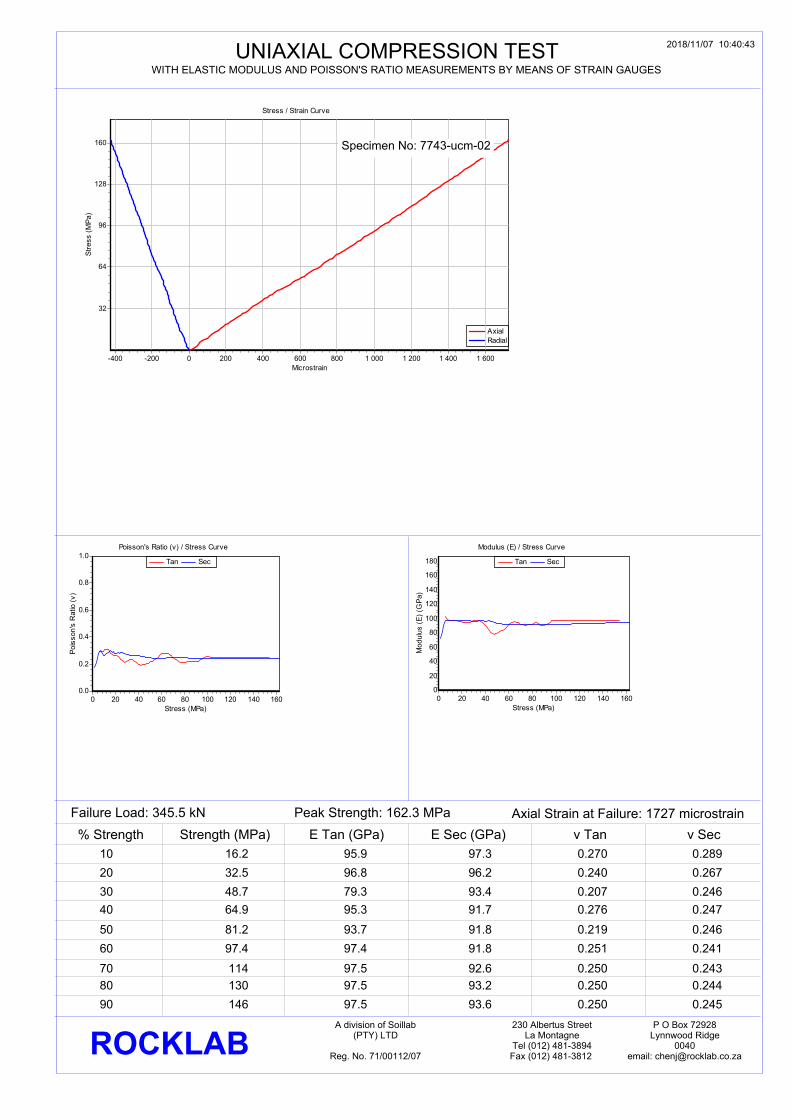
APPENDIX 2

CLASSIFICATION OF ROCK SPECIMEN FAILURE MODE INFLUENCED / NOT INFLUENCED BY DISCONTINUITIES DURING COMPRESSION

TESTING

FAILURE NOT INFLUENCED BY DISCONTINUITIES (INTACT)

DESCRIPTION OF SUB CODES TYPE CODE A B

X SINGLE SLIDING SHEAR FAILURE COMPLETE CONE DEVELOPMENT

Y SPLITTING

FAILURE INFLUENCED BY DISCONTINUITIES

DESCRIPTION OF SUB CODES

A B TYPE CODE

PARTIAL FAILURE ON DISCONTINUITY FAILURE COMPLETELY ON DISCONTINUITY

1 AT 0-10◦ TO AXIS AT 0-10◦ TO AXIS







0 Multiple Discontinuities Multiple Discontinuities

Example: Failure Type3B: Failure completely on a discontinuity with an orientation of

between 21◦and 30◦ to the specimen axis.

AngloGold Ashanti

KAREERAND TSF EXTENSION PROJECT

FEASIBILITY STUDY FOR KAREERAND TSF EXTENSION PROJECT

301-00204/13 Rev 1

October 2, 2019

Deterministic Seismic Hazard Analysis Report

1

DETERMINISTIC SEISMIC HAZARD ANALYSIS

for

Kareerand Tailing Dam, Stilfontein

Submitted to

Knight Piésold (Pty) Ltd. 4 De la Rey Road,

Rivonia | Gauteng | South Africa | 2128 phone: +27 11 806 7111 | fax: +27 11 806 7100

web: http://www.knightpiesold.com

Prepared by

A Kijko Natural Hazard Assessment Consultancy

8 Birch St Clubview ext 2, Centurion 0157

South Africa cell: +27(0)829394002

e-mail: [email protected]

Report No: 2016-17/2 (Rev 2.0)

2

Table of Contents

1. Executive Summary…………………………………………………………………………...3 2. Definition of Terms, Symbols and Abbreviations………….………………………………..5 3. List of Figures………………………………………………………………………………….9 4. Terms of Reference……………………………………………………………………………9 5. Deterministic Seismic Hazard Analysis – Fundamentals………………………………….11

5.1 Assessment of the maximum regional earthquake magnitude, mmax

6. Seismicity of the Selected Area and their Parameters…………………………………..…15 7. Applied Intensity Prediction Equations (IPEs)…………………………………………….19 8. Deterministic Seismic Hazard Analysis for the Kareerand Tailing Dam – Results

8.1 Account of uncertainties: Logic Tree Approach…………………………….……20

9. Newmark-Hall Elastic Response Spectra…………………………………………………..22 10. Conclusions……………………………………………………………………………….....25 11. References…………………………………………………………………………………...26

Appendices Appendix A: Seismicity of area surrounding the Kareerand Tailing Dam in the radius of 50 km.

Appendix B: Results of seismic hazard analysis for the area in vicinity of the KTD in terms of seismic event magnitude (tabulated values of mean activity rate, return periods and probability of exceedance in 1, 5, 10 and 25 years). Appendix C: Attenuation of Vertical Peak Acceleration (by N. A. Abrahamson and J.J. Litehiser) Appendix D: “Introduction to Probabilistic Seismic Hazard Analysis” (Extended version of contribution by A. Kijko, Encyclopedia of Solid Earth Geophysics, Harsh Gupta (Ed.), Springer, 2011 Compiled by:

………………………….....……………………… Prof. A. Kijko 12 November 2017 (Rev 2.0) NHAC

3

1. Executive Summary

A Deterministic Seismic Hazard Analysis (DSHA) has been performed for the site of the Kareerand Tailing Dam (KTD), Stilfontein. All known seismic events with magnitude MW 3.0 located within a radius of 50 km from the site were used in the assessment.

The study consists of the development of a particular seismic scenario upon which a seismic hazard evaluation is based (Reiter, 1990; Kramer, 1996). The scenario consists of the postulated occurrence of seismic event of a specified size occurring in a specified area. The DSHA for the KTD includes the following investigations:

Compilation of a seismic events catalogue and selection of seismic event within a 50 km radius of the dam.

Identification of seismic event capable of producing significant ground motion (peak

ground acceleration) at the site of the dam.

Assessment of the annual probability of exceeding the specified value of seismic event magnitude and its return period. At the same time the analysis provides assessment of the worst-case scenario, i.e. occurrence of seismic event with the maximum possible magnitude in vicinity of the dam.

A selection of the controlling seismic event, i.e. the event that is expected to generate the

strongest level of shaking, in our case, expressed in terms of PGA. The controlling event is described in terms of its magnitude and distance from the dam site. In this report the controlling event is determined as event of MW magnitude 5.63 0.11 located at the epicenter of 9th March 2005 Stilfontein event. The MW = 5.63 0.11 is considered as maximum possible, mine related seismic event magnitude, characteristic to the area.

Selection of most adequate Modified Mercalli intensity (MMI) prediction equation (IPE). All calculations are repeated three times, each for a different IPE:

(1) Stable Continental Regions – Modified. The IPE was originally designed as intensity prediction equation for stable continental regions and modified for South African conditions (Midzi et al., 2015).

(2) Regional. The IPE developed exclusively for the Klerksdorp gold mining area (Hattingh et al., 2006).

(3) Stable Continental Regions – Global. The IPE developed for European stable continental region. The IPE provides the lowest residuals for near-source (< 50 km) intensity observations in stable continental regions (Bakun and Scotti, 2006).

4

Conversion of estimated MMI into PGA. Since it is unclear which conversion formula of MMI into PGA are best suited for the region, two classic conversion formulas were applied (Ambraseys, 1974, and Trifunac and Brady, 1975) and the final PGA was determined by application of the logic tree formalism.

The development of a Newmark and Hall Elastic Acceleration Response Spectra for 5% damping anchored at PGA predicted at the dam site by the occurrence of the controlling seismic event.

The results of the DSHA are given in terms of largest expected horizontal value of the peak ground acceleration calculated by application of logic tree formalism. The predicted largest horizontal PGA at the site of dam is 0.152 0.098 g. Lists of all seismic events used in the study are given in Appendix A. Appendix B provides results of seismic hazard analysis for area in vicinity of the KTD in terms of seismic event magnitude (tabulated values of mean activity rate, return periods and probability of exceedance in 1, 5, 10 and 25 years). Appendix C provides study by N.A. Abrahamson and J.J. Litehiser on the attenuation of the vertical peak acceleration. Finally, the Appendix D provides the fundamentals of a deterministic and probabilistic seismic hazard analysis.

5

2. Definition of Terms, Symbols and Abbreviations Acceleration The rate of change of particle velocity per unit time.

Commonly expressed as a fraction or percentage of the acceleration due to gravity (g), where g = 9.81 m/s2.

Acceleration Response Spectra (ARS) Spectral acceleration is the movement experienced by a structure during an earthquake.

Annual Probability of Exceedance The probability that a given level of seismic hazard (typically some measure of ground motions, e.g., seismic magnitude or intensity), or seismic risk (typically economic loss or casualties)

Area-specific mean seismic activity rate (A) Mean rate of seismicity for the whole selection area in the vicinity of the site for which the PSHA is performed.

Attenuation A decrease in seismic-signal amplitude as waves propagate from the seismic source. Attenuation is caused by geometric spreading of seismic-wave energy and by the absorption and scattering of seismic energy in different earth materials.

Attenuation law - ground motion prediction equation (GMPE)

A mathematical expression that relates a ground motion parameter, such as the peak ground acceleration, to the source and propagation path parameters of an earthquake such as the magnitude, source-to-site distance, fault type, etc. Its coefficients are usually derived from statistical analysis of earthquake records. It is a common engineering term known as ground motion prediction equation (GMPE).

b-value (b) A coefficient in the frequency-magnitude relation, log N(m) = a – bm, obtained by Gutenberg and Richter (1941; 1949), where m is the earthquake magnitude and N(m) is the number of earthquakes with magnitude greater than or equal to m. Estimated b-values for most seismic sources fall between 0,6 and 1,2.

Capable (active) fault

A mapped fault that is deemed a possible site for a future earthquake with magnitude greater than some specified threshold.

Catalogue (seismic events) A chronological listing of earthquakes. Early catalogues were purely descriptive, i.e., they gave the date of each earthquake and some description of its effects. Modern catalogues are usually quantitative, i.e., earthquakes are listed as a set of numerical parameters describing origin time, hypocenter location, magnitude, focal mechanism, moment tensor, etc.

Design Earthquake The postulated earthquake (commonly including a specification of the ground motion at a site) that is used for evaluating the earthquake resistance of a particular structure.

Elastic design spectrum (or spectra) The specification of the required strength or capacity of the structure plotted as a function of the natural period or frequency of the structure appropriate to earthquake response at the required level. Design spectra are often composed of straight line segments (Newmark and Hall, 1982) and/or

6

simple curves, for example, as in most building codes, but they can also be constructed from statistics of response spectra of a suite of ground motions appropriate to the design earthquake(s). To be implemented, the requirements of a design spectrum are associated with allowable levels of stresses, ductilities, displacements or other measures of response.

Earthquake Ground shaking and radiated seismic energy caused most commonly by sudden slip on a fault, volcanic or magmatic activity, or other sudden stress changes in the Earth.

Epicentre The epicentre is the point on the earth's surface vertically above the hypocenter (or focus).

Epicentral distance () Distance from the site to the epicentre of an earthquake.

Fault A fracture or fracture zone in the Earth along which the two sides have been displaced relative to one another parallel to the fracture. The accumulated displacement may range from a fraction of a meter to many kilometres. The type of fault is specified according to the direction of this slip. Sudden movement along a fault produces earthquakes. Slow movement produces a seismic creep.

Focal depth (h) Focal depth is the vertical distance between the hypocentre and epicentre.

Frequency

The number of cycles of a periodic motion (such as the ground shaking up and down or back and forth during an earthquake) per unit time; the reciprocal of period. Hertz (Hz), the unit of frequency, is equal to the number of cycles per second.

Ground motion

The movement of the earth's surface from earthquakes or explosions. Ground motion is produced by waves that are generated by sudden slip on a fault or sudden pressure at the explosive source and travel through the earth and along its surface.

Ground motion parameter A parameter characterising ground motion, such as peak acceleration, peak velocity, and peak displacement (peak parameters) or ordinates of response spectra and Fourier spectra (spectral parameters).

Heterogeneity A medium is heterogeneous when its physical properties change along the space coordinates. A critical parameter affecting seismic phenomena is the scale of heterogeneities as compared with the seismic wavelengths. For a relatively large wavelength, for example, an intrinsically isotropic medium with oriented heterogeneities may behave as a homogeneous anisotropic medium.

Hypocenter The hypocenter is the point within the earth where an earthquake rupture starts. The epicentre is the point directly above it at the surface of the Earth. Also commonly termed the focus.

Hypocentral distance (r)

Distance from the site to the hypocenter of an earthquake.

Induced earthquake An earthquake that results from changes in crustal stress

7

and/or strength due to man-made sources (e.g., underground mining and filling of a water reservoir), or natural sources (e.g., the fault slip of a major earthquake). As defined less rigorously, “induced” is used interchangeably with “triggered” and applies to any earthquake associated with a stress change, large or small.

Local Magnitude (ML) A magnitude scale introduced by Richter (1935) for earthquakes in southern California. ML was originally defined as the logarithm of the maximum amplitude of seismic waves on a seismogram written by the Wood-Anderson seismograph (Anderson and Wood, 1925) at a distance of 100 km from the epicentre. In practice, measurements are reduced to the standard distance of 100 km by a calibrating function established empirically. Because Wood-Anderson seismographs have been out of use since the 1970s, ML is now computed with simulated Wood-Anderson records or by some more practical methods.

Magnitude In seismology, a quantity intended to measure the size of earthquake and is independent of the place of observation. Richter magnitude or local magnitude (ML) was originally defined in Richter (1935) as the logarithm of the maximum amplitude in micrometres of seismic waves in a seismogram written by a standard Wood-Anderson seismograph at a distance of 100 km from the epicentre. Empirical tables were constructed to reduce measurements to the standard distance of 100 km, and the zero of the scale was fixed arbitrarily to fit the smallest earthquake then recorded. The concept was extended later to construct magnitude scales based on other data, resulting in many types of magnitudes, such as body-wave magnitude (mb), surface-wave magnitude (MS), and moment magnitude (MW). In some cases, magnitudes are estimated from seismic intensity data, tsunami data, or duration of coda waves. The word “magnitude” or the symbol M, without a subscript, is sometimes used when the specific type of magnitude is clear from the context, or is not really important.

Maximum Regional Earthquake Magnitude (mmax)

Upper limit of magnitude for a given seismogenic zone or entire region. Often also referred to as the maximum credible earthquake (MCE).

Oscillator In earthquake engineering, an oscillator is an idealised mass-spring system used as a model of the response of a structure to earthquake ground motion. A seismograph is also an oscillator of this type

Peak Ground Acceleration (PGA) The maximum acceleration amplitude measured (or expected) of an earthquake.

Probabilistic Seismic Hazard Analysis (PSHA)

Available information on earthquake sources in a given region is combined with theoretical and empirical relations among earthquake magnitude, distance from the source and local site conditions to evaluate the exceedance probability of a certain ground motion parameter, such as the peak acceleration, at a given site during a prescribed period.

Response spectrum The response of the structure to a specified acceleration time series of a set of single-degree-of-freedom oscillators with chosen levels of viscous damping, plotted as a function of the undamped natural period or undamped natural frequency

8

of the system. The response spectrum is used for the prediction of the earthquake response of buildings or other structures.

Seismic Hazard Any physical phenomena associated with an earthquake (e.g., ground motion, ground failure, liquefaction, and tsunami) and their effects on land use, man-made structure and socio-economic systems that have the potential to produce a loss. It is also used without regard to a loss to indicate the probable level of ground shaking occurring at a given point within a certain period of time.

Seismic Wave

A general term for waves generated by earthquakes or explosions. There are many types of seismic waves. The principle ones are body waves, surface waves, and coda waves.

Seismic zone An area of seismicity probably sharing a common cause.

Seismogenic Capable of generating earthquakes.

Site-specific mean activity rate (λ) Mean activity rate of the selected ground motion parameter experienced at the site.

Strong ground motion A ground motion having the potential to cause significant risk to a structure's architectural or structural components, or to its contents. One common practical designation of strong ground motion is a peak ground acceleration (PGA) of 0.05g or larger.

IPE Intensity prediction equation

9

3. List of Figures and Tables 3.1. List of Figures Figure 6.1 Distribution of all known seismic events with moment magnitude MW 3.0 and stronger within 50 km radius of the Kareerand Tailing Dam. The dam location is shown as a blue square. Figure 6.2 The annual probability of exceeding the specified value of seismic event magnitude for the area within 50 km from the KTD site. The red curve shows the mean probability, while the two blue curves indicate the mean probability plus or minus the standard deviation. Figure 6.3 The mean return periods for seismic events occurring within the area of 50 km from the KTD site.

Figure 6.4 Probability of exceedance of specified value of magnitude within time interval 5, 10 and 25 years for the area within 50 km from the KTD site. Figure 9.1 Newmark-Hall elastic design spectra (horizontal) anchored at the PGA resulting from application of logic tree procedure. 3.2. List of Tables Table 6-1 Division of the catalogue used in the analysis. mmin = Level of Completeness; SE = standard error of seismic event magnitude determination.

Table 8-1 Expected values of MMI and PGA at the site of seismic event of magnitude MW = 5.63 located at the epicenter of the Stilfontein event of the 9th March 2005.

4. Terms of Reference

Due extremely high seismic activity in vicinity of the Kareerand Tailing Storage Facility (9th March 2005, Stilfontein seismic event with magnitude 5.3 and Orkney event 5th, August 2014, magnitude 5.4), the Natural Hazard Assessment Consultancy (NHAC) was requested by Mr Duncan Grant-Stuart, Technical Consultant Knight Piésold (Pty) Ltd (E: [email protected]), to provide desk study of a deterministic seismic hazard analysis (DSHA) for the site of KTD. No geological investigations were required at this stage. In general, the hazardous effects of earthquakes can be divided into three categories:

1. Those resulting directly from a certain level of ground shaking.

10

2. Those at the site resulting from surface faulting or deformations. 3. Those triggered or activated by a certain level of ground shaking, such as the generation

of a tsunami or landslide.

This study only covers category one and the case of deterministic seismic hazard analysis (DSHA) and is limited to the following investigations:

Compilation of a seismic events catalogue within a 50 km radius of the dam.

Identification of seismic event capable of producing significant ground motion (peak ground acceleration) at the site of the dam.

Assessment of the annual probability of exceeding the specified value of seismic event magnitude and its return period. At the same time the analysis provides assessment of the worst-case scenario, i.e. occurrence of seismic event with the maximum possible magnitude in vicinity of the dam.

Assessment of effect of the controlling seismic event, i.e. the event that is expected to generate the strongest level of shaking, in our case, expressed in terms of peak ground acceleration (PGA). The controlling event is described in terms of its magnitude and distance from the dam site.

Selection of most adequate Modified Mercalli intensity (MMI) prediction equation (IPE).

Conversion of estimated MMI into PGA.

The development of a Newmark and Hall Elastic Acceleration Response Spectra for 5% damping anchored at PGA predicted at the dam site by the occurrence of the controlling seismic event.

The results of the DSHA are given in terms of largest expected horizontal peak ground acceleration calculated by application of logic tree formalism. Lists of all seismic events used in the study are given in Appendix A. Appendix B provides results of seismic hazard analysis for the area in vicinity of KTD in terms of seismic event magnitude (tabulated values of mean activity rate, return periods and probability of exceedance in 1, 5, 10 and 25 years). Appendix C provides work by N.A. Abrahamson and J.J. Litehiser on the attenuation of the vertical peak acceleration. Finally, the Appendix D provides the fundamentals of a deterministic and probabilistic seismic hazard analysis.

11

5. Deterministic Seismic Hazard Analysis – Fundamentals. Deterministic seismic hazard analysis (DSHA) involves the development of a particular seismic scenario, according to which expected damages (losses) can be estimated. It provides a framework for evaluation of the worst-case damages. However, it provides no information on the likelihood of occurrence of such damages. Deterministic seismic hazard analysis, involves subjective assumptions, particularly regarding earthquake potential as described by the area characteristic, maximum possible earthquake magnitude (Reiter, 1990). The earthquake magnitudes referred to are moment, Richter scale magnitudes (Lay and Wallace, 1995). These magnitudes are a measure of the total energy released at the hypocentre of the earthquake with the hypocentre defined as the underground, initial point of origin of an earthquake compared to the epicentre which is the point on the surface of the earth directly above the hypocentre (Lay and Wallace, 1995). The increase of earthquake magnitude by one unit corresponds with the increase in energy released by an earthquake by approximately 30 times. The strength of a seismic event at a given site is measured in terms of the Modified Mercalli intensity (MMI) scale, a subjective scale based on resultant structural damage to buildings. The MMI felt at a specific location varies according to the distance from the hypocentre of the earthquake to the location. There are two common assumptions made in modelling of seismic event occurrence. Firstly, the number of main seismic events in the time interval , follows a Poisson distribution with parameter , where is the frequency (annual mean activity rate) of earthquake occurrence. Secondly, the earthquake magnitudes follow the Gutenberg-Richter relation (Gutenberg and Richter, 1956),

ln (1) where is the number of earthquakes, is the earthquake magnitude, is a constant measuring the level of seismicity and is a constant which characterises the ratio between small events to large ones. The Gutenberg-Richter relation is the logarithm-frequency-magnitude relation where the plot of the logarithm of the number of earthquakes against the magnitude is linear. If the magnitudes of seismic events are assumed to be independent, identically distributed random variables, where the frequency-magnitude Gutenberg-Richter relation (1) can be expressed in terms of distribution functions as (Page, 1968)

0 exp

1 exp

0

(2)

12

and

0 1 exp

1 exp,

1

(3)

where and are respectively the probability density function (PDF) and cumulative distribution function (CDF) of magnitude , where , ln 10 and is the -parameter of the Gutenberg-Richter relation (1). The maximum likelihood estimator of the

-value, denoted as , can be obtained from solution of equation (Page, 1968)

1 exp1 exp

, (4)

where is the sample mean magnitude. The value of can be obtained only by recursive

solutions. The approximate standard error of , denoted as , is (Aki, 1965)

√ (5)

such that is number of earthquakes with magnitudes greater or equal to . It is also assumed that earthquakes with magnitudes larger or equal to that occurred in a specified time interval are recorded. The time span for the seismic event catalogue is measured in years. The earthquake magnitudes are assumed to be random variables with the PDF

and CDF . The magnitudes are denoted as 1,2, … , and ordered such that is the maximum observed earthquake and ⋯ . An integral part of any DSHA is the selection of an area-characteristic intensity prediction equation (IPE) and the calculation of the expected ground motion at the site as generated by the control earthquake. An MMI IPE is a relationship that translates the maximum (focal) MMI at the epicentre ( ) into MMI at the site. The most often used the IPE relation has the following form

ln , (6) where , , are empirical coefficients, is the chosen epicentral or hypocentral distance, is MMI at the site and is the maximum (focal) MMI at the epicentre. The numerical values of

13

coefficients , , are different for different regions and are usually estimated from MMI distribution maps of the region. The empirical relation between earthquake magnitude and MMI at the epicentre , is given by (Richter, 1958):

32

1. (7)

5.1 Assessment of the Maximum Regional Earthquake magnitude, mmax The maximum possible earthquake magnitude is defined as the upper limit of earthquake magnitude for a given region. Also, synonymous with the upper limit of earthquake magnitude is the magnitude of the largest possible earthquake for a given region (EERI Committee, 1984).

Although value of maxm is one of the most important parameter in seismic hazard analysis, it is

astonishing how little has been done in developing appropriate techniques for its estimation.

Presently, there is no universally accepted technique for estimating the value of maxm , however,

the current procedures for maxm can be divided into two main categories: deterministic and

probabilistic. A presentation and discussion of deterministic techniques for the assessment of

maxm can be found in e.g. Wells and Coppersmith (1994); Wheeler (2009) and Mueller (2010).

The selection of the applied probabilistic procedure depends on the assumptions about the statistical distribution model and/or the information available about past seismicity. Taking into account that in the case of seismic hazard assessment for the KTD, the available data are extremely uncertain, the most appropriate is the nonparametric procedure which is applicable in case of uncertainty of both, the data and the recurrence model (Kijko and Singh, 2011). Let us assume that the form of the magnitude distribution is not known and we wish to estimate the right end point of the distribution, viz. the maximum earthquake magnitude mmax. One of the methods to solve this problem is to apply the classic Quenouille (1956) technique of successive bias reduction, modified to fit the factorial series rather than the power series in 1/n. Robson and Whitlock (1964) showed that, under very general conditions, and when the data are arranged in ascending order of magnitude, viz. ⋯ , Quenouille’s approach leads to the following rule in estimation of mmax

)(ˆ 1maxmaxmax nobsobs mmmm (8)

14

Equation (8) was first derived by Robson and Whitlock (1964), and is often called the Robson and Whitlock (R-W) estimator. It can be shown that the above estimator is mean-unbiased to order n-2

and asymptotically median-unbiased.

The simplicity of the (8) makes it very attractive. It can be applied in cases of limited and/or doubtful seismic data, when quick results, without going into sophisticated analysis, is required. Unfortunately, the reduction of bias of the R-W estimator can be achieved only at the expense of a high value of its mean squared error. In fact, Robson and Whitlock (1964) derived a general formula for an unbiased estimator of truncation point,

k

jjn

j mj

km

0max 1

1)1(ˆ

, (9)

where k = 1,…, n-1. Regrettably, this formula does not provide a guarantee that the estimated magnitude is equal to, or exceeds, the observed maximum magnitude . The approximate variance of the R-W estimator of mmax for the frequency-magnitude Gutenberg-Richter distribution is of the form

2

1max2

max )(5)ˆ( nobs

M mmmVAR , (10)

where M denotes standard error in the determination of the two largest observed magnitudes obsmmax and 1nm .

In their seminal work Robson and Whitlock (1964) also derived a formula for an approximate

)%1(100 upper confidence limit for mmax, which is given as

1)(

1Pr 1maxmaxmax n

obsobs mmmm , (11)

The nonparametric estimator (8) is very useful. The great attraction of the non-parametric approach is that it does not require specifying the functional form for the magnitude distribution. Therefore, by its nature, it is able to deal with cases with empirical distributions of any complexity: distributions which considerably violate log-linearity (1) or/and multimodal distributions, which are so characteristic for mine related seismicity (Gibowicz and Kijko, 1994). The drawback of the Robson-Whitlock estimator (8) is that it formally require knowledge of all

15

events with magnitude above the specified level of completeness mmin, though, in practice, this can reduce to the knowledge of a few of the largest events.

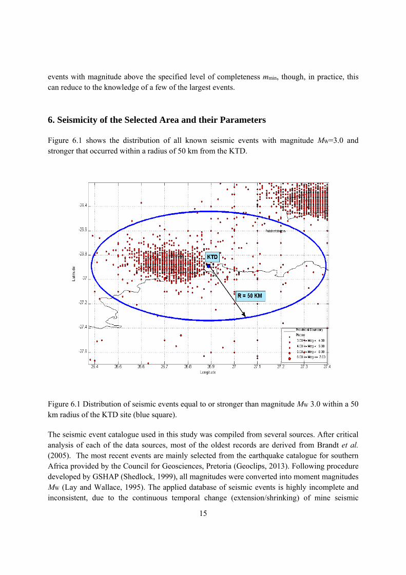
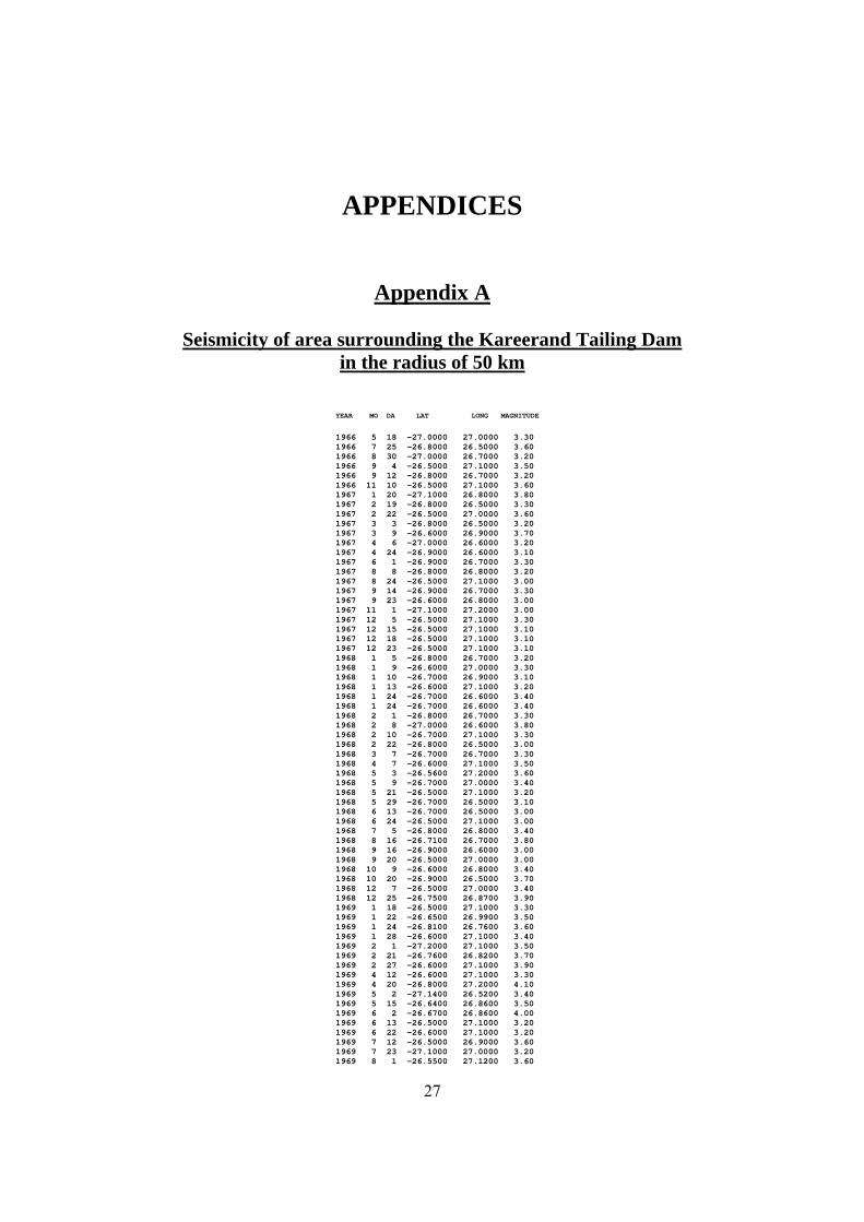
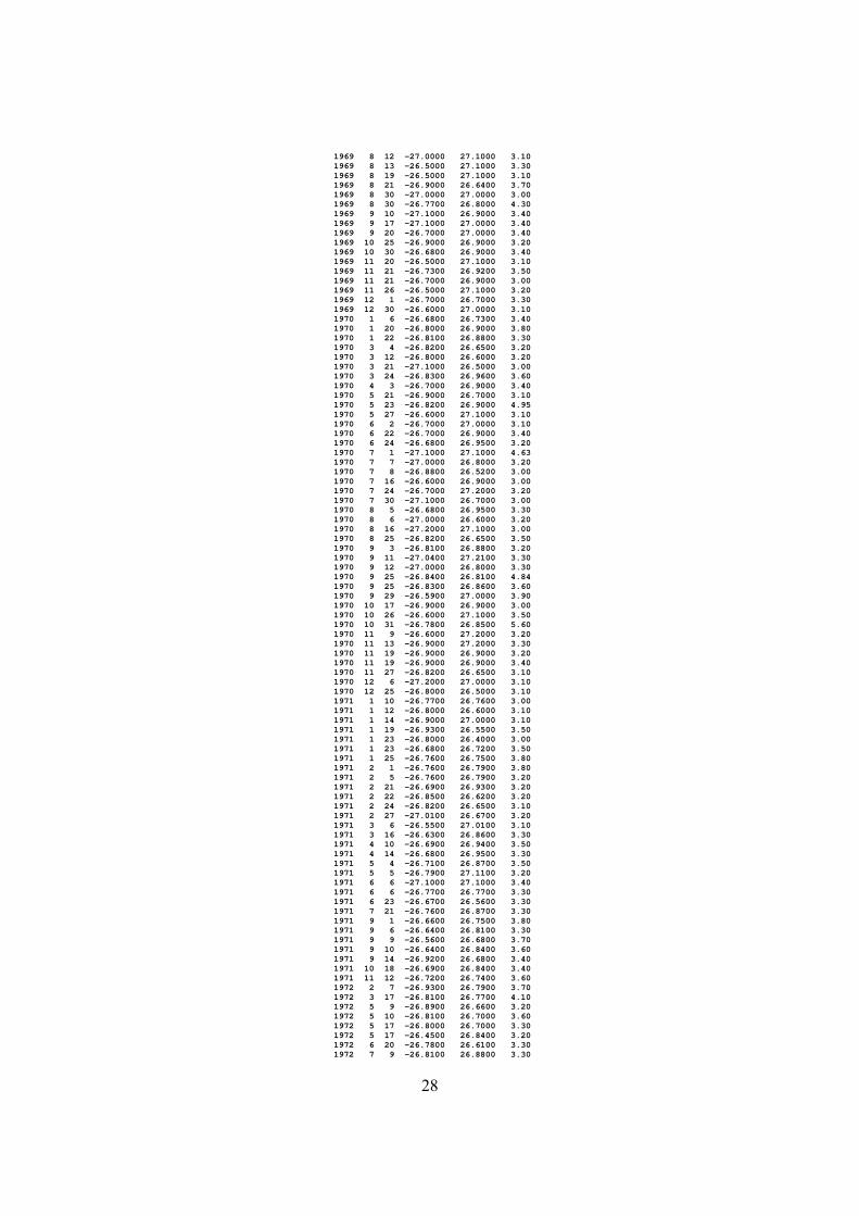
6. Seismicity of the Selected Area and their Parameters Figure 6.1 shows the distribution of all known seismic events with magnitude MW=3.0 and stronger that occurred within a radius of 50 km from the KTD.

Figure 6.1 Distribution of seismic events equal to or stronger than magnitude MW 3.0 within a 50 km radius of the KTD site (blue square).

The seismic event catalogue used in this study was compiled from several sources. After critical analysis of each of the data sources, most of the oldest records are derived from Brandt et al. (2005). The most recent events are mainly selected from the earthquake catalogue for southern Africa provided by the Council for Geosciences, Pretoria (Geoclips, 2013). Following procedure developed by GSHAP (Shedlock, 1999), all magnitudes were converted into moment magnitudes MW (Lay and Wallace, 1995). The applied database of seismic events is highly incomplete and inconsistent, due to the continuous temporal change (extension/shrinking) of mine seismic

16

networks, adjustment of processing software, mixture of different databases, different conventions of magnitude determination and different procedures used to convert different magnitude scales into unified moment magnitude MW. The list of seismic events used in this study, from a radius of 50 km from the KTD is given in Appendix A.

The catalogue used in the analysis spans a period of ca. 50 years; from May 1966 to February 2016. The catalogue is divided into an incomplete (largest events only) and complete part, (Table 6-1).

Table 6-1 Division of the catalogue used in the analysis. mmin = Level of Completeness; SE = standard error of seismic event magnitude determination.

Type of catalogue Time Span mmin SE Incomplete – largest events 1966/05/01 – 1971/04/30 - 0.25

Complete 1971/05/01 – 2015/02/07 3.5 0.2

The recurrence parameters describing area-characteristic seismic hazard, the mean activity rate , b-value of Gutenberg-Richter were calculated according to the maximum likelihood procedure (Kijko and Sellevoll, 1989; 1992; Kijko et al., 2016; and Kijko (2004). The procedure accounts for incompleteness of seismic event catalogues, uncertainty of earthquake magnitudes and uncertainty of applied earthquake recurrence model. The area-characteristic maximum possible earthquake magnitude mmax were calculated according to Robson and Whitlock (1964), equation (8). The earthquake magnitude recurrence curve, H(m), known as the hazard curve, is defined as the probability of a given value of magnitude, m, being exceeded at least once during a specified time interval t. Such a probability can be written as

mFttmH M 1exp)|( , (12)

where FM(m) denotes the cumulative distribution function of seismic event magnitude (equation 3). Based on seismic events recorded in vicinity of 50 km from the KTD site, the estimated

maximum possible seismic event magnitude = 5.630.11, the Gutenberg-Richter

parameter b̂ = 0.89 0.04 and the mean activity rate = 9.3 1.7 [event-s/year], for mmin = 3.5. The seismic hazard is specified for earthquake magnitudes within the range of 3.5 to 5.6. For

each magnitude the calculated mean activity rate ̂ , return period, and probabilities of exceedance in 1, 5, 10 and 25 years are listed in Appendix D. For instance, in the area within

17

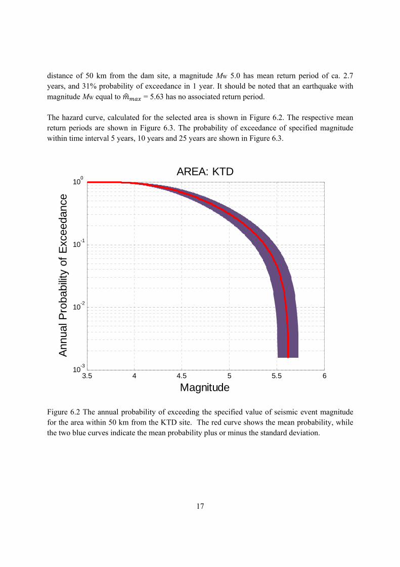
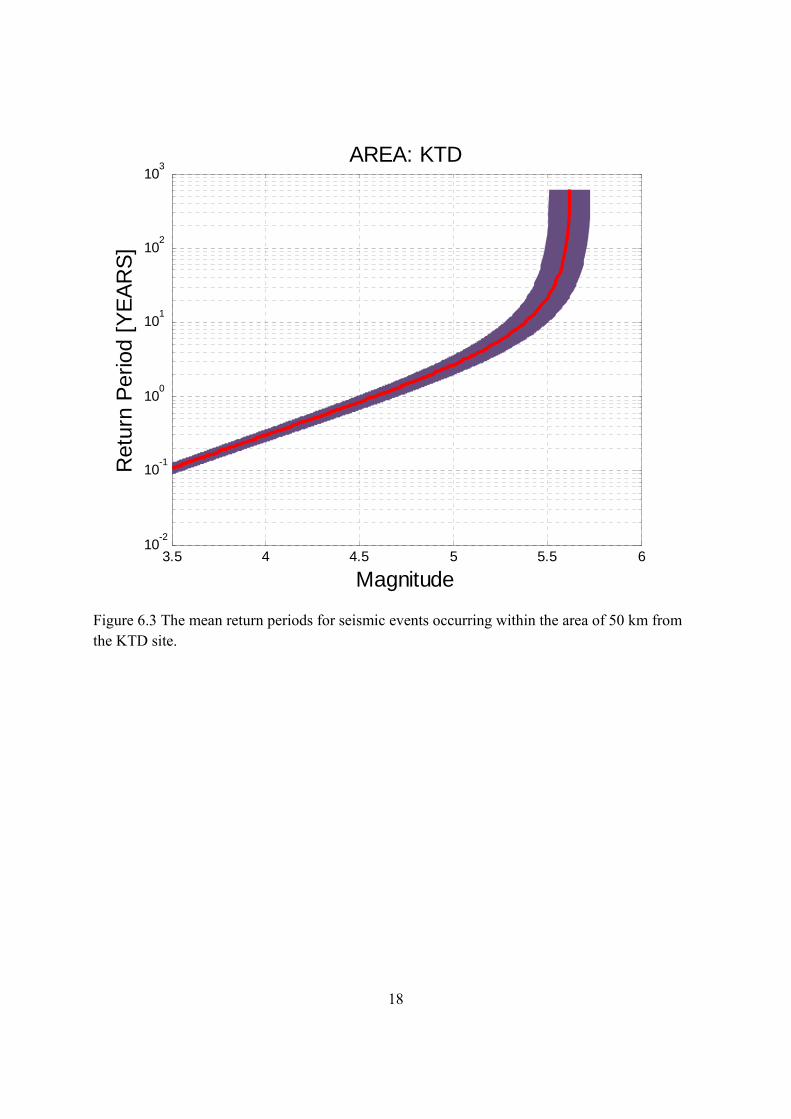
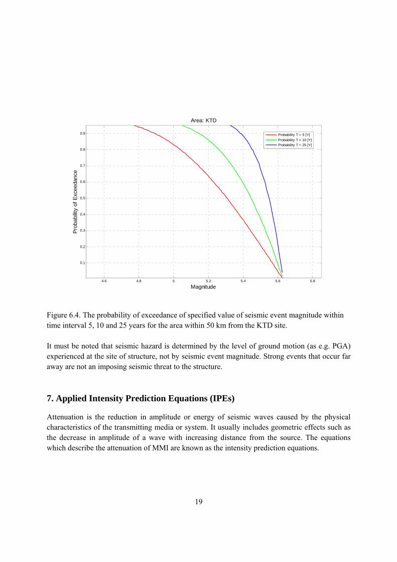
distance of 50 km from the dam site, a magnitude MW 5.0 has mean return period of ca. 2.7 years, and 31% probability of exceedance in 1 year. It should be noted that an earthquake with magnitude MW equal to = 5.63 has no associated return period. The hazard curve, calculated for the selected area is shown in Figure 6.2. The respective mean return periods are shown in Figure 6.3. The probability of exceedance of specified magnitude within time interval 5 years, 10 years and 25 years are shown in Figure 6.3.

Figure 6.2 The annual probability of exceeding the specified value of seismic event magnitude for the area within 50 km from the KTD site. The red curve shows the mean probability, while the two blue curves indicate the mean probability plus or minus the standard deviation.

3.5 4 4.5 5 5.5 610

-3

10-2

10-1

100

AREA: KTD

Magnitude

Annual P

robabili

ty o

f E

xceedance

18

Figure 6.3 The mean return periods for seismic events occurring within the area of 50 km from the KTD site.

3.5 4 4.5 5 5.5 610

-2

10-1

100

101

102

103

AREA: KTD

Magnitude

Retu

rn P

eriod [

YE

AR

S]

19

Figure 6.4. The probability of exceedance of specified value of seismic event magnitude within time interval 5, 10 and 25 years for the area within 50 km from the KTD site. It must be noted that seismic hazard is determined by the level of ground motion (as e.g. PGA) experienced at the site of structure, not by seismic event magnitude. Strong events that occur far away are not an imposing seismic threat to the structure.

7. Applied Intensity Prediction Equations (IPEs) Attenuation is the reduction in amplitude or energy of seismic waves caused by the physical characteristics of the transmitting media or system. It usually includes geometric effects such as the decrease in amplitude of a wave with increasing distance from the source. The equations which describe the attenuation of MMI are known as the intensity prediction equations.

4.6 4.8 5 5.2 5.4 5.6 5.8

0.1

0.2

0.3

0.4

0.5

0.6

0.7

0.8

0.9

Magnitude

Pro

babili

ty o

f E

xceedance

Area: KTD

Probability T = 5 [Y]



20

In this report three intensity prediction equations were used: the Modified Stable Continental Region (SCR), Regional and Global SCR. The SCR - Modified IPE has a form

4.08 1.27 ∙ 3.37 ∙ log ∆ , (13)

where MW denotes moment magnitude and ∆ is epicentral distance in km. Equation (13) has its origin in the IPE derived for stable continental regions and modified for South African conditions (Midzi et al., 2015). The IPE Regional has a form:

0.34 0.324 ∙ ln ∆ 0.0479 ∙ ∆, (14) where MM intensity in epicentre and seismic event magnitude is given by Richter’s (Richter, 1958) empirical relation (7). The IPE was developed exclusively for the Klerksdorp gold mining area (Hattingh et al., 2006). Finally, the IPE SCR - Global,

4.48 1.27 ∙ 3.37 ∙ log , (15) where R denotes hypocentral distance. The IPE was developed for world-wide stable continental regions. The equation provides the lowest residuals of the MMI for small epicentral distances, not exceeded 50 km (Bakun and Scotti, 2006). Moreover, when examining the magnitude dependence, tests show that mostly, it is applicable for only small to moderate-magnitude events, say 4.5 ≤ MW ≤ 5.5. All three applied IPE predict intensities with accuracy close to one unit of MMI.

8. Deterministic Seismic Hazard Analysis for the Kareerand Tailing Dam -

Results

Following our approach, the DSHA requires the development of a particular seismic scenario, which includes the specification of an event capable of producing the strongest level of shaking.

In this report it is assumed that the maximum expected ground motion can be generated by a hypothetical seismic event situated at the epicenter of the 9th March 2005, Stilfontein event, with

magnitude equal to estimated = 5.630.11, located ca. 14.9 km from the dam. The area-characteristic, maximum possible seismic event magnitude was calculate according to procedure by Robson-Whitlock, as described by Kijko and Singh (2011).

21

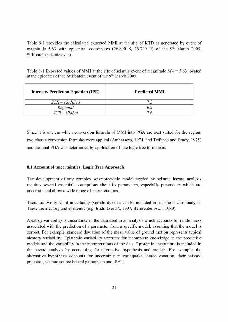
Table 8-1 provides the calculated expected MMI at the site of KTD as generated by event of magnitude 5.63 with epicentral coordinates (26.890 S, 26.740 E) of the 9th March 2005, Stilfontein seismic event. Table 8-1 Expected values of MMI at the site of seismic event of magnitude MW = 5.63 located at the epicenter of the Stilfontein event of the 9th March 2005.

Intensity Prediction Equation (IPE)

Predicted MMI

SCR – Modified 7.3 Regional 6.2

SCR – Global 7.6

Since it is unclear which conversion formula of MMI into PGA are best suited for the region,

two classic conversion formulas were applied (Ambraseys, 1974, and Trifunac and Brady, 1975)

and the final PGA was determined by application of the logic tree formalism.

8.1 Account of uncertainties: Logic Tree Approach

The development of any complex seismotectonic model needed by seismic hazard analysis requires several essential assumptions about its parameters, especially parameters which are uncertain and allow a wide range of interpretations. There are two types of uncertainty (variability) that can be included in seismic hazard analysis. These are aleatory and epistemic (e.g. Budnitz et al., 1997; Bernreuter et al., 1989). Aleatory variability is uncertainty in the data used in an analysis which accounts for randomness associated with the prediction of a parameter from a specific model, assuming that the model is correct. For example, standard deviation of the mean value of ground motion represents typical aleatory variability. Epistemic variability accounts for incomplete knowledge in the predictive models and the variability in the interpretations of the data. Epistemic uncertainty is included in the hazard analysis by accounting for alternative hypothesis and models. For example, the alternative hypothesis accounts for uncertainty in earthquake source zonation, their seismic potential, seismic source hazard parameters and IPE’s.

22

The lack of one, reliable intensity prediction equation and information about the seismic capability of tectonic faults in vicinity of the KTD are the main sources of uncertainty in this DSHA assessment.

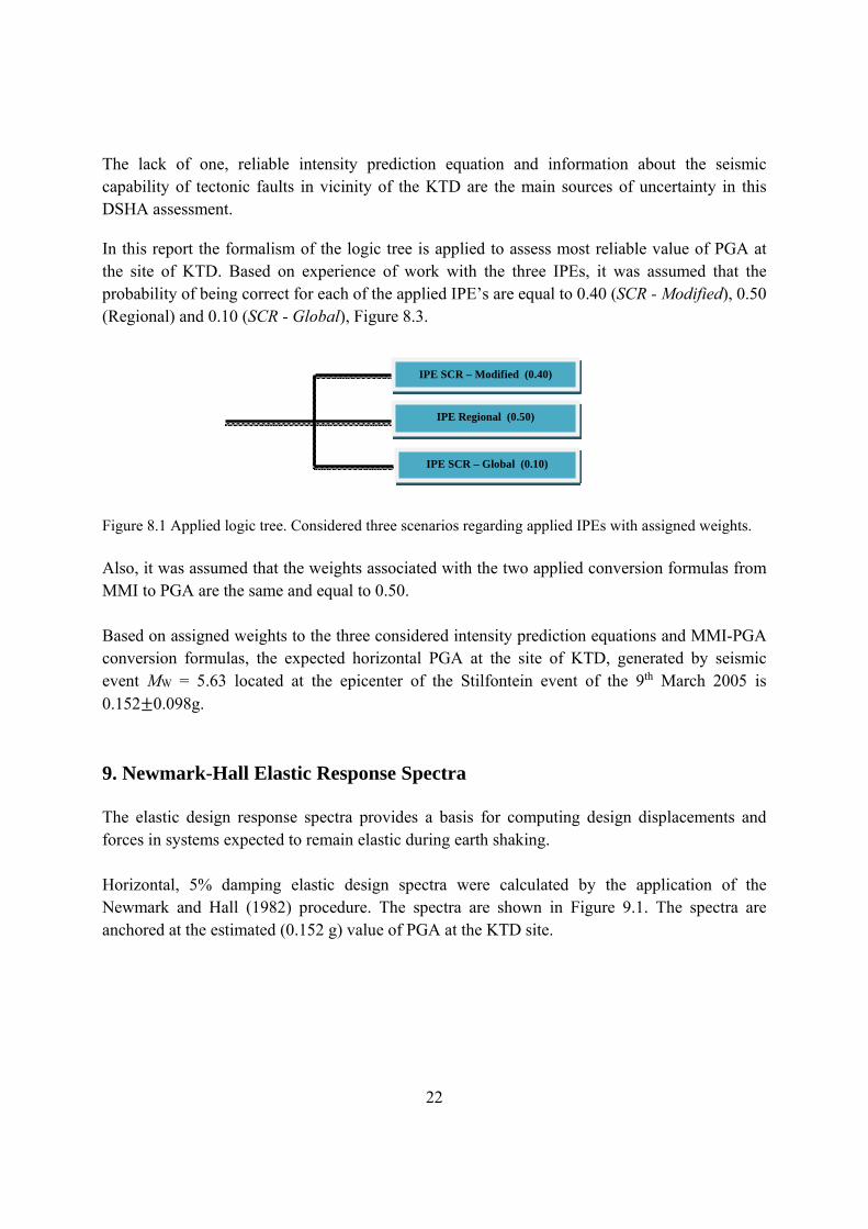
In this report the formalism of the logic tree is applied to assess most reliable value of PGA at the site of KTD. Based on experience of work with the three IPEs, it was assumed that the probability of being correct for each of the applied IPE’s are equal to 0.40 (SCR - Modified), 0.50 (Regional) and 0.10 (SCR - Global), Figure 8.3.

Figure 8.1 Applied logic tree. Considered three scenarios regarding applied IPEs with assigned weights.

Also, it was assumed that the weights associated with the two applied conversion formulas from MMI to PGA are the same and equal to 0.50. Based on assigned weights to the three considered intensity prediction equations and MMI-PGA conversion formulas, the expected horizontal PGA at the site of KTD, generated by seismic event MW = 5.63 located at the epicenter of the Stilfontein event of the 9th March 2005 is 0.152 0.098g.

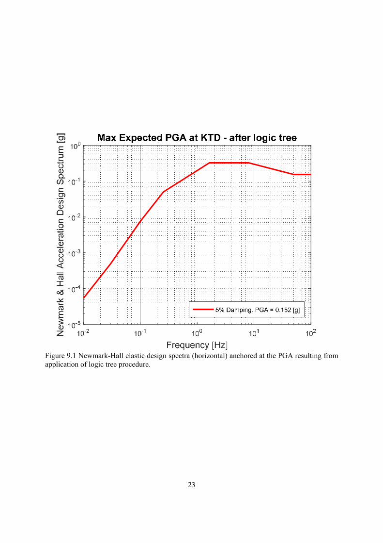
9. Newmark-Hall Elastic Response Spectra The elastic design response spectra provides a basis for computing design displacements and forces in systems expected to remain elastic during earth shaking. Horizontal, 5% damping elastic design spectra were calculated by the application of the Newmark and Hall (1982) procedure. The spectra are shown in Figure 9.1. The spectra are anchored at the estimated (0.152 g) value of PGA at the KTD site.

IPE SCR – Modified (0.40)

IPE Regional (0.50)

IPE SCR – Global (0.10)

23

Figure 9.1 Newmark-Hall elastic design spectra (horizontal) anchored at the PGA resulting from application of logic tree procedure.

24

10. Conclusions

A Deterministic Seismic Hazard Analysis (desk study) has been performed for site of the Kareerand Tailing Dam, Stilfontein. All known seismic events located within a 50 km radius of the site were used in the assessment.

The controlling event is determined as an event of magnitude MW = 5.63 0.11 located at the epicenter of 9th March 2005 Stilfontein event. The MW = 5.63 0.11 is considered as maximum possible, mine related seismic event magnitude, characteristic to the area. The predicted largest horizontal PGA at the site of dam is 0.152 0.098 g.

25

11. References Aki, K (1965). Maximum likelihood estimate of b in the formula log (N) = a − bM and its

confidence limits. Bulletin of the Earthquake Research Institute, Tokyo University 43, 237-239.

Bakun W. H. and Scotti O. [2006] “Regional intensity attenuation models for France and the estimation of magnitude and location of historical earthquakes”, Geophys. J. Int. 164, 596–610.

Brandt, M.B.C., M. Bejaichund, E.M. Kgaswane, and D.L. Roblin, 2005. Seismic History of Southern Africa. Seism. Series 37 of the Council for Geoscience. ISBN 1-919908-63-3.

Bernreuter, D.L. J.B. Savy, R.W. Mensing, and J.C. Chen (1989). Seismic Hazard Characterization of 69 Nuclear Plant Sites East of the Rocky Mountains. Report NUREG/CR-5250, Vols 1-8, prepared by Lawrence Livermore National Laboratory for the U.S. Nuclear Regulatory Commission.

Budnitz, R.J., G. Apostolakis, D.M. Boore, L.S. Cluff, K.J. Coppersmith, C.A. Cornell and P.A. Morris (1997). Recommendations for Probabilistic Seismic Hazard Analysis: Guidance on Uncertainty and Use of Experts. NUREG/CR-6372, UCR-ID-122160, Main Report 1. Prepared for Lawrence Livermore National Laboratory.

EERI Committee on Seismic Risk, (H.C. Shah, Chairman), (1984). Glossary of terms for probabilistic seismic risk and hazard analysis, Earthquake Spectra, 1, 33-36.

Geoclips (2013). Council for Geosciences, page 9. June 2013. Gibowicz, S. J., and Kijko, A., 1994. An Introduction to Mining Seismology. San Diego: Academic Press. Gutenberg B., Richter CF (1944). Frequency of earthquakes in California. (B). Bull. Seism. Soc.

Am, 34, 185–188. Hattingh, E, Bejaichund, M & Ramperthap, J (2006). Investigation of Ground Acceleration

Attenuation Relations for Key Areas in South Africa, Council for Geoscience, Pretoria. Report no. 2006–0050.

Kijko, A. (2004). Estimation of the Maximum Earthquake Magnitude, maxm . Pure and Applied

Geophysics, 161, 1–27. Kijko, A., and M.A. Sellevoll (1989). Estimation of earthquake hazard parameters from

incomplete data files, Part I, Utilization of extreme and complete catalogues with different threshold magnitudes, Bull. Seism. Soc. Am., 79, 645-654.

Kijko, A., and M.A. Sellevoll (1992). Estimation of earthquake hazard parameters from incomplete data files. Part II. Incorporation of magnitude heterogeneity. Bull. Seism. Soc. Am. 82, 120-134.

Kijko, A., A. Smit and M.A. Sellevoll, (2016). Estimation of earthquake hazard parameters from incomplete data files. Part III, Bull. Seism. Soc. Am., 106, 3, 1210-1222.

Kijko, A., and M. Singh (2011). Statistical tools for maximum possible earthquake magnitude estimation, Acta Geophysica. 59, 674-700.

Kramer, S. L. (1996). Geotechnical Earthquake Engineering. Englewood Cliffs, N.J. Prentice-Hill.

Lay, T. and T.C. Wallance (1995). Modern Global Seismology. London, Academic Press.

26

Mueller, C. (2010). The influence of the maximum magnitude on the seismic hazard estimates in the Central and Eastern United States, Bulletin of the Seismological Society of America, 100, 699-711.

Midzi, V. B. Zulu, B. Manzunzu, T. Mulabisana T., Pule, S. Myendeki and W. Gubela (2015). Macroseismic survey of the ML5.5, 2014 Orkney earthquake.

Newmark, N.M and W.J. Hall. (1982). Earthquake Spectra and Designs, EERI, Monograph Series, Berkley, 1982.

Page, R (1968). Aftershocks and microaftershocks. Bulletin of the Seismological Society of America 58, 1131-1168.

Quenouille, M.H. (1956), Note on bias in estimation, Biometrica, 43, 353-360. Reiter, L., (1990). Earthquake Hazard Analysis: Issues and Insights. New York: Columbia

University Press. Richter C (1958) Elementary Seismology. San Francisco, Freeman. Robson, D.S. and J.H. Whitlock (1964). Estimation of a truncation point, Biometrika, 51, 33-39. Shedlock, K.M. (1999). Seismic Hazard map of North and Central America and the

Caribbean. Annali Di Geophysica, 42, 977-997. Wald, D.J, Quitoriano, V, Heaton, TH & Kanamori, H (1999). Relationship between Peak

Ground Acceleration, Peak Ground Velocity, and Modified Mercalli Intensity in California. Earthquake Spectra 15(3), 557-564.

Wheeler, R.L. (2009). Methods of Mmax estimation east of the Rocky Mountains, U.S. Geological Survey Open-File Report 2009-1018, 44p.

Wells, D.L. and K.J. Coppersmith (1994). New empirical relationships among magnitude, rupture length, rupture width, rupture area, and surface displacement, Bull. Seism. Soc. Am., 84, 974-1002

27

APPENDICES

Appendix A

Seismicity of area surrounding the Kareerand Tailing Dam

in the radius of 50 km

YEAR MO DA LAT LONG MAGNITUDE

1966 5 18 -27.0000 27.0000 3.30 1966 7 25 -26.8000 26.5000 3.60 1966 8 30 -27.0000 26.7000 3.20 1966 9 4 -26.5000 27.1000 3.50 1966 9 12 -26.8000 26.7000 3.20 1966 11 10 -26.5000 27.1000 3.60 1967 1 20 -27.1000 26.8000 3.80 1967 2 19 -26.8000 26.5000 3.30 1967 2 22 -26.5000 27.0000 3.60 1967 3 3 -26.8000 26.5000 3.20 1967 3 9 -26.6000 26.9000 3.70 1967 4 6 -27.0000 26.6000 3.20 1967 4 24 -26.9000 26.6000 3.10 1967 6 1 -26.9000 26.7000 3.30 1967 8 8 -26.8000 26.8000 3.20 1967 8 24 -26.5000 27.1000 3.00 1967 9 14 -26.9000 26.7000 3.30 1967 9 23 -26.6000 26.8000 3.00 1967 11 1 -27.1000 27.2000 3.00 1967 12 5 -26.5000 27.1000 3.30 1967 12 15 -26.5000 27.1000 3.10 1967 12 18 -26.5000 27.1000 3.10 1967 12 23 -26.5000 27.1000 3.10 1968 1 5 -26.8000 26.7000 3.20 1968 1 9 -26.6000 27.0000 3.30 1968 1 10 -26.7000 26.9000 3.10 1968 1 13 -26.6000 27.1000 3.20 1968 1 24 -26.7000 26.6000 3.40 1968 1 24 -26.7000 26.6000 3.40 1968 2 1 -26.8000 26.7000 3.30 1968 2 8 -27.0000 26.6000 3.80 1968 2 10 -26.7000 27.1000 3.30 1968 2 22 -26.8000 26.5000 3.00 1968 3 7 -26.7000 26.7000 3.30 1968 4 7 -26.6000 27.1000 3.50 1968 5 3 -26.5600 27.2000 3.60 1968 5 9 -26.7000 27.0000 3.40 1968 5 21 -26.5000 27.1000 3.20 1968 5 29 -26.7000 26.5000 3.10 1968 6 13 -26.7000 26.5000 3.00 1968 6 24 -26.5000 27.1000 3.00 1968 7 5 -26.8000 26.8000 3.40 1968 8 16 -26.7100 26.7000 3.80 1968 9 16 -26.9000 26.6000 3.00 1968 9 20 -26.5000 27.0000 3.00 1968 10 9 -26.6000 26.8000 3.40 1968 10 20 -26.9000 26.5000 3.70 1968 12 7 -26.5000 27.0000 3.40 1968 12 25 -26.7500 26.8700 3.90 1969 1 18 -26.5000 27.1000 3.30 1969 1 22 -26.6500 26.9900 3.50 1969 1 24 -26.8100 26.7600 3.60 1969 1 28 -26.6000 27.1000 3.40 1969 2 1 -27.2000 27.1000 3.50 1969 2 21 -26.7600 26.8200 3.70 1969 2 27 -26.6000 27.1000 3.90 1969 4 12 -26.6000 27.1000 3.30 1969 4 20 -26.8000 27.2000 4.10 1969 5 2 -27.1400 26.5200 3.40 1969 5 15 -26.6400 26.8600 3.50 1969 6 2 -26.6700 26.8600 4.00 1969 6 13 -26.5000 27.1000 3.20 1969 6 22 -26.6000 27.1000 3.20 1969 7 12 -26.5000 26.9000 3.60 1969 7 23 -27.1000 27.0000 3.20 1969 8 1 -26.5500 27.1200 3.60

28

1969 8 12 -27.0000 27.1000 3.10 1969 8 13 -26.5000 27.1000 3.30 1969 8 19 -26.5000 27.1000 3.10 1969 8 21 -26.9000 26.6400 3.70 1969 8 30 -27.0000 27.0000 3.00 1969 8 30 -26.7700 26.8000 4.30 1969 9 10 -27.1000 26.9000 3.40 1969 9 17 -27.1000 27.0000 3.40 1969 9 20 -26.7000 27.0000 3.40 1969 10 25 -26.9000 26.9000 3.20 1969 10 30 -26.6800 26.9000 3.40 1969 11 20 -26.5000 27.1000 3.10 1969 11 21 -26.7300 26.9200 3.50 1969 11 21 -26.7000 26.9000 3.00 1969 11 26 -26.5000 27.1000 3.20 1969 12 1 -26.7000 26.7000 3.30 1969 12 30 -26.6000 27.0000 3.10 1970 1 6 -26.6800 26.7300 3.40 1970 1 20 -26.8000 26.9000 3.80 1970 1 22 -26.8100 26.8800 3.30 1970 3 4 -26.8200 26.6500 3.20 1970 3 12 -26.8000 26.6000 3.20 1970 3 21 -27.1000 26.5000 3.00 1970 3 24 -26.8300 26.9600 3.60 1970 4 3 -26.7000 26.9000 3.40 1970 5 21 -26.9000 26.7000 3.10 1970 5 23 -26.8200 26.9000 4.95 1970 5 27 -26.6000 27.1000 3.10 1970 6 2 -26.7000 27.0000 3.10 1970 6 22 -26.7000 26.9000 3.40 1970 6 24 -26.6800 26.9500 3.20 1970 7 1 -27.1000 27.1000 4.63 1970 7 7 -27.0000 26.8000 3.20 1970 7 8 -26.8800 26.5200 3.00 1970 7 16 -26.6000 26.9000 3.00 1970 7 24 -26.7000 27.2000 3.20 1970 7 30 -27.1000 26.7000 3.00 1970 8 5 -26.6800 26.9500 3.30 1970 8 6 -27.0000 26.6000 3.20 1970 8 16 -27.2000 27.1000 3.00 1970 8 25 -26.8200 26.6500 3.50 1970 9 3 -26.8100 26.8800 3.20 1970 9 11 -27.0400 27.2100 3.30 1970 9 12 -27.0000 26.8000 3.30 1970 9 25 -26.8400 26.8100 4.84 1970 9 25 -26.8300 26.8600 3.60 1970 9 29 -26.5900 27.0000 3.90 1970 10 17 -26.9000 26.9000 3.00 1970 10 26 -26.6000 27.1000 3.50 1970 10 31 -26.7800 26.8500 5.60 1970 11 9 -26.6000 27.2000 3.20 1970 11 13 -26.9000 27.2000 3.30 1970 11 19 -26.9000 26.9000 3.20 1970 11 19 -26.9000 26.9000 3.40 1970 11 27 -26.8200 26.6500 3.10 1970 12 6 -27.2000 27.0000 3.10 1970 12 25 -26.8000 26.5000 3.10 1971 1 10 -26.7700 26.7600 3.00 1971 1 12 -26.8000 26.6000 3.10 1971 1 14 -26.9000 27.0000 3.10 1971 1 19 -26.9300 26.5500 3.50 1971 1 23 -26.8000 26.4000 3.00 1971 1 23 -26.6800 26.7200 3.50 1971 1 25 -26.7600 26.7500 3.80 1971 2 1 -26.7600 26.7900 3.80 1971 2 5 -26.7600 26.7900 3.20 1971 2 21 -26.6900 26.9300 3.20 1971 2 22 -26.8500 26.6200 3.20 1971 2 24 -26.8200 26.6500 3.10 1971 2 27 -27.0100 26.6700 3.20 1971 3 6 -26.5500 27.0100 3.10 1971 3 16 -26.6300 26.8600 3.30 1971 4 10 -26.6900 26.9400 3.50 1971 4 14 -26.6800 26.9500 3.30 1971 5 4 -26.7100 26.8700 3.50 1971 5 5 -26.7900 27.1100 3.20 1971 6 6 -27.1000 27.1000 3.40 1971 6 6 -26.7700 26.7700 3.30 1971 6 23 -26.6700 26.5600 3.30 1971 7 21 -26.7600 26.8700 3.30 1971 9 1 -26.6600 26.7500 3.80 1971 9 6 -26.6400 26.8100 3.30 1971 9 9 -26.5600 26.6800 3.70 1971 9 10 -26.6400 26.8400 3.60 1971 9 14 -26.9200 26.6800 3.40 1971 10 18 -26.6900 26.8400 3.40 1971 11 12 -26.7200 26.7400 3.60 1972 2 7 -26.9300 26.7900 3.70 1972 3 17 -26.8100 26.7700 4.10 1972 5 9 -26.8900 26.6600 3.20 1972 5 10 -26.8100 26.7000 3.60 1972 5 17 -26.8000 26.7000 3.30 1972 5 17 -26.4500 26.8400 3.20 1972 6 20 -26.7800 26.6100 3.30 1972 7 9 -26.8100 26.8800 3.30

29

1972 8 5 -26.8500 26.7200 3.40 1972 8 16 -26.7400 26.6900 3.70 1972 8 24 -26.7400 27.0300 3.30 1972 8 25 -26.9000 26.7200 3.30 1972 9 7 -26.7900 26.8100 3.70 1972 10 14 -26.5000 26.9300 3.30 1972 11 1 -26.9000 26.8700 4.40 1972 11 12 -26.9000 26.9200 3.20 1972 11 14 -26.8900 26.7800 3.40 1972 12 8 -26.8800 26.5200 3.10 1972 12 10 -26.6500 26.6700 3.70 1972 12 18 -26.6100 26.8600 4.00 1972 12 27 -26.8700 26.7900 3.80 1973 1 31 -26.7900 26.7100 3.30 1973 3 8 -26.8500 26.7100 3.30 1973 4 15 -26.8600 26.7600 3.30 1973 4 16 -26.7700 26.7700 3.90 1973 5 23 -26.7600 26.4800 3.30 1973 5 31 -26.8400 26.8100 3.30 1973 6 9 -26.8800 26.6400 3.10 1973 6 21 -26.9600 27.0200 3.20 1973 6 22 -26.6900 26.6100 3.30 1973 8 7 -26.7800 26.7700 4.10 1973 8 14 -26.7600 26.7000 3.80 1973 8 31 -26.8100 26.9000 3.30 1973 9 30 -26.8100 26.6600 3.50 1973 10 5 -26.8200 26.9500 3.50 1973 11 7 -26.9400 26.9500 4.30 1973 11 13 -26.7900 26.7800 4.20 1973 11 13 -26.7800 26.7300 3.80 1973 12 15 -26.5800 26.9900 3.50 1973 12 19 -26.7500 26.9900 4.95 1973 12 30 -26.8600 26.8000 3.40 1974 1 5 -26.5300 26.9400 3.20 1974 1 7 -26.7800 26.9400 3.50 1974 3 17 -26.8300 26.7500 4.20 1974 4 3 -26.7200 26.6900 3.30 1974 4 17 -26.8100 26.8200 3.40 1974 6 14 -26.8000 26.5200 4.10 1974 6 23 -26.8800 26.7300 3.50 1974 7 7 -26.8600 26.8500 3.40 1974 7 23 -26.8200 26.9200 4.80 1974 8 13 -26.8100 26.7800 3.40 1974 12 9 -26.8100 26.7700 3.40 1974 12 9 -26.7800 26.7500 3.40 1974 12 15 -26.8700 26.5400 3.80 1975 2 8 -26.9200 26.7200 3.80 1975 2 26 -26.7000 26.5900 3.50 1975 5 31 -26.7900 26.8300 3.50 1975 6 4 -26.7200 26.7600 3.90 1975 7 15 -27.0000 26.9600 3.40 1975 7 15 -26.8300 26.8200 3.70 1975 8 19 -26.8300 26.7600 3.60 1975 10 27 -26.9000 26.7700 3.60 1975 12 29 -26.9300 26.8100 3.40 1976 1 19 -26.7000 26.5000 3.20 1976 1 24 -26.7600 26.7200 3.50 1976 1 26 -26.8300 26.9000 3.60 1976 1 29 -26.4600 27.0400 3.50 1976 2 8 -26.5300 27.0900 3.50 1976 3 6 -27.0700 27.3200 3.30 1976 3 13 -26.8900 26.7600 3.50 1976 4 1 -27.2500 26.9200 3.30 1976 6 21 -26.8900 27.3100 3.50 1976 6 30 -26.8900 26.8600 3.50 1976 7 31 -26.8100 26.7000 3.80 1976 7 31 -26.7700 26.4500 3.80 1976 8 3 -26.9200 26.7700 3.70 1976 8 4 -26.8300 26.8200 3.40 1976 9 4 -26.7800 26.8200 3.50 1976 9 24 -26.8700 26.9100 3.80 1976 9 24 -26.7700 26.8400 3.50 1976 12 10 -26.9400 27.3400 3.50 1976 12 18 -26.7800 26.5900 3.50 1977 1 8 -26.7700 26.7400 4.20 1977 1 20 -26.8000 26.8000 3.10 1977 2 17 -26.8700 26.8200 3.30 1977 3 6 -26.6600 26.5500 4.20 1977 4 7 -26.9000 26.6500 3.80 1977 4 7 -26.8900 26.7400 5.00 1977 4 19 -26.9100 26.9700 3.50 1977 4 26 -26.8600 26.7500 3.70 1977 6 21 -26.9900 27.1000 3.40 1977 7 11 -26.8600 26.7500 4.00 1977 8 8 -26.9700 26.8000 3.00 1977 9 2 -26.7800 26.7200 3.80 1977 9 20 -26.8400 26.7900 3.00 1977 9 26 -26.7700 26.6200 3.60 1977 9 27 -27.0200 26.7500 3.30 1977 10 6 -26.8800 26.6900 4.20 1977 10 13 -26.8700 26.7600 3.00 1977 10 31 -26.8700 26.7800 3.10 1977 11 19 -26.5000 26.9700 3.50 1977 12 1 -26.9200 26.6900 3.30 1977 12 6 -26.9100 26.6300 4.10

30

1977 12 20 -26.8800 26.4800 3.10 1978 1 19 -26.8600 26.7200 4.30 1978 2 4 -26.8900 26.7300 3.40 1978 2 8 -26.9300 26.8400 3.20 1978 2 18 -26.4900 27.0100 3.60 1978 2 19 -27.0800 26.8700 3.00 1978 2 24 -26.8000 26.7000 3.30 1978 3 18 -26.8100 26.7100 3.70 1978 3 31 -27.0600 26.8000 3.30 1978 4 7 -26.9800 26.6700 3.00 1978 4 26 -26.8100 26.7400 3.90 1978 5 8 -26.9600 26.9000 3.00 1978 5 10 -26.7000 26.7000 3.20 1978 5 27 -26.8800 26.8200 4.00 1978 6 7 -26.9600 26.8600 3.40 1978 6 15 -26.8100 26.6700 3.50 1978 6 24 -27.0300 27.2200 3.40 1978 7 21 -26.8700 26.6800 3.50 1978 8 22 -26.8600 26.6200 3.50 1978 8 29 -26.8000 26.6400 3.70 1978 9 17 -26.8900 26.7200 3.30 1978 10 11 -27.0200 26.9600 3.50 1978 10 12 -26.9000 26.9000 3.50 1978 10 21 -26.7800 26.6800 3.60 1978 11 2 -26.7600 26.6900 3.90 1978 12 9 -26.7800 26.7900 3.90 1979 1 24 -26.8500 26.6500 4.95 1979 1 25 -26.8600 26.7200 4.00 1979 1 25 -26.8100 26.6500 5.28 1979 3 2 -26.8100 26.6600 3.60 1979 3 31 -26.8300 26.7100 3.50 1979 4 5 -26.8300 26.6500 3.10 1979 4 6 -26.8500 26.7300 5.17 1979 4 7 -26.9500 26.7500 3.30 1979 4 13 -26.8800 26.7500 3.20 1979 5 23 -26.7900 26.7700 3.90 1979 6 18 -26.8300 26.6700 3.60 1979 7 8 -26.7300 26.6300 3.30 1979 7 11 -26.9300 26.7000 3.10 1979 8 18 -26.8200 26.8200 3.70 1979 9 23 -26.9700 26.6800 3.10 1979 10 2 -26.8400 26.6600 4.00 1979 10 4 -26.8400 26.7800 3.60 1979 10 12 -26.9000 26.7500 3.30 1979 11 7 -26.7300 26.6600 3.50 1979 11 16 -26.8700 26.7200 3.70 1979 12 13 -26.9000 26.9100 3.50 1980 1 18 -26.8300 26.7200 3.30 1980 2 4 -26.4900 27.0400 3.20 1980 2 6 -26.8200 26.6500 3.70 1980 2 27 -27.0200 26.8900 3.20 1980 2 28 -26.9400 26.6900 3.20 1980 3 4 -26.8900 26.7600 3.80 1980 3 6 -26.8600 26.4100 3.70 1980 4 11 -26.7600 26.5700 3.00 1980 4 26 -26.8700 26.6500 3.20 1980 4 30 -26.9000 26.7200 3.60 1980 5 6 -26.9300 27.0000 4.84 1980 5 13 -26.8800 26.6100 3.20 1980 5 13 -26.8700 26.8400 3.20 1980 5 19 -26.8400 26.6900 3.30 1980 6 12 -26.9800 26.9700 5.06 1980 6 13 -26.8600 26.8100 3.30 1980 6 13 -26.8500 26.7700 5.06 1980 7 9 -26.8600 26.7600 3.40 1980 7 10 -26.8800 26.7500 3.90 1980 7 18 -26.7800 26.7000 3.60 1980 7 26 -26.8700 26.8500 3.50 1980 8 2 -26.9900 26.8100 3.00 1980 8 28 -26.9000 26.7000 3.90 1980 9 14 -26.7600 26.6800 3.60 1980 9 14 -26.7500 26.6600 3.40 1980 9 25 -26.8500 26.6800 3.00 1980 10 23 -26.8300 26.7200 3.30 1980 11 4 -26.8400 26.6800 3.00 1980 11 6 -26.7000 26.7000 3.60 1980 11 7 -26.7700 26.7200 3.40 1980 11 8 -26.8400 26.7100 3.30 1980 11 14 -26.8400 26.7900 3.20 1980 11 14 -26.7600 26.7900 3.30 1980 11 20 -26.8000 26.7300 3.80 1980 12 11 -26.8100 26.8000 3.50 1981 1 24 -26.8900 26.8100 3.00 1981 1 30 -26.8500 26.7100 3.00 1981 2 2 -26.9100 26.7100 3.10 1981 2 5 -26.9100 26.7400 3.00 1981 2 8 -26.8100 26.8200 3.60 1981 2 18 -26.7900 26.6500 4.95 1981 3 3 -26.9200 26.7500 3.20 1981 3 14 -26.8600 26.7500 3.40 1981 3 16 -26.6200 26.9300 3.50 1981 4 4 -26.8700 26.7400 3.10 1981 4 15 -26.7700 26.6600 3.30 1981 4 22 -26.7400 27.0200 3.10 1981 5 7 -26.7600 26.5900 3.30

31

1981 5 9 -26.8000 26.5900 3.50 1981 5 12 -26.7900 26.6900 3.10 1981 5 21 -26.8900 26.7600 3.10 1981 5 27 -26.8700 26.8800 3.20 1981 5 30 -26.7300 26.6300 3.00 1981 6 4 -26.8500 26.8600 3.10 1981 6 5 -26.8500 26.7400 3.00 1981 6 18 -26.5400 27.1300 3.40 1981 7 5 -26.8800 26.6600 3.10 1981 7 13 -26.8000 26.6700 3.20 1981 8 7 -26.9400 26.8800 3.10 1981 8 9 -26.8000 26.7500 3.30 1981 8 14 -26.8000 26.8000 3.90 1981 9 5 -26.8300 26.6900 3.40 1981 9 19 -26.7600 26.6900 3.30 1981 10 8 -26.9500 26.8400 5.70 1981 10 22 -26.8800 26.7700 3.10 1981 11 28 -26.9800 26.7500 3.20 1981 11 30 -26.8600 26.7300 3.30 1981 12 4 -26.5600 27.0800 3.10 1981 12 6 -26.4900 27.1200 3.30 1981 12 24 -26.8500 26.6900 3.30 1981 12 24 -26.8100 26.7700 3.30 1981 12 25 -26.7800 26.5800 3.20 1981 12 28 -26.8300 26.6800 3.10 1982 1 5 -26.8500 26.6700 3.10 1982 1 6 -26.8500 26.6400 3.00 1982 1 11 -26.7600 26.5200 3.50 1982 1 18 -26.9100 26.7800 3.00 1982 1 29 -26.7700 26.6300 3.30 1982 1 29 -26.7500 26.6600 3.20 1982 2 10 -26.8300 26.7200 3.10 1982 2 10 -26.8000 26.6900 3.40 1982 2 16 -26.7800 26.6200 3.50 1982 3 2 -26.5900 26.7000 3.20 1982 3 31 -26.8600 26.7500 3.10 1982 4 2 -26.8800 26.7500 3.20 1982 4 9 -26.7500 26.5900 4.52 1982 4 26 -26.7900 26.6900 3.40 1982 4 27 -26.8500 26.6400 3.80 1982 5 10 -26.8500 26.6200 3.00 1982 5 28 -26.8900 26.6900 3.60 1982 5 28 -26.8600 26.6600 3.20 1982 6 18 -26.8900 26.7900 3.70 1982 6 20 -26.8700 26.6700 3.10 1982 6 23 -26.8300 26.7200 3.20 1982 6 27 -26.7600 26.5400 3.60 1982 6 28 -26.8800 26.8100 3.40 1982 9 17 -26.9000 26.7300 3.10 1982 9 17 -26.8300 26.6700 3.30 1982 9 29 -26.8500 26.7000 3.00 1982 10 1 -26.8500 26.7100 3.60 1982 11 1 -26.8800 26.7100 3.50 1982 11 12 -26.9100 26.7200 5.17 1982 11 29 -26.9500 26.7500 3.30 1982 12 6 -26.8800 26.7300 3.20 1982 12 11 -26.8700 26.6700 4.74 1982 12 11 -26.8600 26.6800 3.10 1982 12 11 -26.7300 26.7000 4.09 1982 12 11 -26.7100 26.5500 3.10 1982 12 16 -26.8900 26.7300 3.00 1982 12 21 -26.8800 26.7100 3.80 1982 12 21 -26.8500 26.7200 3.20 1982 12 28 -26.6900 26.5400 3.40 1983 1 3 -26.8200 26.6600 4.74 1983 1 5 -26.8100 26.6600 3.20 1983 1 14 -26.8800 26.8600 3.20 1983 2 8 -26.8200 26.6100 3.70 1983 2 18 -26.9900 26.8000 3.30 1983 3 19 -26.9100 26.7600 3.40 1983 4 4 -26.8800 26.6500 3.40 1983 4 8 -26.9500 26.7100 3.00 1983 4 8 -26.8900 26.6800 3.00 1983 4 13 -26.8700 26.6400 3.70 1983 4 14 -26.8800 26.6200 4.63 1983 4 14 -26.8700 26.7500 3.20 1983 4 17 -26.8600 26.7100 3.00 1983 4 24 -26.9200 26.7500 3.20 1983 4 25 -26.8500 26.7000 3.10 1983 4 27 -26.8800 26.7300 3.50 1983 5 5 -26.8900 26.7300 3.10 1983 5 17 -26.8300 26.6600 5.06 1983 5 18 -26.8600 26.7700 3.50 1983 5 19 -26.8700 26.7300 3.00 1983 5 28 -26.8500 26.7500 3.10 1983 6 5 -26.8900 26.7300 3.10 1983 6 6 -26.8800 26.7500 5.39 1983 6 6 -26.8700 26.7400 4.30 1983 6 11 -26.9200 26.7200 3.30 1983 6 17 -26.9500 26.7900 3.40 1983 6 20 -26.9500 26.6700 3.30 1983 6 21 -26.9600 26.8500 3.10 1983 6 27 -27.0000 26.7200 3.20 1983 6 29 -26.8000 26.6900 3.30 1983 6 30 -26.8800 26.8100 3.00

32

1983 7 7 -26.9100 26.7000 3.20 1983 7 7 -26.8500 26.6100 3.40 1983 7 9 -26.9600 26.7900 3.00 1983 8 3 -26.8900 26.7000 3.00 1983 8 6 -26.8300 26.6200 3.40 1983 8 15 -26.9500 26.7300 3.40 1983 9 7 -26.9500 26.7200 3.10 1983 9 11 -26.8200 26.7500 4.00 1983 9 18 -26.9100 26.7100 3.30 1983 9 26 -26.7500 26.6800 3.00 1983 12 7 -26.8800 26.6200 4.84 1984 1 28 -26.9000 26.6300 5.08 1984 1 28 -26.8200 26.7000 5.28 1984 2 3 -26.9700 26.8500 3.40 1984 2 9 -27.0000 26.8000 3.10 1984 2 14 -26.8300 26.7500 3.00 1984 2 22 -26.7100 26.6300 3.30 1984 2 23 -26.8300 26.7100 3.30 1984 2 24 -26.8000 26.6100 3.40 1984 3 5 -26.8000 26.6300 3.90 1984 3 15 -26.9600 26.7900 3.00 1984 3 27 -26.8700 26.6800 3.00 1984 3 30 -26.9400 26.8700 3.00 1984 4 17 -26.8700 26.6900 3.10 1984 4 24 -26.9200 26.9400 3.20 1984 5 1 -26.8800 26.8400 3.10 1984 5 2 -26.9000 26.7700 3.30 1984 5 4 -26.8300 26.6300 4.84 1984 5 16 -26.9200 26.6900 3.00 1984 5 18 -26.9500 26.7600 3.00 1984 6 9 -26.9400 26.7800 3.00 1984 6 20 -26.9100 26.7600 3.10 1984 6 20 -26.8800 26.7600 3.10 1984 6 25 -26.9400 26.7800 3.40 1984 7 4 -26.9200 26.7100 3.40 1984 7 5 -26.8100 26.7500 4.00 1984 7 13 -26.8800 26.7500 3.20 1984 7 24 -26.8400 26.5700 3.10 1984 7 28 -26.8500 26.5300 3.00 1984 7 29 -26.8400 26.4500 3.00 1984 7 31 -26.9300 26.7400 3.00 1984 8 5 -26.8600 26.8100 3.10 1984 8 9 -26.8200 26.7000 3.00 1984 8 11 -26.8300 26.6400 5.06 1984 8 11 -26.8000 26.6800 3.60 1984 8 11 -26.8000 26.7200 3.90 1984 8 15 -26.8700 26.6400 3.50 1984 9 14 -26.9600 26.7000 3.10 1984 9 15 -26.7800 26.6600 3.80 1984 9 18 -26.9800 26.7200 3.00 1984 9 22 -26.8300 26.6100 3.20 1984 10 4 -26.8000 26.6800 3.50 1984 10 15 -26.7000 26.7400 3.40 1984 10 18 -26.8100 26.6100 3.70 1984 10 30 -26.9400 26.8100 3.30 1984 11 19 -26.9600 26.7200 3.10 1984 11 22 -26.9500 26.8100 3.00 1984 11 24 -26.8100 26.7000 3.20 1984 11 30 -26.8800 26.6900 3.30 1984 12 4 -26.8500 26.7900 3.60 1984 12 15 -26.8900 26.7100 3.70 1984 12 18 -26.8500 26.7600 3.50 1984 12 26 -26.8900 26.7500 3.30 1984 12 28 -26.9300 26.7600 3.00 1985 1 4 -26.7500 26.5700 3.20 1985 1 14 -26.8500 26.6700 3.60 1985 1 16 -26.8100 26.6300 3.50 1985 1 17 -26.9300 26.7300 3.20 1985 1 18 -26.9400 26.8200 3.20 1985 1 19 -26.7700 26.5600 3.10 1985 2 6 -26.8300 26.8300 3.30 1985 3 2 -26.7700 26.7000 3.40 1985 3 6 -26.8500 26.7100 3.60 1985 3 8 -26.8500 26.6400 3.40 1985 3 20 -26.8800 26.7400 3.70 1985 3 22 -26.8900 26.7300 3.40 1985 3 25 -26.8900 26.7400 3.50 1985 3 29 -26.8300 26.7500 3.00 1985 4 2 -26.8600 26.6800 3.20 1985 4 6 -26.7800 26.7600 3.70 1985 4 9 -26.9200 26.7700 3.00 1985 4 14 -26.8100 26.6400 3.20 1985 4 14 -26.8000 26.6800 3.40 1985 4 18 -26.8700 26.8100 3.00 1985 4 21 -26.7200 26.7300 3.20 1985 4 24 -26.8000 26.6100 4.95 1985 5 10 -26.9500 26.8000 3.10 1985 5 16 -26.9700 26.8000 3.00 1985 5 26 -26.7900 26.6500 4.95 1985 6 7 -26.8200 26.6600 3.10 1985 6 8 -26.7400 26.6700 4.30 1985 6 22 -26.7900 26.7400 3.40 1985 7 3 -26.9100 26.7300 3.30 1985 7 4 -26.7700 26.6000 4.20 1985 7 6 -26.7700 26.6000 3.20

33

1985 7 8 -26.8800 26.7400 3.00 1985 7 16 -26.9300 26.7400 3.10 1985 7 30 -26.8500 26.6800 4.63 1985 7 30 -26.8300 26.7800 3.10 1985 8 3 -26.9100 26.7600 3.00 1985 8 8 -26.9000 26.6900 3.20 1985 8 9 -26.9200 26.7500 3.10 1985 8 11 -26.7800 26.7500 3.80 1985 8 13 -26.8800 26.7700 3.10 1985 8 27 -26.8100 26.7100 3.00 1985 8 28 -26.8900 26.6700 3.00 1985 9 5 -26.9400 26.8200 3.10 1985 9 20 -26.8600 26.6800 3.30 1985 9 21 -26.8200 26.6700 3.20 1985 9 24 -26.9300 26.7800 3.10 1985 10 2 -26.9800 26.7200 3.20 1985 10 2 -26.8100 26.6300 3.50 1985 10 6 -26.9000 26.7100 3.10 1985 10 8 -26.9200 26.6100 3.40 1985 10 9 -26.8900 26.6400 3.30 1985 10 11 -26.9100 26.7000 3.10 1985 10 27 -26.8000 26.6000 3.30 1985 11 1 -26.9100 26.7000 3.30 1985 11 2 -26.7600 26.7800 3.50 1985 11 9 -26.8800 26.7800 3.30 1985 11 21 -26.9200 26.7000 3.10 1985 12 19 -26.9100 26.7100 3.10 1985 12 20 -26.8700 26.8000 3.00 1985 12 27 -26.8500 26.8500 3.00 1986 1 1 -26.8000 26.6700 5.17 1986 1 9 -26.9000 26.8300 3.30 1986 1 9 -26.8700 26.7500 4.52 1986 1 22 -26.8300 26.8700 4.74 1986 1 27 -26.8100 26.7100 4.63 1986 1 27 -26.8000 26.8200 3.70 1986 1 29 -26.8900 26.6900 3.10 1986 2 23 -26.8000 26.6500 4.00 1986 2 24 -26.7700 26.5900 3.40 1986 3 19 -26.9100 26.8200 3.20 1986 3 21 -26.8700 26.8100 3.20 1986 4 9 -26.8800 26.5700 3.00 1986 4 9 -26.8700 26.5900 3.20 1986 4 19 -26.9400 26.7300 3.50 1986 4 21 -26.8900 26.7100 3.10 1986 4 22 -26.9800 26.6300 3.20 1986 5 14 -26.8900 26.7400 3.20 1986 5 29 -26.9500 26.7900 3.00 1986 6 4 -26.7700 26.7300 3.10 1986 6 8 -26.9700 26.8100 3.10 1986 6 29 -26.8400 26.6900 3.20 1986 7 8 -26.8800 26.7300 3.30 1986 7 19 -26.9300 26.7100 3.00 1986 7 21 -26.8900 26.7100 3.10 1986 7 22 -26.9200 26.6900 4.52 1986 7 31 -26.9500 26.7600 3.00 1986 8 8 -26.9000 26.7500 3.30 1986 8 9 -26.9600 26.7900 3.00 1986 8 11 -26.9100 26.6000 5.17 1986 8 21 -26.8900 26.7000 3.30 1986 8 26 -26.8800 26.7500 3.00 1986 8 29 -26.9500 26.7000 3.30 1986 9 24 -26.7800 26.6900 3.40 1986 10 2 -26.8400 26.7300 3.20 1986 10 5 -26.8900 26.7200 3.00 1986 10 10 -26.9500 26.7800 3.00 1986 10 28 -27.0000 26.7500 3.10 1986 10 28 -26.9400 26.7500 5.70 1986 11 6 -27.0000 26.8000 3.10 1986 11 7 -26.9200 26.7200 3.30 1986 11 13 -26.9000 26.7500 5.28 1986 11 19 -26.8600 26.6600 4.10 1986 11 24 -27.0300 26.7900 3.20 1986 12 8 -26.8500 26.6300 3.10 1986 12 9 -26.9100 26.6900 3.00 1987 2 6 -26.8800 26.7500 3.30 1987 3 4 -26.9100 26.7900 3.00 1987 3 7 -26.9900 26.7400 3.00 1987 3 17 -26.8900 26.7100 3.20 1987 3 20 -26.7800 26.6200 3.00 1987 4 2 -26.9000 26.6300 3.10 1987 4 9 -26.9700 26.7700 3.10 1987 4 9 -26.9400 26.7500 3.30 1987 4 12 -26.8300 26.6800 3.20 1987 4 14 -26.8500 26.7000 5.17 1987 5 6 -26.9400 26.8300 3.00 1987 5 20 -26.8800 26.6900 3.10 1987 5 20 -26.8600 26.7200 3.70 1987 5 26 -26.9300 26.7700 3.60 1987 5 29 -26.8400 26.6600 5.06 1987 7 4 -26.9100 26.7200 3.40 1987 7 6 -26.8700 26.6200 3.30 1987 7 24 -26.8500 26.6800 3.30 1987 7 25 -26.8100 26.7700 3.00 1987 7 30 -26.9000 26.8700 3.10 1987 7 30 -26.7800 26.6900 5.17

34

1987 8 4 -26.8500 26.7100 3.50 1987 8 25 -26.8500 26.7800 3.10 1987 9 7 -26.9300 26.7200 3.60 1987 9 12 -26.9300 26.7400 3.00 1987 9 12 -26.8400 26.6300 3.60 1987 9 30 -26.7800 26.7000 5.06 1987 10 12 -26.9300 26.6600 3.10 1987 11 22 -26.7800 26.7300 3.10 1987 12 19 -26.7600 26.4900 3.60 1987 12 23 -26.9700 26.8100 3.00 1987 12 28 -26.8300 26.6600 3.30 1988 1 5 -26.9100 26.7000 5.28 1988 1 6 -26.8200 26.5500 3.20 1988 1 30 -26.8400 26.5900 3.40 1988 1 31 -26.8900 26.6400 3.00 1988 2 26 -26.8500 26.6400 4.09 1988 3 4 -26.9700 26.8100 3.10 1988 3 12 -26.9600 26.5700 3.10 1988 3 12 -26.8000 26.6300 3.50 1988 3 16 -26.8000 26.6100 3.20 1988 3 24 -26.8700 26.6200 3.20 1988 4 11 -26.8200 26.7700 3.00 1988 4 28 -26.8500 26.7400 3.00 1988 5 15 -26.8200 26.5800 3.50 1988 6 4 -26.8900 26.7000 3.30 1988 6 4 -26.8200 26.7200 3.20 1988 6 16 -26.7800 26.7400 4.00 1988 7 5 -26.8500 26.7000 3.20 1988 7 22 -26.7900 26.6300 3.10 1988 7 31 -26.8300 26.8000 3.10 1988 8 9 -26.9500 26.7900 3.10 1988 8 11 -26.8400 26.6400 3.70 1988 8 17 -26.8400 26.5900 3.60 1988 8 31 -26.8100 26.7100 3.40 1988 9 11 -26.8600 26.7300 3.40 1988 9 12 -26.8900 26.6500 4.84 1988 9 15 -26.8500 26.6800 3.50 1988 9 18 -26.8400 26.8200 3.10 1988 10 8 -26.8300 26.6300 3.00 1988 10 13 -26.8200 26.7000 3.10 1988 10 14 -26.8400 26.7300 3.10 1988 10 28 -26.9100 26.7900 3.10 1988 10 28 -26.8700 26.8400 3.10 1988 11 3 -26.8300 26.7400 3.20 1988 11 14 -26.8700 26.6700 3.10 1988 11 28 -26.9700 26.6400 3.10 1988 12 8 -26.8700 26.6300 3.10 1988 12 15 -26.8300 26.7900 4.95 1988 12 22 -26.9500 26.6500 4.74 1988 12 23 -26.8300 26.6500 3.20 1989 1 4 -26.9000 26.7700 3.20 1989 1 20 -26.8100 26.7200 3.30 1989 2 9 -26.9200 26.7300 3.00 1989 2 20 -26.8300 26.6900 3.60 1989 3 10 -26.9600 26.8100 3.00 1989 3 14 -26.8800 26.7100 3.20 1989 3 15 -26.8900 26.7600 3.00 1989 3 16 -26.8200 26.7300 3.10 1989 3 30 -26.8100 26.7700 4.84 1989 4 2 -26.7900 26.6100 3.70 1989 4 2 -26.7700 26.6700 3.50 1989 4 27 -26.9100 26.6900 3.60 1989 5 3 -26.7800 26.6200 5.06 1989 7 23 -26.8600 26.7600 4.84 1989 10 7 -26.8900 26.6300 4.84 1989 10 8 -26.9100 26.6500 5.17 1989 10 23 -26.8700 26.7300 3.80 1989 11 4 -26.9000 26.7300 3.50 1989 11 20 -26.9300 26.6400 3.70 1989 11 27 -26.8800 26.5300 3.90 1989 12 2 -26.9000 26.6900 3.60 1990 1 14 -26.9400 26.8300 3.60 1990 1 21 -26.8300 26.7600 3.50 1990 2 7 -26.8300 26.6800 4.74 1990 2 8 -26.8400 26.7500 4.74 1990 2 27 -26.9500 26.6700 4.63 1990 3 3 -26.9500 26.7200 5.28 1990 3 15 -26.8700 26.6400 3.50 1990 3 15 -26.8000 26.7000 4.30 1990 4 26 -26.9300 26.7200 3.20 1990 4 27 -26.7600 26.5500 3.10 1990 5 1 -26.8900 26.7500 3.00 1990 5 6 -26.6600 26.6100 3.40 1990 5 19 -26.9000 26.5900 3.30 1990 5 20 -26.8500 26.7300 3.00 1990 5 20 -26.8100 26.7300 4.52 1990 5 24 -26.8700 26.6300 3.00 1990 5 27 -26.9200 26.8100 3.30 1990 6 11 -26.8700 26.7100 3.00 1990 6 12 -26.8300 26.6400 3.30 1990 7 18 -26.8600 26.6200 4.84 1990 7 27 -26.8000 26.7400 4.30 1990 8 9 -26.9100 26.7500 3.00 1990 9 16 -26.9100 26.7700 3.30 1990 9 22 -26.8700 26.8100 3.10

35

1990 10 18 -26.9700 26.6000 3.50 1990 10 22 -26.9700 26.6700 3.80 1990 11 15 -26.8300 26.7000 3.70 1990 11 26 -26.7900 26.5600 3.60 1990 12 7 -26.8300 26.5900 3.40 1990 12 24 -26.7800 26.7000 3.80 1990 12 25 -26.8700 26.6000 3.20 1990 12 28 -26.8200 26.8400 3.20 1991 1 3 -26.9000 26.8100 3.00 1991 1 8 -26.8600 26.7000 3.10 1991 2 2 -26.7900 26.4600 3.40 1991 2 3 -26.9200 26.6600 3.10 1991 2 6 -26.8200 26.6300 3.90 1991 2 7 -26.8200 26.8300 3.30 1991 2 15 -26.8800 26.6200 3.20 1991 2 27 -26.8800 26.6700 3.20 1991 2 27 -26.8500 26.8900 3.10 1991 3 1 -26.8300 26.7000 3.20 1991 3 15 -26.8600 26.6400 3.00 1991 3 19 -26.9100 26.6400 3.00 1991 3 21 -26.9700 26.7500 3.40 1991 3 22 -26.8500 26.5900 3.20 1991 4 11 -26.8700 26.7200 3.20 1991 5 2 -26.8300 26.6500 3.30 1991 5 30 -26.8300 26.7000 3.40 1991 5 31 -26.8400 26.6200 3.10 1991 6 5 -26.9200 26.7800 3.00 1991 6 7 -26.8100 26.6200 3.40 1991 6 8 -26.8600 26.7500 3.60 1991 6 10 -26.8700 26.7100 4.95 1991 6 14 -26.8200 26.5900 3.50 1991 6 15 -26.9600 26.8200 3.00 1991 6 24 -26.8500 26.8500 3.40 1991 6 29 -26.7800 26.6600 3.50 1991 7 12 -26.8400 26.5700 4.00 1991 7 17 -26.7100 26.7200 3.80 1991 7 23 -26.7400 26.6800 3.60 1991 7 30 -26.9000 26.8200 3.00 1991 8 1 -26.9000 26.6600 3.10 1991 8 14 -26.9100 26.8300 3.30 1991 8 25 -26.8700 26.7500 3.20 1991 8 31 -26.9400 26.5800 3.30 1991 8 31 -26.7900 26.5500 3.40 1991 9 4 -26.9800 26.8000 3.30 1991 9 10 -26.8200 26.5600 3.50 1991 9 14 -26.9400 26.6900 3.00 1991 9 16 -26.8400 26.7300 3.50 1991 9 30 -26.8600 26.6500 3.50 1991 10 3 -26.8900 26.6400 3.30 1991 10 27 -26.8500 26.7500 3.90 1991 11 3 -26.9400 26.7400 5.28 1991 11 6 -26.8000 26.7200 3.30 1991 11 10 -26.6300 26.5400 3.00 1991 11 22 -26.7900 26.6300 3.50 1991 11 24 -26.8100 26.7000 3.00 1991 12 1 -26.9000 26.7700 5.06 1991 12 1 -26.8500 26.6200 3.10 1991 12 11 -26.8800 26.6300 3.10 1991 12 13 -26.9000 26.6100 3.30 1991 12 15 -26.8700 26.7400 3.60 1991 12 23 -26.9200 26.7700 3.30 1991 12 24 -26.9100 26.7300 3.80 1991 12 24 -26.8700 26.7500 3.20 1992 1 8 -26.8300 26.6800 3.40 1992 1 18 -26.8900 26.7300 4.63 1992 1 18 -26.8800 26.7200 3.30 1992 2 1 -26.8000 26.6500 3.30 1992 2 12 -26.8100 26.6900 3.30 1992 2 12 -26.7100 26.5000 3.10 1992 2 14 -26.8700 26.6100 3.40 1992 2 15 -26.8100 26.7900 3.10 1992 2 17 -26.9700 26.7700 3.20 1992 2 17 -26.7800 26.6400 3.30 1992 2 26 -26.8200 26.5600 3.60 1992 3 2 -26.8700 26.6900 3.00 1992 3 9 -26.8600 26.6900 3.40 1992 3 13 -26.8600 26.6600 3.10 1992 3 29 -26.9000 26.6200 3.00 1992 4 5 -26.9400 26.8400 3.10 1992 4 10 -26.9200 26.7700 3.20 1992 4 13 -26.9100 26.6100 3.50 1992 4 27 -26.8700 26.6700 3.20 1992 4 29 -26.9500 26.7600 3.20 1992 5 1 -26.8800 26.6900 3.60 1992 5 7 -26.8800 26.6900 3.00 1992 5 9 -26.9100 26.7800 3.20 1992 5 9 -26.8300 26.6600 3.20 1992 6 5 -26.8200 26.5300 3.60 1992 6 19 -26.9500 26.6500 4.20 1992 6 22 -26.9800 26.8100 3.10 1992 6 23 -26.9400 26.6100 3.60 1992 6 25 -26.9200 26.7900 3.60 1992 7 3 -26.9200 26.7100 3.00 1992 7 3 -26.8600 26.6800 3.00 1992 7 4 -26.8800 26.6700 3.10

36

1992 7 5 -26.9100 26.7300 3.00 1992 7 12 -26.7900 26.6100 3.10 1992 7 18 -26.8500 26.7600 3.90 1992 7 19 -26.9000 26.7100 3.00 1992 7 21 -26.9000 26.7300 3.00 1992 7 21 -26.8400 26.8300 3.30 1992 7 25 -26.8400 26.6800 3.50 1992 7 26 -26.7600 26.6800 3.50 1992 7 29 -26.8600 26.7000 3.00 1992 7 29 -26.8200 26.8300 3.10 1992 8 23 -26.9500 26.8700 3.40 1992 8 23 -26.9400 26.8200 3.30 1992 9 1 -26.9000 26.7600 3.80 1992 9 4 -26.8600 26.7900 3.40 1992 9 8 -26.8900 26.8100 3.10 1992 9 23 -26.9400 26.7600 3.00 1992 9 29 -26.8300 26.6400 3.60 1992 10 16 -26.8600 26.7200 3.00 1992 10 21 -26.9200 26.7400 3.10 1992 10 21 -26.8700 26.6900 3.10 1992 10 23 -26.8500 26.7400 3.00 1992 11 8 -26.6300 26.6500 4.71 1992 11 14 -26.9200 26.7300 3.10 1992 11 24 -26.8800 26.8200 3.00 1992 11 28 -27.0000 26.5200 4.84 1992 12 19 -26.9300 26.7200 3.10 1993 1 8 -26.8900 26.7200 3.20 1993 1 14 -26.8900 26.6300 3.10 1993 1 30 -26.8700 26.7000 3.10 1993 1 30 -26.7300 26.6600 3.50 1993 2 9 -26.9000 26.7700 3.00 1993 2 20 -26.9300 26.7000 3.10 1993 2 20 -26.7100 26.6500 3.70 1993 2 22 -26.9200 26.7700 3.30 1993 2 23 -26.8300 26.5300 3.90 1993 2 23 -26.8200 26.6900 4.84 1993 2 24 -26.9000 26.5900 4.74 1993 3 4 -26.8700 26.6700 3.00 1993 3 11 -26.8600 26.7400 3.30 1993 3 19 -26.8900 26.6700 3.10 1993 3 22 -26.7800 26.6100 3.30 1993 3 28 -26.8900 26.7400 3.00 1993 4 14 -26.8500 26.7900 3.10 1993 4 15 -26.9300 26.8000 3.00 1993 4 20 -26.8600 26.8200 3.40 1993 4 28 -26.9100 26.6600 4.41 1993 4 30 -26.8100 26.8100 3.30 1993 5 6 -26.8200 26.7700 3.80 1993 5 11 -26.8500 26.6600 3.20 1993 5 11 -26.8400 26.7000 3.80 1993 5 14 -26.8300 26.7000 3.60 1993 5 19 -26.7900 26.6700 3.30 1993 5 25 -26.8900 26.5700 3.80 1993 5 27 -26.8700 26.7600 3.40 1993 5 28 -26.8900 26.7600 3.00 1993 6 1 -26.8700 26.6600 4.63 1993 6 2 -26.8400 26.6200 3.10 1993 6 5 -26.8900 26.7500 3.10 1993 6 6 -26.8500 26.7300 3.10 1993 6 9 -26.8300 26.6400 3.10 1993 6 10 -26.9300 26.6700 4.41 1993 6 19 -26.9100 26.7500 3.00 1993 6 21 -27.0000 26.7200 3.00 1993 6 28 -27.0100 26.7500 3.40 1993 6 29 -27.0700 26.8200 3.20 1993 7 10 -26.9300 26.8200 3.60 1993 7 22 -26.8500 26.6600 4.30 1993 7 26 -26.8900 26.7300 3.00 1993 7 28 -26.8100 26.7300 3.10 1993 7 30 -26.8500 26.6800 3.10 1993 7 31 -26.8700 26.7500 3.00 1993 8 2 -26.8600 26.6800 3.00 1993 8 7 -26.8800 26.6400 3.50 1993 8 13 -26.7700 26.7100 3.70 1993 8 16 -26.8500 26.7500 3.20 1993 8 18 -26.9000 26.6900 4.84 1993 8 20 -27.0300 26.7300 3.76 1993 8 28 -26.8900 26.5100 3.70 1993 8 31 -26.9000 26.7000 3.40 1993 8 31 -26.8100 26.6400 3.80 1993 9 9 -26.9000 26.7000 3.00 1993 9 18 -26.8600 26.7800 3.60 1993 9 20 -26.9300 26.7000 3.20 1993 9 20 -26.9100 26.6700 3.80 1993 10 5 -26.8900 26.7600 3.20 1993 10 15 -26.8900 26.5300 3.20 1993 10 24 -26.8700 26.6400 3.40 1993 10 24 -26.8500 26.6400 3.00 1993 10 24 -26.7400 26.5300 3.60 1993 10 30 -26.8800 26.6900 4.30 1993 11 2 -26.9100 26.7500 3.40 1993 11 4 -26.8600 26.5900 3.70 1993 11 9 -26.6700 26.6800 3.60 1993 11 19 -26.7400 26.6400 3.80 1993 11 21 -26.9000 26.6900 3.30

37

1993 12 8 -26.9200 26.7400 3.20 1993 12 9 -26.9000 26.7700 3.50 1993 12 9 -26.8600 26.7400 3.30 1993 12 10 -27.0100 26.7300 4.00 1993 12 10 -26.9600 26.7200 3.30 1993 12 13 -26.9400 26.7900 3.60 1993 12 13 -26.8900 26.8100 3.10 1993 12 15 -27.0000 26.7500 3.90 1993 12 20 -26.9200 26.7200 4.84 1993 12 20 -26.9100 26.7100 4.95 1993 12 22 -26.7900 26.7600 3.20 1993 12 27 -26.8100 26.6300 3.70 1994 1 4 -26.8500 26.7000 3.00 1994 1 4 -26.8300 26.6900 4.63 1994 1 7 -26.9000 26.7000 3.00 1994 1 8 -26.9100 26.6800 3.30 1994 1 8 -26.8400 26.7000 3.50 1994 1 15 -26.9200 26.6200 3.50 1994 1 15 -26.8800 26.9600 3.00 1994 1 24 -26.7800 26.7900 3.20 1994 1 26 -26.6100 27.2000 3.30 1994 2 3 -26.8900 26.6800 3.00 1994 2 3 -26.8700 26.8000 3.10 1994 2 15 -26.9100 26.6700 3.60 1994 2 17 -26.9300 26.7000 3.30 1994 2 25 -26.8200 26.6500 3.20 1994 3 13 -26.9500 26.8200 3.30 1994 4 1 -26.9000 26.6800 4.74 1994 4 13 -26.8200 26.7000 3.10 1994 4 18 -26.8700 26.6900 3.40 1994 4 23 -26.9000 26.7300 3.30 1994 5 10 -26.8900 26.7600 4.95 1994 5 12 -26.8500 26.8400 3.10 1994 5 13 -26.8700 26.7500 3.10 1994 5 20 -26.8500 26.6400 3.10 1994 5 30 -26.8400 26.7800 3.00 1994 6 4 -26.8400 26.7300 3.10 1994 6 7 -26.8600 26.7500 3.20 1994 6 12 -26.9400 26.7600 3.10 1994 6 13 -26.8900 26.7100 3.00 1994 6 16 -26.8800 26.6400 3.30 1994 6 17 -26.8500 26.7900 3.00 1994 6 18 -26.9200 26.8500 3.00 1994 6 23 -26.8900 26.6900 3.30 1994 6 30 -26.8900 26.7500 3.00 1994 7 7 -26.8800 26.7500 3.10 1994 7 27 -26.8700 26.7700 4.20 1994 7 31 -26.9000 26.8200 3.10 1994 7 31 -26.8600 26.6500 4.30 1994 8 2 -26.9000 26.7100 3.40 1994 8 26 -26.9100 26.7300 3.00 1994 9 6 -26.8000 26.7200 3.80 1994 9 21 -26.9200 26.7400 3.40 1994 9 21 -26.8700 26.7200 3.10 1994 10 9 -26.9000 26.7800 3.60 1994 10 12 -26.8800 26.8000 3.10 1994 10 13 -26.9500 26.7300 4.41 1994 10 18 -26.9500 26.7400 3.10 1994 10 28 -26.8900 26.8500 3.00 1994 10 28 -26.8600 26.6800 3.10 1994 11 1 -26.9000 26.7500 3.00 1994 11 28 -26.8900 26.6900 3.00 1994 11 28 -26.8500 26.7200 3.60 1994 11 30 -26.8600 26.7100 4.10 1994 12 7 -26.9000 26.6300 3.20 1994 12 7 -26.8900 26.7000 3.10 1994 12 29 -26.9400 26.6500 3.10 1994 12 30 -27.0000 26.8100 3.20 1994 12 30 -26.9900 26.7200 3.10 1995 1 23 -26.8100 26.5000 3.30 1995 2 1 -26.9200 26.8200 3.50 1995 2 2 -26.9300 26.6900 3.80 1995 2 10 -26.8300 26.6700 5.17 1995 2 18 -26.9000 26.7200 3.20 1995 3 2 -26.9200 26.7200 3.40 1995 3 18 -26.8400 26.6900 3.00 1995 3 30 -26.9600 26.7700 3.30 1995 3 31 -26.9400 26.7800 3.30 1995 4 2 -26.7800 26.6500 3.30 1995 4 8 -26.8700 26.6400 3.40 1995 4 13 -26.7400 26.5500 3.00 1995 4 25 -26.9100 26.7300 3.00 1995 5 7 -26.9200 26.6500 3.00 1995 5 16 -26.9700 26.6800 3.20 1995 5 18 -26.9200 26.7800 3.10 1995 5 20 -26.9200 26.6700 4.63 1995 5 31 -26.9400 26.7600 3.50 1995 6 2 -26.8300 26.8000 3.10 1995 6 4 -26.8700 26.7400 3.00 1995 6 6 -26.8900 26.7500 3.10 1995 6 6 -26.8700 26.7200 3.50 1995 6 18 -26.9200 26.7900 3.30 1995 6 19 -26.9300 26.8100 3.00 1995 6 23 -26.9400 26.7700 3.20 1995 7 5 -26.9000 26.6800 3.00

38

1995 7 24 -26.8700 26.7100 3.10 1995 7 30 -26.8700 26.6800 3.00 1995 7 31 -26.9000 26.6900 3.10 1995 7 31 -26.8900 26.7800 3.10 1995 8 2 -26.9000 26.7400 3.00 1995 8 3 -26.9400 26.7500 3.40 1995 8 3 -26.8800 26.7500 3.70 1995 8 19 -26.8900 26.7600 3.30 1995 8 23 -26.9400 26.7300 3.20 1995 9 3 -26.8600 26.6600 4.63 1995 9 20 -26.8600 26.7300 3.20 1995 9 24 -26.8400 26.6700 4.52 1995 9 25 -26.8900 26.6800 3.20 1995 10 11 -26.9500 26.7000 3.30 1995 10 27 -26.9400 26.7400 3.00 1995 11 10 -26.9200 26.6200 4.30 1995 11 11 -26.9200 26.5900 4.84 1995 11 15 -26.9900 26.7400 3.50 1995 11 15 -26.9100 26.7000 3.00 1995 11 15 -26.8800 26.6900 3.40 1995 11 25 -26.9200 26.7500 5.33 1995 11 25 -26.9000 26.5900 3.10 1995 11 29 -26.8800 26.7800 3.10 1995 11 30 -26.9100 26.6900 3.20 1995 12 7 -26.9100 26.7000 3.00 1995 12 9 -26.9300 26.6600 3.00 1995 12 24 -26.9300 26.6600 3.10 1996 2 8 -26.9200 26.7200 3.00 1996 2 21 -26.8700 26.7300 3.50 1996 2 24 -26.9500 26.7100 3.50 1996 2 25 -26.9400 26.6100 4.52 1996 3 2 -26.9200 26.6000 3.80 1996 3 12 -26.8200 26.6600 4.84 1996 3 24 -26.9000 26.7400 3.20 1996 3 29 -26.9200 26.6400 3.00 1996 4 3 -26.9000 26.7100 3.20 1996 4 4 -26.9000 26.6800 3.40 1996 4 5 -26.9200 26.7100 4.52 1996 4 5 -26.9000 26.7200 3.60 1996 4 7 -26.9200 26.6600 3.30 1996 4 16 -26.8900 26.6800 3.00 1996 4 25 -26.9000 26.6500 4.30 1996 5 6 -26.8600 26.7000 4.52 1996 5 8 -26.8200 26.8300 3.00 1996 5 14 -26.8800 26.6600 3.10 1996 5 17 -26.8800 26.6200 3.20 1996 5 19 -26.9200 26.7200 3.60 1996 6 5 -26.9400 26.7700 3.00 1996 6 7 -26.9400 26.6900 3.20 1996 6 16 -26.8900 26.6600 4.41 1996 6 29 -26.9600 26.8100 4.63 1996 7 2 -26.9000 26.6600 3.40 1996 7 2 -26.8900 26.6600 3.30 1996 7 2 -26.8700 26.6400 3.30 1996 7 10 -26.9600 26.8700 3.30 1996 7 16 -26.9600 26.7700 3.40 1996 7 20 -26.8900 26.6800 3.30 1996 7 22 -26.9300 26.7600 3.00 1996 7 30 -26.8500 26.7700 3.30 1996 7 30 -26.6400 26.6800 3.60 1996 8 15 -26.8500 26.6300 3.00 1996 9 5 -26.9000 26.5900 3.70 1996 9 7 -26.8900 26.6500 4.52 1996 9 10 -26.8100 26.7000 3.10 1996 9 16 -26.8800 26.8000 3.80 1996 9 16 -26.8500 26.7200 4.74 1996 9 18 -26.8800 26.7600 3.20 1996 9 24 -26.8400 26.7300 3.00 1996 9 30 -26.9300 26.8100 3.00 1996 10 1 -26.7000 26.7100 4.30 1996 10 6 -26.9300 26.6000 3.10 1996 10 15 -27.1200 26.7600 3.10 1996 10 16 -26.8900 26.6000 3.30 1996 10 17 -27.1100 26.7600 3.20 1996 10 23 -26.8200 26.6100 4.00 1996 10 28 -26.9500 26.7600 3.20 1996 10 30 -26.8900 26.7400 3.20 1996 11 1 -26.8300 26.7400 3.00 1996 11 7 -27.0300 26.5400 4.63 1996 11 9 -26.8400 26.8100 3.00 1996 11 14 -26.9200 26.8300 3.20 1996 11 15 -26.8400 26.7000 3.50 1996 11 18 -27.1000 26.7700 3.70 1996 11 28 -26.9500 26.6300 3.70 1996 12 4 -26.9600 26.5000 4.41 1996 12 18 -26.8900 26.7700 3.70 1996 12 25 -26.9300 26.6200 4.41 1996 12 25 -26.8600 26.5900 4.84 1997 1 4 -26.9500 26.6800 3.00 1997 1 9 -26.8600 26.8700 3.30 1997 1 10 -26.9500 26.7900 3.30 1997 1 10 -26.9000 26.8000 3.10 1997 1 11 -26.8400 26.7000 3.60 1997 1 13 -26.8200 26.7100 3.00 1997 1 14 -27.1000 26.7100 3.80

39

1997 1 20 -26.9800 26.7600 4.00 1997 1 20 -26.8500 26.7200 3.50 1997 1 23 -26.7900 26.7300 3.20 1997 1 28 -26.8400 26.7300 3.00 1997 1 31 -27.1000 26.5500 3.60 1997 2 1 -26.8100 26.7300 3.10 1997 2 5 -26.8800 26.6100 3.20 1997 2 10 -26.9300 26.7600 5.14 1997 2 11 -26.8700 26.8200 3.40 1997 2 15 -26.9200 26.8700 3.00 1997 2 15 -26.8800 26.7500 3.20 1997 2 21 -26.8300 26.7600 3.80 1997 2 22 -26.8600 26.7200 3.40 1997 2 25 -26.8100 26.8400 4.30 1997 3 20 -26.7800 26.4100 4.74 1997 4 13 -26.7800 26.8500 3.00 1997 4 27 -26.8000 26.7800 3.60 1997 5 5 -26.8700 26.8000 3.40 1997 5 7 -26.9200 26.8300 3.40 1997 5 9 -27.1100 26.8200 3.00 1997 5 21 -26.8800 26.7000 3.80 1997 5 21 -26.8100 26.7300 3.30 1997 5 23 -26.9200 26.7700 4.41 1997 5 23 -26.8500 26.7100 3.40 1997 5 25 -26.8400 26.7400 3.00 1997 5 26 -26.9000 26.6000 3.70 1997 5 30 -26.9800 26.7100 3.20 1997 6 5 -26.9300 26.9100 3.20 1997 6 6 -27.0000 26.6600 3.80 1997 6 11 -26.9300 27.0400 3.90 1997 6 11 -26.7300 26.8200 3.00 1997 6 14 -26.9100 26.8000 3.10 1997 6 18 -26.7500 26.8800 3.20 1997 6 19 -26.8800 26.7900 3.70 1997 6 25 -26.8800 26.5400 3.60 1997 7 1 -26.7500 26.8700 3.00 1997 7 4 -26.8500 26.7300 3.00 1997 7 4 -26.7400 26.8200 3.70 1997 7 9 -26.9400 26.7300 3.40 1997 7 10 -26.9000 26.8000 3.50 1997 7 17 -26.8700 26.7600 3.70 1997 7 18 -26.9600 26.8200 3.50 1997 7 21 -26.8700 26.7800 4.95 1997 7 22 -26.9300 26.8100 3.20 1997 7 25 -27.0300 26.7300 3.50 1997 7 29 -26.9300 26.8500 3.00 1997 8 11 -26.9400 26.8800 3.00 1997 8 17 -26.7800 26.6600 3.00 1997 8 18 -27.0200 26.7300 3.00 1997 8 18 -27.0000 26.7200 3.30 1997 8 21 -27.0400 26.9200 3.40 1997 8 31 -26.9700 26.7500 3.00 1997 9 13 -26.8600 26.6300 4.00 1997 9 25 -26.8200 26.7400 3.00 1997 9 27 -26.9600 26.7000 3.10 1997 9 30 -26.9300 26.6300 3.90 1997 10 3 -26.8700 26.6600 3.00 1997 10 6 -26.8200 26.7600 3.40 1997 10 11 -26.8500 26.6300 4.19 1997 10 17 -26.8800 26.7000 3.00 1997 10 20 -26.9000 26.8000 4.09 1997 10 24 -27.0100 26.7800 3.60 1997 10 29 -26.9700 26.7400 3.40 1997 11 10 -26.9600 26.7500 3.10 1997 11 22 -26.8500 26.6900 3.20 1997 11 30 -26.9100 26.9300 3.10 1997 11 30 -26.8800 26.9100 3.20 1997 12 11 -26.9300 26.7800 3.60 1997 12 11 -26.9200 26.7000 3.20 1997 12 11 -26.9100 26.6800 4.74 1997 12 11 -26.9000 26.8200 3.20 1997 12 12 -26.9500 26.7000 4.74 1997 12 16 -26.8700 26.7700 3.30 1998 1 6 -26.9200 26.8600 3.50 1998 1 13 -26.9400 26.8100 3.60 1998 1 14 -26.8500 26.7600 3.00 1998 1 14 -26.8300 26.8500 3.50 1998 1 15 -26.8900 26.6200 3.80 1998 1 15 -26.8600 26.7800 3.70 1998 1 15 -26.7000 26.8000 4.09 1998 1 16 -27.0000 27.0100 3.20 1998 1 17 -26.8300 26.7500 4.52 1998 1 22 -26.9100 27.0000 3.20 1998 2 6 -27.0000 26.9700 3.60 1998 2 6 -26.9400 26.6900 3.80 1998 2 7 -26.9300 26.8100 3.30 1998 2 11 -26.9400 26.7300 3.10 1998 2 14 -26.8700 26.7000 3.20 1998 2 15 -26.9600 27.3800 4.09 1998 2 18 -26.9100 26.5800 4.52 1998 2 21 -26.9100 26.6800 3.20 1998 2 21 -26.9100 26.8400 3.10 1998 2 22 -26.8500 26.7100 3.00 1998 2 23 -27.0300 26.9300 3.20 1998 3 5 -27.0900 26.7500 3.40

40

1998 3 5 -26.9700 26.8100 4.52 1998 3 7 -26.8900 26.6000 3.00 1998 3 11 -26.9900 26.9700 3.30 1998 3 12 -26.8900 26.8200 3.50 1998 3 14 -26.9600 26.8600 3.10 1998 3 14 -26.7200 26.6600 3.30 1998 3 17 -26.9500 26.9300 3.50 1998 3 20 -27.0600 26.8400 3.00 1998 3 23 -26.9000 26.7100 3.10 1998 3 24 -26.8500 26.8100 3.70 1998 3 25 -26.8500 26.7100 3.80 1998 3 31 -26.7800 26.7600 3.30 1998 4 3 -26.8900 26.8700 3.00 1998 4 6 -26.8800 26.7900 3.70 1998 4 10 -27.0100 26.8000 3.00 1998 4 14 -26.9100 26.8000 3.30 1998 4 21 -26.9800 26.8300 3.40 1998 4 21 -26.8900 26.8100 3.10 1998 4 24 -26.9700 26.7900 3.20 1998 5 2 -26.8700 26.6900 3.30 1998 5 9 -27.0100 26.6800 3.30 1998 5 11 -26.9200 26.8400 3.00 1998 5 17 -26.9700 26.9000 4.19 1998 5 21 -26.9100 26.6800 3.10 1998 5 21 -26.9000 26.7400 3.20 1998 5 26 -26.9000 26.7500 3.20 1998 6 5 -26.8600 26.6800 3.00 1998 6 7 -26.8400 26.7900 3.30 1998 6 15 -26.8800 26.7300 3.10 1998 6 19 -26.8800 26.7900 3.20 1998 6 30 -26.9000 26.6700 3.00 1998 7 2 -26.9700 26.8100 3.20 1998 7 6 -26.9700 26.7700 3.70 1998 7 6 -26.8300 26.6900 3.00 1998 7 7 -26.9100 26.8400 3.10 1998 7 15 -26.8200 26.7200 3.40 1998 7 15 -26.8000 26.8500 3.00 1998 7 17 -26.9300 26.5800 3.30 1998 7 17 -26.9100 26.8300 3.20 1998 7 22 -26.9300 26.7900 3.40 1998 7 24 -26.7800 26.7600 3.10 1998 7 25 -26.9600 26.8100 3.30 1998 7 29 -26.8700 26.6600 3.10 1998 8 4 -26.8800 26.7700 3.40 1998 8 8 -26.8900 26.8300 3.20 1998 8 9 -26.9900 26.7700 3.80 1998 8 21 -26.9500 26.5800 4.63 1998 8 21 -26.9400 26.7200 3.20 1998 8 26 -26.8100 26.8600 3.70 1998 9 10 -26.8300 26.7700 3.00 1998 9 19 -26.8500 26.6800 3.70 1998 9 24 -26.8000 26.7100 3.00 1998 9 25 -26.8900 26.7100 4.63 1998 9 25 -26.8200 26.6400 3.00 1998 9 29 -26.9800 26.6900 3.30 1998 10 2 -26.9900 26.7500 3.20 1998 10 3 -26.9000 26.6800 3.70 1998 10 4 -26.8500 26.6500 4.30 1998 10 25 -26.9100 26.7000 3.10 1998 10 28 -26.9600 26.8500 3.20 1998 11 14 -26.9000 26.6600 4.09 1998 11 16 -26.9200 26.7200 3.50 1998 11 17 -26.8700 26.6800 4.74 1998 11 18 -26.9100 26.6900 4.52 1998 11 18 -26.9000 26.7200 3.00 1998 11 20 -26.9200 26.8500 3.30 1998 11 25 -26.9100 26.7200 3.20 1998 11 26 -26.9500 26.6900 3.50 1998 12 1 -26.9100 26.7100 3.60 1998 12 7 -26.8500 26.7000 3.40 1998 12 8 -26.8600 26.6200 3.20 1998 12 15 -26.9400 26.7200 3.80 1998 12 16 -26.7800 26.8800 3.30 1998 12 27 -26.8800 26.6700 3.50 1999 1 7 -26.9400 26.6100 4.19 1999 1 11 -26.9100 26.6900 3.30 1999 1 19 -27.0100 26.7100 4.30 1999 1 23 -26.9700 26.7400 3.20 1999 1 23 -26.9200 26.6300 4.41 1999 1 24 -26.9600 27.0100 3.10 1999 1 28 -26.8800 26.6400 3.10 1999 2 1 -26.9600 26.8100 3.00 1999 2 8 -26.8300 26.7000 3.00 1999 2 24 -26.8100 26.7800 3.10 1999 3 25 -26.8800 26.7100 3.10 1999 3 26 -27.0100 26.7900 3.00 1999 4 5 -27.0000 26.9000 3.40 1999 4 15 -26.8600 26.7000 3.30 1999 4 17 -26.8500 26.6900 3.10 1999 4 20 -26.8800 26.8200 3.00 1999 4 22 -27.0300 26.7900 3.20 1999 4 25 -26.8400 26.7000 3.00 1999 4 29 -26.9000 26.8200 3.20 1999 5 10 -26.7900 26.7000 4.41 1999 5 28 -26.8600 26.8100 3.60

41

1999 6 5 -26.8000 26.8000 3.20 1999 6 24 -26.8400 26.7100 3.60 1999 7 3 -26.8700 26.6800 3.40 1999 7 10 -26.7900 26.8000 3.80 1999 7 10 -26.7700 26.8600 3.30 1999 7 14 -26.9300 26.7300 3.10 1999 7 18 -26.9500 26.8900 4.41 1999 7 19 -26.7900 26.8500 3.40 1999 7 30 -26.8000 26.6300 3.20 1999 8 1 -26.8100 26.7700 3.20 1999 8 3 -26.8100 26.5700 3.10 1999 8 20 -26.9800 26.6200 3.70 1999 8 25 -26.9100 26.7900 3.20 1999 8 29 -26.9000 27.0800 3.00 1999 9 4 -26.8000 26.7300 3.60 1999 9 6 -26.9500 26.8300 4.00 1999 9 10 -26.9300 26.8200 3.00 1999 9 14 -26.8900 26.7500 3.50 1999 9 14 -26.8400 26.7600 4.52 1999 9 17 -26.9300 26.8400 3.50 1999 9 29 -26.8400 26.7100 3.80 1999 10 4 -26.9600 26.8600 3.40 1999 10 5 -26.9700 26.9100 3.30 1999 10 11 -26.9300 26.8000 4.52 1999 10 11 -26.8800 26.6300 3.50 1999 10 11 -26.8600 26.7200 3.40 1999 10 12 -26.9000 26.7600 3.30 1999 10 12 -26.8500 26.8100 4.19 1999 10 18 -26.8900 26.7700 3.00 1999 10 18 -26.8300 26.7700 3.70 1999 10 25 -26.7600 26.7900 3.70 1999 10 26 -26.8700 26.7400 3.70 1999 10 26 -26.7900 26.6600 3.30 1999 10 28 -26.9000 26.8200 3.00 1999 10 28 -26.7900 26.7700 3.10 1999 11 12 -26.9100 27.0600 3.00 1999 11 23 -26.9400 26.7000 3.30 1999 11 25 -26.8700 27.1100 3.10 1999 12 15 -26.9400 27.0200 3.20 1999 12 25 -26.7600 26.7600 3.10 2000 1 5 -26.8400 26.8300 3.20 2000 1 9 -26.8700 26.8700 3.30 2000 1 12 -26.8800 26.9300 3.20 2000 1 13 -26.8500 26.8600 3.30 2000 1 14 -26.8400 26.7600 3.00 2000 1 26 -26.9400 27.0800 4.22 2000 1 26 -26.8300 26.9900 4.09 2000 2 9 -26.8100 27.0800 3.60 2000 2 21 -26.9100 27.0100 3.10 2000 2 25 -26.8800 26.8300 3.10 2000 3 22 -27.2100 26.5800 3.00 2000 3 23 -26.9700 26.7700 3.10 2000 3 24 -26.9100 26.6600 3.10 2000 3 26 -26.9400 26.7600 3.20 2000 3 27 -26.8600 26.7300 3.00 2000 3 31 -26.8700 26.7300 3.10 2000 4 1 -26.9400 26.6700 3.20 2000 4 1 -26.8100 26.7300 3.00 2000 4 7 -26.8500 26.8300 4.41 2000 4 8 -26.7600 26.8200 3.00 2000 4 21 -26.7900 26.7700 3.20 2000 4 25 -26.8900 26.8300 3.10 2000 4 29 -26.8800 26.8300 4.00 2000 4 29 -26.7100 26.6100 4.53 2000 5 18 -27.1200 27.0000 4.41 2000 5 19 -26.8100 26.6300 3.40 2000 5 26 -26.9300 26.7200 3.00 2000 6 4 -26.8400 26.7100 3.10 2000 6 8 -26.7900 26.8100 3.00 2000 6 14 -26.9400 26.7700 3.10 2000 6 14 -26.8900 26.7000 3.20 2000 6 19 -26.9500 26.7700 3.60 2000 6 20 -27.0000 26.7700 4.09 2000 6 25 -26.9700 26.7500 3.10 2000 6 25 -26.8900 26.7600 4.41 2000 6 26 -26.8800 26.8300 3.30 2000 7 1 -26.9600 26.6600 3.80 2000 7 4 -26.9400 26.9800 3.20 2000 7 6 -26.9400 27.2300 3.98 2000 7 11 -26.8900 26.7400 3.20 2000 7 28 -26.9600 26.7500 4.30 2000 8 6 -26.9300 26.8000 4.09 2000 8 6 -26.9100 26.7500 3.70 2000 8 10 -26.7900 26.7100 4.09 2000 8 13 -26.8600 26.7800 3.30 2000 8 16 -26.8700 26.7700 3.00 2000 8 29 -26.7500 26.8900 3.00 2000 9 17 -26.9400 26.7200 4.41 2000 9 20 -26.8300 26.7100 3.20 2000 9 24 -26.8300 26.7100 4.30 2000 9 28 -26.8200 26.7700 3.20 2000 9 29 -26.8300 26.7600 3.10 2000 10 25 -26.9500 27.0200 3.20 2000 10 29 -26.8800 26.8400 3.30 2000 11 7 -26.6300 26.7200 3.20

42

2000 11 14 -26.9800 26.8200 3.40 2000 11 24 -26.8500 26.8300 4.52 2000 12 1 -26.7500 26.8300 3.70 2000 12 5 -26.8800 27.2100 4.19 2000 12 9 -26.9500 26.8100 3.40 2000 12 10 -26.8800 26.7100 3.00 2000 12 16 -26.8900 26.7200 3.60 2001 1 24 -26.7400 26.8400 5.06 2001 1 25 -26.9300 26.7300 4.63 2001 1 25 -26.9000 26.6700 3.50 2001 2 7 -26.9100 26.7900 3.20 2001 2 8 -26.8600 26.7900 3.60 2001 2 12 -27.0100 26.7400 3.00 2001 2 16 -26.8500 26.5800 3.40 2001 2 21 -26.9700 26.8500 4.52 2001 2 25 -26.9100 26.7900 3.30 2001 3 1 -26.8400 26.7500 3.20 2001 3 2 -26.9200 26.7700 3.30 2001 3 2 -26.9000 26.7500 3.30 2001 3 4 -26.8700 26.7500 3.30 2001 3 4 -26.7700 26.6400 3.00 2001 3 6 -26.8300 26.7100 3.40 2001 3 31 -26.9600 26.8000 4.41 2001 4 21 -26.8500 26.7900 3.60 2001 6 13 -26.9300 26.7700 4.30 2001 6 14 -26.9700 26.7100 4.19 2001 7 4 -26.8700 26.7500 4.41 2001 7 4 -26.8300 26.7400 3.80 2001 7 28 -26.8700 26.7800 3.80 2001 7 31 -26.9400 26.7900 4.77 2001 8 8 -26.9100 26.6800 3.50 2001 8 14 -26.8500 26.8000 4.19 2001 9 17 -26.8800 26.8800 3.60 2001 9 20 -26.9700 26.8300 4.30 2001 9 24 -26.8900 26.7700 3.50 2001 10 4 -26.8800 26.6700 3.60 2001 10 13 -26.9000 26.7600 3.70 2001 10 30 -26.8800 26.8000 3.98 2001 11 24 -26.8600 26.9000 4.52 2001 12 2 -26.8600 26.7900 3.80 2002 1 31 -26.7900 26.5700 4.41 2002 2 20 -26.8300 26.6800 3.50 2002 2 23 -26.9200 26.7000 4.52 2002 3 23 -26.8300 26.6600 4.53 2002 3 30 -26.7200 26.6300 4.63 2002 5 27 -26.9900 26.7000 5.06 2002 5 28 -26.9300 27.1000 5.06 2002 6 17 -26.9100 26.6800 4.41 2002 7 26 -27.0000 26.8000 4.41 2002 8 1 -26.9100 26.7300 3.60 2002 8 20 -26.8800 26.8100 3.50 2002 11 28 -26.9300 26.6700 3.60 2002 12 10 -26.8700 26.7900 5.17 2002 12 20 -26.7900 26.8100 4.19 2003 3 16 -27.1500 26.8600 3.80 2003 4 19 -26.9400 26.7400 3.33 2003 5 6 -26.8300 26.7500 3.70 2003 5 22 -26.9900 26.7400 3.70 2003 6 20 -26.8200 26.8400 3.90 2003 8 14 -26.8800 26.7400 4.00 2003 9 5 -26.9300 26.6900 3.60 2003 11 27 -26.9300 26.8200 4.00 2004 1 13 -26.9500 26.8400 4.00 2004 3 23 -26.9700 26.7500 4.52 2004 7 2 -27.0000 26.8000 3.80 2004 8 3 -26.9500 26.6800 4.52 2004 8 18 -27.0100 26.7200 3.50 2004 9 6 -26.8900 26.5200 4.83 2004 9 18 -26.8300 26.7500 3.50 2004 9 22 -26.9500 26.7700 3.50 2004 10 21 -26.9300 26.8400 3.60 2004 11 20 -26.7900 26.8100 3.70 2004 12 22 -27.0300 26.7500 3.70 2004 12 22 -26.8900 26.8100 3.60 2005 1 25 -26.9300 26.6500 4.19 2005 1 28 -26.9600 26.7800 3.50 2005 1 29 -26.9600 26.7500 3.80 2005 2 17 -26.9700 26.7100 4.19 2005 3 9 -26.8900 26.7400 5.30 2005 3 9 -26.8600 26.8000 4.52 2005 4 1 -27.0000 26.7900 3.60 2005 4 2 -27.0100 26.7700 3.70 2005 4 13 -26.8700 26.7800 4.00 2005 4 13 -26.8700 26.8400 4.10 2005 5 8 -26.8900 26.8600 3.50 2005 7 14 -26.9200 26.7600 3.50 2005 8 25 -26.9000 26.7500 3.70 2005 8 28 -26.9800 26.8000 3.50 2005 8 30 -26.8900 26.7000 4.09 2005 10 11 -26.9200 26.7400 3.50 2005 10 12 -27.0900 26.7500 4.96 2005 10 12 -26.9700 26.6800 4.50 2005 10 13 -26.9900 26.7800 3.50 2005 10 13 -26.9800 26.7100 3.70 2005 10 24 -26.9700 26.7700 3.70

43

2005 12 27 -26.9200 26.8200 3.70 2006 1 29 -26.9300 26.7600 4.19 2006 3 19 -26.9500 26.7000 4.20 2006 3 23 -26.9400 26.6600 3.60 2006 4 15 -26.9700 26.7900 3.80 2006 4 18 -26.9000 26.8100 3.70 2006 4 29 -27.0100 26.6800 4.74 2006 5 12 -26.9200 26.8100 3.80 2006 5 24 -26.9700 26.8000 3.60 2006 6 26 -26.9200 26.7100 4.19 2006 7 7 -26.9400 26.8100 3.98 2006 7 13 -26.9900 26.7000 3.70 2006 8 8 -27.0300 26.8100 4.19 2006 10 12 -26.9100 26.7700 4.41 2006 11 29 -26.9400 26.7200 3.60 2007 2 5 -26.9800 26.7400 4.52 2007 4 10 -26.9000 26.7600 4.30 2007 4 23 -26.9900 26.7500 3.98 2007 7 28 -26.8600 26.8300 3.50 2007 9 3 -26.9100 26.8000 3.50 2007 12 28 -26.9200 26.7900 4.52 2008 2 15 -26.8500 26.7500 3.60 2008 4 3 -26.9700 26.7900 3.50 2008 5 30 -26.8200 26.7800 3.60 2008 6 13 -27.0000 26.7700 3.20 2008 7 7 -27.0300 26.7300 3.90 2008 11 23 -26.9400 26.7500 4.41 2008 12 15 -26.9700 26.7500 4.19 2009 1 17 -27.0100 26.8000 3.50 2009 3 13 -26.9100 26.8100 4.41 2009 3 16 -26.9400 26.7400 4.95 2009 4 18 -26.9000 26.7400 4.41 2009 6 5 -26.8700 26.8000 3.50 2009 11 9 -27.0100 26.5600 3.10 2009 11 29 -26.9300 26.7600 4.74 2010 2 15 -26.9400 26.7400 4.63 2010 3 21 -26.8700 26.7700 4.77 2010 6 7 -26.9600 26.8300 4.52 2010 6 19 -26.8900 26.6900 3.70 2010 8 16 -26.9900 26.7100 3.10 2010 8 28 -26.9000 26.8300 3.10 2010 11 9 -26.9200 26.7900 3.10 2011 3 9 -26.8800 26.6600 4.63 2011 4 30 -27.0200 26.7700 3.50 2011 11 26 -26.8600 26.6700 3.70 2011 12 13 -26.9200 26.8000 3.60 2011 12 27 -26.9200 26.7800 4.52 2011 12 28 -26.9000 26.8900 4.84 2012 1 5 -26.9200 26.8300 3.60 2012 3 8 -26.8900 26.7100 4.10 2012 3 14 -26.9100 26.7700 4.30 2012 5 23 -26.9700 26.8000 4.19 2012 11 1 -26.8700 26.6300 3.30 2013 1 14 -26.9600 26.6700 3.10 2013 7 13 -26.9200 26.7370 4.40 2014 6 15 -26.9892 26.7614 4.90 2014 8 5 -26.9899 26.7048 5.40 2014 8 5 -26.9113 26.7818 4.30 2014 8 5 -26.8398 26.7209 4.40 2014 8 7 -26.8230 26.6513 4.60 2014 8 8 -26.9249 26.7302 4.60 2014 8 27 -26.9927 26.7594 4.60 2014 8 30 -26.9133 26.8688 4.70 2014 10 28 -26.9704 26.8350 4.50 2015 2 6 -26.9636 27.0879 4.30

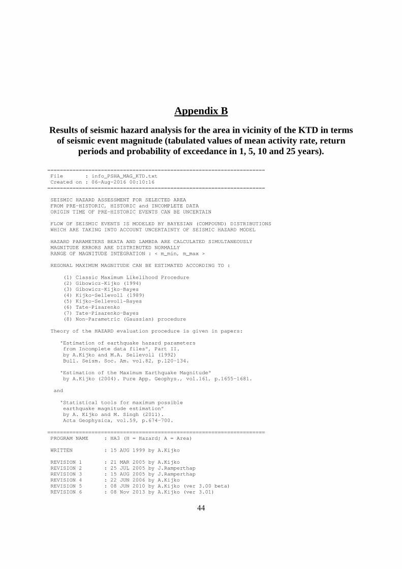
44

Appendix B

Results of seismic hazard analysis for the area in vicinity of the KTD in terms of seismic event magnitude (tabulated values of mean activity rate, return

periods and probability of exceedance in 1, 5, 10 and 25 years). ===================================================================== File : info_PSHA_MAG_KTD.txt Created on : 06-Aug-2016 00:10:16 ===================================================================== SEISMIC HAZARD ASSESSMENT FOR SELECTED AREA FROM PRE-HISTORIC, HISTORIC and INCOMPLETE DATA ORIGIN TIME OF PRE-HISTORIC EVENTS CAN BE UNCERTAIN FLOW OF SEISMIC EVENTS IS MODELED BY BAYESIAN (COMPOUND) DISTRIBUTIONS WHICH ARE TAKING INTO ACCOUNT UNCERTAINTY OF SEISMIC HAZARD MODEL HAZARD PARAMETERS BEATA AND LAMBDA ARE CALCULATED SIMULTANEOUSLY MAGNITUDE ERRORS ARE DISTRIBUTED NORMALLY RANGE OF MAGNITUDE INTEGRATION : < m_min, m_max > REGONAL MAXIMUM MAGNITUDE CAN BE ESTIMATED ACCORDING TO : (1) Classic Maximum Likelihood Procedure (2) Gibowicz-Kijko (1994) (3) Gibowicz-Kijko-Bayes (4) Kijko-Sellevoll (1989) (5) Kijko-Sellevoll-Bayes (6) Tate-Pisarenko (7) Tate-Pisarenko-Bayes (8) Non-Parametric (Gaussian) procedure Theory of the HAZARD evaluation procedure is given in papers: "Estimation of earthquake hazard parameters from Incomplete data files", Part II. by A.Kijko and M.A. Sellevoll (1992) Bull. Seism. Soc. Am. vol.82, p.120-134. "Estimation of the Maximum Earthquake Magnitude" by A.Kijko (2004). Pure App. Geophys., vol.161, p.1655-1681. and "Statistical tools for maximum possible earthquake magnitude estimation" by A. Kijko and M. Singh (2011). Acta Geophysica, vol.59, p.674-700. ===================================================================== PROGRAM NAME : HA3 (H = Hazard; A = Area) WRITTEN : 15 AUG 1999 by A.Kijko REVISION 1 : 21 MAR 2005 by A.Kijko REVISION 2 : 25 JUL 2005 by J.Ramperthap REVISION 3 : 15 AUG 2005 by J.Ramperthap REVISION 4 : 22 JUN 2006 by A.Kijko REVISION 5 : 08 JUN 2010 by A.Kijko (ver 3.00 beta) REVISION 6 : 08 Nov 2013 by A.Kijko (ver 3.01)

45

===================================================================== For more information, contact A.Kijko Natural Hazard Centre, Africa, University of Pretoria, Pretoria 0002, South Africa. E-mail : [email protected] ===================================================================== NAME OF THE AREA: KTD HISTORIC DATA: ******************** NAME OF HISTORIC DATA FILE: e.txt BEGINING OF HISTORIC DATA (Y-M-D) = 1966 5 1 END OF HISTORIC DATA (Y-M-D) = 1971 4 30 NUMBER OF HISTORIC EQ-s = 5 "THRESHOLD" MAG. OF HISTORIC EQ-s = 3.5 STANDARD ERROR OF EQ-e MAGNITUDE = 0.25 1966 7 25 3.8 1968 2 8 3.8 1968 5 3 4.1 1969 5 15 4.3 1970 5 23 5.1 LARGEST EQ IN HISTORIC CATALOG = 5.1 COMPLETE DATA: ******************** NAME OF COMPLETE DATA FILE #1: c_35_mod.txt BEGINING OF COMPLETE DATA #1: 1971 5 1 END OF COMPLETE DATA #1: 2015 2 7 LEVEL OF COMPLETENESS = 3.5 NUMBER OF EQ-s = 591 STANDARD ERROR OF EQ-e MAGNITUDE = 0.15 LARGEST EQ IN COMPLETE CATALOG #1 = 5.4 PROVISION FOR INDUCED SEISMICITY : NOT REQUIRED =============================================== *** TIME SPAN OF WHOLE CATALOG = 48.77 [Y] MAXIMUM MAGNITUDE IN THE CATALOG = 5.4 SE OF MAXIMUM OBSERVED MAGNITUDE = 0.1 MODEL UNCERTAINTY OF BETA = 25 [per cent] MODEL UNCERTAINTY OF LAMBDA = 25 [per cent] CALCULATIONS ARE PERFORMED FOR MINIMUM MAGNITUDE Mmin = 3.50 PRIOR VALUE OF PARAMETER b = 1.25 SD OF PRIOR b-VALUE = 0.1 RESULTS ************* BETA = 2.04 +- 0.10 (b = 0.89 +- 0.04) LAMBDA = 9.320 +- 1.677 (for Mmin = 3.50) Mmax = 5.63 +- 0.11 (for Mmax obs. = 5.40 +- 0.10) Maximum Regional Magnitude Mmax is calculated according to procedure by Kijko-Sellevoll-Bayes COV(Beta,Lambda) = -0.048

46

Mag Lambda RP [Y] Prob(T = 1y 5y 10y 25y) 3.5 9.3199e+000 1.07e-001 0.99935 1.00000 1.00000 1.00000 3.6 7.5735e+000 1.32e-001 0.99797 1.00000 1.00000 1.00000 3.7 6.1635e+000 1.62e-001 0.99456 1.00000 1.00000 1.00000 3.8 5.0220e+000 1.99e-001 0.98732 1.00000 1.00000 1.00000 3.9 4.0954e+000 2.44e-001 0.97392 1.00000 1.00000 1.00000 4.0 3.3415e+000 2.99e-001 0.95191 0.99999 1.00000 1.00000 4.1 2.7264e+000 3.67e-001 0.91934 0.99995 1.00000 1.00000 4.2 2.2235e+000 4.50e-001 0.87532 0.99978 1.00000 1.00000 4.3 1.8113e+000 5.52e-001 0.82020 0.99924 0.99999 1.00000 4.4 1.4727e+000 6.79e-001 0.75556 0.99766 0.99997 1.00000 4.5 1.1938e+000 8.38e-001 0.68380 0.99374 0.99987 1.00000 4.6 9.6374e-001 1.04e+000 0.60774 0.98519 0.99947 1.00000 4.7 7.7347e-001 1.29e+000 0.53015 0.96869 0.99818 1.00000 4.8 6.1578e-001 1.62e+000 0.45350 0.94015 0.99454 0.99998 4.9 4.8484e-001 2.06e+000 0.37976 0.89536 0.98552 0.99988 5.0 3.7589e-001 2.66e+000 0.31033 0.83086 0.96583 0.99938 5.1 2.8506e-001 3.51e+000 0.24614 0.74471 0.92744 0.99724 5.2 2.0918e-001 4.78e+000 0.18765 0.63692 0.85998 0.98916 5.3 1.4568e-001 6.86e+000 0.13500 0.50949 0.75198 0.96242 5.4 9.2440e-002 1.08e+001 0.08805 0.36596 0.59289 0.88451 5.5 4.7719e-002 2.10e+001 0.04653 0.21088 0.37513 0.68355 5.6 1.0088e-002 9.91e+001 0.01003 0.04912 0.09568 0.22139

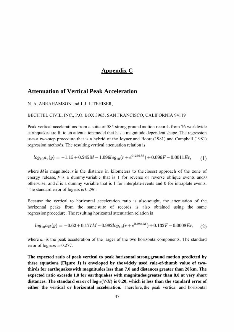
47

Appendix C

Attenuation of Vertical Peak Acceleration

N. A. ABRAHAMSON and J. J. LITEHISER,

BECHTEL CIVIL, INC., P.O. BOX 3965, SAN FRANCISCO, CALIFORNIA 94119

Peak vertical accelerations from a suite of 585 strong ground motion records from 76 worldwide earthquakes are fit to an attenuation model that has a magnitude dependent shape. The regression uses a two-step procedure that is a hybrid of the Joyner and Boore (1981) and Campbell (1981) regression methods. The resulting vertical attenuation relation is

(1)

where M is magnitude, r is the distance in kilometers to the closest approach of the zone of energy release, F is a dummy variable that is 1 for reverse or reverse oblique events and 0 otherwise, and E is a dummy variable that is 1 for interplate events and 0 for intraplate events. The standard error of log10av

is 0.296.

Because the vertical to horizontal acceleration ratio is also sought, the attenuation of the horizontal peaks from the same suite of records is also obtained using the same regression procedure. The resulting horizontal attenuation relation is

(2)

where aH is the peak acceleration of the larger of the two horizontal components. The standard error of log10aH is 0.277.

The expected ratio of peak vertical to peak horizontal strong ground motion predicted by these equations (Figure 1) is enveloped by the widely used rule-of-thumb value of two-thirds for earthquakes with magnitudes less than 7.0 and distances greater than 20 km. The expected ratio exceeds 1.0 for earthquakes with magnitudes greater than 8.0 at very short distances. The standard error of log10(V/H) is 0.20, which is less than the standard error of either the vertical or horizontal acceleration. Therefore, the peak vertical and horizontal

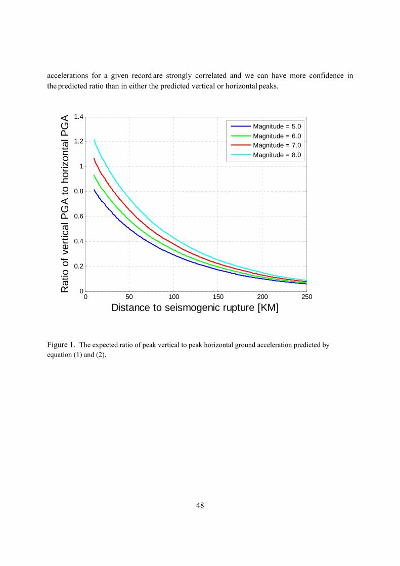
48

accelerations for a given record are strongly correlated and we can have more confidence in the predicted ratio than in either the predicted vertical or horizontal peaks.

Figure 1. The expected ratio of peak vertical to peak horizontal ground acceleration predicted by equation (1) and (2).

0 50 100 150 200 2500

0.2

0.4

0.6

0.8

1

1.2

1.4

Distance to seismogenic rupture [KM]

Ratio o

f vert

ical P

GA

to h

orizonta

l P

GA

Magnitude = 5.0

Magnitude = 6.0

Magnitude = 7.0

Magnitude = 8.0

49

Appendix D

“Introduction to Probabilistic Seismic Hazard Analysis”

Extended version of contribution by A. Kijko to Encyclopedia of Solid Earth

Geophysics, Harsh Gupta (Ed.), Springer, 2011.

Seismic Hazard Encyclopedia of Solid Earth Geophysics Harsh Gupta (Ed.) Springer Prof Andrzej Kijko Pr. Sci. Nat Natural Hazard Centre, Africa Room 4-30, Mineral Sciences Building, University of Pretoria PRETORIA 0002, Republic of South Africa E-mail: [email protected] Tel: +27 12 420 3613 Cell: +27 82 939 4002 Fax: +27 12 362 5219

50

SEISMIC HAZARD Definition Seismic hazard. Any physical phenomena associated with an earthquake (e.g., ground motion, ground failure, liquefaction, and tsunami) and their effects on land, man-made structure and socio-economic systems that have the potential to produce a loss. It is also used without regard to a loss to indicate the probable level of ground shaking occurring at a given point within a certain period of time. Seismic hazard analysis. Quantification of the ground-motion expected at a particular site. Deterministic seismic hazard analysis. Quantification of a single or relatively small number of individual earthquake scenarios. Probabilistic seismic hazard analysis. Quantification of the probability that a specified level of ground motion will be exceeded at least once at a site or in a region during a specified exposure time. Ground motion prediction equation. A mathematical equation which indicates the relative decline of the ground motion parameter as the distance from the earthquake increases. 1. Introduction The estimation of the expected ground motion which can occur at a particular site is vital to the design of important structures such as nuclear power plants, bridges and dams. The process of evaluating the design parameters of earthquake ground motion is called seismic hazard assessment or seismic hazard analysis. Seismologists and earthquake engineers distinguish between seismic hazard and seismic risk assessments in spite of the fact that in everyday usage these two phrases have the same meaning. Seismic hazard is used to characterize the severity of ground motion at a site regardless of the consequences, while the risk refers exclusively to the consequences to human life and property loss resulting from the occurred hazard. Thus, even a strong earthquake can have little risk potential if it is far from human development and infrastructure, while a small seismic event in an unfortunate location may cause extensive damage and losses. Seismic hazard analysis can be performed deterministically, when a particular earthquake scenario is considered, or probabilistically, when likelihood or frequency of specified earthquake size and location are evaluated. The process of deterministic seismic hazard analysis (DSHA) involves the initial assessment of the maximum possible earthquake magnitude for each of the various seismic sources such as active faults or seismic source zones (SSHAC, 1997). An area of up to 450 km radius around the site of interest can be investigated. Assuming that each of these earthquakes will occur at the minimum possible distance from the site, the ground motion is calculated using appropriate attenuation equations. Unfortunately this straightforward and intuitive procedure is overshadowed by the complexity and uncertainty in selecting the appropriate earthquake scenario, creating the need for an alternative, probabilistic methodology, which is free from discrete selection of scenario earthquakes. Probabilistic seismic hazard analysis (PSHA) quantifies as a probability whatever hazard may result from all earthquakes of all possible

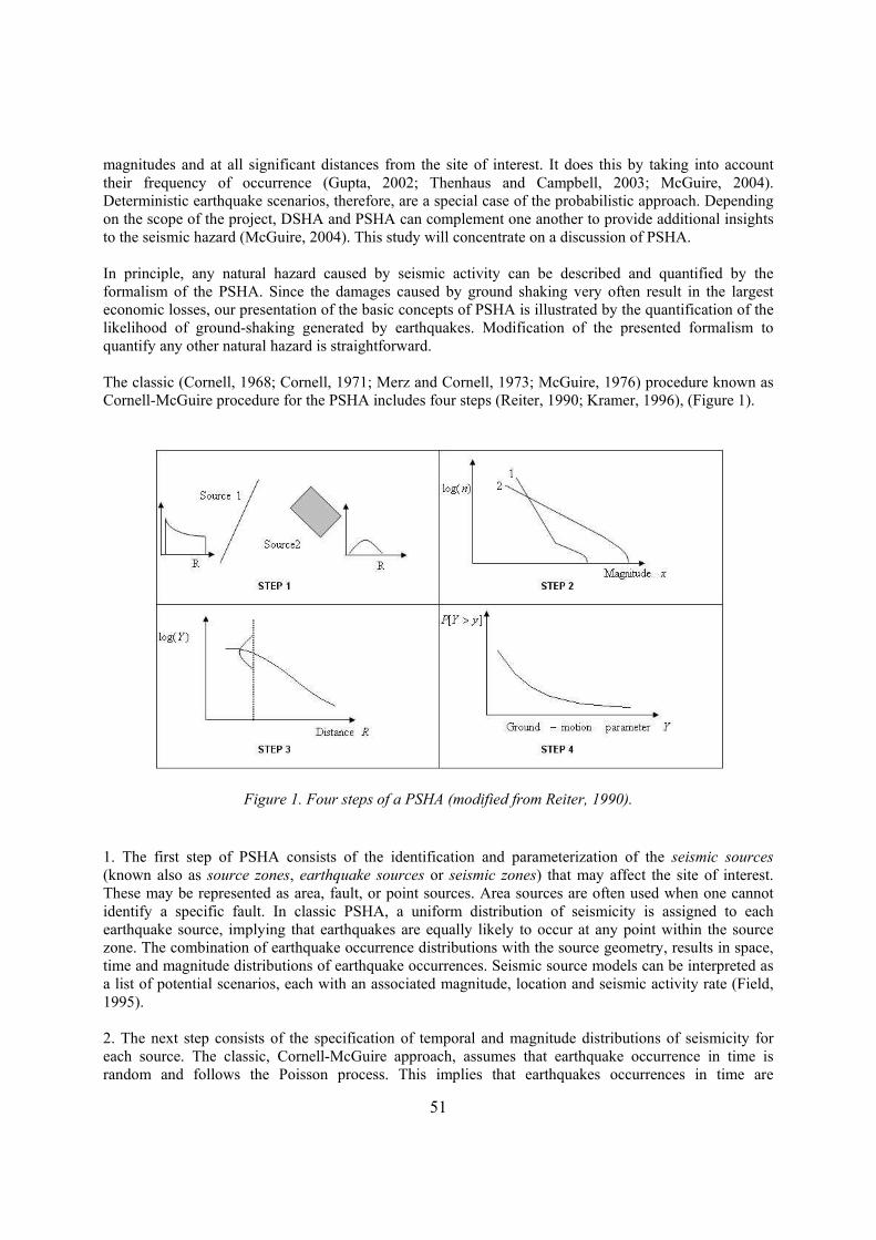
51

magnitudes and at all significant distances from the site of interest. It does this by taking into account their frequency of occurrence (Gupta, 2002; Thenhaus and Campbell, 2003; McGuire, 2004). Deterministic earthquake scenarios, therefore, are a special case of the probabilistic approach. Depending on the scope of the project, DSHA and PSHA can complement one another to provide additional insights to the seismic hazard (McGuire, 2004). This study will concentrate on a discussion of PSHA. In principle, any natural hazard caused by seismic activity can be described and quantified by the formalism of the PSHA. Since the damages caused by ground shaking very often result in the largest economic losses, our presentation of the basic concepts of PSHA is illustrated by the quantification of the likelihood of ground-shaking generated by earthquakes. Modification of the presented formalism to quantify any other natural hazard is straightforward. The classic (Cornell, 1968; Cornell, 1971; Merz and Cornell, 1973; McGuire, 1976) procedure known as Cornell-McGuire procedure for the PSHA includes four steps (Reiter, 1990; Kramer, 1996), (Figure 1).

Figure 1. Four steps of a PSHA (modified from Reiter, 1990). 1. The first step of PSHA consists of the identification and parameterization of the seismic sources (known also as source zones, earthquake sources or seismic zones) that may affect the site of interest. These may be represented as area, fault, or point sources. Area sources are often used when one cannot identify a specific fault. In classic PSHA, a uniform distribution of seismicity is assigned to each earthquake source, implying that earthquakes are equally likely to occur at any point within the source zone. The combination of earthquake occurrence distributions with the source geometry, results in space, time and magnitude distributions of earthquake occurrences. Seismic source models can be interpreted as a list of potential scenarios, each with an associated magnitude, location and seismic activity rate (Field, 1995). 2. The next step consists of the specification of temporal and magnitude distributions of seismicity for each source. The classic, Cornell-McGuire approach, assumes that earthquake occurrence in time is random and follows the Poisson process. This implies that earthquakes occurrences in time are

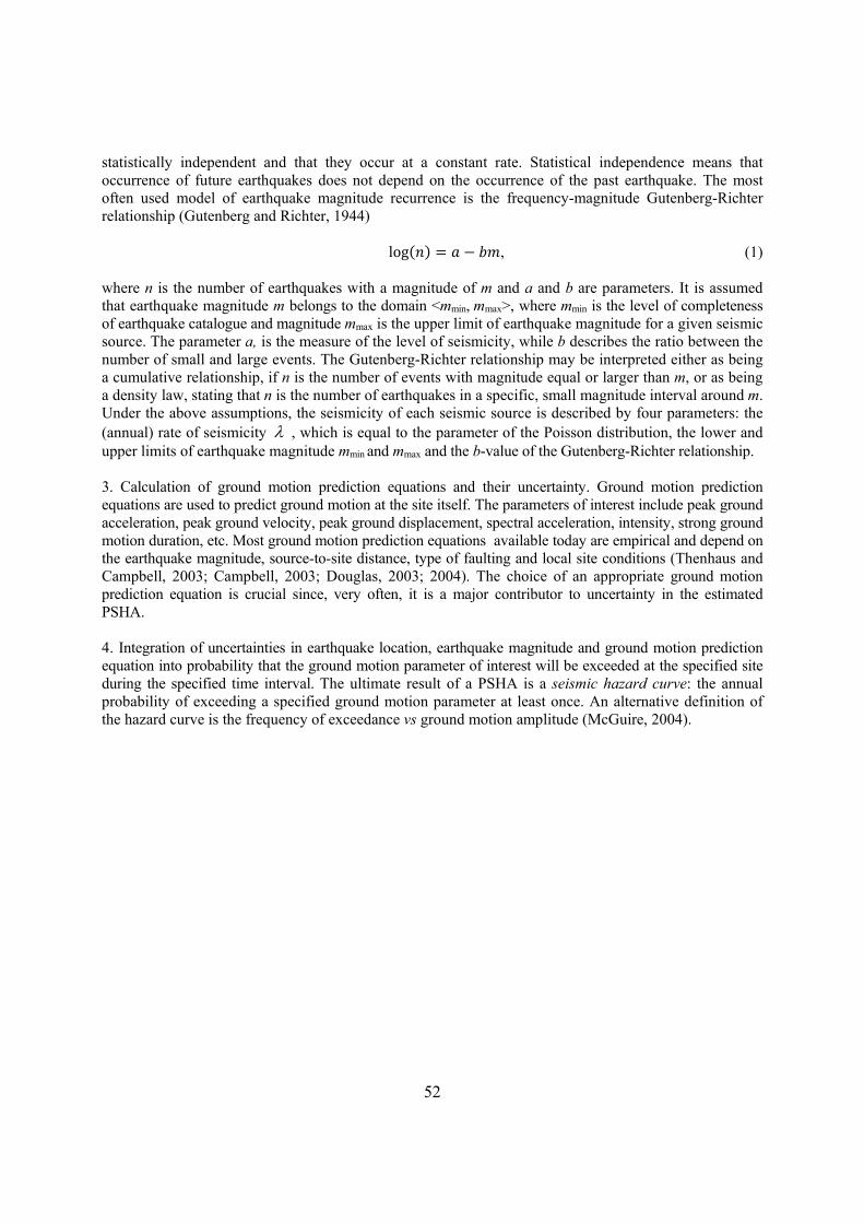
52

statistically independent and that they occur at a constant rate. Statistical independence means that occurrence of future earthquakes does not depend on the occurrence of the past earthquake. The most often used model of earthquake magnitude recurrence is the frequency-magnitude Gutenberg-Richter relationship (Gutenberg and Richter, 1944)

log , (1) where n is the number of earthquakes with a magnitude of m and a and b are parameters. It is assumed that earthquake magnitude m belongs to the domain <mmin, mmax>, where mmin is the level of completeness of earthquake catalogue and magnitude mmax is the upper limit of earthquake magnitude for a given seismic source. The parameter a, is the measure of the level of seismicity, while b describes the ratio between the number of small and large events. The Gutenberg-Richter relationship may be interpreted either as being a cumulative relationship, if n is the number of events with magnitude equal or larger than m, or as being a density law, stating that n is the number of earthquakes in a specific, small magnitude interval around m. Under the above assumptions, the seismicity of each seismic source is described by four parameters: the (annual) rate of seismicity , which is equal to the parameter of the Poisson distribution, the lower and upper limits of earthquake magnitude mmin and mmax and the b-value of the Gutenberg-Richter relationship. 3. Calculation of ground motion prediction equations and their uncertainty. Ground motion prediction equations are used to predict ground motion at the site itself. The parameters of interest include peak ground acceleration, peak ground velocity, peak ground displacement, spectral acceleration, intensity, strong ground motion duration, etc. Most ground motion prediction equations available today are empirical and depend on the earthquake magnitude, source-to-site distance, type of faulting and local site conditions (Thenhaus and Campbell, 2003; Campbell, 2003; Douglas, 2003; 2004). The choice of an appropriate ground motion prediction equation is crucial since, very often, it is a major contributor to uncertainty in the estimated PSHA. 4. Integration of uncertainties in earthquake location, earthquake magnitude and ground motion prediction equation into probability that the ground motion parameter of interest will be exceeded at the specified site during the specified time interval. The ultimate result of a PSHA is a seismic hazard curve: the annual probability of exceeding a specified ground motion parameter at least once. An alternative definition of the hazard curve is the frequency of exceedance vs ground motion amplitude (McGuire, 2004).

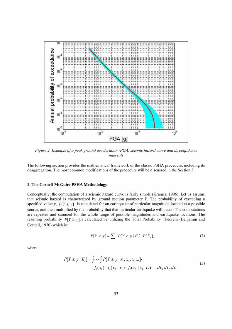
53

Figure 2. Example of a peak ground acceleration (PGA) seismic hazard curve and its confidence intervals

The following section provides the mathematical framework of the classic PSHA procedure, including its deaggregation. The most common modifications of the procedure will be discussed in the Section 3. 2. The Cornell-McGuire PSHA Methodology Conceptually, the computation of a seismic hazard curve is fairly simple (Kramer, 1996). Let us assume that seismic hazard is characterized by ground motion parameter Y. The probability of exceeding a specified value y, ][ yYP , is calculated for an earthquake of particular magnitude located at a possible source, and then multiplied by the probability that that particular earthquake will occur. The computations are repeated and summed for the whole range of possible magnitudes and earthquake locations. The resulting probability ][ yYP is calculated by utilizing the Total Probability Theorem (Benjamin and Cornell, 1970) which is:

],[]|[][ ii EPEyYPyYP (2)

where

....),|()|()(

...],,|[]|[

123213121

321

dxdxdxxxxfxxfxf

xxxyYPEyYP

iii

i

(3)

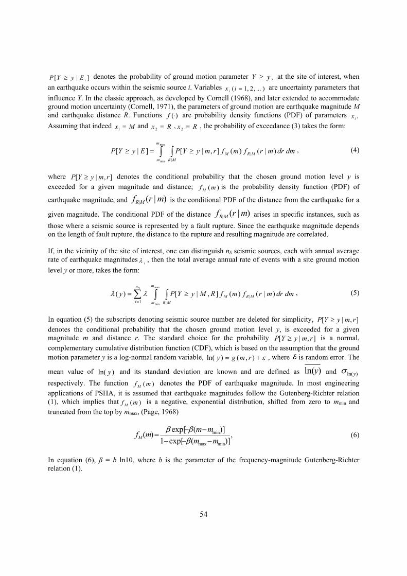
54

]|[ iEyYP denotes the probability of ground motion parameter ,yY at the site of interest, when

an earthquake occurs within the seismic source i. Variables )...,2,1( ix i are uncertainty parameters that

influence Y. In the classic approach, as developed by Cornell (1968), and later extended to accommodate ground motion uncertainty (Cornell, 1971), the parameters of ground motion are earthquake magnitude M and earthquake distance R. Functions )(f are probability density functions (PDF) of parameters .ix

Assuming that indeed Mx 1and Rx 2

, Rx 2, the probability of exceedance (3) takes the form:

MR

MRM

m

m

dmdrmrfmfrmyYPEyYP|

| )|()(],|[]|[max

min

, (4)

where ],|[ rmyYP denotes the conditional probability that the chosen ground motion level y is

exceeded for a given magnitude and distance; )(mf Mis the probability density function (PDF) of

earthquake magnitude, and )|(| mrf MR is the conditional PDF of the distance from the earthquake for a

given magnitude. The conditional PDF of the distance )|(| mrf MR arises in specific instances, such as

those where a seismic source is represented by a fault rupture. Since the earthquake magnitude depends on the length of fault rupture, the distance to the rupture and resulting magnitude are correlated. If, in the vicinity of the site of interest, one can distinguish nS seismic sources, each with annual average rate of earthquake magnitudes

i , then the total average annual rate of events with a site ground motion

level y or more, takes the form:

Sn

i MR

MRM

m

m

dmdrmrfmfRMyYPy1 |

| )|()(],|[)(max

min

, (5)

In equation (5) the subscripts denoting seismic source number are deleted for simplicity, ],|[ rmyYP

denotes the conditional probability that the chosen ground motion level y, is exceeded for a given magnitude m and distance r. The standard choice for the probability ],|[ rmyYP is a normal, complementary cumulative distribution function (CDF), which is based on the assumption that the ground motion parameter y is a log-normal random variable, ),()ln( rmgy , where is random error. The

mean value of )ln( y and its standard deviation are known and are defined as )ln(y and )ln(y

respectively. The function )(mf M denotes the PDF of earthquake magnitude. In most engineering

applications of PSHA, it is assumed that earthquake magnitudes follow the Gutenberg-Richter relation (1), which implies that )(mf M

is a negative, exponential distribution, shifted from zero to mmin and

truncated from the top by mmax, (Page, 1968)

)](exp[1

)](exp[)(

minmax

min

mm

mmmfM

, (6)

In equation (6), β = b ln10, where b is the parameter of the frequency-magnitude Gutenberg-Richter relation (1).

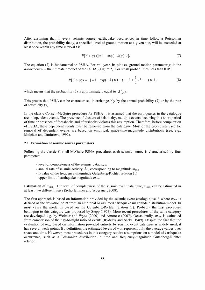
55

After assuming that in every seismic source, earthquake occurrences in time follow a Poissonian distribution, the probability that y, a specified level of ground motion at a given site, will be exceeded at least once within any time interval t is

].)(exp[1];[ tytyYP (7)

The equation (7) is fundamental to PSHA. For t=1 year, its plot vs. ground motion parameter y, is the hazard curve – the ultimate product of the PSHA, (Figure 2). For small probabilities, less than 0.05,

...)2

11(1)exp(1]1;[ 2tyYP , (8)

which means that the probability (7) is approximately equal to )( y .

This proves that PSHA can be characterised interchangeably by the annual probability (7) or by the rate of seismicity (5). In the classic Cornell-McGuire procedure for PSHA it is assumed that the earthquakes in the catalogue are independent events. The presence of clusters of seismicity, multiple events occurring in a short period of time or presence of foreshocks and aftershocks violates this assumption. Therefore, before computation of PSHA, these dependent events must be removed from the catalogue. Most of the procedures used for removal of dependent events are based on empirical, space-time-magnitude distributions (see, e.g., Molchan and Dmitrieva, 1992). 2.1. Estimation of seismic source parameters Following the classic Cornell-McGuire PSHA procedure, each seismic source is characterised by four parameters:

- level of completeness of the seismic data, mmin - annual rate of seismic activity , corresponding to magnitude mmin - b-value of the frequency-magnitude Gutenberg-Richter relation (1) - upper limit of earthquake magnitude mmax

Estimation of mmin. The level of completeness of the seismic event catalogue, mmin, can be estimated in at least two different ways (Schorlemmer and Woessner, 2008). The first approach is based on information provided by the seismic event catalogue itself, where mmin is defined as the deviation point from an empirical or assumed earthquake magnitude distribution model. In most cases the model is based on the Gutenberg-Richter relation (1). Probably the first procedure belonging to this category was proposed by Stepp (1973). More recent procedures of the same category are developed e.g. by Weimer and Wyss (2000) and Amorese (2007). Occasionally, mmin is estimated from comparison of the day-to-night ratio of events (Rydelek and Sacks, 1989). Despite the fact that the evaluation of mmin based on information provided entirely by seismic event catalogue is widely used, it has several weak points. By definition, the estimated levels of mmin represent only the average values over space and time. However, most procedures in this category require assumptions on a model of earthquake occurrence, such as a Poissonian distribution in time and frequency-magnitude Gutenberg-Richter relation.

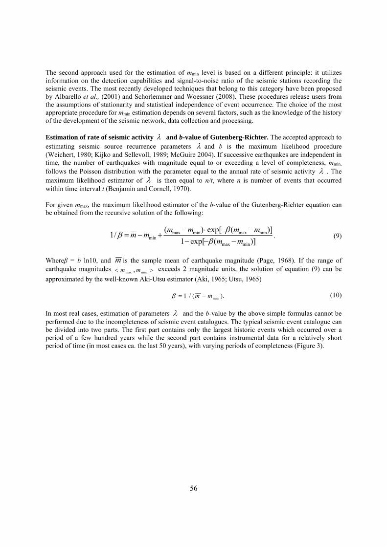
56

The second approach used for the estimation of mmin level is based on a different principle: it utilizes information on the detection capabilities and signal-to-noise ratio of the seismic stations recording the seismic events. The most recently developed techniques that belong to this category have been proposed by Albarello et al., (2001) and Schorlemmer and Woessner (2008). These procedures release users from the assumptions of stationarity and statistical independence of event occurrence. The choice of the most appropriate procedure for mmin estimation depends on several factors, such as the knowledge of the history of the development of the seismic network, data collection and processing. Estimation of rate of seismic activity and b-value of Gutenberg-Richter. The accepted approach to estimating seismic source recurrence parameters and b is the maximum likelihood procedure (Weichert, 1980; Kijko and Sellevoll, 1989; McGuire 2004). If successive earthquakes are independent in time, the number of earthquakes with magnitude equal to or exceeding a level of completeness, mmin, follows the Poisson distribution with the parameter equal to the annual rate of seismic activity . The maximum likelihood estimator of is then equal to n/t, where n is number of events that occurred within time interval t (Benjamin and Cornell, 1970). For given mmax, the maximum likelihood estimator of the b-value of the Gutenberg-Richter equation can be obtained from the recursive solution of the following:

)](exp[1

)](exp[)(/1

minmax

minmaxminmaxmin mm

mmmmmm

. (9)

Whereβ = b ln10, and m is the sample mean of earthquake magnitude (Page, 1968). If the range of earthquake magnitudes minmax , mm exceeds 2 magnitude units, the solution of equation (9) can be

approximated by the well-known Aki-Utsu estimator (Aki, 1965; Utsu, 1965)

).(/1 minmm (10)

In most real cases, estimation of parameters and the b-value by the above simple formulas cannot be performed due to the incompleteness of seismic event catalogues. The typical seismic event catalogue can be divided into two parts. The first part contains only the largest historic events which occurred over a period of a few hundred years while the second part contains instrumental data for a relatively short period of time (in most cases ca. the last 50 years), with varying periods of completeness (Figure 3).

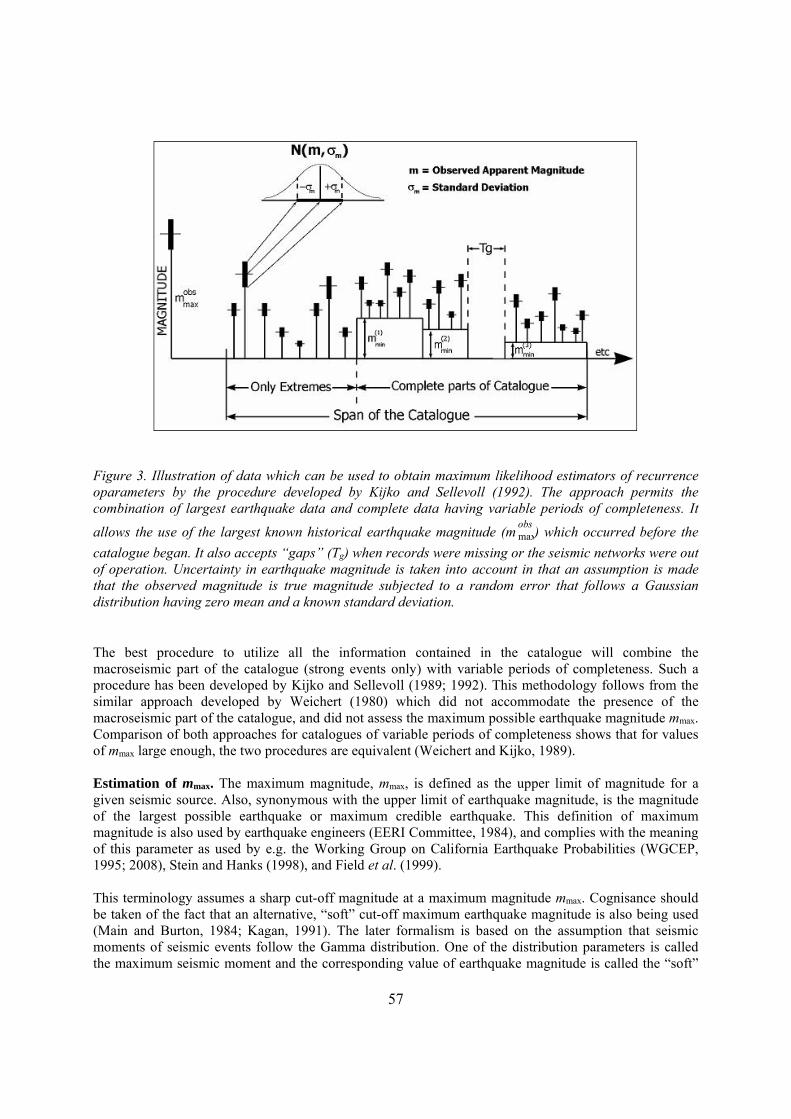
57

Figure 3. Illustration of data which can be used to obtain maximum likelihood estimators of recurrence oparameters by the procedure developed by Kijko and Sellevoll (1992). The approach permits the combination of largest earthquake data and complete data having variable periods of completeness. It

allows the use of the largest known historical earthquake magnitude (mobsmax) which occurred before the

catalogue began. It also accepts “gaps” (Tg) when records were missing or the seismic networks were out of operation. Uncertainty in earthquake magnitude is taken into account in that an assumption is made that the observed magnitude is true magnitude subjected to a random error that follows a Gaussian distribution having zero mean and a known standard deviation. The best procedure to utilize all the information contained in the catalogue will combine the macroseismic part of the catalogue (strong events only) with variable periods of completeness. Such a procedure has been developed by Kijko and Sellevoll (1989; 1992). This methodology follows from the similar approach developed by Weichert (1980) which did not accommodate the presence of the macroseismic part of the catalogue, and did not assess the maximum possible earthquake magnitude mmax. Comparison of both approaches for catalogues of variable periods of completeness shows that for values of mmax large enough, the two procedures are equivalent (Weichert and Kijko, 1989). Estimation of mmax. The maximum magnitude, mmax, is defined as the upper limit of magnitude for a given seismic source. Also, synonymous with the upper limit of earthquake magnitude, is the magnitude of the largest possible earthquake or maximum credible earthquake. This definition of maximum magnitude is also used by earthquake engineers (EERI Committee, 1984), and complies with the meaning of this parameter as used by e.g. the Working Group on California Earthquake Probabilities (WGCEP, 1995; 2008), Stein and Hanks (1998), and Field et al. (1999). This terminology assumes a sharp cut-off magnitude at a maximum magnitude mmax. Cognisance should be taken of the fact that an alternative, “soft” cut-off maximum earthquake magnitude is also being used (Main and Burton, 1984; Kagan, 1991). The later formalism is based on the assumption that seismic moments of seismic events follow the Gamma distribution. One of the distribution parameters is called the maximum seismic moment and the corresponding value of earthquake magnitude is called the “soft”

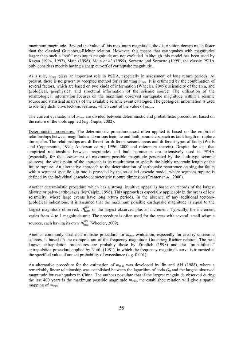
58

maximum magnitude. Beyond the value of this maximum magnitude, the distribution decays much faster than the classical Gutenberg-Richter relation. However, this means that earthquakes with magnitudes larger than such a “soft” maximum magnitude are not excluded. Although this model has been used by Kagan (1994, 1997), Main (1996), Main et al. (1999), Sornette and Sornette (1999), the classic PSHA only considers models having a sharp cut-off of earthquake magnitude. As a rule, mmax plays an important role in PSHA, especially in assessment of long return periods. At present, there is no generally accepted method for estimating mmax. It is estimated by the combination of several factors, which are based on two kinds of information (Wheeler, 2009): seismicity of the area, and geological, geophysical and structural information of the seismic source. The utilization of the seismological information focuses on the maximum observed earthquake magnitude within a seismic source and statistical analysis of the available seismic event catalogue. The geological information is used to identify distinctive tectonic features, which control the value of mmax. The current evaluations of mmax are divided between deterministic and probabilistic procedures, based on the nature of the tools applied (e.g. Gupta, 2002). Deterministic procedures. The deterministic procedure most often applied is based on the empirical relationships between magnitude and various tectonic and fault parameters, such as fault length or rupture dimension. The relationships are different for different seismic areas and different types of faults (Wells and Coppersmith, 1994; Anderson et al., 1996; 2000 and references therein). Despite the fact that empirical relationships between magnitudes and fault parameters are extensively used in PSHA (especially for the assessment of maximum possible magnitude generated by the fault-type seismic sources), the weak point of the approach is its requirement to specify the highly uncertain length of the future rupture. An alternative approach to the determination of earthquake recurrence on singular faults with a segment specific slip rate is provided by the so-called cascade model, where segment rupture is defined by the individual cascade-characteristic rupture dimension (Cramer et al., 2000). Another deterministic procedure which has a strong, intuitive appeal is based on records of the largest historic or paleo-earthquakes (McCalpin, 1996). This approach is especially applicable in the areas of low seismicity, where large events have long return periods. In the absence of any additional tectono-geological indications, it is assumed that the maximum possible earthquake magnitude is equal to the

largest magnitude observed, obsmmax, or the largest observed plus an increment. Typically, the increment

varies from ¼ to 1 magnitude unit. The procedure is often used for the areas with several, small seismic

sources, each having its own obsmmax (Wheeler, 2009).

Another commonly used deterministic procedure for mmax evaluation, especially for area-type seismic sources, is based on the extrapolation of the frequency-magnitude Gutenberg-Richter relation. The best known extrapolation procedures are probably those by Frohlich (1998) and the “probabilistic” extrapolation procedure applied by Nuttli (1981), in which the frequency-magnitude curve is truncated at the specified value of annual probability of exceedance (e.g. 0.001). An alternative procedure for the estimation of mmax was developed by Jin and Aki (1988), where a remarkably linear relationship was established between the logarithm of coda Q0 and the largest observed magnitude for earthquakes in China. The authors postulate that if the largest magnitude observed during the last 400 years is the maximum possible magnitude mmax, the established relation will give a spatial mapping of mmax.

59

Ward (1997) developed a procedure for the estimation of mmax by simulation of the earthquake rupture process. Ward’s computer simulations are impressive; nevertheless, one must realize that all the quantitative assessments are based on the particular rupture model, postulated parameters of the strength and assumed configuration of the faults. The value of mmax can also be estimated from the tectono-geological features like strain rate or the rate of seismic-moment release (Papastamatiou, 1980; Anderson and Luco, 1983; WGCEP, 1995, 2008; Stein and Hanks, 1998; Field et al., 1999). Similar approaches have also been applied in evaluating the maximum possible magnitude of seismic events induced by mining (e.g. McGarr, 1984). However, in most cases, the uncertainty of mmax as determine by any deterministic procedure is large, often reaching a value of the order of one unit on the Richter scale. Probabilistic procedures. The first probabilistic procedure for maximum regional magnitude was developed in the late sixties, and is based on the formalism of the extreme values of random variables. A major breakthrough in the seismological applications of extreme-value statistics was made by Epstein and Lomnitz (1966), who proved that the Gumbel I distribution of extremes can be derived directly from the assumptions that seismic events are generated by a Poisson process and that they follow the frequency-magnitude Gutenberg-Richter relation. Statistical tools required for the estimation of the end-point of distribution functions (as e.g. Tate, 1959; Robson and Whitlock, 1964; Cooke, 1979) have only recently been used in the estimation of maximum earthquake magnitude (Dargahi-Noubary, 1983; Gupta and Trifunac, 1988; Gupta and Deshpande 1994; Pisarenko et al., 1996; Kijko, 2004 and references therein). The statistical tools available for the estimation of mmax vary significantly. The selection of the most suitable procedure depends on the assumptions of the statistical distribution model and/or the information available on past seismicity. Some of the procedures can be applied in the extreme cases when no information about the nature of the earthquake magnitude distribution is available. Some of the procedures can also be used when the earthquake catalogue is incomplete, i.e. when only a limited number of the largest magnitudes are known. Two estimators are presented here. Broadly speaking, the first estimator is straightforward and simple in application, while the second one requires more computational effort but provides more accurate results (Kijko and Graham, 1998). It is assumed that both the analytical form and the parameters of the distribution functions of earthquake magnitude are known. This knowledge can be very approximate, but must be available. Based on the distribution of the largest among n observations (Benjamin and Cornell, 1970), and on the

condition that the largest observed magnitude obsmmax is equal to the largest magnitude to be expected, the

“simple” estimate of mmax is of the form (Pisarenko et al., 1996)

)(

1ˆ

maxmaxmax obs

M

obs

mfnmm , (11)

where )( maxobs

M mf is PDF of the earthquake magnitude distribution. If applied to the Gutenberg-Richter

recurrence relation with PDF (6), it takes the simple form

)](exp[

)](exp[1ˆ

minmax

minmaxmaxmax mmn

mmmm

obs

obsobs

. (12)

The approximate variance of the estimator (12) is of the form

60

,)](exp[

)](exp[11)ˆ(

2

minmax

minmax2

2max

mm

mm

nmVAR

obs

obs

M (13)

where

M stands for epistemic uncertainty and denotes the standard error in the determination of the

largest observed magnitude obsmmax. The second part of the variance represents the aleatory uncertainty of

mmax. The second (“advanced”) procedure often used for assessment of mmax is based on the formalism derived by Cooke (1979)

obsm

m

nM

obs mmFmmmax

min

d)(ˆ maxmax , (14)

where )(mFM

denotes the CDF of random variable m. If applied to the frequency-magnitude Gutenberg-

Richter relation (1), the respective CDF is (Page, 1968)

,for ,1

,for ,)](exp[1

)](exp[1

,for ,0

)(

max

maxminmax

min

min

mm

mmmmm

mm

mm

mF minM

(15)

and the mmax estimator (14) takes the form

),exp()exp(

)()(ˆ min

2

1121maxmax nm

n

nEnEmm obs

(16)

where )]},(exp[1/{ minmax1 mmnn obs )],(exp[ minmax12 mmnn obs and E 1 ( ) denotes an

exponential integral function. The variance of estimator (16) has two components, epistemic and aleatory, and is of the form

2

min2

11212max )exp(

)exp(

)()()ˆ(

nmn

nEnEmVAR M

, (17)

whereM denotes standard error in the determination of the largest observed magnitude

obsmmax.

Both above estimators of mmax, by their nature, are very general and have several attractive properties. They are applicable for a very broad range of magnitude distributions. They may also be used when the exact number of earthquakes, n, is not known. In this case, the number of earthquakes can be replaced by t. Such a replacement is equivalent to the assumption that the number of earthquakes occurring in unit time conforms to a Poisson distribution with parameter , where t is the span of the seismic event

61

catalogue. It is also important to note that both estimators provide a value of maxm̂ , which is never less

than the largest magnitude already observed. Alternative procedures are discussed by Kijko (2004), which are appropriate for the case when the empirical magnitude distribution deviates from the Gutenberg-Richter relation. These procedures assume no specific form of the magnitude distribution or that only a few of the largest magnitudes are known. Despite the fact, that statistical procedures based the mathematical formalism of extreme values provide powerful tools for the evaluation of mmax, they have one weak point: often available seismic event catalogues are too short and insufficient to provide reliable estimations of mmax. Therefore the Bayesian extension of statistical procedures (Cornell, 1994), allowing the inclusion of alternative and independent information such as local geological conditions, tectonic environment, geophysical data, paleo-seismicity, similarity with another seismic area, etc., are able to provide more reliable assessments of mmax. 2.2. Numerical computation of PSHA With the exception of a few special cases (Bender, 1984), the hazard curve (7) cannot be computed analytically. For the most realistic distributions, the integrations can only be evaluated numerically (i.e. Frankel, et al., 1996; Kramer, 1996; Wesson and Perkins, 2001). The common practice is to divide the possible ranges of magnitude and distance into nM and nR intervals respectively. The average annual rate (4) is then estimated as

S M

kj

Rn

i

n

jkRjMkj

n

ki rmrfmfrmyYPyY

1 1 1

)()(],|[)( , (18)

where ,/)()5.0( minmaxmin Mj nmmjmm ,/)()5.0( minmaxmin Rk nrrkrr

,/)( minmax Mnmmm and Rnrrr /)( minmax .

If the procedure is applied to a grid of points, it will result in a map of PSHA, in which the contours of the expected ground motion parameter during the specified time interval can be drawn.

62

Figure 4. Example of product of PSHA. Map of seismic hazard of the world. Peak ground acceleration expected at 10% probability of exceedance at least once in 50 years. (From Giardini, 1999, http://www.gfz-potsdam.de/pb5/pb53/projects/gshap). 2.3. Deaggregation of Seismic Hazard By definition, the PSHA aggregates ground motion contributions from earthquake magnitudes and distances of significance to a site of engineering interest. One has to note that the PSHA results are not representative of a single earthquake. However, an integral part of the design procedure of any critical structure is the analysis of the most relevant earthquake acceleration time series, which are generated by earthquakes, at specific magnitudes and distances. Such earthquakes are called “controlling earthquakes” and they are used to determine the shapes of the response spectral acceleration or PGA at the site. Controlling earthquakes are characterised by mean magnitudes and distances derived from so called deaggregation analysis (e.g. McGuire, 1995; 2004). During the deaggregation procedure, the results of PSHA are separated to determine the dominant magnitudes and the distances that contribute to the hazard curve at a specified (reference) probability. Controlling earthquakes are calculated for different structural frequency vibrations, typically for the fundamental frequency of a structure. In the process of deaggregation, the hazard for a reference probability of exceedance of specified ground motion is portioned into magnitude and distance bins. The relative contribution to the hazard for each bin is calculated. The bins with the largest relative contribution identify those earthquakes that contribute the most to the total seismic hazard.

63

3. Some Modifications of Cornell-McGuire PSHA Procedure and Alternative Models. 3.1. Source-free PSHA procedures. The concept of seismic sources is the core element of the Cornell-McGuire PSHA procedure. Unfortunately, seismic sources or specific faults can often not be identified and mapped and the causes of seismicity are not understood. In these cases, the delineation of seismic sources is highly subjective and is a matter of expert opinion. In addition, often, seismicity within the seismic sources is not distributed uniformly, as it is required by the classic Cornell-McGuire procedure. The difficulties experienced in dealing with seismic sources have stimulated the development of an alternative technique to PSHA, which is free from delineation of seismic sources. One of the first attempts to develop an alternative to the Cornell-McGuire procedure was made by Veneziano et al. (1984). Indeed, the procedure does not require the specification of seismic sources, is non-parametric and as input, requires only information about past seismicity. The empirical distribution of the specified seismic hazard parameter is calculated by using the observed earthquake magnitudes, epicentral distances and assumed ground motion prediction equation. By normalizing this distribution for the duration of the seismic event catalogue, one obtains an annual rate of the exceedance for the required hazard parameter. Another non-parametric PSHA procedure has been developed by Woo (1996). The procedure is also source-free, where seismicity distributions are approximated by data-based kernel functions. Molina at al. (2001) compared the Cornell-McGuire and kernel based procedures and found that the former yields a lower hazard. The kernel based approach has also been used by Jackson and Kagan, (1999) where non-parametric earthquake forecasting is achieved by the computation of the annual rate of seismic activity. Again, the procedure is based exclusively on the seismic event catalogue.

By their nature, the non-parametric procedures work well in areas with a frequent occurrence of strong seismic events and where the record of past seismicity is considerably complete. At the same time, the non-parametric approach has significant weak points. Its primary disadvantage is a poor reliability in estimating small probabilities for areas of low seismicity. The procedure is not recommended for an area where the seismic event catalogues are highly incomplete. In addition, in its present form, the procedure is not capable of making use of any additional geophysical or geological information to supplement the pure seismological data. Therefore, a procedure that accommodates the incompleteness of the seismic event catalogues and, at the same time, does not require the specification of seismic sources, would be an ideal tool for analysing and assessing seismic hazard. Such a procedure, which can be classified as a parametric-historic procedure for PSHA (McGuire, 1993), has been successfully used in several parts of the world. Shepherd et al. (1993) used it for mapping the seismic hazard in El Salvador. The procedure has been applied in selected parts of the world by the Global Seismic Hazard Assessment Program (GSHAP, Giardini, 1999), while Frankel et al. (1996; 2002) applied it for mapping the seismic hazard in the United States. In a series of papers, Frankel and his colleagues modified and substantially extended the original procedure. Their final approach is parametric and based on the assumption that earthquakes within a specified grid size are Poissonian in time, and that the earthquake magnitudes follow the Gutenberg-Richter relation truncated from the top by maximum possible earthquake magnitude mmax. In some cases, the frequency-magnitude Gutenberg-Richter relation is extended by characteristic events. The procedure accepts the contribution of seismicity from active faults and compensates for incompleteness of seismic event catalogues. The final maps of seismic hazard are smoothed by a

64

Gaussian type kernel function. Frankel’s conceptually simple and intuitive parametric-historic approach combines the best of the deductive and non-parametric historic procedures and, in many cases, is free from the disadvantages characteristic of each of the procedures. The rigorous mathematical foundations of the parametric-historic PSHA formalism has been given by Kijko and Graham (1998; 1999) and Kijko (2004). 3.2. Alternative earthquake recurrence models. Time dependent models. In addition to the classic assumption, that earthquake occurrence in time follows a Poisson process, alternative approaches are occasionally used. These procedures attempt to assess temporal, or temporal and spatial dependence of seismicity. Time dependent earthquake occurrence models specify a distribution of the time to the next earthquake, where this distribution depends on the magnitude of the most recent earthquake. In order to incorporate the memory of past events, the non-Poissonian distributions or Markov chains are applied. In this approach, the seismogenic zones that recently produced strong earthquakes become less hazardous than those that did not rupture in recent history. Clearly such models may result in a more realistic PSHA, but most of them are still only research tools and have not yet reached the level of development required by routine engineering applications. An excellent review of such procedures is given by Anagnos and Kiremidjian (1988), Cornell and Winterstein (1988), and by Cornell and Toro (1992). Other more recent treatises of the subject are reviewed e.g. by Muir-Wood (1993) and Boschi et al. (1996). Time dependent occurrence of large earthquakes on segments of active faults is extensively discussed by Rhoades et al. (1994), Ogata (1999), and recently by Faenza et al. (2007). Also, a comprehensive review of all aspects of non-Poissonian models is provided by Kramer (1996). There are several time-dependent models which play an important role in PSHA. The best known models, which have both firm physical and empirical bases, are probably the two models by Shimazaki and Nakata (1980). Based on the correlation of seismic activity with earthquake related coastal uplift in Japan, Shimazaki and Nakata (1980) proposed two models of earthquake occurrence: a time-predictable and a slip-predictable model. The time predictable model states that earthquakes occur when accumulated stress on a fault reaches a critical level, however the stress drop and magnitudes of the subsequent earthquakes vary among seismic cycles. Thus, assuming a constant fault-slip rate, the time to the next earthquake can be estimated from the slip of the previous earthquake. The second, the slip-predictable model, is based on the assumption that, irrespective of the initial stress on the fault, an earthquake occurrence always causes a reduction in stress to the same level. Thus, the fault-slip in the next earthquake can be estimated from the time since the previous earthquake (Shimazaki and Nakata, 1980; Scholz, 1990; Thenhaus and Campbell, 2003). The second group of time-dependent models are less tightly based on the physical considerations of earthquake occurrence, and attempt to describe intervals between the consecutive events by specified statistical distributions. Ogata (1999), after Utsu (1984), considers five models: log-normal, gamma, Weibull, doubly exponential and exponential, which result in the stationary Poisson process. After application of these models to several paleo-earthquake data sets, he concluded that no one of the distributions is consistently the best fit; the quality of the fit strongly depends on the data. From several attempts to describe earthquake time intervals between consecutive events using statistical distributions, at least two play a significant role in the current practice of PSHA: the log-normal model of earthquake occurrence by Nishenko and Buland (1987) and the Brownian passage time (BPT) renewal model by Matthewes et al. (2002).

65

The use of a log-normal model is justified by the discovery that normalized intervals between the consecutive large earthquakes in the circum-Pacific region follow a log-normal distribution with an almost constant standard deviation (Nishenko and Buland, 1987). The finite value for the intrinsic standard deviation is important because it controls the degree of aperiodicity in the occurrence of characteristic earthquakes, making accurate earthquake prediction impossible (Scholz, 1990). Since this discovery, the log-normal model has become a key component of most time-dependant PSHA procedures, and is routinely used by the Working Group on California Earthquake Probabilities (WGCEP, 1995). A time-dependent earthquake occurrence model which is applied more often is the Brownian passage time (BPT) distribution, also known as the inverse Gaussian distribution (Matthewes et al., 2002). The model is described by two parameters: and , which respectively represent the mean time interval

between the consecutive earthquakes and the standard deviation. The aperiodicity of earthquake occurrence, as described by the BPT model, is controlled by the variation coefficient / . For a

small , the aperiodicity of earthquake occurrence is small and the shape of distribution is almost symmetrical. For a large , the shape of distribution is similar to log-normal model, i.e. skewed to the right and peaked at a smaller value than the mean. The straightforward control of aperiodicity of earthquake occurrence, by parameter , makes the BPT model very attractive. It has been used to model earthquake occurrence in many parts of the world and has been applied by the Working Group on California Earthquake Probabilities (1995). Several comparisons of time-dependent with time-independent earthquake occurrence models (Cornell and Winterstein, 1986, Kramer, 1996; Peruzza et al., 2008) have shown that the time-independent (Poissonian) model can be used for most engineering computations of PSHA. The exception to this rule is when the seismic hazard is dominated by a single seismic source, with a significant component of characteristic occurrence when the time interval from the last earthquake exceeds the mean time interval between consecutive events. Note that, in most cases, the information on strong seismic events provided by current databases is insufficient to distinguish between different models. The use of non-Poissonian models will therefore only be justified if more data will be available. Alternative frequency-magnitude models. In the classic Cornell-McGuire procedure for PSHA assessment, it is assumed that earthquake magnitudes follows the Gutenberg-Richter relation truncated from the top by a seismic source characteristic, the maximum possible earthquake magnitude mmax. The PDF of this distribution is given by equation (5). Despite the fact that in many cases the Gutenberg-Richter relation describes magnitude distributions within seismic source zones sufficiently well, there are some instances where it does not apply and the relationship (5) must be modified. In many places, especially for areas of seismic belts and large faults, the Gutenberg-Richter relation underestimates the occurrence of large magnitudes. The continuity of the distribution (5) breaks down. The distribution is adequate only for small events up to magnitude 6.0-7.0. Larger events tend to occur within a relatively narrow range of magnitudes (7.5-8.0) but with a frequency higher than that predicted by the Gutenberg-Richter relation (5). These events are known as characteristic earthquakes (Youngs and Coppersmith, 1985, Figure 5). Often it is assumed that characteristic events follow a truncated Gaussian magnitude distribution (WGCEP, 1995).

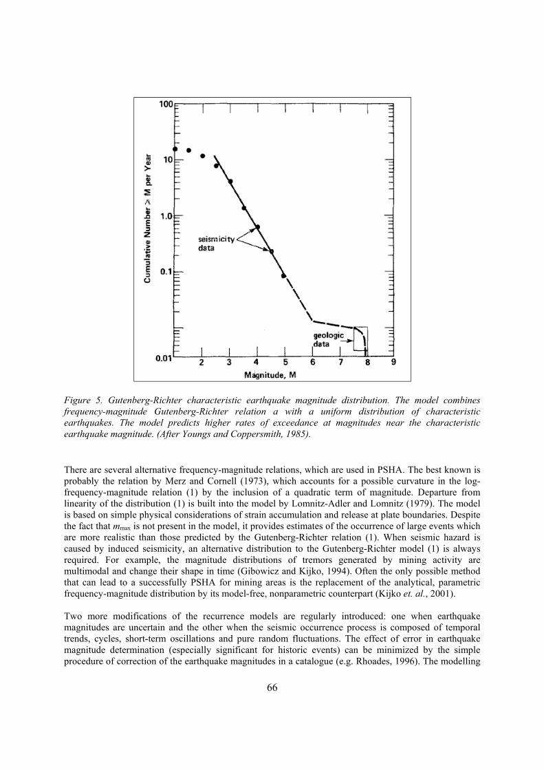
66

Figure 5. Gutenberg-Richter characteristic earthquake magnitude distribution. The model combines frequency-magnitude Gutenberg-Richter relation a with a uniform distribution of characteristic earthquakes. The model predicts higher rates of exceedance at magnitudes near the characteristic earthquake magnitude. (After Youngs and Coppersmith, 1985). There are several alternative frequency-magnitude relations, which are used in PSHA. The best known is probably the relation by Merz and Cornell (1973), which accounts for a possible curvature in the log-frequency-magnitude relation (1) by the inclusion of a quadratic term of magnitude. Departure from linearity of the distribution (1) is built into the model by Lomnitz-Adler and Lomnitz (1979). The model is based on simple physical considerations of strain accumulation and release at plate boundaries. Despite the fact that mmax is not present in the model, it provides estimates of the occurrence of large events which are more realistic than those predicted by the Gutenberg-Richter relation (1). When seismic hazard is caused by induced seismicity, an alternative distribution to the Gutenberg-Richter model (1) is always required. For example, the magnitude distributions of tremors generated by mining activity are multimodal and change their shape in time (Gibowicz and Kijko, 1994). Often the only possible method that can lead to a successfully PSHA for mining areas is the replacement of the analytical, parametric frequency-magnitude distribution by its model-free, nonparametric counterpart (Kijko et. al., 2001). Two more modifications of the recurrence models are regularly introduced: one when earthquake magnitudes are uncertain and the other when the seismic occurrence process is composed of temporal trends, cycles, short-term oscillations and pure random fluctuations. The effect of error in earthquake magnitude determination (especially significant for historic events) can be minimized by the simple procedure of correction of the earthquake magnitudes in a catalogue (e.g. Rhoades, 1996). The modelling

67

of random fluctuations in earthquake occurrence is often done by introducing compound distributions in which parameters of earthquake recurrence models are treated as random variables (Campbell, 1982). 4. Ground Motion Prediction Equations The assessment of seismic hazard at a site requires knowledge of the prediction equation of the particular strong motion parameter, as a function of distance, earthquake magnitude, faulting mechanism and often the local site condition below the site. The most simple and most commonly used form of a prediction equation is

ScFcrcrcmccy 654321 )ln()ln( , (19)

where y is the amplitude of the ground motion parameter (PGA, MM intensity, seismic record duration, spectral acceleration, etc.); m is the earthquake magnitude, r is the shortest earthquake distance from the site to the earthquake source, F is responsible for the faulting mechanism; S is a term describing the site

effect; and is the random error with zero mean and standard deviation )ln(y , which has two

components: epistemic and aleatory. The coefficients

61 ,..., cc are estimated by the least squares or maximum likelihood procedure, using

strong motion data. It has been found that the coefficients depend on the tectonic settings of the site. They are different for sites within stable continental regions, active tectonic regions or subduction zone environments (Thenhaus and Campbell, 2003; Campbell, 2003). Assuming that ln(y) has a normal distribution, regression of (19) provides the mean value of ln(y), the exponent of which corresponds to the median value of y, y

, (Benjamin and Cornell, 1970). Since the log-normal distribution is positively

skewed, the mean value of y, y , exceeds the median value y by a factor of ).5.0exp( 2

)ln(y This

indicates that the seismic hazard for a particular site is higher when expressed in terms of y , than the

hazard for the same site expressed in terms of y . It has been shown that the ground motion prediction

equation remains a particularly important component of PSHA, since its uncertainty is a major contributor to uncertainty of the PSHA results (Bender, 1984; SSHAC, 1997). 5. Uncertainties in PSHA Contemporary PSHA distinguishes between two types of uncertainties, aleatory and epistemic. The aleatory uncertainty is due to randomness in nature; it is the probabilistic uncertainty inherent in any random phenomenon. It represents unique details of any earthquake as its source, path, and site and cannot be quantified before the earthquake occurrence and cannot be reduced by current theories, acquiring addition data or information. It is sometimes referred as “randomness”, “stochastic uncertainty” or “inherent variability” (SSHAC, 1997) and is denoted as UR (McGuire, 2004). The typical examples of aleatory uncertainties are: the number of future earthquakes in a specified area; parameters of future earthquakes such as origin times, epicenter coordinates, depths and their magnitudes; size of the fault rupture; associated stress drop and ground motion parameters like PGA, displacement or seismic record duration at the given site. The aleatory uncertainties are characteristic to the current model and cannot be reduced by the incorporation of addition data. It can only be reduced by the conceptualization of a better model.

68

The epistemic uncertainty, denoted as UK is the uncertainty due to insufficient knowledge about the model or its parameters. The model (in the broad sense of its meaning; as, e.g., a particular statistical distribution etc.) may be approximate and inexact, and therefore predicts values that differ from the observed values by a fixed, but unknown, amount. If uncertainties are associated with numerical values of the parameters, they are also epistemic by nature. Epistemic uncertainty can be reduced by incorporating additional information or data. Epistemic distributions of a model’s parameters can be updated using the Bayes’ theorem. When new information about parameters is significant and accurate, these epistemic distributions of parameters become delta functions about the exact numerical values of the parameters. In such a case, no epistemic uncertainty about the numerical values of the parameters exists and the only remaining uncertainty in the problem is aleatory uncertainty. In the past, epistemic uncertainty has been known as statistical or professional uncertainty (McGuire, 2004). The examples of the epistemic uncertainties are: boundaries of seismic sources, distributions of seismic sources parameters (e.g. annual rate of seismic activity , b-value and mmax), or median value of the ground motion parameter given the source properties. Aleatory uncertainties are included in the PSHA by means of integration over these uncertainties (see eq. 5) and they are represented by the hazard curve. In contrast, epistemic uncertainties are included through the use of an alternative hypothesis - different sets of parameters with different numerical values, different models or through a logic tree. Therefore, by default, if in the process of PSHA, the logic tree formalism is applied, the resulting uncertainties of the hazard curve are of epistemic nature. The major benefit of the separation of uncertainties into aleatory and epistemic is potential guidance in the preparation of input for PSHA and the interpretation of the results. Unfortunately, the division of uncertainties into aleatory and epistemic is model dependent and to a large extent arbitrary, indefinite and confusing (Panel of Seismic hazard Evaluation …, 1997; Toro et al., 1997; Anderson et al., 2000). 6. Logic Tree

The mathematical formalism of PSHA computation, (equation 7 and 9), integrates over all random (aleatory) uncertainties of a particular seismic hazard model. In many cases, however, because of our lack of understanding of the mechanism that controls earthquake generation and wave propagation processes, the best choices for elements of the seismic hazard model is not clear. The uncertainty may originate from the choice of alternative seismic sources, competitive earthquake recurrence models and their parameters as well as from the choice of the most appropriate ground motion. The standard approach for the explicit treatment of alternative hypotheses, models and parameters is the use of a logic tree (Coppersmith and Youngs, 1986). The logic tree formalism provides a convenient tool for quantitative treatment of any alternatives. Each node of the logic tree (Figure 6) represents uncertain assumptions, models or parameters and the branches extending from each node are the discrete uncertainty alternatives (McGuire, 2004).

69

Figure. 6. An example of a simple logic tree. The alternative hypothesis accounts for uncertainty in ground motion attenuation relation, magnitude distribution model and the assigned maximum magnitude mmax. In the logic tree analysis, each branch is weighted according to its probability of being correct. As a result, each end branch represents a hazard curve with an assigned weight, where the sum of weights of all the hazard curves is equal to 1. The derived hazard curves are thus used to compute the final (e.g. mean) hazard curve and their confidence intervals. An example of a logic tree is shown in Figure 6 (Kramer, 1996). The alternative hypotheses account for uncertainty in the ground motion attenuation model, the magnitude distribution model and the assigned maximum magnitude mmax. 7. Controversy Despite the fact that the PSHA procedure, as we know it in its current form, was formulated almost half of century ago, it is not without controversy. The controversy surrounds questions such as: (1) the absence of the upper limit of ground motion parameters, (2) division of uncertainties between aleatory and epistemic, and (3) methodology itself, especially the application of the logic tree formalism. In most currently used Cornell-McGuire based PSHA procedures, the ground motion parameter used to describe the seismic hazard is distributed log-normally. Since the log-normal distribution is unlimited from the top, it results in a nonzero probability of unrealistically high values for the ground motion parameter, e.g., PGA20g, obtained originally from a PSHA for a nuclear-waste repository at Yucca Mountain in the USA (Corradini, 2003). The lack of the upper bound of earthquake-generated ground motion in current hazard assessment procedures has been identified as the “missing piece” of the PSHA procedure (Bommer et al., 2004).

70

Another criticism of the current PSHA procedure concerns portioning of uncertainties into aleatory and epistemic. As noted in Section 5 above, the division between aleatory and epistemic uncertainty remains an open issue. A different criticism comes from the ergodic assumptions which underlie the formalism of the PSHA procedure. The ergodic process is a random process in which the distribution of a random variable in space is the same as distribution of that variable at a single point, when sampled as a function of time (Anderson and Brune, 1999). It has been shown that the major contribution to PSHA uncertainty comes from uncertainty of the ground motion prediction equation. The uncertainty of the ground motion

parameter y, is characterised by its standard deviation, )ln(y , which is calculated as the misfit between

the observed and predicted ground motions at several seismic stations for a small number of recorded earthquakes.

Thus, )ln(y mainly characterises the spatial and not the temporal uncertainty of ground motion at a

single point. This violates the ergodic assumption of the PSHA procedure. According to Anderson and Brune (1999), such violation leads to overestimation of seismic hazard, especially when exposure times are longer than earthquake return times. In addition, Anderson (2000) shows that high-frequency PGA-s observed at short distances do not increase as fast as predicted by most ground motion relations. Therefore the use of the current ground motion prediction equations, especially relating to seismicity recorded at short distances, results in overestimation of the seismic hazard. A similar view has been expressed by Wang and Zhou (2007) and Wang (2009). Inter alia they argue that in the Cornell-McGuire based PSHA procedure, the ground motion variability is not treated correctly. By definition, the ground motion variability is implicitly or explicitly dependent on earthquake magnitude and distance, however, the current PSHA procedure treats it as an independent random variable. The incorrect treatment of ground motion variability results in variability in earthquake magnitudes and distance being counted twice. They conclude that the current PSHA is not consistent with modern earthquake science, is mathematically invalid, can lead to unrealistic hazard estimates and causes confusion. Similar reservations have been expressed in a series of papers by Klügel (see e.g. Klügel, 2007 and references therein) Equally strong criticism of the currently PSHA procedure has been expressed by Castanos and Lomnitz (2002). The main target of their criticism is the logic tree, the key component of the PSHA. They describe the application of the logic tree formalism as a misunderstanding in probability and statistics, since it is fundamentally wrong to admit “expert opinion as evidence on the same level as hard earthquake data”. The science of seismic hazard assessment is thus subject to much debate, especially in the realms where instrumental records of strong earthquakes are missing. At this time, PSHA represents a best-effort approach by our species to quantify an issue where not enough is known to provide definitive results, and by many estimations a great deal more time and measurement will be needed before these issues can be resolved. Further reading: There are several excellent studies that describe all aspects of the modern PSHA. Bommer and Abrahamson (2006) and McGuire (2008) trace the intriguing historical development of PSHA. Hanks and Cornell (1999), and Field (1996) present an entertaining and unconventional summary of the issues related to PSHA, including its misinterpretation. Reiter (1990) comprehensively describes both the deterministic as well as probabilistic seismic hazard procedures from several points of view, including a regulatory perspective. Seismic hazard from the geologist’s perspective is described in the book by Yeats et al., (1997). Kramer (1996) provides an elegant, coherent and understandable description

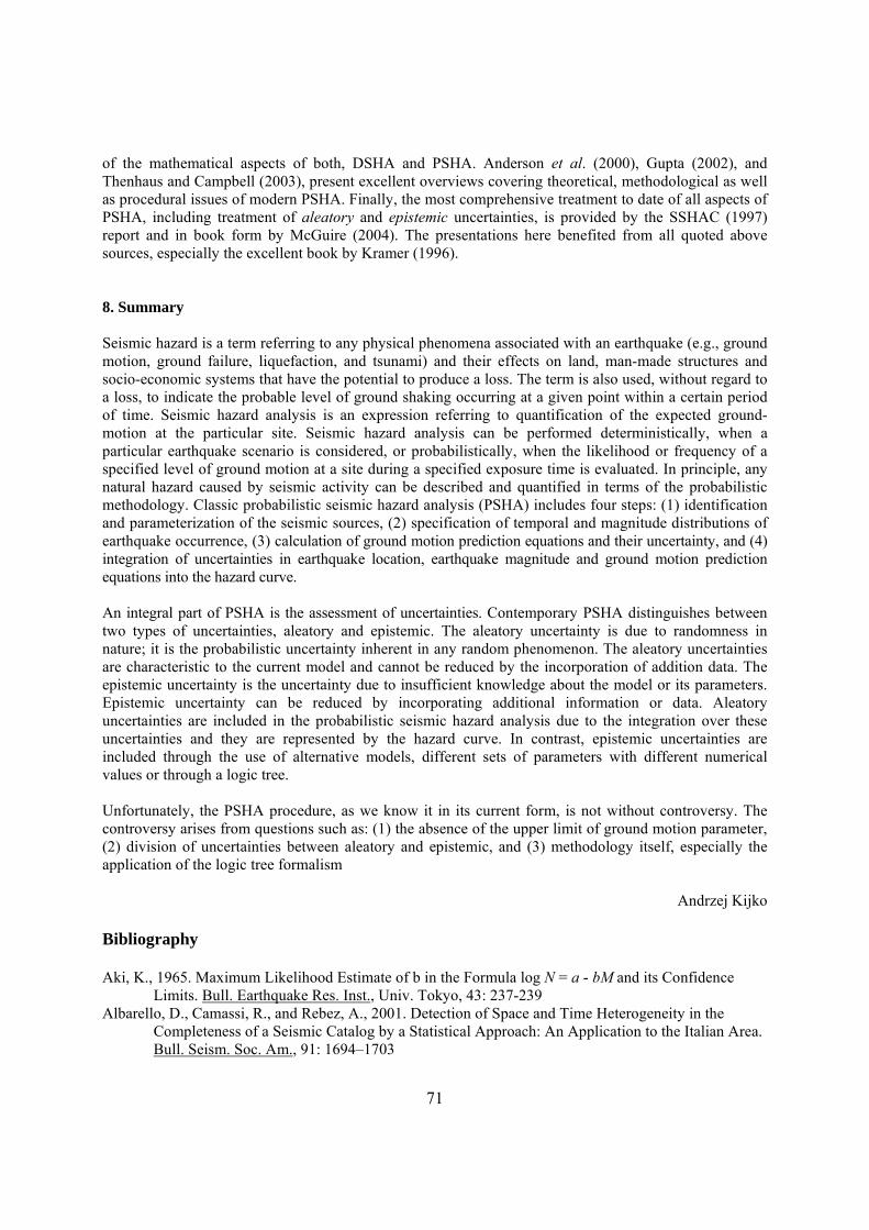
71

of the mathematical aspects of both, DSHA and PSHA. Anderson et al. (2000), Gupta (2002), and Thenhaus and Campbell (2003), present excellent overviews covering theoretical, methodological as well as procedural issues of modern PSHA. Finally, the most comprehensive treatment to date of all aspects of PSHA, including treatment of aleatory and epistemic uncertainties, is provided by the SSHAC (1997) report and in book form by McGuire (2004). The presentations here benefited from all quoted above sources, especially the excellent book by Kramer (1996). 8. Summary Seismic hazard is a term referring to any physical phenomena associated with an earthquake (e.g., ground motion, ground failure, liquefaction, and tsunami) and their effects on land, man-made structures and socio-economic systems that have the potential to produce a loss. The term is also used, without regard to a loss, to indicate the probable level of ground shaking occurring at a given point within a certain period of time. Seismic hazard analysis is an expression referring to quantification of the expected ground-motion at the particular site. Seismic hazard analysis can be performed deterministically, when a particular earthquake scenario is considered, or probabilistically, when the likelihood or frequency of a specified level of ground motion at a site during a specified exposure time is evaluated. In principle, any natural hazard caused by seismic activity can be described and quantified in terms of the probabilistic methodology. Classic probabilistic seismic hazard analysis (PSHA) includes four steps: (1) identification and parameterization of the seismic sources, (2) specification of temporal and magnitude distributions of earthquake occurrence, (3) calculation of ground motion prediction equations and their uncertainty, and (4) integration of uncertainties in earthquake location, earthquake magnitude and ground motion prediction equations into the hazard curve. An integral part of PSHA is the assessment of uncertainties. Contemporary PSHA distinguishes between two types of uncertainties, aleatory and epistemic. The aleatory uncertainty is due to randomness in nature; it is the probabilistic uncertainty inherent in any random phenomenon. The aleatory uncertainties are characteristic to the current model and cannot be reduced by the incorporation of addition data. The epistemic uncertainty is the uncertainty due to insufficient knowledge about the model or its parameters. Epistemic uncertainty can be reduced by incorporating additional information or data. Aleatory uncertainties are included in the probabilistic seismic hazard analysis due to the integration over these uncertainties and they are represented by the hazard curve. In contrast, epistemic uncertainties are included through the use of alternative models, different sets of parameters with different numerical values or through a logic tree. Unfortunately, the PSHA procedure, as we know it in its current form, is not without controversy. The controversy arises from questions such as: (1) the absence of the upper limit of ground motion parameter, (2) division of uncertainties between aleatory and epistemic, and (3) methodology itself, especially the application of the logic tree formalism

Andrzej Kijko

Bibliography Aki, K., 1965. Maximum Likelihood Estimate of b in the Formula log N = a - bM and its Confidence

Limits. Bull. Earthquake Res. Inst., Univ. Tokyo, 43: 237-239 Albarello, D., Camassi, R., and Rebez, A., 2001. Detection of Space and Time Heterogeneity in the

Completeness of a Seismic Catalog by a Statistical Approach: An Application to the Italian Area. Bull. Seism. Soc. Am., 91: 1694–1703

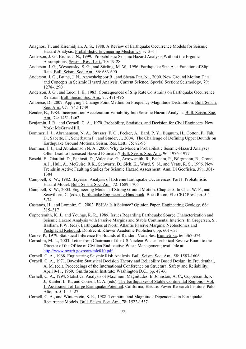
72

Anagnos, T., and Kiremidjian, A. S., 1988. A Review of Earthquake Occurrence Models for Seismic Hazard Analysis. Probabilistic Engineering Mechanics, 3: 3–11

Anderson, J. G., Brune, J. N., 1999. Probabilistic Seismic Hazard Analysis Without the Ergodic Assumptions, Seism. Res. Lett., 70: 19-28

Anderson, J. G., Wesnousky, S. G., and Stirling, M. W., 1996. Earthquake Size As a Function of Slip Rate. Bull. Seism. Soc. Am., 86: 683-690

Anderson, J. G., Brune, J. N., Anooshehpoor R., and Shean-Der, Ni., 2000. New Ground Motion Data and Concepts in Seismic Hazard Analysis. Current Science, Special Section: Seismology, 79: 1278-1290

Anderson, J. G., and Luco, J. E., 1983. Consequences of Slip Rate Constrains on Earthquake Occurrence Relation. Bull. Seism. Soc. Am., 73: 471-496

Amorese, D., 2007. Applying a Change Point Method on Frequency-Magnitude Distribution. Bull. Seism. Soc. Am., 97: 1742-1749

Bender, B., 1984. Incorporation Acceleration Variability Into Seismic Hazard Analysis. Bull. Seism. Soc. Am., 74: 1451-1462

Benjamin, J. R., and Cornell, C. A., 1970. Probability, Statistics, and Decision for Civil Engineers. New York: McGraw-Hill.

Bommer, J. J., Abrahamson, N. A., Strasser, F. O., Pecker, A., Bard, P. Y., Bugnum, H., Cotton, F., Fäh, D., Sabette, F., Scherbaum F., and Studer, J., 2004. The Challenge of Defining Upper Bounds on Earthquake Ground Motions. Seism. Res. Lett., 75: 82-95

Bommer, J. J., and Abrahamson N. A., 2006. Why do Modern Probabilistic Seismic-Hazard Analyses Often Lead to Increased Hazard Estimates? Bull. Seism. Soc. Am., 96: 1976–1977

Boschi, E., Giardini, D., Pantosti, D., Valensise, G., Arrowsmith, R., Basham, P., Bürgmann, R., Crone, A.J., Hull, A., McGuire, R.K., Schwartz, D., Sieh, K., Ward, S. N., and Yeats, R. S., 1996. New Trends in Active Faulting Studies for Seismic Hazard Assessment. Ann. Di Geofisica, 39: 1301-1304

Campbell, K. W., 1982. Bayesian Analysis of Extreme Earthquake Occurrences. Part I. Probabilistic Hazard Model. Bull. Seism. Soc. Am., 72: 1689-1705

Campbell, K. W., 2003. Engineering Models of Strong Ground Motion. Chapter 5. In Chen W. F., and Scawthorn, C. (eds.), Earthquake Engineering Handbook. Boca Raton, FL: CRC Press pp. 5-1 – 5-74.

Castanos, H., and Lomnitz, C., 2002. PSHA: Is it Science? Opinion Paper. Engineering Geology, 66: 315–317

Coppersmith, K. J., and Youngs, R. R., 1989. Issues Regarding Earthquake Source Characterization and Seismic Hazard Analysis with Passive Margins and Stable Continental Interiors. In Gregersen, S., Basham, P.W. (eds), Earthquakes at North Atlantic Passive Margins: Neotectonics and Postglacial Rebound. Dordrecht: Kluwer Academic Publishers, pp. 601-631

Cooke, P., 1979. Statistical Inference for Bounds of Random Variables. Biometrika, 66: 367-374 Corradini, M. L., 2003. Letter from Chairman of the US Nuclear Waste Technical Review Board to the

Director of the Office of Civilian Radioactive Waste Management; available at: http://www.nwtrb.gov/corr/mlc010.pdf

Cornell, C. A., 1968. Engineering Seismic Risk Analysis. Bull. Seism. Soc. Am., 58: 1583-1606 Cornell, C. A., 1971. Bayesian Statistical Decision Theory and Reliability Based Design. In Freudenthal,

A. M. (ed.), Proceedings of the International Conference on Structural Safety and Reliability, April 9-11, 1969. Smithsonian Institute: Washington D.C., pp. 47-66

Cornell, C. A., 1994. Statistical Analysis of Maximum Magnitudes. In Johnston, A. C., Coppersmith, K. J., Kanter, L. R., and Cornell, C. A. (eds), The Earthquakes of Stable Continental Regions - Vol. 1. Assessment of Large Earthquake Potential. California, Electric Power Research Institute, Palo Alto, p. 5–1 - 5–27

Cornell, C. A., and Winterstein, S. R., 1988. Temporal and Magnitude Dependence in Earthquake Recurrence Models. Bull. Seism. Soc. Am., 78: 1522-1537

Documents

WITH ELASTIC MODULUS AND POISSON'S RATIO …