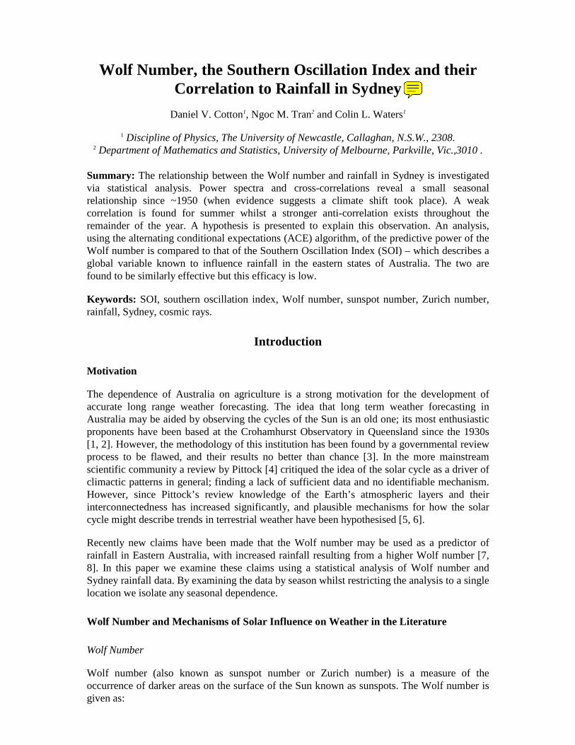
Wolf Number, the Southern Oscillation Index and their Correlation to Rainfall in Sydney

Daniel V. Cotton1, Ngoc M. Tran2 and Colin L. Waters1

1 Discipline of Physics, The University of Newcastle, Callaghan, N.S.W., 2308. 2 Department of Mathematics and Statistics, University of Melbourne, Parkville, Vic.,3010 .

Summary: The relationship between the Wolf number and rainfall in Sydney is investigated via statistical analysis. Power spectra and cross-correlations reveal a small seasonal relationship since ~1950 (when evidence suggests a climate shift took place). A weak correlation is found for summer whilst a stronger anti-correlation exists throughout the remainder of the year. A hypothesis is presented to explain this observation. An analysis, using the alternating conditional expectations (ACE) algorithm, of the predictive power of the Wolf number is compared to that of the Southern Oscillation Index (SOI) – which describes a global variable known to influence rainfall in the eastern states of Australia. The two are found to be similarly effective but this efficacy is low.

Keywords: SOI, southern oscillation index, Wolf number, sunspot number, Zurich number, rainfall, Sydney, cosmic rays.

Introduction

Motivation

The dependence of Australia on agriculture is a strong motivation for the development of accurate long range weather forecasting. The idea that long term weather forecasting in Australia may be aided by observing the cycles of the Sun is an old one; its most enthusiastic proponents have been based at the Crohamhurst Observatory in Queensland since the 1930s [1, 2]. However, the methodology of this institution has been found by a governmental review process to be flawed, and their results no better than chance [3]. In the more mainstream scientific community a review by Pittock [4] critiqued the idea of the solar cycle as a driver of climactic patterns in general; finding a lack of sufficient data and no identifiable mechanism. However, since Pittock’s review knowledge of the Earth’s atmospheric layers and their interconnectedness has increased significantly, and plausible mechanisms for how the solar cycle might describe trends in terrestrial weather have been hypothesised [5, 6].

Recently new claims have been made that the Wolf number may be used as a predictor of rainfall in Eastern Australia, with increased rainfall resulting from a higher Wolf number [7, 8]. In this paper we examine these claims using a statistical analysis of Wolf number and Sydney rainfall data. By examining the data by season whilst restricting the analysis to a single location we isolate any seasonal dependence.

Wolf Number and Mechanisms of Solar Influence on Weather in the Literature

Wolf Number

Wolf number (also known as sunspot number or Zurich number) is a measure of the occurrence of darker areas on the surface of the Sun known as sunspots. The Wolf number is given as:

)10( sgkW += (1)

where s is the number of observable sunspots, g the number of sunspot groups and k a factor to take into account the resolving power of different telescopes. Wolf number varies periodically; its period last century being 10 to 12 years [9]. A high Wolf number is one consequence of increased solar activity. Wolf number is a proxy for the Total Solar Irradiance (TSI), 10.7 cm radio flux etc. The occurrence of brighter spots known as faculae, solar flares and other solar phenomena correlates with sunspot incidence [10].

Solar Forcing by UV

It is known that the variation in total solar irradiance (TSI) over a solar cycle is a mere 0.1%. In isolation, this variation is unable to account for the meteorological phenomena ascribed to it [11, 12]. However, irradiance variation is wavelength dependant; it being greatest for the EUV and the UV [12]. It has been hypothesised that solar forcing of the stratosphere may occur through UV absorption by ozone gases [11]. The portion of the TSI represented by the UV is small. However, ozone concentration varies with UV intensity, resulting in a positive feedback radiative-photochemical mechanism that amplifies the effect of the solar cycle in the lower stratosphere [11].

It has been hypothesised that atmospheric planetary-scale waves provide a mechanism for interaction between the UV absorbing processes in the upper atmosphere and the troposphere, thereby having an effect on terrestrial weather [11]. Coupling between the stratosphere and troposphere is greatest after the Antarctic vortex begins to breakdown in late spring (November), resulting in large anomalies in the Southern Annular Mode (which is related to pressure and sea surface temperature) through summer [11]. This mechanism describes stratospheric anomalies as moving poleward and downward, therefore being most significant for the polar and mid latitudes.

Galactic Cosmic Rays

Galactic Cosmic Rays (GCRs) are composed of very high energy particles accelerated from other stars in our galaxy. The large portion that enter the Earth’s atmosphere participate in nuclear processes that produce secondary particles that penetrate deep into the atmosphere. The ionisation in the atmosphere between 1 km altitude and 35 km altitude is overwhelmingly the result of GCRs [13].

During the peak of solar activity a strong solar flux results in an enhanced interplanetary magnetic field that partially shields the Earth from GCRs [9]. Consequently the flux of GCRs is anti-correlated with Wolf number. The anti-correlation is maximised by introducing an eight month lag [10], since increased solar activity results in a stronger solar flux propagated by the solar wind, which opposes the approach of GCRs from outside the solar system.

It has been suggested that lower atmosphere ionisation caused by GCRs influences cloud formation and changes in cosmic ray flux have been shown to be correlated with cloud cover [13]. One mechanism whereby this could occur involves ion induced formation of aerosol particles from which particle growth results in the formation of cloud condensation nuclei [5].

The Southern Oscillation Index and Weather in Eastern Australia

A global variable known to influence rainfall in the Eastern states of Australia is the southern oscillation, described by the Southern Oscillation Index (SOI) [14, 15]. Comparing the predictive power of the SOI to rainfall with that of the Wolf number provides a measure of statistical significance.

The Southern Oscillation Index

SOI is related to the air pressure difference between Darwin and Tahiti and is given by:

..

.10devstd

avgmonth P

PPSOI

∆∆−∆

= (2)

where ∆P is the pressure difference between Tahiti and Darwin that month (i.e. PTahiti – PDarwin), and the average and standard deviation relate to the complete record of ∆P measurements made since 1915.

Relationship to El Niño

The relationship between the SOI and El Niño weather events is well known [14-16]. Therefore the SOI is one global variable that is correlated with rainfall.

(a)

(b)

(a)

(b)

Fig. 1 (a) The normal circulation pattern results in good rainfall for the eastern states of Australia. (b) The circulation pattern during an El Niño event results in reduced rainfall for

the eastern states of Australia (from [15, 16]).

Normally flows from Antarctic waters result in an up-welling of cold air off the South American coast. A high pressure system moves this air mass across the Pacific to the coast of Australia, where its interaction with warmer waters results in normal rainfall. During an El Niño event the water off the South American coast is warmer than usual and the local air pressure is reduced (creating a negative SOI). Under this condition the easterly trade winds are slowed and can even reverse resulting in reduced rainfall in the eastern Australia [15].

Investigation

Data Acquisition and Processing

Wolf Number

The daily sunspot number (i.e. Wolf number) was obtained from the Solar Influences Data Analysis Centre (SIDC) website [17]. Monthly values were obtained by averaging the daily data over a calendar month. Seasonal values were obtained by averaging the three months that make up a season – summer: December (previous year), January, February; autumn: March, April, May; winter: June, July, August; spring: September, October, November.

Sydney Rainfall

Australian daily rainfall data was obtained from the Australian Government Bureau of Meteorology National Climate Centre [18]. The quantity termed ‘Sydney rainfall’ in this paper is an average of data obtained from several Australian Bureau of Meteorology rainfall stations in the Sydney metropolitan area. The data were averaged to eliminate anomalies peculiar to any one station and account for lack of continuous data at some sites. The stations were Sydney Airport AMO (#66037), Mosman (Bapaume Road) (#66042), Sydney (Observatory Hill) (#66062), Wollstonecraft (#66067), Randwick Racecourse (#66073) and Centennial Park (#66160). A station is included in the average only if there is sufficient data for the duration of interest. The monthly rainfall for a particular station was computed as the total rainfall for the month where there were at least 27 days of available data. The seasonal average rainfall was calculated as the average of monthly rainfall for each of the months in the season where there were three sufficiently complete months of data available.

2km

Mosman

Wollstonecraft

Observatory Hill

AshfieldCentennial Pk.

Randwick

Airport

Map of Sydney Rainfall Stations Utilised

2km

Mosman

Wollstonecraft

Observatory Hill

AshfieldCentennial Pk.

Randwick

Airport

Map of Sydney Rainfall Stations Utilised

Fig. 2 Sydney rainfall is an average of available data from seven rainfall stations (map information obtained from [19]).

Southern Oscillation Index

The Southern Oscillation Index (SOI) data were also obtained from the Australian Government Bureau of Meteorology National Climate Centre [16]. SOI data is provided with a one month resolution. Seasonal average SOI values were obtained by averaging the three months that make up each season.

Evidence for a climate shift

Time Series

— monthly average— 3y moving average

— 1y moving average— 3y moving average

— monthly SOI— 1y moving average

(a)

(b)

(c)

— monthly average— 3y moving average

— 1y moving average— 3y moving average

— monthly SOI— 1y moving average

(a)

(b)

(c)

Fig. 3 Time series of the data used in this investigation (1915-2005) for (a) Wolf number, (b) rainfall in Sydney and (c) the southern oscillation index.

Upon inspection of the Sydney rainfall time series it was noticed that there was a marked difference in long term variation beginning around 1950. This was quite unexpected. Consequently the data analysis included a separation of pre- and post-1950 data. It should be noted that this phenomenon was not restricted to Sydney, preliminary investigation revealed similar trends in other regions of eastern Australia.

Power Spectra

Power spectra of the rainfall data confirms the presence of strong long period character post-1950 not present in the first half of the century. Particularly noteworthy is that the rainfall period displayed post-1950 is approximately 11 years – very close to the period in the Wolf number. A similar analysis of the SOI also reveals a different long period character pre- and post-1950. The SOI is not thought to be linked to solar activity [13], and indeed there is no 10 or 11 year period in either the pre- or post-1950 SOI data. The fact that there is a change in two different measures of the weather suggests a shift into a different climate regime. It seems plausible that such a shift could result in a system more sensitive to solar influences.

Fig. 4 Power spectra of (left) Sydney rainfall and (right) SOI, revealing a distinct change in the long period character of each pre/post the middle of the 20th century. (top) The Wolf

number is shown for comparison (the period of which is ~ static over the same duration [9]).

Kolmogorov-Smirnov Test

A statistical basis for the conclusion of climate shift around 1950 was obtained by applying the Kolmogorov-Smirnov (K-S) test to both Sydney rainfall and the SOI data. The K-S test compares the cumulative distribution functions of two series in terms of a D-statistic to gauge their likeness [20]. The D-statistic for the simple case of two equally sized distributions is given by:

)()(max

21xSxS

xD NN −

∞<<∞−= (3)

where SN(x) is the xth ordered element in the cumulative sum of population N. Appropriate scaling is applied for two unequally sized distributions. The null hypothesis is that the pre- and post-1950 time series are from the same distribution. A large D-statistic indicates the series are unalike; the smaller the D-statistic the less likely the two distributions are different. QKS is the probability that the null hypothesis is correct [20].

The K-S test shows that rainfall is significantly different over the two durations. When the SOI is smoothed with a 1-year moving average to remove low frequency noise and bias the test to longer term trends, it too is significantly different, supporting the climate shift conclusion.

Table 1 Results of the K-S test for distributions pre- and post-1950.

K-S Test

statistic D QKS D QKS

Sydney rainfall 0.095 0.63% 0.210 0.00%

SOI 0.065 20.00% 0.110 0.22%

Monthly 1y Moving Average

Having established the occurrence of a climate shift around 1950, since we are interested in solar influences and the rainfall data post 1950 has a peak in the power spectra of ~11 years, and noting that the influence of SOI on rainfall in eastern Australia has been established for this period [14, 21] we concentrate on analysis of the period 1951-2005 for the remainder of the paper.

Wolf number and rainfall (1951-2005)

Power Spectra

Evidence for an ~11 year period in rainfall data (1951-2005) is present in the power spectra. When the analysis is binned by season the 11 year period is most prominent for winter and then autumn. The 11 year peak is still present in spring but is weaker, yet no such period can be seen in summer. This implies that, if the 11 year period is indeed due to a solar cycle influence on rainfall, that the effect is seasonal – being strongest in winter.

Cross-Correlation

The cross-correlation of Wolf number with Sydney rainfall plotted against the lag of the two data sets (shown in the top panel of Fig. 5(b)) reveals an interesting pattern; there is a peak in anti-correlation that is lagged by approximately one year. An anti-correlation between Wolf number and rainfall suggests that GCRs might be responsible for increased rainfall, where logically the ~1 year lag, by its correspondence to the eight month lag between Wolf number and GCR flux maxima reported in the literature [10], reinforces this argument. However, the value of the correlation coefficient is low, such that ordinarily the anti-correlation would be dismissed as insignificant. This notwithstanding, when the analysis is binned by season the maximum correlation in winter exceeds 0.4, and 0.2 in autumn and spring. Those three seasons’ rainfall are roughly anti-correlated with Wolf number, in summer Wolf number and Sydney rainfall are weakly correlated.

Presuming that winter (and to a lesser extent autumn and spring) rainfall in Sydney is influenced by GCRs then we might inquire as to why this is not the case in summer. We note that local climatic conditions such as severe convective summer storms [22] may dominate seasonal rainfall trends. However, comparing each season separately as we have done should allow the influence of global variables to be detected. One hypothesis to explain the contrary trend in summer involves solar forcing by UV. As mentioned previously, the Antarctic vortex begins to break down in late spring, providing a mechanism for coupling between the stratosphere and troposphere which is present throughout summer. The increased output of solar UV during solar maximum would then counter the increased GCR flux at solar minimum, from late spring through summer. This hypothesis has the further benefit of explaining the shifting lags for maximum correlation of the different seasons. Because there is an eight month offset between the maximum of GCR flux and Solar minimum, an altered ratio

of the influence of the two competing mechanisms will shift the maximum of the correlation between rainfall and Wolf number toward the trend of the increased mechanism. For example; say in winter that the only influence on rainfall was GCR flux, then the cross-correlation versus lag plot for rainfall and Wolf number would be anti-correlated with an eight month lag. When the season changes to spring, GCR flux still contributes the same effect but now the effects of solar UV begin to be felt and are superimposed with those of the GCRs, resulting in a smoothing out of the plot and a shift of the maximum correlation peak back towards zero years. Furthermore, if each of these two mechanisms operate on the system then we would expect a peak in the power spectrum corresponding to approximately half the period of the solar cycle (as increased rainfall would occur as a result of GCR flux maximum and solar UV maximum). Such a peak is prominent in spring and might also be argued for in autumn.

Power Spectra: Sydney(1951-2005)(a) (b)

Power Spectra: Sydney(1951-2005)(a) (b)

Power Spectra: Sydney(1951-2005)Power Spectra: Sydney(1951-2005)(a) (b)

Fig. 5 (a) Power spectra of Sydney rainfall, the dashed line indicates an 11 year period (approximately that of the Wolf number). (b) Cross-correlation of Sydney rainfall with Wolf number. Dashed lines indicate approximate values of (grey and black) Wolf number maxima,

(pink) cosmic ray minimum and (red) cosmic ray maximum. Both the power spectra and cross-correlation analysis were conducted for the full year (top) and for summer (yellow),

autumn (orange), winter (grey) and spring (green) in isolation.

Comparison of Wolf Number with SOI for Rainfall Prediction

Alternating Conditional Expectations Algorithm

The alternating conditional expectations (ACE) algorithm transforms response and predictor variables to any functional form to produce the maximal linear effect between them [23]. A representative example is presented in Fig. 6. The transformations of three individual data points are traced out with the pink, fuchsia and red lines. Notice that the maximum rainfall corresponds to a lower Wolf number (red line). ACE analysis allows the use of one or more predictor variables and R2 indicates the ability of the variable(s) to predict the response. Note that √( R2) compares to the correlation coefficient.

200 150 100 50 0-2

-1

0

1

2

3

4

1.5

1.0

0.5

0.0

-0.5

-1.0

-1.5 -1.0 -0.5 0.0 0.5 1.0 1.5 2.0

-1.5 -1.0 -0.5 0.0 0.5 1.0 1.5 2.0-2

-1

0

1

2

3

4

200 150 100 50 0

1.5

1.0

0.5

0.0

-0.5

-1.0

ACE:Sydney(1951-2005)

Autumn

Sta

ndar

dise

d M

onth

ly R

ainf

all

Wolf Number Transformation(Rainfall)

Tra

nsfo

rmat

ion(

Wol

f Num

ber)

Fig. 6 The ACE transformation for Wolf number and Sydney rainfall for autumn (1951-2005).

Comparison between SOI and Wolf number as Rainfall Predictors

Wolf number and SOI are used as predictors for rainfall in the ACE analysis. The previous season’s SOI and Wolf number are used to predict rainfall following the suggestion made by Russell et al. [14].

Fig. 7 reveals R2 values for Wolf number around 0.3, and typically lower values for the SOI. For a global variable an R2 value of around 0.4 would be quite significant [14], 0.3 is on the low side, but is perhaps not insignificant. The lower panel in Fig. 7 shows the 95% confidence interval range of the slope between the ACE determined transformed predictor and transformed response variables. The important point to note from the confidence intervals in

Fig. 7 is whether or not they pass through zero, as zero would indicate no relationship. In all but one instance the results are shown to be significant to the 95% confidence level. Curiously, given the high correlation coefficient, Wolf number as predictor for winter rainfall does not pass this test. Furthermore, winter is the only season where the SOI is the better predictor. This analysis reveals that SOI is not as good a predictor of rainfall in Sydney as in areas further North studied by Russell [14]. It also indicates that SOI is a better predictor for the winter than summer which is unusual for eastern Australia.

0

1

2

3

95

%

Co

nf

id

en

ce

I

nt

er

va

l

Ra

ng

e

ACE: Predictors for Sydney Rainfall 1951-2005

00.10.20.30.40.50.6

Summer Autumn Winter Spring

R2

SOI

Wolf Number

Both

1

2

0

Ran

ge

95% Confidence Intervals3

0

1

2

3

95

%

Co

nf

id

en

ce

I

nt

er

va

l

Ra

ng

e

ACE: Predictors for Sydney Rainfall 1951-2005

00.10.20.30.40.50.6

Summer Autumn Winter Spring

R2

SOI

Wolf Number

Both

1

2

0

Ran

ge

95% Confidence Intervals3

Fig. 7 ACE analysis results showing the (top) R2 and (bottom) confidence intervals for the predictors of Sydney rainfall between 1951 and 2005 by season.

ACE: Predictors for Sydney Rainfall 1915-1950

00.10.20.30.40.50.6

Summer Autumn Winter Spring

R2

SOI

Wolf Number

Both

0 . 0

0 . 5

1 . 0

1 . 5

2 . 0

2 . 5

1

2

0

Ran

ge

95% Confidence Intervals2.5

1.5

0.5

ACE: Predictors for Sydney Rainfall 1915-1950

00.10.20.30.40.50.6

Summer Autumn Winter Spring

R2

SOI

Wolf Number

Both

0 . 0

0 . 5

1 . 0

1 . 5

2 . 0

2 . 5

1

2

0

Ran

ge

95% Confidence Intervals2.5

1.5

0.5

Fig. 8 ACE analysis results showing the (top) R2 and (bottom) confidence intervals for the predictors of Sydney rainfall between 1915 and 1950 by season.

Compared to 1951-2005, the period 1915-1950 produces smaller R2 values and wider confidence intervals with Wolf number as the predictor. The exception is winter where the analysis produces an R2 value of ~0.45 with a narrow 95% confidence interval not passing

through zero. The result for winter is in line with what we would have expected from the later time period also, where GCR flux, undiluted by the influence of solar UV, produces a stronger relationship between Wolf number and Sydney rainfall than in the other seasons. Hence, in terms of the hypothesis discussed earlier, the ACE result for winter (1951-2005) is anomalous. In general the SOI R2 values are also lower than those for the latter period, indicating that a result of the climate shift has been that rainfall is more sensitive to the SOI (a result consistent with that of McBride and Nicholls [21]), and seemingly also Wolf number.

The ACE analysis indicates that in general Wolf number is a better predictor of Sydney rainfall than the southern oscillation index. Given that the SOI is a global variable that is known to predict rainfall in eastern Australia, this result would indicate that the Wolf number should also be considered a predictor. However, the low R2 values for SOI in particular, suggests that neither predictor is particularly reliable. Therefore, the result is promising but ultimately inconclusive.

Conclusions

The K-S test suggests that weather patterns shifted into the present regime around 1950. Since 1950 the Sydney rainfall data show a prominent long period character with a period of ~11 years. Pre and post 1950, the SOI spectra also has a difference in (long period) periodicity as shown by the power spectrum analysis; the K-S result is corroborative.

Power spectra by season reveal the presence of an ~11 year period in rainfall data in autumn, winter and spring; this is similar to the period of the Wolf number. Cross-correlations of rainfall with Wolf number reveal a weak correlation in Summer and a rough anti-correlation during the other seasons. Therefore, the power spectra and cross-correlations for Autumn, Winter and Spring are consistent with increased rainfall in Sydney during periods of high GCR flux (the opposite of the claim made by Baker [8]). Although there is no prominent 11 year peak in the power spectrum of summer rainfall, the cross-correlation displays a weak correlation for lags of ~0 and ~11 years. Wolf number correlation with rainfall in Summer suggests a link between the two, maybe via a solar UV forcing mechanism that couples into the troposphere during Antarctic vortex breakdown. It is worth noting that the combination of mechanisms proposed would not be apparent if the analysis had been binned by year. Only by binning the data by season were the observed patterns apparent. Therefore, a recommendation from this work is that future analyses consider seasonal dependence.

In general, ACE analysis reveals that the Wolf number and SOI are better predictors of Sydney rainfall after 1950, although neither are good predictors. ACE analysis using Wolf number and SOI as predictors reveals that the two predictors are comparable in efficacy. In fact the Wolf number is often a better predictor than the SOI. The confidence intervals in all but one case do not contain zero. However, R2 values are generally on the low side, and so it is not possible to come to a definitive conclusion with regard to the influence of the Wolf number. A more satisfying result might be achieved by using records of GCR flux in addition to Wolf number as predictors.

Acknowledgements

The authors wish to thank Dr. Steven Morley for some useful discussions.

References

[1] I. Jones, "The Crohamhurst Observatory: it's location and functions and the inaugural ceremony," Crohamhurst Paper, vol. 1, pp. 1-16, 1935.

[2] I. Jones, "Long range weather forecasting," Qld. Geograph. J., pp. 80-105, 1943. [3] "Report of the Committee appointed to enquire into the forecasting system of Mr Inigo

Jones of Crohamhurst (Queensland)," Queensland Government NAA: A431, 1953/591, 1940.

[4] A. B. Pittock, "Critical look at long-term sun-weather relationships," Rev. Geophys. Space Phys., vol. 16, pp. 400-420, 1978.

[5] F. Arnold, "Atmospheric aerosol and cloud condensation nuclei formation: a possible influence of cosmic rays?," Space Sci. Rev., vol. 125, pp. 169-186, 2006.

[6] M. A. Geller, "Discussions of the solar UV/planetary wave mechanism: introductory paper," Space Sci. Rev., vol. 125, pp. 337-246, 2006.

[7] UNE Media Release, "Sunspot cycles a key to drought prediction," Australian Physics, vol. 43, pp. 78, 2006.

[8] M. Warren, "Sun's pulses point to drenching rain," in The Australian, 2007. [9] M. Fligge, S. K. Solanki, and J. Beer, "Determination of solar cycle length variations

using continuous wavelet transform," Astron. Astrophys., vol. 346, pp. 313-321, 1999. [10] D. H. Hathaway and R. M. Wilson, "What the sunspot record tells us about space

climate," Sol. Phys., vol. 224, pp. 5-19, 2005. [11] M. P. Baldwin and T. J. Dunkerton, "The solar cycle and stratosphere-troposphere

dynamic coupling," J. Atmos. Sol-Terr. Phys., vol. 67, pp. 71-82, 2005. [12] C. Fröhlich and J. Lean, "Solar radiative output and its variability: evidence and

mechanisms," The Astron. Astrophys. Rev., vol. 12, pp. 273-320, 2004. [13] H. Svensmark, "Cosmic rays and Earth's climate," Space Sci. Rev., vol. 93, pp. 175-

185, 2000. [14] J. S. Russell, I. M. McLeod, M. B. Dale, and T. R. Valentine, "The Southern

Oscillation Index as a predictor of seasonal rainfall in the arable areas of the inland Australian subtropics," Aust. J. Agric. Res., vol. 44, pp. 1337-1349, 1993.

[15] G. Youngberry, NBN Weather Book, 2006. [16] "Australian Government Bureau of Meteorology National Climate Centre Website

(http://www.bom.gov.au/)," obtained online 1/3/2007. [17] "SIDC – Solar Influences Data Analysis Centre (http://sidc.oma.be/)," obtained online

1/9/2006. [18] "Australian Daily Rainfall (IDCJDCO3.200606)," Australian Government Bureau of

Meteorology National Climate Centre, June 2006, pp. DVD ROM. [19] "Google Maps (http://maps.google.com)," obtained online 1/2/2007. [20] W. H. Press, S. A. Teukolsky, W. T. Vetterling, and B. P. Flannery, Numerical Recipes

in FORTRAN, 2nd ed., U.S.A.: Cambridge University Press, 1992. [21] J. L. McBride and N. Nicholls, "Seasonal Relationships between Australian Rainfall

and the Southern Oscillation," Mon. Weather Rev., vol. 111, pp. 1998-2004, 1983. [22] M. S. Speer, L. M. Leslie, and L. Qi, "Numerical prediction of severe convection:

comparison with operational forecasts," Meteorol. Appl., vol. 10, pp. 11-19, 2003. [23] D. Wang and M. Murphy, "Estimating optimal transformations for multiple regression

using the ACE algorithm," J. Data Sci., vol. 2, pp. 329-246, 2004.