Women and Stability: A Topological View of the

Air Force Institute of TechnologyAFIT Scholar

Theses and Dissertations Student Graduate Works

3-21-2019

Women and Stability: A Topological View of theRelationship between Women and Armed Conflictin West AfricaMichaela A. Pendergrass

Follow this and additional works at: https://scholar.afit.edu/etd

Part of the Politics and Social Change Commons

This Thesis is brought to you for free and open access by the Student Graduate Works at AFIT Scholar. It has been accepted for inclusion in Theses andDissertations by an authorized administrator of AFIT Scholar. For more information, please contact [email protected].

Recommended CitationPendergrass, Michaela A., "Women and Stability: A Topological View of the Relationship between Women and Armed Conflict inWest Africa" (2019). Theses and Dissertations. 2313.https://scholar.afit.edu/etd/2313

https://scholar.afit.edu?utm_source=scholar.afit.edu%2Fetd%2F2313&utm_medium=PDF&utm_campaign=PDFCoverPages

https://scholar.afit.edu/etd?utm_source=scholar.afit.edu%2Fetd%2F2313&utm_medium=PDF&utm_campaign=PDFCoverPages

https://scholar.afit.edu/graduate_works?utm_source=scholar.afit.edu%2Fetd%2F2313&utm_medium=PDF&utm_campaign=PDFCoverPages

https://scholar.afit.edu/etd?utm_source=scholar.afit.edu%2Fetd%2F2313&utm_medium=PDF&utm_campaign=PDFCoverPages

http://network.bepress.com/hgg/discipline/425?utm_source=scholar.afit.edu%2Fetd%2F2313&utm_medium=PDF&utm_campaign=PDFCoverPages

https://scholar.afit.edu/etd/2313?utm_source=scholar.afit.edu%2Fetd%2F2313&utm_medium=PDF&utm_campaign=PDFCoverPages

mailto:[email protected]

Women and Stability: A Topological View of theRelationship between Women and Armed

Conflict in West Africa

THESIS

Michaela A. Pendergrass

AFIT-ENS-MS-19-M-143

DEPARTMENT OF THE AIR FORCEAIR UNIVERSITY

AIR FORCE INSTITUTE OF TECHNOLOGY

Wright-Patterson Air Force Base, Ohio

DISTRIBUTION STATEMENT AAPPROVED FOR PUBLIC RELEASE; DISTRIBUTION UNLIMITED.

The views expressed in this document are those of the author and do not reflect theofficial policy or position of the United States Air Force, the United States Army,the United States Department of Defense or the United States Government. Thismaterial is declared a work of the U.S. Government and is not subject to copyrightprotection in the United States.


WOMEN AND STABILITY: A TOPOLOGICAL VIEW OF THE RELATIONSHIP

BETWEEN WOMEN AND ARMED CONFLICT IN WEST AFRICA

THESIS

Presented to the Faculty

Department of Operational Sciences

Graduate School of Engineering and Management

Air Force Institute of Technology

Air University

Air Education and Training Command

in Partial Fulfillment of the Requirements for the

Degree of Master of Science in Operations Research

Michaela A. Pendergrass, B.S.B.A

01 March 2019

DISTRIBUTION STATEMENT AAPPROVED FOR PUBLIC RELEASE; DISTRIBUTION UNLIMITED.




THESIS

Michaela A. Pendergrass, B.S.B.A

Committee Membership:

LTC C. M. Smith, Ph.D.Chair

Maj. T. W. Breitbach, Ph.D.Member


Abstract

The relationship between women and stability, if any, is a topic of much debate

and research. Several large and influential organizations have all researched women’s

effect on stability. Furthermore, several of these world organizations, the United

Nations, in particular, have declared gender equality to be a driving force in promoting

stability and conflict prevention. Due to the United States active involvement in

conflict prevention in such regions as West Africa, research concerning the relationship

between women and stability is of particular interest to the United States Africa

Command.

As such, this research applied Topological Data Analysis, combined with other

machine learning algorithms, to Demographic and Health Survey Program data com-

bined with Armed Conflict Location and Event Data so as to observe the relationship

between women’s status and armed conflicts in the West African region. While this

team did not observe any direct correlation between women’s well-being and stability

- defined as a lack of armed conflict events - the chosen methodologies and data usage

have potential implications for future research concerning stability and conflict.

iv


I dedicate this thesis to my loving family. A special feeling of gratitude to my parents

whose constant and unwavering love, faith, and sacrifice made me the person who I

am today. My siblings, whose love, friendship and and encouragement have

continually pushed me to try and succeed in that which I may not have otherwise.

They, along with my faith, are the foundation on which I stand and without, would

be lost.

v

Acknowledgements

I would like to thank my thesis advisor, LTC Christopher Smith, PhD. He con-

sistently allowed this paper to be my own work but steered me in the right direction

whenever he thought I needed it.

I would also like to thank the members of the Topological Data Analysis team at

the Air Force Research Laboratories, Brad Reynolds, Ryan Kramer and Zack Little.

They generously provided guidance and assistance with the chosen methodology and

as such were critical in the completion of this thesis.

I would also like to acknowledge Maj Timothy Breitbach, PhD, as the reader of

this thesis. I am very grateful for his thoughtful comments and feedback on this

thesis.

Finally, I must express my gratitude to my family for providing me with unfailing

support and continuous encouragement throughout my years of study and through

the process of researching and writing this thesis. This accomplishment would not

have been possible without them.

Michaela A. Pendergrass

vi

Contents

Page

Abstract . . . . . . . . . . . . . . . . . . . . . . . . . . . . . . . . . . . . . . . . . . . . . . . . . . . . . . . . . . . . . . . iv

Acknowledgements . . . . . . . . . . . . . . . . . . . . . . . . . . . . . . . . . . . . . . . . . . . . . . . . . . . . . . vi

List of Figures . . . . . . . . . . . . . . . . . . . . . . . . . . . . . . . . . . . . . . . . . . . . . . . . . . . . . . . . . . . x

List of Tables . . . . . . . . . . . . . . . . . . . . . . . . . . . . . . . . . . . . . . . . . . . . . . . . . . . . . . . . . . xii

I. Introduction . . . . . . . . . . . . . . . . . . . . . . . . . . . . . . . . . . . . . . . . . . . . . . . . . . . . . . . . 1

1.1 Background . . . . . . . . . . . . . . . . . . . . . . . . . . . . . . . . . . . . . . . . . . . . . . . . . . . . 3

1.1.1 West African History . . . . . . . . . . . . . . . . . . . . . . . . . . . . . . . . . . . . . . 6

1.1.2 Current State . . . . . . . . . . . . . . . . . . . . . . . . . . . . . . . . . . . . . . . . . . . . 15

1.2 Women . . . . . . . . . . . . . . . . . . . . . . . . . . . . . . . . . . . . . . . . . . . . . . . . . . . . . . . 16

1.2.1 Conflict and Stability . . . . . . . . . . . . . . . . . . . . . . . . . . . . . . . . . . . . . 19

1.3 Department of Defense Presence in West Africa . . . . . . . . . . . . . . . . . . . . 19

1.4 Problem Statement . . . . . . . . . . . . . . . . . . . . . . . . . . . . . . . . . . . . . . . . . . . . . 21

1.5 Assumptions . . . . . . . . . . . . . . . . . . . . . . . . . . . . . . . . . . . . . . . . . . . . . . . . . . . 22

1.6 Overview . . . . . . . . . . . . . . . . . . . . . . . . . . . . . . . . . . . . . . . . . . . . . . . . . . . . . . 24

II. Literature Review . . . . . . . . . . . . . . . . . . . . . . . . . . . . . . . . . . . . . . . . . . . . . . . . . . 26

2.1 Overview . . . . . . . . . . . . . . . . . . . . . . . . . . . . . . . . . . . . . . . . . . . . . . . . . . . . . . 26

2.2 Women and Stability Research . . . . . . . . . . . . . . . . . . . . . . . . . . . . . . . . . . . 27

2.2.1 Women and General Stability . . . . . . . . . . . . . . . . . . . . . . . . . . . . . . 28

2.2.2 Hypothesis . . . . . . . . . . . . . . . . . . . . . . . . . . . . . . . . . . . . . . . . . . . . . . 28

2.3 Topology . . . . . . . . . . . . . . . . . . . . . . . . . . . . . . . . . . . . . . . . . . . . . . . . . . . . . . 29

2.3.1 Topological Data Analysis . . . . . . . . . . . . . . . . . . . . . . . . . . . . . . . . . 33

2.4 Important Machine Algorithms Utilized . . . . . . . . . . . . . . . . . . . . . . . . . . . 40

2.4.1 Random Forest . . . . . . . . . . . . . . . . . . . . . . . . . . . . . . . . . . . . . . . . . . . 40

2.4.2 Isolation Forest . . . . . . . . . . . . . . . . . . . . . . . . . . . . . . . . . . . . . . . . . . 41

2.4.3 t-Distributed Stochastic Neighbor Embedding(t-SNE) . . . . . . . . . . . . . . . . . . . . . . . . . . . . . . . . . . . . . . . . . . . . . . . . . 42

vii

Page

2.5 Geospatial Analysis . . . . . . . . . . . . . . . . . . . . . . . . . . . . . . . . . . . . . . . . . . . . . 43

III. Methodology . . . . . . . . . . . . . . . . . . . . . . . . . . . . . . . . . . . . . . . . . . . . . . . . . . . . . . 44

3.1 Overview . . . . . . . . . . . . . . . . . . . . . . . . . . . . . . . . . . . . . . . . . . . . . . . . . . . . . . 44

3.2 Topological Data Analysis (TDA) Models . . . . . . . . . . . . . . . . . . . . . . . . . . 44

3.2.1 Toplogical Hierarchical Decomposition (THD) . . . . . . . . . . . . . . . . 45

3.3 Geospatial Analysis . . . . . . . . . . . . . . . . . . . . . . . . . . . . . . . . . . . . . . . . . . . . . 45

IV. Analysis . . . . . . . . . . . . . . . . . . . . . . . . . . . . . . . . . . . . . . . . . . . . . . . . . . . . . . . . . . 47

4.1 Overview . . . . . . . . . . . . . . . . . . . . . . . . . . . . . . . . . . . . . . . . . . . . . . . . . . . . . . 47

4.2 Data . . . . . . . . . . . . . . . . . . . . . . . . . . . . . . . . . . . . . . . . . . . . . . . . . . . . . . . . . . 47

4.2.1 Data Manipulation and Imputation . . . . . . . . . . . . . . . . . . . . . . . . . 50

4.2.2 Variable Creation . . . . . . . . . . . . . . . . . . . . . . . . . . . . . . . . . . . . . . . . . 52

4.2.3 Machine Learning Variable Creation . . . . . . . . . . . . . . . . . . . . . . . . 55

4.3 Initial Findings . . . . . . . . . . . . . . . . . . . . . . . . . . . . . . . . . . . . . . . . . . . . . . . . 58

4.3.1 Initial Geospatial Analysis . . . . . . . . . . . . . . . . . . . . . . . . . . . . . . . . . 58

4.4 Topological Hierarchical Decomposition . . . . . . . . . . . . . . . . . . . . . . . . . . . 61

4.4.1 DHS Data . . . . . . . . . . . . . . . . . . . . . . . . . . . . . . . . . . . . . . . . . . . . . . . 62

4.4.2 DHS and ACLED Data . . . . . . . . . . . . . . . . . . . . . . . . . . . . . . . . . . . 64

V. Conclusions and Future Research . . . . . . . . . . . . . . . . . . . . . . . . . . . . . . . . . . . . . 68

5.1 Discussion . . . . . . . . . . . . . . . . . . . . . . . . . . . . . . . . . . . . . . . . . . . . . . . . . . . . . 68

5.2 Future Research . . . . . . . . . . . . . . . . . . . . . . . . . . . . . . . . . . . . . . . . . . . . . . . . 69

Appendix A. Variables . . . . . . . . . . . . . . . . . . . . . . . . . . . . . . . . . . . . . . . . . . . . . . . . . . 72

Appendix B. Variable Dictionaries and Lists . . . . . . . . . . . . . . . . . . . . . . . . . . . . . . . 76

Appendix C. Python Functions for Data Manipulation . . . . . . . . . . . . . . . . . . . . . 106

Appendix D. Data Cleaning and Manipulation Code . . . . . . . . . . . . . . . . . . . . . . . 121

Appendix E. Jupyter Notebook Analysis . . . . . . . . . . . . . . . . . . . . . . . . . . . . . . . . . 134

viii

Page

Bibliography . . . . . . . . . . . . . . . . . . . . . . . . . . . . . . . . . . . . . . . . . . . . . . . . . . . . . . . . . . 187

ix

List of Figures

Figure Page

1 Hardvard University’s Map of Ethnic Diversity in Africa[1] . . . . . . . . . . . . . . . . . . . . . . . . . . . . . . . . . . . . . . . . . . . . . . . . . . . . . . . . . . . . . 3

2 Mali Empire in 1300 AD [2] . . . . . . . . . . . . . . . . . . . . . . . . . . . . . . . . . . . . . . . 7

3 Africa with Colonial Powers [3]: West Africa Outlinedin Black . . . . . . . . . . . . . . . . . . . . . . . . . . . . . . . . . . . . . . . . . . . . . . . . . . . . . . . 10

4 Violent Events in West Africa (1997-2012) [4] . . . . . . . . . . . . . . . . . . . . . . . 13

5 2016 Map of the Ebola Outbreak in West Africa [5] . . . . . . . . . . . . . . . . . 14

6 Percentage of Young Women (20-24 years) Marriedbefore the Age of 18 [6] . . . . . . . . . . . . . . . . . . . . . . . . . . . . . . . . . . . . . . . . . . 18

7 Military Expenditures in West Africa [7] . . . . . . . . . . . . . . . . . . . . . . . . . . . 20

8 Diagram of the Konigsberg bridges [8] . . . . . . . . . . . . . . . . . . . . . . . . . . . . . 29

9 A transformation from donut to coffee cup [9] . . . . . . . . . . . . . . . . . . . . . . 30

10 Example of Coordinate Invariance Property [10] . . . . . . . . . . . . . . . . . . . . 31

11 Example of Deformation Invariance Property [10] . . . . . . . . . . . . . . . . . . . 32

12 Geometric example of Deformation Invariance [11] . . . . . . . . . . . . . . . . . . 32

13 Compressed Representation Property Example [10] . . . . . . . . . . . . . . . . . . 33

14 MAPPER example [12] . . . . . . . . . . . . . . . . . . . . . . . . . . . . . . . . . . . . . . . . . . 35

15 Mapper Simplicial Complex with Fisher’s Iris Data Set . . . . . . . . . . . . . . 36

16 Methodology Map . . . . . . . . . . . . . . . . . . . . . . . . . . . . . . . . . . . . . . . . . . . . . . 46

17 DHS Samples Map . . . . . . . . . . . . . . . . . . . . . . . . . . . . . . . . . . . . . . . . . . . . . . 50

x

Figure Page

18 Continuous Conflict Variables Boxplots . . . . . . . . . . . . . . . . . . . . . . . . . . . . 54

19 Anomaly Scores Distributions by Dataset . . . . . . . . . . . . . . . . . . . . . . . . . . 57

20 Heat Maps of Women by Education Level Attained . . . . . . . . . . . . . . . . . 58

21 Heat Map of Women Who Have Been Circumcised . . . . . . . . . . . . . . . . . . 59

22 Heat Map of Women with Anomaly Scores < 0 . . . . . . . . . . . . . . . . . . . . . 60

23 Summary of THD Model with Only DHS Data . . . . . . . . . . . . . . . . . . . . . 62

24 Spatial Density Maps of Women in THD1 ConnectedComponents . . . . . . . . . . . . . . . . . . . . . . . . . . . . . . . . . . . . . . . . . . . . . . . . . . . 64

25 Summary of THD Model with DHS and ACLED Data . . . . . . . . . . . . . . . 65

26 Heat Map for Women in 2.1 Node of THD model withDHS and ALCED Data . . . . . . . . . . . . . . . . . . . . . . . . . . . . . . . . . . . . . . . . . . 66

27 Heat Maps of Women in Connected Components LowerConflict Events . . . . . . . . . . . . . . . . . . . . . . . . . . . . . . . . . . . . . . . . . . . . . . . . . 66

xi

List of Tables

Table Page

1 West African States . . . . . . . . . . . . . . . . . . . . . . . . . . . . . . . . . . . . . . . . . . . . . . 2

2 West Africa’s Natural Resources [13] . . . . . . . . . . . . . . . . . . . . . . . . . . . . . . . 5

3 West African Women Statistics [13] . . . . . . . . . . . . . . . . . . . . . . . . . . . . . . . 17

4 Dataset Country and Sample Years . . . . . . . . . . . . . . . . . . . . . . . . . . . . . . . 48

5 Regression Random Forest Model Scores . . . . . . . . . . . . . . . . . . . . . . . . . . . 55

6 Statistical Test Results on Anomalous Women and Restof Data Set . . . . . . . . . . . . . . . . . . . . . . . . . . . . . . . . . . . . . . . . . . . . . . . . . . . . 61

xii



I. Introduction

To what extent do women affect their community’s, nation’s, or region’s stability,

particularly with respect to armed conflict and violent extremism? The relationship

between women and stability is a particularly complex one in which copious amounts

of research and inquiry have attempted to answer in some form or the other. Research-

ers in such fields as Economics and Women Studies attempt to answer this question

within the confines of the assumptions and doctrines of their respective fields. How-

ever, as the ever growing, and ambiguously defined, field of Data Science continues to

grow, along with the availability of sizable data samples, the assumptions supporting

several of these field’s traditional methodologies have become less necessary and more

of a formality of the field itself.

For the purposes of this research, which is sponsored by the United States Africa

Command (US AFRICOM), this team will examining women and stability in the West

African region, as defined by the Table 1. The goal of this research is to attempt to

answer questions about the connection between women and stability in West Africa,

obtain a better understanding of the women in that region, and to pinpoint specific

areas for future research.

In order to answer these questions with as little bias and as few assumptions

as possible, a new unsupervised machine learning technique called Topological Data

Analysis will be implemented on data collected through survey and violence data-

1

bases. Geospatial Analysis will then be implemented on interesting groupings found

in the data. Through these techniques, a more thorough understanding behind the

relationship between women and stability, and the specific geospatial significance in-

fluencing theses relationship(s), will be gained.

Table 1. West African States

Number Member State Capital Flag

1 Benin Porto-Novo2 Burkina Faso Ouagadougou3 Cabo Verde Praia4 Cote d’Ivoire Yamoussoukro5 Gambia Banjul6 Ghana Accra7 Guinea-Bissau Bissau8 Guinea Conakry9 Liberia Monrovia10 Mali Bamako11 Niger Niamey12 Nigeria Abuja13 Sengal Dakar14 Sierra Leone Freetown15 Togo Lome

Understanding the historical development of any culture is imperative to address

the societal problems it may face today. West Africa’s history will assist this research

in understanding the affect women have on their community’s security and stability.

As such, a general background of the West African region, as defined by the US

AFRICOM, will be provided in Section 1.1. In the Background, the effects of the

Slave Trade, Colonialism, and the Cold War will be examined and the conflicts that

erupted as a result along with a general overview of the theories surrounding these

events. Additionally, the struggles and conflicts facing these countries today will also

be examined.

2

1.1 Background

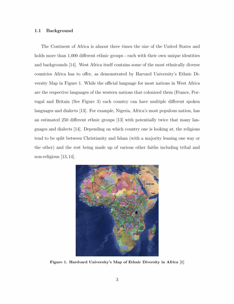
The Continent of Africa is almost three times the size of the United States and

holds more than 1,000 different ethnic groups - each with their own unique identities

and backgrounds [14]. West Africa itself contains some of the most ethnically diverse

countries Africa has to offer, as demonstrated by Harvard University’s Ethnic Di-

versity Map in Figure 1. While the official language for most nations in West Africa

are the respective languages of the western nations that colonized them (France, Por-

tugal and Britain (See Figure 3) each country can have multiple different spoken

languages and dialects [13]. For example, Nigeria, Africa’s most populous nation, has

an estimated 250 different ethnic groups [13] with potentially twice that many lan-

guages and dialects [14]. Depending on which country one is looking at, the religions

tend to be split between Christianity and Islam (with a majority leaning one way or

the other) and the rest being made up of various other faiths including tribal and

non-religious [13,14].

Figure 1. Hardvard University’s Map of Ethnic Diversity in Africa [1]

3

On top of the cultural richness that is provided by West Africa’s diversity, the re-

gion is also extremely wealthy in it’s abundance of natural resources such as diamonds,

gold, and petroleum to name just a few [13] (See Table 2 for detailed summary). How-

ever, despite the vast wealth of natural resources, mismanagement and corruption in

political systems, in addition to a series of devastating conflicts from the late 1980’s

to early 2000’s, the region (with the exception of Cabo Verde) has lacked economic

stability since gaining independence starting in the 1950’s [13,15–18]. In fact, it could

be argued that the state’s strict reliance on its natural resources has been perpetu-

ated political corruption, originally created by the colonial powers that previously

governed the West African States [15–17]. Whatever the reasons may be, it cannot

be denied that West Africa, though technically growing, holds some of the world’s

poorest nations. Eleven out of the fifteen nations (Benin, Burkina Faso, The Gambia,

Guinea, Guinea-Bissau, Liberia, Mali, Niger, Senegal, Sierra Leone, and Togo) are

currently labeled as low-income economies by The World Bank while the rest (Cabo

Verde, Cote d’Ivoire, Ghana, and Nigeria) are described and Lower-Middle-Income

economies [19].

4

Table 2. West Africa’s Natural Resources [13]

Country Natural Resources

BeninSmall offshore oil deposits, limestone,marble, timber

Burka-FassoManganese, limestone, marble, small deposits of gold, phosphates, pumics,salt

Cabo Verde Salt, Basalt rock, limestone, kaolin, fish, clay, gypsum

Cote d’IvoirePetroleum, natural gas, diamonds, manganese, iron ore, cobalt, bauxite,copper, gold, mickel, tantalum, silica sand, clay, cocoa beans, coffee, palmoil, hydropower

The Gambia Fish, clay, silica sand, titanium (rutile and ilmenite), tin, zicron

GhanaGold, timber, industrail diamonds, baxite, manganese, fish, rubber,hydropower, petroleum, silver, salt, limestone

Guinea Bauxite, iron ore, diamonds, gold, uranium, hydropower, fish, salt

Guinea-Bissaufish, timber, phosphates, bauxite, clay, granite, limestone, unexploiteddeposits of petroleum

Liberia iron ore, timber, diamonds, gold, hydropower

Mali

gold,phosphates, kaolin, salt, limestone, uranium, gypsum, granite, hydropower,note: bauxite, iron ore, manganese, tin, and copper deposits are knownbut not exploited

Nigeruranium, coal,iron ore, tin, phosphates, gold, molybdenum, gypsum, salt, petroleum

Nigerianatural gas, petroleum, tin, iron ore, coal, limestone, niobium, lead,zinc, arable land

Sengal fish, phosphates, iron ore

Sierra Leonediamonds,titanium ore, bauxite, iron ore, gold, chromite

Togophosphates,limestone, marble, arable land

The obstacles facing West African nations in their economic development and

protection of their citizens’ human rights are numerous and complicated. While

several countries in this region (mainly Nigeria and Ghana) are starting to grow

their economies, most of their development is being halted by conflicts and political

corruption within their respective nations [15]. Additionally, women in particular are

facing obstacles and injustices in their communities from Female Genital Mutilations

5

and Cuttings (FGM/C), Rape, child/forced marriages, and general restricted access

to resources and liberties [13, 20, 21]. The introduction for this thesis will examine

West Africa’s history and the factors that pushed this arguably wealthy region into

the crises that its nations find themselves in today.

1.1.1 West African History.

West Africa’s history is both complicated and fascinating. The West African

region held some of the wealthiest kingdoms of their times, was the most affected by

the Transatlantic Slave Trade, and has survived civil wars, coup d’etats, and wide-

ranging disease outbreaks that have ravaged their respective countries and made

economic and social development difficult in the following years [13,22–24].

1.1.1.1 West Africa’s Wealth.

Before the intrusion of western powers, West Africa had several major kingdoms,

all of which were extremely wealthy and heavily involved in trade with the rest of

Africa and even Europe [14, 16, 25]. For the purposes of this research, this research

team will briefly cover the first two kingdoms - the Ghana Empire and the Mali

Empire. The Ghana Empire lasted from about AD 300 - 1076 [25]. Due to the

Trans-Saharan trade and iron work, the Ghana Empire went from a village and grew

in a kingdom so large so as to warrant a political system that required the ruling of

several kings - and their respective governors - all providing loyalty and taxes to their

central government [16,25]. The wealth of the Ghana empire was its gold, something

of great value to both Northern Africa and Europe [25]. All the gold that Europeans

possessed at that time was either mined in Europe or West Africa [25]. The Ghana

empire was able to obtain their gold mines and expand its kingdom due to their skill

as iron workers, providing them the significant advantage of iron weapons against

6

their neighbors [25]. The kingdom following the Ghana Empire was the Mali Empire

which lasted from roughly 1234-1468 AD [16].

Mali’s economy was agricultural based but “supported by the profits of the flour-

ishing gold trade” [16:1-22]. The Mali Empire spread its influence to the Sudan

through the power of its “chain-mailed cavalry” [16:1-22]. The Mali Empire was then

spread west to the coastline through the militant king Sabakura, a freed slave who

seized the throne in 1285 and eventually developed the kingdom depicted in Figure

2 [16].

Figure 2. Mali Empire in 1300 AD [2]

The Mali Empire’s wealth is best illustrated in the story of its most famous king

- Mansa Munsa (1312 - 1337). Mansa Munsa gave fame to the Mali Empire on his

extravagant pilgrimage to Mecca where he was said to be accompanied by a force

of 60,000 men and 500 slaves, each of whom carried a golden rod [16].It was Mansa

Munsa’s excessive consumption and spending that earned him and his empire’s fame

throughout Northern Africa and Arabia.

The wealth and success of the Ghana and Mali empires demonstrates the wealth

and sophistication in West Africa before Europe and other Western powers became

involved. This helps to dispel the common western myth of a poor continent in need

to aid and western intervention - a myth that helped perpetuate the ideas supporting

7

colonialism.Long before the west was involved with Africa, the continent had several

kingdoms, each wealthy and governed by a relatively complex political system for its

time.

1.1.1.2 The Slave Trade and Colonialism.

Europe’s knowledge of West Africa was through the Muslim traders that trans-

ported West Africa’s gold through the Trans-Saharan routes. However, Portugal in

the early 15th century sent out sailing explorations along the western coast of Africa

in hopes of circumventing the economic middle man inorder to trade directly with

West Africa for its gold and recruit them in their fight against Islam [16]. Eventually,

Portugal would go around the African continent to India and only continue trade

with West Africa in gold, and later on, slaves [16].

Slavery was an established institution in Africa well before Europeans started

trading with West Africans [16]. However, slaves in West African society similar to a

domestic servant than a slave, who’s value was determined by the “prestige that he

awarded his master” rather than the economic value that he represented in Europe

and the Americas [16:197-199]. Though a slave never belonged to a kinship group,

he was awarded status within society [16]. However, once West Africans drained the

supply of their own slaves in trade with Europe, they started to obtain slaves through

warfare [16]. While relatively few people were sold into slavery as a yearly percent

of the population, it was mostly the young, fit and healthy - predominately men -

who were captured and sold [16]. The general historical and economic consensus that

the loss of able body labor hindered the regions of Africa affected by the slave trade

[16]. One study in the American Economic Review observed that there was a positive

correlation between areas in Africa that were most affect by the slave trade and their

ability to trust today [26]. The importance of this finding, as it relates to the West

8

African economy today, is that a willingness to trust is necessary for most economic

activities. This indicates that the slave trade is affecting West Africa’s economic

development today.

However, in the 18th century, European (specifically British) attitudes towards

the Trans-Atlantic slave trade started to change. Due to the influence of Enlight-

enment ideas and evangelical Christianity in addition with an increased interest in

“legitimate” trade and exploration, abolitionist ideas started to spread across Europe

[16:220-225]. This eventually lead to England’s criminalization of the slave trade in

1807. By 1833, the practice of slavery had been abolished throughout the entire Brit-

ish Empire [16]. England, through diplomacy, convinced several powerful European

and American nations to abolish the slave trade by 1817 [16]. However, despite naval

action taken by Britain, slavers continued to evade British ships and transport slaves

from West Africa to the Americas [16]. Due to this, there was a growing idea in Bri-

tain and Europe that the way to stop the slave trade was to go further inland and set

up legitimate trade and spread Christianity [16]. This lead to the slogan of “Chris-

tianity, Commerce, Colonization” which was the ultimate start to the colonization of

the African Continent [16:220-225].

As depicted in Figure 3, the West African region was colonized by France, England

and Portugal with the exception of Liberia; a somewhat peculiar incident of Colo-

nialism. Despite its lack of accuracy, Liberia is often considered the United States

only Colony in Africa [27]. An organization called the American Colonization Soci-

ety (ACS), founded in 1812, made up of Quakers and slave holders, wanted freeborn

Blacks and former slaves to colonize Africa [27]. The Quakers believed that freeborn

Blacks and former slaves would face better chances for freedom in Africa, while also

spreading Christianity. The slave owners, however, wanted to avoid a potential slave

uprising like the one in Haiti [27]. Despite significant disagreement from several prom-

9

inent African American figures and other white abolitionists, with the help of a few

legislators, the ACS was able to start their first colony in 1821 with 86 African Amer-

ican volunteers in modern day Liberia [27]. Upon arrival, the white ACS members

governed the colony of Liberia for several years [27]. The Americo-Liberians grew

in number over the years due to further immigration and would eventually become

pseudo colonists over the indigenous Africans there before them [17,27]. Yet, despite

several problems that the country would later on develop, Liberia would eventually

become a model for several other African Colonies wanting independence as Liberia

was one of the few free republics in Africa while colonialism in Africa was at its height

[27].

Figure 3. Africa with Colonial Powers [3]: West Africa Outlined in Black

10

France was the primary colonial power in West Africa, as evident by Figure 3.

France significantly benefited from its colonial standpoint in West Africa. In fact,

during World War I and II, France had enlisted several of its African citizens in their

armed forces to fight on the front lines in Europe [16]. The general consensus in

French colonialism was to build up the African colonies and encourage a certain level

of self-governance while still maintaining a level of Western/French superiority [16].

France’s view of colonialism was the general consensus in most of the Western world,

as evident in the famous poem “The White Man’s Burden”, written by Rudyard

Kipling in 1899:

“Take up the White Man’s burden —

Send forth the best ye breed —

Go bind your sons to exile

To serve your captives’ need;

To wait in heavy harness,

On fluttered folk and wild —

Your new-caught, sullen peoples,

Half-devil and half-child.” (1-7)

The West viewed their colonialism as a mutually beneficial arrangement - they

profited and the poor people of inferior cultures were civilized. There still exists a

debate between those in related fields concerning the extent to which colonialism af-

fects Africa today [16] However, most experts agree that colonialism did negatively

affect colonized nations. All but two countries - the former Portuguese colonies of

Guinea Biassau and Cabo Verde - gained independence in a relatively peaceful man-

ner. However, the colonial powers that colonized West African nations did little to

prepare them for Independence [17]. Additionally, some contribute colonialism to the

11

corruption of Africa’s governing bodies, which eventually lead to the region’s conflict

and economic instability [16, 17,28]

1.1.1.3 Civil Unrest.

The end of the Cold War has been “characterized by a wave of violent civil wars

that produced unprecedented humanitarian catastrophe and suffering” [17:1-9]. These

violent conflicts, starting with the first civil war in Liberia in 1991 to the coup d’etat

in Cote d’Ivoire in 2002, West Africa has been plagued with catastrophic violence

in Liberia, Sierra Leone, Mali, Niger and Cote d’Ivoire [17]. From the documented

cases of force amputations in Sierra Leon’s civil war to the cannibalistic war lords in

Liberia’s civil wars, it is not hyperbolic to claim that these wars were hell on earth

[29,30].

The reasons for these conflicts vary, though the underlining ethnic tensions and

political corruption are persistent underlining themes. The arbitrary boarders drawn

up by France, Great Britain and Portugal has magnified ethnic tensions within the

region. The arbitrary boarders continually cause social and political unrest in several

African nations [17]. Indeed, it was the arbitrary boarders drawn by France and

Great Britain concerning Gambia that caused serious problems in the secessionist

war in the Casamance region of Sengal [17]. Since these boarders were drawn with no

thought towards the existing tribes and their communal ancestry, intrastate conflicts

have spread across boarders as members of the same ancestry will often come to the

aid of their kin [17].

While ethnic tensions have and continue to influence several conflicts in West

Africa, a significant force behind these conflicts are widely attributed to general mis-

management of economic funds and political corruption [15, 18, 24]. Unlike most co-

lonial states in Asia, Africa’s road to Independence was relatively fast and surprising

12

to most of their colonial powers [17]. Additionally, all three colonial powers restric-

ted their African subjects’ ability to self-govern [17]. As a result, most African were

illiterate and lacked the necessary skills to govern a nation [17]. Furthermore, Afric-

ans became accustomed to a centralized, authoritarian form of governance from their

colonial rulers. As a result, most freed African nations placed a significant amount

of power in the hands of a few, most of whom lacked the skills necessary to succeed

[17]. As most of Africa’s wealth came from its natural resources, the mismanagement

of such resources, along with the significant debt brought on by rampant borrowing,

eventually lead to conflict within the region [13,17]. The resulting conflicts have sab-

otaged the economic growth several West African nations, spreading poverty, crime

and disease.

Figure 4. Violent Events in West Africa (1997-2012) [4]

1.1.1.4 Ebola Crisis.

The Ebola Crisis, which lasted from 2013-2016, incapacitated the countries of

Guinea, Liberia, and Sierra Leone. According to the Center for Disease Control

13

(CDC), the disease started in a small village in Guinea in December 2013 where an

18-month old boy was believed to be infected by bats [31]. Over a span of two and a

half years, the disease spread to two other nations, infecting 28,600 people and killing

11,325 [31–33]. Figure 5 provides a geographical representation of where the virus

was most effective.

Figure 5. 2016 Map of the Ebola Outbreak in West Africa [5]

Though large, the death toll is not adequately represented by those whose death

was solely caused by Ebola. Due to fear of hospitals and medical workers, created

by the rampant spread of Ebola, others who required medical attention unrelated to

Ebola failed to obtain it [22,32,33]. In addition to lives lost, these three nations had

recently experienced serious conflicts and were starting to rebuild their economies.

The loss of production, human capital, and costs associated with trade restrictions

impeded the economic and social growth of recently war-torn nations [22, 31–33].

The unbridled spread of the Ebola virus eventually lead to a global health crises that

forced the international community to intervene [31].

The rampant spread of the Ebola has several causal factors including a lack of

14

communal knowledge and training concerning disease control and prevention, insuf-

ficient reaction speed - both communally and from the international community -

and failure to recognize the importance of a “safe and dignified burial” from mul-

tiple West African communities [32:2]. However, experts place primary blame on

inadequate health services [22, 31–33]. In a report titled, “A Wake Up Call: Lessons

from Ebola for the world’s health systems”, Save the Children organization reported

that in 2012 Guinea spent an average of $9 per person on health care, compared to

a recommended minimum expenature of $86 per person [32:4]. Lack of funding was

further exacerbated by an insufficient supply of doctors, nurses and hospitals required

to contain the virus [22,31–33]. Due to the absence of necessary health care resources,

the international community was forced to get involved, costing the rest of the world

$4.3 billion [32:9].

1.1.2 Current State.

The West African region is currently home to some of the Continent’s more stable

countries (Ghana and Sengal) and also houses several countries (Ivory Coast, Liberia,

Sierra Leone) who have successfully transitioned from war to relative peace [15]. The

region, overall, has transitioned from the post Cold War conflicts to a state where

the political institutions are relatively stable. However, this transition is more or less

a transition from one type of conflict to another.

Currently, the region is under tremendous stress due to the transition from “con-

ventional and large-scale conflict events” [15:24] to instability driven by election re-

lated violence, drug trafficking, violent extremism, piracy, and overall criminality

[15].

15

1.2 Women

In West Africa, Women face significant obstacles such as early marriages, FGM/C,

a lack of education, and significantly high maternal mortality rates [13]. As you can

see from Table 3, several of West Africa’s countries lack what most developed countries

would view as basic necessities for women. The inadequate maternal care and female

education oppresses women living in these nations. Without an education and basic

maternal heath care, women will face substantially greater obstacles in their lives

compared to most men in similar economic living standards. Two of the nations in

West Africa, Niger and Seirra Leone, are leading the world in fraternity rates and

maternal mortality rates respectively [13].

16

Table 3. West African Women Statistics [13]

West AfricanCountries

Reference Countries

Metrics Binin Burkina Faso Cabo Verde Cote d’Ivoire Gambia Ghana Guinea-Bissau Guinea Liberia Mali Niger Nigeria Sengal Sierra Leone Togo South Africa USA

Mothers Mean Age at First Birth 20.3 19.4 N/A 19.8 20.9 22.6 N/A 18.9 19.2 18.8 18.1 20.3 21.5 19.2 21 N/A 26.4Maternal Mortality Ratio (dealths/100,000live births)

405 371 42 645 706 319 549 679 725 587 553 814 315 1,360 368 138 14

Infant Mortality Rate (deaths /1,000 livebirths)

52.8 72.2 21.9 55.8 60.2 35.2 85.7 50 52.2 69.5 81.1 69.8 49.1 68.4 42.2 31 5.8

Total Fertility Rate (children born perwoman)

4.77 5.71 2.24 3.38 3.52 4 4.09 4.77 5.06 6.01 6.49 5.07 4.28 4.73 4.38 2.29 1.87

Contraceptive Prevalence Rate 17.9% 25.4% N/A 15.5% 9.0% 33.0% 16.0% 8.7% 31.0% 15.6% 18.9% 13.4% 25.1% 16.6% 19.9% 54.6% 72.7%Physician Density (physician/1,000population)

0.15 0.05 0.79 0.14 0.11 0.1 0.08 0.08 0.02 0.09 0.02 0.38 0.07 0.02 0.06 0.82 2.57

Female Literacy 27.3% 29.3% 82.0% 32.5% 47.6% 71.4% 48.3% 22.8% 32.8% 22.2% 11.0% 49.7% 46.6% 37.7% 51.2% 93.4% N/AMale Literacy 49.9% 43.0% 91.7% 53.1% 63.9% 82.0% 71.8% 38.1% 62.4% 45.1% 27.3% 69.2% 69.7% 58.7% 77.3% 95.4% N/AFemale School life Expectancy 11 7 13 8 9 12 N/A 8 N/A 7 5 8 9 N/A N/A 13 16Male School Life Expectancy 14 8 13 10 9 12 N/A 10 N/A 9 6 9 9 N/A N/A 12 17

17

Figure 6 provides a geographical representation of some of the problems women

in West Africa face today. The Organization for Economic Cooperation and Devel-

opment’s (OECD’s) Development Center Published a paper by Gaelle Ferrant and

Alexandre Kolev titled “Does gender discrimination in social institutions matter for

long-term growth?”. Ferrant and Kolev’s research concluded that gender discrimina-

tion is estimated to collectively cost nations over 12 trillion USD, or roughly 16% of

2016’s global GDP [34]. Gender discrimination can be observed through forced child

marriages, FGM/C, the lack of legal standing or the loss of life and human capital

found in high maternal mortality rates [20]. For example, Despite laws providing

widows with equal legal rights as widowers towards their inheritance, accusations of

witchcraft can be used to prevent widows and daughters’ right to claim their inherit-

ance [20]. Additionally, only in Liberia and Mali do laws exist to guarantee men and

women equal access to financial services [20]. Gender discrimination actively hinders

half of any given population from contributing to the potential economic growth of a

nation. Furthermore, child marriages prevent young girls from finishing their educa-

tion by prematurely burdening them with children of their own, thereby diminishing

female labor force participation.

Figure 6. Percentage of Young Women (20-24 years) Married before the Age of 18 [6]

18

1.2.1 Conflict and Stability.

Women are both contributors and victims of conflict. For example, during the post

Cold War conflicts in West Africa systematic rape was rampant [17]. Women and

the young were often targets of such violence [17]. However, women have also been

contributors to conflict. Such examples are women being used as a recruitment tool

through rearranged marriages between members of extremist groups and young wo-

men [35]. Women and children, whether through coercion or their own convictions,

have committed suicide bombings and other acts of violent extremism [35]. Boko

Haram, earlier in its development, managed to appeal to and recruit women followers

[21]. Initially, Boko Haram educated their female members in Islam [21]. However,

such practices have diminished and women are now taught only in the house [21].

Today, Boko Haram uses women as incentives (willing or forced) for their male mem-

bers as wives, providing status and other favors [14]. As such, Boko Haram started

kidnapping girls and women, mainly in christian dominated sections of Nigeria [21].

In April, 2014, Boko Haram kidnapped over 200 schoolgirls in the town of Chibok,

causing international outrage and activist groups to join the “Bring back our girls”

campeign [21]. Nigeria’s President at the time, Goodluck Jonathan, took three weeks

before making a statement while his wife, Patience, supposedly speculated that the

girls’ abductions occurred [21]. Boko Haram continues to kidnap women and use

them as bargaining chips for recruitment and terrorist activities [21].

1.3 Department of Defense Presence in West Africa

The United State’s involvement in Africa has been relatively insignificant when

compared to other nations such as France, Portugal or Britain. However, as religious

extremism and terrorist activities increase in Africa, the United States has increased

19

their militaristic presence on the continent mainly through the United States Africa

Command (AFRICOM) [36]. Department of Defense (DoD) activity and expenditures

in West Africa have been on the rise, as seen in Figure 7. Back in 2003, President

George W. Bush sent several hundred troops to Liberia as a humanitarian peace

keeping attempt near the end of Liberia’s second civil war [37]. However, before U.S.

troops were able to reach Liberia, Nigerian troops, under the Economic Community

of West African States (ECOWAS) authority, were sent to stop the fighting and

help restore peace [30]. In more recent news, according to a npr report in 2018, the

DoD had over 1,000 personnel in the Nigeria, Niger and Mali region alone [38]. U.S.

activities in Africa go beyond that of simple expenditures and man hours. In October

of 2018, four Americans were killed during an ambush in northern Niger [38].

Figure 7. Military Expenditures in West Africa [7]

According to AFRICOM’s website, their mission is to “strengthen security forces,

counter transnational threats, and conduct crisis response in order to advance U.S.

interests and promote security, stability and safety” with local partners [39]. Ac-

cording to an article published in the Orbis Journal titled, “Assessing a Decade of

U.S. Military Strategy in Africa”, the U.S. presence in Africa, through AFRICOM,

differs from U.S. DoD presence in other continents in that AFRICOM “prioritizes

a light footprint and the priorities of African partner nations” [36:657]. AFRICOM

implements their priorities of cooperation and stability by “attempting to reduce the

20

sources of insecurity and helping to strengthen African security capabilities” [36:657].

AFRICOM’s, and by extension the U.S. Military’s, mission in Africa is to promote

stability within the continent while also promoting the U.S’s interests - particularly

against terrorist activities and extremism.

Africa’s “security, stability and safety” are primary concerns for AFRICOM [39].

Additionally, several respectable organizations, such as the UN, have declared gender

equality to be a key determinant in stability and maintaining peace [40]. Given

AFRICOM’s mission statement, researching the relationship between women and

stability could potentially determine whether DoD investment in gender equality in

Africa could assist in the promotion of AFRICOM’s mission statement.

1.4 Problem Statement

West Africa is a region with a complex history filled with various Western inter-

ventions, slavery, Colonialism and is continually dealing with ethnic, religious and

politically charged conflicts, human rights violations, and overall criminality. Several

global organizations, like the United Nations, have already started to seek out ways

to increase gender equality in West Africa and similar regions so as to encourage

stability and peace in war torn nations. However, there is little research done to

better observe and summarize the complex relationship between women and armed

conflict and the specific regions in which it may take place. Due to the absence of

quantitative research pertaining to women and conflict, this research will endeavor to

capture the relationship between conflict and women and its geographic significance,

if any exists.

21

1.5 Assumptions

As with all research, necessary and preferably valid assumptions were implemented

in order to continue with the project. Below is a comprehensive list of the assumptions

utilized in this research.

• Surveys of women in West Africa, collected over a 16 year period (1998-2014)

depicts an appropriate singular picture of women in West Africa today. In

other words, the various samples that vary over time, without any determinable

pattern, are collectively an appropriate snap shot of the region today. Provided

the format of the data set used, disparate survey samples that vary over years

and countries with no discernible pattern in location and time collection, this is

a very necessary assumption. Furthermore, after some initial analysis, utilizing

the chosen methodology, this team saw no obvious differences between women

over the collected time period, thereby validating the assumption.

• As discussed previously, the boarders separating the nations may not be the

best representation of a separation between people, culture or even national

identities. As such, the boarders separating the survey samples will be con-

sidered arbitrary. This assumption draws its argument from colonial history.

The Western nations who drew the borders were more concerned with its natural

resources than the native people’s culture and history. As such, these boarders

should be considered arbitrary when considering soci-economic factors such as

gender equality and women’s well-being.

• Niger 1998 will have to be a sufficient data sample size as it is the only survey

sample with GPS locations that were provided. This assumption is necessary

due to Demographic and Heath Survey (DHS) samples from Niger either did

22

not collect GPS data, or did, but later found them to be corrupted. Due to the

chosen methodology, this assumption does not significantly affect the analysis,

however, Niger will be under represented in the analysis due to the lack of data.

• The data has some shape in Rn and the shape of the data matters. This is

the most significant assumption behind the primary chosen methodology, To-

pological Data Analysis, and will be discussed further in the following chapters.

Researchers in Applied Topology and Data Science found this assumption to be

necessary, valid, and even additive in data analysis.

• Missing values in the data have meaning and are therefore significant to the

shape of the data. This is a common assumption in Social Science fields [41]

and provided the data set, is both necessary and valid. For example, if a

women has a NaN value for a variable describing the “Age at First Birth” for

each women. In this variable’s instance, the NaN value implies that the woman

simply has not had a child yet, implying that the NaN value protrays meaning

and therefore holds significance in the analysis. For the purposes of this paper,

this team added a binary indicator variable for NaN or missing values when

believed to indicate meaning.

• Niger, for the year 2008, had missing values for all conflict data. However, only

Nigerien women with DHS survey answers from 1998 also had accompanying

sample GPS locations. Therefore, due to the length of time between survey

sample and missing conflict data, the missing conflict event data from 2008

should not significantly affect analysis. As such, all 2008 conflict events for

Niger were made to be zero.

• The answers to the DHS survey sample questions collected, seen in Appendix

A, are a good proxy for measuring a woman’s well being. Most of the variables

23

collected were concerning a woman’s socio-economic status. Most of the liter-

ature concerning women’s well-being in relation towards stability, the women’s

socio-economic status were primary variables. As such, DHS survey questions

concerning socio-economic status was collected. However, other indicators could

be more appropriate and further research is necessary to evaluate the validate

this assumption.

• A key assumption in the analysis is that a woman’s proximity, as measured by

a 10 kilometer radius from survey sample GPS location, during a five year win-

dow of time, is an adequate measure of the stability/instability in her immediate

surroundings. While other measures of stability and/or instability could poten-

tially better capture stability, in relation to women; due to time constraints, this

assumption was used instead. Further analysis and study would be required to

validate this assumption or implement research with a better assumption.

1.6 Overview

The primary research question is concerning the relationship between treatment of

women and a region’s, nation’s, or community’s stability. This paper defines women’s

station or well-being in life through the use of the Demographic and Health Survey

(DHS) Program data and stability through conflict data gathered from The Armed

Conflict Location & Event Data Project (ACLED) database. For the purposes of

this research, “stability” is defined from a Department of Defense (DoD) view point

by observing conflict that involves the use of arms and threatens potential milit-

ary intervention. Additionally, Geospatial analysis will be implimented on important

socio-economic indicators alongside a few supervised and unsupervised machine learn-

ing algorithms. The data and the definition of conflict and stability/instability will

24

be discussed in more detail in later chapters.

The following chapter (Chapter 2) will cover an adequate overview of research

concerning women and their affect on stability. Chapter 2 will also cover the chosen

methodologies. The third chapter will give a comprehensive overview of any method-

ologies that where explored. This will leave Chapter 4 for the analysis of any findings

and chapter 5 for a conclusion of the findings and potential future work that could

be applied to this dataset or research question.

25

II. Literature Review

2.1 Overview

As discussed in the Introduction, West Africa is a large region filled with diverse

groups of peoples, cultures, communities, and histories. Provided that women are

roughly half of any given population, the theory that women and how they interact

within their communities will impact those communities. However, as it relates to

the relationship between women and stability, researchers struggle with three primary

aspects of researching this topic:

• How do is “stability” defined?

• Given the definition of stability, how do women affect stability (if at all)?

• To what extent do women affect the decided definition of stability (significant

or not)?

Provided that this research is currently being sponsored by the United States

Africa Command (AFRICOM), a military organization, this research team will be

defining stability as the lack or minimization of occurrences of armed conflict events.

Armed conflict events could be described through battles between nation states or

local militia, violent extremist attacks against unarmed civilians, or riots. The precise

definitions of stability will be revisited and more thoroughly explained in the following

chapter.

This chapter will examine previous research that attempted to examine the re-

lationship between women and stability/instability. This chapter will also provide a

general explanation concerning this research’s chosen methodology.

26

2.2 Women and Stability Research

Little quantitative research has been implemented when observing the relationship

between women and the definition of stability that this research will be focusing on.

The lack in research is in large part due to the structure/format of the data. How

does one numerically capture, in a structured manner, the intricate role women may

play in a terrorist organization, or how many women were involved in a particular

battle or riot and their socio-economic status? Despite the shortage of data, there is

plenty of qualitative research implemented on the subject.

Several prominent organizations are trying to better understand the role women

may play in terrorist organizations [42].There are reported cases of men joining terror-

ist organization in order to help pay a bride price [35]. Furthermore, in West Africa,

there are documented cases of Boko Haram forcing the kidnapped girls into arranged

marriages as a recruitment tool [35].

Research articles looking at a more direct link between women and stability, to

the extent that is normally desired in quantitative research and public policy de-

cision making, are scarce at best. However, a recent research article titled “Women’s

Participation in Peace Negotiations and the Durability of Peace”, and published in

International Interactions, found a positive correlation between the number of fe-

male signatures on peace agreements and the durability of the peace agreement [43].

Moreover, peace agreements with female signatures had a “significantly higher number

of peace agreement provisions aimed at political reform, and higher implementation

rates for provisions” [43:985]. This suggests that women may impact stability as

defined by this research team.

27

2.2.1 Women and General Stability.

While there has been little to no quantitative research applied towards women

and stability, as defined earlier, there are copious amount of research on women’s

affect towards a more general sense of stability - such as economic and/or social. The

relationship between women and stability is most researched when it comes to girls’

and women’s education and economic growth.

In economics, there has always been a positive correlation (and arguably causa-

tion) between education and economic growth [44]. In fact, education is believed to

be a leading “determinant of economic growth, employment, and earnings in mod-

ern knowledge-based economies” [44:3]. Women’s education, specifically, has been

consistently documented to have higher rates of return then men’s education [45].

Furthermore, women facing discrimination are costly to nations. According to The

Organisation for Economic Co-operation and Development (OECD), gender-based

discrimination in social institutions results in an estimated loss of USD 120 billion in

income for the West African region alone [20].

2.2.2 Hypothesis.

Given that women are roughly half of any given population, and have been doc-

umented to have significant impacts on a nation’s socio-economic stability, women

will affect the stability of a nation when it comes to armed conflict. The relationship

between women and the definition of stability, as defined in this research, will most

likely be multifaceted, complicated, and buried amongst several other cultural, his-

torical and soci-economic layers of the West African region. As such, the relationship

between women and stability, as defined in this research, is not likely to be completely

captured in a single research paper.

28

However, this research team will attempt to investigate the relationship between

women and stability through the shape of the data. It is this research teams hypothesis

that if the relationship between women and stability exist, it will be best observed

and researched by investigating the shape of the data rather than through traditional

statistical practices.

2.3 Topology

Topology, though not a established field of mathematics until the late 19th to

early 20th century, is often considered to have its origin with none other than Leon-

hard Euler [8, 46]. Euler published his paper The solution of a problem relating to

the geometry of position in 1738 with his solution to the Konigsberg bridge problem

depicted in Figure 8 below.

Figure 8. Diagram of the Konigsberg bridges [8]

The Konigsberg bridge problem, depicted in Figure 8 was as follows: is it pos-

sible to start at one point and cross Konigsberg’s seven bridges only once in a single

journey [8]. Euler solved the Konigsberg bridge problem not through strict geometric

analysis, but rather by drawing up a crude diagram of only the relevant information;

29

the bridges’ relative position to one another and the blocks of land mass [46]. Euler

proved that it was in fact impossible to make the desired journey [8]. Even though

it would be a couple hundred years after Euler published his paper that the precise

formulation of Topology as a sub-field of mathematics would be defined, Euler and

the Konigsberg bridge problem are most often attributed with the birth of Topology

[8]. The Konigsberg bridge problem is considered to be the birth of Topology be-

cause Euler took a problem concerning shape and geometry and deformed it to its

core components, ignoring irrelevant information concerning shape that often defines

Geometry’s notion of shape.

Instead of Geometry’s rigid definitions concerning shape and congruence, Topo-

logy, “deals with qualitative geometric information” [47:256]. In fact, Topology ig-

nores most quantitative information describing shape, such as distance and angle,

and instead “replaces them with the notion of infinite nearness of a point to a subset

in the underlying space.” [47:256]. Topology’s definition of shape has influenced the

spread of a joke that does a decent job of describing how Topology’s defintion of

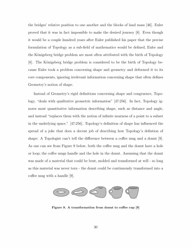
shape: A Topologist can’t tell the difference between a coffee mug and a donut [9].

As one can see from Figure 9 below, both the coffee mug and the donut have a hole

or loop; the coffee mugs handle and the hole in the donut. Assuming that the donut

was made of a material that could be bent, molded and transformed at will - so long

as this material was never torn - the donut could be continuously transformed into a

coffee mug with a handle [9].

Figure 9. A transformation from donut to coffee cup [9]

30

Though Topology has been studied for a few centuries, it has not been until recent

decades that mathematicians and data scientists have started to apply Topology’s

looser notions of shape to the world of data [46]. There are three key properties

in Topology that make the mathematics’ field potentially superior to others when

dealing with data:

• Coordinate invariance: According to this property, Topology’s study of shape

does no depend on the set of coordinates chosen [10]. according to the coordin-

ate invariance property, which is depicted in Figure 10, all three ellipses are

considered equivalent [10]. This is value added in data analysis because data

often undergoes several different transformations in the data matrix [10]. These

transformations are equivalent to simple changes in the vectors’ coordinates

[10].

Figure 10. Example of Coordinate Invariance Property [10]

• Deformation invariance: According to this property, a geometric shape can

be squashed, stretched, and deformed (provided that is is not torn) without

changing it’s topology [9]. A good example of this is humans’ natural ability

to determine equivalency between two slightly different shapes. For example,

when looking at each shape in Figure 11, a human can easily tell that each

shape is the letter “A” in different font styles [10]. The change in font style

does not change the shape or the meaning behind the shape itself; all three are

the letter “A”.

31

Figure 11. Example of Deformation Invariance Property [10]

A stricter geometric approach to this property can be seen in Figure 12. Ac-

cording to the deformation invariance property in Topology, all three shapes

are considered to be essentially the same [11]. The edges of the square can be

rounded off and the shape molded into the circle, and since the points on the

edge of the shape that were “near” each other before the deformation are still

“close” to each other after, the shapes are considered to be essentially the same

[11].

Figure 12. Geometric example of Deformation Invariance [11]

• Compressed representation: This property is one of the most useful tools when

applied to data [10].Instead of trying to describe the infinite number points and

pairwise points in the circle depicted in Figure 13, one can compress the circle

into the hexagon next to it [10]. Both capture a critical quality of the circle

(the loop) but the hexagon is infinitely easier to examine and describe [10]. This

property is beneficial when visualizing data and relationships within the data

that is currently in Rn space [10].

32

Figure 13. Compressed Representation Property Example [10]

For more information on Topology as a field of mathematics please see Munkres

[48].

2.3.1 Topological Data Analysis.

Mathematicians and data scientists recently started to apply Topology to the

world of data [46]. Topological Data Analysis (TDA) is a growing field of applied

mathematics that involves applying certain concepts and definitions derived from To-

pology to data [9]. There are two major methodologies in TDA, Persistent Homology

and MAPPER [9]. For the purposes of this research, this team will be focusing on

the MAPPER Algorithm and its applications.

2.3.1.1 MAPPER.

The MAPPER algorithm was first introduced at the Eurographics Symposium on

Point-Based Graphics by Gurjeet Singh, Facundo Memoli, and Gunnar Carlsson in

their papper Topological Methods for the Analysis of High Dimensional Data Sets and

3D object Recognition back in 2007 [49]. Since then, Singh and Carlsson and Harlan

Bennet Sexton founded the Ayasdi Company that built software that implements the

MAPPER algorithm along with providing TDA to clients. This research utilized the

Ayasdi software in its analysis and as such will use terminology created and coined

by Ayasdi.

33

The MAPPER algorithm is a statistical implementation of applying a simplicial

complex onto a topological space [49]. For more information on simplicial complexes

and how they relate to the field of Topology, please see Hatcher [50]. The MAPPER

algorithm is provided in detail by Singh et al [49:3-4], Chazal and Michel [12:7-9],

Carlsson [47:284-287], Kraft [9:12-14], and Brown et al [51:2-3]. First, define X and

Z be two separate metric spaces, and f : X −→ Z be a continuous map between

them. In application, X is the original data space in Rn, where n > 0 and has no

upper limit, Z is in R2 or R3, and f is any real function that represents an array of

data into a single point. Once in Z, an open covering U = Uii∈I will be applied. Let

f ∗(U) denote the pullback cover V in X which is obtained by cutting the connected

components in f−1(Ui) and then collecting them so as to obtain an open cover in

X space. The Mapper construction M(X,Z, f,U) is the simplicial complex that is

created by taking the nerve of the pullback cover.

M(X,Z, f,U) = N (f ∗(U)) (1)

For a more visual representation of the MAPPER algorithm described in math-

ematical terminology above, see Figure 14, provided by Fredec Chazal and Bertrand

Michel in their paper titled: “An introduction to Topological Data Analysis: funda-

mental and practical aspects for data scientists”.

34

Figure 14. MAPPER example [12]

In simpler terminology, the MAPPER algorithm creates a simplicial complex in

the original data space X by first mapping the data into another space Z through

a continuous function f , or as Ayasdi has termed it, a lens along with some define

notion of similarity (or distance) that Ayasdi as termed as a metric [52]. A lens,

in practice, can be any method that produces a single number for a point or array

in n dimensional space [52]. A metric, is just some notion of similarity or distance

between rows, such as Correlation or Euclidean distance and is often dependant on

the data format [52]. It is through this lens and metric combination that the data in

X is then mapped to Z. As such, it is the lens and metric that defines what points

in X space are “close” to each other and which are “far away”, thereby making the

lens and metric choice critical to any analysis.

Once in Z space, an “open cover” is then applied to the data. This open cover

“bins” the data points into a predetermined number of open sets that overlap by some

predetermined amount [52]. The number of open sets and the overlap between them

are parameters set by the analyst and are called the resolution and gain respectively in

the Ayasdi software [52]. Once the “neighborhoods” are defined, these neighborhoods

35

are then mapped back into the original X space where some clustering algorithm is

applied to create nodes of similar observations [52]. Nodes that share observations,

due to the overlapping of “neighborhoods”, are connected by an edges [52]. This

results in a simplicial complex that summarizes the shape of the data as defined by

a lens, a notion of similarity (or metric), the resolution and the gain.

It is within the open covers in X that some clustering algorithm will be applied,

and clusters that share points will be connected by edges and a nerve, or simplicial

complex, will be applied to the data. The number of neighborhoods that the “filtered”

data is binned into and the amount by which these neighborhoods overlap are para-

meters set by the analyst and are referred to as the resolution and gain, respectively,

in the Ayasdi software. A depiction of such a simplicial complex can be seen in Figure

15 below.

Figure 15. Mapper Simplicial Complex with Fisher’s Iris Data Set

The figure above was created in Ayasdi’s Workbench using Fisher’s Iris data set

[53], pulled from UCI’s Machine Learning Repository [54]. Fisher’s Iris data set is

made up of sepal length and width measurements of 150 flowers belonging to three

different iris flower species: setosa, versicolor, virginica. The simplicial complexes

above were created using Multidimensional Scaling (MDS) lenses, Correlation as the

metric, and a resolution of 30 with a gain of 3 (≈ 67% overlap). The percentage

overlap between the open sets is calculated by 1/(1 − gain). Figure 15 is currently

36

being colored by a density estimate of the variable sepal width; with red nodes in-

dicating the containment of rows with wide sepals and blue nodes indicating the

opposite. After some initial analysis, it can be observed that the iris flower species

setosa is all collected within the top connected component. The other two iris flower

species, versicolor and viginica, exist within the connected component at the bottom

of Figure 15. While there is some overlap, the two species - versicolor and virginica

- are decently separated within the bottom connected component. By coloring the

simplicial complexes with a petal width density estimate, one can observe that the

overlap between the two iris flower species - versicolor and virginica - occur where

petal widths are suddenly wider, and then branch off to being skinnier for either

flower species. This provides the analyst with the information that, for some reason,

the versicolor and virginica flowers that are most likely to be confused with each other

have wider petal widths then the rest of the flowers in their species. More analysis

would be necessary to know why, perhaps coloring by petal length density estimate.

2.3.1.2 Applications of MAPPER.

MAPPER, due to its unique capabilities with complex and high dimensional data

sets, has been implemented with relative success in the medical fields. In one paper,

researchers were able to identify a unique subsets of breast cancer tumors that (i)

“exhibit clear and coherent clinical characteristics” and (ii) have a 100% survival

rate [55:7265-6]. These researches were able to define these sub-groupings of cancers

patients through MAPPER by using a continuous function/lens specific to the medical

field called Disease-Specific Genomic Analysis (DSGA) [55]. They also created a Web

tool that applies their methodology - which is an implementation of MAPPER specific

to genomic data dealing with diseases [55].

Another implementation of MAPPER in the medical field is a paper published

37

in Science Translational Medicine that was able to identify three distinct subgroups

of Type 2 Diabetes (T2D) [56]. In addition to identifying three distinct sub-types

of T2D, the researchers were also able to test for specific diseases that T2D patients

are often considered high risk [56]. The study found, from it’s implementation of

the Mapper algorithm on the medical records and genotype data from 11,210 T2D

patients that each subgroup had significant correlation with defined groupings of dis-

eases that T2D is often characterized as being high risk [56]. Subtype 1 of T2D

was “characterized by T2D complications diabetic nephropathy and diabetic retino-

pathy”; Subtype 2 of T2D was “enriched for cancer malignancy and cardiovascular

diseases”; and subtype 3 of T2D was “associated most strongly with cardiovascular

diseases, neurological diseases, allergies, and HIV infections” [56:1]. They concluded

that there is a need for a more nuanced definition of T2D that might impact important

clinical decisions and doctor/patient interactions [56].

MAPPER was also implemented in fraud detection. Ayasdi analyzed highly com-

plex transaction data for one of the top 5 consumer credit card issuers - dubbed

“The Company” in Ayasdi’s report to protect client information [57]. According to

Ayasdi’s report, by looking at the shape of the data, they were able to increase the

company’s fraud detection rate from 28% to 99% for a newly identified type of fraud

[57]. Ayasdi was able to create new parameters for The Comapny’s fraud detection

algorithm. By adding the new parameters, The Company was able to maintain their

original false positive rate at 1% while also decreasing their false negative rate from

75% to 0% [57].

2.3.1.3 Topological Hierarchical Decomposition.

Topological Hierarchical Decomposition (THD) is a new application of MAPPER

that was recently developed and is currently undergoing testing and validation by

38

the Air Force Research Laboratories (AFRL) at Wright-Patterson Air Force Base

(WPAFB) in Dayton, Ohio. AFRL recently published a paper titled “HELOC Ap-

plicant Risk Performance Evaluation by Topological Hierarchical Decomposition” in

which they describe the process in detail [51:3-4]. THD is an algorithm that “decom-

poses” a dataset into smaller groupings based on an iterative application of MAPPER

[51:3]. The algorithm starts by applying MAPPER on the entire dataset X at an ini-

tial resolution N0, which is typically small (≈ 1). This starting topological model

is typically a single node with no connected components or singletons (single nodes

with very few observations that have no edges). Keeping the gain parameter g fixed

throughout the entire process, iteratively apply Mapper on X, increasing the resol-

ution by set value δN to create a topological network K. A topological network is

a topological structure, created by running MAPPER on a data set, consisting of

nodes that are connected through edges and can be seen in Figure 15. For each Ki, if

the number of data points |Xi| in this connected component is above some threshold

t > 0, a split in the original topological network has occurred. A split will result in

a branch in the THD structure starting from the current network K. If there are no

splits after applying MAPPER on a topological network, MAPPER will be imple-

mented again, increasing the resolution by δN until another split occurs [51]. This

will continue to run until there are no topological networks that meet the threshold

limit t > 0. The result will be a tree like structure with branches of different decom-

posed connected components, with the smallest connected components at the end of

the structure, which will be refereed to as leaves in this paper.

39

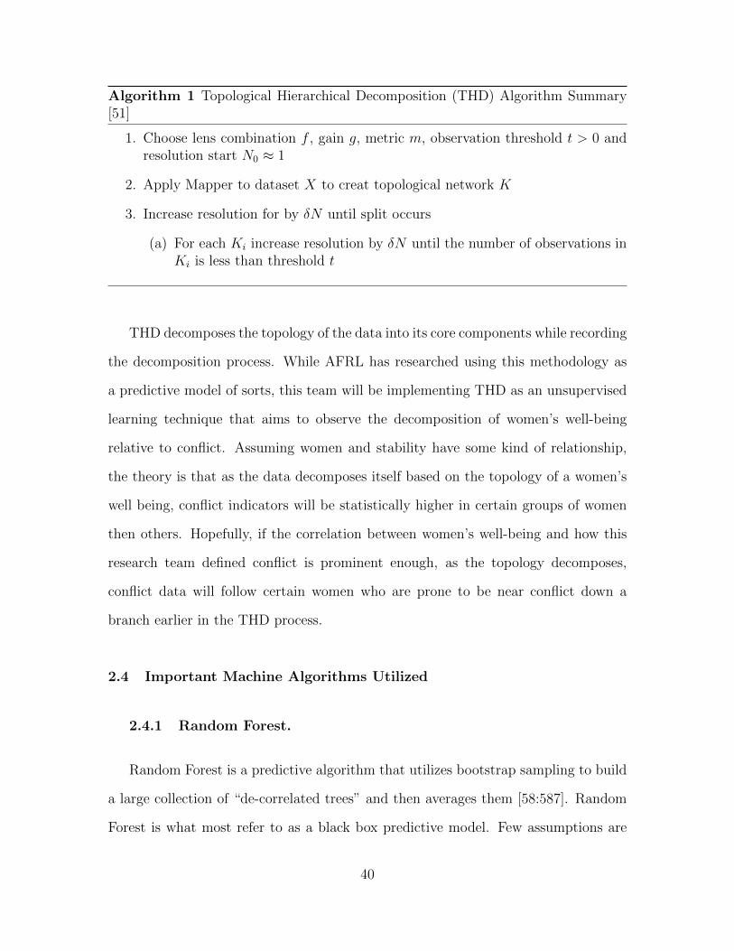
Algorithm 1 Topological Hierarchical Decomposition (THD) Algorithm Summary[51]

1. Choose lens combination f , gain g, metric m, observation threshold t > 0 andresolution start N0 ≈ 1

2. Apply Mapper to dataset X to creat topological network K

3. Increase resolution for by δN until split occurs

(a) For each Ki increase resolution by δN until the number of observations inKi is less than threshold t

THD decomposes the topology of the data into its core components while recording

the decomposition process. While AFRL has researched using this methodology as

a predictive model of sorts, this team will be implementing THD as an unsupervised

learning technique that aims to observe the decomposition of women’s well-being

relative to conflict. Assuming women and stability have some kind of relationship,

the theory is that as the data decomposes itself based on the topology of a women’s

well being, conflict indicators will be statistically higher in certain groups of women

then others. Hopefully, if the correlation between women’s well-being and how this

research team defined conflict is prominent enough, as the topology decomposes,

conflict data will follow certain women who are prone to be near conflict down a

branch earlier in the THD process.

2.4 Important Machine Algorithms Utilized

2.4.1 Random Forest.

Random Forest is a predictive algorithm that utilizes bootstrap sampling to build

a large collection of “de-correlated trees” and then averages them [58:587]. Random

Forest is what most refer to as a black box predictive model. Few assumptions are

40

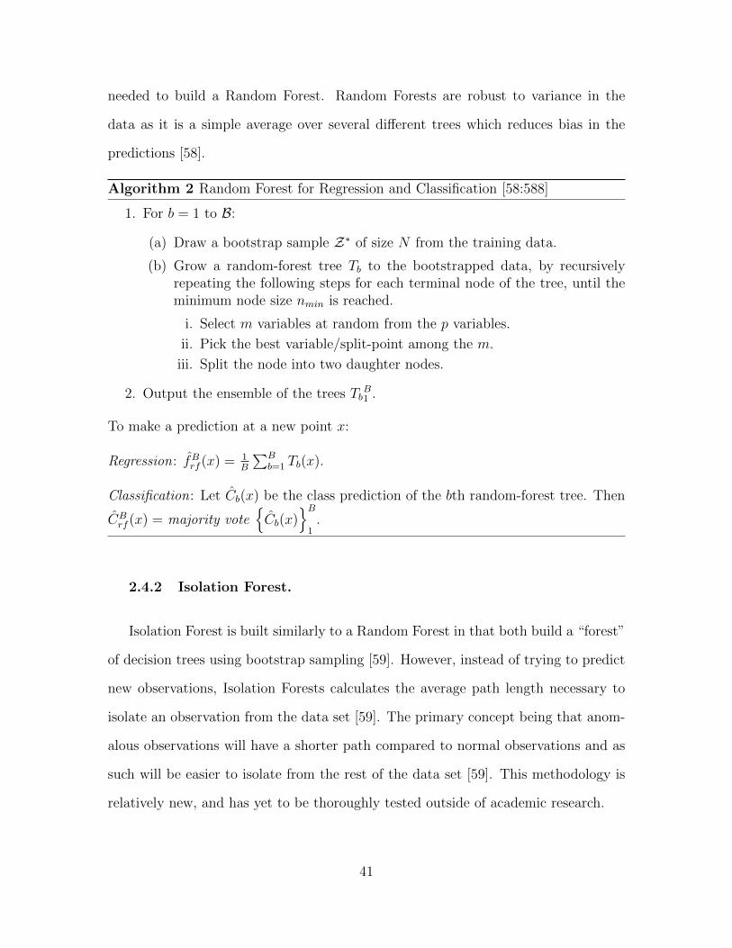
needed to build a Random Forest. Random Forests are robust to variance in the

data as it is a simple average over several different trees which reduces bias in the

predictions [58].

Algorithm 2 Random Forest for Regression and Classification [58:588]

1. For b = 1 to B:

(a) Draw a bootstrap sample Z∗ of size N from the training data.

(b) Grow a random-forest tree Tb to the bootstrapped data, by recursivelyrepeating the following steps for each terminal node of the tree, until theminimum node size nmin is reached.

i. Select m variables at random from the p variables.

ii. Pick the best variable/split-point among the m.

iii. Split the node into two daughter nodes.

2. Output the ensemble of the trees TbB1 .

To make a prediction at a new point x:

Regression: fBrf (x) = 1

B

∑Bb=1 Tb(x).

Classification: Let Cb(x) be the class prediction of the bth random-forest tree. Then

CBrf (x) = majority vote

Cb(x)

B

1.

2.4.2 Isolation Forest.

Isolation Forest is built similarly to a Random Forest in that both build a “forest”

of decision trees using bootstrap sampling [59]. However, instead of trying to predict

new observations, Isolation Forests calculates the average path length necessary to

isolate an observation from the data set [59]. The primary concept being that anom-

alous observations will have a shorter path compared to normal observations and as

such will be easier to isolate from the rest of the data set [59]. This methodology is

relatively new, and has yet to be thoroughly tested outside of academic research.

41

2.4.3 t-Distributed Stochastic Neighbor Embedding (t-SNE).

One of the lenses that was utilized for this research is a lens provided by Ay-

asdi called Neighborhood Lenses 1 and 2. Though these lenses are proprietary in

nature, according to an answer provided on Ayasdi’s Support Blog [60], the lenses

were developed from Hinton’s and Van der Maarten’s data visualization technique

t-Distributed Stochastic Neighbor Embedding (t-SNE) [61]. Therefore, even though

the precise methodology in Ayasid’s Neighborhood Lenses are proprietary, the t-SNE

algorithm is close to the one used for this paper’s models and as such will be presented

as a decent example for methodology used. The goal of all dimensionality reduction

techniques is to convert a high dimensional data set X = x1, x2, ...xn into two or

three-dimensional data set Y = y1, y2, ...yn that can be easily observed in a scatter

plot [61]. The aim of dimensionality reduction is to preserve as much of the signi-

ficant structure of the high-dimension data while mapping the data matrix X into

a lower-dimension Y [61]. Other traditional techniques, such as Principal Compon-

ent Analysis (PCA) or Multidimensional Scaling (MDS) aim to preserve some global

structure of the original data matrix X. In contrast, t-SNE aims to preserve the local

structure in the original data matrix X when mapping onto Y [61]. As such, t-SNE

is better at capturing natural clusters and groupings that could be found in the ori-

ginal high-dimension data structure X [61]. This makes t-SNE a particularly useful

as a lens in MAPPER as a defining function of “nearness” in the binning process,

described in Section 2.3.1.1 and seen in Figure 14.

The t-SNE algorithm chooses two similarity measures between pairs of points -

one for the high-dimensional structure X and one for the low-dimensional structre Y

[62]. It then attempts to create a lower-dimensional embedding that minimizes the

Kulback-Leibler (KL) divergence between the “vector of similarities between pairs

points in the original dataset and the similarities of points between pairs of points in

42

the embedding” [62:2]. The algorithm accomplishes this through non-convex optim-

ization with a randomized starting point [62]. For a closer look at the math please

see Van der Maaten’s and Hinton’s original paper [61] or a more condensed version

out of Princeton University, originally written for learning purposes [62].

2.5 Geospatial Analysis

Geospatial analysis is said to date as far back as 15,000 years ago to the Lascaux

cave in southwestern France [63]. Though crudely drawn by early man, these maps

depicts man’s earliest attempts at mapping different aspects of the world as they saw

it.

It was not until 1854, during a particularly bad cholera outbreak in London,

that geospatial analysis was seen as a valid and useful scientific method [63]. Dr.

John Snow, an English physician, decided to map out reported cholera deaths around

London while noting the locations of water pumps [63]. With this map, Dr. Snow was

able to pinpoint the location of the outbreak to a certain water pump in the city [63].

Due to his analysis, Dr. Snow was able to help halt the spread of the disease [63].

Since then, geospatial analysis has been utilized for mapping the spread of diseases,

social norms, natural disasters and even human war far [63]. Geospatial analysis was

recently utlized in the West African region during the 2013-2016 Ebola epidemic [33].

43

III. Methodology

3.1 Overview

The chosen methodology for this research project is to observe the shape of wo-

mens’ survey data in the West African region through use of Ayasdi’s Topological

Data Analysis MAPPER algorithm, Geospatial analysis, and other unsupervised and

supervised machine learning algorithms.

3.2 Topological Data Analysis (TDA) Models

All applications of MAPPER were conducted in Ayasdi’s TDA platform named

the Workbench. The lenses utilized were Neighborhood lenses 1 and 2 (see t-SNE in

Chapter 2). The only metric used was IQR Normalized Euclidean. IQR Normalized

Euclidean distance is also known as the interquartile range metric [64]. IQR Normal-

ized Euclidean normalized the distance between two columns of data based on the

interquartile range of said column [64]. See equation below:

IQR(X, Y ) =

√√√√ N∑i=1

(Xi − YiRi

)2

(2)

Where:

• X, Y = data points

• N = dimensionality of X,RN (i.e., the number of columns chosen for analysis)

• Ri is the interquartile range associated with each column i

44

3.2.1 Toplogical Hierarchical Decomposition (THD).

Two Topological Heirarchical Decompositions (THDs) were created through AFRL’s

platform tool built to interact with Ayasdi’s Workbench, both of which require Py-

thon 2.7 [65]. The first THD was built only looking at the DHS Program’s women

survey data, meaning that no variables related to conflict were included while ap-

plying MAPPER. The second THD was created using both DHS Survey Data and

the conflict matrices described further in Chapter 4. The lenses used were Neighbor-

hood lenses 1 and 2, with a gain of 1.5 (≈ 33% overlap), IQR Normalized Euclidean

metric, and a starting resolution of 1 with an iterative increase of 15. Additionally,

to establish the difference between the separate groups/connected components of in-

terest, statistical comparisons were implimented using Kolmogorov–Smirnov tests for

continuous variables and hypergeometric tests for categorical variables.

3.3 Geospatial Analysis

All maps were created using Python 3.7 [66] libraries GeoPandas [67] and GeoPlot

[68]. The shape files that located each DHS survey cite was downloaded directly from

the DHS Program website and merged with the dataset used for analysis on the

variable DHSID - see Appendix A. DHSID was the identification number that linked

each woman with her respective DHS survey cluster location.

Two additional shape datafiles were downloaded and utilized in the geospatial

analysis. The first is the World Borders shape file from thematicmapping.org [69]

so as to outline the countries being observed in the Geospatial Analysis maps. The

second is the World Cities shape file from ArcGIS Hub website [70] which were used

to show the location of large cities in any mape that was created.

The primary analysis tool utilized was spatial kernel density estimate plots using a

45

function provided in the geoplot library. According to documentation, kernel density

estimation is a unsupervised learning technique that helps to estimate the distribution

of underlining data [68]. When applied in a spatial representation, it can be used as a

way to estimate the density of points on a map and quite random noise [68]. This is a

helpful tool as it allows us to have a clearer visual understanding of where women in

certain groupings, with statistically defined qualities, are densest in their respective

regions. Provided below in Figure 16 is a map of the methodology used.

Figure 16. Methodology Map

46

IV. Analysis

4.1 Overview

This team utilized several techniques on the obtained dataset: initial statistical

analysis, Topological Data Analysis through MAPPER, Topological Hierarchical De-

composition, supervised and unsupervised machine learning algorithms and Geospa-

tial Analysis.

4.2 Data

This research team pulled data from the Integrated Public Use Microdata Series

(IPUMS) database which is part of the Institute of Social Research and Data In-

novation at the University of Minnesota and is directed by Regents Professor Steven

Ruggles [71]. The data that IPUMS housed and merged together was originally pulled

from the Demographic and Health Survey (DHS) Program [72], funded by USAID,

and from the The Armed Conflict Location & Event Data Project (ACLED) [73]. The

DHS Program collects answers to questionnaires, or “samples”, that are supposed to

be representative of the nation at large [72]. Only surveys that were conducted on

women with attached cluster longitude and latitude location information were used

for this research. A cluster, in the DHS survey context, is a randomly selected number

of households, which are “selected with Probability Proportional to Size (PPS)” for

any given selected region within a country [74]. It should be noted, however, that in

order to secure the anonymity of the survey subjects, each cluster GPS location is

provided a random dislocation buffer of a minimum of 0 kilometers to 10 kilometers,

depending on rural or urban status [72].

Using IPUMS as the sole data source had both its advantages and disadvantages.

47

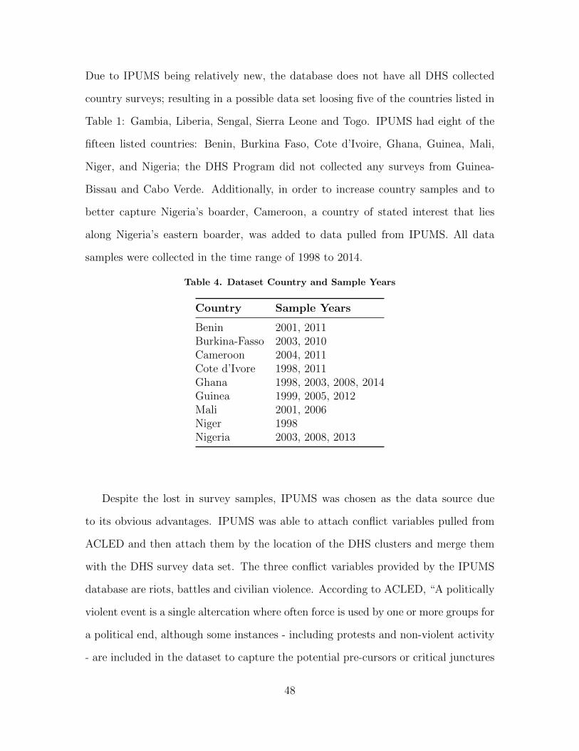
Due to IPUMS being relatively new, the database does not have all DHS collected

country surveys; resulting in a possible data set loosing five of the countries listed in

Table 1: Gambia, Liberia, Sengal, Sierra Leone and Togo. IPUMS had eight of the

fifteen listed countries: Benin, Burkina Faso, Cote d’Ivoire, Ghana, Guinea, Mali,

Niger, and Nigeria; the DHS Program did not collected any surveys from Guinea-

Bissau and Cabo Verde. Additionally, in order to increase country samples and to

better capture Nigeria’s boarder, Cameroon, a country of stated interest that lies

along Nigeria’s eastern boarder, was added to data pulled from IPUMS. All data

samples were collected in the time range of 1998 to 2014.

Table 4. Dataset Country and Sample Years

Country Sample Years

Benin 2001, 2011Burkina-Fasso 2003, 2010Cameroon 2004, 2011Cote d’Ivore 1998, 2011Ghana 1998, 2003, 2008, 2014Guinea 1999, 2005, 2012Mali 2001, 2006Niger 1998Nigeria 2003, 2008, 2013

Despite the lost in survey samples, IPUMS was chosen as the data source due

to its obvious advantages. IPUMS was able to attach conflict variables pulled from

ACLED and then attach them by the location of the DHS clusters and merge them

with the DHS survey data set. The three conflict variables provided by the IPUMS

database are riots, battles and civilian violence. According to ACLED, “A politically

violent event is a single altercation where often force is used by one or more groups for

a political end, although some instances - including protests and non-violent activity

- are included in the dataset to capture the potential pre-cursors or critical junctures

48

of a conflict” [75:7]. According the the ACLED 2017 Code book [75], the three events

used in this research are defined as such:

• Battles : A battle between two or more violent armed groups, both official

(national military) and unofficial (rebel militia).

• Riots: A violent form of demonstration

• Civilian Violence : Violence against an unarmed group of civilians at the

hands of a violent and armed group (militia, terrorist organization, or even

military).

Each of the three conflict event indicators listed above are a set of twenty variables,

ranging from 1997 to 2016, capturing the number of events that occurred within a

10 kilometer buffer around the survey cluster of each women for each given year [71].

Each set of conflict variables is a data matrix Cm×20 where C is any one of the three

conflict variable set described above, m are the number of observations in the data

set and 20 is the number of years ranging from 1998-2016 that the conflict variables

range over. The conflict variables added to the data set provided this team with a

way to view womens’ “well-being” as described by their answers to the DHS survey

and conflict around them.

Currently, the DHS Program provides their datasets in either SaS, SPSS, or

STATA data file formats. The data format in which the DHS Program provided

their data files impeded this research as this research team is unfamiliar with theses

programming languages. IPUMS, however, provided their data in CSV format which

could be loaded into a Python interface as a DataFrame using the Pandas library in

Python 3.7 [76]. This helped to decrease any uncertainty surrounding data quality

going forward.

49

Figure 17 is a map plotting the DHS sample points and is colored by country.

Figure 17 presents the spatial distribution and density of the samples gathered. For

instance, both Niger and Mali are relatively sparse in terms of samples, while Nigeria

and Ghana are both relatively dense. This disparity between number of representative

samples of women for each country is partially due to a difference in demographics.

For instance, both Nigeria and Ghana have significantly higher population densities

compared to other countries in the data sample [13]. Furthermore, each country does

not have the same number of DHS Surveys, as indicated in Table 4.

Figure 17. DHS Samples Map

4.2.1 Data Manipulation and Imputation.

4.2.1.1 Manipulation.

Due to the nature of survey data, data manipulation was required for the provided

data set. Several of the variables used, which are listed in Appendix A, were categor-

ical or nominal. According to common data manipulation practices, all nominal

and categorical variables were coded into binary indicator variables through the use

50

Python 3.7 [66] lists and dictionaries, which are provided in Appendix B. Due to

differences in country surveys, or certain questions not pertaining to all women inter-

viewed, there were several missing values in the data set. In contrast to most machine

learning assumptions, the missing values in this data set had intrinsic meaning. For

instance, a missing value in the variable pertaining to a woman’s age at their first

marriage indicates that the woman is not married. As such, instead of imputing

missing values - or other common practices in machine learning - missing values were

captured in their own binary indicator variables. In the social sciences, where missing

values often times hold meaning beyond data impurities, codeing missing values to

be binary indicator variables is considered common practice [41]. Additionally, all of

the continuous variables were normalized using the Min-Max method depicted below:

yi =xi −Min( ~X)

Max( ~X)−Min( ~X),∀i ∈ ~X (3)

Later in the data manipulation process, there was an error found in the conflict

event indicator variables. For some reason, unknown to this research team, Niger’s

riots variable for 2008 were all missing. However, since Niger only had one sample in

1998, the potential affect that the lost conflict event data could have on the analysis

is believed to be negligible at worst. As such, all the missing values for riots in Niger’s

2008 sample were simply imputed as 0 under the assumption that there were few riots

that year. Though this assumption is hardly justified, due to time constraints, it was

necessary. At the end of the data manipulation process, the data set was left with

255, 221 Observations.

51

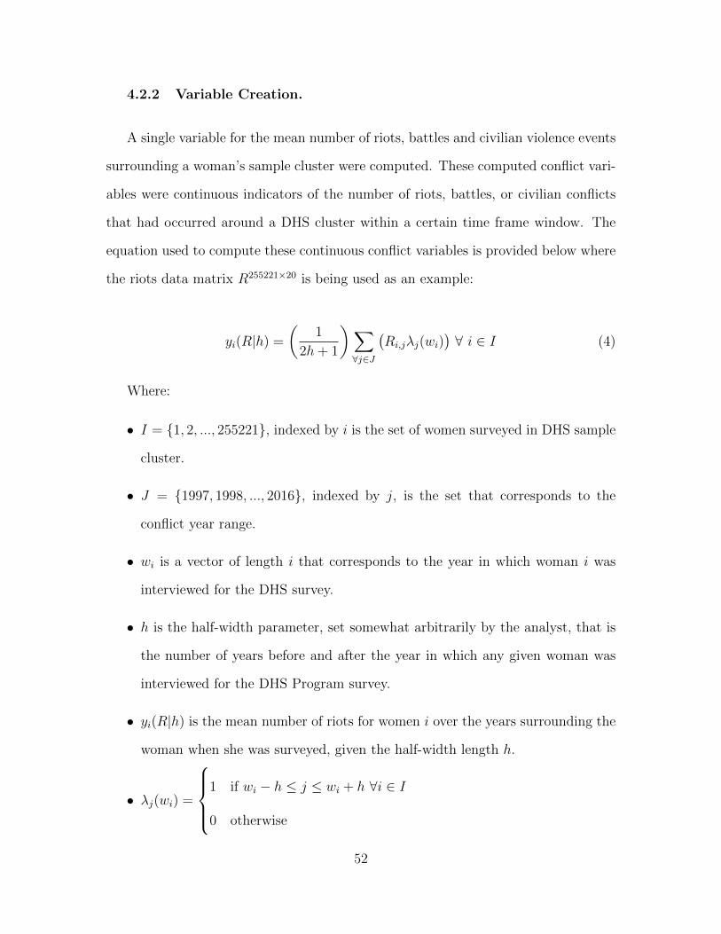
4.2.2 Variable Creation.

A single variable for the mean number of riots, battles and civilian violence events

surrounding a woman’s sample cluster were computed. These computed conflict vari-

ables were continuous indicators of the number of riots, battles, or civilian conflicts

that had occurred around a DHS cluster within a certain time frame window. The

equation used to compute these continuous conflict variables is provided below where

the riots data matrix R255221×20 is being used as an example:

yi(R|h) =

(1

2h+ 1

)∑∀j∈J

(Ri,jλj(wi)

)∀ i ∈ I (4)

Where:

• I = 1, 2, ..., 255221, indexed by i is the set of women surveyed in DHS sample

cluster.

• J = 1997, 1998, ..., 2016, indexed by j, is the set that corresponds to the

conflict year range.

• wi is a vector of length i that corresponds to the year in which woman i was

interviewed for the DHS survey.

• h is the half-width parameter, set somewhat arbitrarily by the analyst, that is

the number of years before and after the year in which any given woman was

interviewed for the DHS Program survey.

• yi(R|h) is the mean number of riots for women i over the years surrounding the

woman when she was surveyed, given the half-width length h.

• λj(wi) =

1 if wi − h ≤ j ≤ wi + h ∀i ∈ I

0 otherwise

52

For this research, h = 2 years. This h value means that for each woman in

the data set, there is a pseudo-confidence interval of length 5 around each woman’s

correlated conflict events - 2 years before and 2 years after plus the year in which

she was interviewed. The reasoning behind setting the length of this interval to 5

years was that if there is some kind of correlation behind a woman’s well-being and

stability/conflict, that a 5 year window would be a sufficient time length to capture

the conditions of each woman’s surrounding. Again, this is a parameter set by the

analyst and can be changed and further tested in later research.

Figure 18 below are box plots of the continuous variables created with h = 2.

As one can observe, the mean for each of these variables (Figure 18a = yi(R|h),

Figure 18b = yi(B|h), and Figure 18c = yi(C|h)) are close to zero. However, each

mean conflict variable has a significant number of extreme outliers with some women

experiencing an average of over 140 riots per year near them within a five year period.

53

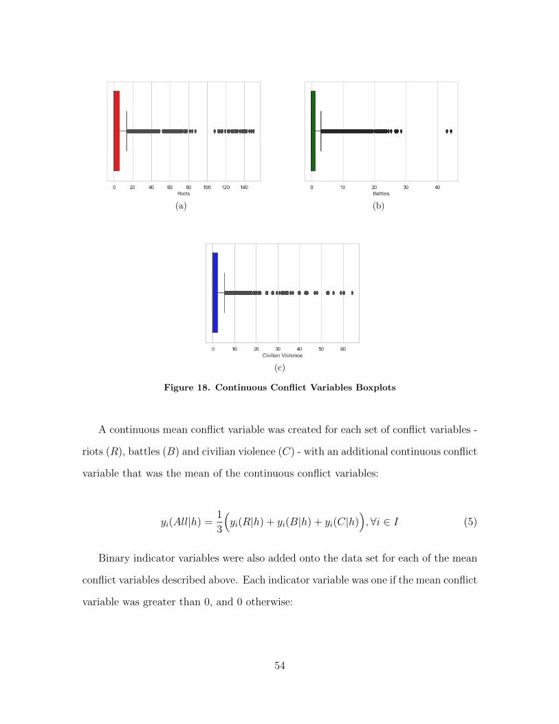
(a) (b)

(c)

Figure 18. Continuous Conflict Variables Boxplots

A continuous mean conflict variable was created for each set of conflict variables -

riots (R), battles (B) and civilian violence (C) - with an additional continuous conflict

variable that was the mean of the continuous conflict variables:

yi(All|h) =1

3

(yi(R|h) + yi(B|h) + yi(C|h)

),∀i ∈ I (5)

Binary indicator variables were also added onto the data set for each of the mean

conflict variables described above. Each indicator variable was one if the mean conflict

variable was greater than 0, and 0 otherwise:

54

bi(R|h) =

1 if yi(R|h) > 0

0 Otherwise

(6)

The conflict binary indicator variables, depicted above for riots, was utilized for

Analysis purposes while examining TDA models.

4.2.3 Machine Learning Variable Creation.

Three different sets of conflict variables were created using the random forest and

isolation forest algorithms.

4.2.3.1 Regression Random Forest Predictions.

A Regression Random Forest algorithm was trained to predict the number of

mean conflict events for each conflict type (yi(R|h), yi(B|h), yi(C|h), yi(All|h)) using

the Sklearn Python library [77]. The algorithm was trained on 75% of a randomly

selected subset of the data set, and then tested on the remaining 25% of the data

set. The predictor variables used to predict the Random Forest models were only

variables that represented a woman’s well-being; i.e. answers to the DHS Program’s

survey questions. Table 5 below is the Mean Squared Error (MSE) and adjusted R2

for each trained model when applied to the testing dataset.

Table 5. Regression Random Forest Model Scores

Dependant Variable MSE R2adj

yi(R|h) 151.947 0.173yi(B|h) 5.961 0.167yi(C|h) 11.206 0.176yi(All|h) 250.247 0.207

55

The women’s survey data, by itself, were not good predictors of conflict. The

highest R2adj value was 0.207 with a Mean squared error (MSE) equal to 250.247 con-

flict events. However, though slight at best, the predictive values for the continuous

conflict variables - which will be defined as yi(R|h)∧

, yi(B|h)∧

, yi(C|h)∧

, and yi(All|h)∧

-

are useful when trying to see how women and conflict interact in TDA models built

using MAPPER.

In addition to the four predicted continuous conflict variables, the absolute differ-

ence between the true conflict events and the predicted conflict events were calculated

for each woman. See equation 7 for reference:

riotsabsi = |yi(R|h)− yi(R|h)∧

|,∀i ∈ I (7)

The absolute difference between the ground truth and predicted values will be

useful when observing which observations were harder to predict than others and

where they exist in the topology of the data. Additional statistical tests can be

administered to determine any particular traits between hard to predict observations

and others within the Ayasdi workbench.

4.2.3.2 Isolation Forest Anomaly Scores.

As mentioned in the previous chapter, isolation forests are used to find anomalous

observations. Using the Sklearn Python library [77], two different isolation forests,

utilizing bootstrap sampling, were built. One was built on a subset containing only the

DHS Program woman survey answers, X i×363women where i is the number of observations

in the data set (255,221). The other isolation forest was built using the augmented

matrix of the DHS Program women survey answers and all three separate conflict

56

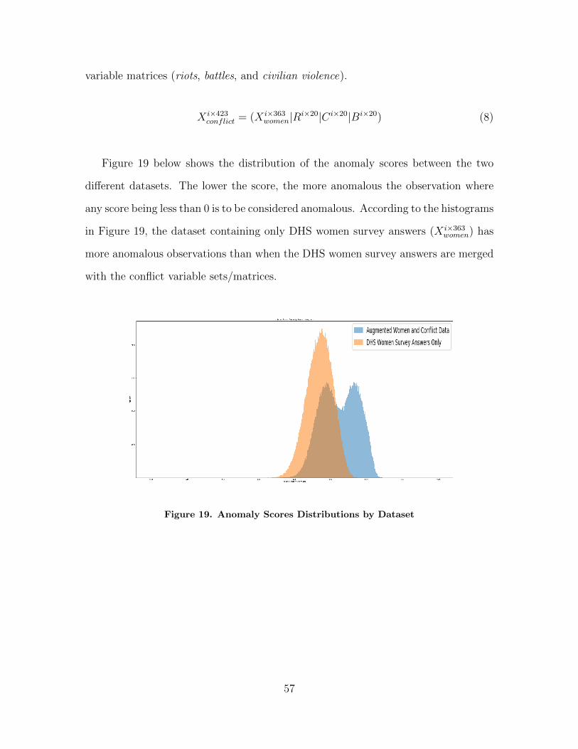
variable matrices (riots, battles, and civilian violence).

X i×423conflict = (X i×363

women|Ri×20|Ci×20|Bi×20) (8)

Figure 19 below shows the distribution of the anomaly scores between the two

different datasets. The lower the score, the more anomalous the observation where

any score being less than 0 is to be considered anomalous. According to the histograms

in Figure 19, the dataset containing only DHS women survey answers (X i×363women) has

more anomalous observations than when the DHS women survey answers are merged

with the conflict variable sets/matrices.

Figure 19. Anomaly Scores Distributions by Dataset

57

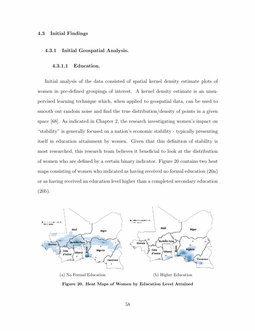
4.3 Initial Findings

4.3.1 Initial Geospatial Analysis.

4.3.1.1 Education.

Initial analysis of the data consisted of spatial kernel density estimate plots of

women in pre-defined groupings of interest. A kernel density estimate is an unsu-

pervised learning technique which, when applied to geospatial data, can be used to

smooth out random noise and find the true distribution/density of points in a given

space [68]. As indicated in Chapter 2, the research investigating women’s impact on

“stability” is generally focused on a nation’s economic stability - typically presenting

itself in education attainment by women. Given that this definition of stability is

most researched, this research team believes it beneficial to look at the distribution

of women who are defined by a certain binary indicator. Figure 20 contains two heat

maps consisting of women who indicated as having received no formal education (20a)

or as having received an education level higher than a completed secondary education

(20b).

(a) No Formal Education (b) Higher Education

Figure 20. Heat Maps of Women by Education Level Attained

58

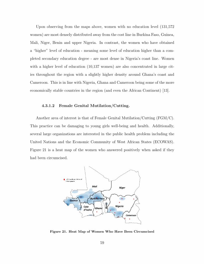
Upon observing from the maps above, women with no education level (131,572

women) are most densely distributed away from the cost line in Burkina Faso, Guinea,

Mali, Niger, Benin and upper Nigeria. In contrast, the women who have obtained

a “higher” level of education - meaning some level of education higher than a com-

pleted secondary education degree - are most dense in Nigeria’s coast line. Women

with a higher level of education (10,137 women) are also concentrated in large cit-

ies throughout the region with a slightly higher density around Ghana’s coast and

Cameroon. This is in line with Nigeria, Ghana and Cameroon being some of the more

economically stable countries in the region (and even the African Continent) [13].

4.3.1.2 Female Genital Mutilation/Cutting.

Another area of interest is that of Female Genital Mutilation/Cutting (FGM/C).

This practice can be damaging to young girls well-being and health. Additionally,

several large organizations are interested in the public health problem including the

United Nations and the Economic Community of West African States (ECOWAS).

Figure 21 is a heat map of the women who answered positively when asked if they

had been circumcised.

Figure 21. Heat Map of Women Who Have Been Circumcised

59

In Figure 21, the concentration of FGM/C is in Mali, Burkina Faso, Guinea and

Coastal Nigeria.

4.3.1.3 Anomalous Women.

An additional research question of interest was observing women who would be

considered as “anomalous” through the isolation forest algorithm, their spatial density

estimate maps, and what dimensions in the data set might account for their “anomal-

ous” classification. Figure 22 below is the heat map showing the density distribution

of the 7,786 women who had anomaly scores less than 0 (which according to Sklean’s

isolation forest documentation would be considered strictly anomalous) [77].

Figure 22. Heat Map of Women with Anomaly Scores < 0

Statistical comparisons in Ayasdi Workbench indicated that the anomalous women

not only experienced more instances of violence then the rest of the dataset, but

also had higher values associated with the mean number of conflict events described

Section 4.2.2 above. Additionally, the anomalous women were better educated overall,

60

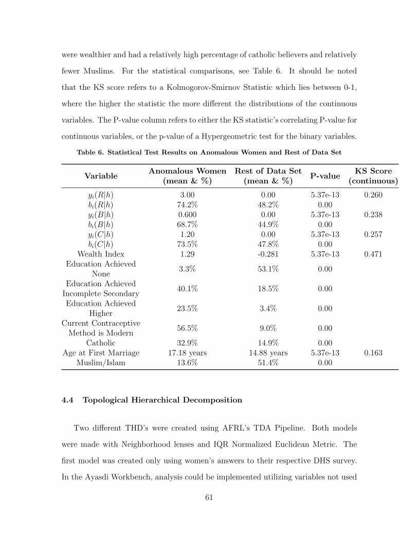
were wealthier and had a relatively high percentage of catholic believers and relatively

fewer Muslims. For the statistical comparisons, see Table 6. It should be noted

that the KS score refers to a Kolmogorov-Smirnov Statistic which lies between 0-1,

where the higher the statistic the more different the distributions of the continuous

variables. The P-value column refers to either the KS statistic’s correlating P-value for

continuous variables, or the p-value of a Hypergeometric test for the binary variables.

Table 6. Statistical Test Results on Anomalous Women and Rest of Data Set

VariableAnomalous Women

(mean & %)Rest of Data Set

(mean & %)P-value

KS Score(continuous)

yi(R|h) 3.00 0.00 5.37e-13 0.260bi(R|h) 74.2% 48.2% 0.00yi(B|h) 0.600 0.00 5.37e-13 0.238bi(B|h) 68.7% 44.9% 0.00yi(C|h) 1.20 0.00 5.37e-13 0.257bi(C|h) 73.5% 47.8% 0.00

Wealth Index 1.29 -0.281 5.37e-13 0.471Education Achieved

None3.3% 53.1% 0.00

Education AchievedIncomplete Secondary

40.1% 18.5% 0.00

Education AchievedHigher

23.5% 3.4% 0.00

Current ContraceptiveMethod is Modern

56.5% 9.0% 0.00

Catholic 32.9% 14.9% 0.00Age at First Marriage 17.18 years 14.88 years 5.37e-13 0.163

Muslim/Islam 13.6% 51.4% 0.00

4.4 Topological Hierarchical Decomposition

Two different THD’s were created using AFRL’s TDA Pipeline. Both models

were made with Neighborhood lenses and IQR Normalized Euclidean Metric. The

first model was created only using women’s answers to their respective DHS survey.

In the Ayasdi Workbench, analysis could be implemented utilizing variables not used

61

to build the model. Therefore, even though no conflict variables were used to build

the first THD model, the research team was able to track conflict variables throughout

the topology’s decomposition. The second THD model was created using the DHS

survey data augmented with the conflict data (see Equation 8).

4.4.1 DHS Data.

Figure 23 is a summary of the of the THD model created using only DHS survey

data. The blocks represent connected components that broke off from the main data

structure and the number in circles are naming the different splits for reference.

Figure 23. Summary of THD Model with Only DHS Data

The data is first split into two primary groups (and therefore most prominent

dimensions) of women, with 1.0 being married women and 1.1 being single women

with no children. The connected component made up of only single women with no

children was further split into three primary groups. The first group (3.0) contains

women who are poorer, uneducated and currently working with a mean age of 19.

The next two groups (3.1 and 3.2) consists of what seems to be mainly full-time

students (primarily college) and seem to be divided mainly by geographic location;

62

3.1 is mainly Nigerian while 3.2 has mainly Ghanaian and Cameroonian women. Each

grouping then splits further based mainly on variables describing FGM/C.

Split 2 in Figure 23 splits married women into women with children and women

without children. Following married women with children (which was a majority of

the dataset), this connected component is split further at split 4 into five separate

connected components. These connected components differ mainly in the number of

children over a 5 year period who have died and the age at which they died. These

women are then split further based on Education levels, wealth, Urban status, and

FGM/C.

Throughout the decomposition of the data set there was no single branch or con-

nected component with an obvious concentration of conflict events. However, at the

very end of the decomposition, two connected components had slightly higher concen-

tration of conflict events (as a proportion) compared to others (8.0 and 8.1). After

applying statistical test on both of these groups, both groups had higher levels of

education attainments, higher wealth indices, lower number of women who had been

circumcised, greater access to birth control, and higher mean ages at first marriage

and first birth. Essentially, most western women would want to be in these connec-

ted components, however, each had higher instances of conflict events and therefore

instability. Figure 24 below depicts the spatial density maps for the women in the

different connected components.

63

(a) 8.0 (b) 8.1

Figure 24. Spatial Density Maps of Women in THD1 Connected Components

4.4.2 DHS and ACLED Data.

The second THD model created used the data set made up of the DHS survey

data merged with the conflict events data matrices (see Equation 8). With the added

60 dimensions in the data matrix the shape/topology of the data was affected. As

such, the women in the second THD model decomposed differently compared to the

first THD model. Figure 25 is the summary of the DHS Survey and ACLED data

THD model that was created using Neighborhood lenses, IQR Normalized Euclidean

metric and a gain of 1.5 (≈ 33% overlap).

64

Figure 25. Summary of THD Model with DHS and ACLED Data

The first split at 1 was separating connected components that held extreme mean

conflict variable values. Additionally, it seems that it split these extreme components

(1.1 - 1.6) into specific time and spatially spread out events. The second split (labeled

2 in Figure 25) splits the women in a similar manner to the first THD model - married

women in 2.0 and single women in 2.2 - except that this split created a third connected

component (2.1). In this connected component (2.1) 99% of the remaining conflict

events ended up residing in connected component 2.1 (96,459 women). The splits in

the branch started by 2.1 seem to be broken up mainly by specific conflict events,

driven by the conflict matrices (see equation 8). The heat map that represents the

spatial location and density of these women in connected component 2.1 can be

observed in Figure 26 below.

65

Figure 26. Heat Map for Women in 2.1 Node of THD model with DHS and ALCEDData

Figure 26 displays women, in connected component 2.1, that appear to be centered

around larger more densely populated areas. The women in this connected component

tended to be wealthier, younger and better educated.

Furthermore, when observing the other two connected components (2.0 and 2.2)

that were brought out from connected component 1.0 (see Figure 25), one can observe

that each connected component contains women who are slightly poorer and live in

rural areas. Figure 27 shows each connected component, connected component 2.0

being Figure 27a and connected component 2.2 being Figure 27b.

(a) 2.0 (b) 2.2

Figure 27. Heat Maps of Women in Connected Components Lower Conflict Events

66

As one can observe from both Figure 27a and 27b, especially when compared to

Figure 26, the women in connected components 2.0 and 2.2 are considerably more

spread out compared to connected component 2.1, which contains 99.9% of the re-

maining violence. The women in connected component 2.1 appear to be more con-

centrated around cities.

67

V. Conclusions and Future Research

5.1 Discussion

After implementing a Topological Hierarchical Decomposition on two slightly dif-

ferent sets of data, each a representative random sample of women from their respect-

ive country, it would appear that there is no significant correlation between women

and stability as defined in this paper. The first THD decomposed the women based

solely on their answers to the DHS survey while disregarding time, location or con-

flict data. Ideally, if there is a correlation between women and stability, or rather

instability, women who had seen higher instances of conflict events would gather to-

gether. While this did occur in select connected components of different branches,

there did not seem to be an obvious reason driving the decomposition with respect

to conflict. The nodes with slightly higher instances of violence seemed to contain

women that, according to western standards, are more fortunate compared to other

women in the data sample. Upon closer examination, most of these women resided

in urban areas and were concentrated around larger cities. From these findings, there

are two plausible conclusions.

One plausible conclusion is that conflict, in developing or under developed nations,

is correlated with women who are more economically and socially secure. It could be

hypothesised that as people are less encumbered by the simple desire to survive day

to day and are provided more free or leisure time due to technological and economic

advances spend more time and resources on education and other self-development

activities. However, as education and leisure time rises, especially in a region where

lingering effects of colonialism exists and extremist views are rampant, discontent

and the ability to communicate and desire change also increases. It is possible that

as a nation develops in a politically unstable environment that there is a inverse

68

relationship between economic and social stability and conflict events. As people are

provided with the ability to voice their discontent through violent actions - in that

their not just living day to day - people will do so until a more politically stable

environment is created. This “conclusion”, however, is simply a hypothesis and far

from being substantiated solely on this research. Further investigation would be

necessary to substantiate this hypothesis.

However, it is true that these women appeared to be concentrated around cities

and urban areas and that cities, on average, have more economic opportunities, edu-

cational institutions, and jobs requiring higher levels of educations. Cities are also

where conflict events tend to occur. The second plausible conclusion, and what is

arguably the more likely conclusion, is that women have no direct correlation with

conflict and any correlation that was observed had more to do with the their location

then the woman’s well-being. The probability of observing women with more eco-

nomic and social freedom tend to be higher in urban areas. Perhaps the correlation

that can by hypothesised between a woman’s well-being and instability argued before

is happenstance and is rather proximity to a more populous area. Both conclusions,

however, would need to be investigated further.

5.2 Future Research

The primary utility that this paper provided was the structuring of a way to

observe the relationship between women and stability. Most research trying to cap-

ture this relationship has defined stability through economic terminology: economic

growth, Gross Domestic Product (GDP), GPD per capita, and so on. However, from

a DoD perspective, little to no research has been implemented when defining sta-

bility through conflict that may require military intervention. A significant reason

69

for this is data quality, structure and availability. However, even as data becomes

more available, the complexity of the data creates problems when trying to apply

a methodology. Topological Data Analysis, particularly MAPPER, can handle data

with high complexity better then traditional methods. Furthermore, the primary as-

sumption driving the MAPPER algorithm is that the shape of the data should drive

the analysis of the data; an assumption that analysts implicitly execute anyways.

By utilizing a TDA methodology, analysts can look at women in relation to conflict

in such a way that traditional statistical analysis would never permit provided the

complexity of the current available data.

As the IPUMS database grows to include more countries, the methodology applied

in this research will become easier and faster to apply. While the data cleaning process

implemented in this paper was long and exhaustive, through writing several variable

specific dictionaries and lists, this process could potentially be automated. A Python

GUI could be built to make the data pulling and cleaning process more user friendly.

Furthermore, depending on the coding and database management abilities of the

team, the methods utilized by this research team could be drastically expanded.

Due to time constraints, that this team only looked at specific economic and social

indicators of women’s well being. Though it would cut down on sample size and also

increase time spent on data cleaning, the DHS Program also collects biomarker in-

formation such as weight, height and even blood samples. DHS Program also collects

survey information from men and children. The data sample could be expanded by

adding these new dimensions and drastically different results could be observed. Fur-

thermore, this research team looked at the relationship between women and conflict

through a women’s proximity to conflict as defined through the IPUMS database.

However, this definition could be expanded. Other teams could bypass the IPUMS

database and combine the ACLED, DHS and any other database that have geospatial

70

locations differently. Other teams could try to define “proximity” to conflict more

strictly instead of this teams forced definition due to time and data availability con-

straints. Also, this team did not control for population density differences, which,

later on, proved to be potentially detrimental to the analysis. If this team had con-

trolled for population density differences in the conflict indicators, such as conflict

events per capita, perhaps the topology of the data would have decomposed differ-

ently. For future studies, a control for population densities in conflict event numbers

should be first to be implemented.

Furthermore, this team only observed the data collected through one lens and met-

ric combination - Neighborhood lenses and IQR Normalized Euclidean metric. Other

lens and metric combinations could define “nearness” of observations completely dif-

ferently compared to this paper’s chosen combination, which could potentially better

capture the relationship between women and stability. A more thorough comparison

and validation of lens and metric combinations would be needed to either confirm or

deny this paper’s conclusions.

71

Appendix A. Variables

Name Description

DHSID Key to link DHS clusters to context data (string)

COUNTRY Country

INTYEAR Year of interview

WEALTHS Wealth index factor score (5 decimals)

RELIGION Religion

PREGTERMINEver had pregnancy terminate via abortion,

miscarriage or stillbirth

FLOOR Main material of floor

COOKFUEL Type of fuel household uses for cooking

TOILETTYPE Type of toilet facility

DRINKWTR Major source of drinking water

WKCURRJOB Woman’s occupation

WKEMPLOYWHENRespondent works all year, seasonally, or

occasionally

WKEARNTYPE Type of earnings for respondent’s work

HUSJOB Partner’s Occupation

LITBRIG Literacy bridging variable

EDACHIEVER Summary educational achievement

HUSEDACHIEVER Husband’s summary educational achievement)

NEWSBRIG Reads newspaper: Bridging variable

RADIOBRIG Listens to radio: Bridging variable

TVBRIG Watches television: Bridging variable

DECBIGHH Final say on making large household purchases

DECFEMEARN Final say on spending woman’s earnings

72

FERTPREF Fertility preferences

UNMETNEED2 Unmet need for Family Planning (2nd def)

IDEALGIRLS Ideal number of boy children

IDEALBOYS Ideal number of girl children

HUSFERTPREF Husband’s desire for children

FPKNOTYP Know any type of family planning method

FPMETHNOW Current method of family planning

FPRADIOHR Heard family planning message on radio

FPPOSTHR Seen family planning message on poster or pamphlet

FPLASTSRCS Last source for family planning ofr current users, standard-

ized

AIDSHEARD Heard of AIDS

STIHEARD Heard of AIDS or other sexually transmitted infections

FCINTENDDAU Intends to have daughter(s) circumcised in future

FCCONTINU FGM/C should continue or stop

FCINFIB Vaginal area sewn closed for FGM/C

FCNICK Genital area nicked without removing flesh

FCFLESH Flesh removed from genital area for own FGM/C

FCCIRC Ever circumcised

UNION1MORE Woman had one or more than one union

DURMARGRP Marital or cohabitation duration (grouped)

MARSTAT Woman’s current marital or union status

URBAN Urban-rural status

HUSBINHOME Husban/partner lives in woman’s household

AGE Age

HHMEMTOTAL Total number of household members

73

HHELIGWOMEN Number of eligible women in household

HHKIDLT5 number of children under 5 in household

AGEFRSTMAR Age at first marriage

CHEB Total children ever born

SONSATHOME Number of own sons living at home

DAUSATHOME Number of own daughters living at home

SONSAWAYHOME Number of own sons living away from home

DAUSAWAYHOME Number of own Daughters living away from home

SONDIED Numbr of own sons who have died

DAUDIED Number of own daughters who have died

CHEBALIVE Total number of living children born to respondent

AGEAT1STBIRTH Age at first birth

HHEADAGE Age of household head

KIDAGEDIEDIMP Child’s age at death in months (including imputed) - up to

20

DELDOC Doctor gave delivery care (in last 5 years for up to 6 chil-

dren)

DELTBATraditional birth attendant gave deliery care (in last 5 years

for up to 6 children)

DELOTH Other person gave delivery care (in last 5 years for up to 6

children)

DELNONE No one gave delivery care (in last 5 years for up to 6 children)

DELCESR Delivery by caesarian section (in last 5 years for up to 6

children)

ANCARE Received prenatal care (in last 5 years for up to 6 children)

74

ANCAREDOC Doctor gave prenatal care (in last 5 years for up to 6 chil-

dren)

RIOTS Riots annual time-series (20 variables: 1997 - 2016)

BATTLES Battles annual time-series (20 variables: 1997-2016)

CIVILIAN VIOLENCE Violencce against civilians annual time-series (20 variables:

1997-2016)

75

Appendix B. Variable Dictionaries and Lists

The following code describes the dictionaries and lists utilized to manipulate the

data used for the Topological Data Analysis.

The following Python packages were used:

• numpy >= 1.15.2 [78]

# −∗− coding: utf−8 −∗−

”””

Created on Thu Oct 11 15:10:46 2018

@author: Michaela

”””

import numpy as np

#Dict for country code and country name

country dict =

120: ’Cameroon’,

148: ’Chad’,

204: ’Benin’,

288: ’Ghana’,

324: ’Guinea’,

384: ’Ivory Coast’,

466: ’Mali’,

562: ’Niger’ ,

76

566: ’Nigeria’ ,

686: ’Sengal’ ,

854: ’Burkina Faso’

#indicator variable for if husband is in home or not

husbinhome dict =

0: ’husband home’,

1: ’hus&wif live apart’ ,

9: ’not married’

#indicator variables for woman’s declared religion

religion dict =

100: ’Muslim/Islam’,

200: ’Christian’ ,

210: ’Catholic’ ,

220: ’Protestant’ ,

221: ’Anglican’,

222: ’Methodist’,

223: ’Presbyterian’ ,

224: ’Lutheran’,

225: ’Baptist’ ,

226: ’Salvation Army’,

230: ’Pentacostal/Charismatic/Evangelical’,

231: ’Apostolic Sect’ ,

232: ’Seventh Day Adventist/Baptist’,

233: ’Jehovah Witnesses’,

77

234: ’Universal’ ,

240: ’Other Chirstian, unspecified/general’ ,

241: ’Other Protestant, unspecified ’ ,

250: ’Other Chirstianm specified’ ,

251: ’Ethiopian Orthodox’,

252: ’ Celestial Church of Christ’,

253: ’African Zionist ’ ,

254: ’Munu Mwama (African Pentocostal)’,

255: ’United Faith Church’,

256: ’African Orthodox Church’,

257: ’Evangelical Luteran Church in Namibia’,

258: ’Lesotho Evangelical Church’,

259: ’Kimbanguist’,

260: ’Orthadox’,

261: ’Mammon’,

300: ’Other, not Christian or Islam’ ,

301: ’Hindu’,

302: ’Sikh’ ,

303: ’Buddhist/Neo−Buddhist’,

305: ’Jewish’,

306: ’Parsi/Zoroastrian’ ,

307: ’Doni−Polo’,

308: ’Sanamahi’,

309: ’Bahai’,

310: ’Bisaka group/Faith of Unity’,

311: ’Kirat’ ,

78

400: ’Traditional/Spritual/Animist’,

401: ’Traditional ’ ,

402: ’ Spiritual ’ ,

403: ’Animist’,

404: ’Voodoo’,

500: ’No Religion’,

600: ’Other’,

601: ’Religion 1’ ,



604: ’Religion 4’

#Dict for if a woman had more than 1 union

union1more dict =

1: ’union1more yes’, #if its zero is also no

8: ’union1more missing’,

9: ’union1more niu’

#Dict for indicator variable for woman’s marital status

currmarr dict = #currently married dictionary

0: ’never married’,

1: ’currently married’ ,

2: ’previously married’ ,

8: ’currmarr missing’

79

#Dict for highest education acheived by woman

edachiever dict =

0: ’no education’,

1: ’incomplete primary’,

2: ’complete primary’,

3: ’incomplete secondary’,

4: ’complete secondary’,

5: ’higher’ ,

8: ’NaN’

#Indicator variable for whether or not woman terminated a pregnancy

pregtermin dict =

0: ’Preg not term’,

1: ’Preg term’,

8: ’missing’ ,

np.NaN: ’preg term NaN’

#Dict for indicator variable on wether woman has electricity

electrc dict =

0: ’ no electricity ’ ,

1: ’ yes electricity ’ ,

8: ’missing/non resident’ ,

np.NaN: ’electicity NaN’

#Dict on woman’s cooking fuel type

cookfuel dict = dict(

80

[(100, ’ electricity ’ ) ] +

[( i , ’pretroleum based’) for i in range(200, 250)] +

[(300, ’bio gas ’ ) ] +

[( i , ’coal based’) for i in range(400, 450)] +

[( i , ’wood or grass based’) for i in range(500, 550)]+

[(600, ’dung’)]+

[( i , ’ agricultural /crop based’) for i in range(700, 750)] +

[( i , ’other/ jelly /solar ’ ) for i in range(800, 810)] +

[(995, ’no food cood in house’)]+

[(997, ’missing’) ] +

[(np.NaN, ’cook NaN’)]

)

#Dict for floor type that woman lives in

floor dict = dict(

[( i , ’earth based’) for i in range(100, 119)] +

[( i , ’dung based’) for i in range(120, 140)] +

[( i , ’wood’) for i in range(200, 219)] +

[( i , ’palm/bamboo’) for i in range(220, 225)] +

[( i , ’ bricks/adobe/unfinished stone’) for i in range(230, 235)]+

[( i , ’polished wood/vinyl’) for i in range(300, 329)] +

[( i , ’ tiles mosaic ’ ) for i in range(330, 336)] +

[(340, ’cement/concrete’)] +

[(350, ’carpet’) ] +

[(360, ’ terrazzo ’ ) ] +

[(370, ’stone’) ] +

81

[(380, ’ bricks ’ ) ] +

[( i , ’ plaster/other’) for i in range(390,401)]+

[( i , ’non resident/missing/unknown’) for i in range(900,1000)] +

[(np.NaN, ’floor NaN’)]

)

#Dict describing

toilettype dict = dict(

[(0, ’ no facility ’ )]+

[( i , ’ flush toilet unspecified ’) for i in range(1000,1130)]+

[( i , ’ modern flush toilet ’ ) for i in range(1200, 1215)]+

[(1300, ’ traditional tank flush ’)]+

[( i , ’ bucket flush toilet ’ ) for i in range(1400,1440,10)]+

[( i , ’ non flushing toilet ’ ) for i in range(2000,2400,100)]+

[( i , ’ pit toilet latrine ’ ) for i in range(3000, 3460)] +

[( i , ’unimproved toilet’) for i in range(4000,4400,100)] +

[(5000, ’ toilet other ’ )]+

[( i , ’non resident/missing/NIU’) for i in range(9996,9999)]+

[(np.NaN, ’toilet NaN’)]

)

drinkwtr dict = dict(

[( i , ’piped water’) for i in range(1000, 1220)]+

[( i , ’well water’ ) for i in range(2000, 2350)] +

[( i , ’spring water’) for i in range(3000,3300)] +

[( i , ’rain water’ ) for i in range(4000,4100,100)] +

82

[( i , ’purchased’) for i in range(5000,5500)] +

[(6000, ’other water source’) ] +

[( i , ’water missing/non resident/NIU’)

for i in range(9996,9999)]+

[(np.NaN, ’water NaN’)]

)

hhphone dict =

0: ’no phone’,

1: ’phone yes’,

6: ’non resident phone’,

8: ’phone missing’,

np.NaN: ’phone NaN’

currwork dict =

0: ’currwork no’,

10: ’currwork yes’,



98: ’currwork missing’

wkcurrjob dict =dict(

[(00, ’wwork notcurr working’)]+

[(10, ’wwork prof tech mgmt’)]+

[( i , ’wwork clerical/sales ’ ) for i in range(20,23)]+

[( i , ’wwork Agricultural’) for i in range(30,33)]+

83

[( i , ’wwork household/domestic worker’) for i in range(30,33)]+

[( i , ’wwork skilled/unskilled manual’) for i in range(50,53)]+

[(60, ’wwork armed forces’)]+

[(96, ’wwork other’)] +

[(98, ’wworkwork missing’)]+ #didn’t want to answer

#universe = women 15−59 who have worked in past 12 months

[(99, ’wwork NIU’)]

)

wkemploywhen dict =

10: ’wworkwhen all year’,

21: ’wworkwhen most year’,

22: ’wworkwhen part year’,

23: ’wworkwen seasonally’,

24: ’wworkwhen temporary’,

29: ’wworkwhen other’,

98: ’wworkwhen missing’,


99: ’wworkwhen NIU’,

np.NaN: ’wworkwhen NaN’ #not asked

wkearntype dict =

0: ’wearn not paid’,

1: ’wearn cash only’,

2: ’wearn cash&kind’,

3: ’wearn kind only’,

84

4: ’wearn other’,

8: ’wearn missing’,


9: ’wearn NIU’,

np.NaN: ’wearn NaN’ #not asked

husjob dict = dict(

[(10, ’husjob did not work’)] +

[(12, ’husjob unemployed’)] +

[(13, ’husjob student’)]+

[(20, ’husjob prof/tech/mgmt’)]+

[( i , ’ husjob clerical or sales ’ ) for i in range(30,33)]+

[( i , ’ husjob agriculture ’ ) for i in range(40,43)] +

[( i , ’husjob domestic’) for i in range(50,53)] +

[( i , ’husjob s&us labor’) for i in range(60,63)] +

[(70, ’husjob other’)]+

[(71, ’husjob army’)] +

[(97, ’husjob dont know’)]+

[(98, ’husjob missing’)]+

[(99, ’husjob NIU’)]+

[(np.NaN, ’husjob NaN’)]

)

litbrig dict = dict(

[( i , ’wlit can read ’) for i in range(10,13)]+

[(20, ’wlit cannot read’) ] +

85

[(30, ’ wlit uncertain ’ )]+

#no card with person’s language on it to read

[(31, ’wlit no language’)]+

[(32, ’ wlit blind impaired ’ )]+

[(98, ’ wlit missing ’ ) ] +

[(99, ’wlit NIU’)] +

[(np.NaN, ’wlit NaN’)]

)

edachiever dict =

0: ’edachiever none’,

1: ’edachiever inc primary’ ,

2: ’edachiever com primary’,

3: ’edachiever inc seconday’ ,

4: ’edachiever com secondary’,

5: ’edachiever higher ’ ,

7: ’edachiever unknown’,

8: ’edachiever missing’ ,

np.NaN: ’edachiever NaN’

’’’

educlvl dict =

0: ’wedu none’,

1: ’wedu inc primary’,

2: ’wedu com primary’,

3: ’wedu inc seconday’,

86

4: ’weud com secondary’,

5: ’wedu higher’,

7: ’wedu unknown’,

8: ’wedu missing’,

np.NaN: ’wedu NaN’

’’’

edyrtotal dict = dict(

[( i , ’weduyrs ’ +str(i) + ’ years ’ ) for i in range(1,27)] +

[(96, ’weduyrs inconsistent’)]+

[(97, ’weduyrs unknown’)] + #didn’t know

[(98, ’weduyrs missing’)]+

[(np.NaN, ’weduyrs NaN’)]

)

husedachiever dict =

0: ’husedu none’,

1: ’husedu inc primary’,

2: ’husedu com primary’,

3: ’husedu inc seconday’,

4: ’husedu com secondary’,

5: ’husedu higher’,

7: ’husedu unknown’,

8: ’husedu missing’,

np.NaN: ’husedu NaN’

87

newsbrig dict = dict(

[( i , ’read news none’) for i in range(0,2)]+

[( i , ’read news yes’) for i in range(10,12)]+

[(97, ’read news unknown’)]+

[(98, ’read news missing’)]+

[(99, ’read news NIU’)]

)

tvbrig dict = dict(

[( i , ’watch tv none’) for i in range(0,2)]+

[( i , ’watch tv yes’) for i in range(10,12)]+

[(97, ’watch tv unknown’)]+

[(98, ’watch tv missing’)]+

[(99, ’watch tv NIU’)]

)

radiobrig dict = dict(

#negative answers − not really

[( i , ’radio none’) for i in range(0,2)]+

#positve answers − at least some

[( i , ’ radio yes ’ ) for i in range(10,12)]+

[(97, ’radio unknown’)]+

[(98, ’radio missing’ )]+

[(99, ’radio NIU’)]

)

88

decbighh dict = dict(

[(10, ’decbighh women’)]+

[(20, ’decbighh woman&hus’)]+

[(30, ’decbighh woman&someone else’)]+

[(40, ’decbighh hus’)] +

[( i , ’decbighh other’) for i in range(50,54)]+

[(98, ’decbighh missing’)]+

[(99, ’decbighh NIU’)]

)

decfemearn dict = dict(

[(99, ’decfemearn NIU’)]+

[(98, ’decfemearn missing’)] +

[(60, ’decfemearn other’)]+

[( i , ’decfemearn family mem’) for i in range(50, 54)]+

[(40, ’decfemearn hus’)]+

[(30, ’decfemearn woman&other’)]+

[(20, ’decfemearn woman&hus’)]+

[(10, ’decfemearn woman’)]

)

fertpref dict =

10: ’fp have another’ ,

20: ’fp undecided’,

89

30: ’fp no more’,

40: ’fp up to god’ ,

50: ’ fp not at risk of preg ’ ,

52: ’ fp declare infecund ’ ,

51: ’ fp sterilized ’ ,

53: ’ fp virgin ’ ,

98: ’ fp missing’ ,

99: ’fp NIU’

husfertpref dict =

1: ’husfertpref want same’,

2: ’husfertpref wants more’,

3: ’ husfertpref wants fewer ’ ,

4: ’husfertpref both numeric’ , #no #

7: ’husfertpref unknown’,

8: ’ husfertpref missing ’ ,

9: ’husfertpref NIU’

fpknotyp dict =

0: ’fp knowlege none’,

11: ’ fp knowlege folkloric ’ ,

12: ’fp knowlege trad’,

20: ’fp knowlege modern’,

99: ’fp knowlege NIU’

fpmethnow dict = dict(

90

[(0, ’fp current none’)]+

[( i , ’fp current modern’) for i in range(100,150)]+

[( i , ’ fp current traditional ’ ) for i in range(200, 240)]+

[( i , ’ fp current other ’ ) for i in range(300,304)]+

[(997, ’fp current unknown’)]+

[(998, ’ fp current missing ’ )]+

[(999, ’fp current NIU’)]+

[(np.NAN, ’fp current NaN’)]

)

fpradiohr dict = dict(#Ever hear about fp on the radio?

[(0, ’ fp radio no ’)]+

[( i , ’ fp radio yes ’ ) for i in range(10,13)] +

[(98, ’ fp radio missing ’ )]+

[(97, ’fp radio unknown’)]+

[(99, ’fp radio NIU’)]+

[(np.NaN, ’fp radio NaN’)]

)

fptvhr dict = dict(#Ever hear about fp on the TV?

[(0, ’ fp tv no’)]+

[( i , ’ fp tv yes ’ ) for i in range(1,2)] +

[(8, ’ fp tv missing ’ )]+

[(7, ’fp tv unknown’)]+

[(9, ’fp tv NIU’)]+

[(np.NaN, ’fp tv NaN’)]

91

)

fpposthr dict = dict(#Ever seen poster about fp?

[(0, ’ fp poster no ’ )]+

[( i , ’ fp poster yes ’ ) for i in range(1,2)] +

[(8, ’ fp poster missing ’ )]+

[(7, ’fp poster unknown’)]+

[(9, ’fp poster NIU’)]+

[(np.NaN, ’fp poster NaN’)]

)

fplastsrcs dict =

1: ’ fp source gvt clin /pharm’,

2: ’fp source gvt home/comm deliv’,

3: ’fp source NGO’,

4: ’ fp source priv clin /deliv ’ ,

5: ’fp source priv pharm’,

6: ’ fp source misc’ , #church, shop, friends, books

7: ’ fp source other ’ ,

97: ’fp source unknown’,

98: ’ fp source missing ’ ,

99: ’fp source NIU’

fpsterilage dict =

1: ’ ster age less25 ’ ,

2: ’ ster age 25 29 ’ ,

92

3: ’ ster age 30 34 ’ ,

4: ’ ster age 35 39 ’ ,

5: ’ ster age 40 44 ’ ,

6: ’ ster age 45 49 ’ ,

7: ’ ster age 50 54 ’ ,

9: ’ster age NIU’

aidsheard dict =

1: ’aidsheard yes’ ,

0: ’aidsheard no’,

8: ’aidsheard missing’ ,

9: ’aidsheard NIU’

stiheard dict =

1: ’ stiheard yes ’ ,

0: ’stihead no’ ,

7: ’stiheard unknown’,

8: ’ sti missing ’ ,

9: ’sti NIU’

fcage dict =

fccirc dict = #ever cirumcised?

0: ’ fccirc no ’ ,

1: ’ fccirc yes ’ ,

93

7: ’fccirc unknown’,

8: ’ fccirc missing ’ ,

9: ’fccirc NIU’ ,

np.NaN: ’fccirc NaN’ #not asked

fcflesh dict = #flesh removed from genital area for own fc

0: ’ fcflesh no ’ ,

1: ’ fcflesh yes ’ ,

7: ’fcflesh unknown’,

8: ’ fcflesh missing ’ ,

9: ’ fcflesh NIU’ ,

np.NaN: ’fcflesh NaN’ #not asked

fcnick dict = #genital area nicked w/out removing flesh

0: ’ fcnick no ’ ,

1: ’ fcnick yes ’ ,

7: ’fcnick unknown’,

8: ’ fcnick missing ’ ,

9: ’fcnick NIU’,

np.NaN: ’fcnick NaN’ #not asked

fcinfib dict = #vaginal area swen closed for FC

0: ’ fcinfib no ’ ,

94

1: ’ fcinfib yes ’ ,

7: ’fcinfib unknown’,

8: ’ fcinfib missing ’ ,

9: ’ fcinfib NIU’ ,

np.NaN: ’fcinfib NaN’ #not asked

fccontinu dict = #fc continue or stop?

1: ’ fccontinu yes ’ ,

2: ’fccontinu no’ ,

3: ’fccontinu depends’,

4: ’ fccontinu other ’ ,

7: ’fccontinu unknown’,

8: ’ fccontinu missing ’ ,

9: ’fccontinu NIU’,

np.NaN: ’fccontinu NaN’

fcintenddau dict = #intends to have daughter circumcised

0: ’fcintenddau no’,

1: ’fcintenddau yes’ ,

2: ’ fcintenddau all ’ , #all daughers already circumcised

7: ’fcintenddau unknown’,

8: ’fcintenddau missing’,

9: ’fcintenddau NIU’, #universe depends on country and year

np.NAN: ’fcintenddau NaN’

95

idealboys dict = dict(#ideal number of sons

[( i , ’ idealboys ’ + str(i)) for i in range(0,40)]+

[(60, ’idealboys non numeric’)]+

[(61, ’idealboys god’)]+

[(62, ’idealboys any num’)]+

[(63, ’idealboys never thought’) ] + #never thought about it

[(64, ’idealboys as many as possible’)]+

[(65, ’idealboys depends hus’)]+

[(66, ’ idealboys current ’ )]+

[(67, ’ idealboys no sex pref ’ ) ] +

[(99, ’idealboys NIU’)]+

[(98, ’ idealboys missing’ )]+

[(97, ’idealboys unknown’)]

)

idealgirls dict = dict(#ideal number of sons

[( i , ’ idealgirls ’ + str(i)) for i in range(0,40)]+

[(60, ’ idealgirls non numeric ’ )]+

[(61, ’ idealgirls god ’)]+

[(62, ’ idealgirls any num’)]+

[(63, ’ idealgirls never thought ’ ) ] + #never thought about it

[(64, ’ idealgirls as many as possible ’ )]+

[(65, ’ idealgirls depends hus ’ )]+

[(66, ’ idealgirls current ’ )]+

[(67, ’ idealgirls no sex pref ’ ) ] +

96

[(99, ’ idealgirls NIU ’)]+

[(98, ’ idealgirls missing ’ )]+

[(97, ’idealgirls unknown’) ]

)

unmetneed2 dict = dict(

[(99, ’unmetneed2 NIU’)]+

[(98, ’unmetneed2 unknown’)]+

#position to not get pregnant

[( i , ’unmetneed2 unnecessary’) for i in range(50,54)]+

#don’t want fp

[( i , ’unmetneed2 no unmetneed’) for i in range(40,43)] +

#already had fp failure

[( i , ’unmetnee2) failure’) for i in range(30,33)] +

#currently using fp for some reason

[( i , ’unmetneed2 current fp’) for i in range(20, 23)] +

#has an unmet need

[( i , ’unmetneed2 unmet’) for i in range(10, 13)]

)

durmargrp dict =

0: ’durmargrp not marr’,

1: ’durmargrp 1to4 yrs’,





97


7: ’durmargrp 30+ yrs’,

96: ’durmargrp marr not cons’,

98: ’durmargrp missing’

resident dict =

1: ’ resident yes ’ , #zero being no

8: ’ resident missing ’

marstat dict =

10: ’marstat never marr’,

11: ’marstat uncons’,

20: ’marstat marr or liv tog’ ,

21: ’marstat marr’,

22: ’marstat cohabit’,

30: ’marstat formerly marr’,

31: ’marstat widowed’,

32: ’marstat divorced’,

33: ’marstat separated’,

34: ’marstat deserted’,

98: ’marstat missing’

urban dict =

1: ’urban’

98

husbinhome dict =

0: ’husbinhome yes’, #zero being no

9: ’husbinhome NIU’

binary variables dict =

’RELIGION’: religion dict,

’PREGTERMIN’: pregtermin dict,

’FLOOR’: floor dict,

’COOKFUEL’: cookfuel dict,

’TOILETTYPE’: toilettype dict,

’DRINKWTR’: drinkwtr dict,

’HHPHONE’: hhphone dict,

’CURRWORK’: currwork dict,

’WKCURRJOB’: wkcurrjob dict,

’WKEMPLOYWHEN’: wkemploywhen dict,

’WKEARNTYPE’: wkearntype dict,

’HUSJOB’: husjob dict,

’LITBRIG’: litbrig dict,

’EDACHIEVER’: edachiever dict,

’HUSEDACHIEVER’: husedachiever dict,

’NEWSBRIG’: newsbrig dict,

’RADIOBRIG’: radiobrig dict,

’TVBRIG’: tvbrig dict,

’DECBIGHH’: decbighh dict,

’DECFEMEARN’: decfemearn dict,

99

’FERTPREF’: fertpref dict,

’UNMETNEED2’: unmetneed2 dict,

’IDEALGIRLS’: idealgirls dict,

’IDEALBOYS’: idealboys dict,

’HUSFERTPREF’: husfertpref dict,

’FPKNOTYP’: fpknotyp dict,

’FPMETHNOW’: fpmethnow dict,

’FPRADIOHR’: fpradiohr dict,

’FPTVHR’: fptvhr dict,

’FPPOSTHR’: fpposthr dict,

’FPLASTSRCS’: fplastsrcs dict,

’FPSTERILAGE’: fpsterilage dict,

’AIDSHEARD’: aidsheard dict,

’STIHEARD’: stiheard dict,

’FCINTENDDAU’: fcintenddau dict,

’FCCONTINU’: fccontinu dict,

’FCINFIB’: fcinfib dict ,

’FCNICK’: fcnick dict,

’FCFLESH’: fcflesh dict,

’FCCIRC’: fccirc dict,

’UNION1MORE’: union1more dict,

’DURMARGRP’: durmargrp dict,

’RESIDENT’: resident dict,

’MARSTAT’: marstat dict,

’URBAN’: urban dict,

’HUSBINHOME’: husbinhome dict

100

#cont + bin variables list and dictionaries !

deldoc lst = []

for i in range(1,7):

deldoc lst .append(’DELDOC 0’ + str(i))

deltba lst = []

for i in range(1, 7):

deltba lst .append(’DELTBA 0’ + str(i))

deloth lst = []


deloth lst .append(’DELOTH 0’ + str(i))

delnone lst = []


delnone lst .append(’DELNONE 0’ + str(i))

delcesr lst = []


delcesr lst .append(’DELCESR 0’ + str(i))

ancare lst = []

101


ancare lst .append(’ANCARE 0’ + str(i))

ancaredoc lst = []


ancaredoc lst .append(’ANCAREDOC 0’ + str(i))

bin cont dict =

1: deldoc lst ,

2: deltba lst ,

3: deloth lst ,

4: delnone lst ,

5: delcesr lst ,

6: ancare lst ,

7: ancaredoc lst

kidagediedimp lst = []


kidagediedimp lst.append(’KIDAGEDIEDIMP 0’ + str(i))


kidagediedimp lst.append(’KIDAGEDIEDIMP ’ + str(i))

#list of variables to normalize:

102

norm lst = [

’AGE’, #age of woman

’HHMEMTOTAL’, #total number of pple in house

’HHELIGWOMEN’, #num of eligable women in house

’HHKIDLT5’, #num of kids under 5 years in house

’AGEFRSTMAR’, #age at first marriage

’CHEB’, #number of children born to respondant

’SONSATHOME’, #number of sons living at home

’DAUSATHOME’, #number of daughters living at home

’SONSAWAYHOME’, #number of sons living away from home

’DAUSAWAYHOME’, #number of daughter living away from home

’SONSDIED’, #number of sons who have died

’DAUSDIED’, #number of daughters who have died

’CHEBALIVE’, #number of children born alive now

’AGEAT1STBIRTH’]#age at first birth

as is lst = [

’DHSID’,

’CLUSTERNO’,

’COUNTRY’,

’INTYEAR’,

’WEALTHS’]

#conflict data dictionary and lists

103

riots lst = []


riots lst .append(’RIOTS ’ + str(i))

civ violence lst = []


civ violence lst .append(’CIV VIOLENCE ’ + str(i))

battles lst = []


battles lst .append(’BATTLES ’ + str(i))

violence cols = riots lst + civ violence lst + battles lst

violence yr lst = []

#could be any of the violence variables = all have the same years

for i in riots lst :

violence yr lst .append(int(i. rsplit ( ’ ’ ) [1]) )

violence lsts = [

riots lst ,

civ violence lst ,

battles lst ]

violence lst = list( riots lst + civ violence lst + battles lst )

104

shp lst = [

’BJGE42FL.shp’,

’BJGE61FL.shp’,

’BFGE43FL.shp’,

’BFGE61FL.shp’,

’CMGE42FL.shp’,

’CMGE61FL.shp’,

’CIGE3BFL.shp’,

’CIGE61FL.shp’,

’GHGE42FL.shp’,

’GHGE4BFL.shp’,

’GHGE5AFL.shp’,

’GHGE71FL.shp’,

’GNGE42FL.shp’,

’GNGE52FL.shp’,

’GNGE61FL.shp’,

’MLGE42FL.shp’,

’MLGE52FL.shp’,

’MLGE6BFL.shp’,

’NIGE32FL.shp’,

’NGGE4BFL.shp’,

’NGGE52FL.shp’,

’NGGE6AFL.shp’

]

105

Appendix C. Python Functions for Data Manipulation

The following code describes the functions created to manipulate the data used

for the Topological Data Analysis.

The following Python packages were used:

• numpy >= 1.15.2 [78]

• os [66]

• json [66]

• glob [66]

• pandas >= 0.23.4 [76]

• numpy >= 1.15.2 [78]

• geopandas >= 0.4.0 [67]

• sklearn >= 0.0 [77]

• matplotlib >= 3.0.2 [79]

• shapely >= 1.6.4.post1 [80]

# −∗− coding: utf−8 −∗−

”””

Created on Thu Oct 11 12:29:26 2018

@author: Michaela

”””

import os

106

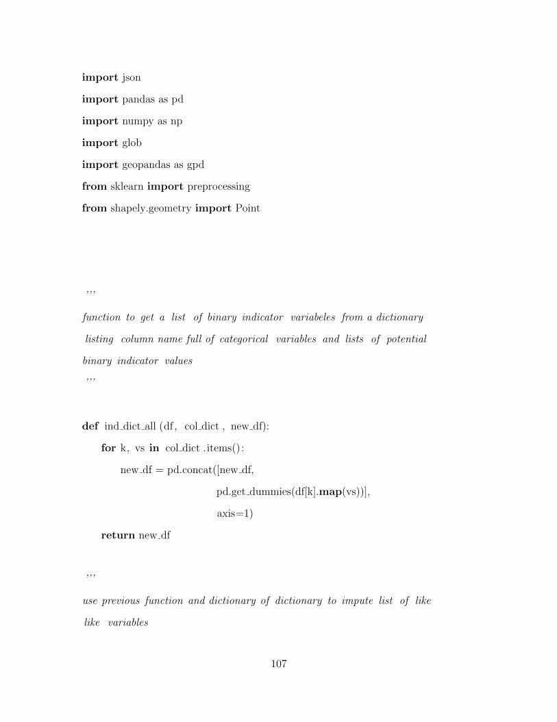
import json

import pandas as pd

import numpy as np

import glob

import geopandas as gpd

from sklearn import preprocessing

from shapely.geometry import Point

’’’

function to get a list of binary indicator variabeles from a dictionary

listing column name full of categorical variables and lists of potential

binary indicator values

’’’

def ind dict all (df , col dict , new df):

for k, vs in col dict .items():

new df = pd.concat([new df,

pd.get dummies(df[k].map(vs))],

axis=1)

return new df

’’’

use previous function and dictionary of dictionary to impute list of like

like variables

107

’’’

def indicator variables dict all (database, dictionary ,new database):

for key in dictionary :

new database = (pd.concat([new database,

pd.get dummies(database[key].map(

dictionary [key])) ], axis = 1))

return new database

#Not really used

def single binary(database,

column name,

one value,

zero value ,

new name,

new database):

lst = []

for i in database[column name]:

if i == one value:

lst .append(1)

else:

lst .append(0)

bin col = pd.DataFrame(new name:lst)

new database = pd.concat([new database, bin col], axis = 1)

return new database

’’’

108

Reduces a list of colums relating to multiple variables dealing with the same

subject matter into two variables − one coninuous and the other binary.

Used for variables like DELDOC (number of kids delivered by a doctor in past

3−5 years) which allows for up to 6 kids to indicate as either yes (1) or

no (0) or not related (8, 9, or NaN)

’’’

def mult bin cont(df, col lst , new df):

cond num = [] #numeric col for # of whatever variable measuring

nan obs = [8, 9]

sub df = df[ col lst ]. replace(nan obs,np.NaN) #NIU & missing = nan

for col in col lst : # if true for one child

cond num.append(sub df[col] ==1)

#num of kids who were delivered by doctor

col num = pd.Series((np.where(cond num, 1, 0)).transpose().sum(axis=1))

#doesn’t have kids, answered or questions not asked

col nan = pd.Series((np.where(

sub df. isnull () . all(axis=1), 1, 0)) .transpose())

col num.index = sub df.index #making indes the same for concat

col nan.index = sub df.index

sub df new = pd.concat([col num.rename(col lst[0].lower() . split ( ’ ’ ) [0]

+’ num’),

col nan.rename(col lst [0]. lower() . split ( ’ ’ ) [0]

+ ’ na’) ],

axis = 1)

#normalize based on wether not you had a kid delivered

109

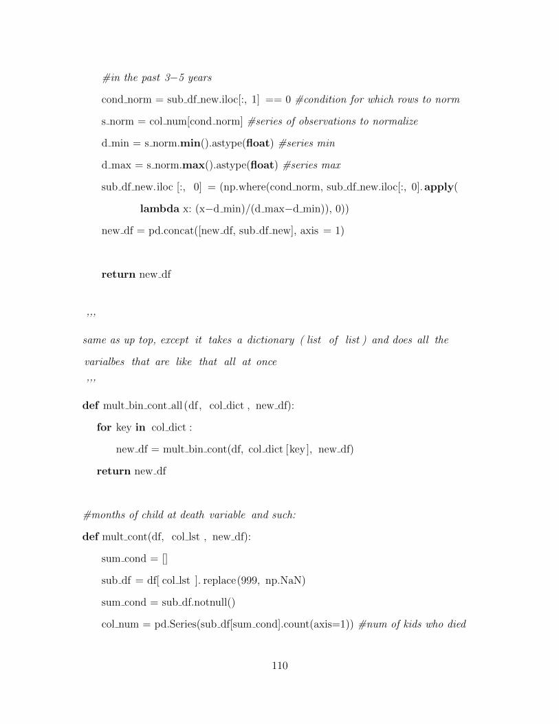
#in the past 3−5 years

cond norm = sub df new.iloc[:, 1] == 0 #condition for which rows to norm

s norm = col num[cond norm] #series of observations to normalize

d min = s norm.min().astype(float) #series min

d max = s norm.max().astype(float) #series max

sub df new.iloc [:, 0] = (np.where(cond norm, sub df new.iloc[:, 0].apply(

lambda x: (x−d min)/(d max−d min)), 0))

new df = pd.concat([new df, sub df new], axis = 1)

return new df

’’’

same as up top, except it takes a dictionary ( list of list ) and does all the

varialbes that are like that all at once

’’’

def mult bin cont all (df , col dict , new df):

for key in col dict :

new df = mult bin cont(df, col dict [key], new df)

return new df

#months of child at death variable and such:

def mult cont(df, col lst , new df):

sum cond = []

sub df = df[ col lst ]. replace(999, np.NaN)

sum cond = sub df.notnull()

col num = pd.Series(sub df[sum cond].count(axis=1)) #num of kids who died

110

#its ignoring NaN values and finding mean number of months at dealth

month num = sub df.mean(axis=1)

col nan = pd.Series((np.where(sub df. isnull () . all(axis=1),

1, 0)) .transpose()) #no kids died

col nan.index = col num.index

sub df new = pd.concat([col num.rename(col lst[0].lower() . split ( ’ ’ ) [0]

+ ’ num’),

col nan.rename(col lst [0]. lower() . split ( ’ ’ ) [0]

+ ’ nan’),

month num.rename(col lst[0].lower(). split ( ’ ’ ) [0]

+ ’ mean month’)],

axis = 1)

#normalize

cond norm = sub df new.iloc[:, 1] == 0

#series of number of children to normalize

s norm num = col num[cond norm]

#series of mean age (months) to normalize

s norm month = month num[cond norm]

#getting appropriate min and max for nomralization

num max = s norm num.max()

num min = s norm num.min()

month max = s norm month.max()

month min = s norm month.min()


111

lambda x: (x−num min)/(num max−num min)), 0))


lambda x: (x−month min)/(month max−month min)), 0))

new df = pd.concat([new df, sub df new], axis=1)

return new df

’’’

normalizing function for varaibles with mainly continuous values but

does contain some categorical values

’’’

def min max normalize(df, col):

col norm = (df[col ] − df[col ]. min())/ (df[col ]. max() − df[col].min())

return col norm

def min max normalize lst(df, col lst , new df):

nan lst = [95, 96, 97, 98, 99]

sub df = df[ col lst ]. replace(nan lst , np.NaN)

for col in sub df:

if sub df[ col ]. isnull () .any():

#indicator variable for missing values as this dataset ’s

#null values carry meaning −

#ex.) age1stbirth == NaN means that women hasn’t had child yet.

112

col nan = pd.Series((np.where(

sub df[ col ]. isnull () , 1, 0)) .transpose())

col num = min max normalize(sub df, col)

#adding one to every obs−shift continuous spread

col num = col num.apply(lambda x: x+1)

col num = col num.fillna(0)#replacing NaN’s with 0

col nan.index = sub df.index

col num.index = sub df.index


col nan.rename(col.lower() + ’ nan’),

col num.rename(col.lower() + ’ norm’)],

axis = 1)

else:

col num = min max normalize(df, col)

#making normal scale equal for every cont. variable

col num = col num.apply(lambda x: x+1)

col num.index = sub df.index


col num.rename(col.lower() + ’ norm’)],

axis = 1)

return new df

113

’’’

normalizing functions for strictly continuous varaibles

’’’

def normalize cont(df,

col lst ,

new df):

sub array = df[ col lst ]. fillna (0) .values

min max scaler = preprocessing.MinMaxScaler()

array scaled = min max scaler.fit transform(sub array)

norm lst = []

for i in col lst :

norm lst.append(i.lower() + ’ norm’)

sub df = pd.DataFrame(data = array scaled,

index = new df.index,

columns = norm lst)

new df = pd.concat([new df, sub df], axis = 1)

return new df

’’’

Load and combine geodataframes

’’’

114

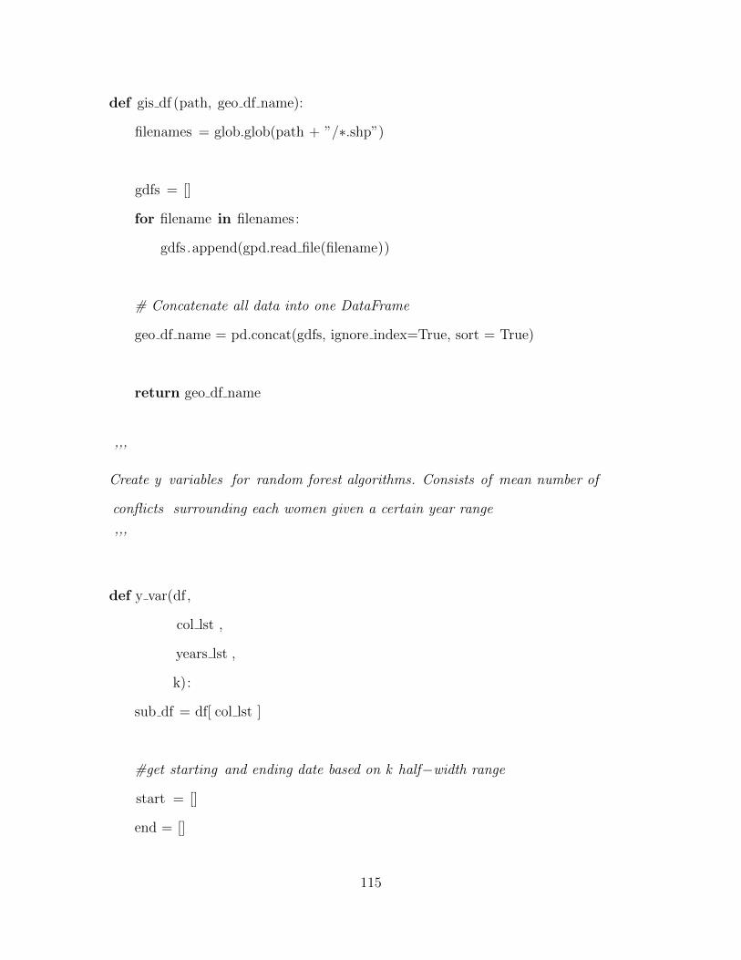
def gis df (path, geo df name):

filenames = glob.glob(path + ”/∗.shp”)

gdfs = []

for filename in filenames:

gdfs .append(gpd.read file(filename))

# Concatenate all data into one DataFrame

geo df name = pd.concat(gdfs, ignore index=True, sort = True)

return geo df name

’’’

Create y variables for random forest algorithms. Consists of mean number of

conflicts surrounding each women given a certain year range

’’’

def y var(df ,

col lst ,

years lst ,

k):

sub df = df[ col lst ]

#get starting and ending date based on k half−width range

start = []

end = []

115

for i in df[ ’INTYEAR’]:

start .append(int(i − k))

end.append(int(i + k))

#convert to pd.series and make sure every one has the same indicies

start = pd.Series(start)

start .index = df.index

end = pd.Series(end)

end.index = df.index

violence bool = []

for i in years lst :

violence bool .append((i >= start) & (i <= end))

violence bool = pd.DataFrame(violence bool).transpose()

violence mean = pd.DataFrame(np.where(violence bool,

sub df.values ,

np.NaN)).mean(axis = 1)

#violence mean = np.array(violence mean)

return violence mean

116

#

#############################################################################

#Make dataframe into GeoDataFrame with geometry point ’clust coord’

def df to gdf(df) :

df [ ’ clust coord ’ ] = list(zip(df.LONGNUM, df.LATNUM))

df [ ’ clust coord ’ ] = df[’ clust coord ’ ]. apply(Point)

gdf = gpd.GeoDataFrame(df, geometry = ’clust coord’)

return gdf

#Function that returns a geodataframe for a group in the THD based on the

#json files from the Segmentations Folder

def group gdf(gdf, #GeoPandas Dataframe already loaded

thd path, #Path to THD

json file name #String indicating file name

) :

#The json file

json file = THD PATH + json file name

#Empty Dictionary to hold json file

117

CONFIG PROPERTIES =

try:

with open(json file) as data file :

CONFIG PROPERTIES = json.load(data file)

except IOError as e:

print(e)

exit ()

#list of rows in the THD group − will be used to create a subset of

#the larger whole dataset attributed

row indices = CONFIG PROPERTIES[’rows’]

#Geo Dataframe of data in Subgroup

sub gdf = gdf. iloc [ row indices , :]

return sub gdf

#

###########################################################################

’’’

a function to grab a bunch of nodes from a list that I will define

based on anlysis from some simplicial complex created through TDA

that that statistical analysis can be implimented on it later on

118

UPDATE: Switched to Ayasdi from kmapper − thses functions are no longer

relavant but potentially useful if you want to use kmapper.

Just add kmapper and respective libraries to run

’’’

’’’

def grab cluster group ( lst , array, scomplex):

cluster grouping = np.empty((0,array.shape[1]), float )

for i in lst :

cluster grouping = np.append(cluster grouping,

mapper.data from cluster id(i ,

scomplex,

array),

axis = 0)

cluster grouping unique = np.unique(cluster grouping, axis = 0)

return cluster grouping unique

def grab clusters id ( lst , array index, scomplex):

clusters id = []

for i in lst :

clusters id = np.append(clusters id,

mapper.data from cluster id(i ,

scomplex,

119

array index),

axis = 0)

unique id = np.unique(clusters id , axis = 0)

return unique id

’’’

120

Appendix D. Data Cleaning and Manipulation Code

The following code was used to clean and manipulate the data before impliment-

ing Topological Data Analysis through Ayasdi Software and Geospatial Analysis in

Python Jupyter Notebooks.

The following Python packages were utilized in the code below.

• numpy >= 1.15.2 [78]

• sys [66]

• glob [66]

• pandas >= 0.23.4 [76]

• numpy >= 1.15.2 [78]

• geopandas >= 0.4.0 [67]

• sklearn >= 0.0 [77]

• matplotlib >= 3.0.2 [79]

# −∗− coding: utf−8 −∗−

”””

Created on Wed Oct 10 14:42:34 2018

@author: Michaela

”””

#

############################################################################

121

#Libraries imported

import sys

import pandas as pd

import numpy as np

import geopandas as gpd

import glob

import matplotlib.pyplot as plt

from sklearn.model selection import train test split

from sklearn import preprocessing

from sklearn.ensemble import RandomForestRegressor

from sklearn import ensemble

from sklearn.metrics import mean squared error

import thesis functions as func #importing functions for data manipulation

import thesis dictionaries as dic #import dictionaries and lists for data manip

#Path to datafile − change depending on whoes using script

path = (’C:\\Users\\Michaela\\Documents\\Thesis’ +

’\\Data−Code\\Data final\\Manipulation\\’)

#ˆˆ had to put on two lines due to length and fitting in appendix

#Load csv datafile as pandas DataFrame

df= pd.read csv(path+’women conflict.csv’)

’’’

Drop all observation before the year 1997 due to conflict data restrictions ,

122

And replace −998 (DHS survey doesn’t have GPS locations) with NaN so that

I can drop them

’’’

df = df.drop(df[df .YEAR < 1997].index)

df = df.replace(−998, np.NaN)

conflict cond = (df[ ’CIV VIOLENCE 1997’].notnull())

df = df[ conflict cond ] #getting rid of observations are Nan

#Country abreviation (first two letters ) + year (YYYY) − 33 samples

#helps with data cleaning process , but not really used after

df[ ’ID’] = df.DHSID.str[:6]

df .ID.astype(’category’)

df [ ’COUNTRY’] = df[’COUNTRY’].map(dic.country dict)

’’’

Create the DataFrame that will be exported out for Analysis and add variables

that can be transported as is − see dictionaries .py for list

’’’

df tda = []

for col in dic . as is lst :

df tda.append(list(df[col ]) )

df tda = pd.DataFrame(df tda).transpose()

df tda.columns = dic. as is lst

df tda.index = df.index #have to make sure indicies match up for later

123

’’’

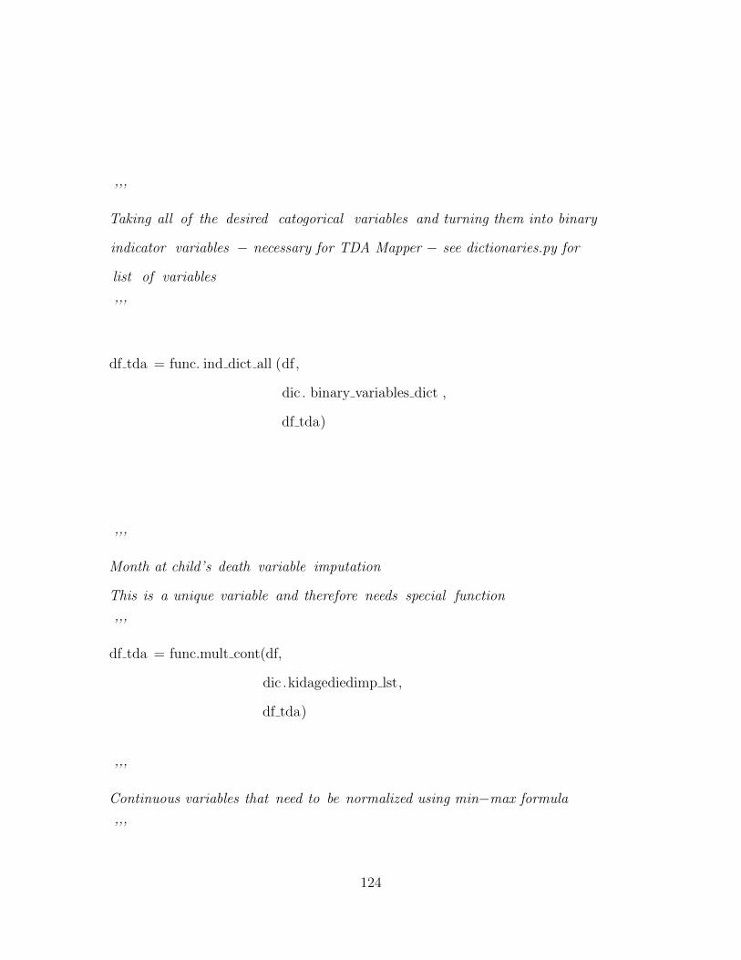
Taking all of the desired catogorical variables and turning them into binary

indicator variables − necessary for TDA Mapper − see dictionaries.py for

list of variables

’’’

df tda = func. ind dict all (df ,

dic . binary variables dict ,

df tda)

’’’

Month at child’s death variable imputation

This is a unique variable and therefore needs special function

’’’

df tda = func.mult cont(df,

dic .kidagediedimp lst,

df tda)

’’’

Continuous variables that need to be normalized using min−max formula

’’’

124

df tda = func.min max normalize lst(df,

dic .norm lst,

df tda)

’’’

HHEADAGE has different missing values so it has to be normalized by itself

’’’

hheadage norm = func.min max normalize(df, ’HHEADAGE’)

hheadage norm = hheadage norm.apply(lambda x: x+1) #same as other cont.

vars.

df tda = pd.concat([df tda, hheadage norm], axis=1)

’’’

Variables like DELDOC that make up several variables that relate to each

potential mothers multiple children that could have been in the past 3−5 years

will be composed of two variables, one with a normalized number relateding to

the number and another indicator variable indicating if the women belongs in

universe (meaning the women can provide a meaning fule answer, i.e. I had

a baby in the past five years therefore I can answer a question pertaining

to my prenatal care and so on).

’’’

df tda = func.mult bin cont all(df ,

dic . bin cont dict ,

125

df tda)

’’’

Add on riots, battles and civ violence variables

’’’

#get predictor values − based of off 2 year half width

y riots = func.y var(df, dic . riots lst , dic . violence yr lst , 2)

y civ = func.y var(df, dic . civ violence lst , dic . violence yr lst , 2)

y battles = func.y var(df, dic . battles lst , dic . violence yr lst , 2)

list of lists = [y riots , y battles , y civ ]

y all = [sum(x) for x in zip(∗ list of lists ) ]

y riots .index = df tda.index

y civ .index = df tda.index

y battles .index = df tda.index

y all = pd.Series( y all , index = df tda.index)

bin riots = y riots .apply(lambda x: 1 if x > 0 else 0)

bin civ = y civ.apply(lambda x: 1 if x > 0 else 0)

bin battles = y battles.apply(lambda x: 1 if x > 0 else 0)

bin all = y all .apply(lambda x: 1 if x > 0 else 0)

’’’

Add to dataframe for latter csv extractions

126

’’’

’’’

Add on riots, battles and civ vi0lence variables normalized (lower case)

’’’

df = df. fillna (0) #just for the Riots 2008 (Niger 1998 sample data mix−up)

df tda = func.normalize cont(df,

dic . violence cols ,

df tda)

’’’

Anomaly Detection using Isolation Forest and data with both Violence data and

no violence data − i.e. only women survey data

’’’

var names = list(df tda) #get list to determine X violence and X women

X violence = df tda. iloc [:, 4:427]. values #Take away DHSID, country, ect.

X women = df tda.iloc[:, 4:367]. values #Take away violence data

#Isolation Forest using Bootstrap sampling

model = ensemble.IsolationForest(bootstrap = True,

random state=123,

max samples = 25)

model.fit (X violence)#Fiting model to data

lens violence = model.decision function(X violence) #Getting anomaly scores

127

model.fit (X women)#Fiting model to data

lens women = model.decision function(X women)#Getting anomaly scores

#Convert numpy arrays to series so that they can be added to dataframe

anomaly violence = pd.Series(lens violence , index = df tda.index)

anomaly women = pd.Series(lens women, index = df tda.index)

#Add everything to data frame

df tda = pd.concat([df tda,

y riots .rename(’y riots ’ ) ,

bin riots .rename(’bin riots ’ ) ,

y civ .rename(’y civ’) ,

bin civ .rename(’bin civ’) ,

y battles .rename(’y battles’) ,

bin battles .rename(’bin battles’ ) ,

y all .rename(’y all ’ ) ,

bin all .rename(’bin all ’ ) ,

anomaly violence.rename(’anomaly violence’),

anomaly women.rename(’anomaly women’)],

axis = 1)

#Anomaly scores distributions plot

bins = np.linspace(−0.2, 0.2, 500)

plt . hist ( lens violence , bins, alpha=0.5,

128

label=’Augmented Women and Conflict Data’)

plt . hist (lens women, bins, alpha=0.5,

label=’DHS Women Survey Answers Only’)

plt .legend(loc=’upper right’)

plt . ylabel( ’Frequency’)

plt . xlabel( ’ Isolation Forest Anamoly Score’)

plt . title ( ’ Isolation Forest Anamoly Scores Histograms’)

plt .show()

#get list to determine X

var names = list(df tda)

’’’

get Random Forest predicted values for violence using sklearn and convert

data to numpy arrays (or just use origional numpy arrays)

’’’

X = df tda.iloc [:, 4:367]. values

X t, X v, y r t , y r v , y b t , y b v, y c t , y c v, y a t , y a v =

train test split (

X, y riots , y battles , y civ , y all , test size =0.25, random state=123)

’’’

Build Regression Radom Forest Tree for lenses for each Y variable with

bootstrap sampling

’’’

129

reg = RandomForestRegressor(bootstrap = True,

random state=123,

n estimators = 75)

#riots lens

reg. fit (X t, y r t )

riots pred test = reg.predict(X v)

riots mse = mean squared error(y r v, riots pred test )

riots score = reg.score(X v, y r v)

lens pred riots = reg.predict(X)

#battles random forest regression lens

reg. fit (X t, y b t)

battles pred test = reg.predict(X v)

battles mse = mean squared error(y b v, battles pred test)

battles score = reg.score(X v, y b v)

lens pred battles = reg.predict(X)

#civ violence random forest regression lens

reg. fit (X t, y c t)

civ pred test = reg.predict(X v)

civ mse = mean squared error(y c v, civ pred test)

civ score = reg.score(X v, y c v)

130

lens pred civ = reg.predict(X)

#all violence acts random forest regression lens

reg. fit (X t, y a t)

all pred test = reg.predict(X v)

all mse = mean squared error(y a v, all pred test )

all score = reg.score(X v, y a v)

lens pred all = reg.predict(X)

lens pred riots = pd.Series( lens pred riots )

lens pred battles = pd.Series( lens pred battles )

lens pred civ = pd.Series( lens pred civ )

lens pred all = pd.Series( lens pred all )

#Add new lenses onto the dataframe to be loaded up into Ayasdi

df lens = pd.concat([ lens pred riots .rename(’riot lens ’ ) ,

lens pred battles .rename(’battles lens ’ ) ,

lens pred civ .rename(’ civ violence lens ’ ) ,

lens pred all .rename(’ violence all lens ’ ) ],

axis = 1)

df lens .index = df tda.index

131

df tda = pd.concat([df tda, df lens ], axis = 1)

#Load in absolute difference between predicted and actual

riots diff = pd.Series(( y riots − lens pred riots ) .abs(), index = df tda.index)

battles diff = pd.Series((y battles − lens pred battles) .abs(), index = df tda.

index)

civ diff = pd.Series((y civ − lens pred civ) .abs(), index = df tda.index)

violence all diff = pd.Series(( y all − lens pred civ) .abs(), index = df tda.index

)

df diff = pd.concat([ riots diff .rename(’ riots diff ’ ) ,

battles diff .rename(’ battles diff ’ ) ,

civ diff .rename(’ civ diff ’ ) ,

violence all diff .rename(’ violence all diff ’ ) ], axis = 1)

df diff .index = df tda.index

df tda = pd.concat([df tda, df diff ], axis = 1)

’’’

Geopandas GIS data

’’’

#Reading in all shape files loaded from DHS Program website and concat together

gdf = func.gis df (path + ’shps\\’, ’gdf’ )

132

gdf sub = gdf[[ ’LATNUM’, ’LONGNUM’, ’geometry’]]

df tda = pd.merge(df tda, gdf[[ ’DHSID’, ’LATNUM’, ’LONGNUM’]], on = ’

DHSID’)

path analysis = (’C:\\Users\\Michaela\\Documents\\Thesis\\Data−Code’ +

’\\Data final\\Analysis\\’) #Too long and went of page

df tda. to csv(path analysis + ’analysis data .csv’)

133

Appendix E. Jupyter Notebook Analysis

The following Jupyter Notebook output summarizes all geospatial analysis impli-

mented.

The following Python packages were utilized in the code below.

• numpy >= 1.15.2 [78]

• sys [66]

• os [66]

• glob [66]

• pandas >= 0.23.4 [76]

• numpy >= 1.15.2 [78]

• geopandas >= 0.4.0 [67]

• geoplot >= 0.2.1 [68]

• seaborn >= 0.9.0 [81]

• sklearn >= 0.0 [77]

• matplotlib >= 3.0.2 [79]

134

Geospatial Analysis

In [2]: import os import sys import glob import numpy as np import json import pandas as pd import geopandas as gpd import geoplot as gplt import thesis_functions as func import thesis_dictionaries as dic from shapely.geometry import Point import matplotlib.pyplot as plt import geoplot.crs as gcrs

In [3]: #Segmentation Folder path THD1_path = ('C:\\Users\\Michaela\\Desktop\\AFRL\\Segmentations\\' +

'N1N2_IQR_WomenData(2)_IQR Normalized Euclidean_analysis_data_6.csv 2_2018.12.14 16.20.58\\')

THD2_path = ('C:\\Users\\Michaela\\Desktop\\AFRL\\Segmentations\\' + 'ALL_N1N2_IQR_IQR Normalized Euclidean_analysis_data_6.csv 2_2019.

01.10 17.53.40\\')

#Data File path path = 'C:\\Users\\Michaela\\Documents\\Thesis\\Data-Code\\Data_final\\Analysis\\'

In [4]: #Grab the list of json files that will be used to index data from segmentationfolder files = [i for i in os.listdir(THD1_path) if os.path.isfile(os.path.join(THD1_path,i)) and \

'GROUPDATA_' in i]

print(len(files)) #if correctly done, should only be 137

137

135

Geospatial Analysis

In [5]: #read Pandas DataFrame used for the Analysis df = pd.read_csv(path + 'analysis_data_6.csv') print(df.shape) df.head()

In [6]: #Unnamed columns was column added when reading out dataframe to csv after manipulation, so I'm going to get rid of it df = df.drop(['Unnamed: 0'], axis = 1) df.head()

In [7]: #read in shape files and merge with DataFrame on the DHS Cluster ID number tomake a geodataframe

path_shps = 'C:\\Users\\Michaela\\Documents\\Thesis\\Data-Code\\Data_final\\Manipulation\\shps\\' gdf_survey = func.gis_df(path_shps, 'gdf') df = pd.merge(df, gdf_survey[['DHSID', 'geometry']], on = 'DHSID') gdf_full = gpd.GeoDataFrame(df, geometry = 'geometry')

(255221, 448)

Out[5]:

Unnamed:0 DHSID CLUSTERNO COUNTRY INTYEAR WEALTHS Anglican Animist

0 0 BJ200100000001 1 Benin 2001 -0.22614 0 0

1 1 BJ200100000001 1 Benin 2001 -0.22614 0 0

2 2 BJ200100000001 1 Benin 2001 -0.40480 0 0

3 3 BJ200100000001 1 Benin 2001 -0.40480 0 0

4 4 BJ200100000001 1 Benin 2001 -0.46920 0 0

5 rows × 448 columns

Out[6]:

DHSID CLUSTERNO COUNTRY INTYEAR WEALTHS Anglican Animist Catholic

0 BJ200100000001 1 Benin 2001 -0.22614 0 0 0

1 BJ200100000001 1 Benin 2001 -0.22614 0 0 0

2 BJ200100000001 1 Benin 2001 -0.40480 0 0 0

3 BJ200100000001 1 Benin 2001 -0.40480 0 0 0

4 BJ200100000001 1 Benin 2001 -0.46920 0 0 0

5 rows × 447 columns

136

Geospatial Analysis

In [8]: #So that I can graph later on gdf_full.crs = 'init' :'epsg:4326'

Load borders and cities geodataframes for graphing purposes

In [9]: #Load borders shape file from thematicmapping.org borders = gpd.read_file(path + 'TM_WORLD_BORDERS-0.3.shp') #Uploading world cities shape file - downloaded from ARCGIS Hub website cities = gpd.read_file(path + 'World_Cities.shp') #plot base = borders.plot(color = 'white', edgecolor = 'black') cities.plot(ax=base, marker='o', color='red', markersize=1)

In [10]: #reduce the borders and cities geodataframe to hold the 9 countries of interest with cities country_list = ['Benin', 'Ghana', 'Nigeria', 'Niger', 'Guinea', 'Burkina Faso', 'Cameroon', 'Mali', 'Cote d\'Ivoire'] borders = borders[borders['NAME'].isin(country_list)] cities = cities[cities['CNTRY_NAME'].isin(country_list)] #plot base = borders.plot(color = 'white', edgecolor = 'black') cities.plot(ax=base, marker='o', color='red', markersize=5)

Out[9]: <matplotlib.axes._subplots.AxesSubplot at 0x1c607943780>

Out[10]: <matplotlib.axes._subplots.AxesSubplot at 0x1c607122828>

137

Geospatial Analysis

In [11]: #only look at realy large cities so as to lessen the information on the map large_cities_lst = [ '1,000,000 to 4,999,999', '5,000,000 and greater'] #cities with 1million or more population cities_large = cities[cities['POP_CLASS'].isin(large_cities_lst)] #plot base = gplt.polyplot(borders) gplt.pointplot(cities_large,ax=base, color='red') plt.savefig("bage.jpg", bbox_inches='tight', pad_inches=0.1)

Initial Geospatial Analysis

Looking at certain indicators that are believed to be determinants of well-being, particularly: educationLiteracyFGMConflict

138

Geospatial Analysis

In [12]: #Education = none: points = gdf_full[gdf_full['edachiever_none'] == 1] #only have points that represent women with no education #Kernal density map showing where the women with no education are densest print(points.shape)

ax = gplt.kdeplot(points, shade=True, shade_lowest=False, clip=borders.geometry)

base_borders = gplt.polyplot(borders, ax=ax) base_cities = cities_large.plot(ax = ax, marker='o', color='red', markersize=10)

plt.savefig("edu_none_KLD_map.jpg", bbox_inches='tight', pad_inches=0.1)

C:\Users\Michaela\AppData\Roaming\Python\Python37\site-packages\scipy\stats\stats.py:1713: FutureWarning: Using a non-tuple sequence for multidimensional indexing is deprecated; use àrr[tuple(seq)]` instead of àrr[seq]`. In the future this will be interpreted as an array index, àrr[np.array(seq)]`, which will result either in an error or a different result. return np.add.reduce(sorted[indexer] * weights, axis=axis) / sumval

(131572, 448)

139

Geospatial Analysis

In [13]: #education = higher: points = gdf_full[gdf_full['edachiever_higher'] == 1] #only have points that represent women with some form of higher edu #Kernal density map showing where the women with higher education are densest print(points.shape)



plt.savefig("edu_higher_KLD_map.jpg", bbox_inches='tight', pad_inches=0.1)

(10137, 448)


140

Geospatial Analysis

In [13]: #FGM = yes: points = gdf_full[gdf_full['fccirc_yes'] == 1] #Kernal density map showing where women are circumcised are densest print(points.shape)



plt.savefig("fgm_yes_KLD_map.jpg", bbox_inches='tight', pad_inches=0.1)


141

Geospatial Analysis

In [15]: #Conflict variables box plots import seaborn as sns conflict = pd.DataFrame(gdf_full[['y_riots', 'y_battles', 'y_civ']]) ax = sns.boxplot(x = "variable", y="value", data=pd.melt(conflict)) plt.savefig("conflict_boxplots.jpg")

In [16]: ax = sns.boxplot(conflict.y_riots, color = 'red') ax.set(xlabel='Riots') plt.savefig("riots_boxplot.jpg") plt.show() print(conflict.y_riots.describe())

count 255221.000000 mean 5.511230 std 13.678973 min 0.000000 25% 0.000000 50% 0.000000 75% 5.600000 max 149.400000 Name: y_riots, dtype: float64

142

Geospatial Analysis

In [17]: ax = sns.boxplot(conflict.y_battles, color = 'green') ax.set(xlabel='Battles') plt.savefig("battles_boxplot.jpg") plt.show() print(conflict.y_battles.describe())

count 255221.000000 mean 1.101642 std 2.662744 min 0.000000 25% 0.000000 50% 0.000000 75% 1.200000 max 44.200000 Name: y_battles, dtype: float64

143

Geospatial Analysis

In [18]: ax = sns.boxplot(conflict.y_civ, color = 'blue') ax.set(xlabel='Civilian Violence') plt.savefig("civ_boxplot.jpg") plt.show() print(conflict.y_civ.describe())

count 255221.000000 mean 1.729243 std 3.740114 min 0.000000 25% 0.000000 50% 0.000000 75% 2.200000 max 64.000000 Name: y_civ, dtype: float64

144

Geospatial Analysis

In [19]: #Riots _bin_all: points = gdf_full[gdf_full['bin_riots'] == 1] print(points.shape) ax = gplt.kdeplot(points,

shade=True, shade_lowest=False, clip=borders.geometry)


plt.savefig("bin_riots_KLD_map.jpg", bbox_inches='tight', pad_inches=0.1)


145

Geospatial Analysis

In [20]: #Riots_bin_greater than 5.6 - only looking at extreme conflict in riots (5.6 =75% in riots) points = gdf_full[gdf_full['y_riots'] > 5.6] print(points.shape)



plt.savefig("extreme_riots_KLD_map.jpg", bbox_inches='tight', pad_inches=0.1)

(63720, 448)


146

Geospatial Analysis

In [21]: #battles: points = gdf_full[gdf_full['bin_battles'] == 1]



plt.savefig("bin_battles_KLD_map.jpg", bbox_inches='tight', pad_inches=0.1)


147

Geospatial Analysis

In [22]: #battles_greater than 1.2 - only looking at extreme conflict in battles (1.2 =75% in battles) points = gdf_full[gdf_full['y_battles'] > 1.2] print(points.shape)



plt.savefig("extreme_battles_KLD_map.jpg", bbox_inches='tight', pad_inches=0.1)

(56637, 448)


148

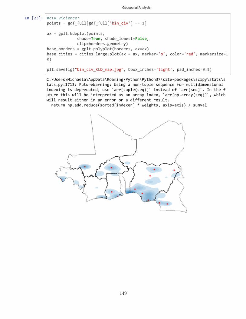
Geospatial Analysis

In [23]: #civ_violence: points = gdf_full[gdf_full['bin_civ'] == 1]



plt.savefig("bin_civ_KLD_map.jpg", bbox_inches='tight', pad_inches=0.1)


149

Geospatial Analysis

In [24]: #civ_greater than 2.2 - only looking at extreme conflict in civilian violence(2.2 = 75%) points = gdf_full[gdf_full['y_civ'] > 2.2] print(points.shape)



plt.savefig("extreme_civ_KLD_map.jpg", bbox_inches='tight', pad_inches=0.1)

(59695, 448)


150

Geospatial Analysis

In [25]: #Anomalous Women points = gdf_full[gdf_full['anomaly_women'] < 0] print(points.shape) ax = gplt.kdeplot(points,



plt.savefig("anomalous_women_KLD_map.jpg", bbox_inches='tight', pad_inches=0.1)

(7786, 448)


151

Geospatial Analysis

In [27]: #Anomalous_violence Graph points = gdf_full[gdf_full['anomaly_violence'] < 0] ax = gplt.kdeplot(points,



plt.savefig("anomalous_violence_KLD_map.jpg", bbox_inches='tight', pad_inches=0.1) print(points.shape)

THD Geospatial Analysis

Obtaining sub-dataframes from the main dataframe based on the THD and then holding them in a dictionary thatcan be called by THD name


(424, 448)

152

Geospatial Analysis


'GROUPDATA_' in i]

print(len(files)) #if correctly done, should only be 137

#Dictionary holding all of THD1's GeoDataFrames groups gdfs1 = #Starting empty dictionary

# Got this code from this youtube video: https://www.youtube.com/watch?v=hZNeKPZRPdM for file in files: group_name = file.split(' ')[1][:-5].replace('.', '_') #get group number i

n format of #_#_# dataframe_name = 'gdf' + '_' + group_name #example = gdf_25_1_0 json_file = THD1_path + file

#Empty Dictionary to hold json file CONFIG_PROPERTIES = try:

with open(json_file) as data_file: CONFIG_PROPERTIES = json.load(data_file)

except IOError as e: print(e) exit(1)

#list of rows in the THD group - will be used to create a subset of #the larger whole dataset attributed row_indices = CONFIG_PROPERTIES['rows']

#Geo Dataframe of data in Subgroup gdfs1[dataframe_name] = gdf_full.iloc[row_indices, :]

#checking for gdf in gdfs1: print(gdf), print(gdfs1[gdf].shape)

153

Geospatial Analysis

137 gdf_0_0_0 (255221, 448) gdf_1_0_0 (255221, 448) gdf_10_0_0 (177558, 448) gdf_10_1_1 (201, 448) gdf_10_7_2 (8633, 448) gdf_10_7_3 (6264, 448) gdf_10_7_4 (4225, 448) gdf_10_7_5 (1913, 448) gdf_10_7_6 (288, 448) gdf_10_7_7 (259, 448) gdf_10_8_10 (127, 448) gdf_10_8_8 (11761, 448) gdf_10_8_9 (4301, 448) gdf_10_9_11 (264, 448) gdf_10_9_12 (204, 448) gdf_10_9_13 (168, 448) gdf_10_9_14 (151, 448) gdf_11_0_0 (176065, 448) gdf_11_2_1 (835, 448) gdf_11_2_10 (183, 448) gdf_11_2_2 (545, 448) gdf_11_2_3 (485, 448) gdf_11_2_4 (396, 448) gdf_11_2_5 (330, 448) gdf_11_2_6 (324, 448) gdf_11_2_7 (200, 448) gdf_11_2_8 (185, 448) gdf_11_2_9 (185, 448)

154

Geospatial Analysis

gdf_11_3_11 (776, 448) gdf_11_3_12 (482, 448) gdf_11_3_13 (159, 448) gdf_11_3_14 (106, 448) gdf_11_3_15 (100, 448) gdf_11_4_16 (103, 448) gdf_11_8_17 (3460, 448) gdf_11_8_18 (2576, 448) gdf_11_8_19 (890, 448) gdf_11_8_20 (834, 448) gdf_11_8_21 (195, 448) gdf_11_8_22 (181, 448) gdf_11_8_23 (119, 448) gdf_11_9_24 (176, 448) gdf_12_0_0 (173792, 448) gdf_13_0_0 (171695, 448) gdf_14_0_0 (168693, 448) gdf_14_0_1 (235, 448) gdf_14_0_2 (202, 448) gdf_15_0_0 (163016, 448) gdf_15_0_1 (199, 448) gdf_15_0_2 (104, 448) gdf_16_0_0 (157204, 448) gdf_16_0_1 (176, 448) gdf_17_0_0 (151749, 448) gdf_17_0_1 (411, 448) gdf_17_0_2 (252, 448) gdf_17_0_3 (120, 448) gdf_18_0_0

155

Geospatial Analysis

(147444, 448) gdf_19_0_0 (141533, 448) gdf_19_0_1 (565, 448) gdf_19_0_2 (506, 448) gdf_19_0_3 (235, 448) gdf_2_0_0 (197763, 448) gdf_2_0_1 (57458, 448) gdf_20_0_0 (106845, 448) gdf_20_0_1 (25348, 448) gdf_20_0_2 (2386, 448) gdf_20_0_3 (1256, 448) gdf_20_0_4 (1070, 448) gdf_20_0_5 (578, 448) gdf_21_0_0 (91627, 448) gdf_21_0_1 (376, 448) gdf_21_0_2 (166, 448) gdf_21_0_3 (159, 448) gdf_21_0_4 (122, 448) gdf_21_0_5 (110, 448) gdf_21_1_10 (219, 448) gdf_21_1_11 (188, 448) gdf_21_1_12 (185, 448) gdf_21_1_13 (102, 448) gdf_21_1_6 (4100, 448) gdf_21_1_7 (3302, 448) gdf_21_1_8 (853, 448) gdf_21_1_9 (408, 448) gdf_22_0_0 (79438, 448) gdf_23_0_0 (65054, 448)

156

Geospatial Analysis


157

Geospatial Analysis

(57055, 448) gdf_6_0_0 (181241, 448) gdf_6_1_1 (15864, 448) gdf_6_2_2 (56433, 448) gdf_7_0_0 (180925, 448) gdf_7_1_1 (14748, 448) gdf_7_2_2 (54941, 448) gdf_8_0_0 (180193, 448) gdf_8_1_1 (7956, 448) gdf_8_1_2 (2703, 448) gdf_8_1_3 (1392, 448) gdf_8_1_4 (575, 448) gdf_8_1_5 (150, 448) gdf_8_2_6 (53056, 448) gdf_9_0_0 (179247, 448) gdf_9_1_1 (2303, 448) gdf_9_1_2 (1504, 448) gdf_9_1_3 (1097, 448) gdf_9_1_4 (888, 448) gdf_9_2_5 (166, 448) gdf_9_2_6 (124, 448) gdf_9_6_7 (24524, 448) gdf_9_6_8 (19993, 448) gdf_9_6_9 (5204, 448)

158

Geospatial Analysis


'GROUPDATA_' in i]

#Dictionary holding all of THD2's GeoDataFrames groups gdfs2 = #Starting empty dictionary

# Got this code from this youtube video: https://www.youtube.com/watch?v=hZNeKPZRPdM for file in files: group_name = file.split(' ')[1][:-5].replace('.', '_') #get group number i

n format of #_#_# dataframe_name = 'gdf' + '_' + group_name #example = gdf_25_1_0 json_file = THD2_path + file

#Empty Dictionary to hold json file CONFIG_PROPERTIES = try:

with open(json_file) as data_file: CONFIG_PROPERTIES = json.load(data_file)

except IOError as e: print(e) exit(1)

#list of rows in the THD group - will be used to create a subset of #the larger whole dataset attributed row_indices = CONFIG_PROPERTIES['rows']

#Geo Dataframe of data in Subgroup gdfs2[dataframe_name] = gdf_full.iloc[row_indices, :]

#Checking for gdf in gdfs2: print(gdf), print(gdfs2[gdf].shape)

159

Geospatial Analysis


160

Geospatial Analysis


161

Geospatial Analysis


162

Geospatial Analysis


163

Geospatial Analysis


164

Geospatial Analysis


165

Geospatial Analysis


166

Geospatial Analysis


167

Geospatial Analysis

In [32]: #Plot out entire database #plot sample points colored by year base = gplt.polyplot(borders, linewidth=0.5, projection=gcrs.AlbersEqualArea()) gplt.pointplot(gdf_full,

hue = 'COUNTRY', legend=False, categorical=True, projection=gcrs.AlbersEqualArea(), ax=base)

plt.savefig("full_data_point.jpg")

gdf_9_12_8 (329, 448) gdf_9_12_9 (295, 448) gdf_9_28_16 (876, 448) gdf_9_28_17 (322, 448) gdf_9_28_18 (101, 448) gdf_9_29_19 (891, 448) gdf_9_29_20 (171, 448) gdf_9_30_21 (1466, 448) gdf_9_30_22 (1006, 448) gdf_9_30_23 (348, 448) gdf_9_30_24 (176, 448)

168

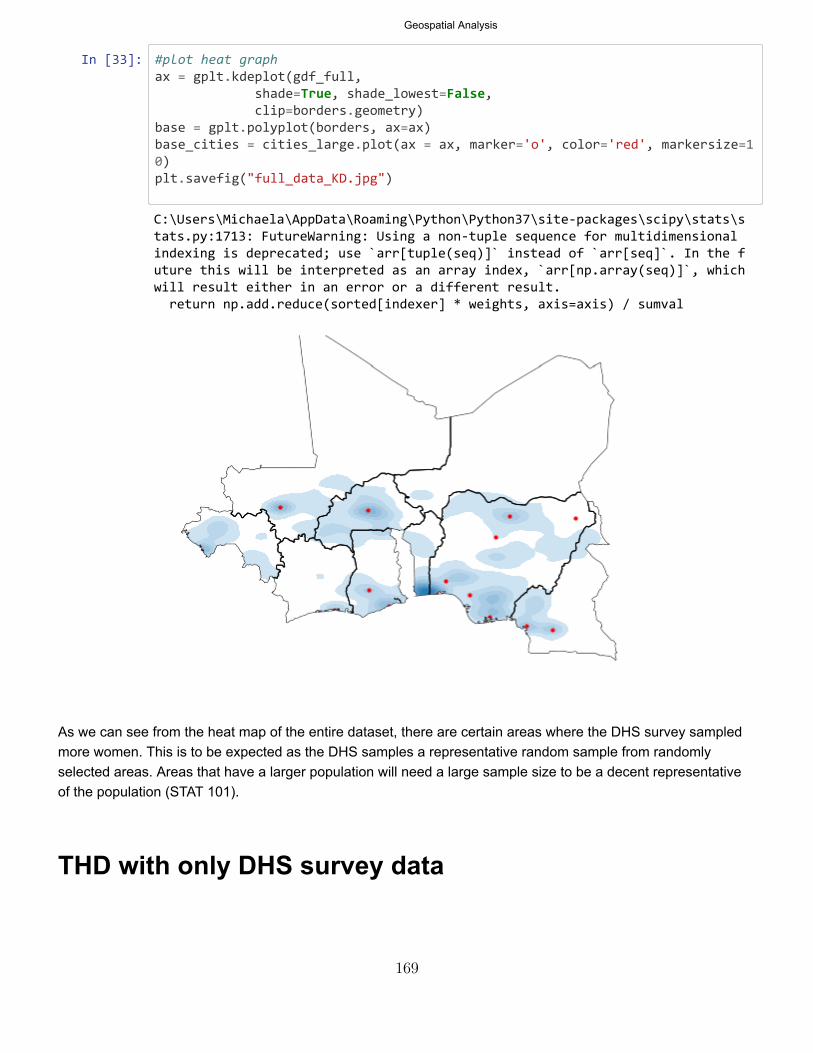
Geospatial Analysis

In [33]: #plot heat graph ax = gplt.kdeplot(gdf_full,


base = gplt.polyplot(borders, ax=ax) base_cities = cities_large.plot(ax = ax, marker='o', color='red', markersize=10) plt.savefig("full_data_KD.jpg")

As we can see from the heat map of the entire dataset, there are certain areas where the DHS survey sampledmore women. This is to be expected as the DHS samples a representative random sample from randomlyselected areas. Areas that have a larger population will need a large sample size to be a decent representativeof the population (STAT 101).

THD with only DHS survey data


169

Geospatial Analysis

In [34]: #THD2_24.0.1 - Higher instances of violence: points = gdfs1['gdf_24_0_1'] ax = gplt.kdeplot(points,


base = gplt.polyplot(borders, ax=ax) base_cities = cities_large.plot(ax=ax, marker='o', color='red', markersize=10)

print(points.shape) plt.savefig("THD_women_24_0_1.jpeg", bbox_inches='tight', pad_inches=0.1)


(12414, 448)

170

Geospatial Analysis

In [35]: #THD2_24.0.3 - Higher instances of violence: points = gdfs1['gdf_24_0_3'] ax = gplt.kdeplot(points,


base = gplt.polyplot(borders, ax=ax) base_cities = cities_large.plot(ax=ax, marker='o', color='red', markersize=10)

print(points.shape) plt.savefig("THD_women_24_0_3.jpeg", bbox_inches='tight', pad_inches=0.1)


(8468, 448)

171

Geospatial Analysis

In [36]: #2.0.1 - Mainly young and unmarried women - higher instances of violence ax = gplt.kdeplot(gdfs1['gdf_2_0_1'],

shade=True, shade_lowest=False, #n_levels = 50, clip=borders.geometry)

base = gplt.polyplot(borders, ax=ax) base_cities = cities_large.plot(ax = ax, marker='o', color='red', markersize=10)

plt.savefig("THD_women_2_0_1.jpg", bbox_inches='tight', pad_inches=0.1)

THD with DHS and ACLED Data

5.1.2 - 5.1.13 come out of the connected component who held 99% of remaining conflict instances after themajor split where data with 99% of the conflict went into one connected component and the rest was splitbetween singl and married women. I want to see what might be causing the split because it's hard to tell usingthe comparisions in Ayasdi.


172

Geospatial Analysis

In [38]: #THD2_5.1.2 - Frist break from 4.0.1 and only one to continue to decompose ax = gplt.kdeplot(gdfs2['gdf_5_1_2'],



plt.savefig("THD_all_5_1_2.jpg", bbox_inches='tight', pad_inches=0.1)


173

Geospatial Analysis

In [39]: #THD2_5.1.3 ax = gplt.kdeplot(gdfs2['gdf_5_1_3'],





174

Geospatial Analysis






175

Geospatial Analysis






176

Geospatial Analysis






177

Geospatial Analysis






178

Geospatial Analysis






179

Geospatial Analysis






180

Geospatial Analysis






181

Geospatial Analysis






182

Geospatial Analysis





^^ They seem to be more specific events.

These are the nodes after the major split


183

Geospatial Analysis

In [21]: #THD2_4.0.1 - Almost all instances of violence ax = gplt.kdeplot(gdfs2['gdf_4_0_1'],



#print(gdfs['gdf_4_0_1'].shape) print(gdfs2['gdf_4_0_1'].shape) plt.savefig("THD_all_4_0_1.jpg", bbox_inches='tight', pad_inches=0.1)


(96459, 448)

184

Geospatial Analysis

In [20]: #THD1_4.0.0 - married women with little conflict points = gdfs2['gdf_4_0_0'] print(points.shape) ax = gplt.kdeplot(points,


base = gplt.polyplot(borders, ax=ax) base_cities = gplt.pointplot(cities_large,ax=ax, color='red')

plt.savefig("THD_all_4_0_0.jpeg", bbox_inches='tight', pad_inches=0.1)

(111773, 448)


185

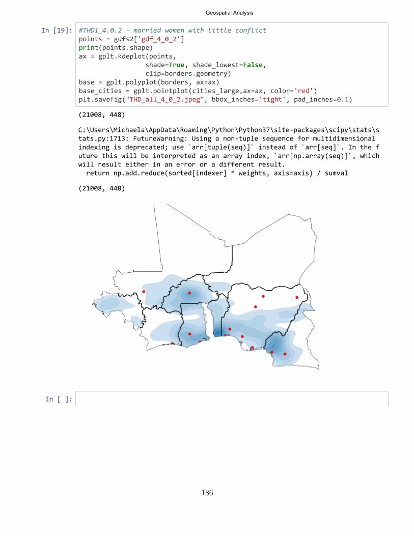
Geospatial Analysis

In [19]: #THD1_4.0.2 - married women with little conflict points = gdfs2['gdf_4_0_2'] print(points.shape) ax = gplt.kdeplot(points,


base = gplt.polyplot(borders, ax=ax) base_cities = gplt.pointplot(cities_large,ax=ax, color='red') plt.savefig("THD_all_4_0_2.jpeg", bbox_inches='tight', pad_inches=0.1)

In [ ]:

(21008, 448)


(21008, 448)

186

Bibliography

1. National Geographic’s Education Blog, “Africa’s Dazzling Diveristy,” 2015.https://blog.education.nationalgeographic.org/2015/02/18/

africas-dazzling-diversity/, [Accessed: 26- Feb- 2019].

2. J. Tesfu, “Mali Empire (ca. 1200- ),” 2008. https://www.blackpast.org/global-african-history/mali-empire-ca-1200/,[Accessed: 26- Feb- 2019].

3. Michigan State Univeristy: African Studies Center, “Module Seven (B),Activity Two: Colonial Exploration and Conquest in Africa,” in ExploringAfrica, World Press, 2018. http://exploringafrica.matrix.msu.edu/curriculum/unit-two/module-seven-b/, [Accessed: 26- Feb- 2019].

4. OECD, “Violent Events,” MAPS & FACTS: Sahal and West AFrica Club, 2015.

5. OECD, “Ebola killed more than 11,000 people,” MAPS & FACTS: Sahal andWest AFrica Club, Jan 2016.

6. OECD, “West African Girls are Being Married Off too Young,” MAPS &FACTS: Sahal and West AFrica Club, Mar 2016.

7. OECD, “Military Expenditures in West Africa,” MAPS & FACTS: Sahel andWest Africa Club, Jul 2018.

8. J. J. O’Connor and E. F. Robertson, “A History of Topology.” MacTutorHistory of Mathematics Archive, 1996.

9. R. Kraft, Illustrations of Data Analysis Using the Mapper Algorithm andPersistent Homology. Degree project, Kth Royal Institute of Technology: Schoolof Engineering Sciences, Stockholm, 2016.

10. G. Carlsson, “Three Properties of Topological Analysis,” 2014. https://www.ayasdi.com/blog/topology/three-properties-of-topological-analysis,[Accessed: 26- Feb- 2019].

11. A. Gilmore and Ayasdi, “The Shape of Data,” 2015.https://www.youtube.com/watch?v=zDe72aINF2s&t=491s,[Accessed: 26- Feb-2019].

12. F. Chazal and B. Michel, “An introduction to Topological Data Analysis:fundamental and practical aspects for data scientists,” arXiv e-prints,p. arXiv:1710.04019, 2017.

13. The Central Intelligence Agency (CIA), “The World Factbook,” 2018.

187

https://blog.education.nationalgeographic.org/2015/02/18/africas-dazzling-diversity/

https://blog.education.nationalgeographic.org/2015/02/18/africas-dazzling-diversity/

https://www.blackpast.org/global-african-history/mali-empire-ca-1200/

https://www.blackpast.org/global-african-history/mali-empire-ca-1200/

http://exploringafrica.matrix.msu.edu/curriculum/unit-two/module-seven-b/

http://exploringafrica.matrix.msu.edu/curriculum/unit-two/module-seven-b/

https://www.ayasdi.com/blog/topology/three-properties-of-topological-analysis

https://www.ayasdi.com/blog/topology/three-properties-of-topological-analysis

https://www.youtube.com/watch?v=zDe72aINF2s&t=491s

14. D. C. Conrad, Empires of Medieval West Africa. Chelsea House Publishers,2010.

15. A. Marc, N. Verjee, and S. Mogaka, The Challenge of Stability and Security inWest Africa. Washington, DC: Agence Francaise de Developpement/The WorldBank, 2015.

16. R. O. Collins, African History: Text and Readings, vol. 1. Princeton: MarkusWiener Publishers, 1990.

17. J. M. Kabia, Humanitarian Intervention and Conflict Resolution in WestAfrica: From ECOMOG to ECOML. Burlington, VT: Ashgate PublishingLimited, 2009.

18. I. W. Zartman, T. D. Bakary, A. A. Boahen, A. Gboyega, and D. Rothchild,Governance as Conflict Management: Politics and Violence in West Africa.Brookings Institution Press, dec 1996.

19. The World Bank, “World Bank Country and Lending Groups – CountryClassification,” 2018.https://datahelpdesk.worldbank.org/knowledgebase/articles/

906519-world-bank-country-and-lending-groups, [Accessed: 26- Feb-2019].

20. N. Bouchama, G. Ferrant, L. Fuiret, A. Meneses, and A. Thim, “GenderInequality in West African Social Institutions,” OECD: Sahal and West AfricaClub, no. 13, 2018.

21. International Crisis Group, “Nigeria : Women and the Boko HaramInsurgency,” tech. rep., International Crisis Group, dec 2016.

22. D. L. Heymann, L. Chen, K. Takemi, D. P. Fidler, J. W. Tappero, M. J.Thomas, T. A. Kenyon, T. R. Frieden, D. Yach, S. Nishtar, A. Kalache, P. L.Olliaro, P. Horby, E. Torreele, L. O. Gostin, M. Ndomondo-Sigonda,D. Carpenter, S. Rushton, L. Lillywhite, B. Devkota, K. Koser, R. Yates, R. S.Dhillon, and R. P. Rannan-Eliya, “Global Health Security: The Wider Lessonsfrom the West African Ebola Virus Disease Epidemic,” The Lancet, vol. 385,no. 9980, pp. 1884–1899, 2015.

23. R. Berglee, “Subsaharan Africa,” in World Regional Geography: People, Placesand Globalization, ch. 7, pp. 374–480, University of Minnesota LibrariesPublishing, 2012.

24. L. A. Mazzitelli, “Transnational Organized Crime in West Africa: theAdditional Challenge,” International Affairs, vol. 2006, no. April 2006,pp. 1071–1090, 2013.

188

https://datahelpdesk.worldbank.org/knowledgebase/articles/906519-world-bank-country-and-lending-groups

https://datahelpdesk.worldbank.org/knowledgebase/articles/906519-world-bank-country-and-lending-groups

25. B. Davidson, A History of West Africa 1000 - 1800. London: Addison-WesleyLongman Ltd, revised ed., Jul 1978.

26. N. Nunn and L. Wantchekon, “The Slave Trade and the Origins of Mistrust inAfrica,” American Economic Review, vol. 101, no. 7, pp. 3221–3252, 2011.

27. A. M. Duva, “The Lone Star: The Story of Liberia,” PBS, 2002.http://www.pbs.org/wgbh/globalconnections/liberia/essays/history/,[Accessed: 26- Feb- 2019].

28. N. Annan, “Violent Conflicts and Civil Strife in West Africa: Causes,Challenges and Prospects,” Stability: International Journal of Security &Development, vol. 3, no. 1, 2014.

29. P. Diaz, “The Empire in Africa,” 2006. Documentary: seehttps://www.imdb.com/title/tt0495103/, [Accessed: 26- Feb- 2019].

30. Vice, “The Cannibal Warlords of Liberia,” 2011.https://www.youtube.com/watch?v=ZRuSS0iiFyo&t=693s,[Accessed: 26-Feb- 2019].

31. CDC, “2014-2016 Ebola Outbreak in West Africa,” tech. rep., CDC, Dec 2017.

32. M. Mankad, Z. Ul-haq, L. Finnegan, F. Checchi, G. Graham, G. Alkema,P. Watt, and F. Goodwin, “A Wake-up Call: Lessons from Ebola for theWorld’s Health Systems,” tech. rep., Save the Children, 2015.

33. United Nations Development Programme, “Assessing the socio-economicimpacts of Ebola Virus Disease in Guinea, Liberia and Sierra Leone: The Roadto Recovery,” tech. rep., UNDP, 2014.

34. G. Ferrant and A. Kolev, “Does gender discrimination in social institutionsmatter for long-term growth? : Cross-country evidence,” OECD DevelopmentCentre Working Papers, pp. 1–45, 2016.

35. V. M. Hudson and H. Matfess, “In Plain Sight: The Neglected Linkage betweenBride Price and Violent Conflict,” International Security, vol. 42, pp. 7–40,2017.

36. N. D. Allen, “Assessing a Decade of U.S. Military Strategy in Africa,” Orbis,vol. 62, pp. 655–669, Aug 2018.

37. J. Borger, “US to send troops to Liberia,” The Gardian, 2003.https://www.theguardian.com/world/2003/jul/03/julianborger,[Accessed: 26- Feb- 2019].

189

http://www.pbs.org/wgbh/globalconnections/liberia/essays/history/

https://www.imdb.com/title/tt0495103/

https://www.youtube.com/watch?v=ZRuSS0iiFyo&t=693s

https://www.theguardian.com/world/2003/jul/03/julianborger

38. G. Myre, “The Military Doesn’t Advertise It, But U.S. Troops Are All OverAfrica,” npr, 2018.https://www.npr.org/sections/parallels/2018/04/28/605662771/

the-military-doesnt-advertise-it-but-u-s-troops-are-all-over-africa,[Accessed:26- Feb- 2019].

39. U.S. Africa Command Public Affairs, “U.S. Africa Command MissionStatement,” 2019. https://www.africom.mil/media-room/photo/31498/u-s-africa-command-mission-statement, [Accessed: 26- Feb- 2019].

40. United Nations Security Council (UNSC), “Resolution 2242,” 2015.

41. A. Gelman and J. Hill, “Missing-data imputation,” in Data Analysis usingRegression and Multilevel/Hierarchical Models (R. M. Alvarex, N. L. Beck, andL. L. Wu, eds.), ch. 25, pp. 529–545, New York, NY: Cambridge UniversityPress, 1st ed., 2007.

42. C. d. J. Oudraat and M. E. Brown, “Women, Gender, and Terrorism: TheMissing Links,” tech. rep., Women in International Security, Washington, DC,2016.

43. J. Krause, W. Krause, and P. Branfors, “Women’s Participation in PeaceNegotiations and the Durability of Peace,” International Interactions, vol. 44,no. 6, pp. 985–1016, 2018.

44. L. Woessmann, “The Economic Case for Education,” Education Economics,vol. 24, no. 1, pp. 3–32, 2016.

45. G. Psacharopoulos and H. A. Patrinos, “Returns to investment in education: adecennial review of the global literature,” Education Economics, vol. 26, no. 5,pp. 445–458, 2018.

46. Ayasdi, “Professor Gunnar Carlsson Intorduces Topological Data Analysis.”Youtube, 2013. https://www.youtube.com/watch?v=XfWibrh6stw, [Accessed:26- Feb- 2019].

47. G. Carlsson, “Topology and Data,” Bulletin of the American MathematicalSociety, vol. 46, no. 2, pp. 255–308, 2009.

48. J. R. Munkres, Topology. Prentice Hall, Inc., 2nd ed., 2000.

49. G. Singh, F. Memoli, and G. Carlsson, “Topological Methods for the Analysis ofHigh Dimensional Data Sets and 3D Object Recognition,” in EurographicsSymposium on Point-Based Graphics (M. Botsch, R. Pajarola, B. Chen, andM. Zwicker, eds.), pp. 1–11, The Eurographics Association, 2007.

50. A. Hatcher, Algebraic Topology. Cambridge: Cambridge University Press, 2002.

190

https://www.npr.org/sections/parallels/2018/04/28/605662771/the-military-doesnt-advertise-it-but-u-s-troops-are-all-over-africa

https://www.npr.org/sections/parallels/2018/04/28/605662771/the-military-doesnt-advertise-it-but-u-s-troops-are-all-over-africa

https://www.africom.mil/media-room/photo/31498/u-s-africa-command-mission-statement

https://www.africom.mil/media-room/photo/31498/u-s-africa-command-mission-statement

https://www.youtube.com/watch?v=XfWibrh6stw

51. K. Brown, D. Doran, R. Kramer, and B. Reynolds, “HELOC Applicant RiskPerformance Evaluation by Topological Hierarchical Decomposition,” CoRR,vol. abs/1811.1, pp. 1–10, 2018. https://arxiv.org/abs/1811.10658,[Accessed: 26- Feb- 2019].

52. A. Bak, “Stanford Seminar - Topological Data Analysis: How Ayasdi used TDAto Solve Complex Problems,” Nov 2013.https://www.youtube.com/watch?v=x3Hl85OBuc0&t=2930s,[Accessed: 26-Feb- 2019].

53. R. A. Fisher, “The Use of Multiple Measurements in Taxonomic Problems,”Annals of Eugenics, vol. 7, pp. 179–188, 1936.

54. D. Dheeru and E. Karra Taniskidou, “UCI Machine Learning Repository,”University of California, Irvine, School of Information and Computer Sciences,2017. http://archive.ics.uci.edu/ml, [Accessed 26- Feb- 2019].

55. M. Vicolau, A. J. Levine, and G. Carlsson, “Topology based data analysisidentifies a subgroup of breast cancers with a unique mutational profile andexcellent survival,” PNAS, vol. 108, pp. 7265–7270, Apr 2011.

56. L. Li, W.-y. Cheng, B. S. Glicksberg, O. Gottesman, R. Tamler, R. Chen, E. P.Bottinger, and J. T. Dudley, “Identification of Type 2 Diabetes Subgroupsthrough Topological Data Analysis of Patient Similarity — Ayasdi,” ScienceTranslational Medicine, vol. 7, pp. 1–16, Oct 2015.

57. Ayasdi, “Credit Card Fraud Detection & Modeling: Reduce overall fraudexposure by the analysis of complex transaction data,” tech. rep., Ayasdi, 2013.

58. T. Hastie, R. Tibshirani, and J. Friedman, “Random Forest,” in The Elementsof Statistical Learning: Data mining, Inference, and Prediction, Springer Seriesin Statistics, ch. 15, pp. 587– 603, Springer, New York, 2nd ed., 2009.

59. D. Xu, Y. Wang, Y. Meng, and Z. Zhang, “An Improved Data AnomalyDetection Method Based on Isolation Forest,” Proceedings - 2017 10thInternational Symposium on Computational Intelligence and Design, ISCID2017, vol. 2, pp. 287–291, 2017.

60. A. Beiden, “Ayasdi Support: t-SNE Lens?,” Jul 2017. https://ayasdicommunity.force.com/s/question/0D50P00003HCM2WSAX/tsne-lens,[Accessed: 26- Feb- 2019].

61. L. van der Maaten and G. Hinton, “Visualizing Data using t-SNE,” Journal ofMachine Learning Research, vol. 9, pp. 2579–2605, Nov 2008.

62. S. Arora, W. Hu, and P. K. Kothari, “An Analysis of the t-SNE Algorithm forData Visualization,” arXiv e-prints, pp. 1–32, Mar 2018.http://arxiv.org/abs/1803.01768, [Accessed: 26- Feb- 2019].

191

https://arxiv.org/abs/1811.10658

https://www.youtube.com/watch?v=x3Hl85OBuc0&t=2930s

http://archive.ics.uci.edu/ml

https://ayasdicommunity.force.com/s/question/0D50P00003HCM2WSAX/tsne-lens

https://ayasdicommunity.force.com/s/question/0D50P00003HCM2WSAX/tsne-lens

http://arxiv.org/abs/1803.01768

63. J. Lawhead, Learning Geospatial Analysis with Python. Packt Publishing,2nd ed., Dec 2015.

64. Ayasdi, “Knowledge: Selecting The Metric.” Blog, aug 2018. https://ayasdicommunity.force.com/s/article/Knowledge-Selecting-The-Metric,[Accessed: 26- Feb- 2019].

65. Python Software Foundation, “Python Language Reference, version 2.7,” 2001.https://www.python.org/download/releases/2.7/, [Accessed 26- Feb- 2019].

66. Python Software Foundation, “Python Language Reference, version 3.7,” 2008.https://www.python.org/downloads/release/python-370/, [Accessed: 26-Feb- 2019].

67. GeoPandas Development Team, “GeoPandas,” 2013.https://github.com/geopandas/geopandas, [Accessed: 26- Feb- 2019].

68. A. Bilogur, “Geoplot,” 2016. https://github.com/ResidentMario/geoplot,[Accessed: 26- Feb- 2019].

69. B. Sandvik, “World Borders Dataset,” 2009.http://thematicmapping.org/downloads/world_borders.php, [Accessed:26- Feb- 2019].

70. Eris, “World Cities,” Jun 2013. https://hub.arcgis.com/datasets/6996f03a1b364dbab4008d99380370ed_0,[Accessed: 26- Feb- 2019].

71. E. H. Boyle, M. King, and M. Sobek, “IPUMS-Demographic and HealthSurveys: Version 5 [West Africa - Women],” 2018.https://www.idhsdata.org/idhs/, [Accessed 26- Feb- 2019].

72. ICF, “The DHS Program Spatial Data Repository.”https://spatialdata.dhsprogram.com/home/, [Accessed: 26- Feb- 2019].

73. C. Raleigh, A. Linke, H. Hegre, and J. Karlsen, “Introducing ACLED ArmedConflict Location and Event Data,” Journal of Peace Research, vol. 47, no. 5,pp. 651–660, 2010.

74. T. D. Program, “Part I: Introduction to DHS Sampling Procedures,” Oct 2014.https://www.youtube.com/watch?v=DD5npelwh80, [Accessed: 26- Feb- 2019].

75. C. Raleigh and C. Dowd, “Armed Conflict Location and Event Data Project(ACLED) Codebook,” 2017. https://www.acleddata.com/wp-content/uploads/2017/01/ACLED_Codebook_2017.pdf, [Accessed: 26- Feb- 2019].

192

https://ayasdicommunity.force.com/s/article/Knowledge-Selecting-The-Metric

https://ayasdicommunity.force.com/s/article/Knowledge-Selecting-The-Metric

https://www.python.org/download/releases/2.7/

https://www.python.org/downloads/release/python-370/

https://github.com/geopandas/geopandas

https://github.com/ResidentMario/geoplot

http://thematicmapping.org/downloads/world_borders.php

https://hub.arcgis.com/datasets/6996f03a1b364dbab4008d99380370ed_0

https://hub.arcgis.com/datasets/6996f03a1b364dbab4008d99380370ed_0

https://www.idhsdata.org/idhs/

https://spatialdata.dhsprogram.com/home/

https://www.youtube.com/watch?v=DD5npelwh80

https://www.acleddata.com/wp-content/uploads/2017/01/ACLED_Codebook_2017.pdf

https://www.acleddata.com/wp-content/uploads/2017/01/ACLED_Codebook_2017.pdf

76. W. McKinney, “Data Structures for Statistical Computing in Python,” inProceedings of the 9th Python in Science Conference (S. van der Walt andJ. Millman, eds.), pp. 51–56, 2010.

77. F. Pedregosa, R. Weiss, and M. Brucher, “Scikit-learn: Machine Learning inPython,” Journal of Machine Learning Research, vol. 12, pp. 2825–2830, 2011.

78. O. Travis E, “A Guide to Numpy.” http://www.numpy.org/, [Accessed 26-Feb- 2019].

79. J. D. Hunter, “Matplotlib: A 2D Graphics Environment.”https://matplotlib.org/, [Accessed: 26- Feb- 2019].

80. S. Gillies and Others, “Shapely: manipulation and analysis of geometricobjects.” https://github.com/Toblerity/Shapely, [Accessed: 26- Feb- 2019].

81. M. Waskom, O. Botvinnik, D. O’Kane, P. Hobson, J. Ostblom, S. Lukauskas,D. C. Gemperline, T. Augspurger, Y. Halchenko, J. B. Cole, J. Warmenhoven,J. de Ruiter, C. Pye, S. Hoyer, J. Vanderplas, S. Villalba, G. Kunter,E. Quintero, P. Bachant, M. Martin, K. Meyer, A. Miles, Y. Ram, T. Brunner,T. Yarkoni, M. L. Williams, C. Evans, C. Fitzgerald, Brian, and A. Qalieh,“mwaskom/seaborn: v0.9.0,” Jul 2018.

193

http://www.numpy.org/

https://matplotlib.org/

https://github.com/Toblerity/Shapely

REPORT DOCUMENTATION PAGE Form ApprovedOMB No. 0704–0188

The public reporting burden for this collection of information is estimated to average 1 hour per response, including the time for reviewing instructions, searching existing data sources, gathering andmaintaining the data needed, and completing and reviewing the collection of information. Send comments regarding this burden estimate or any other aspect of this collection of information, includingsuggestions for reducing this burden to Department of Defense, Washington Headquarters Services, Directorate for Information Operations and Reports (0704–0188), 1215 Jefferson Davis Highway,Suite 1204, Arlington, VA 22202–4302. Respondents should be aware that notwithstanding any other provision of law, no person shall be subject to any penalty for failing to comply with a collectionof information if it does not display a currently valid OMB control number. PLEASE DO NOT RETURN YOUR FORM TO THE ABOVE ADDRESS.

1. REPORT DATE (DD–MM–YYYY) 2. REPORT TYPE 3. DATES COVERED (From — To)

4. TITLE AND SUBTITLE 5a. CONTRACT NUMBER

5b. GRANT NUMBER

5c. PROGRAM ELEMENT NUMBER

5d. PROJECT NUMBER

5e. TASK NUMBER

5f. WORK UNIT NUMBER

6. AUTHOR(S)

7. PERFORMING ORGANIZATION NAME(S) AND ADDRESS(ES) 8. PERFORMING ORGANIZATION REPORTNUMBER

9. SPONSORING / MONITORING AGENCY NAME(S) AND ADDRESS(ES) 10. SPONSOR/MONITOR’S ACRONYM(S)

11. SPONSOR/MONITOR’S REPORTNUMBER(S)

12. DISTRIBUTION / AVAILABILITY STATEMENT

13. SUPPLEMENTARY NOTES

14. ABSTRACT

15. SUBJECT TERMS

16. SECURITY CLASSIFICATION OF:

a. REPORT b. ABSTRACT c. THIS PAGE

17. LIMITATION OFABSTRACT

18. NUMBEROFPAGES

19a. NAME OF RESPONSIBLE PERSON

19b. TELEPHONE NUMBER (include area code)

Standard Form 298 (Rev. 8–98)Prescribed by ANSI Std. Z39.18

21-03-2019 Master’s Thesis OCT 2017 - MAR 2019

Women and Stability: A Topological View of the Relationship betweenWomen and Armed Conflict in West Africa

Pendergrass, Michaela, A. Ctr, The Perduco Group

Air Force Institute of TechnologyGraduate School of Engineering and Management (AFIT/EN)2950 Hobson WayWPAFB OH 45433-7765


United States Africa CommandCori FleserGender Advisor, J5HQ U.S. Africa CommandNIPR: [email protected]

USAFRICOM

DISTRIBUTION STATEMENT A:APPROVED FOR PUBLIC RELEASE; DISTRIBUTION UNLIMITED.

This work is declared a work of the U.S. Government and is not subject to copyright protection in the United States

The relationship between women and stability, if any, is a topic of much debate and research. Several large and influential organizationshave all researched women’s effect on stability. Furthermore, several of these world organizations, the United Nations, in particular, havedeclared gender equality to be a driving force in promoting stability and conflict prevention. Due to the United States active involvement inconflict prevention in such regions as West Africa, research concerning the relationship between women and stability is of particular interestthe United States Africa Command.As such, this research applied Topological Data Analysis, combined with other machine learning algorithms, to Demographic and HealthSurvey Program data combined with Armed Conflict Location and Event Data so as to observe the relationship between women’s statusand armed conflicts in the West African region. While this team did not observe any direct correlation between women’s well-being andstability - defined as a lack of armed conflict events - the chosen methodologies and data usage have potential implications for futureresearch concerning stability and conflict.

Economics, Women and Stability, West Africa, Topological Data Analysis, Geospatial Analysis

U U U UU 207

LTC C. M. Smith, Ph.D., AFIT/ENS

(937) 255-3636, x4318; [email protected]