Embed Size (px)
Citation preview

Women as Agents of Change:
Female Income, Social Affiliation and Household Decisions in South
India ∗
Nancy Luke† Kaivan Munshi‡
February 2005
Abstract
This paper provides empirical support for the view that women belonging to historically dis-advantaged communities, conveniently measured by caste in India, will emerge as active agentsof change when resources are made available to them, moving their families from the traditionaleconomy to the modern market economy. The setting for the study is the South Indian High Range,where female tea workers earn substantially more than male workers and economic conditions donot vary by caste. Controlling for total household income, we find that an exogenous increasein female income among the low castes significantly increases investments in schooling and moregenerally moves the family away from the home community. Female income effects, in contrast, areabsent among the high castes. These differences in the female income effect can explain, in part,the striking observation that educational attainment is higher among the low castes than the highcastes in the tea estates, reversing the usual pattern found elsewhere in India.
Keywords. Education. Marriage. Networks. Caste. Gender. Household decisions. Female income.JEL. D13. J12. J24. O12.
∗This project could not have been completed without the encouragement and support that we received from HomiKhusrokhan. We thank the management, staff, and workers of Tata Tea, Munnar, for their assistance and gracioushospitality during our extended stays in the tea estates. Binitha Thampi supervised the data collection and, togetherwith Leena Abraham, assisted us in the design of the survey. We are grateful to Suma Chitnis, Raquel Fernandez,Jonathan Gruber, Ignacio Palacios-Huerta, Padma Velaskar and especially Andrew Foster for many helpful discussions.Andrew Foster provided us with the numerical solution to the model and Chun-Fang Chiang, Alaka Holla, and JonathanStricks provided excellent research assistance. Sarah Williams and Naresh Kumar assisted us with the geo-mapping.Seminar participants at Brown, NYU, and the University of Washington provided useful comments. Research supportfrom the Mellon Foundation at the University of Pennsylvania, the Harry Frank Guggenheim Foundation, and NICHDgrant R01-HD046940 is gratefully acknowledged. We are responsible for any errors that may remain.
†Brown University‡Brown University and NBER

1 Introduction
Disparities in income and education persist across social groups in many developing countries such as
India even as economic globalization proceeds around the world. This paper explores the role that
women might play in reducing such disparities. We will argue that women belonging to historically
disadvantaged communities, conveniently measured by caste in India, might have a disproportionately
strong incentive to move themselves and their families from the traditional economy to the modern
market economy when resources are made available to them.
Hindu society was historically organized by caste into hereditary occupations, with the lower castes
relegated to menial and ritually polluting tasks. When new opportunities presented themselves un-
der British colonial rule the upper castes were quick to gain access to education and with it coveted
administrative and professional jobs, reinforcing existing disparities. Recognizing the historical in-
equities that have accompanied the caste system, the government of India has implemented policies
and programs to economically empower the lower castes since independence in 1947. Nevertheless,
a large caste-gap in wealth and educational attainment continues to persist in both urban and rural
India today. Our objective in this paper is to explore the role that low caste women might play in
closing this gap.
The setting for our analysis is the South Indian High Range, a mountainous area straddling the
modern Indian states of Kerala and Tamil Nadu. The High Range was virgin forest until it was
acquired by British planters and converted into tea plantations in the last quarter of the nineteenth
century. Since the plantation land was previously uninhabited, workers were brought to the High
Range from the plains in Tamil Nadu. Today, the workers on the tea plantations - or estates - are the
third-generation descendants of those migrants, whose population is supplemented by a fresh influx
of new workers from the “low country” in each subsequent generation through marriage.
The relatively isolated tea estates are well suited to the analysis we have in mind for two reasons.
First, in contrast with the pattern elsewhere in India, both men and women work on the tea estates.
Women work primarily as tea-leaf pluckers, whereas the men are employed in supporting tasks such
as weeding, spraying, and pruning, as well as in the estate tea factories. Women actually earn 15%
more than men on average, and these unusual wage patterns have now been in place for multiple
generations.
The second advantage of the setting we have chosen is that jobs are not assigned by caste in
1
the tea estates, in contrast once again with the patterns elsewhere in India. While the inequities
of the caste system are well known, a particularly egregious feature of this system specific to South
India was the institution of agrestic slavery, which committed the members of certain agricultural
labor sub-castes, or jatis, to a lifetime of servitude. The emancipation of slavery in India in the last
quarter of the nineteenth century coincided with the opening of the tea estates in the High Range,
and not surprisingly the bulk of plantation labor was made up of former slaves looking to improve
their opportunities. Due to their particularly disadvantaged historical circumstances, the former slave
castes continue to be distinct from all the castes above them in South Indian society and much of the
analysis in this paper will consequently classify them as “low castes,” including all the other castes in
the tea estates in the “high caste” category. What is remarkable about the plantation system is that
the former slaves, the lowest of the low castes, have the same jobs and access to the same housing,
educational, and medical facilities as the upper caste workers on the tea estates.
Most of the data used in the analysis are obtained from a survey of 3,700 female workers conducted
by the authors in 2003. These workers are employed by a single firm, the largest tea manufacturing
company in the world, that operates 23 plantations or “estates” in the High Range. Each estate
employs approximately one thousand workers and the sampled women were drawn randomly from all
23 estates. Annual incomes for all workers were also obtained over the 1997-2001 period from the
company’s computerized records to supplement the survey data.
Low and high caste workers have the same age and income in the tea estates. However, the low
caste workers have significantly higher schooling than the high caste workers, reversing the pattern
that we would expect to find elsewhere in the country. While educational attainment has increased
substantially over the past two generations, the same cross-caste patterns continue to be obtained
among the workers’ children as well.
The explanation for this striking observation that we put forward in this paper draws on the fact
that the workers continue to be tied to their ancestral communities in rural Tamil Nadu, despite
having lived in the tea estates for many generations. Loans and reciprocal transfers flow back and
forth between the tea estates and the origin communities, the children of the workers are often sent
home to study, and many workers will buy land, build a house, and return to their ancestral homes
when they retire. Perhaps the most distinctive feature of South Indian kinship structure is marriage
among close relatives (Karve 1953, Dumont 1986, Trautman 1981). These marriages traditionally
supported a primary social network at the level of the extended family, with overlapping primary
2

networks linking the endogamous sub-caste, or jati. Reinforcing existing network ties, many workers
continue to marry their children to relatives from the origin location in the traditional fashion.
A household in the tea estates can thus invest its scarce resources in an extended-family network
located in the ancestral home, with the expectation that it will receive a return on that investment
in the future. Alternatively, the household can invest in the nuclear family, particularly in children’s
education, with the expectation that the parents will be supported by their children in old-age. Given
the persistent caste differences in socioeconomic status outside the tea estates it seems reasonable to
assume that the low caste workers will have access to inferior networks back home in Tamil Nadu and
so will show a greater propensity to distance themselves from their home communities. The trade off
between the extended family and the nuclear family can thus explain, in part, the higher schooling
among the low castes in the tea estates as well as the accompanying observation that they are much
less likely to marry a relative or to end up living in the ancestral home.1
In this paper we are, however, particularly interested in the independent role that the low caste
women might have played in the shift from the extended family to the nuclear family. While both
men and women among the low castes face economic and social discrimination in rural Tamil Nadu,
we argue later that the low caste women will have a disproportionately strong incentive to distance
themselves and their children from the alcohol abuse and domestic violence that has historically
accompanied the poverty of the low castes, particularly the slave castes, in their ancestral locations.
Consistent with such a gender-gap in preferences among the low castes, we find that an exogenous
increase in low caste female income, net of total household income, weakens the family’s ties to the
home community as the woman gains bargaining power within the household.2 The children are
significantly less likely to marry a relative, they are less likely to be schooled in the ancestral location,
and they are less likely to ultimately settle there. At the same time, an exogenous increase in relative
female income increases the educational attainment of the low caste children, particularly the girls. In
contrast, we cannot reject the classical household income-pooling hypothesis for the high castes with
each of the outcomes just described. Low caste women independently influence important household1Along the same lines, Akresh (2004) shows in an interesting recent paper that network quality affects household
choices in Burkina Faso. The advantage of the research setting that we have chosen is that incomes do not vary by castein the tea estates, while the quality of the networks varies exogenously by caste, allowing us to more cleanly identify therole of community-based networks in shaping household decisions.
2We exploit two features of the production technology in the tea estates to construct statistical instruments for totalhousehold income and female income later in this paper. First, tea yields and, hence, male and female incomes varyexogenously with estate elevation. Second, income increases with experience, and hence the worker’s age, due to thepiece-rate wage contracts that are in place.
3
decisions in the tea estates and simple calculations reported later indicate that the role that these
women play in bringing about economic and social change, measured by education and marriage, is
quite substantial.
There is a large literature both in economics and sociology that seeks to understand how the
distribution of income within the household affects the allocation of resources (see Behrman 1997 and
Strauss and Thomas 1995 for exhaustive reviews). This literature is largely concerned with the choice
between private goods, which are enjoyed by a single individual, and public goods - notably children
- that benefit multiple individuals in the household. Consequently, much of the previous empirical
work has studied whether and how expenditures on different goods, particularly child education and
nutrition, vary with female income net of total household income. In contrast, we analyze how the
choice between investing in the extended family and the nuclear family is shaped by the distribution
of income within the household. This allows us to evaluate the effect of female income on major
decisions such as where to go to school and whom to marry, as well as on long-term outcomes such as
educational attainment and residential location.
In line with the results from the received literature, we find that an increase in female income
does lead to an increase in children’s schooling, particularly among the girls. But the additional
caste dimension that we incorporate in the analysis tells us that these effects vary by social group
and are concentrated among the low castes. These results, taken together, help explain the overall
differences in schooling by caste as well as the observation that schooling levels are extremely close
for the low caste boys and girls whereas a significant gender gap continues to persist among the high
caste children. Recent research from Bombay (Munshi and Rosenzweig 2003) shows that girls are
more receptive to new career opportunities, as measured by the schooling choices that are made for
them by their parents, than boys, who tend to be held back by the (male) caste-based labor market
networks that have historically operated in the city. In the tea estates we see once again that the
groups with the inferior (weaker) networks - in this setting, the low castes - are more receptive to
new opportunities, as demonstrated by their schooling and marriage choices. The analysis in Bombay
treats the household as the decisionmaking unit. In the tea estates, we find that low caste female
workers, who gain the most by moving their families from the traditional network-based economy to
the modern market economy, emerge as active agents of change when we look within the household.
The paper is organized in five sections. Section 2 describes the institutional setting, comparing
high and low castes in rural Tamil Nadu, as well as in the estates, separately by gender. A brief
4

history of the tea estates is also provided. Section 3 presents a simple model of household decision-
making that highlights the tradeoff between investing in the extended family and the nuclear family,
with implications for marriage and schooling decisions. The model also allows us to interpret the
female income effects and the total income effects that we obtain in the empirical analysis. Sec-
tion 4 presents the empirical results, beginning with simple caste-wise comparisons of schooling and
marriage among the workers’ children, by gender, and then proceeding to the regressions described
above. Additional support for the two major assumptions that underlie the empirical analysis, that
community-based networks in rural Tamil Nadu shape household decisions in the tea estates and that
the gender preference-gap varies by caste, is also provided in this section. Section 5 concludes.
2 The Institutional Setting
2.1 Caste and Gender in South India
Hindu society is divided hierarchically into four broad caste categories or varnas: Brahmins, Ksha-
triyas, Vaishyas, and Shudras. Within each varna are myriad endogamous sub-castes or jatis. And
arrayed below the four varnas, outside the caste system proper, are another host of untouchable jatis.
The slave castes occupied positions at the very bottom of this complex social system in South India.
Recognizing the historical inequities that accompanied the caste system and the persistence of many
of these inequities, the government of India has subsidized schooling, reserved seats in institutions of
higher education, and set aside a substantial fraction of government jobs for the low castes since
independence in 1947. The former untouchable castes, which include the slave castes, as well as some
Shudras who traditionally performed particularly abhorrent tasks are designated as Scheduled Castes
(SC’s) and deemed eligible for these government programs. Since caste has been officially abolished,
government statistics and large-scale data sets like the National Family Health Survey (NFHS) classify
individuals by their Scheduled Caste status alone. Thus, detailed jati-level data have been unavailable
from official sources since independence, complicating the comparison of outcomes in the tea estates
with outcomes in the workers’ ancestral homes in rural Tamil Nadu.
While all workers have access to the same opportunities and services in the tea estates, we expect
that conditions will vary by caste at home in rural Tamil Nadu. We consequently proceed to compare
Scheduled Castes (SC’s) with non-Scheduled Castes (non-SC’s) in Tamil Nadu, using the most recent
(1999) NFHS. Ideally, we would have liked to compare the slave castes with the castes above them,
5

but as noted, jati-level statistics are unavailable from standard data sources. The SC and non-SC
comparison nevertheless allows us to verify that the traditional caste hierarchy continues to determine
economic outcomes today.
The sampling frame for the NFHS is ever married women aged 15-49. Detailed information is
collected from each selected woman and her spouse (where relevant). Additional information on all
individuals residing in the house is collected in a separate household module. Comparing the SC
and non-SC husbands in rural Tamil Nadu in Table 1, Columns 1-2, there are no caste differences
by age, but schooling is significantly higher among the higher caste men. Employment levels are
extremely high in both caste groups, but non-SC men are much more likely to be employed in skilled
occupations. The NFHS does not report incomes, but these occupational differences indicate that
incomes will be greater in the higher castes. The same cross-caste patterns are obtained with the
urban sample in Columns 3-4, with high caste men having more schooling and being more likely
to be employed in skilled occupations than low caste men. Munshi and Rosenzweig (2003) report
qualitatively similar caste differentials in Bombay city as well, and we would in general expect this
pattern to be obtained throughout the country. The quality of a caste network in terms of its ability
to smooth risk, provide credit, and generate jobs will, in general, depend on the wealth of its members.
The preceding discussion suggests that high caste networks will be superior to low caste networks in
rural Tamil Nadu where the workers come from, as they are elsewhere in the country.
Comparing rural SC and non-SC women in Columns 5-6, both age and schooling do not vary
by caste. High caste women traditionally did not enter in the labor market, lowering their returns
to schooling and, by extension, their educational attainment. Consistent with this view, rural low
caste women are much more likely to be employed than rural high caste women, although they are less
likely to hold a skilled job conditional on being employed. Finally, caste comparisons among the urban
women in Columns 7-8 are very similar to those reported for the rural sample except that schooling
levels for the high caste women are now significantly higher than for the low castes and employment
levels for both caste groups are lower in the city than in the village.
2.2 A Brief History of the Tea Estates
The South Indian High Range was historically part of the state of Travancore; today it is situated
in the modern Indian state of Kerala (on the border with Tamil Nadu). Travancore was nominally
under the control of a native ruler, but under pressure from the local British Resident, the government
6

of Travancore began to grant “concession” land in perpetuity for the cultivation of coffee to British
planters from the 1860s onward.
After leaf disease destroyed the coffee crop in the 1870s, the planters experimented with a number
of crops before settling on tea. By the beginning of the twentieth century, the High Range had
developed into the most important tea producing area in Travancore. The shift from coffee to tea
led to fundamental changes in the operations of the plantations. Tea plantations require a stable
workforce, and while coffee could be simply left to dry in the sun, the tea leaves had to be processed in
a nearby factory before being transported. The original individual- or family-owned plantations were
consequently consolidated over time to take advantage of economies of scale. In 1890 James Finlay
and Company made an offer for a large share of the High Range concession, which was ultimately
accepted by the planters in 1897 after lengthy negotiations.
Since the concession land was previously uninhabited, labor had to be imported from elsewhere.
For reasons that are unclear to historians familiar with the area, it proved difficult to recruit labor
from Travancore itself (Kumar 1965, Baak 1997). Instead, the planters brought up workers from the
plains in the Madras Presidency (the modern Indian state of Tamil Nadu). As we noted earlier, a
large proportion of these workers belonged to the slave castes. Slavery in India differed from slavery
in other parts of the world in two important respects. First, the slaves in India could only be drawn
from specific castes. And, second, these slaves belonged to the same race and culture as their masters
and enjoyed certain rights, such as a customary wage (Kumar 1965, Alexander 1989). Nevertheless,
the slave castes remained the most wretched and downtrodden groups in South Indian society. For
example, Samuel Mateer, a Christian missionary writing in 1884 (cited in Kooiman 1989: 18), describes
how the slaves were “bought and sold like cattle, flogged like buffaloes, made to work all day for a little
rice, and kept at a distance as polluted ... suffering from ignorance and evil habits of drunkenness and
vice.”
The British noted the existence of slavery as soon as they arrived in South India at the beginning
of the nineteenth century, but they did little to change the system initially except to protect the
slaves from its worst abuses (Kumar 1965). It was only with the passing of the Penal Code in 1861
that a man could actually face legal prosecution if found in the possession of a slave, finally freeing
the slave castes (Hjejle 1967). The emancipation of the slaves coincided with the opening up of the
plantations in the High Range, and not surprisingly a large proportion of the labor force was recruited
from the (former) slave castes, who were looking to improve their economic opportunities. At the
7

same time, upper caste workers are well represented in the tea estates. Using census data, Kumar
(1965) documents that the population of the Madras Presidency, the major source region for labor in
the tea estates, rose by 300 percent between 1802 and 1901. This population increase, together with
the structural change in the economy brought about by colonialism, displaced many individuals from
their traditional caste occupations, inducing them to migrate to the tea estates as agricultural labor.
Initially the planters sent their own agents to recruit workers from the plains. But within a short
time the workers began to migrate on their own, in gangs drawn from the same jati, and led by
a kangany, or foreman. The kangany was responsible for transporting his gang to the High Range
(a dangerous and arduous journey), negotiating wages and other employment conditions there, and
eventually supervising his workers (Kumar 1965). The size of the workforce fluctuated with the
tea crop in the early years, and workers were recruited on fixed term contracts usually running for
nine months (Baak 1997). The problem with the short-term contracts was that the workers would
often return to the plains without advanced notice or be easily induced to switch companies at a
slightly higher wage. The Criminal Breach of Contract Act, introduced in 1865 by the Travancore
government, helped reduced this problem for a while. But the planters were forced to switch to a
permanent workforce with the abolition of the Act in the 1930s. With all the unpredictable movement
back and forth between the High Range and Tamil Nadu, it is unlikely that the workers were sorted
systematically across Finlay estates by ability when permanent employment status was first granted.
Permanent workers and their families were provided free housing in “labor lines” located on each
estate. To ensure that at least some of the children of the workers would be employed in the future,
company rules prevented workers from shifting across estates, or new workers from entering the estates,
except through marriage. James Finlay and Company gradually sold all its properties to a wholly
Indian-owned company, Tata Tea, over the course of the 1970s and 1980s, and the divestment process
was completed in 1986. Tata Tea has continued to keep the rules restricting worker mobility in
place. The workers on the tea estates are the third generation descendants of the workers who were
hired permanently in the 1930s, supplemented by the influx of fresh migrants in each generation
that followed through marriage. This stability in economic opportunities and access to health and
education facilities, over the worker’s lifetime and across multiple generations, no doubt played an
important role in the shift away from the home networks that we document below.
8
2.3 Caste and Gender in the Tea Estates
This paper uses data collected by the authors in two phases in 2002-2003. Annual incomes for all
workers over the 1997-2001 period were obtained from the company’s computerized records on an
initial trip to the tea estates in February-March 2002. Historical climate data from 1965 to 2001 and
the elevation of each estate were also collected on this visit. Subsequently, we conducted a survey of
4,000 female workers on a second visit, from December 2002 to March 2003.
Each estate office maintains a “family card” listing the individuals residing in each unit in the
labor lines and their relationship to the (typically male) household head. The information on the
family cards was collected and entered on computer on our first visit to the tea estates in 2002,
and the sampling frame for the subsequent survey in 2002-2003 was restricted to wives of (male)
household heads. The sampling frame ultimately comprised 11,700 women from which 4,600 were
drawn randomly and interviewed at their homes.
Since the list of workers was one year old at the time of the survey, some of the workers in the
sample had left employment by February 2003. Other workers were not at home on the day of the
interview and the revisit date. The 4,600 selected workers reside in 86 divisions in the 23 estates
spread all over the area (some of the estates are as far as 25 km from Munnar, the only town in the
area, where the survey team was based). Female workers pluck tea from 8AM until 5PM on weekdays,
so they could only be interviewed in the late evenings and on weekends. These logistical difficulties
forced us to schedule only one call-back for missed interviews. Nevertheless, 3,994 schedules were
ultimately completed, leaving us with an overall response rate of 89.1%.
Each worker is assigned a permanent identity number by the company, which we used to merge
the survey data with the individual incomes collected earlier from the company’s records. Discarding
mismatches between the identity numbers recorded in the survey and the administrative records, as
well as mismatches between the identity numbers in the survey and the family card, we were left with
3,700 couples in which the woman was the wife of a household head and for whom we had income
information for both spouses. The survey instrument collected detailed information on the background
of the respondent, her husband, and their parents. We also collected information on the respondent’s
children and their spouses (where relevant), paying particular attention to the marriage and schooling
choices that were made by the workers for their children.
Table 2 compares characteristics of the workers, separately for males and females, by caste. As
9

noted, the majority of the initial migrants to the tea estates belonged to the slave castes and two-thirds
of the workers today are drawn from those castes. The slaves went by different names in different
parts of South India; in the Tamil-speaking areas there were two slave jatis, known as the Pallars
and the Paraiyars, who together accounted for somewhere between 10 and 20 percent of the total
population in the nineteenth century (Kumar 1965).3 The slave castes faced particularly adverse
conditions historically, and the emancipation of slavery by the British and the subsequent abolition
of the caste system by the Indian government appear to have done little to change the economic and
social circumstances of these lowest of the low castes in rural Tamil Nadu. Kapadia’s study (1995) set
in one rural Tamil village, for example, describes how “the Pallars, Christian Paraiyars, and Wottans
(Hindu Paraiyars) in Aruloor all continue to be regarded as ‘untouchables,’ as they have been for
centuries” (p. 9). The analysis that follows will consequently restrict the low castes to the Pallars and
the Paraiyars, collecting all other jatis in the estates in the high caste category.4
Low caste and high caste workers, both males and females, have the same age and income in
Table 2, Panel A. In contrast, the low caste workers have significantly higher schooling than the upper
caste workers, for both men and women, reversing the patterns from rural and urban Tamil Nadu
reported in Table 1. Our explanation for the unusual schooling patterns in the tea estates relies on
differences in the quality of home networks and, by extension, differences in the level of attachment
to these networks by caste. Here the institution most responsible for keeping ties with the home
community in place over multiple generations is the marriage institution. Marriage in South India
traditionally occurred among relatives, with overlapping extended-family networks linking the entire
jati.5 Kapadia’s (1995: 19) ethnographic research in a Tamil village describes how “marriageable kin
(kalyana murai) were more important in everyday life than lineage kin (pankali). The simple fact
was that one got more from them [affines] than from patrilineal [lineage] kin, and for this reason
one was more involved with them.” Those workers in the estates that followed traditional marriage3Pallar is derived from pallam, the Tamil word for lowness and Paraiyar means outcaste (hence the English “pariah”).4In a previous version of the paper (Luke and Munshi 2004) we showed that the other Scheduled Castes in the tea
estates were actually closer to the forward (non-Scheduled) castes than to the former slaves in terms of their schoolingand marriage behavior, emphasizing the diversity that exists within the Scheduled Castes. All the results that followwould go through with the alternative SC classification in any case, since the Pallars and the Paraiyars account for thebulk of the Scheduled Castes in the tea estates.
5The term “cross-cousin marriage” is sometimes used to describe marriage patterns in the South Indian kinshipsystem. This is somewhat of a misnomer since traditionally the most preferred matches for a woman were the mother’sbrother, the mother’s brother’s son, and the father’s sister’s son. Among our female respondents who married a relative,12.5% married the mother’s brother, 25.4% married the mother’s brother’s son, and 22.3% married the father’s sister’sson. The remaining 39.8% married some other relative.
10

patterns typically found related spouses who grew up in the origin location for their children. But
marriage patterns respond to changes in the economy. Traditional cross-cousin marriage, for example,
has declined all over South India in recent decades, with relatively wealthy and educated individuals
exiting the network to match on the “open” marriage market (Kapadia 1995). If the low castes in the
tea estates are indeed distancing themselves from their rural networks and investing instead in their
children’s human capital then we should expect them to show the greatest propensity to deviate from
the traditional marriage patterns as well.
Table 2, Panel B compares marriage patterns by caste in the tea estates. To begin with, we
see that both low caste and high caste workers adhere to the fundamental social rule of marriage
within the jati. The low castes actually have slightly lower levels of out-marriage, perhaps due to the
continuing stigma associated with marriage into the former slave castes. However, consistent with the
preceding discussion, the low caste workers are much less likely to marry a relative. It then follows
mechanically that the high caste workers will be more likely to be first generation arrivals in the tea
estates. Households that distance themselves from the home community invest less in the extended
family network over their working lives and, not surprisingly, the parents of the low caste workers are
much less likely to have retired in the home location.
We close this section by discussing alternative explanations for the caste-gap in schooling and
marriage observed in Table 2. Low caste jatis are larger on average than high caste jatis in the
tea estates as a consequence of historical settlement patterns. Since the social rule of endogamous
marriage within the jati continues to be adhered to, low caste workers will have more eligible partners
who do not belong to their primary extended family network to choose from within the tea estates.
Differences in the local marriage market might then explain differences in marriage patterns and, by
extension, schooling choice across castes. While there are only two low caste jatis, there is sufficient
size variation across the more numerous high caste jatis to test whether size affects schooling and
marriage within that broad caste group. Controlling for the age of the man and the woman, we find
that jati size has no effect on these outcomes (not shown).
A second concern is that if workers systematically selected into the tea estates, and these historical
selection pressures varied by caste, then low caste and high caste workers would differ on dimensions
other than network quality, such as individual ability.6 One simple test of such ability differences6If we allowed for heterogeneous extended family networks within broad caste groups then we would expect high
castes with relatively poor networks to have migrated to the tea estates. But this would, if anything, reduce networkquality differences between low and high castes, providing us with a lower bound on the caste effects that we attempt to
11

would be to compare incomes in the tea estates by caste. We have already seen that these incomes do
not vary by caste, for both men and women, but other attributes, such as initiative and responsiveness
to new opportunities, which are not reflected in estate incomes, might nevertheless determine schooling
and marriage choices.
Table 3 explores how closely the households in the tea estates adhere to traditional norms of
behavior, which might be indicative of how responsive they will be in general to new opportunities.
Low caste women have traditionally worked outside the home and we saw in Table 1 that they continue
to be more likely to enter the labor force than high caste women, both in rural and in urban Tamil
Nadu. The income that this work generated has given them some control of the household budget and
some influence in household decision-making. High caste women, in contrast, were accorded greater
status within the household and in the broader community, at the cost of substantial restrictions on
their mobility and autonomy (Geeta 2002, Kapadia 1995, Chakravarti 1993).
Autonomy - the ability to make independent choices and the power to influence household decisions
- is generally extremely difficult to measure. The questions on female autonomy in our survey focussed
on the ability of women to make consumption choices without permission from their husbands. High
caste female workers are significantly more likely to report that they can buy a sari or jewelry and
that they can remit money to their parents without spousal permission than low caste women in Table
3, Panel A. There is doubtless a social aspect to female autonomy and we could imagine that caste
differences in female autonomy at home in rural Tamil Nadu would have persisted in the tea estates.
But if they did, they disappeared at least a generation ago; the caste patterns observed for the female
workers in Table 3 are obtained for their mothers as well.
Another aspect of decision-making that can be observed in principle is control of the budget. Men
have historically collected wages for their wives and themselves in the tea estates, and the statistics
reported in Table 3 suggest that this practice continues. Notice, however, that high caste women are
significantly more likely to collect their own salaries than low caste women. This caste difference is
obtained with the full sample of households and a restricted sample in which both the husband and
the wife work on the estates. Nominal control of a share of the budget does not necessarily translate
into real control of household resources, but there is no indication from any of the statistics in Table
3 that high caste women have less autonomy than low caste women.
Table 3, Panel B compares housework by caste. The respondents were asked how frequently their
identify in this paper.
12

husbands helped with a variety of traditionally female household tasks, including cooking, cleaning,
and child-care. We see no differences by caste, in contrast once again with what we would expect
to find elsewhere in Tamil Nadu. The high caste workers appear to be at least as progressive as the
low caste workers for all the measures that we report in Table 3. It is only with a particular set of
household choices, notably education and marriage, that the high castes lag behind the low castes,
leading us to conclude that it is variation in the quality of the home networks rather than individual
heterogeneity that is responsible for this caste-gap. Later in Section 4 we will provide independent
support for the view that networks are shaping household decisions in the tea estates.
3 Household Decisions in a Network-Based Economy
3.1 Timing of Decisions and Returns to Investment
Each individual lives for three periods in the simple overlapping generations model that we present
in this section. The individual is sent to school in the first period; we ignore the temporal aspect of
schooling and assume that educational attainment is determined in the first period itself and depends
on the resources that the parents allocate to schooling. The individual works during the second period
of his life, receiving his income in advance at the beginning of that period. The individual’s parents
arrange his marriage at the beginning of the second period as well, at which time a child is born.
The individual and his spouse use the incomes that they receive at the beginning of the second
period of their lives to invest in their network in the ancestral location, invest in their child’s schooling,
and to send transfers to their parents. They will subsequently choose a marriage partner for their child
at the beginning of the third and final period of their lives, in which they will live off the returns to
the investments in the extended family and the nuclear family that they made in the previous period.
Notice that the model ignores individual ability, which could determine parental incomes as well as
the choices that are made for the children. Unobserved ability will, however, play an important role
in the discussion on identification that follows in Section 4.2.
The returns to the investments that the parents make will depend on the quality of their home
networks, which varies by caste, as well as on the marriage choice that they make for their child.
Marriage to close relatives in the South Indian kinship system strengthens existing network ties instead
of building new ones, as in North India. South Indian kin networks have thus been seen to be more
cohesive, albeit restricted in geographic and social range, than their North Indian counterparts (Karve
13
1953, Dumont 1986, Trautman 1981). One way in which workers far away in the tea estates can
compensate for the geographical separation from their community is to marry their child into the
network. Such alliances reduce social distance and lower the probability that members of the network
far away in the origin location will renege on their obligations to the parents in the future. The model
thus assumes that the returns to investing in the extended family are higher when the parents marry
their child to a relative, within any caste.
In contrast, we expect that the returns to investment in the child’s schooling will decline with
marriage into the network within any caste. Such marriages increase the probability that the child will
end up living and working in the ancestral location in rural Tamil Nadu where the returns to schooling
are relatively low. Moreover, individuals that marry on the “open” market match on attributes such as
education and wealth. Thus, individuals that marry into the network, where matches are determined
by kinship rather than by individual attributes, forego the additional returns to schooling that they
would obtain through the marriage market.
How do the returns to investment in the extended family network and the nuclear family vary
by caste? The low castes were historically relegated to low-paying, menial occupations, and the
persistence of these economic disparities has been noted earlier in the paper. The quality of a network
will depend to a large extent on the resources of its members, so we would expect the quality of the low
caste networks to be relatively poor in this case. This implies, in turn, that the returns to investment
in the network will be lower among the low castes than the high castes.
It is less easy to predict how the returns to schooling vary by caste. Educated children could find
jobs in the city, where the returns to schooling are largely independent of caste.7 But those children
that marry into the network could end up living in the ancestral location and working in the traditional
caste occupation, in which case the returns to schooling could vary by caste. Schooling is in general a
way to escape the network and the traditional caste occupation. The caste differences in the returns
to schooling that we have described are consequently likely to be small, relative to the corresponding
caste differences in the returns to investment in the extended family network. The model that follows
will assume, for simplicity, that returns to schooling do not vary by caste. Castes will be distinguished
by the returns to investment in the network alone.7Munshi and Rosenzweig (2003) describe how caste-based networks operate in the city as well. But these networks
tend to be active in jatis that are well established in particular urban centers. None of the jatis in our sample haveestablished such a presence in Indian cities.
14
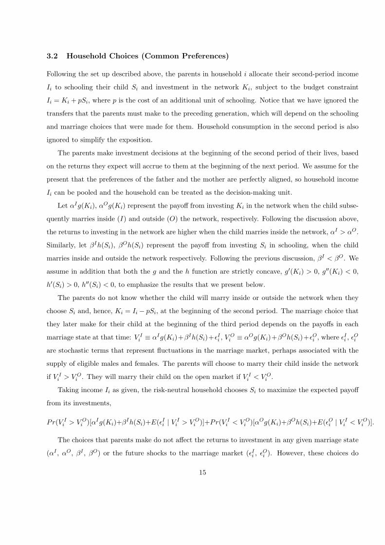
3.2 Household Choices (Common Preferences)
Following the set up described above, the parents in household i allocate their second-period income
Ii to schooling their child Si and investment in the network Ki, subject to the budget constraint
Ii = Ki + pSi, where p is the cost of an additional unit of schooling. Notice that we have ignored the
transfers that the parents must make to the preceding generation, which will depend on the schooling
and marriage choices that were made for them. Household consumption in the second period is also
ignored to simplify the exposition.
The parents make investment decisions at the beginning of the second period of their lives, based
on the returns they expect will accrue to them at the beginning of the next period. We assume for the
present that the preferences of the father and the mother are perfectly aligned, so household income
Ii can be pooled and the household can be treated as the decision-making unit.
Let αIg(Ki), αOg(Ki) represent the payoff from investing Ki in the network when the child subse-
quently marries inside (I) and outside (O) the network, respectively. Following the discussion above,
the returns to investing in the network are higher when the child marries inside the network, αI > αO.
Similarly, let βIh(Si), βOh(Si) represent the payoff from investing Si in schooling, when the child
marries inside and outside the network respectively. Following the previous discussion, βI < βO. We
assume in addition that both the g and the h function are strictly concave, g′(Ki) > 0, g′′(Ki) < 0,
h′(Si) > 0, h′′(Si) < 0, to emphasize the results that we present below.
The parents do not know whether the child will marry inside or outside the network when they
choose Si and, hence, Ki = Ii − pSi, at the beginning of the second period. The marriage choice that
they later make for their child at the beginning of the third period depends on the payoffs in each
marriage state at that time: V Ii ≡ αIg(Ki)+βIh(Si)+εI
i , V Oi ≡ αOg(Ki)+βOh(Si)+εO
i , where εIi , εO
i
are stochastic terms that represent fluctuations in the marriage market, perhaps associated with the
supply of eligible males and females. The parents will choose to marry their child inside the network
if V Ii > V O
i . They will marry their child on the open market if V Ii < V O
i .
Taking income Ii as given, the risk-neutral household chooses Si to maximize the expected payoff
from its investments,
Pr(V Ii > V O
i )[αIg(Ki)+βIh(Si)+E(εIi | V I
i > V Oi )]+Pr(V I
i < V Oi )[αOg(Ki)+βOh(Si)+E(εO
i | V Ii < V O
i )].
The choices that parents make do not affect the returns to investment in any given marriage state
(αI , αO, βI , βO) or the future shocks to the marriage market (εIi , εO
i ). However, these choices do
15

affect the marriage state that the child ends up in, which will in turn determine the family’s expected
payoff. This feature of the choice problem distinguishes our model from the standard household
budget allocation problem, generating some non-standard predictions that are specific to economic
environments in which networks are active.
The expression for the household’s expected payoff, described above, can be simplified as,
F (∆V )[∆V + ξIi (∆V ) − ξO
i (∆V )] + [ξOi (∆V ) + αOg(Ki) + βOh(Si)]
where ∆V ≡ ∆αg(Ki)+∆βh(Si) measures the additional deterministic return from marrying inside
the network, and F characterizes the distribution of εOi − εI
i . ∆α ≡ αI − αO > 0, ∆β ≡ βI − βO < 0.
Notice that F (∆V ) ≡ Pr(V Ii > V O
i ), ξIi (∆V ) ≡ E(εI
i | V Ii > V O
i ), ξOi (∆V ) ≡ E(εO
i | V Ii < V O
i ), can
all be expressed as functions of ∆V .
The second term in square brackets in the expression above represents the expected payoff when the
child marries outside the network. The first term in square brackets reflects the additional (expected)
payoff when the child marries inside the network, which could be negative. Changes in Si affect
the expected payoff when the child marries outside, the additional expected payoff when the child
marries inside, as well as the probability that the child will end up marrying inside, F (∆V ). All the
terms which are functions of ∆V in the expression above distinguish our problem from the standard
household budget allocation decision in which there is only a single state of the world. Collecting all
these terms, W (∆V ) ≡ F (∆V )[∆V + ξIi (∆V ) − ξO
i (∆V )] + ξOi (∆V ), the expression for the expected
payoff can be simplified even further as,
W (∆V ) + αOg(Ki) + βOh(Si).
Maximizing the expected payoff with respect to Si, the first order condition is obtained as
∂W
∂Si+ βOh′(Si) − αOpg′(Ki) = 0. (1)
Assuming that an interior solution to the household’s choice problem is obtained, how do these
choices vary by caste? ∆α, which measures the decline in the returns to investment in the network
when the child marries outside the network, will depend in general on cohesiveness within the caste
and, hence, the propensity of network members to renege on their obligations. While we do expect
that the returns to investment in the network to be lower among the low castes in both marriage
16

states, we have no prior belief about the cohesiveness of these castes. Thus, we assume that ∆α does
not vary by caste, but that αI , αO are both lower in the low castes. Moreover, we noted earlier that
the returns to schooling should be comparable across castes when the children marry inside or outside
the network. This implies that ∆β, βO do not vary by caste.
To derive comparative statics with respect to αO, it is convenient to assume that there is a
continuum of castes indexed by the parameter αO, which is increasing in network quality, and then
implicitly differentiate the first order condition to obtain
dSi
dαO=
pg′(Ki)SOC
.
Since SOC < 0 by assumption, dSi/dαO < 0. Incomes do not vary by caste in the tea estates,
and so the comparative statics derived above imply that the low castes, with lower αO than the high
castes, will invest more in schooling and less in the network than the high castes. What does this tell
us, in turn, about marriage patterns by caste?
d∆V
dαO= [∆βh′(Si) − ∆α · pg′(Ki)]
dSi
dαO> 0
since dSi/dαO < 0. The probability of marrying inside the network F (∆V ) is increasing in ∆V ,
which implies that the low castes, with low αO and hence low ∆V , should be less likely to marry
within their networks. The assumption that low caste workers have access to inferior home networks,
together with the equality of incomes in the tea estates, thus provides one explanation for the caste
differences in schooling and marriage among the workers that we noted in Table 2.
3.3 Household Choices (Gender-specific Preferences)
The high castes will have higher schooling than the low castes in rural Tamil Nadu and under normal
circumstances with movement back and forth between the ancestral homes and the tea estates we
would expect these caste patterns to have been retained among the workers as well. The preceding
discussion suggests, however, that the usual pattern could actually be reversed if the difference in
network quality across castes is sufficiently large. The analysis that follows explores the additional
role that low caste women might have played in changing schooling and marriage patterns in the tea
estates, based once again on underlying differences in the caste networks.
When male and female preferences differ within the household, models of collective decision-making
predict that a relative increase in female income will shift household choices along the Pareto frontier to
17

a point that the woman prefers. This result is obtained regardless of whether additional restrictions are
placed on the cooperative equilibrium as in Manser and Brown (1980), McElroy and Horney (1981),
and Lundberg and Pollak (1993), or whether only Pareto optimality is assumed as in Chiappori
(1992) and Browning et al. (1994). To identify an independent role for low caste women in influencing
household decision-making, we consequently look within each caste to estimate regressions of the form
yi = γFIi + λIi + Xiη + εi, (2)
where yi is the choice that household i makes for its child, Ii is total income in the household, FIi
is female income, Xi is a vector of control variables, and εi collects all the unobserved determinants
of the household’s choice. The γ coefficient will be significantly different from zero when the woman
independently influences decisions within the household.8 Outcomes of interest yi include schooling
attainment, which will depend on investments in schooling Si, as well as the probability that the child
will marry into the network F (∆V ).
We begin by deriving predictions for the λ coefficient in equation (2). The regressions will be
estimated separately by caste, and so we assume that αO, βO, ∆α, ∆β are constant across households
and then proceed to derive comparative statics with respect to Ii: dSi/dIi and dF (∆V )/dIi. Starting
with the effect of household income on the child’s schooling, the usual result is that an increase in
income should increase investment in schooling (S) and the network (K), since both the g and the
h functions are strictly concave. The complication that arises in this framework is that an increase
in income, by changing S and K, will change the probability that the child will be married into the
network. If this probability increases sufficiently, with its associated decline in the returns to schooling,
then the net effect on schooling could actually be negative. The assumed concavity in the g and h
functions implies that the returns to S and K will be declining at the margin in any given marriage
state. But the effect of a change in S (and K) on the probability of marrying inside the network is not
necessarily declining in this manner, and so the additional complication that arises is that a corner
solution could in principle be obtained.
To illustrate the possibility that an increase in household income could lead to a decline in schooling
when networks are active we solved the model numerically in a previous version of the paper (Luke8We could, in principle, include any measure of the income distribution or the income of any individual to test
the hypothesis that income is pooled within the household. The specification that we have chosen allows us to easilydetermine the direction in which the women shift household decisions.
18

and Munshi 2004), assuming that εIi , εO
i were characterized by the extreme value distribution and
suitably parameterizing the g(Ki) and h(Si) functions to ensure that an interior solution (SOC < 0)
was always obtained.9 The sign of dSi/dIi was seen to vary with the parameter values that were
chosen, consistent with the discussion above.
The regressions that we will later report show that dSi/dIi < 0 for both castes. The preceding
discussion indicated that an increase in the probability of marrying into the network with income
dF (∆V )/dIi > 0 was a necessary condition to obtain this result. To verify that this is indeed the
case, we proceed to show that dSi/dIi < 0 implies dF (∆V )/dIi > 0. Differentiating ∆V with respect
to Ii,
d∆V
dIi= ∆αg′(Ki) +
∂∆V
∂Si
dSi
dIi.
Since ∂∆V/∂Si = ∆βh′(Si)−∆α · pg′(Ki) < 0 and F (∆V ) is increasing in ∆V , the result follows
directly from the expression above. The negative effect of household income on schooling that we
later obtain is explained by the fact that an increase in income ties the household more closely to
its network in this economy, lowering the returns to children’s schooling, and we will verify that an
increase in household income indeed increases the probability that the children will marry within the
network.
This last result is very likely to be a consequence of the special economic circumstances in the tea
estates. In most other settings we would expect high income (or high ability) individuals to show the
greatest propensity to distance themselves from the network, to avoid subsidizing the other members,
and this is what we have found in our own previous research in Kenya (Luke and Munshi 2003) and
India (Munshi and Rosenzweig 2003). The richer households in this setting might, however, be able to
avoid many of their social obligations due to their geographical separation from their home locations
and the relative isolation of the tea estates, and we will return to this point below.
Next, consider the γ coefficient in equation (2); conditional on household income Ii, what effect
does female income FIi have on household decisions? An independent female income effect will only be
obtained if male and female preferences differ and we will argue below that the gender preference-gap
is likely to be most severe among the low castes.
Poverty is often associated with negative outcomes such as male alcohol abuse and domestic vio-
lence that must be borne disproportionately by women. For example, high levels of alcohol consump-9g(Ki), h(Si) were specified to be quadratic functions of Ki and Si respectively. The advantage of the extreme value
distribution is that the first order condition has a simple closed form.
19

tion in the slave castes have been documented as far back as the nineteenth century (Kooiman 1989).
More recently, Kapadia’s (1995: 56) ethnography of a Tamil village notes that “Pallar women often
spoke of the problems caused by excessive male drinking ... violence against women was a visible
phenomenon on the Pallar street.” Consistent with this view, 51% of the low caste female respondents
in the NFHS sample from rural Tamil Nadu, versus 35% of the high castes, report having ever been
beaten by their husbands. The NFHS also collects information on the number of individuals in the
household who regularly drink alcohol.10 Restricting attention to married men aged 21-65 who are
regular residents in the sampled households in rural Tamil Nadu, 44% of the low caste men versus
27% of the high caste men regularly drink alcohol (both marital violence and alcohol consumption
vary significantly by caste at the 5 percent level). In these circumstances, low caste women could well
seek to distance their families from the home community to avoid having to return to their ancestral
homes when they retire.
A gender preference-gap will also be obtained if mothers care more for their children’s welfare
than fathers.11 Selfish parents will only consider the returns to their investment in the network versus
investment in the children when they make schooling and marriage choices. In particular, they will
not internalize the cost to the children from marrying into the network and subsequently living and
working in the origin location. Low caste children (especially the girls) must bear substantial non-
pecuniary costs, associated with the culture of poverty described above, when they end up in the
origin location. Apart from transfers to the parents, which we can think of as a “parental tax,”
those children must also make pecuniary transfers to the extended family network. Workers in the
tea estates are relatively wealthy compared with the members of their networks at home, particularly
among the low castes. Thus, both the parents and the children would in general end up subsidizing
the other members of the network. We noted earlier that geographical distance allows the parents to
avoid this subsidy to some extent. But the “social tax” imposed by the network on low caste children
residing in the origin location could be substantial, and the altruistic mother making choices for her
child will take account of these costs whereas the selfish father will not.
A low caste mother who takes account of the pecuniary and non-pecuniary costs to the child from10When men drink in this society, they typically drink to the point of being inebriated (Rao 1997). Thus a man who
drinks alcohol “regularly” is likely to have an alcohol problem.11The mother takes almost complete responsibility for child care in this society and simply by virtue of having spent
more time with the children she might be more attached to them. Cox (2003) offers an alternative explanation fromevolutionary biology, based on paternity uncertainty, as to why mothers might care more about their children’s welfarethan fathers.
20
marriage into the network, as well as the direct cost that she must bear from maintaining ties with the
home community, will have a greater incentive than her husband to shift household investments away
from the network. In terms of the model, this implies that the returns to investment in the network,
αI , αO, are effectively smaller for the low caste woman than her husband. We have already shown
that a decline in αO (and αI), for a given level of household income, leads to an increase in schooling
and a decline in the probability that the child will marry into the network. Conditional on household
income, an increase in female income should have the same effect on household decisions within the
low castes. Given the relatively favorable conditions at home, the gender preference-gap that we have
just described will likely be less severe among the high castes.12 While the female income effects go
in the same direction for both castes, we will later see that they are much larger for the low castes
and statistically significant for the low castes alone, explaining in part the differences in schooling and
marriage by caste that we see in the data.13
4 Empirical Analysis
The model laid out in Section 3 allows us to interpret the effect of total household income on the
choices that parents make for their children within castes. The model also predicts that a relative
increase in female income, particularly among the low castes, should shift household choices away from
the extended family network. Section 4.1 begins the empirical analysis by comparing child schooling,
marriage, and residence choices by gender and caste. Section 4.2 describes the specification of the
marriage, schooling, and residence regressions. The instrumental variable procedure used to identify
the female and total household income effects is also described in this section. Subsequently, Section
4.3 presents the main empirical results and Section 4.4 completes the empirical analysis by providing
additional support for the two main assumptions that networks in Tamil Nadu are shaping household
choices in the tea estates and that the gender preference-gap is wider among the low castes.12The model does not place similar restrictions by caste on the total income effect. There is no apparent relationship
between caste status αO and dSi/dIi, for the parameter space in which dSi/dIi is negative, in the numerical solutionreported in Figure 1. The regression results reported later similarly reveal no relationship between the total incomecoefficient and caste.
13An alternative explanation for this result would be that the gender preference-gap is the same in both castes, butonly low caste women have the autonomy to act on their preferences. We noted in Table 3, however, that it is in factthe high caste women who appear to enjoy greater autonomy in the tea estates.
21

4.1 Caste Comparisons for the Children
The differences by caste in the tea estates reported in Table 2 were explained by differences in the
quality of the home network and by differences in the gender preference-gap in Section 3. These
differences have been in place for generations and are likely to persist in the future, so we would
expect to find a caste-gap in the marriage and schooling choices that the workers make for their
children as well.
There is little variation in the age at entry into the marriage market in this society, and so the
marriage statistics and the marriage regressions that follow restrict the sample to married children
aged 16-40. Table 4, Panel A, describes the marriage choices that the workers make for their children
by caste.14 Most of the children continue to marry within their jati, although a comparison with the
parents in Table 2 indicates that the prevalence of out-marriage has increased over the generations.
Low caste boys and girls are much less likely to marry a relative, and by extension someone who grew
up in the origin location, than high caste boys and girls. The low castes continue to be less likely to
marry outside their jati, so their greater propensity to marry outside the network cannot be attributed
to increased out-marriage.
Although primary education is available free of cost in the estate school, the parents must pay for
secondary school from the fifth grade (age 10) onward. A number of educational options are available
to the parents. They could send the child to one of the secondary schools in the tea estates or Munnar,
the main town, but these local schools are perceived to be of relatively poor quality. Alternatively,
they could send their child to a school in rural Tamil Nadu and bear the additional monetary cost of
food and accommodation. An intermediate solution is to send the child to school in the parents’ origin
location. Schooling choices are limited in that case, but the child can stay with relatives, reducing
the current pecuniary cost to the parents while at the same time increasing future social obligations.
Sending the child to study in the origin location strengthens both the family’s ties and the child’s ties
to the home community, which is presumably what low caste parents, particularly low caste mothers,
want to avoid. As an additional measure of the family’s ties to the network, we construct a binary
location variable that indicates whether the child was sent to secondary school in the origin location or
elsewhere. Restricting the sample to children currently aged 10-40, low caste children are significantly
less likely to attend secondary school in the origin location in Table 4, Panel B, as expected.1489.5% of the respondents in the survey reported that their marriage was “arranged” by their parents. These numbers
have remained very stable over time; 88.7% of their children’s marriages were also arranged.
22

Relatively few children report more than 11 years of schooling, at which stage the child will be 16
years old. The educational attainment statistics consequently restrict the sample to children currently
aged 16-40, recognizing that final educational attainment will be truncated for some of the youngest
children.15 The descriptive statistics in Table 2, Panel A and Table 4, Panel B indicate that educational
attainment has increased substantially over the last two generations for both boys and girls. While
the caste-gap that we observed for the female workers in Table 2 persists for the daughters in Table 4,
educational attainment for low caste and high caste boys is statistically indistinguishable. Later we
will see that a relative increase in female income has a much stronger effect on girl’s schooling than
boy’s schooling among the low castes. This shift in household resources toward the girls helps explain
the remarkably narrow gender-gap in schooling in those castes.
The schooling and marriage choices that parents make for their children will determine where they
will end up living. Low caste children have higher schooling and are less likely to marry a relative than
high caste children. Restricting the sample to children aged 16-40 who have left their parents’ home
we see in Table 4, Panel C that low caste children are less likely to reside in the origin location as well.
Looking at these residential choices in more detail, a roughly equal proportion of the low caste and the
high caste boys remain in the tea estates. Among those that leave, however, a substantially greater
proportion of the high caste boys end up in the origin location. For the girls, the big difference between
the castes is that the low caste girls are much more likely to remain on the tea estates, whereas the
high caste girls are much more likely to settle in the origin location.
Table 4, Panel D describes labor market outcomes for the children in Panel C. Employment levels
are roughly the same, by caste, for the boys. Low caste girls, however, are significantly more likely to
be employed than high caste girls. Conditional on being employed, just about a quarter of the boys
work in the tea estates, as compared with three-quarters of the girls. Differences in employment levels
by caste for the girls appear to be driven almost entirely by differences in their residential choices.
Finally, among the boys that work outside the tea estates, a much greater fraction of the low caste
boys are employed in skilled occupations. We noted above that educational attainment does not vary
by caste among the boys. These differences in the type of occupation appear to be a consequence
of the differences in residential location, conditional on having left the tea estates, that we noted in
Panel C. Jobs in the origin location must on average be less skilled than jobs elsewhere to explain the
patterns in Panel D, consistent with our modelling assumption that the returns to schooling are lower15All the schooling results that we report below are qualitatively the same with a narrower 18-40 age range.
23

inside the network.
Employment levels are quite low for the girls and among those that work, most find employment
on the tea estates. For the few girls that do work outside the tea estates, the proportions that find
skilled jobs are fairly high and do not vary by caste. The labor market returns to schooling within
the tea estates are low and so the benefit from the higher educational attainment seems to be to allow
the low caste girls to match with better educated boys on the tea estates, keeping them away from
the extended family network in the origin location.
4.2 Specification and Identification
Next, we look within the caste to identify a role for low caste women in shaping marriage and schooling
choices. As discussed in Section 3.3, we will estimate regressions of the form
yij = γFIi + λIi + Xijη + εij , (3)
separately for low castes and high castes. yij is one of the choices that household i makes for child
j, FIi is female income in household i, and Ii is total income (male plus female) in that household.
Xij includes a vector of control variables, such as the child’s cohort, the schooling of each parent,
and whether the parent is a first generation arrival in the tea estates. The child’s cohort controls for
secular changes in economic opportunities, which would have affected schooling and marriage choices
at the time they were made. The parental characteristics control for their preferences for schooling
and ties to the network, which would directly determine the choices they make for their children.
Since many of the workers’ families have been on the same estate for multiple generations, differences
in household decisions across estates could reflect the cumulative effect of differences in income over
many generations. By including parents’ schooling and marriage (settlement) patterns, we isolate
the effect of current generation income on the choices that are made for the children. Overlapping
extended family networks ultimately link all members of the endogamous jati. The results on the
income effects in Section 3.3 were derived for a given network quality, and so we include jati fixed
effects in all the regressions that follow to estimate the income effects within each jati.
Notice that equation (3) has the same specification as the household choice equation (2) described
in Section 3, except that we now allow each household to have multiple children. The model focussed
on investment in schooling and marriage out of the extended family network as the outcomes of
interest. For the empirical analysis, marriage out of the network will be measured by a binary variable
24

that indicates whether the child marries a relative or not. While investment in schooling is not
observed directly, such investments translate into higher school attainment. We will thus treat years
of completed schooling as the measure of investment in education in the empirical analysis, while
allowing for the possibility that this measure could depend, in part, on the child’s unobserved ability.
As noted above, we also use the secondary school location to measure the family’s ties to the
network. In the usual situation where higher income relaxed the household’s liquidity constraint and
at the same time moved it away from the network, we would expect an increase in household income
to expand schooling choices outside the tea estates and reduce the probability of sending the child
to school in the origin location. Given the special circumstances in the tea estates, however, with
higher income bringing the household closer to the network, we might expect higher household income
to increase the probability that the child will be sent to school in the origin location. Conditional
on total income, an increase in female income will shift the location choice in the opposite direction,
particularly among the low castes, since the woman wants to distance the family from the network.
The final outcome that we consider is the child’s residential location - a binary variable indicating
whether the child currently resides in the origin location or elsewhere - conditional on having left the
parental home. In general, the location that the child settles in will depend on whom the child married,
where the child was schooled, and the level of educational attainment. If an increase in household
income leads to marriage and schooling choices that bring the household closer to the network, then an
increase in income will also increase the probability that the child ends up living in the origin location.
Along the same lines, female income, conditional on total income, will jointly determine marriage and
schooling choices as well as the child’s ultimate residential location.
The error term in equation (3) collects all the unobserved determinants of yij . However, for the
discussion on identification that follows it will be convenient to begin by interpreting εij as the child’s
unobserved ability. If the returns to ability are different inside the network and outside the network
(on the open market), then the marriage and schooling choices that parents make for their children
will depend on their ability. Household income and female income will be positively correlated with
the child’s unobserved ability to the extent that ability is transmitted across generations and the
income of the parents is determined by their ability. Before proceeding to a detailed discussion of this
identification problem, however, we first describe the construction of the income variables.
When credit markets function smoothly, children’s schooling and marriage decisions will depend
on the parents’ lifetime earnings. When the ability to borrow and save is restricted, these decisions
25

will depend disproportionately on incomes around the time that they are made. In the empirical
setting that we have chosen, the latter assumption seems more appropriate.16 One virtue of the data
we have collected is that extremely accurate computerized income information is available for each
worker over a five-year period, or as long as they have been working for the youngest workers. These
are current incomes, however, whereas what we require are the historical incomes around the time
when the children were sent to school or married.
Figure 1 presents nonparametric estimates of the relationship between male and female income
and the worker’s age.17 All the regressions reported in this paper restrict the sample to households in
which the female worker’s husband either works on the estate or is unemployed (male income set to
zero), since accurate income statistics for those husbands who work outside the estates are unavailable.
A discussion on the selection bias that could arise due to the omission of these households, as well
as the selection correction that we propose, is postponed to the next section. Further, although
incomes are available over five years, all the regressions use average annual incomes over the shorter
1999-2001 period. This smooths out short-term fluctuations in productivity while at the same time
preserving the relationship between age and income that will play an important role in the discussion
on identification that follows.18 Female incomes increase steeply with age until the mid-thirties, after
which they continue to grow but at a slower rate. The income-age relationship for the men is very
different from what we see for the women.
Men and women have historically been assigned different tasks on the tea estates. Women work
primarily as pluckers - they are paid a flat rate if they pick up to 14 kg per day, thereafter a bonus
system applies, which rewards higher productivity with higher incremental wages. This salary struc-
ture is set by the Kerala government and applies to all tea plantations in the state, not just our 23
estates. While women work fixed hours - 8AM to 5PM Monday through Friday and 8AM to 1PM
on Saturday - the amount that they pluck will generally depend on their ability and the tea yield on
their estate. In contrast, men are engaged for the most part in maintenance activities such as weeding,16The only credit institution that appears to be available to the workers is an informal local arrangement known as
vatti, in which borrowers are charged extremely high interest rates. Savings institutions are restricted to the banks,which offer low interest rates. Of course, the jati network is also available, but this is at best an imperfect substitute fora well functioning credit market.
17The Epanechnikov kernel function is used to smooth the data in all the nonparametric regressions reported in thispaper. Point-wise 95% confidence intervals are computed using a method suggested by Hardle (1990).
18All the regression results reported later in the paper would follow through if the three-year average was replaced bycurrent 2001 income.
26

spraying, and pruning, as well as in the estate tea processing factory.19 These male tasks are generally
less sensitive to yield and depend more on leaf quality.
One explanation for the female income-age relationship in Figure 1 is based on the idea that
plucking ability improves with age,20 which has also been observed in other economic environments that
involve repetitive tasks.21 In contrast, none of the male tasks involve the high degree of repetitiveness
that characterizes tea plucking. The decline in male income after age 45 is due to exit from the
workforce; the male unemployment rate in our sample of households increases very steeply after age
50.
The workers, particularly the women, are engaged in the same task over their entire working life.
Given the strong relationship between income and age in Figure 1, it is consequently easy to adjust
the worker’s income to the age at which decisions were made for the children. Each worker’s income
consists of a base wage and an incentive component. The base wage is adjusted annually by the Kerala
government for all plantations in the state to reflect changes in the cost of living. The wage structure
is available annually from 1971 onward, and we discussed the (inconsequential) changes in the real
wage that have occurred over time in a previous version of the paper. For the analysis that follows we
assume that the income-age relationships reported in Figure 1 have remained stable over time. We
estimate income regressions with age, age-squared, and individual characteristics as regressors, then
use the estimated age coefficients to adjust the parent’s income to the time when each child’s marriage
or schooling decision was made.
To better understand the implications of this age adjustment for consistent estimation of the
income effect, it will be convenient in the discussion that follows to consider a simplified version of
the income regression,19The company’s income records provide the number of days worked and the number of days spent plucking for each
worker in each year from 1997 to 2001. Consistent with the gender division of labor that we have described, femaleworkers pluck for 95% of the time, while male workers pluck just 25% of the time.
20An alternative explanation for this increase is that women are less productive when they are pregnant, or shortlyafter they give birth. However, we found that women work on the estates almost to the time that they give birth.Creches are available, free of cost, in each estate, and so the women are able to return quickly to work after delivery aswell. The survey collected a complete birth history from each woman in the sample, and so all women who gave birth inthe 1999-2001 period over which the income statistic is computed could be dropped from the regression. While incomedoes increase, particularly at younger ages when pregnancies are more numerous, the basic pattern reported in Figure 1is unchanged.
21Using data on agricultural piece-rate work in California, Rubin and Perloff (1993) document that incomes rise withage until the worker is 38.5 years old, which is remarkably similar to what we observe in Figure 1. Shearer (1996) showsthat it takes more than eight years for copper miners facing a piece-rate schedule to reach their peak productivity. Andsimilar productivity-age profiles are reported in Hellerstein and Neumark (1995), Ilmakunnas, Maliranta, and Vainiomaki(1999) and numerous other studies on manufacturing productivity.
27
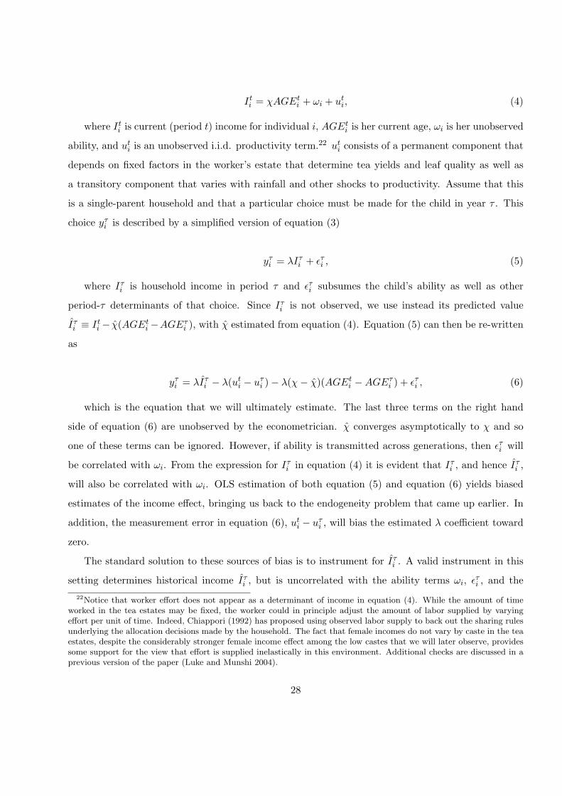
Iti = χAGEt
i + ωi + uti, (4)
where Iti is current (period t) income for individual i, AGEt
i is her current age, ωi is her unobserved
ability, and uti is an unobserved i.i.d. productivity term.22 ut
i consists of a permanent component that
depends on fixed factors in the worker’s estate that determine tea yields and leaf quality as well as
a transitory component that varies with rainfall and other shocks to productivity. Assume that this
is a single-parent household and that a particular choice must be made for the child in year τ . This
choice yτi is described by a simplified version of equation (3)
yτi = λIτ
i + ετi , (5)
where Iτi is household income in period τ and ετ
i subsumes the child’s ability as well as other
period-τ determinants of that choice. Since Iτi is not observed, we use instead its predicted value
Iτi ≡ It
i − χ(AGEti −AGEτ
i ), with χ estimated from equation (4). Equation (5) can then be re-written
as
yτi = λIτ
i − λ(uti − uτ
i ) − λ(χ − χ)(AGEti − AGEτ
i ) + ετi , (6)
which is the equation that we will ultimately estimate. The last three terms on the right hand
side of equation (6) are unobserved by the econometrician. χ converges asymptotically to χ and so
one of these terms can be ignored. However, if ability is transmitted across generations, then ετi will
be correlated with ωi. From the expression for Iτi in equation (4) it is evident that Iτ
i , and hence Iτi ,
will also be correlated with ωi. OLS estimation of both equation (5) and equation (6) yields biased
estimates of the income effect, bringing us back to the endogeneity problem that came up earlier. In
addition, the measurement error in equation (6), uti − uτ
i , will bias the estimated λ coefficient toward
zero.
The standard solution to these sources of bias is to instrument for Iτi . A valid instrument in this
setting determines historical income Iτi , but is uncorrelated with the ability terms ωi, ετ
i , and the22Notice that worker effort does not appear as a determinant of income in equation (4). While the amount of time
worked in the tea estates may be fixed, the worker could in principle adjust the amount of labor supplied by varyingeffort per unit of time. Indeed, Chiappori (1992) has proposed using observed labor supply to back out the sharing rulesunderlying the allocation decisions made by the household. The fact that female incomes do not vary by caste in the teaestates, despite the considerably stronger female income effect among the low castes that we will later observe, providessome support for the view that effort is supplied inelastically in this environment. Additional checks are discussed in aprevious version of the paper (Luke and Munshi 2004).
28
productivity shocks uti−uτ
i . Returning to the complete specification, with total household income and
female income as regressors, two instruments are required, satisfying the conditions described above.
To separately identify a total income (male plus female) and a female income effect, it is well known
that at least one of the statistical instruments that we choose must have a differential effect on male
and female income, and hence on total and female income.23
The first instrument that we propose takes advantage of the mountainous terrain and the enormous
variation in elevation - ranging from 1300 meters to 1900 meters - in the tea estates. Tea leaf yields
and quality vary substantially with elevation, and this (differentially) affects male and female incomes
across estates. Figure 2 presents nonparametric regressions of male and female income on estate
elevation. Male income increases monotonically in estate elevation, but this relationship is highly
nonlinear. Income increases steeply with elevation initially, then flattens out, before rising steeply once
again at higher elevations. Leaf quality improves at higher elevations, particularly above 5000 feet
(1600 meters), and higher quality teas require greater care and maintenance, which is the responsibility
of the male workers, so it is not surprising that male incomes are increasing with elevation in this
fashion. While the female income-elevation relationship is also highly nonlinear in Figure 2, the steady
increase in income with elevation that we saw for the men is absent. Female incomes depend on the
quantity of tea leaves plucked, rather than their quality, which explains why male and female incomes
respond differently to elevation.
Looking back at equation (6), estate elevation appears in the permanent component of the pro-
ductivity term and is thus uncorrelated with uti − uτ
i by construction. The identifying assumption
when using this instrument is that elevation is uncorrelated with (mean) ability among the workers in
the estate, and hence with their children’s ability. The historical patterns of migration described in
Section 2 suggest that workers were not sorted by ability across estates when their positions were first
made permanent in the 1930s. However, they could have subsequently circumvented the company’s
policy restricting movement across estates, if indeed the returns to ability varied with elevation, by
re-sorting through marriage. Selective exit from the High Range, once again through marriage, could
also have generated a link between elevation and the ability of the workers that remained. We describe
simple tests in the next section that demonstrate that re-sorting through marriage and selective exit
do not play an empirically significant role in this environment.23The empirical specification in equation (3) and the identification strategy that we propose below follows previous
empirical work on intra-household resource allocation. Notable contributions to this long and creative literature includeSchultz (1990), Thomas (1990), and more recently Duflo and Udry (2003).
29

Given the strong link between current income Iti and current age AGEt
i in Figure 1, and the
method that we use to adjust the income, the age at which parents make choices for their children
AGEτi clearly determines Iτ
i . It thus appears natural to construct an instrument based on those
sources of exogenous variation in AGEτi that are plausibly uncorrelated with the ability terms ωi, ετ
i ,
and the productivity shocks uti − uτ
i in equation (6).24
Children are sent to secondary school at a fixed age (10) and enter the marriage market at a fixed
age (assumed to be 16) in this economy. The age at which the single parent makes choices for her
child in equation (6) can then be expressed as
AGEτi = θ + AGECBi
where θ is the child’s age when choice yτi is made, which varies by the type of choice but is common
across households, and AGECBi is the parent’s age at childbirth. All of the variation in AGEτi comes
from the age at childbirth AGECBi, and we will use those components of AGECBi that are plausibly
uncorrelated with the unobserved determinants of yτi to construct an instrument for Iτ
i .
Allowing now for multiple children within the household, the age at childbirth for the j’th child in
household i can be described by the following expression:
AGECBij = MAGEi + pijNiSi + νij (7)
where MAGEi is the age at which the parent married, Ni is the number of children in the household
(parity), Si is the average spacing between births, pij = j/Ni measures the (normalized) birth order
of the child, and νij =∑j
k=1(Sik − Si) is the idiosyncratic deviation from the average birth spacing
in that household summed over all children born prior to child j. The discussion that follows will
study each component of AGECBij in equation (7), assessing whether it is uncorrelated with the
unobserved determinants of schooling and marriage choices in equation (3).
The first component of the age at childbirth AGECBij that we discuss is the marriage age MAGEi.
While the individual might enter the marriage market at a fixed age in this society, a standard two-
sided search model would predict that the age at marriage would in general depend on the individual’s24The separability between age and ability in equation (4) is commonly assumed but not innocuous. It is easy to
verify that terms containing AGEτi enter the residual of equation (6) if this assumption fails. Similarly, if credit markets
function smoothly and choices are based on lifetime income, then the age adjustment is unnecessary and AGEτi will
enter the residual of equation (6) once again. Tests of the overidentifying restrictions reported later will, however, allowus to verify the validity of this instrument.
30
ability (see, for instance, Luke and Munshi 2003). The parent’s age at marriage would be correlated
with the child’s unobserved ability in that case, to the extent that parental ability is transmitted
across generations. The instrument that we construct will consequently replace MAGEi in equation
(7) with the sample average MAGE.25
Next, consider fertility, measured by the number of children Ni and the average birth spacing Si.
While the unobserved term in equation (3) εij was previously interpreted as measuring the child’s
(unobserved) ability alone, this term could include the parents’ preferences for schooling and marriage
as well. Fertility is a choice made by the parents, and it is conceivable that this choice is jointly
determined with the schooling and marriage decisions by unobserved parental preferences.
A standard solution to this endogeneity problem would be to replace household fertility with
an aggregate fertility measure that is uncorrelated with idiosyncratic parental preferences. Fertility
declined rapidly in Kerala in the 1970s, with a fall in the total fertility rate from 4.0 in 1971-73 to
2.9 in 1979-81 (Sekher, Raju and Sivakumar 2001). Figure 3 presents nonparametric estimates of
the number of children ever born and the average birth spacing for the women in the sample. There
is a sharp decline in the number of children, from 4.8 to 3.5 for women currently between the ages
of 50 and 57, which coincides with the rapid state-wide fertility decline just described. The number
of children continues to decline thereafter, but at a slower rate, and some of the decline among the
younger women (less than 40) is no doubt because they have yet to reach their desired family size.
Higher-order births are associated with longer intervals, particularly when fertility is unrestricted, and
not surprisingly birth spacing declines (albeit relatively slowly) over the full 25-57 age range.26
We thus replace the household level statistics Ni, Si with their corresponding cohort averages Nc,
Sc to construct the age instrument
AGECBij = MAGE + pijNcSc + νij . (8)
Although the workers in the tea estates are Tamil, their fertility follows the general trend in Kerala
where they live; indeed, fertility in the low and high castes tracks very closely across all cohorts (not25It is evident from equation (7) that the only source of variation in the age at childbirth across parents within a
household is the age at marriage. Once MAGEi is replaced by MAGE it follows immediately that only a single ageinstrument is available even in a two-parent household.
26Prior to the fertility transition and deliberate fertility control, higher-order births occur at longer intervals as aconsequence of the decline in fecundity with mother’s age (Menken 1985). If the fertility transition is characterized bystopping behavior, in which higher-order (longer interval) births are prevented, then the decline in the number of childrenwill be associated with a shorter average birth interval (Knodel 1977).
31

reported) despite the differences in preferences for schooling and marriage documented above. The
decline in fertility below age 40 also follows in part from the truncation in family size at younger ages.
The mechanical increase in the age at childbirth with birth order pij and the idiosyncratic shocks to
birth spacing νij , which are for the most part biological, are treated as exogenous in the construction
of the instrument as well.27 It follows immediately from Figure 1 that the age instrument will have a
differential effect on male and female income, satisfying the second requirement for a valid instrument
in this setting.
It has been argued that gender and birth order affect the resources that the child receives in South
India (Behrman 1997, Pande 2003), and all of the regressions will include a boy dummy. The fact
that birth order affects household choices is not by itself a cause for concern as long as this variation
across siblings is driven by changes in available resources at the level of the household as the parents
get older. The concern here is that allocation across siblings might reflect a parental preference for
older (or younger) children. The first boy has a special position in the Indian household, since the
parents traditionally lived with him in old age. Recognizing that this additional responsibility could
affect choices that are made for him, the robust regressions that we report will include a first-boy
dummy as an additional regressor. Apart from the first boy we are aware of no societal preference
for particular children. The number of children could also directly determine household choices by
changing the resources available per child. Since Nc, Sc enter as interaction terms in equation (8)
above, the robust regressions that we report later will include the number of children in the household
Ni as an independent regressor.
The adjusted age instrument exploits two sources of variation in the age at child birth: changes in
fertility across cohorts of women and changes in birth order within the family. One concern with this
instrument is that preferences for schooling or ties to the network could vary independently across
cohorts of women, generating a spurious correlation between the instrument that we construct and
unobserved parental preferences across cohorts. A second concern is that the marriage and schooling
choices that parents make for their children could depend directly on the birth order.
To provide additional support for the validity of the adjusted age instrument we take advantage27The implicit assumption here is that birth spacing is independent of birth order, allowing us to treat νij as noise
within the household. Tests not reported with household fixed effects reveal that birth spacing is indeed uncorrelatedwith birth order except for the first birth interval, which is of shorter duration. We verified that including first-boy andfirst-girl dummies as additional regressors had no effect on the estimated income effects. Economic shocks could alsoaffect birth spacing, but we would not expect transitory shocks prior to the child’s birth to have a significant effect onthe schooling and marriage choices that are made for that particular child many years in the future.
32

of the fact that there are two independent sources of variation in this instrument: aggregate fertility
across cohorts and (normalized) birth order within the family. The instrumental variable regressions
can in principle be estimated by using a single source of variation in the adjusted age, purging the
constructed instrument of variation in the other source. The results, with each independent source
of variation alone, were reported in a previous version of the paper (Luke and Munshi 2004) and are
similar to what we will obtain with both sources of variation below. Our results do not appear to be
driven by a single source of variation in the adjusted age instrument, which implies in turn that either
of these independent sources of variation (with their associated concerns) cannot spuriously generate
the results that we obtain.
4.3 Regression Results
We begin the description of the regression results by presenting the first-stage regressions in Table
5. Recall that male income was initially increasing in estate elevation, then flattened out, before
increasing again at higher elevations in Figure 2. While the relationship between female income and
elevation was also non-linear, the initial increase observed for the men was absent. To allow for such
non-linearity in the income-elevation relationship we will include linear, quadratic, and cubic elevation
terms as instruments in all the regressions. Similarly, recall that female income was increasing steeply
with age until age 38 after which it continued to grow more slowly, whereas incomes declined at older
ages for the men. To account for these nonlinearities, linear and quadratic age terms will be included
as instruments. We discussed the importance of including parental education and whether the parents
were first-generation arrivals in the estates as controls in the second-stage regressions in Section 4.2,
and so these variables must be included in the first-stage regressions as well. A full set of jati dummies
is also included in both the first-stage and the second-stage regressions to estimate the income effects
within each jati, as required by the model laid out in Section 3.
Table 5, Columns 1-4 study the effect of elevation and age on current income, measured as the
average over the 1999-2001 period, separately by caste category. The linear, quadratic, and cubic
elevation coefficients are positive, negative, and then positive again, matching the patterns in Figure
2. The linear and quadratic age terms are positive and negative respectively, for men and women,
matching the patterns in Figure 1. All of the coefficients are very precisely estimated, and the pattern
of coefficients is qualitatively similar for the high castes and the low castes.28 Each of the instruments28The elevation-age interaction term has no effect on male or female income. Elevation can be interpreted as a measure
33

also has a differential effect on female income and total income, which we noted earlier is necessary
to separately identify the income effects. Although not reported, the parental characteristics that we
include as controls generally play an insignificant role in the income regressions.
Table 5, Columns 5-8 repeat the first-stage regression with income and age adjusted to the time
when the child was born. In addition, the adjusted female age is purged of variation in the marriage
age as well as variation in fertility within cohorts, as in equation (8). Without variation in the marriage
age, the husband’s adjusted age provides no additional information beyond what is contained in the
wife’s adjusted age and so no longer appears as an instrument. The unit of observation changes
from the household in Columns 1-4 to the individual child in Columns 5-8.29 The basic pattern of
coefficients reported earlier continues to be obtained. The nonlinearities in the elevation and age effects
are unchanged, the estimated coefficients continue to be precisely estimated, and the instruments have
a differential effect on female income and total income. The F-statistic testing the joint significance
of the excluded instruments is extremely large in all the first-stage regressions (the p-values are less
than 0.0001 without exception), indicating that there is sufficient power in the instruments that we
have chosen. We will later adjust incomes and ages to the time when the child was 10 years old
and 16 years old in the schooling, marriage, and residence regressions; the F-statistics continue to be
extremely large and the same patterns are obtained with those reduced samples of children, except
that the elevation coefficients are less precisely estimated.
Table 6 reports the second-stage schooling, marriage, and residence regressions. Recall that the
set of dependent variables includes a binary variable indicating whether the child married a relative,
a binary variable indicating whether the child was sent to school in the origin location, the child’s
educational attainment, and a binary variable indicating whether the child resides in the origin location
(conditional on having left home).30 The sample is restricted to children aged 10-40 with school
of estate-level ability. This useful result consequently provides some support for the assumption that ability enters asan additively separable term in the income equation (4). This result also suggests that the returns to ability do notvary with estate elevation, at least among the female workers, since their ability was previously seen to increase withexperience and hence age in Figure 1. When the returns to ability do not vary with elevation there is no incentive forworkers to sort across estates by ability, ruling out one channel through which the identifying assumption underlying theelevation instrument could be violated.
29The sample is restricted to children less than 41 years old in Columns 5-8. We include the child’s cohort (41 minuscurrent age) and sex in these regressions to match the second-stage regressions reported later.
30The marriage and residence regressions are estimated with a selected sample and it is easy to verify that theinstruments will no longer be valid if they determine the probability that the child is married or is no longer residingwith the parents. Conditional on the child’s age and sex, and the parental controls, the instruments have no effecton these probabilities. The analysis also omits those households in which the husband works outside the tea estates.Distance to Munnar determines whether the husband will work outside the estate but does not directly influence thelong-term choices that are made for the children, and so the predicted outcome (propensity score) from a job location
34
location as the dependent variable and children aged 16-40 with marriage, educational attainment,
and residential location as the dependent variables. Parental ages and incomes are consequently
adjusted to the time when the child was 10 years old in the school location regressions and 16 years
old in the remaining regressions.31
The second-stage regression was specified in equation (3) and includes as regressors (age-adjusted)
female and total income, the child’s cohort (41 minus current age), a boy dummy, parents’ schooling,
and whether the parents are first-generation arrivals in the tea estates. In addition, all regressions
include a full set of jati dummies.32 These controls are not reported in Table 6 to preserve space
but it is worth mentioning that schooling has increased rapidly over time and that parents’ schooling
has a large and statistically significant effect on children’s schooling, consistent with the results from
previous studies (see, for instance, Munshi and Rosenzweig 2003).
The second-stage regression analysis is implemented in four stages. The regressions reported in
Table 6, Panel A use estate elevation, father’s adjusted age, and mother’s adjusted age, together with
the appropriate higher-order terms for each variable, as instruments. We have already discussed the
potential problems with the adjusted age instrument, including the likely correlation between the age
at marriage and individual ability. Nonparametric regressions reported in a previous version of the
paper (Luke and Munshi 2004) revealed that the marriage age for the fathers had increased sharply in
recent years, suggesting that ability might have changed across cohorts. We consequently proceed to
replace marriage age for the fathers MAGEi with the sample marriage age MAGE. Once we purge the
regression that includes distance in addition to all the other terms in the first stage regression was included in theschooling, marriage, and residence second stage regressions to correct for selective employment outside the tea estates.Distance from Munnar has a positive and significant effect on the probability that the husband will remain inside theestates for both castes, as expected. However, inclusion of the propensity score has no effect on the income coefficientsin the second stage regressions for either caste, perhaps because the returns to ability are comparable inside and outsidethe estates.
31The regression that we use to adjust male and female current income has the same specification as the first-stageregression in Table 5, Columns 1-4, except that elevation is replaced by a full set of estate dummies to increase therobustness of the estimates. By assigning zero current income to unemployed men, and using the estimated age coefficientsto project back into the past, we are clearly underestimating incomes when those men were employed. The level ofunemployment increases very steeply after age 50 and so we verified that all the results go through with a reducedsample of households in which the husband was currently less than 50 years. We also considered alternative age rangesand age adjustments without changing any of the results. For the age adjustments we shifted the age three years beforeand three years after the age that we use in this paper (7 and 13 years and 13 and 19 years) and also experimented withthe seven-year average of the adjusted income (7-13 years and 13-19 years).
32With jati fixed effects we are effectively studying the effect of income variation within jatis, some of which arequite small. We consequently experimented with an alternative specification that omitted the jati fixed effects, withoutaffecting the results. Along the same lines, while there are only two low caste jatis, there are over 50 high caste jatis.We experimented with alternative samples that excluded jatis with less than 30 households in the sample, once againwithout changing any of the results.
35

instrument of variation in the marriage age, the father’s adjusted age provides no information beyond
what is contained in the mother’s age. The instruments in Panel B are consequently restricted to estate
elevation and the mother’s adjusted age, together with the higher-order terms associated with these
variables. Subsequently we report regressions in Panel C with the woman’s adjusted age constructed
as in equation (8), which implies that we are identified off variation in elevation, aggregate changes
in fertility across cohorts, mechanical variation in birth order within the household, and idiosyncratic
variation in birth spacing across children within the household. Finally, the number of children within
the household and the first-boy indicator are included as additional controls in Panel D.33
With two endogenous variables, female income and total household income, and the multiple
instruments that are available, we have many degrees of freedom. We expect to perform better on
the test of the overidentifying restrictions as the adjusted-age instrument is gradually purged of those
sources of variation that could directly determine schooling and marriage choices as above. The test
that we implement regresses the residual from any given regression on the full set of instruments used
in that regression and we report the F-statistic that tests the hypothesis that all the coefficients in
these regressions are zero in Table 6. While the marriage and residential location regressions pass
the test of the overidentifying restrictions comfortably in Panel A, the schooling regressions do not
(the p-values are less than 0.10). The tests reported in Panel B perform better; only the educational
attainment regression continues to fail. And, finally, all the robust regressions reported in Panel C
and Panel D comfortably pass the tests of the overidentifying restrictions as expected.
The theoretical framework laid out in Section 3 shows that an increase in household income could
lead to a decline in schooling if wealthier households were tied more closely to their networks. The
total income coefficient in the educational attainment regression is negative, particularly in Panel C
and Panel D. As predicted, the estimates in Table 6 indicate that an increase in household income
increases the probability that a child will marry a relative, attend secondary school in the origin
location, and ultimately settle there, for both castes without exception.
Conditional on household income, what effect does an increase in female income have on marriage
and schooling choices and residential outcomes? We argued in Section 3 that women, particularly
low caste women, might want to distance themselves and their families from the extended family33The survey collected individual-specific information on surviving children only. Ni is consequently measured as
the total number of surviving children rather than the number of children ever born in the regression analysis. Thisdiscrepancy is unlikely to affect our results since health services are readily available in the tea estates and so infant andchild mortality are quite low (company health statistics indicate that infant mortality in the tea estates, for example,was 18.8 per 1000 in 1999-2000).
36

network. Consistent with this view, a relative increase in female income lowers the probability that
the children will marry a relative or be schooled in the origin location, increases children’s schooling,
and consequently lowers the probability that the children will settle in the origin location in Table
6.34 While the female income effects go in the same direction for both castes, they are statistically
significant for the low castes alone. The point estimates are also substantially larger for the low
castes.35
The model laid out in Section 3 does not permit us to predict how the total income coefficient will
vary by caste. In general, no pattern is immediately discernable in Table 6, although the total income
effects are comparable for the two castes in a number of specifications. It is only the female income
coefficient that is substantially larger (in absolute magnitude) and more precisely estimated for the
low castes. To get a sense of the magnitude of the female income effects, households in the tea estates
earn Rs. 40,000 per year on average, with a Rs. 3,000 gap between the women and the men. Based on
the difference in the low caste and high caste female income coefficients in the schooling regression in
Panel D, this implies that over 50% of the caste-gap in schooling in Table 4 would be closed if incomes
were equalized within these households.
We argued in Section 3 that the low caste mothers might have a particularly strong incentive to
distance their daughters from the extended family network. To empirically investigate this prediction,
we proceed to estimate the income effects separately by caste and gender in Table 7, using the same
specification as in Table 6, Panel D. The results can be summarized as follows: First, the female
income effect continues to be larger in absolute magnitude and is more precisely estimated for the
low castes, both for boys and girls.36 Second, the low caste female income effect is much larger in
absolute magnitude for the girls than the boys with educational attainment and residential location as
the dependent variables. The low caste female income effect does not vary substantially with gender
for the remaining two outcomes. In contrast, the high caste female income effect, which is generally34When a child married a relative, the spouse is more likely to have grown up in the origin location, tying the child and
the family more closely to the home community. Although not reported, an increase in household income significantlyincreases the probability that the child’s spouse will have grown up in the origin location for both castes. Conditionalon household income, an increase in female income lowers the probability that the spouse grew up in the origin location.
35The point estimates are comparable for the two castes with marriage to a relative and secondary school locationas the dependent variables in Panel C and Panel D. These regressions, however, pass the test of the overidentifyingrestrictions comfortably in Panel A and Panel B and we note that the low caste female income effect is much larger thanthe corresponding effect for the high castes with those specifications.
36The point estimates for low castes and high castes are roughly comparable with marriage to a relative and secondaryschool location as the dependent variables, just as we saw in Table 6, Panel D. In a previous version of the paper (Lukeand Munshi 2004) we reported gender-specific estimates corresponding to the specification in Table 6, Panel A in whichthe low caste female income effects were substantially larger for both girls and boys.
37

insignificant, is of comparable magnitude for boys and girls with all the outcomes. The pattern of
female income effects by caste and gender thus appears to explain, in part, the striking observation
that low caste boys and girls had comparable levels of schooling in Table 4.37
4.4 Additional Results
The analysis in this paper is predicated on two important assumptions: First, that household decisions
in the tea estates are shaped by extended family networks in rural Tamil Nadu. And, second, that
the gender preference-gap is wider among the low castes than the high castes. The discussion that
follows provides independent support for each of these assumptions.
The idea that low caste households, particularly the women within these households, will want
to distance themselves from their inferior home networks seems plausible in this economic environ-
ment. However, other explanations for the caste differences that we observe are available. For example,
converts were drawn primarily from three low-caste jatis, Shanars, Paraiyars, and Pallars, when Chris-
tian missionaries arrived in Tamil Nadu at the beginning of the nineteenth century (Kent 2004). Not
surprisingly, 18% of low caste men and women versus 7% of high caste men and women in our sam-
ple report that they are Christian (these statistics are significantly different at the 5 percent level).
The Christian missionaries opposed traditional Hindu social practices, including marriage with close
relatives, while actively promoting education (Kooiman 1989). Thus, religious affiliation could, in
principle, explain the cross-caste patterns that we see in the data. Including the father’s and the
mother’s religious affiliation as regressors does not affect the results reported earlier, but there nev-
ertheless remains the possibility that some factor other than caste-networks that is common within
castes is driving the results.
Our response to this concern takes advantage of the fact that it is differences in networks, rather
than caste per se, that is seen to shape household choices in the tea estates. Just as caste provides
us with an exogenous measure of network quality, distance from the tea estates to the household’s
ancestral location will mechanically determine the strength of its ties to the network. While households
from distant communities might put more effort into maintaining ties with their networks, we expect
the first-order effect to dominate, with the strength of social ties being negatively correlated with
physical distance.37The disproportionate effect of female income on daughter’s schooling has been noted in previous studies (Duflo 2003,
Thomas 1990), but the results that we obtain are shown to depend importantly on the social group that the householdbelongs to.
38

Figure 4 nonparametrically tests this hypothesis by regressing the four outcomes in Table 6 and
Table 7 - marriage, school location, educational attainment, and residential location - on the distance
to the ancestral location.38 As expected, an increase in distance lowers the probability that the
child will be married to a relative, sent to school in the origin location, or ultimately settle there,
presumably because network ties are less strong. In contrast, educational attainment is steadily
increasing with distance, except for a downward dip beyond 500 km., consistent once again with the
view that community-based networks far away are influencing important household decisions in the
tea estates.
To test the statistical significance of the distance effects just described, we present parametric
regression estimates with the same outcomes in Table 8. Both low caste and high caste children
were pooled together in Figure 4 and one concern is that the distance effects that we obtained were
driven by systematic differences in distance by caste. Results not reported reveal that the low castes
are disproportionately represented in the distant locations, which could have confounded the distance
effects that we derived. To control for such confounding effects, a full set of jati dummies is included in
Table 8. A full set of estate dummies as well as the usual individual characteristics are also included in
these regressions. One remaining concern is that unobserved worker ability might vary with distance.
Reassuringly, we find no relationship between distance and one measure of ability - income - for both
male and female workers in Table 8, Columns 1-2.39
Table 8, Columns 3-6 report the relationship between distance and the four child outcomes con-
sidered in Figure 4, including the controls described above. Linear and quadratic distance terms are
included to allow for the non-linearities that were apparent in the Figure. All the distance coefficients
have the expected sign and are jointly significant at the 5 percent level for each outcome, verifying
the importance of the distance effect and, by extension, the role of the home networks in shaping
household decisions in the tea estates.38Detailed maps of Kerala and Tamil Nadu were scanned and geocoded to compute the distance by road (adjusting
for the hilly terrain) from Munnar, the main town in the tea estates, to each location in rural Tamil Nadu.39The empirical results reported in Table 6 indicate that children are more likely to be married into the network
as household income rises. Marriage patterns determine exit from the tea estates and so elevation, which determinesincome, would have been associated with levels of exit from the tea estates over multiple generations. This is not aproblem as long as those who exit are not selected by ability, but if the ability distribution among the workers thatremain depends on the level of exit, then elevation will no longer be a valid instrument. One simple test to rule out suchselective exit takes advantage of the fact that while both distance and elevation determine marriage patterns and, hence,the level of exit, distance should not directly determine income in the tea estates unless exit is selective. The absence ofa relationship between income and distance in our data suggests that the distribution of ability among the workers thatremains is independent of the level of exit (and entry).
39

Next, we proceed to verify the second major assumption of the paper, that the gender preference-
gap varies by caste. The standard assumption in the household bargaining literature (and its many
variants) is that a change in bargaining power within the household shifts resource allocation smoothly
along the Pareto frontier. In a society in which men have traditionally made all the important decisions
it is difficult to imagine that such shifts will take place without conflict, especially in the tea estates
where the women actually earn more than the men. If preferences differ by gender among the low
castes, and low caste women use their income to influence household decision-making, then we expect
the shifts in resources that follow to be accompanied by conflict, possibly escalating to marital violence.
If the absence of a female income effect among the high castes arises because preferences are aligned
within these households, then a relative increase in female income should have no effect on marital
violence.
The respondents in the survey were asked whether they had been beaten by their husbands in the
last year as well as over their lifetimes. Marital violence is widespread in the tea estates and 35%
of the low caste women versus 31% of the high caste women reported that they had been beaten in
the last year (the difference between castes is significant at the 5 percent level).The discussion above
suggests that at least some of this difference may be explained by conflict over resource allocation
within the low caste households.
Studies of marital violence typically include male characteristics such as age, education, employ-
ment status, and alcohol consumption, together with household characteristics, particularly income or
wealth, as regressors (Martin, Tsui, Maitra and Marinshaw 1999, Hoffman, Demo and Edwards 1994).
Those studies that are interested in disagreements over resource allocation include female income, or
other measures of female resources, as well (Rao 1997). The basic specification of the marital violence
regression that we estimate consequently includes the husband’s age, education, and whether he is a
first-generation arrival in the tea estates as regressors. Since there can be a social aspect to marital
violence, a full set of jati dummies is also included in these regressions. Finally, current total income
and current female income are included as regressors, which we instrument for with elevation (linear,
quadratic, and cubic terms) and the woman’s current age (linear and quadratic terms). Conflict today
will be determined by current and past household decisions and, hence, by current and past incomes.
We make the assumption as elsewhere in the paper that current conflict will depend disproportion-
ately on current incomes. This also implies that we no longer need to adjust incomes and the age
instruments as we did previously.
40
The assumptions that we must make to support the validity of the elevation instruments are
unchanged in the violence regressions. However, the woman’s age is no longer adjusted and so the
identifying assumption will change; conditional on the man’s age, which is included as a regressor,
the woman’s age must not directly determine marital violence. This equivalently implies that the age
difference between the husband and the wife must not determine marital violence. This condition
will be satisfied under the standard assumption that it is the resources that the husband and the
wife bring to the bargaining table, rather than their underlying characteristics, that determine the
allocation of resources within the household and hence the potential for conflict. However, we might
imagine that the woman’s ability to avoid potentially violent situations will improve with age and
experience. The age difference between the husband and the wife might also determine the respect
that he is accorded within the household, with implications for the incidence of marital violence.
Rejection of the identifying assumption for the age instrument will, however, lead to the failure of the
overidentifying restrictions, which we proceed to test below.
Table 9, Columns 1-2 report regression estimates with marital conflict in the last year (measured
as a binary variable) as the dependent variable. An increase in total household income reduces the
probability of marital violence among the low castes, perhaps because disagreements over resource
allocation are less likely to escalate into violence when overall economic conditions are favorable.
Conditional on total household income, an increase in female income increases the probability of
marital violence among the low castes, which is precisely what we would expect when there are
disagreements over resource allocation within the household. The husband’s age coefficient is also
negative and significant for the low castes, presumably because the choices that the household must
make, and the conflict that goes with them, will vary over the life-cycle. Although not reported, the
husband’s education and whether he is a first-generation arrival in the tea estates have no effect on
marital violence.
In contrast with the strong effects that we obtain for the low castes in Column 1, we see in Column
2 that total income, female income, and the husband’s age have no effect on marital violence among
the high castes. When there is no disagreement over resource allocation within the household, there
is no potential for violence at any level of household income or, for that matter, at any point in the
life-cycle (age). By the same reasoning, a relative increase in female income should have no effect on
marital violence.
The results in Columns 1-2 are consistent with the assumption that a gender preference-gap exists
41

among the low castes but not the high castes. The instruments that we use also comfortably pass the
tests of the overidentifying restrictions. Nevertheless, there remains the possibility that insignificant
coefficients for the high castes in Column 2 are obtained simply because the self-reported incidence
of marital violence by the survey respondents is a noisy measure of the true incidence. The survey
collected information not only on the incidence of marital violence but also on the frequency of violence
in the past year. Table 8, Columns 3-4 uses repeated marital violence (two or more times) in the past
year, which is probably more precisely measured as the dependent variable, yet obtains essentially
the same results.40 As a final check we include a binary variable indicating whether the husband
drinks regularly as an additional regressor in Table 8, Columns 5-6. The idea here is to see whether
the association between violence and alcohol consumption, which has been found in many previous
studies (as in, for instance, Rao 1997), is similar for low castes and high castes. While the coefficient
on the alcohol variable is difficult to interpret, it is very precisely estimated and close in magnitude
for the two castes. The income coefficients in Columns 5-6 remain very similar to what we obtained
in Columns 1-4; it is only with the income effects, which are associated with conflict over resource
allocation within the household, that large caste differences are consistently obtained.
5 Conclusion
Disparities in income and education persist across social groups in many developing countries such
as India even as globalization proceeds around the world. This paper explores the role that women
might play in reducing these disparities. We argue that low caste women, who have historically been
disadvantaged in terms of both caste and gender, might have a disproportionately strong incentive to
distance themselves and their families from the tradition network-based economy and invest instead
in their children’s human capital when resources are made available to them.
Female workers earn substantially more than male workers on the tea estates, and these unusual
gender patterns have been in place for multiple generations. Controlling for total household income,
we find that an exogenous increase in female income among the low castes increases investments in
schooling and lowers the probability that the children will marry into the network in the traditional
fashion, be sent to school in the family’s ancestral location, or ultimately end up living there. In
contrast, a relative increase in female income has no effect on household decisions among the high40The incidence of marital violence drops substantially with this measure to 20% for the low castes versus 17% for the
high castes. The difference between the castes is close to significant at conventional levels (p=0.07).
42
castes. This difference in the female income effect can explain, in part, the striking observation that
educational attainment is higher among the low castes than the high castes in the tea estates. Low
castes and high castes have the same income and access to the same facilities on the tea estates. The
low castes appear to invest at least as much as the high castes in their children’s human capital, once
the usual cross-caste disparities in income and access are controlled for.
43

References
[1] Akresh, Richard. 2004. Risk, Network Quality, and Family Structure: Child Fostering Decisions
in Burkina Faso, BREAD Working Paper No. 065.
[2] Alexander, K.C. 1989. Caste Mobilization and Class Consciousness: The Emergence of Agrarian
Movements in Kerala and Tamil Nadu, in: F.R. Frankel and M.S.A. Rao (eds), Dominance and
State Power in Modern India; Decline of a Social Order, vol.1, Delhi: Oxford University Press,
p. 362-413.
[3] Baak, Paul Erik. 1997. Plantation, Production and Political Power: Plantation Development in
South West India 1743-1963. Delhi: Oxford University Press.
[4] Behrman, Jere R. 1997. Intrahousehold Distribution and the Family, in: Mark R. Rosenzweig
and Oded Stark (eds), Handbook of Population and Family Economics, Amsterdam: Elsevier, p.
125-187.
[5] Browning, Martin, Franois Bourguignon, Pierre-Andr Chiappori, and Valrie Lechene. 1994. In-
come and Outcomes: A Structural Model of Intrahousehold Allocation, Journal of Political Econ-
omy 102(6):1067-1096.
[6] Chakravarti, Uma. 1993. Conceptualizing Brahmanical Patriarchy in Early India: Gender, Caste,
Class and State, Economic and Political Weekly, 3 April.
[7] Chiappori, Pierre-Andr. 1992. Collective Labor Supply and Welfare, Journal of Political Economy
100(31):437-467.
[8] Cox, Donald. 2003. Private Transfers within the Family: Mothers, Fathers, Sons and Daughters,
in: Alicia H. Munnell and Annika Sunden (eds), Death and Dollars: The Role of Gifts and
Bequests in America, Washington D.C.: The Brookings Institution Press, p. 168-216.
[9] Duflo, Esther. 2003. Grandmothers and Granddaughters: Old Age Pension and Intra-household
Allocation in South Africa, World Bank Economic Review 17(1):1-25.
[10] Duflo, Esther and Christopher Udry. 2003. Intrahousehold Resource Allocation in Cote d’Ivoire:
Social Norms, Separate Accounts and Consumption Choices, BREAD Working Paper No. 016.
44
[11] Dumont, L. 1986. A South Indian Subcaste. Delhi: Oxford University Press.
[12] Geetha, V. 2002. Gender, Calcutta: Stree Publishers.
[13] Hardle, Wolfgang. 1990. Applied Nonparametric Regression, Econometric Society Monographs
No.11, Cambridge: Cambridge University Press.
[14] Hellerstein, Judith K. and David Neumark.. 1995. Are Earnings Profiles Steeper Than Productiv-
ity Profiles? Evidence from Israeli Firm-Level Data, The Journal of Human Resources 30(1):89-
112.
[15] Hjejle, Benedicte. 1967. Slavery and Agricultural Bondage in South India in the Nineteenth
Century, The Scandinavian Economic History Review XV(1,2):71-126.
[16] Hoffman, K.L., D.H. Demo, and J.N. Edwards. 1994. Physical wife abuse in a non-western society:
An integrated theoretical approach, Journal of Marriage and the Family, 56(1):131-146.
[17] Ilmakunnas, Pekka, Mika Maliranta, and jari Vainiomaki. 1999. The Roles of Employer and
Employee Characteristics for Plant Productivity, Helsinki School of Economics and Business
Administration Working Paper W-223.
[18] Kapadia, Karin. 1995. Siva and Her Sisters; Gender, Caste, and Class in Rural South India.
Boulder: Westview Press.
[19] Karve, Irawati. 1953. Kinship Organization in India. New York: Asia Publishing House.
[20] Kent, Eliza F. 2004. Converting Women; Gender and Protestant Christianity in Colonial South
India. Oxford: Oxford University Press.
[21] Knodel, John. 1977. Family Limitation and the Fertility Transition: Evidence from the Age
Patterns of Fertility in Europe and Asia, Population Studies 31(2):219-249.
[22] Kooiman, Dick. 1989. Conversion and Social Equality in India; the London Missionary Society
in South-Travancore in the 19th Century, Delhi: Manohar Press.
[23] Kumar, Dharma. 1965. Land and Caste in South India; Agricultural Labour in the Madras Pres-
idency During the Nineteenth Century, Cambridge: Cambridge University Press.
45
[24] Luke, Nancy and Kaivan Munshi. 2003. New Roles for Marriage in Urban Africa, MIT Department
of Economics Working Paper No. 03-20.
[25] Luke, Nancy and Kaivan Munshi. 2004. Women as Agents of Change: Female Incomes and
Household Decisions in South India, BREAD Working Paper No. 087.
[26] Lundberg, Shelly and Robert A. Pollak. 1993. Separate Spheres Bargaining and the Marriage
Market, Journal of Political Economy 101(6):988-1009.
[27] Manser, Marilyn and Murray Brown. 1980. Marriage and Household Decision Making: A Bar-
gaining Analysis, International Economic Review 21(1):31-44.
[28] Martin, S., A. Tsui, K. Maitra, and R. Marinshaw. 1999. Domestic Violence in Northern India,
American Journal of Epidemiology 150:417-426.
[29] McElroy, Marjorie B. and Mary Jean Horney. 1981. Nash Bargained Household Decisions, Inter-
national Economic Review 22(2):333-350.
[30] Menken, Jane. 1985. Age and Fertility: How Late Can You Wait?, Demography 22:469-484.
[31] Munshi, Kaivan and Mark Rosenzweig. 2003. Traditional Institutions Meet the Modern World:
Caste, Gender and Schooling Choice in a Globalizing Economy, BREAD Working Paper No. 038.
[32] Pande, Rohini P. 2003. Selective Gender Differences in Childhood Nutrition and Immunization
in Rural India: The Role of Siblings, Demography 40(3):395-418.
[33] Rao, Vijayendra. 1997. Wife-beating in Rural South India: A Qualitative and Econometric Anal-
ysis, Social Science and Medicine 44(8):1169-1180.
[34] Rubin, D. Kate and Jeffrey M. Perloff. 1993. Who Works for Piece Rates and Why, American
Journal of Agricultural Economics 75:1036-1043.
[35] Schultz, T. Paul. 1990. Testing the Neoclassical Model of Family Labor Supply and Fertility, The
Journal of Human Resources 25(4):599-634.
[36] Sekher, T.V., K.N.M. Raju and M.N. Sivakumar. 2001. Fertility Transition in Karnataka: Levels,
Trends and Implications, Economic and Political Weekly December 22: 4742-4752.
46

[37] Shearer, Bruce. 1996. Piece-Rates, Principal-Agent Models, and Productivity Profiles: Parametric
and Semi-Parametric Evidence from Payroll Records, The Journal of Human Resources 31(2):275-
303.
[38] Strauss, J. and D. Thomas. 1995. Human Resources: Empirical Modeling of Household and Family
Decisions, in: J. Behrman and T.N. Srinivasan (eds), Handbook of Development Economics,
Amsterdam: North Holland.
[39] Thomas, Duncan. 1990. Intra-household Resource Allocation: An Inferential Approach, The Jour-
nal of Human Resources 25(4):635-64.
[40] Trautmann, T.R. 1981. Dravidian Kinship. Cambridge: Cambridge University Press.
47

Table 1: Caste Comparisons in Tamil Nadu
Gender: men womenResidential location: rural urban rural urbanCaste: low high low high low high low high
(1) (2) (3) (4) (5) (6) (7) (8)Age 38.29 38.58 36.86 38.43 * 32.03 32.23 31.74 32.56
(0.41) (0.24) (0.49) (0.23) (0.33) (0.20) (0.42) (0.20)Schooling 4.23 5.61 * 7.18 8.79 * 3.39 3.39 3.46 3.66 *
(0.15) (0.10) (0.22) (0.11) (0.08) (0.04) (0.09) (0.04)Employed 0.98 0.99 0.97 0.98 0.76 0.57 * 0.39 0.32 *
(0.01) (0.003) (0.01) (0.003) (0.02) (0.00) (0.02) (0.01)Skilled job 0.23 0.39 * 0.60 0.80 * 0.06 0.13 * 0.13 0.22 *
(0.02) (0.01) (0.02) (0.01) (0.01) (0.01) (0.02) (0.01)
No. of observations 632 1,670 360 1,596 707 1,856 393 1,717
Note: standard errors in parentheses. * denotes rejection of the equality of means for the two caste groups at the 5 percent significance level.Low caste includes all Scheduled Castes as classified by the Government of India. High caste includes all other castes.Schooling is measured in years. Skilled job includes skilled labor and professional occupations.Data are from 1999 National Family Health Survey (NFHS) for Tamil Nadu.

Table 2: Caste Comparisons in Tea Estates
Gender: men women
Caste: low high low high(1) (2) (3) (4)
Panel A: Individual characteristics
Age 41.90 41.92 38.46 38.34(0.17) (0.26) (0.16) (0.24)
Income 18.58 19.02 21.46 21.43(0.19) (0.28) (0.09) (0.13)
Schooling 5.97 5.56 * 3.84 3.34 *(0.06) (0.09) (0.07) (0.09)
Panel B: Marriage and retirement
Married within jati -- -- 0.98 0.95 *(0.003) (0.01)
Married to relative -- -- 0.54 0.64 *(0.01) (0.01)
First generation worker 0.08 0.15 * 0.14 0.26 *(0.01) (0.01) (0.01) (0.01)
Parents retired in origin location 0.29 0.40 * 0.37 0.47 *(0.01) (0.02) (0.01) (0.02)
No. of observations 2,515 1,181 2,515 1,181
Note: standard errors in parentheses. * denotes rejection of the equality of means at the 5 percent significance level.Woman refers to the respondent and Man to her husband.Low castes include Pallars and Paraiyars. High castes includes all other jatis . Schooling is measured in years. Income is measured in thousands of Rupees per year.First generation workers are those that grew up outside the tea estates.Parents retired in origin location if they settled either in the father's or the mother's origin location in Tamil Nadu.

Table 3: Female Autonomy and Husband's Participation in Household Tasks
Subject: female workers mothers of female workersCaste: low high low high
(1) (2) (3) (4)
Panel A: Measures of female autonomy
Could buy sari or jewellery without permission 0.30 0.34 * 0.24 0.28 *(0.01) (0.01) (0.01) (0.01)
Could remit money to parents without permission 0.25 0.28 * 0.22 0.24(0.01) (0.01) (0.01) (0.01)
Collects her own salary (all workers) 0.14 0.19 * -- --(0.01) (0.01)
Collects her own salary (husband works on estate) 0.07 0.09 * -- --(0.01) (0.01)
Panel B: Husband helps with routine housework
Cooking 0.51 0.49 -- --(0.01) (0.01)
Washing 0.05 0.04 -- --(0.004) (0.006)
Childcare 0.39 0.37 -- --(0.01) (0.01)
No. of observations 2,509 1,178 2,403 1,116
Note: standard errors in parentheses. Low castes include Pallars and Paraiyars. High castes include all other jatis .Each autonomy question is coded as a binary variable, which takes the value one if the response is "yes" and zero if "no."The question whether the worker collects her own salary is coded separately for all workers and for those whose husbands work on the estates.Each housework question takes the value one if the husband helps "usually" or "sometimes" and zero if "rarely" or "never."
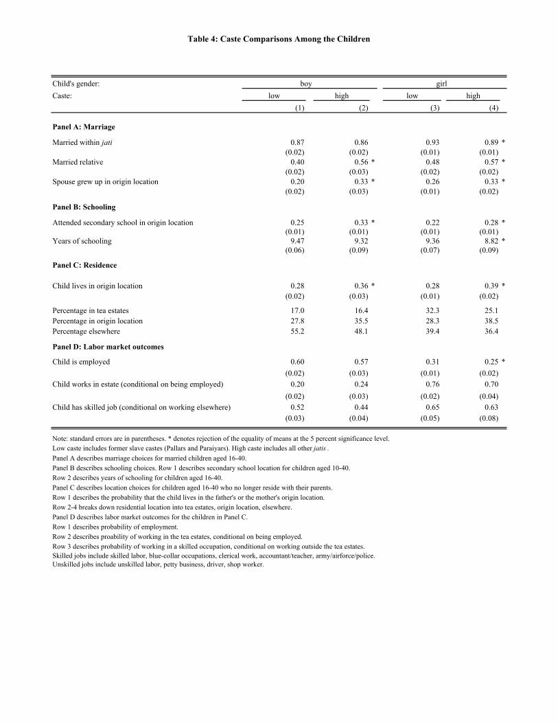
Table 4: Caste Comparisons Among the Children
Child's gender: boy girlCaste: low high low high
(1) (2) (3) (4)
Panel A: Marriage
Married within jati 0.87 0.86 0.93 0.89 *(0.02) (0.02) (0.01) (0.01)
Married relative 0.40 0.56 * 0.48 0.57 *(0.02) (0.03) (0.02) (0.02)
Spouse grew up in origin location 0.20 0.33 * 0.26 0.33 *(0.02) (0.03) (0.01) (0.02)
Panel B: Schooling
Attended secondary school in origin location 0.25 0.33 * 0.22 0.28 *(0.01) (0.01) (0.01) (0.01)
Years of schooling 9.47 9.32 9.36 8.82 *(0.06) (0.09) (0.07) (0.09)
Panel C: Residence
Child lives in origin location 0.28 0.36 * 0.28 0.39 *(0.02) (0.03) (0.01) (0.02)
Percentage in tea estates 17.0 16.4 32.3 25.1Percentage in origin location 27.8 35.5 28.3 38.5Percentage elsewhere 55.2 48.1 39.4 36.4
Panel D: Labor market outcomes
Child is employed 0.60 0.57 0.31 0.25 *(0.02) (0.03) (0.01) (0.02)
Child works in estate (conditional on being employed) 0.20 0.24 0.76 0.70(0.02) (0.03) (0.02) (0.04)
Child has skilled job (conditional on working elsewhere) 0.52 0.44 0.65 0.63(0.03) (0.04) (0.05) (0.08)
Note: standard errors are in parentheses. * denotes rejection of the equality of means at the 5 percent significance level.Low caste includes former slave castes (Pallars and Paraiyars). High caste includes all other jatis .Panel A describes marriage choices for married children aged 16-40. Panel B describes schooling choices. Row 1 describes secondary school location for children aged 10-40. Row 2 describes years of schooling for children aged 16-40. Panel C describes location choices for children aged 16-40 who no longer reside with their parents.Row 1 describes the probability that the child lives in the father's or the mother's origin location.Row 2-4 breaks down residential location into tea estates, origin location, elsewhere.Panel D describes labor market outcomes for the children in Panel C.Row 1 describes probability of employment.Row 2 describes proability of working in the tea estates, conditional on being employed.Row 3 describes probability of working in a skilled occupation, conditional on working outside the tea estates.Skilled jobs include skilled labor, blue-collar occupations, clerical work, accountant/teacher, army/airforce/police.Unskilled jobs include unskilled labor, petty business, driver, shop worker.

Table 5: First Stage Regressions
Income construction: current income age-adjusted incomeCaste: low high low highDependent variable: female inc. total inc. female inc. total inc. female inc. total inc. female inc. total inc.
(1) (2) (3) (4) (5) (6) (7) (8)
Elevation 47.041 122.879 28.845 109.458 35.609 94.022 16.460 105.271(16.998) (35.782) (15.391) (36.356) (16.903) (42.333) (17.964) (36.598)
Elevation-squared -3.016 -7.727 -2.007 -7.195 -2.285 -5.913 -1.214 -6.907(1.089) (2.276) (0.969) (2.303) (1.089) (2.727) (1.134) (2.319)
Elevation-cubed 0.064 0.161 0.046 0.157 0.048 0.123 0.029 0.150(0.023) (0.048) (0.020) (0.048) (0.023) (0.058) (0.024) (0.049)
Woman's age 1.141 0.822 1.322 1.826 1.076 1.536 1.065 1.128(0.152) (0.275) (0.174) (0.290) (0.217) (0.450) (0.308) (0.652)
Woman's age-squared -0.014 -0.008 -0.016 -0.021 -0.014 -0.016 -0.013 -0.008(0.002) (0.004) (0.002) (0.004) (0.005) (0.009) (0.006) (0.013)
Man's age 0.559 2.628 0.539 2.487 -- -- -- --(0.148) (0.278) (0.136) (0.300)
Man's age-squared -0.005 -0.033 -0.005 -0.031 -- -- -- --(0.002) (0.004) (0.002) (0.004)
R2 0.341 0.198 0.394 0.275 0.213 0.104 0.299 0.162F 76.21 43.75 89.26 121.20 96.96 62.62 83.85 55.09
Number of observations 2,240 2,240 1,049 1,049 5,903 5,903 2,793 2,793
Note: Standard errors in parentheses. Standard errors are robust to heteroscedasticity and clustered residuals within each estate.Low caste refers to former slave castes - Pallars and Paraiyars. High caste includes all other jatis . Elevation is measured in hundreds of meters. First generation workers are those who grew up outside the estates.Columns 1-4: each female worker is the unit of observation. Columns 5-8: each of her children currently aged 40 and under is the unit of observation.Woman's age, female income, household income are adjusted to the year in which the child was born in Columns 5-8.Adjusted woman's age is purged of variation in marriage age and variation in fertility within cohorts.All regressions include a full set of jati dummies and the man's and woman's years of schooling and whether they are first-generation workers.Columns 5-8 include child's cohort (41 minus current age) and gender as additional regressors.F statistic measures the joint significance of the excluded instruments.

Table 6: Marriage, Schooling and Residential Location
Dependent variable: child married relative secondary schol in origin years of schooling child resides in originCaste: low high low high low high low high
(1) (2) (3) (4) (5) (6) (7) (8)Panel A: First Set of Instruments
Female income -0.065 -0.013 -0.033 -0.020 0.213 0.058 -0.056 -0.034(0.025) (0.017) (0.011) (0.021) (0.104) (0.091) (0.019) (0.015)
Total income 0.022 0.007 0.009 0.032 0.003 -0.023 0.011 0.015(0.010) (0.006) (0.006) (0.012) (0.028) (0.030) (0.008) (0.006)
Overid test (F statistic) 0.49 0.59 7.09 5.04 3.64 2.58 0.89 0.28Overid test (p-value) 0.85 0.77 0.00 0.00 0.00 0.01 0.52 0.96
Panel B: Second Set of InstrumentsFemale income -0.056 -0.016 -0.135 -0.069 0.354 0.150 -0.082 -0.038
(0.028) (0.018) (0.045) (0.045) (0.156) (0.100) (0.036) (0.020)Total income 0.014 0.014 0.068 0.071 -0.105 -0.112 0.026 0.017
(0.014) (0.011) (0.025) (0.019) (0.077) (0.068) (0.018) (0.013)Overid test (F statistic) 0.49 0.37 0.68 0.64 2.78 1.31 0.28 0.20Overid test (p-value) 0.79 0.87 0.64 0.67 0.02 0.26 0.92 0.96
Panel C: Third Set of InstrumentsFemale income -0.045 -0.040 -0.101 -0.116 0.251 0.161 -0.067 -0.022
(0.025) (0.020) (0.033) (0.053) (0.143) (0.131) (0.033) (0.030)Total income 0.010 0.015 0.056 0.086 -0.120 -0.156 0.010 0.009
(0.011) (0.007) (0.018) (0.020) (0.060) (0.067) (0.016) (0.016)Overid test (F statistic) 0.44 0.30 1.12 0.22 1.81 0.38 0.75 0.17Overid test (p-value) 0.82 0.91 0.35 0.96 0.11 0.87 0.59 0.97
Panel D: Including number of children and first-boy indicator as controlsFemale income -0.055 -0.038 -0.092 -0.098 0.285 0.143 -0.065 -0.020
(0.026) (0.020) (0.032) (0.058) (0.144) (0.160) (0.032) (0.030)Total income 0.012 0.015 0.054 0.081 -0.135 -0.181 0.010 0.006
(0.013) (0.007) (0.017) (0.022) (0.061) (0.073) (0.016) (0.018)Overid test (F statistic) 0.54 0.29 1.17 0.48 1.27 0.12 0.77 0.06Overid test (p-value) 0.75 0.92 0.32 0.79 0.27 0.99 0.57 1.00Number of observations 1,235 651 4,346 2,069 3,302 1,585 1,707 819Note: Standard errors in parentheses. Standard errors are robust to heteroscedasticity and clustered residuals within each estate.Sample restricted to married children aged 16-40 in Columns 1-2, to children aged 10-40 in Columns 3-4, and to children aged 16-40 in Columns 5-8.Low caste restricted to former slave castes - Pallars and Paraiyars. Regressions include a full set of jati dummies, the parents' years of schooling and whether they are first-generation.Income is measured in thousands of Rupees per year. Cohort is computed as 46 minus current age.Incomes and ages are adjusted to the year in which the child was 16 years old in Columns 1-2 and Columns 5-8 and the year in which the child was 10 years old in Columns 3-4.First set of instruments includes elevation (linear, quadratic, cubic terms), and man and woman's adjusted age (linear and quadratic terms).Second and third set of instruments include elevation (linear, quadratic, cubic terms) and woman's adjusted age (linear and quadratic terms).The woman's adjusted age is purged of variation in marriage age across the full sample and variation in fertility across households in the same cohort in the third set of instruments.Panel D includes the number of children in the household and a first-boy indicator as controls.

Table 7: Marriage, Schooling, and Residential Location by Gender
Caste: low high low highChild's gender: girl boy girl boy girl boy girl boy
(1) (2) (3) (4) (5) (6) (7) (8)Panel A: Parental choices
Dependent variable: child married relative child attended secondary school in origin location
Female income -0.037 -0.072 -0.050 -0.063 -0.114 -0.085 -0.070 -0.100(0.034) (0.037) (0.035) (0.033) (0.053) (0.033) (0.055) (0.085)
Total income 0.001 0.021 0.032 -0.014 0.051 0.063 0.064 0.082(0.017) (0.009) (0.016) (0.014) (0.025) (0.015) (0.022) (0.034)
Overid test (F statistic) 0.32 0.12 0.87 0.31 0.58 0.29 0.45 0.52Overid test (p-value) 0.90 0.99 0.50 0.91 0.71 0.92 0.81 0.76
Number of observations 811 409 435 213 2,088 2,215 979 1,084
Panel B: Children's outcomes
Dependent variable: years of schooling child resides in origin locationFemale income 0.490 0.099 0.197 0.182 -0.071 -0.009 -0.028 -0.032
(0.269) (0.133) (0.183) (0.192) (0.043) (0.038) (0.036) (0.046)Total income -0.191 -0.037 -0.153 -0.219 0.012 -0.011 0.023 -0.004
(0.104) (0.069) (0.086) (0.072) (0.017) (0.018) (0.014) (0.025)Overid test (F statistic) 0.85 0.40 0.06 0.15 0.56 0.72 0.23 0.69Overid test (p-value) 0.52 0.85 1.00 0.98 0.73 0.61 0.95 0.63
Number of observations 1,576 1,699 757 821 978 712 491 324
Note: Standard errors in parentheses. Standard errors are robust to heteroscedasticity and clustered residuals within each estate.
Sample restricted to married children aged 16-40 in Panel A, Columns 1-4, to children aged 10-40 in Panel A, Columns 5-8, and to children aged 16-40 in Panel B.Low caste refers to former slave castes - Pallars and Paraiyars. High caste includes all other jatis .
Income is measured in thousands of Rupees per year. Cohort is computed as 46 minus current year.
All regressions include a full set of jati dummies and the man's and the woman's years of schooling and whether they are first-generation workers.
Incomes and ages are adjusted to the year in which the child was 16 years old in Panel A, Columns 1-4 and Panel B.Incomes and ages are adjusted to the year in which the child was 10 years old in Panel A, Columns 5-8.Instruments include elevation (linear, quadratic, cubic terms), and woman's adjusted age (linear and quadratic terms).The woman's adjusted age is purged of variation in marriage age across the full sample and variation in fertility across households in the same cohort.The number of children in the household and a first-boy indicator are included as controls.

Table 8: Household Decisions and Distance to Origin
Dependent variable: female income total incomechild married
relativesecondary school
in originyears of
schoolingchild resides
in origin(1) (2) (3) (4) (5) (6)
Distance to origin 0.079 -0.027 0.027 -0.067 0.041 -0.150(0.109) (0.539) (0.034) (0.027) (0.017) (0.028)
Distance to origin - squared -0.011 0.009 -0.006 0.003 -0.006 0.019(0.015) (0.060) (0.003) (0.003) (0.002) (0.003)
Joint sig. (F statistic) 0.26 0.25 4.87 22.08 3.10 22.35Joint sig. (p-value) 0.77 0.78 0.01 0.00 0.04 0.00
Number of observations 3,281 3,281 2,124 7,157 5,479 2,812
Note: Standard errors in parentheses. Standard errors are robust to heteroscedasticity and clustered residuals within each origin location.Origin refers to the female worker's origin location. Distance to origin is measured in hundreds of km.The household is the unit of observation in Columns 1-2 and the child is the unit of observation in Columns 3-6.Sample restricted to married children aged 16-40 in Column 3, to children aged 10-40 in Column 4, to children aged 16-40 in Column 5, and to children aged 16-40 who have left the parental home in Column 6.All regressions include a full set of jati and estate dummies.Columns 1-2 also include female worker's and male worker's age and age-squared.Columns 3-6 also include the child's age and gender.Joint sig. (F tstatistic) and Joint sig. (p-value) reports the F statistic and p-value for the test of the joint significance of the distance terms.

Table 9: Income and Marital Violence
Dependent variable: hit in the last year hit repeatedly in the last yearCaste: low high low high low high
(1) (2) (3) (4) (5) (6)
Female income 0.072 0.009 0.066 -0.0002 0.059 -0.017(0.037) (0.053) (0.030) (0.044) (0.037) (0.038)
Total income -0.035 -0.002 -0.033 0.003 -0.031 0.010(0.017) (0.024) (0.013) (0.020) (0.017) (0.016)
Husband's age -0.021 -0.006 -0.019 -0.001 -0.018 0.002(0.009) (0.012) (0.007) (0.009) (0.009) (0.008)
Husband drinks regularly -- -- -- -- 0.228 0.290(0.044) (0.038)
Overid test (F statistic) 0.21 0.72 0.07 0.87 0.23 0.50Overid test (p-value) 0.96 0.61 0.99 0.50 0.95 0.78
Number of observations 2,242 1,050 2,242 1,050 2,242 1,050
Note: Standard errors in parentheses. Standard errors are robust to heteroscedasticity and clustered residuals within each estate.Hit repeatedly if beaten two times or more in the last year.Low caste restricted to former slave castes - Pallars and Paraiyars. High caste includes all other jatis .Income is measured in thousands of Rupees per year. Regressions include a full set of jati dummies and husband's schooling and whether he is a first-generation worker.Instruments includes elevation (linear, quadratic, cubic terms), and woman's age (linear and quadratic terms).


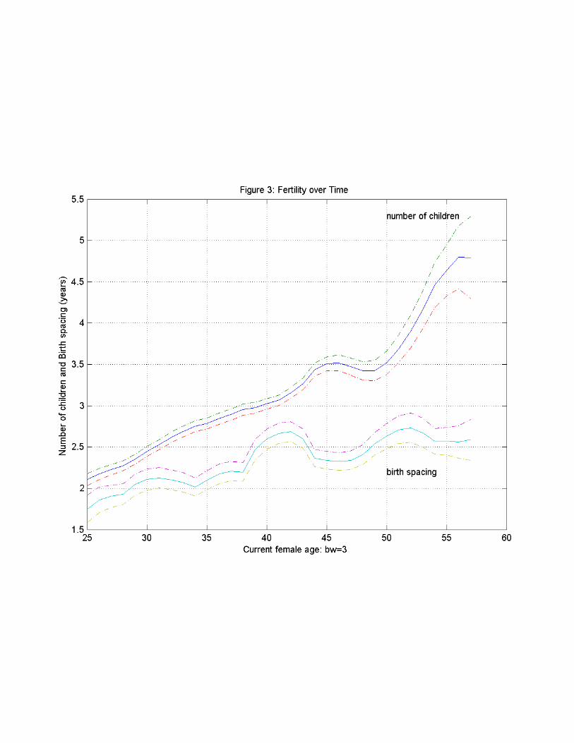


![[DPnF] Female x Female = Love](https://img.pdfslide.net/doc/110x75/577cd9a01a28ab9e78a3c67d/dpnf-female-x-female-love.jpg)